Detection of bursts in extracellular spike trains

using hidden semi-Markov point process models

Surya TokdarDepartment of Statistics

Carnegie Mellon University

Pittsburgh, PA 15213

Email: stokdar@stat.cmu.edu

Phone: (412) 268 3556

Fax: (412) 268 7828

Peiyi XiDepartment of Statistics

Carnegie Mellon University

Pittsburgh, PA 15213

Ryan C. KellyDepartment of Computer Science

Center for the Neural Basis of Cognition

Carnegie Mellon University

Pittsburgh, PA 15213

Robert E. KassDepartment of Statistics

Center for the Neural Basis of Cognition

Carnegie Mellon University

Pittsburgh, PA 15213

May 20, 2009

Abstract

Neurons in vitro and in vivo have epochs of bursting or “up state” ac-tivity during which firing rates are dramatically elevated. Various meth-ods of detecting bursts in extracellular spike trains have appeared inthe literature, the most widely used apparently being Poisson Surprise(PS). A natural description of the phenomenon assumes (1) there are twohidden states, which we label “burst” and “non-burst,” (2) the neuronevolves stochastically, switching at random between these two states, and(3) within each state the spike train follows a time-homogeneous pointprocess. If in (2) the transitions from non-burst to burst and burst tonon-burst states are memoryless, this becomes a hidden Markov model(HMM). For HMMs, the state transitions follow exponential distributions,

1

and are highly irregular. Because observed bursting may in some cases befairly regular—exhibiting inter-burst intervals with small variation—werelaxed this assumption. When more general probability distributions areused to describe the state transitions the two-state point process modelbecomes a hidden semi-Markov model (HSMM). We developed an effi-cient Bayesian computational scheme to fit HSMMs to spike train data.Numerical simulations indicate the method can perform well, sometimesyielding very different results than those based on PS.

Keywords: Hidden Markov Model, Markov-Modulated Poisson Process, Pois-son Switching Model, Poisson Surprise, Rank Surprise, Up State

2

1 Introduction

Extracellularly-recorded spike trains often contain clusters of several spikes, sep-arated by unusually small inter-spike intervals (ISIs). Such clusters may repre-sent sudden epochs of elevated firing rate due to a neuron’s intrinsic dynamics, aresponse to bistable network behavior, or oscillations traveling through a regionof the brain (Koch, 2004; Doiron et al., 2003; Cooper et al., 2005; Izhikevich etal., 2003; Wilson and Cowan, 1972). They are called “bursts” or “up states”depending on the context. Analysis of bursting or up state data requires iden-tification of when the bursts occur, their number, and their duration. Fromextracellular measurements alone, however, there is an immediate problem ofdefinition: when the underlying voltage fluctuations are not observed, it is un-clear what should constitute a burst. In this paper we discuss a conceptuallysimple approach: at each time point t we assume there is—for a given neuron—an unobserved dichotomous state, which we label “burst” or “non-burst”. Thestatistical problem then becomes one of identifying the hidden states, whichmay be accomplished using maximum likelihood or Bayesian methods. Thisapproach seems quite natural, and accords well with theoretical conceptions ofboth intrinsic bursting and up/down networks. We ignore any distinction herebetween bursts and up states, because the statistical detection methods will bethe same regardless of the physiological situation, and we use the term “burst”throughout.

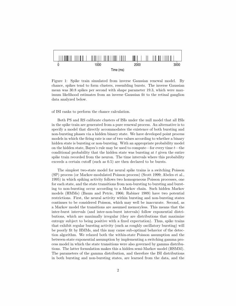
Some authors have devised extracellular burst-detection methods based oninterspike interval (ISI) length, often with a criterion for a minimal number ofspikes with small ISIs (Lo et al., 1991; Martinson et al., 1997; Corner et al.,2002; Turnbull et al., 2005; Tam, 2002). A conceptual difficulty for such meth-ods, illustrated in Figure 1, is that spike trains generated from pure renewalprocesses—such as those produced by simple integrate-and-fire models—canexhibit clusters of neurons that have the appearance of bursts. In some circum-stances these “null cases” might be ruled out by substantive considerations. Inmost others, one needs a careful, model-based calibration to determine whetheror not a cluster of short ISIs represents a burst.

A very popular burst-detection method, called Poisson Surprise (PS) (Leg-endy and Salcman, 1985), offers such a calibration based on a probabilisticmodel on the ISIs. With PS, one calculates a surprise value S to measure howunlikely it is that a cluster with n spikes in a time interval T , would occur bychance. The method performs its chance calculation under the assumption thatthe ISIs are independent realizations from an exponential density. This amountsto assuming the neuron to spike according to a time homogeneous Poisson pro-cess. It is, however, known that spike trains often exhibit distinctly non-Poissonbehavior (Koch, 2004; Gourevitch and Eggermont, 2007). To avoid the Poissonassumption Gourevitch and Eggermont (2007) proposed a rank surprise (RS)index, which again computes a surprise value but instead uses the distribution

1

Time (ms)

0 1000 2000 3000

Figure 1: Spike train simulated from inverse Gaussian renewal model. Bychance, spikes tend to form clusters, resembling bursts. The inverse Gaussianmean was 30.8 spikes per second with shape parameter 19.3, which were max-imum likelihood estimates from an inverse Gaussian fit to the retinal gangliondata analyzed below.

of ISI ranks to perform the chance calculation.

Both PS and RS calibrate clusters of ISIs under the null model that all ISIsin the spike train are generated from a pure renewal process. An alternative is tospecify a model that directly accommodates the existence of both bursting andnon-bursting phases via a hidden binary state. We have developed point processmodels in which the firing rate is one of two values according to whether a binaryhidden state is bursting or non-bursting. With an appropriate probability modelon the hidden state, Bayes’s rule may be used to compute—for every time t—theconditional probability that the hidden state was bursting at t given the entirespike train recorded from the neuron. The time intervals where this probabilityexceeds a certain cutoff (such as 0.5) are then declared to be bursts.

The simplest two-state model for neural spike trains is a switching Poisson(SP) process (or Markov-modulated Poisson process) (Scott 1999; Abeles et al.,1995) in which spiking activity follows two homogeneous Poisson processes, onefor each state, and the state transitions from non-bursting to bursting and burst-ing to non-bursting occur according to a Markov chain. Such hidden Markovmodels (HMMs) (Baum and Petrie, 1966; Rabiner 1989) have two potentialrestrictions. First, the neural activity within bursting and non-bursting statescontinues to be considered Poisson, which may well be inaccurate. Second, asa Markov model the transitions are assumed memoryless. This means that theinter-burst intervals (and inter-non-burst intervals) follow exponential distri-butions, which are maximally irregular (they are distributions that maximizeentropy subject to being positive with a fixed expectation). Thus, spike trainsthat exhibit regular bursting activity (such as roughly oscillatory bursting) willbe poorly fit by HMMs, and this may cause sub-optimal behavior of the detec-tion algorithm. We relaxed both the within-state Poisson assumption and thebetween-state exponential assumption by implementing a switching gamma pro-cess model in which the state transitions were also governed by gamma distribu-tions. The latter formulation makes this a hidden semi-Markov model (HSMM).The parameters of the gamma distribution, and therefore the ISI distributionsin both bursting and non-bursting states, are learned from the data, and the

2

bursting and non-bursting state transitions are estimated. The purpose of thisarticle is to describe our HSMM implementation and study its effectiveness.

An appealing feature of HMMs is computational tractability, most often viaan expectation-maximization algorithm known as the Baum-Welch algorithm.This algorithm uses a fast forward-backward recursion to perform maximumlikelihood estimation of model parameters and conditional probability evalua-tion of the hidden state given the estimated parameters. Chib (1996) developeda variation of this to construct a Markov Chain Monte Carlo (MCMC) algorithmfor a Bayesian treatment of this model. In the Bayesian setting, the conditionalprobability evaluation requires an additional integration over the model param-eters with respect to their joint posterior distribution given the observed spiketrain. Chib (1996) noted that the Markov chain structure of the HMM modelallows efficient sampling from the posterior distribution through a Gibbs sam-pler. The computational approach we have developed applies Gibbs samplingto HSMMs by expanding the state space so that the HSMM takes a Markovianform. In Section 2 we provide details of our implementation; in Section 3 wegive results from a small simulation study, comparing our HSMM to PS and RS,and also to a point-process HMM; in Section 4 we apply the HSMM to a dataset analyzed previously by several other authors; and in Section 5 we discussthe results.

2 Methods

2.1 Hidden Binary Model

We denote the hidden binary state of the neuron at time t by C(t) with C(t) =1 coding a bursting state, C(t) = 0 a non-bursting state. We suppose theobservation time interval is [0, T ] and assume that on this interval C(t) canhave only finitely many transitions between its two states. The waiting timefrom one transition to the next will be called an inter-transition interval (ITI).The ITIs are assumed independent. Those corresponding to the bursting state(C(t) = 1) are from a density f ITI

1 (·) and those from a non-bursting state arefrom a density f ITI

0 (·).

Within each state, we consider the neural spike train to be governed by arenewal process with an inter-spike interval (ISI) probability density f1 or f0depending on the state level. Such a conception may be technically inaccuratebecause transitions may occur in the midst of an ISI. However, for simplicity weassume that every ISI is regulated by the state of the neuron at the completionof the previous spike. (As we mention in the discussion, we also investigated analternative method that did not make this assumption, but it was much morecumbersome and gave similar results in the cases we examined.) More formally,

3

letting yi be the i-th ISI and τi =∑ij=1 yj denote the time of the i-th spike, the

first ISI Y1 is assumed to follow f ISIC(0) and the subsequent ISI’s are conditionally

modeled as:yi | (y1, · · · , yi−1, C[0, τi−1]) ∼ f ISI

C(τi−1)(1)

with C[0, T ] = {C(t) : 0 ≤ t ≤ T}. Each of the four densities f ITIs , f ISI

s ,s ∈ {0, 1} is assumed known only up to finitely many parameters, all of whichare collected together into a vector θ. In addition to the hidden binary burststates, the vector θ must be learned from the data.

2.2 Burst Detection

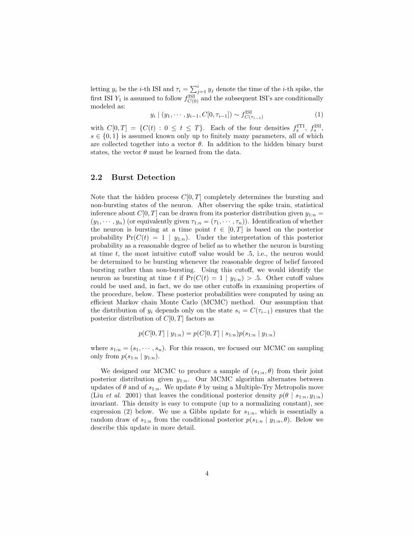
Note that the hidden process C[0, T ] completely determines the bursting andnon-bursting states of the neuron. After observing the spike train, statisticalinference about C[0, T ] can be drawn from its posterior distribution given y1:n =(y1, · · · , yn) (or equivalently given τ1:n = (τ1, · · · , τn)). Identification of whetherthe neuron is bursting at a time point t ∈ [0, T ] is based on the posteriorprobability Pr(C(t) = 1 | y1:n). Under the interpretation of this posteriorprobability as a reasonable degree of belief as to whether the neuron is burstingat time t, the most intuitive cutoff value would be .5, i.e., the neuron wouldbe determined to be bursting whenever the reasonable degree of belief favoredbursting rather than non-bursting. Using this cutoff, we would identify theneuron as bursting at time t if Pr(C(t) = 1 | y1:n) > .5. Other cutoff valuescould be used and, in fact, we do use other cutoffs in examining properties ofthe procedure, below. These posterior probabilities were computed by using anefficient Markov chain Monte Carlo (MCMC) method. Our assumption thatthe distribution of yi depends only on the state si = C(τi−1) ensures that theposterior distribution of C[0, T ] factors as

p(C[0, T ] | y1:n) = p(C[0, T ] | s1:n)p(s1:n | y1:n)

where s1:n = (s1, · · · , sn). For this reason, we focused our MCMC on samplingonly from p(s1:n | y1:n).

We designed our MCMC to produce a sample of (s1:n, θ) from their jointposterior distribution given y1:n. Our MCMC algorithm alternates betweenupdates of θ and of s1:n. We update θ by using a Multiple-Try Metropolis move(Liu et al. 2001) that leaves the conditional posterior density p(θ | s1:n, y1:n)invariant. This density is easy to compute (up to a normalizing constant), seeexpression (2) below. We use a Gibbs update for s1:n, which is essentially arandom draw of s1:n from the conditional posterior p(s1:n | y1:n, θ). Below wedescribe this update in more detail.

4

2.3 Sampling from p(s1:n | y1:n, θ)

Given θ, the pair (s1:n, y1:n) defines a hidden Markov model when f ITI1 and f ITI

0

are exponential densities. This results in the property that C(t, T ] is condition-ally independent of C[0, t) given C(t) for any 0 ≤ t < T , which ensures thatthe si’s form a Markov chain. For such models where the si’s live on a finitestate space, Chib (1996) developed an efficient algorithm to sample from theposterior distribution of s1:n given Y1:n. He introduced a Gibbs sampler thatsampled all of s1:n in a single draw, which made the procedure much faster thanMetropolis-Hastings samplers where the hidden states were updated one at atime.

Chib’s method, however, relies on the Markov property of s1:n and thus doesnot apply to the case where f ITI

1 and f ITI0 are not exponential densities. We

have introduced a suitable variable augmentation which induces the requiredMarkov property on an extended state space. The basic idea is to archive withevery spike time τi the time since the last transition. Although this time cannotbe exactly determined from y1:n and s1:n, it can be bracketed by (ri − yi, ri)where

ri = yi−mi+1 + · · ·+ yi

with mi = min{j > 0 : si−j 6= sj}. If we restrict C(t) from having more thanone transition between two successive spikes, then

p(s1:n, y1:n | θ) = p(s1)f ISIs1 (y1)

n∏j=2

Bernoulli(I(si = si−1) | φsi−1,ri−1,yi−1) (2)

where Bernoulli(x | p) = px(1− p)1−x denotes a Bernoulli pdf with probabilityp, I(·) denotes the indicator function and φs,r,y = (1−F ITI

s (r))/(1−F ITIs (r−y))

is the probability that an ITI in state s will stretch beyond r given that it isalready larger than r − y; here F ITI

0 and F ITI1 are the cumulative distribution

functions corresponding to f ITI0 and f ITI

1 . With these definitions (si, ri, yi) formsa Markov chain with the distribution of s1 = C(0) unspecified.

We now present details of our adaptation of Chib’s method to sample fromp(s1:n, r1:n | y1:n, θ) where r1:n = (r1, · · · , rn). In the following we suppress θfrom the notations, because all computations are done for θ fixed at its currentvalue in the MCMC. The following notations and derivations closely follow theconstructions given in Chib (1996). For any vector x1:n = (x1, · · · , xn), let xi:jdenote the sub-vector (xi, xi+1, · · · , xj), 1 ≤ i ≤ j ≤ n. Notice that

p(s1:n, r1:n | y1:n) = p(sn, rn | y1:n)n−1∏i=1

p(si, ri | si+1:n, ri+1:n, y1:n)

with

p(si, ri | si+1:n, ri+1:n, y1:n) ∝ p(yi+1:n, si+1:n, ri+1:n | si, ri, y1:i)p(si, ri | y1:i)∝ p(yi+1, si+1, ri+1 | si, ri)p(si, ri | y1:i).

5

Because r1:i is always completely determined by y1:i and s1:i, the first probabilitydistribution above can be written as

p(yi+1, si+1, ri+1 | si, ri) =I(ri+1 = I(si+1 = si)ri + yi+1)p(si+1, yi+1 | si, ri).

Therefore, once the pdfs p(si, ri | y1:i) are known, (s1:n, r1:n) can be easilysampled from p(s1:n, r1:n | y1:n) by sequentially sampling (sn, rn), (sn−1, rn−1)and so on. Below we outline how these pdfs can be computed in a recursivemanner—this again follows the strategy in Chib (1996) but with some importantdifferences.

Let lij = yi + yi−1 + · · · + yi−j+1, i = 1, · · · , n and j = 1, · · · , i. It isclear that the i-th pdf gi(si, ri) = p(si, ri | y1:i) is to be evaluated only at(si, ri) ∈ {0, 1} × {lij ; j = 1, 2, · · · , i}. Suppose these evaluations have beendone for a given i. Then the next pdf gi+1(si+1, ri+1) can be evaluated at thedesired values via the following two steps:

1. Prediction:

p(si+1 = 1, ri+1 = li+1,1 | y1:i)

=i∑

j=1

gi(si = 0, ri = lij)Bernoulli(1 | φ(0, lij))f(yi+1 | λ(1, 0, lij , θ))

p(si+1 = 0, ri+1 = li+1,1 | y1:i)

=i∑

j=1

gi(si = 1, ri = lij)Bernoulli(0 | φ(1, lij))f(yi+1 | λ(0, 1, lij , θ))

p(si+1 = 1, ri+1 = li+1,j | y1:i)= gi(si = 1, ri = li,j−1)Bernoulli(1 | φ(1, li,j−1))f(yi+1 | λ(1, 1, li,j−1))p(si+1 = 0, ri+1 = li+1,j | y1:i)

= gi(si = 0, ri = li,j−1)Bernoulli(0 | φ(0, li,j−1))f(yi+1 | λ(0, 0, li,j−1))

2. Update:

gi+1(si+1, ri+1) =p(si+1, ri+1 | y1:i)

ci+1

where

ci+1 =1∑k=0

i+1∑j=1

p(si+1 = k, ri+1 = li+1,j | y1:i).

The algorithm described above demands O(n2) flops and storage. This canbe reduced to O(n) by splitting the spike train into contiguous segments and

6

updating the states of the ISI’s within each segment together. Choosing thesesegments to be of length O(w), the entire train can be updated with only O(nw)flops and storage. In our examples we chose the segment length randomly froma discrete uniform distribution on the integers in [5; 20]. The segments arecreated and processed from right to left until the whole train is covered. Noticethat choosing the window length as large as n would be practically infeasibleexcept for very small spike trains. On the other hand choosing the window tooshort would resemble the less inefficient one-state-at-a-time update.

3 Simulation Study

After implementing the HSMM described above we assessed its performance,comparing it to HMM, PS and RS. For our comparisons we used spike trainssimulated from 5 distinct processes, which we call settings, chosen to combinerealistic ISI distributions together with features that might pose a challenge tothe methods. We then evaluated the methods based on estimated number ofbursts and ROC curves.

Each setting corresponded to a model that was likely to produce clustersof small ISIs purely by chance in addition to, and in one case dominating, ahidden binary process C(t) having moderate regularity in its transitions. Thefirst setting was the “null” setting illustrated in Figure 1; the second and thirdsettings were inverse Gaussian and gamma switching processes with the ISI dis-tributions either largely overlapping (setting 2) or clearly separated (setting 3)under the bursting and non-bursting states; the fourth setting produced non-bursting state ISIs from a mixture model, which is different than the HSMMand might confuse a burst detection algorithm; the fifth setting used an expo-nential distribution for the down-state durations, which makes the inter-burstdurations maximally irregular and state identification more difficult to detect.More specifically, the processes we considered were as follows:

1. (Null.) Here we set C(t) = 0 for all t ∈ [0, T ]. We generated spike trainsfrom a pure renewal process with ISI distribution f ISI

0 given by an inverseGaussian with shape 19.33 and mean 30.76, as in Figure 1.

2. (IGovlp.) The hidden state C(t) follows a switching gamma process withf ITI1 = Gamma(10, 10/(25ms)) and f ITI

0 = Gamma(10, 10/(200ms)). Wechose the average duration of 25ms for an bursting state and 200ms for anon-bursting state according to the HSMM fit to the goldfish data. Thebursting state ISIs were simulated from f ISI

1 = Gamma(20, 20/(7ms)).Our fit to the retinal ganglion data (described below) provided the choiceof 7ms as the average bursting state length. We generated the non-bursting state ISIs according to the inverse Gaussian distribution of theNull process described above.

7

3. (IGsep.) Same as IGovlp but we instead generated the down state ISIsfrom an inverse Gaussian distribution with shape 150 and mean 50ms.This choice ensured that the two ISI distributions were well separated—-the shortest non-bursting state ISIs were likely to be considerably largerthan most bursting state ISIs.

4. (Gmix.) Same as IGovlp but we instead generated the down state ISIsfrom the mixture (2/3)Gamma(10, 10/(10ms))+(1/3)Gamma(10, 10/(75ms)).The first component of the mixture had a substantial overlap with f ISI

1 .

5. (IGirr.) Same as the IGsep setting but we instead generated the non-bursting state ITI of C(t) from f ITI

0 = Exponential(1/(200ms)) distribu-tion. Thus C(t) was memoryless during the down state.

In all cases the spike trains were 10s in duration, with about 500 spikes perrecord on average.

We implemented HSMM burst detection with a switching gamma modelgiven by

f ISI0 = Gamma(α0, α0/µ0)f ISI1 = Gamma(α1, α1/µ1)f ITI0 = Gamma(15, 15/λ0)f ITI0 = Gamma(15, 15/λ1)

with θ = (α0, α1, µ0, µ1, λ0, λ1). We modeled the ISI shapes α0 and α1 witha log-normal prior: logαi ∼ Normal(log(10), 12). Similarly, we modeled theISI means (in ms) as logµi ∼ Normal(log(20), 22) and the ITI means (in ms)as log λi ∼ Normal(log(100), 42). We first obtained an MCMC estimate to theburst probability pi = Pr(si = 1 | y1:n) for each ISI. We labeled each ISI withsi = 1 if pi was at least as large as a chosen cutoff level, and 0 otherwise.We considered each contiguous string of states with si = 1 to be a burst. Anestimate of the time the neuron spent in the bursting state is the sum of theISIs with si = 1. Cutoffs used were 0.00, 0.01, · · · , 1.00, 1.01.

We implemented HMM burst detection by modifying the HSMM algorithmdescribed above so that f ITI

i = Exponential(1/λi), i = 0, 1. Note that this HMMis more general than the switching Poisson process model because it allows non-Poisson firing within burst and non-burst periods. We implemented the PS andRS methods via the exhaustive surprise maximization (EMS) search techniqueof Gourevitch and Eggermont (2007) with a chosen surprise cutoff − log(α)with α in {0.001, 0.005, 0.01, 0.05, 0.1, 0.15, 0.2, 0.3, 0.4, 05}. To maintain paritybetween all four methods, we did not count the bursts made of a single ISI andtruncated f ISI

0 at the 75-th percentile of the observed ISI values. Both theselimits are hard coded in the EMS implementation of Gourevitch and Eggermont(2007).

8

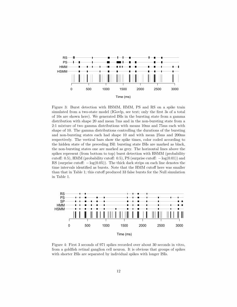
To evaluate burst count accuracy of the 4 methods we assessed the rootmean squared error (RMSE). Each method requires a choice of cutoff, and eachmethod will falsely identify some non-burst clusters of spikes as bursts. Tomake the methods comparable, we started with the null model, where thereare no bursts, and picked cutoff values that produced roughly the same numberof (false) bursts for each method; we then assessed the ability of the methodsto track burst counts for the remaining 4 settings, where bursts were trulypresent—this is analogous to the standard statistical practice of fixing type Ierror and then examining power. Results are given in Table 1. In each of thenon-null settings, the RMSE for HSMM was much smaller than those for PS andRS. HSMM and HMM had similar results except in the cases IGovlp and Gmix,where the RMSE for HMM was about 3 times larger than that for HSMM.Figure 3 shows a visual summary of burst detection by all four methods on asimulated spike train.

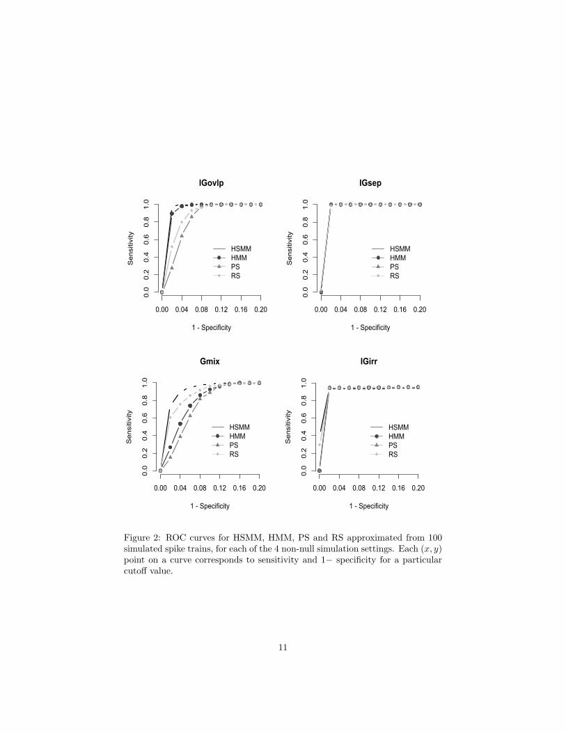
Comparisons of the type given in Table 1 are important but, because thecutoffs were fixed according to null-setting performance, they are only part ofthe story. We examined all methods across a range a cutoffs using ROC curves.For each method, for a set of cuttoffs, we evaluated both sensitivity (proportionof time in bursting state correctly identified) and specificity (proportion of timein non-bursting state correctly identified). For every method, as the cutoff isincreased bursts become harder to detect, so that the specificity increases andthe sensitivity decreases. The ROC curve plots sensitivity on the y-axis and 1−specificity on the x-axis. An optimal ROC curve begins at the origin, hugs they-axis up to (0,1), and then moves to the point (1,1) along the line y = 1. ROCcurves for the 4 methods in the 4 non-null settings are displayed in Figure 2.

We draw three general conclusions from the ROC analysis. First, HSMMperforms as well as the other methods, and for the IGovlp and Gmix settings itperforms better; the curves for HSMM were generally to the left of the others,meaning that HSMM was much more specific, spending significantly less timefalsely identifying bursting states; and the curves for HSMM were also generallyabove those for the other methods, meaning that HSMM was generally spendingmore of the time correctly identifying bursting states. Second, in some cases PSand RS with particular cutoffs performed well, with RS outperforming PS inthe IGovlp and Gmix settings, where the 4 methods clearly differed. However,it should be noted that a key feature of these curves is their upper left-mostpoint, which is obtained for a particular “optimal” cutoff, and that cutoffs nearthis optimal cutoff have generally good sensitivity and specificity. Such cutoffsthat allowed PS and RS to perform well in some settings produced unreliableresults in other simulation settings. In the Null case we found that the abilityof any method to handle false burstiness depends crucially on the cutoffs. Thus,in particular, in the last case, IGirr, which had memoryless switching fromnon-bursting to bursting state, all methods performed well according to thecurves in Figure 2; but the cutoff values for which RS and PS attained the goodsensitivity and specificity in IGirr were much smaller than those that would

9

Setting HSMM HMM PS RSNull (0) 15 14 14 14

IGovlp (38) 1 3 10 14IGsep (38) 0 1 4 16Gmix (38) 8 23 8 15IGirr (81) 5 3 106 88

Table 1: Root mean squared error (RMSE) of estimated burst counts accordingto 5 distinct model settings (first column). One hundred simulated spike trainswere used for every setting. For all settings the average true burst counts aregiven in parentheses. To ensure the methods were comparable under the nullsetting, we used probability cutoffs of 0.5 for HSMM and 0.8 for HMM, andsurprise cutoffs of − log(0.01) for PS and − log(0.05) for RS.

typically provide good performance in the Null setting. Third, in Gmix, whichwe designed to contradict the assumptions of the HSMM (the HSMM could notpossibly provide fit the bimodal f ISI

0 because it is based on a unimodal gammadensity), the HSMM performed extremely well.

One additional point worth mentioning is that the HMM usually produceda nice fit to the ISI histogram for the spike trains generated under Gmix. Thereason is that the non-burst ISI distribution from the first component of themixture was similar to the burst ISI distribution—and the HMM identified bothkinds of ISIs as burst ISIs. Consequently, it did a poor job of burst detectionbut that was not apparent from its fit to the ISI histogram. In general, goodnessof fit can not be judged solely from a fit to the ISI histogram.

4 Data Analysis

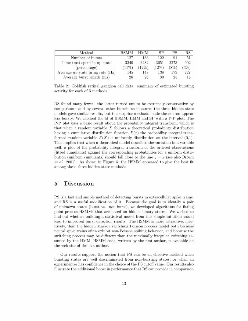
To illustrate our proposed method on real data we use a spike train recordedfrom a goldfish retinal ganglion cell neuron in vitro (Brown et al. 2004; Levine1991; Iyengar and Liao 1997). The data include 971 spikes recorded over about30 seconds. The plot of the spikes from this neuron in Figure 4 shows some ap-parent clusters of spikes with shorter intervals, and these clusters are separatedby spikes with longer intervals between them.

We analyzed this spike train with HSMM, HMM, PS, RS as well as withthe switching Poisson (SP) model which is a special case of HMM with theshape parameters of the ISI densities fixed at 1. The cutoffs were probability.5 for HSMM, HMM, and SP, and surprise − log .01 for PS and − log 0.05 forRS. Based on the simulations reported above, we would expect HSMM to bethe most accurate, and the question remains whether the methods are appre-ciably different for this data set. HSMM found 127 bursts, whereas PS and

10

0.0

0.2

0.4

0.6

0.8

1.0

0.00 0.04 0.08 0.12 0.16 0.20

HSMMHMMPSRS

IGovlp

1 - Specificity

Sensitivity

0.0

0.2

0.4

0.6

0.8

1.0

0.00 0.04 0.08 0.12 0.16 0.20

HSMMHMMPSRS

IGsep

1 - Specificity

Sensitivity

0.0

0.2

0.4

0.6

0.8

1.0

0.00 0.04 0.08 0.12 0.16 0.20

HSMMHMMPSRS

Gmix

1 - Specificity

Sensitivity

0.0

0.2

0.4

0.6

0.8

1.0

0.00 0.04 0.08 0.12 0.16 0.20

HSMMHMMPSRS

IGirr

1 - Specificity

Sensitivity

Figure 2: ROC curves for HSMM, HMM, PS and RS approximated from 100simulated spike trains, for each of the 4 non-null simulation settings. Each (x, y)point on a curve corresponds to sensitivity and 1− specificity for a particularcutoff value.

11

Time (ms)

HSMM

HMM

PS

RS

0 500 1000 1500 2000 2500 3000

Figure 3: Burst detection with HSMM, HMM, PS and RS on a spike trainsimulated from a two-state model (IGovlp, see text; only the first 3s of a totalof 10s are shown here). We generated ISIs in the bursting state from a gammadistribution with shape 20 and mean 7ms and in the non-bursting state from a2:1 mixture of two gamma distributions with means 10ms and 75ms each withshape of 10. The gamma distributions controlling the durations of the burstingand non-bursting states each had shape 10 and with mean 25ms and 200msrespectively. The vertical bars show the spike times, color coded according tothe hidden state of the preceding ISI: bursting state ISIs are marked as black,the non-bursting states one are marked as grey. The horizontal lines above thespikes represent (from bottom to top) burst detection with HSMM (probabilitycutoff: 0.5), HMM (probability cutoff: 0.5), PS (surprise cutoff: − log(0.01)) andRS (surprise cutoff: − log(0.05)). The thick dark strips on each line denotes thetime intervals identified as bursts. Note that the HMM cutoff here was smallerthan that in Table 1; this cutoff produced 33 false bursts for the Null simulationin Table 1.

Time (ms)

HSMM

HMM

SP

PS

RS

0 500 1000 1500 2000 2500 3000

Figure 4: First 3 seconds of 971 spikes recorded over about 30 seconds in vitro,from a goldfish retinal ganglion cell neuron. It is obvious that groups of spikeswith shorter ISIs are separated by individual spikes with longer ISIs.

12

Method HSMM HMM SP PS RSNumber of bursts 127 133 122 91 51

Time (ms) spent in up state 3240 3482 3651 2273 902(percentage) (11%) (12%) (12%) (8%) (3%)

Average up state firing rate (Hz) 145 148 138 173 227Average burst length (ms) 26 26 30 25 18

Table 2: Goldfish retinal ganglion cell data: summary of estimated burstingactivity for each of 5 methods.

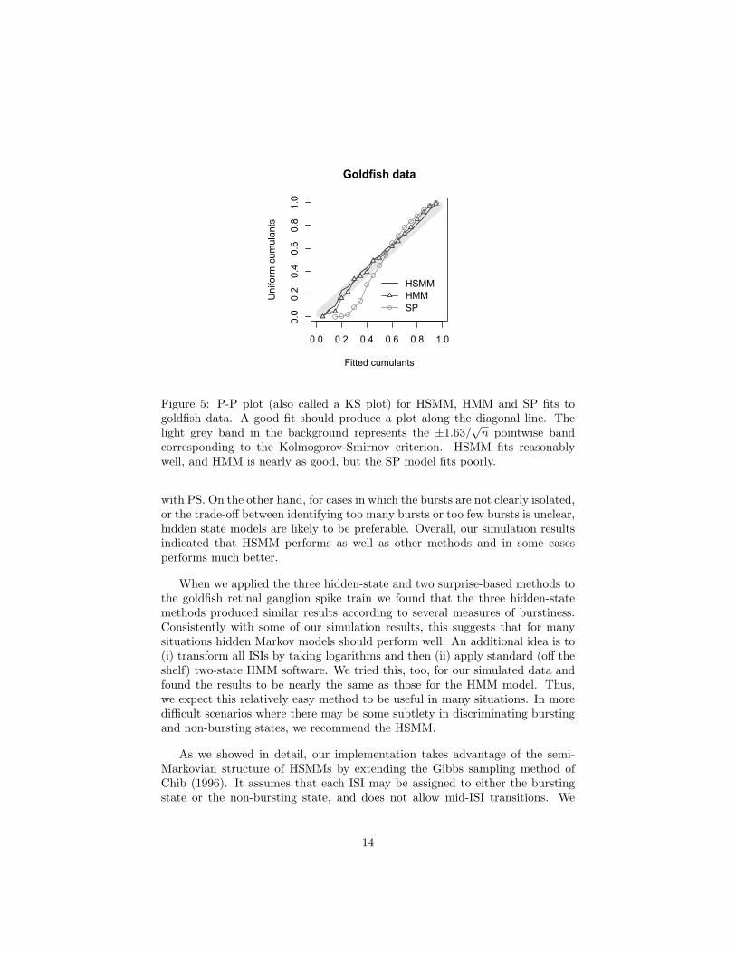
RS found many fewer—the latter turned out to be extremely conservative bycomparison—and by several other burstiness measures the three hidden-statemodels gave similar results, but the surprise methods made the neuron appearless bursty. We checked the fit of HSMM, HMM and SP with a P-P plot. TheP-P plot uses a basic result about the probability integral transform, which isthat when a random variable X follows a theoretical probability distributionhaving a cumulative distribution function F (x) the probability integral trans-formed random variable F (X) is uniformly distribution on the interval (0,1).This implies that when a theoretical model describes the variation in a variablewell, a plot of the probability integral transform of the ordered observations(fitted cumulants) against the corresponding probabilities for a uniform distri-bution (uniform cumulants) should fall close to the line y = x (see also Brownet al. 2001). As shown in Figure 5, the HSMM appeared to give the best fitamong these three hidden-state methods.

5 Discussion

PS is a fast and simple method of detecting bursts in extracellular spike trains,and RS is a useful modification of it. Because the goal is to identify a pairof unknown states (burst vs. non-burst), we developed algorithms for fittingpoint-process HSMMs that are based on hidden binary states. We wished tofind out whether building a statistical model from this simple intuition wouldlead to improved burst detection results. The HSMM is more attractive, intu-itively, than the hidden Markov switching Poisson process model both becauseneural spike trains often exhibit non-Poisson spiking behavior, and because theswitching process may be different than the maximally irregular switching as-sumed by the HMM. HSMM code, written by the first author, is available onthe web site of the last author.

Our results support the notion that PS can be an effective method whenbursting states are well discriminated from non-bursting states, or when anexperimenter has confidence in the choice of the PS cutoff value. Our results alsoillustrate the additional boost in performance that RS can provide in comparison

13

0.0 0.2 0.4 0.6 0.8 1.0

0.0

0.2

0.4

0.6

0.8

1.0

HSMMHMMSP

Goldfish data

Fitted cumulants

Uni

form

cum

ulan

ts

Figure 5: P-P plot (also called a KS plot) for HSMM, HMM and SP fits togoldfish data. A good fit should produce a plot along the diagonal line. Thelight grey band in the background represents the ±1.63/

√n pointwise band

corresponding to the Kolmogorov-Smirnov criterion. HSMM fits reasonablywell, and HMM is nearly as good, but the SP model fits poorly.

with PS. On the other hand, for cases in which the bursts are not clearly isolated,or the trade-off between identifying too many bursts or too few bursts is unclear,hidden state models are likely to be preferable. Overall, our simulation resultsindicated that HSMM performs as well as other methods and in some casesperforms much better.

When we applied the three hidden-state and two surprise-based methods tothe goldfish retinal ganglion spike train we found that the three hidden-statemethods produced similar results according to several measures of burstiness.Consistently with some of our simulation results, this suggests that for manysituations hidden Markov models should perform well. An additional idea is to(i) transform all ISIs by taking logarithms and then (ii) apply standard (off theshelf) two-state HMM software. We tried this, too, for our simulated data andfound the results to be nearly the same as those for the HMM model. Thus,we expect this relatively easy method to be useful in many situations. In moredifficult scenarios where there may be some subtlety in discriminating burstingand non-bursting states, we recommend the HSMM.

As we showed in detail, our implementation takes advantage of the semi-Markovian structure of HSMMs by extending the Gibbs sampling method ofChib (1996). It assumes that each ISI may be assigned to either the burstingstate or the non-bursting state, and does not allow mid-ISI transitions. We

14

also explored an alternative method that does allow mid-ISI transitions, alongthe general lines used by Scott (1999) for switching Poisson process models. Wefound that in practice this alternative approach did not produce greatly differentresults, and we therefore preferred to present the more computationally efficientmethod. For convenience we used gamma distributions to describe both ISIs andITIs. We would expect that in most cases, replacing gammas with alternativetwo-parameter families, or introducing more general families, would not have alarge impact on results. However, the algorithm we described was formulatedto allow such further generality. It is also possible that faster methods basedon EM-type algorithms may be possible based on the same general idea ofexploiting the Markovian structure inherent in these HSMMs. This is a topicfor future research.

References

Abeles, M., Bergman, H., Gat, I., Meilijson, I., Seidemann, E., Thishby, N.,Vaadia, E. (1995), Cortical activity flips among quasi stationary states, Proc.Nat. Acad. Sci., 92: 8616-8620.

Baum, L. E. and Petrie, T. (1966), Statistical Inference for probabilisticfunctions of finite state Markov chains, Ann. Math. Stat., vol. 37, pp. 1554–1563.

Brown, E. N., Barbieri, R., Eden, U. T., and Frank, L. M. (2004), LikelihoodMethods for Neural Spike Train Data Analysis, in Computational Neuroscience:A Comprehensive Approach, edited by Jianfeng Feng, CRC Press, pp.253-286.

Brown, B.N., Barbieri, R, Ventura V., Kass, R.E., and Frank, L.M. (2002),The time -rescaling theorem and its applications to neural spike train dataanalysis, Neural Computation, 14: 325–346.

Chen, Z., Vijayan, S., Barbieri, R., Wilson, M.A., Brown, E. N. (2008),Discrete- and continuous-time probabilistic models and inference algorithms forneuronal decoding of up and down states, submitted.

Chib, S. (1996), Calculating posterior distributions and modal estimates inMarkov mixture models, Journal of Econometrics, 75: 79-97.

Cooper, D.C., Chung, S., Spruston, N. (2005), Output-Mode TransitionsAre Controlled by Prolonged Inactivation of Sodium Channels in PyramidalNeurons of Subiculum, PLoS Biology, Vol. 3, pp. 1123-1129.

Corner, M.A., van Pelt, J., Wolters, P.S., Baker, R.E., and Nuytinck, R.H.(2002), Physiological effects of sustained blockade of excitatory synaptic trans-

15

mission on spontaneously active developing neuronal networks-an inquiry intothe reciprocal linkage between intrinsic biorhythms and neuroplasticity in earlyontogeny, Neurosci Biobehav Rev, 26: 127-185.

Doiron, B., Chacron, M.J., Maler, L., Longtin, A., Bastian, J. (2003), In-hibitory feedback required for network oscillatory responses to communicationbut not prey stimuli. Nature, 421:539-543.

Gerkin, R.C., Yassin, K., Clem, R.L., Shruti, S., Kass, R.E., Barth, A.L.(2008), Seizure-dependent changes in cortical output: evaluation using an adap-tive threshold for the detection of state changes in intracellular recordings, sub-mitted to Journal of Computational Neuronscience.

Gourevitch, B., Eggermont, J. J. (2007), A nonparametric approach fordetection of bursts in spike trains, Journal of Neuroscience Methods, 160:349-358.

Iyengar, S., and Liao, Q. (1997). Modeling neural activity using the gener-alized inverse Gaussian distribution. Biol. Cyber., 77, 289-295.

Izhikevich, E.M., Desai, N.S., Walcott, E.C., Hoppensteadt, F.C. (2003),Bursts as a unit of neural information: selective communication via resonance.Trends in Neuroscience, 26:161-167.

Koch, C., Biophysics of Computation: Information Processing in Single Neu-rons, Oxford University Press: New York, 2004.

Legendy, C. R. and Salcman, M. (1985), Bursts and recurrences of burstsin the spike trains of spontaneously active striate cortex neurons, Journal ofNeurophysiology, 53: 926-939.

Levine, M.W. (1991). The distribution of intervals between neural impulsesin the maintained discharges of retinal ganglion cells. Biol. Cybern., 65: 459-467.

Liu, J. S., Liang, F. and Wong. W. H. (2000). The use of multiple-trymethod and local optimization in Metropolis sampling, Journal of the AmericanStatistical Association, 96(454): 561-573.

Lo, F.-S., Lu, S.-M., and Sherman, S. M. (1991), Intracellular and extra-cellular in vivo recording of different response modes for relay cells of the cat’slateral geniculate nucleus. Exp. Brain Rex 83: 3 17-328.

Martinson, J., Webster, H., Myasnikov, A., and Dykes, W. (1997), Recog-nition of temporaly structured activity in spontaneously discharging neurons inthe somatosensory cortex in waking cats, Brain Res 750:129-140.

16

Rabiner, L.R. (1989), A Tutorial on hidden Markov modelss and SelectedApplications in Speech Recognition, Proceedings of the IEEE, 77 (2), pp. 257-286.

Scott, S. L.(1999), Bayesian Analysis of a Two-State Markov ModulatedPoisson Process, Journal of Computational and Graphical Statistics, 8: 662-670.

Tam, D. C. (2002). An alternate burst analysis for detecting intra-burstfirings based on inter-burst periods, Neurocomputing, 44-46 (C): 1155-1159.

Turnbull, L., Gross, G.. W. (2005), The string method of burst identificationin neuronal spike trains, Journal of Neuroscience Methods, 145: 23-35.

Wilson, H.R., Cowan, J.D. (1972) Excitatory and inhibitory interactions inlocalized populations of model neurons, Biophys. J., 12:1-24.

17