Detecting Stable Clusters Using Principal Component …asa/pdfs/pcachap.pdfPrincipal Component...

A. Ben-Hur and I. Guyon. Detecting stable clusters using principal component analysis. In Functional Genomics:Methods and Protocols. M.J. Brownstein and A. Kohodursky (eds.) Humana press, 2003 pp. 159-182

Detecting Stable Clusters UsingPrincipal Component Analysis

Asa Ben-Hur and Isabelle Guyon

1 Introduction

Clustering is one of the most commonly used tools in the analysis of gene expressiondata(1, 2). The usage in grouping genes is based on the premise that co-expression isa result of co-regulation. It is thus a preliminary step in extracting gene networks andinference of gene function(3, 4). Clustering of experiments can be used to discover novelphenotypic aspects of cells and tissues(3, 5, 6), including sensitivity to drugs(7), andcan also detect artifacts of experimental conditions(8). Clustering and its applications inbiology are presented in greater detail in the chapter by Zhao and Karypis (see also(9)).While we focus on gene expression data in this chapter, the methodology presented here isapplicable for other types of data as well.

Clustering is a form of unsupervised learning, i.e. no information on the class variableis assumed, and the objective is to find the “natural” groups in the data. However, mostclustering algorithms generate a clustering even if the data has no inherent cluster structure,so external validation tools are required. Given a set of partitions of the data into an in-creasing number of clusters (e.g. by a hierarchical clustering algorithm, or k-means), sucha validation tool will tell the user the number of clusters inthe data (if any). Many methodshave been proposed in the literature to address this problem(10–15). Recent studies haveshown the advantages of sampling-based methods(12, 14). These methods are based onthe idea that when a partition has captured the structure in the data, this partition should bestable with respect to perturbation of the data. Bittneret al. (16) used a similar approachto validate clusters representing gene expression of melanoma patients.

The emergence of cluster structure depends on several choices: data representationand normalization, the choice of a similarity measure and clustering algorithm. In thischapter we extend the stability-based validation of cluster structure, and propose stabilityas a figure of merit that is useful for comparing clustering solutions, thus helping in makingthese choices. We use this framework to demonstrate the ability of Principal ComponentAnalysis (PCA) to extract features relevant to the cluster structure. We use stability as atool for simultaneously choosing the number of principal components and the number ofclusters; we compare the performance of different similarity measures and normalizationschemes. The approach is demonstrated through a case study of yeast gene expression datafrom Eisenet al. (1). For yeast, a functional classification of a large number of genes isknown, and we use this classification for validating the results produced by clustering. Amethod for comparing clustering solutions specifically applicable to gene expression datawas introduced in(17). However, it cannot be used to choose the number of clusters,andis not directly applicable in choosing the number of principal components.

The results of clustering are easily corrupted by the addition of noise: even a few

1


noise variables can corrupt a clear cluster structure(18). Several factors can hide a clusterstructure in the context of gene expression data or other types of data: the cluster structuremay be apparent in only a subset of the experiments or genes, or the data itself may benoisy. Thus clustering can benefit from a preprocessing stepof feature/variable selectionor from a filtering or de-noising step. In the gene expressioncase study presented in thischapter we find that using a few leading principal componentsenhances cluster structure.For a recent paper that discusses PCA in the context of clustering gene expression see also(19).

PCA constructs a set of uncorrelated directions that are ordered by their variance(20, 21). In many cases, directions with the most variance are the most relevant to theclustering. Our results indicate that removing features with low variance acts as a filter thatresults in a distance metric that provides a more robust clustering. PCA is also the basis forseveral variable selection techniques: variables that have a large component in low vari-ance directions are discarded(22, 23). This is also the basis of the “gene shaving” method(24) that builds a set of variables by iteratively discarding variables that are least correlatedwith the leading principal components. In the case of temporal gene expression data theprincipal components were found to have a biological meaning, with the first componentshaving a common variability(25–27). PCA is also useful as a visualization tool - it canprovide a low dimensional summary of the data(28), help detect outliers, and performquality control(20).

2 Principal Components

We begin by introducing some notation. Our object of study isann by d gene expressionmatrix,X, giving the expression ofn genes ind experiments. The gene expression matrixhas a dual nature: one can cluster either genes or experiments; to express this duality wecan refer toX as

X =

− g1 −...

− gn −

(1)

wheregi = (xi1, . . . , xid) are the expression levels of genei across all experiments, or as

X =

| |e1 · · · ed

| |

(2)

whereej = (x1j , . . . , xnj)′ are the expression levels in experimentj across all genes. In

this chapter we cluster genes, i.e. then patternsgi. When clustering experiments, substitutee andg in what follows. We make a distinction between avariable, which is each one ofthed variables that make upgi, and afeature, which denotes a combination of variables.

The principal components areq orthogonal directions that can be defined in severalequivalent ways(20, 21). They can be defined as theq leading eigenvectors of the co-variance matrix ofX. The eigenvalue associated with each vector is the variancein that

2


direction. Thus, PCA finds a set of directions that explain the most variance. For Gaussiandata the principal components are the axes of any equiprobability ellipsoid. A low dimen-sional representation of a dataset is obtained by projecting the data on a small number ofPCs (principal components). Readers interested in theoretical or algorithmic aspects ofPCA should refer to textbooks devoted to the subject(20, 21).

The principal components can be defined as theq leading eigenvectors of the experiment-experiment covariance matrix:

Cov(X)ij =1

n(ei − <ei >)′(ej − <ej >) , i, j = 1, . . . , d (3)

where< ej >= 1n

∑n

i=1 xij(1, . . . , 1) is ad dimensional vector with the mean expressionvalue for experimentj. Alternatively, the principal components can be defined through thecorrelation matrix:

Cor(X)ij =1

n

(ei − <ei >)′

σ(ei)

(ej − <ej >)

σ(ej), i, j = 1, . . . , d (4)

whereσ(ei) is the vector of estimated standard deviation in experimenti. Equivalently,one can consider the principal components as the eigenvectors of the matrixXX ′ whenapplying first a normalization stage ofcentering:

ei → ei − <ei > (5)

or standardization:ei → (ei − <ei >)/σ(ei) . (6)

The first corresponds to PCA relative to the covariance matrix, and the second to PCArelative to the correlation matrix. To distinguish betweenthe two, we denote them bycentered PCA and standardized PCA, respectively. One can also consider PCs relative tothe second moment matrix, i.e. without any normalization. In this case the first PC oftenrepresents the mean of the data, and the larger the mean, the larger this component relativeto the others.

We note that for the case of two dimensional data the correlation matrix is of the form(1, a; a, 1), which hasfixedeigenvectors(x,−x) and(x, x) (x =

√2

2, for normalization),

regardless of the value ofa. Standardization can be viewed as putting constraints on thestructure of the covariance matrix that in two dimensions fixes the PCs. In high dimen-sional data this is not an issue, but a low dimensional comparison of centered PCA andstandardized PCA would be misleading. Standardization is often performed on data thatcontains incommensurate variables, i.e. variables that measure different quantities, and areincomparable unless they are made dimensionless, e.g. by standardization. In the caseof commensurate variables it was observed that standardization can reduce the quality ofa clustering(29). In microarray data all experiments measure the same quantity, namelymRNA concentration, but still, normalization across experiments might be necessary.

The basic assumption in using PCA as a preprocessing before clustering is that direc-tions of large variance are the result of structure in those directions. We begin with a toy

3


example that illustrates this, and later we will show results for gene expression data wherethis applies as well. Consider the data plotted in Figure 1 (see caption for details on itsconstruction). There is clear cluster structure in the firstand second variables. CenteredPCA was applied. The first principal component captures the structure that is present in thefirst two variables. Figure 2 shows that this component is essentially a 45 degree rotationof the first two variables.

3 Clustering and hierarchical clustering

All clustering algorithms use asimilarity or dissimilaritymatrix, and group together pat-terns that are similar to each other. A similarity matrix gives a high score to “similar”patterns, with common examples being the Euclidean dot product or Pearson correlation.A dissimilarity matrix is a matrix whose entries reflect a “distance” between pairs of pat-terns, i.e. close patterns have a low dissimilarity. The input to the clustering algorithm iseither the similarity/dissimilarity matrix or the data patterns themselves, and the elementsof the matrix are computed as needed.

Clustering algorithms can be divided into two categories according to the type ofoutputthey produce:

• Hierarchicalclustering algorithms – output a dendrogram, which is a treerepresen-tation of the data whose leaves are the input patterns and whose non-leaf nodes rep-resent a hierarchy of groupings (see Figure 7). These come intwo flavors:agglom-erativeanddivisive. Agglomerative algorithms work bottom up, with each pattern ina separate cluster; clusters are then iteratively merged, according to some criterion.Divisive algorithms start from the whole data set in a singlecluster and work top-down by iteratively dividing each cluster into two components until all clusters aresingletons.

• Partitional algorithms: provide a partition of a dataset into a certain number of clus-ters. Partitional algorithms generally have input parameters that control the numberof clusters produced.

A hierarchical clustering algorithm can be used to generatea partition, e.g. by cutting thedendrogram at some level to generate a partition intok clusters (see Figure 7 for an illus-tration). When doing so, we ignore singleton clusters, i.e.when cutting the dendrogram togeneratek clusters, we look fork non-singleton clusters. We found it useful to impose aneven higher threshold, to ignore very small clusters. This approach provides a unified wayof considering hierarchical and partitional algorithms, making our methodology applicableto a generic clustering algorithm. We choose to use the average linkage variety of hierar-chical clustering(30, 31), that has been used extensively in the analysis of gene expressiondata(1, 2, 16). In agglomerative hierarchical clustering algorithms thetwo nearest (ormost similar) clusters are merged at each step. In average linkage clustering the distancebetween clusters is defined as the average distance between pairs of patterns that belong

4


dimensions

patte

rns

10 20 30 40 50 60 70

20

40

60

80

100

120

140

160

180

200

−3 −2 −1 0 1 2 3

−3

−2

−1

0

1

2

3

1

2

−5 −4 −3 −2 −1 0 1 2 3 4 5−5

−4

−3

−2

−1

0

1

2

3

4

5

PC1

PC

2

Figure 1: A synthetic data example. Data consists of 200 patterns with 79 dimensions(variables), with components that are standard Gaussian i.i.d. numbers. As can be seenin the representation of the data (top), we added an offset tothe first 2 dimensions (apositive offset of 1.6 for the first 100 patterns and a negative offset of -1.6 for the last 100).This results in the two clusters apparent in the scatter plotof the patterns in the first twodimensions (bottom left). The direction that separates thetwo clusters is captured by thefirst principal component, as shown on the bottom right scatter plot of the first two principalcomponents.

5


−0.7 −0.6 −0.5 −0.4 −0.3 −0.2 −0.1 0 0.10

2

4

6

8

10

12

14

16

18

20

PC1−0.5 −0.4 −0.3 −0.2 −0.1 0 0.1 0.2 0.3 0.4 0.50

2

4

6

8

10

12

PC2

Figure 2: Histograms of the components of the first principalcomponent (left) and thesecond principal component (right). The count near -0.7 is the value for the first and secondvariables, representing the 45 degree rotation seen in Figure 1.

to the two clusters; as clusters are merged the distance matrix is updated recursively, mak-ing average linkage and other hierarchical clustering algorithms efficient and useful for thelarge datasets produced in gene expression experiments.

3.1 Clustering stability

When using a clustering algorithm several issues must be considered(10):

• The choice of a clustering algorithm.

• Choice of a normalization and similarity/dissimilarity measure.

• Which variables/features to cluster.

• Which patterns to cluster.

• How many clusters: A clustering algorithm provides as output either a partition intok clusters or a hierarchical grouping, and does not answer thequestion whether thereis actually structure in the data, and if there is, what are the clusters that best describeit.

In this section we introduce a framework that helps in makingthese choices. We will useit to choose the number of leading PCs (a form of feature selection), and compare differenttypes of normalization and similarity measures, simultaneously with the discovery of thecluster structure in the data.

The method we are about to describe is based on the following observation: when onelooks at two sub-samples of a cloud of data patterns with a sampling ratio,f (fraction ofpatterns sampled) not much smaller than 1 (sayf > 0.5), one usually observes the samegeneral structure (see Figure 3). Thus it is reasonable to postulate that a partition intok

6


2 4 6 8 10 12

4

6

8

10

12

14

2 4 6 8 10 12

4

6

8

10

12

14

2 4 6 8 10 12

4

6

8

10

12

14

2 4 6 8 10 12

4

6

8

10

12

14

Figure 3: Two 320-pattern subsamples of a 400-pattern Gaussian mixture. Top: the twosubsamples have essentially the same cluster structure, soclustering into 4 clusters yieldssimilar results. Bottom: same subsamples; additional clusters can pop up in differentlocations due to different local substructure in each of thesubsamples.

7


clusters has captured the structure in a dataset if partitions intok clusters obtained fromrunning the clustering algorithm with different sub-samples are similar.

This idea is implemented as follows: the whole dataset is clustered (a reference clus-tering); a set of subsamples is generated and clustered as well. For increasing values ofkthe similarity between partitions of the reference clustering into k clusters and partitionsof the subsamples are computed (see pseudo-code in Figure 4). When the structure in thedata is well represented byk clusters the partition of the reference clustering will be highlysimilar to partitions of the subsampled data. At a higher value ofk some of the clusterswill become unstable, and a broad distribution of similarities will be observed(12). Thestable clusters represent the statistically meaningful structure in the data. Lack of structurein the data can also be detected: In this case the transition to instability occurs betweenk = 1 (all partitions identical by definition), andk = 2.

The algorithm we have presented has two modular components (not mentioning theclustering algorithm itself):(1) A perturbation of the dataset (e.g. subsampling).(2) A measure of similarity between the perturbed clustering and a reference clustering (oralternatively, between pairs of perturbed clusterings).

Perturbing the data to probe for stability can be performed in several ways. One cansubsample the patterns, as done here; when clustering experiments one can consider sub-sampling the genes instead: this is reasonable in view of theredundancy observed in geneexpression – one typically observes many genes that are highly correlated with each other.Another alternative is to add noise to the data(15). In both cases the user has to decide onthe magnitude of the perturbation – what fraction of the features or variables to subsample,or how much noise to add. In our experiments we found that subsampling worked well,and equivalent results were obtained for a wide range of subsampling fractions.

For the second component of the algorithm, a measure of similarity, one can choose oneof the several similarity measures were proposed in the statistical literature. We introducea similarity measure originally defined in(15), and then propose an additional one thatprovides more detailed information about the relationshipbetween the two clusterings.

We define the following matrix representation of a partition:

Cij =

{

1 if gi andgj belong to the same cluster andi 6= j ,0 otherwise.

(7)

Let two clusterings have matrix representationsC(1) andC(2). The dot product⟨

C(1), C(2)⟩

=∑

i,j

C(1)ij C

(2)ij (8)

counts the number of pairs of patterns clustered together inboth clusterings and can also beinterpreted as the number of edges common to the graphs represented byC(1) andC(2). Thedot product satisfies the Cauchy-Schwartz inequality:

⟨

C(1), C(2)⟩

≤√

〈C(1), C(1)〉〈C(2), C(2)〉,and thus can be normalized into a correlation or cosine similarity measure:

s(C(1), C(2)) =

⟨

C(1), C(2)⟩

√

〈C(1), C(1)〉〈C(2), C(2)〉(9)

8


Input: A datasetX, kmax: maximum number of clusters,num subsamples: number ofsubsamples.Output: S(i, k) - a distribution of similarities between partitions intok clusters of a refer-ence clustering and clustering of subsamples;i = 1, . . . , num subsamplesRequires: T = cluster(X): A hierarchical clustering algorithmL = cut-tree(T, k): produces a partition withk non-singleton clusterss(L1, L2): a similarity between two partitions

1: f = 0.82: T =cluster(X) {the reference clustering}3: for i = 1 to num subsamples do4: subi =subsamp(X, f) {sub-sample a fractionf of the data}5: Ti=cluster(subi)6: end for7: for k = 2 to kmax do8: L1=cut-tree(T, k) {partition the reference clustering}9: for i = 1 to maximumiterationsdo

10: L2 =cut-tree(Ti, k)11: S(i, k) = s(L2, L1) computed only on the patterns ofsubi.12: end for13: end for

Figure 4: Pseudo-code for producing a distribution of similarities. If the distribution ofsimilarities is concentrated near its maximum value, then the corresponding reference par-tition is said to be stable. In the next sub-section it will berefined to assign a stability toindividual clusters. Here it is presented for a hierarchical clustering algorithm, but it canbe used with a generic clustering algorithm with minor changes.

9


Remark 3.1 The cluster labels produced by a clustering algorithm (“cluster 1”, “cluster2” etc.) are arbitrary, and the similarity measure defined above is independent of actualcluster labels: it is defined through the relationship between pairs of patterns – whetherpatternsi andj belong to the same cluster, regardless of the label given to the cluster.

As mentioned above, the signal for the number of clusters canbe defined by a transitionfrom highly similar clustering solutions, to a wide distribution of similarities. In some casesthe transition is not well defined: if a cluster breaks into two clusters, one large, and theother small, the measure of similarity presented above willstill give a high similarity scoreto the clustering. As a consequence, the number of clusters will be over-estimated. Toaddress this issue, and to provide stability scores to individual clusters, we present a newsimilarity score.

3.2 Associating clusters of two partitions

Here we represent a partitionL by assigning a cluster label from1 to k to each pattern. Thesimilarity measure defined next is motivated by the success rate from supervised learning,which is the sum of the diagonal elements of the confusion matrix between two sets oflabelsL1 andL2. The confusion matrix measures the size of the intersectionbetween theclusters in two labelings:

Mij = |L1 = i ∩ L2 = j| , (10)

where|A| denotes the cardinality of the setA, andL = i is the set of patterns in clusteri.A confusion matrix like

M =

(

47 21 48

)

,

represents clusterings that are very similar to each other.The similarity will be quantifiedby the sum of the diagonal elements. However, in clustering no knowledge about theclusters is assumed, so the labels1, . . . , k are arbitrary, and any permutation of the labelsrepresents the same clustering. So we might actually get a confusion matrix of the form

M =

(

1 4847 2

)

,

that represents the relationship between equivalent representations of the same clustering.This confusion matrix can be “diagonalized” if we identify cluster 1 in the first labelingwith cluster 2 in the second labeling and cluster 2 in the firstlabeling with cluster 1 in thesecond labeling. The similarity is then computed as the sum of the diagonal elements ofthe “diagonalized” confusion matrix. The diagonalization, essentially a permutation of thelabels, will be chosen to maximize the similarity. We now formulate these ideas. Given twolabelingsL1 andL2 with k1, k2 labels, respectively, we assumek1 ≤ k2. An associationσ is defined as a one to one functionσ : {1, . . . , k1} 7→ {1, . . . , k2}. The unsupervisedanalog of the success rate is now defined:

s(L1, L2) = maxσ is an association

1

n

∑

i

Miσ(i) . (11)

10


Remark 3.2 The computation of the optimal associationσ(L1, L2) by brute-force enu-meration is exponential in the number of clusters, since thenumber of possible one-to-oneassociations is exponential. To handle this, it was computed by a greedy heuristic: first,clusters fromL1 are associated with the clusters ofL2 with which they have the largestoverlap. Conflicts are then resolved one by one: if two clusters are assigned to the samecluster, the one which has smaller overlap with the cluster is assigned to the cluster withwhich it has the next largest overlap. The process is iterated until there are no conflictingassignments are present. This way of conflict resolution guarantees the convergence ofthis process. For small overlap matrices where exact enumeration can be performed theresults were checked to be identical. Even if from time to time the heuristic does not findthe optimal solution, our results won’t be affected, since we are interested in the statisticalproperties of the similarity.

Next, we use the optimal association to define concepts of stability for individual pat-terns and clusters. For a patterni, two labelingsL1, L2, and an optimal associationσ,define thepattern-wise agreementbetweenL1 andL2:

δσ(i) =

{

1 σ(L1(i)) = L2(i) ,0 otherwise.

(12)

Thusδσ(i) = 1 iff pattern i is assigned to the same cluster in the two partitions relative tothe associationσ. We note thats(L1, L2) can be equivalently expressed as1

n

∑

i δσ(i).Now we definepattern-wise stabilityas the fraction of subsampled partitions where the

subsampled labeling of patterni agrees with that of the reference labeling, by averagingthe pattern-wise agreement, equation (12):

n(i) =1

Ni

∑

subsamples

δσ(i) , (13)

whereNi is the number of sub-samples in which patterni appears. The pattern-wise sta-bility can indicate problem patterns that do not cluster well. Cluster stability is the averageof the pattern-wise stability:

c(j) =1

|L1 = j|

∑

i∈(L1=j)

n(i) . (14)

We note that cluster stability should not be interpreted as stability per se: suppose that astable cluster splits into two clusters in an unstable way, and one cluster is larger than theother. In subsamples of the data, clusters will tend to be associated with the larger sub-cluster, with the result that the large cluster will have a higher cluster stability. Thus thestability of the smaller cluster is the one that reflects the instability of this split. This can beseen in Figure 7. Therefore we define the stability of a reference clustering intok clustersas:

Sk = minj

c(j) . (15)

In computingSk we ignore singletons or very small clusters. A dendrogram with stabilitymeasurements will be called astability annotated dendrogram(see Figure 7).

11


−10 −5 0 5 10−6

−4

−2

0

2

4

6

1

2

−10 −5 0 5 10−4

−2

0

2

4

6

8

1

3

−10 −5 0 5−4

−2

0

2

4

6

8

2

3

12345

Figure 5: A scatter plot of the first three centered PCs of the yeast data. The symbols in thefigure legend correspond to the 5 functional classes.

4 Experiments on gene expression data

In this section we use the yeast DNA microarray data of Eisenet al. (1) as a case study.Functional annotations were used to choose the 5 functionalclasses that were most learn-able by SVMs(32), and noted by Eisenet al. to cluster well(1). We looked at the genesthat belong uniquely to these 5 functional classes. This gave a dataset with 208 genes and79 variables (experiments) in the following classes:(1) Tricarboxylic acid cycle (TCA) (14 genes)(2) Respiration (27 genes)(3) Cytoplasmatic ribosomal proteins (121 genes)(4) proteasomes (35 genes)(5) Histones (11 genes).

4.1 Clustering centered PCA variables

A scatter plot of the first three centered PCs is shown in Figure 5. Clear cluster structurethat corresponds to the functional classes is apparent in the plot. Classes 1 and 2 however,are overlapping. For comparison we show a scatter plot of thenext three PCs (Figure6), where visual inspection shows no structure. This supports the premise that clusterstructure should be apparent in the leading principal components. To further support this,we analyze results of clustering the data in the original variables, and in a few leadingprincipal components. We use the average linkage hierarchical clustering algorithm(30)with a Euclidean distance.

12


−4 −2 0 2 4−3

−2

−1

0

1

2

3

4

5

−4 −2 0 2 4−4

−3

−2

−1

0

1

2

3

4

6

−4 −2 0 2 4−4

−3

−2

−1

0

1

2

3

5

6

12345

Figure 6: A scatter plot of PCs 4-6 for the yeast data.

When using the first three centered PCs, the functional classes are recovered well byclustering with the exception of classes 1 and 2 (TCA and respiration) that cannot be distin-guished. The high similarity between the expression patterns of these two classes were alsonoted by Brownet al. (32). This is seen in the confusion matrix between the functionalclass labels and the clustering labels fork = 4:

MIPS classificationclasses 1 2 3 4 5

1 11 27 0 2 0clustering 2 0 0 121 0 0

3 2 0 0 33 34 0 0 0 0 8

As already pointed out, when we say that we partition the datainto 4 clusters we meanfour non-singleton clusters (or more generally, clusters larger tan some threshold). Thisallows us to ignore outliers, making comparisons of partitions intok clusters more mean-ingful, since an outlier will not appear in all the subsamples clustered. And indeed, in thedendrogram Figure 7 fork = 4, we find one singleton cluster for a total of 5 clusters.

The choice ofk = 4 is justified by the stability method: The top dendrogram in Figure7 shows a stability annotated dendrogram for the PCA data. The numbers at each node in-dicate the cluster stability of the corresponding cluster averaged over all the levels at whichthe cluster appears. All the functional classes appear in clusters with cluster stability above0.96. The ribosomal cluster then splits into two clusters, one of them having stability valueof 0.62, indicating that this split is unstable; the stability annotated dendrogram (Figure 7)

13


and the plot of the minimum cluster stability,Sk (Figure 9) show that the functional classescorrespond to the stable clusters in the data.

When using all the variables (or equivalently, all PCs), thefunctional classes are recov-ered atk = 5, but not as well:


1 6 22 0 2 0clustering 2 3 0 0 0 0

3 0 0 121 0 04 4 5 0 33 25 0 0 0 0 9

The same confusion matrix was observed when using 20 leadingPCs or more. However,clustering intok = 5 clusters is not justified by the stability criterion: the split into theproteasome and TCA/respiration clusters is highly unstable (see bold numbering in thebottom stability annotated dendrogram in Figure 7). Only a partition into 3 clusters isstable.

Inspecting the dendrograms also reveals an important property of clustering of the lead-ing PCs: the cluster structure is more apparent in the PCA dendrogram, usingq = 3 com-ponents. Using all the variables, the distances between nearest neighbors and the distancesbetween clusters are comparable, whereas forq = 3 nearest neighbor distances are verysmall compared to the distances between clusters, making the clusters more well defined,and consequently, more stable.

Using the comparison with the “true” labels, it was clear that the 3-PC data providedmore detailed stable structure (3 vs. 4 clusters). “True” labels are not always available, sowe would like a method for telling which of two partitions is more “refined”. We define arefinement score, also defined using the confusion matrix:

r(L1, L2) =1

n

∑

i

maxj

Mij . (16)

The motivation for this score is illustrated with the help ofFigure 8. Both blue clustershave a big overlap with the large red clusters andr(blue, red) = 1

16(7 + 7), that is close

to 1, in agreement with our intuition that the blue clustering is basically a division of thebig red cluster into two clusters. On the other handr(red, blue) = 1

16(2 + 7), with a much

lower score. It is straightforward to verify that1/2 ≤ r(L1, L2) ≤ 1, and thusr(red, blue)is close to its lower bound. To make the relationship with theprevious score more clear, wenote that it can be defined ass(L1, L2), where the associationσ is not constrained to be one-to-one, so that each cluster is associated with the cluster with which it has the maximumoverlap. If L1 is obtained by splitting one of the clusters ofL2, then r(L1, L2) = 1,andr(L2, L1) = 1− fraction of patterns in smaller cluster of the two clusters that havesplit. The refinement score is interesting when it comes to comparing clusterings obtainedfrom different algorithms, different subsets of features or different dendrograms obtained

14


0.99 0.44

0.62 0.95

0.96 0.96

1.00 0.99

1.00 0.96

0.26 0.98

ribosomal

proteasomes

TCA, respiration

histones

smallest inter−clusterdistance

typical nearest−neighbordistance

1.00 0.39 0.98 0.53 0.45 0.94

1.00 1.00 1.00 0.99

histones

TCA/respiration

proteasomes

ribosomal smallest inter−clusterdistance

typical nearestneighbordistance

Figure 7: Stability annotated dendrograms for the yeast data. Numbers represent the clusterstability of a node. Cluster stability is averaged over all the levels in the hierarchy in whicha cluster appears. The horizontal line represents the cutoff suggested by cluster stability;in boldface find the stability of the corresponding unstablesplit. Top: Data composed ofthree leading centered PCA variables. The vertical axis gives inter-cluster distances. Thenodes that correspond to the functional classes are indicated. Bottom: Clustering of all 79centered variables.

15


7 0blue

red

7 2

1

1

22

Figure 8: Two clusterings of a data set, represented by red and blue, with the associatedconfusion matrix.

with any kind of parameter change. Given two stable partitionsL1 andL2, one can thendetermine which of the two partitions is more refined according to which ofr(L1, L2) orr(L2, L1) is larger. Merely counting the number of clusters to estimate refinement can bemisleading since given two partitions with an identical number of clusters, one may bemore refined than the other (as exemplified in Figure 8). It is even possible that a partitionwith a smaller number of clusters will be more refined than a partition with a larger numberof clusters.

4.2 Stability-based choice of the number of PCs

The results of the previous subsection indicated that threeprincipal components gave amore stable clustering than that obtained using all the variables. Next we will determinethe best number of principal components. In the choice of principal components we willrestrict ourselves to choosing the number of leading components, rather than choosing thebest components, not necessarily by order of variance. We still consider centered-PCAdata.

The stability of the clustering as measured by the minimum cluster stability,Sk, isplotted for a varying number of principal components in Figure 9. Partitions into up to 3clusters were stable regardless of the number of principal components, as evidenced bySk

being close to 1. Partitions into 4 clusters were most stablefor 3 or 4 PCs, and slightlyless so for 7 PCs, withSk still close to 1. For a higher number of PCs the stability of 4clusters becomes lower (between 0.4 and 0.8). Moreover, thestable structure observed in3-7 components atk = 4, is only observed atk = 5 for a higher number of PCs (andis unstable). The cluster structure is less stable with two principal components than in3-7. The scatter plot of the principal components shows thatthe third PC still containsrelevant structure; this is in agreement with the instability for 2 components, which are notsufficient.

To conclude, a small number of leading principal componentsproduced clustering so-lutions that were more stable, i.e. significant, and also agreed better with the known clas-sification.

16


1 2 3 4 5 6 70.1

0.2

0.3

0.4

0.5

0.6

0.7

0.8

0.9

1

q=79

q=10

# of clusters (k)

Sk

q=2

q=20

q=7

q=3,5

Figure 9: For eachk, the average of the minimum cluster stability,Sk (cf. equation 15), isestimated for a varying number of principal componentsq.

Our observation on the power of PCA to produce a stable classification was seen to holdon datasets in other domains as well. Typically, when the number of clusters was higher,more principal components were required to capture the cluster structure. Other clusteringalgorithms that use the Euclidean distance were also seen tobenefit from a preprocessingusing PCA(33).

4.3 Clustering standardized PCs

In this subsection we compare clustering results on centered and standardized PCs. Welimit ourselves to the comparison ofq = 3 andq = 79 PCs. A scatter plot of the firstthree standardized PCs is shown (Figure 10). These show lesscluster structure than in thecentered PCs (Figure 5). The stability validation tool indicates the existence of 4 clusters,with the following confusion matrix:


1 9 27 0 35 2clustering 2 5 0 0 0 0

3 0 0 121 0 04 0 0 0 0 9

In this case classes 1, 2, and 4 cannot be distinguished by clustering. A similar confu-sion matrix is obtained when clustering the standardized variables without applying PCA.

17


−10 −5 0 5 10−10

−5

0

5

10

15

20

1

2

−10 −5 0 5 10−10

−5

0

5

10

1

3

−10 0 10 20−10

−5

0

5

10

2

3

12345

Figure 10: Scatter plot of the first three standardized PCs.

We conclude that the degradation in the recovery of the functional classes should be at-tributed to normalization, rather than to the use of PCA. Other authors have also found thatstandardization can deteriorate the quality of clustering(29, 34).

Let Lcentered andLstandardized be the stable partitions into 4 and 3 clusters respectivelyof the centered and standardized PCA data using 3 PCs. The refinement scores for thesepartitions were found to be:r(Lcentered, Lstandardized) = 0.8125 andr(Lstandardized, Lcentered) =0.995, showing that the centered clustering contains more detailed stable structure. Thusthe known cluster labels are not necessary to arrive at this conclusion.

4.4 Clustering using the Pearson correlation

Here we report results using the Pearson correlation similarity measure (the gene-gene cor-relation matrix). Clustering using the Pearson correlation as a similarity measure recoveredthe functional classes in a stable way without the use of PCA (see a stability annotated den-drogram in Figure 11). It seems that the Pearson correlationis less susceptible to noise thanthe Euclidean distance: the Pearson correlation clustering is more stable than the Euclideanclustering that uses all the variables; also compare the nearest neighbor distances that aremuch larger in the Euclidean case. This may be the result of the Pearson correlation sim-ilarity being a sum of terms that are either positive or negative, resulting in some of thenoise canceling out; in the case of the Euclidean distance, no cancellation can occur sinceall terms are positive. The Pearson correlation did not benefit from the use of PCA.

18


0.24

0.99 0.260.17 0.97

1.00 0.50

0.99 0.98

0.95 0.96

0.96 0.92

proteasomes TCA/respiration

histones

ribosomal

smallest inter−cluster distance

typical nearest neighbor distance

Figure 11: Stability annotated dendrogram for the yeast data with the Pearson correlationsimilarity measure. The vertical axis is 1-correlation. The functional classes are stable;their sub-clusters are unstable.

5 Other methods for choosing PCs

In a recent paper it was claimed that PCA does not generally improve the quality of cluster-ing of gene expression data(19). We suspect that was a result of the use of standardizationas a normalization, that in our analysis reduced the qualityof the clustering, rather thanthe use of PCA. The authors’ criterion for choosing components was external: comparisonwith known labels, and thus cannot be used in general. We use acriterion that does notrequire external validation. However, running it is relatively time consuming since it re-quires running the clustering algorithm a large number of times to estimate the stability (avalue of 100 was used here). Therefore we restricted the feature selection to the choice ofthe number of leading principal components.

When using PCA to approximate a data matrix, the fraction of the total variance in theleading PCs is used as a criterion for choosing how many of them to use(20). In the yeastdata analyzed in this chapter the first three PCs contain only31% of the total variance inthe data. Yet, 3-5 PCs out of 79 provide the most stable clustering that also agrees bestwith the known labels. Thus, the total variance is a poor way of choosing the number ofPCs when the objective is clustering. On the contrary, we do not wish to reconstruct thematrix, only the essential features that are responsible for cluster structure.

19


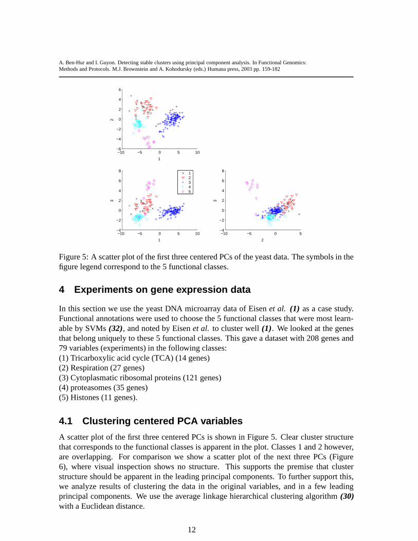
6 Conclusions

In this chapter we propose a novel methodology for evaluating the merit of clustering so-lutions. It is based on the premise that well defined cluster structure should be stable underperturbation of the data. We introduced notions of stability at the level of a partition, clus-ter, and pattern, that allow us, in particular, to generate stability-annotated dendrograms.Using stability as a figure of merit, along with a measure of cluster refinement, allows us tocompare stable solutions run using different normalizations, similarity measures, clusteringalgorithms, or input features.

We demonstrated this methodology on the task of choosing thenumber of principalcomponents and normalization to be used to cluster a yeast gene expression dataset. Itwas shown that PCA improves the extraction of cluster structure, with respect to stability,refinement, and coincidence with known “ground truth” labels. This means that, in thisdata set, the cluster structure is present in directions of largest variance (or best data recon-struction). Beyond this simple example, our methodology can be used for many “modelselection” problems in clustering, including selecting the clustering algorithm itself, theparameters of the algorithm, the variables and patterns to cluster, the similarity, normaliza-tion or other preprocessing, and the number of clusters. It allows us not only to compareclustering solutions, but also to detect presence or absence of structure in data. In our anal-ysis we used a hierarchical clustering algorithm, but any other clustering algorithm can beused. The versatility and universality of our methodology,combined with its simplicity,may appeal to practitioners in Bioinformatics and other fields. Further work include lay-ing the theoretical foundations of the methodology and further testing of the ideas in otherdomains.

AcknowledgementsThe authors thank Andre Elisseeff and Bronwyn Eisenberg for their helpful comments onthis manuscript.

References

1. Eisen, M., Spellman, P., Brown, P. and Botstein, D. (1998)Cluster analysis and displayof genome-wide expression patterns.Proc. Natl. Acad. Sci USA, 95, 14863–14868.

2. Quackenbush, J. (2001) Computational anaysis of microarray data. Nature ReviewsGenetics, 2, 418–427.

3. Ross, D., Scherf, U., Eisen, M., Perou, C., Rees, C., Spellman, P., Iyer, V., Jeffrey,S., de Rijn, M. V., Waltham, M., Pergamenschikov, A., Lee, J., Lashkari, D., Shalon,D., Myers, T., Weinstein, J., Botstein, D. and Brown, P. (2000) Systematic variation ingene expression patterns in human cancer cell lines.Nature genetics, 24, 227–235.

4. D’haeseleer, P., Liang, S. and Somogyi, R. (2000) Geneticnetwork inference: fromco-expression clustering to reverse engineering.Bioinformatics, 16, 707–726.

20


5. Alon, U., Barkai, N., Notterman, D., Gish, G., Ybarra, S.,Mack, D. and Levine, A. J.(1999) Broad patterns of gene expression revealed by clustering analysis of tumor andnormal colon tissues probed by oligonucleotide arrays.PNAS, 96, 6745–6750.

6. Alizadeh, A.A.et al.(2000) Distinct types of diffuse large B-cell lymphoma identifiedby gene expression profiling.Nature, 403, 503–511.

7. Scherf, U., Ross, D. T., Waltham, M., Smith, L. H., Lee, J. K., Tanabe, L., Kohn,K. W., Reinhold, W. C., Myers, T. G., Andrews, D. T., Scudiero, D. A., Eisen, M. B.,Sausville, E. A., Pommier, Y., Botstein, D., Brown, P. O. andWeinstein, J. N. (2000) Agene expression database for the molecular pharmacology ofcancer.nature genetics,24, 236–244.

8. Getz, G., Levine, E. and Domany, E. (2000) Coupled two-wayclustering analysis ofgene microarray data.Proc. Natl. Acad. Sci USA, 94, 12079–12084.

9. Shamir, R. and Sharan, R. (2001) Algorithmic approaches to clustering gene expres-sion data. in Jiang, T., Smith, T., Xu, Y. and Zhang, M., eds.,Current Topics inComputational Biology, MIT Press.

10. Milligan, G. (1996) Clustering validation: results andimplications for applied analy-sis, inClustering and Classification(Arabie, P., Hubert, L. and Soete, G. D., eds.),World Scientific, River Edge, NJ. 341–374.

11. Tibshirani, R., Walther, G. and Hastie, T. (2001) Estimating the number of clusters ina dataset via the gap statistic.Journal of the Royal Statistical Society B, 63, 411–423.

12. Ben-Hur, A., Elisseeff, A. and Guyon, I. (2002) A stability based method for discov-ering structure in clustered data, inPacific Symposium on Biocomputing(Altman, R.,Dunker, A., Hunter, L., Lauderdale, K. and Klein, T., eds.),World Scientific, 6–17.

13. Levine, E. and Domany, E. (2001) Resampling method for unsupervised estimation ofcluster validity.Neural Computation, 13, 2573–2593.

14. Fridlyand, J. (2001)Resampling methods for variable selection and classification:applications to genomics. Ph.D. thesis, UC Berkeley.

15. Fowlkes, E. and Mallows, C. (1983) A method for comparingtwo hierarchical cluster-ings. Journal of the American Statistical Association, 78, 553–584.

16. Bittner, M., Meltzer, P., Chen, Y., Jiang, Y., Seftor, E., Hendrix, M., Radmacher, M.,Simon, R., Yakhini, Z., Ben-Dor, A., Dougherty, E., Wang, E., Marincola, F., Gooden,C., Lueders, J., Glatfelter, A., Pollock, P., Gillanders, E., Leja, D., Dietrich, K., Berens,C., Alberts, D., Sondak, V., Hayward, N. and Trent, J. (2000)Molecular classificationof cutaneous malignant melanoma by gene expression profiling. Nature, 406, 536–540.

21


17. Yeung, K., Haynor, D. and Ruzzo, W. (2001) Validating clustering for gene expressiondata.Bioinformatics, 17, 309–318.

18. Milligan, G. (1980) An examination of the effect of six types of error perturbation onfifteen clustering algorithms.Psychometrika, 45, 325–342.

19. Yeung, K. and Ruzzo, W. (2001) An empirical study of principal component analysisfor clustering gene expression data.Bioinformatics, 17, 763–774.

20. Jackson, J. (1991)A user’s guide to principal components. John Wiley & Sons.

21. Jolliffe, I. (1986)Principal component analysis. Springer-Verlag.

22. Jolliffe, I. (1972) Discarding variables in principal component analysis I: Artificialdata.Applied Statistics, 21, 160–173.

23. Jolliffe, I. (1972) Discarding variables in principal component analysis II: Real data.Applied Statistics, 21, 160–173.

24. Hastie, T., Tibshirani, R., Eisen, M., Alizadeh, A., Levy, R., Staudt, L., Chan, W.,Botstein, D. and Brown, P. (2000) “gene shaving” as a method for identifying distinctsets of genes with similar expression patterns.Genome Biology, 1, 1–21.

25. Alter, O., Brown, P. and Botstein, D. (2000) Singular value decomposition for genome-wide expression data processing and modeling.Proc. Natl. Acad. Sci USA, 97, 10101–10106.

26. Raychaudhuri, S., Stuart, J. and Altman, R. (2000) Principal components analysis tosummarize microarray experiments: Application to sporulation time series, inPacificSymposium on Biocomputing 5, 452–463.

27. Hilsenbeck, S., Friedrichs, W., Schiff, R., O’Connell,P., Hansen, R., Osborne, C. andFuqua, S. (1999) Statistical analysis of array expression data as applied to the problemof tamoxifen resistance.Journal of the National Cancer Institute, 91, 453–459.

28. Wen, X., Fuhrman, S., Michaels, G., Carr, D., Smith, S., Barker, J. and Somogyi,R. (1998) Large-scale temporal gene expression mapping of central nervous systemdevelopment.Proc. Natl. Acad. Sci USA, 95, 334–339.

29. Milligan, G. and Cooper, M. (1988) A study of variable standardization.Journal ofclassification, 5, 181–204.

30. Jain, A. and Dubes, R. (1988)Algorithms for clustering data. Prentice Hall, Engle-wood Cliffs, NJ.

31. Kaufman, L. and Rousseeuw, P. (1990)Finding groups in data. Wiley Interscience,John Wiley & Sons.

22


32. Brown, M., Grundy, W., Lin, D., Cristianini, N., Sugnet,C., Ares, M. and Haus-sler, D. (2000) Knowledge-based analysis of microarray gene expression data byusing support vector machines.Proc. Natl. Acad. Sci. USA, 97, 262–267. URLhttp://www.cse.ucsc.edu/research/compbio/genex.

33. Ben-Hur, A., Horn, D., Siegelmann, H. and Vapnik, V. (2001) Support vector cluster-ing. Journal of Machine Learning Research, 2, 125–137.

34. Anderberg, M. (1983)Cluster analysis for applications. Academic Press, New York.

23

Detecting Stable Clusters Using Principal Component …asa/pdfs/pcachap.pdfPrincipal Component...

Documents

Transcript of Detecting Stable Clusters Using Principal Component …asa/pdfs/pcachap.pdfPrincipal Component...