Designing a hydraulic actuator for the tyre measurementtowerde Wispelaere, H.N.L.

Published: 01/01/2006

Document VersionPublisher’s PDF, also known as Version of Record (includes final page, issue and volume numbers)

Please check the document version of this publication:

• A submitted manuscript is the author's version of the article upon submission and before peer-review. There can be important differencesbetween the submitted version and the official published version of record. People interested in the research are advised to contact theauthor for the final version of the publication, or visit the DOI to the publisher's website.• The final author version and the galley proof are versions of the publication after peer review.• The final published version features the final layout of the paper including the volume, issue and page numbers.

Link to publication

General rightsCopyright and moral rights for the publications made accessible in the public portal are retained by the authors and/or other copyright ownersand it is a condition of accessing publications that users recognise and abide by the legal requirements associated with these rights.

• Users may download and print one copy of any publication from the public portal for the purpose of private study or research. • You may not further distribute the material or use it for any profit-making activity or commercial gain • You may freely distribute the URL identifying the publication in the public portal ?

Take down policyIf you believe that this document breaches copyright please contact us providing details, and we will remove access to the work immediatelyand investigate your claim.

Download date: 12. Jul. 2018

Designing a Hydraulic Actuatorfor the Tyre Measurement Tower

H.N.L. de Wispelaere

DCT 2006.26

Bachelor End Project

Supervisors: dr. ir. A.J.C. Schmeitzdr. ir. W.J.A.M. Post

Technische Universiteit EindhovenDepartment of Mechanical EngineeringDynamics and Control Technology Group

Eindhoven, March, 2006

Abstract

EnglishWhen developing modern control systems like anti-lock braking systems (ABS), traction control (TC),brake assistant (BAS) and electronic stability programs (ESP) to increase safety and comfort in vehi-cles, accurate tyre models are very important. Numerical simulation models are needed to predictthe vehicle’s behaviour for various driving conditions. Testing facilities like the tyre measurementtower are needed to provide the necessary experimental data to validate these tyre models. The tyremeasurement tower of the Dynamics and Control section of the TU Eindhoven, is already capable ofsimulating different situations, but it needs hydraulic actuators to subject the wheel to vertical vibra-tions and alternating steer angles. This report discusses the design of a vertical hydraulic actuatorfor the tyre measurement tower. A theoretical model of the hydraulic actuator and the measurementtower is developed, to determine what size of hydraulic cylinder is needed to fulfill the demands forgood tyre measurement. This is done for a-symmetrical and symmetrical cylinder types. The sizeof these hydraulic cylinders limit the choice between servo valves, and this choice has a substantialeffect on the dynamics of the total system. Some available hydraulic cylinders and servo valves areimplemented in the model, and the performances are analyzed. From this analysis the most suitablehydraulic cylinder and servo valve is determined to complete the measurement tower. Finally, recom-mendations are given on the usage of other hydraulic cylinders, and on additional components thatare required for a functioning hydraulic system.

DutchBij het ontwerpen van moderne regelsystemen zoals "antiblokkeersystemen" (ABS), "wegligging rege-laar" (TC), "rem assistent" (BAS) en "elektronische stabiliteit programma’s" (EPS) voor het verhogenvan de veiligheid en comfort in voertuigen, zijn nauwkeurige autoband modellen heel belangrijk. Nu-merieke simulatiemodellen zijn nodig om het voertuiggedrag voor verschillende rij-situaties te voor-spellen. Test opstellingen zoals de bandenmeettoren zijn nodig om de nodige experimentele data televeren waarop deze modellen gevalideerd kunnen worden. De bandenmeettoren van de sectie ’Dy-namics and Control’ op de TU Eindhoven, kan al verschillende situaties simuleren, maar het ontbreektnog aan hydraulische actuators die het wiel verticaal kunnen laten trillen en de stuurhoek kunnen ve-randeren. Dit verslag bespreekt het ontwerp van een verticale hydraulische actuator voor de banden-meettoren. Een theoretisch model van de hydraulische actuator en de meettoren is ontwikkeld om tebepalen hoe groot een hydraulische cilinder moet zijn die voldoet aan de eisen voor een goede meting.Dit is gedaan voor zowel a-symmetrische als symmetrische cilinder types. De grootte van deze hy-draulische cilinders beperkt de keuze voor een servo klep, en deze keuze heeft een substantieel effectop de dynamica van het gehele systeem. Verschillende beschikbare cilinders zijn geïmplementeerdin het model, en de prestaties zijn geanalyseerd. Uit deze analyse is de meest geschikte hydraulischecilinder en servo klep bepaald om de bandenmeettoren mee te vervolledigen. Uiteindelijk wordener nog aanbevelingen gegeven over het toepassen van andere hydraulische cilinders, en over welkebijkomende componenten nog nodig zijn voor een functionerend hydraulisch systeem.

Contents

List of symbols ii

1 Introduction 11.1 Background . . . . . . . . . . . . . . . . . . . . . . . . . . . . . . . . . . . . . . . . . . 11.2 Aim of this report . . . . . . . . . . . . . . . . . . . . . . . . . . . . . . . . . . . . . . 21.3 Overview . . . . . . . . . . . . . . . . . . . . . . . . . . . . . . . . . . . . . . . . . . . 2

2 Modelling 32.1 The measurement tower . . . . . . . . . . . . . . . . . . . . . . . . . . . . . . . . . . . 32.2 The actuating system . . . . . . . . . . . . . . . . . . . . . . . . . . . . . . . . . . . . . 32.3 The hydraulic model . . . . . . . . . . . . . . . . . . . . . . . . . . . . . . . . . . . . . 52.4 Model of the system in SIMULINK . . . . . . . . . . . . . . . . . . . . . . . . . . . . . 6

3 Design Of The Actuating System 83.1 Demands on the hydraulic actuator . . . . . . . . . . . . . . . . . . . . . . . . . . . . . 83.2 Design of a hydraulic actuator . . . . . . . . . . . . . . . . . . . . . . . . . . . . . . . . 83.3 Increasing bandwidth . . . . . . . . . . . . . . . . . . . . . . . . . . . . . . . . . . . . 113.4 Results of simulations . . . . . . . . . . . . . . . . . . . . . . . . . . . . . . . . . . . . 12

4 Model Validation 14

5 Simulating Servo Systems 165.1 Including the servo valve in the model . . . . . . . . . . . . . . . . . . . . . . . . . . . 165.2 Available cylinders . . . . . . . . . . . . . . . . . . . . . . . . . . . . . . . . . . . . . . 175.3 Options . . . . . . . . . . . . . . . . . . . . . . . . . . . . . . . . . . . . . . . . . . . . 18

5.3.1 A-symmetrical hydraulic cylinder . . . . . . . . . . . . . . . . . . . . . . . . . . 185.3.2 Symmetrical cylinder MTS model 248.02 . . . . . . . . . . . . . . . . . . . . . 195.3.3 Symmetrical cylinder MTS model 248.01 . . . . . . . . . . . . . . . . . . . . . 20

6 Conclusion And Recommendations 21

Appendices 23

A A-symmetric Versus Symmetric Cylinders 23

B Equations 25

C SIMULINK Model 28

Bibliography 29Enclosed: A CD-rom with MATLAB programs

i

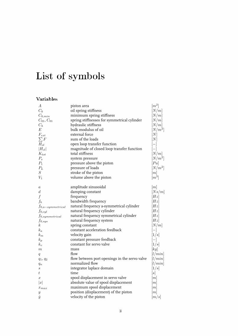
List of symbols

VariablesA piston area [m2]C0 oil spring stiffness [N/m]C0,min minimum spring stiffness [N/m]C01, C01 spring stiffnesses for symmetrical cylinder [N/m]Ch hydraulic stiffness [N/m]E bulk modulus of oil [N/m2]Fext external force [N ]∑

F sum of the loads [N ]Hol open loop transfer function [−]|Hcl| magnitude of closed loop transfer function [−]Ktot total stiffness [N/m]Ps system pressure [N/m2]P1 pressure above the piston [Pa]PL pressure of loads [N/m2]S stroke of the piston [m]V1 volume above the piston [m3]

a amplitude sinusoidal [m]d damping constant [Ns/m]f frequency [Hz]fb bandwidth frequency [Hz]f0,a−symmetrical natural frequency a-symmetrical cylinder [Hz]f0,cyl natural frequency cylinder [Hz]f0,symmetrical natural frequency symmetrical cylinder [Hz]f0,sys natural frequency system [Hz]k spring constant [N/m]ka constant acceleration feedback [−]km velocity gain [1/s]kp constant pressure feedback [−]kv constant for servo valve [1/s]m mass [kg]q flow [l/min]q1, q2 flow between port openings in the servo valve [l/min]qn normalized flow [l/min]s integrator laplace domain [1/s]t time [s]x spool displacement in servo valve [m]|x| absolute value of spool displacement [m]xmax maximum spool displacement [m]y position (displacement) of the piston [m]y velocity of the piston [m/s]

ii

β damping in the cylinder [−]ω0,a−symmetrical natural frequency a-symmetrical cylinder [rad/s]ω0,cyl natural frequency cylinder [rad/s]ω0,symmetrical natural frequency symmetrical cylinder [rad/s]ω0,sys natural frequency system [rad/s]

iii

Chapter 1

Introduction

1.1 BackgroundIn the world of tyre, wheel and automotive industries testing equipment is very important when de-signing a new and better product. Almost every vehicle manufacturer uses the "Magic Formula", a tyremodel developed by Professor Hans Pacejka, in their vehicle dynamics simulations. This tyre modelis the subject of continuous development. When developing modern control systems like anti-lockbraking systems (ABS), traction control (TC), brake assistant (BAS) and electronic stability programs(ESP) to increase safety and comfort, tyre modelling is crucial [1].

The research field of vehicle dynamics, of the Dynamics and Control section of the TU/e, is stronglyfocused on the development of simulation models to predict vehicle behaviour for various driving con-ditions (e.g. different road surfaces). In the Automotive Laboratory, testing facilities are available forexperimental research to validate these numerical simulation models. In this report the measurementtower is discussed, which is an experimental setup of the Dynamics and Control section of the TUEindhoven (figure 1.1).

The measurement tower consists of a construction on which the wheel carrier is mounted. The wheelis in contact with a large drum (3) that drives the wheel at different speeds.

View fromabove

1

wheel

Frontview

3

4

Hydraulicactuator

Side-view

drum

2fork

5

Figure 1.1: The measurement tower with a hydraulic actuator [2]

1

The measurement tower is able to simulate a few different situations: the steer angle (1) can be altered,and the drum (3) can drive the wheel (4) at different speeds. Experimental setups like the measure-ment tower at the TU/e mostly include a few hydraulic actuators. With hydraulic actuators, the wheelcan easily be subjected to (dynamic) displacements (2) and (alternating) steer angles (1). Adding thesehydraulic actuators makes it possible to determine the dynamic response of a tyre.

1.2 Aim of this reportThe aim of this report is to complete the measurement tower with a hydraulic actuator. With a hy-draulic actuator, the measurement tower will be able to measure the dynamic response of differentkind of tyres. This hydraulic actuator (see figure 1.1) must be capable of delivering dynamic loads onthe wheel. In this report, only a vertical actuator is considered.

The first goal of this report is to design a hydraulic actuator that fulfills the demands for good tyremeasurement. Some of these demands are given in an earlier report [2], and some new demands areadded. From a developed model, the size of the cylinder can be determined. This is done for botha-symmetrical and symmetrical cylinders. The size of these hydraulic cylinders limit the choice onservo valves. From the size of the cylinders the needed flow is determined, which is a guideline fordetermining the servo type of valve.

Secondly, the data of available hydraulic cylinders and servo valves is implemented in the model.The results on the dynamic response are discussed for different types of servo valves and hydrauliccylinders. From this analysis, the most suitable hydraulic cylinder and servo valve is determined forthe measurement tower.

1.3 OverviewThis report consists of two parts. The first part deals with modelling and designing a hydraulic actua-tor with the right size. First a model of the hydraulic cylinder with measurement tower is developed inchapter 2. This physical model will be implemented in SIMULINK, to be able to simulate and developthe hydraulic actuator.

In chapter 3, the model of the hydraulic actuator is adapted to meet the design demands. A controlleris designed and some considerations are presented to increase the bandwidth of the system. Aftertuning the system, the size of the theoretically developed hydraulic actuator is known.

To validate the developed model, the simulated transfer functions from the SIMULINK program arecompared with measurements on an existing hydraulic actuator in chapter 4.

The second part, chapter 5, deals with available hydraulic cylinders and servo valves. These cylindersand servo valves are simulated, and the results are analyzed.

Finally, chapter 6 concludes which of the hydraulic cylinders and servo valves are most suitable for themeasurement tower. Further, some recommendations are given.

2

Chapter 2

Modelling

In this first chapter the measurement tower and the hydraulic actuator will be analyzed. The model ofthe measurement tower is known from an earlier report [2], and so are some of the demands for thehydraulic actuator. The purpose of this chapter is to develop a method for determining the size of thehydraulic cylinder so that it meets the demands set in the earlier report. Therefore, the measurementtower and the hydraulic actuator are modelled in MATLAB and SIMULINK.

2.1 The measurement towerAs mentioned earlier, the model of the measurement tower is already known and so are the values ofthe variables. The model is represented by a mass-spring-damper system shown in fig 2.1, where mrepresents the total mass of the wheel carrier, rim and tire. The constants k and d are typical stiffnessand damping values for a passenger car tyre.

y

k d

m

m kgd Ns/m

k N/m

= 250 [ ]

= 250 [ ]

= 200 [ ]·103

Figure 2.1: Model of the measurement tower

2.2 The actuating systemThe hydraulic actuator will first be modelled as a cylinder with a flow supply delivered by an ideal servovalve. After analyzing the model and the outcoming results, the servo type of valve that is needed tofulfill the required demands on pressure and flow can be determined. This will be done in chapter 5.

First the a-symmetrical cylinder will be discussed. This cylinder consists of a rod that is attached to thepiston. This rod connects the piston with a mechanical system, in this case the mass-spring-dampersystem of the measurement tower (see figure 2.2). The piston, connecting rod and mass of the mea-surement tower are modelled as a rigid body with a total mass m. Note that this changes the definition

3

of the total mass m presented in the previous paragraph.

Consequently, the displacement y of the mass m in figure 2.1 now equals the position of the rod ofthe cylinder which is positive defined downwards. To realize a positive piston displacement, the servovalve should be able to deliver a positive flow q to the hydraulic cylinder. In figure 2.2, the hydrauliccylinder is controlled by a valve. The spool displacement x in this valve, changes the port opening thatresults in a change in the flow q from servo valve to hydraulic cylinder. This flow results in a positiveor negative piston motion. Part of the flow q is also needed to compensate for the leakages that arepresent in the cylinder.

A2

1

A

SP

SP

1P

x

q

y

k d

m

0C

Figure 2.2: A-symmetrical cylinder connected to the measurement tower

In the hydraulic cylinder shown above there are a few properties that are of interest for modelling. Anideal servo valve is assumed, meaning that the valve has no dynamics and it completely controls themotion of the piston. When the flow q exceeds the compensation flow needed for leakages, the pistonwill be forced to move downwards (y > 0). This creates an oil volume (column) above the piston witha certain stiffness C0 (see equation 2.1 and figure 2.2). This (column) stiffness depends on the strokey, piston area A and the bulk modulus of oil E, and can be modelled as a spring between the pistonand cylinder end.

C0 =AE

y(2.1)

This (spring) stiffness C0 in the a-symmetrical cylinder is in parallel to the spring k of the tyre in themeasurement tower. The model can be simplified by combining these springs:

Ktot = C0 + k (2.2)The spring stiffness in the hydraulic actuator can now be replaced with the total stiffness Ktot. Thedamper d in the measurement tower model can be included in the external force Fext, which alreadycontains the gravity force, see figure 2.3:

Fext = mg − dy (2.3)Replacing the stiffness in the hydraulic actuator with the total stiffness Ktot and including the damperd in the external force Fext reduces the model of figure 2.2 to the model of figure 2.3. Here it is chosen

4

to integrate the spring and damper of the measurement tower in the model of the hydraulic cylinder.This reduced model approaches the theoretical models in the applied literature of the course HydraulicServo Systems [3], what simplifies the determination of the equations needed to describe this model.

A2

1

A

SP

SP

1P

x

q

y

m

totK

extF

Figure 2.3: Reduced model of a-symmetrical cylinder on measurement tower

2.3 The hydraulic modelTo find the equations needed for designing the hydraulic actuator, the hydraulic model must be furtherexamined. The valve will still be regarded ideal and the pressure supply will be assumed constant. Inchapter 5, the effect of available valves shall be introduced, analyzed and modelled. For the purpose ofbetter understanding, the derivation of equation 2.4 is given in appendix B. Equation 2.4 applies to ana-symmetrical cylinder controlled by a critical center servo valve, like the one in figure 2.3.

y = km

(x−

∑F

Ch

)−

∑F

C0(2.4)

As in figure 2.2 and equation 2.1, C0 refers to the spring stiffness of fluid inside the a-symmetriccylinder. An equation similar to equation2.4 can be derived for symmetric cylinders (see appendix A).In this equation, x denotes the spool displacement in the servo valve and Ch refers to the hydraulicstiffness of the cylinder. This hydraulic stiffness reacts as a spring (i.e. stiffness) to the mechanicalsystem, but has the unit of damping. The value of the hydraulic stiffness strongly depends on the typeof servo valve that is used (see appendix B). The velocity gain km gives the linear relation betweenthe spool displacement of the valve x and velocity y of the piston. This velocity gain is a constant thatstrongly depends on the valve geometry (see Appendix B). The sum of the forces

∑F in equation

2.4 consists of the external forces acting on the rigid body with mass m in figure 2.3. Gravity and thedamping of the tyre in measurement tower model were already considered external forces in equation2.3, which yields equation 2.5:

∑F = my − Fext = my + dy −mg (2.5)

According to paragraph 2.2, spring stiffness C0 can be replaced by the total spring stiffness Ktot,which includes the spring in the measurement tower model:

y = km

(x−

∑F

Ch

)−

∑F

Ktot(2.6)

5

The model introduced in the previous paragraph is now totally described by equations (2.6) and (2.5).Before implementing this in a MATLAB and SIMULINK program, the model will be further com-pleted to meet our needs.

2.4 Model of the system in SIMULINKBefore the model can be implemented in SIMULINK, equations (2.6) and (2.5) are transferred to theLaplace domain. First, equation 2.6 is rewritten to another form:

∑F

Ktot= km

(x−

∑F

Ch

)− y (2.7)

Transferring (2.7) and (2.5) to the Laplace domain yields:

s∑

F (s)Ktot

= km

(X(s)−

∑F (s)Ch

)− sY (s) (2.8)

∑F (s) = ms2Y (s) + dsY (s)− Fext (2.9)

In equation 2.9, the gravity force mg is now replaced with Fext, because it is independent on thedisplacement of the rigid body y:

∑F (s) = ms2Y (s) + dsY (s)−mg (2.10)

In this form, the equation approximates the one used in literature [3]. After transferring the equationsto the Laplace domain, the model can be put in a block representation 2.4.

hC

1

s

Ktot

extF

X1

s

1

d

mkS

Y+F

--

-

ms

2YY SS

Figure 2.4: Block representation of model in Laplace domain

In figure 2.4, both equations (2.8) and (2.10) can be found starting in the middle of the bock represen-tation, namely with the sum of the forces

∑Fext . The loop right of this unit corresponds to equation

(2.8), and the loop on the left side to equation (2.10).

In general, the hydraulic actuator with measurement tower can also be completely described by theblock representation of figure 2.4. This representation can directly be transferred to a computer pro-gram in SIMULINK.

In figure 2.5, the model in SIMULINK is shown. Clearly, on the right side the block representation offigure 2.4 can be found, including position feedback control. This feedback includes a controller thathas to be designed and a servo valve with no dynamics. As mentioned earlier, the effects of a real servovalve will be determined once the size of the hydraulic cylinder is known (chapter 5). In this modelthe dynamic behaviour will be modelled with only sinusoidal input signals. Note that the gravity force

6

Figure 2.5: The model implemented in SIMULINK (see also appendix C)

is connected to a terminator and not included in the model. The gravity force mg, also denoted asexternal force Fext, is independent of the piston displacement y. This force can be used as a staticload on the tyre, next to a fixed load of the hydraulic actuator. Because the model will only examinedynamic responses, these static (steady-state) loads will be not be included in the model and can beneglected. In the next chapter the model from figure 2.5 will be further adapted to the actual demandson dynamic behaviour.

7

Chapter 3

Design Of The Actuating System

In this chapter, the model of the hydraulic actuator and measurement tower will be adapted to thedemands of the hydraulic actuator. From the earlier HTS graduation report [2], the demands are knownon which the hydraulic actuator will be sized. First these demands will be recalled and updated, andthen the system will be optimized for this situation. After analyzing the results, the sizes of thedifferent types of hydraulic cylinders are known.

3.1 Demands on the hydraulic actuatorThe demands, in the earlier HTS graduation report referred to as ’wishes’, are shown in table 3.1. Forthis report, some of the demands on the hydraulic actuator were altered. These new demands aredepicted next to the demands of the HTS-report.

Demands HTS-report New DemandsMaximum static force [N] 9000 9000Stroke [mm] 160 160Sinusoid frequency [Hz] 8 20Sinusoid amplitude [mm] 20 10

Table 3.1: Demands on the hydraulic actuator

The demands on maximum force and stroke are restraints on the measurement tower itself. The staticforce of the actuator may not exceed 9 kN, because when it reaches 10 kN the measuring instrumenton the wheel will be damaged. In the HTS-report a limit of 9 kN is chosen, including a safety factor.The stroke is limited too, because the maximum displacement of the wheel carrier in the measurementtower is restricted to 160 mm. The last two demands are variable, and only here the demands ofthe HTS-report differ from the new demands on the behaviour of the hydraulic actuator. The newdemands, on which the size of the vertical hydraulic actuator will be designed, require an increasedsinusoidal frequency and have a reduced demand on amplitude. Now the demands are known, thesize of the hydraulic actuator can be determined.

3.2 Design of a hydraulic actuatorNow the system parameters are known and the demands are set, the model can be further developedto determine the size of the hydraulic cylinder. A way to start is to determine the minimum naturalfrequency needed to perform under the severest demands. From the natural frequency, the piston

8

area of the cylinder can be calculated. Equation 3.1 applies to a-symmetrical cylinders, but the designprocess of symmetrical cylinders is similar (see appendix A).

ω0,cyl =

√C0,min

m=

√AE

mS(3.1)

In this equation, C0,min denotes the minimum oil spring stiffness and S refers to the stroke (incontrast with equation 2.1, where the displacement y was considered). To determine the minimumnatural frequency of the cylinder ω0,cyl, equation 3.1 must be used. The natural frequency, and oilstiffness, strongly depend on the displacement of the piston in the hydraulic cylinder. The othervariables in the right part of equation 3.1 are known and assumed constant. The dimension of thehydraulic cylinder will be determined on basis of the minimum natural frequency, and thus on thestroke S (see appendix A). In this report f0 and ω0 both refer to natural frequency (see list of symbols),using equation 3.2:

f0 =ω0

2π(3.2)

First a natural frequency will be selected, to be able to implement the model in the simulation pro-gram MATLAB. From this natural frequency, other system parameters (e.g. the piston area A) can bedetermined. Note that in (3.1), only the spring stiffness of the cylinder C0,min is used and not the totalstiffness Ktot mentioned in paragraph 2.2. The spring stiffness of the cylinder is variable, and so isthe natural frequency of the hydraulic cylinder . Now only the hydraulic cylinder is considered, andnot the total system that includes the measurement tower. To calculate the natural frequency of thetotal system, the spring stiffness C0,min should be replaced by the total spring stiffness Ktot.

There is a standard routine to determine if the natural frequency is chosen right, i.e. meets the de-mands on frequency and amplitude. First a value for natural frequency must be chosen or guessed.This natural frequency limits the bandwidth of the closed loop feedback system. So, if the naturalfrequency is high enough, the system will follow the input frequency on phase and amplitude closely,otherwise the output signal will have a phase delay and amplitude decrease.

In general, the bandwidth fb is defined to be the maximum frequency at which the output of the sys-tem will track an input sinusoid in satisfactory manner. In this report, the bandwidth is defined to bethe frequency where the sinusoidal input signal r on the control system is attenuated to the output y.In a Bode diagram, this refers to the frequency where an open loop transfer function intersects withthe 0 dB line in the magnitude plot.

First the transfer function must be determined, before something can be stated about the bandwidthof the system. Equation 3.3 shows the general open loop transfer function of a hydraulic actuator. Thisequation can be derived from the standard equation 2.4 (see appendix B). In this equation, kv is aconstant that equals the velocity gain km, when assuming an ideal servo valve. β denotes the dampingof the system, and a realistic values can be found in the literature [3].

Hol =kv

s(

s2

ω20,cyl

+ s 2βω0,cyl

+ 1) (3.3)

Now, a good estimate can be made on how the hydraulic system will react on different input frequen-cies. When a realistic value for damping (β = 0.1) is chosen and an ideal servo valve (kv = km = 1)is assumed, the transfer function can be calculated. If the natural frequency of the hydraulic servocylinder is chosen to be 20 Hz, MATLAB returns the magnitude plot of figure 3.1.

Note that the transfer functions in figure 3.1 show a −1 slope for frequencies lower than the naturalfrequency, and a −3 slope for frequencies higher than the natural frequency. The −1 slope comesfrom the hydraulic cylinder, where the spool displacement x in the servo valve yields the needed flow

9

100

101

102

−100

−80

−60

−40

−20

0

20

40

frequency [Hz]

mag

nitu

de [d

B]

transfer function of hydraulic cylinder, theoretical

H open loopCH open loop with C=p

Figure 3.1: A-symmetric hydraulic cylinder with f0 = 20 [Hz].

to move the piston in the hydraulic cylinder. The actuator’s behaviour on low frequencies is consid-ered to be an integrator (see appendix B). The other physical properties of a hydraulic cylinder resultin a second order system, which is in series with the integrator. A second order system has a typical−2 slope in a frequency response diagram. Because these systems are in series, the −3 correspondsto the total of the first and second order system. This can also be derived from the transfer function ofa hydraulic cylinder with servo valve, presented in equation 3.3.

In figure 3.1, the lowest graph refers to the open loop transfer function with no controller. For thistransfer function of the a-symmetrical cylinder, also described by equation 3.3, a controller can be de-signed.

For reasons of stability, there is a simple guideline that restricts the gain of a proportional controller:the top of the resonance peak should be 5 dB under the zero dB line. This follows from the stabilitycriterion for the magnitude of the closed loop transfer function |Hcl| = m = 1.3 in a Nyquist diagram,stated in literature [3]. This makes that the open loop characteristic in figure 3.1 can be increased ingain, which results in a larger bandwidth of the system. The open loop transfer function with con-troller has a bandwidth of approximately 2.2 Hz.

Because this example above does not meet the demands, the natural frequency has to be increased.For this a-symmetric cylinder, an sinusoid input signal r with a frequency of 20 Hz would be attenu-ated to the output y with a factor of 0.56.

Note that in case of a symmetric cylinder, the design process is identical but with different values forthe surface area of the piston A and the minimum (spring) stiffness C0,min (see appendix A).

10

3.3 Increasing bandwidthA possible solution to increase the bandwidth of the system is choosing a larger cylinder, with a largerpiston area, which results in a higher natural frequency (see equation 3.1). From the previous para-graph can be concluded that the natural frequency of the cylinder should be at least well above thementioned 20 Hz, to create a bandwidth of 20 Hz. Increasing the natural frequency automaticallyleads to a larger cylinder.

Another way to increase the bandwidth is making use of pressure or acceleration feedback. Both thepressure and the acceleration feedback will give the same outcome by increasing the damping of thehydraulic cylinder, which reduces the resonance peak at the natural frequency. In case of accelerationfeedback, the piston acceleration in the hydraulic cylinder is measured by a transducer. The outputof this signal is used as a feedback signal on the spool displacement x of the servo valve (see figure 3.2).

mks

K totvalvecontrollerm

1

s

1

s

1

d

pk

akOption 1: Acceleration Feedback

Option 2: Pressure Feedback

r e 2sY sY Y

F

hC

1

---

- -

S

Figure 3.2: Pressure and acceleration feedback.

An alternative for measuring acceleration is using a pressure transducer which is mounted on thestanding cylinder. The pressure inside the cylinder is measured, and the output of the transducer isagain used as feedback on the spool displacement x of the servo valve.

Figure 3.3 shows a Bode diagram of two closed loop transfer functions. First, the closed loop transferfunction of hydraulic cylinder is plotted with a natural frequency of 40 Hz (upper graph). The onlydifference with figure 3.1 is the choice of a larger hydraulic cylinder. The proportional controller isdesigned, according to the guideline in the previous paragraph, on a magnitude of -5 dB at the naturalfrequency of the open loop transfer function for reasons of stability.

Secondly, the transfer function of the system is shown with pressure feedback, as modelled in theblock diagram of figure 3.2. The transfer function of this system is determined by putting a whitenoise signal on the input of the system, and then measuring the output.

For the considered pressure or acceleration feedback, the constants ka and kp should be determinedby trial and error. The intended result is to increase damping and reducing the resonance peak, asfigure 3.3 shows. From the phase plot can be seen that the phase has shifted 180 degrees at the naturalfrequency. This is in accordance with the literature, but is of minor importance when developing avertical hydraulic actuator for the measurement tower.

Now the pressure feedback is applied and the resonance peak is damped, the proportional controller

11

10−1

100

101

102

−60

−40

−20

0

20

40Transfer function closed loop r−>y

Frequency [Hz]

Mag

nitu

de [d

B]

TF of system with pressure feedbackTF of hydraulic cylinder

10−1

100

101

102

−350

−300

−250

−200

−150

−100

−50

0

Frequency [Hz]

Pha

se [d

eg]

TF of system with pressure feedbackTF of hydraulic cylinder

Figure 3.3: Transfer function closed loop with and without pressure feedback.

can be tuned to increase the bandwidth of the system (see figure 3.4). In the literature [3] is also men-tioned how far the gain of the p-action can be increased before the system becomes unstable. Thecontroller has to be tuned by taking into account the resonance peak in the Bode diagram. Whenthe controller is tuned too high, the system will be on the edge of stability. On the other hand, if thecontroller is tuned too weak the performance of the system will be poor for its size and costs.

The system in its current form, including pressure feedback and completely tuned, has a bandwidthat about 23 Hz. On that frequency the system shows a phase shift of 108 degrees. This means thata sinusoidal input signal with frequency of 23 Hz, would not attenuate the system’s output signal onamplitude and would have a phase shift of 108 degrees.

The hydraulic actuator is only designed on the magnitude response, because phase response is notrelevant for this application. Most importantly should the actuator be able to put a sinusoidal signal(with frequencies up to 20 Hz) on the measurement tower. This is a constant signal, where a phaseshift between the input signal r and output signal y is of minor importance as long as the system staysstable.

3.4 Results of simulationsIn the previous paragraph a hydraulic actuator is developed on the demands of table 3.1. Note thatthe hydraulic cylinder is designed on natural frequency, and that this does not affect the choice of asymmetric or a-symmetric cylinder. If a symmetric and a-symmetric cylinder have a equal naturalfrequency, they will have a different size due to the different piston area.

The natural frequency of both types of hydraulic systems is designed on a frequency of 40 Hz. Withequation 3.1, the minimum spring stiffness and piston area for an a-symmetrical can be calculated:C0,min = 15, 8 · 106 [N/m] and Aa−sym = 2567 [mm2].The symmetrical cylinder has a equal spring stiffness: C0,min,a−sym = 15, 8 · 106 [N/m], and the

12

10−1

100

101

102

−60

−40

−20

0

20

40Transfer function closed loop r−>y

Frequency [Hz]

Mag

nitu

de [d

B]

TF of system with pressure feedbackTF of hydraulic cylinder

10−1

100

101

102

−350

−300

−250

−200

−150

−100

−50

0

Frequency [Hz]

Pha

se [d

eg]

TF of system with pressure feedbackTF of hydraulic cylinder

Figure 3.4: Transfer function of tuned system with pressure feedback.

piston area can be calculated with equation A.6: Asym = 631, 6 [mm2].

More precisely, the piston area of an a-symmetrical cylinder has to be four times larger than that of asymmetrical cylinder. This can be easily derived from appendix A. In general, a symmetrical type ofcylinder is preferred above an a-symmetrical, but this also shows in price difference between the two.

These hydraulic cylinders are designed on a natural frequency of 40 Hz, and in accordance withequation 3.1 the spring stiffness is calculated. As mentioned, the total spring stiffness Ktot of thesystem does not only consist of the spring stiffness of the cylinder C0,min , but also of a spring k fromthe tyre in the measurement tower. This means that the natural frequency of the system ω0,sys issomewhat higher than the natural frequency of the cylinder ω0,sys.

ω0,sys =

√Ktot

m=

√C0,min + k

m(3.4)

Summing both stiffnesses yields the total stiffness of the system (Ktot =16 · 106 [N/m]) which is notso much different from the cylinder’s spring stiffness, because the spring in the measurement toweris very small compared with the oil’s spring stiffness. According to equation 3.4, the system’s naturalfrequency can be calculated and yields f0,sys = 40,25 [Hz].

Note that this also applies to figures 3.3 and 3.4, where the plot with resonance peak refers to the hy-draulic cylinder and the other to the whole system. Because of the little difference, this does not affectthe results on size for the designed cylinder.

13

Chapter 4

Model Validation

The general approach that was chosen to model the hydraulic actuator is based on theory presented inappendix B. To verify that the equations and assumption in this approach are valid, the model will becompared with measurements executed on a hydraulic actuator system.The measurements were executed on an a-symmetrical cylinder that was connected to a load with amass of 130 kg. The piston was positioned on a stationary position y, to be able to consider a constantnatural frequency. The input signal r working on the spool displacement in the servo valve was asinusoidal with low frequency and amplitude. A random noise signal with a frequency contents upto 200 Hz was used to actuate the system, while the system was controlled by a weak proportionalcontroller to keep the cilinder in the desired position.

Figure 4.1 shows the measured frequency response of this hydraulic cylinder with servo valve. Here,the piston was positioned on half of cilinder’s stroke, which corresponds to a position of y = 100[mm]. The characteristic data of this hydraulic cylinder was inserted into the theoretical model, whichyields the simulated frequency response.

100

101

102

−60

−50

−40

−30

−20

−10

0

frequency [Hz]

100

101

102

−200

−100

0

100

200

frequency [Hz]

Measured Simulated

Figure 4.1: Simulated and measured transfer function open loop, y = 100 [mm]

First, and most importantly, it can be noticed that the natural frequencies in this figure are equal;f0 = 62 [Hz]. Secondly, both transfer functions show a −1 slope in the frequency range under thenatural frequency, and a−3 slope at higher frequencies than the natural frequency, in accordance withthe explanation on page 10.

14

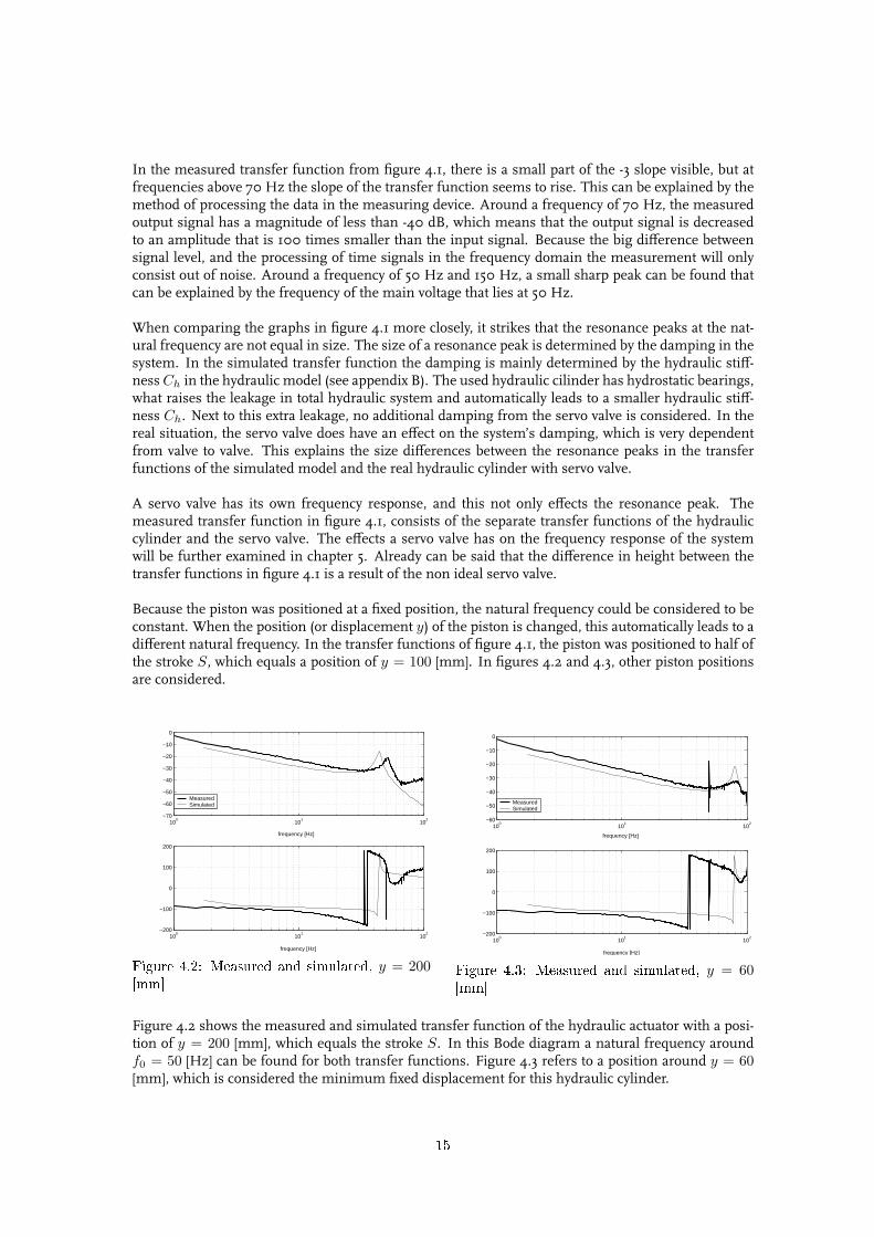
In the measured transfer function from figure 4.1, there is a small part of the -3 slope visible, but atfrequencies above 70 Hz the slope of the transfer function seems to rise. This can be explained by themethod of processing the data in the measuring device. Around a frequency of 70 Hz, the measuredoutput signal has a magnitude of less than -40 dB, which means that the output signal is decreasedto an amplitude that is 100 times smaller than the input signal. Because the big difference betweensignal level, and the processing of time signals in the frequency domain the measurement will onlyconsist out of noise. Around a frequency of 50 Hz and 150 Hz, a small sharp peak can be found thatcan be explained by the frequency of the main voltage that lies at 50 Hz.

When comparing the graphs in figure 4.1 more closely, it strikes that the resonance peaks at the nat-ural frequency are not equal in size. The size of a resonance peak is determined by the damping in thesystem. In the simulated transfer function the damping is mainly determined by the hydraulic stiff-ness Ch in the hydraulic model (see appendix B). The used hydraulic cilinder has hydrostatic bearings,what raises the leakage in total hydraulic system and automatically leads to a smaller hydraulic stiff-ness Ch. Next to this extra leakage, no additional damping from the servo valve is considered. In thereal situation, the servo valve does have an effect on the system’s damping, which is very dependentfrom valve to valve. This explains the size differences between the resonance peaks in the transferfunctions of the simulated model and the real hydraulic cylinder with servo valve.

A servo valve has its own frequency response, and this not only effects the resonance peak. Themeasured transfer function in figure 4.1, consists of the separate transfer functions of the hydrauliccylinder and the servo valve. The effects a servo valve has on the frequency response of the systemwill be further examined in chapter 5. Already can be said that the difference in height between thetransfer functions in figure 4.1 is a result of the non ideal servo valve.

Because the piston was positioned at a fixed position, the natural frequency could be considered to beconstant. When the position (or displacement y) of the piston is changed, this automatically leads to adifferent natural frequency. In the transfer functions of figure 4.1, the piston was positioned to half ofthe stroke S, which equals a position of y = 100 [mm]. In figures 4.2 and 4.3, other piston positionsare considered.

100

101

102

−70

−60

−50

−40

−30

−20

−10

0

frequency [Hz]

100

101

102

−200

−100

0

100

200

frequency [Hz]

MeasuredSimulated

Figure 4.2: Measured and simulated, y = 200[mm]

100

101

102

−60

−50

−40

−30

−20

−10

0

frequency [Hz]

MeasuredSimulated

100

101

102

−200

−100

0

100

200

frequency [Hz]

Figure 4.3: Measured and simulated, y = 60[mm]

Figure 4.2 shows the measured and simulated transfer function of the hydraulic actuator with a posi-tion of y = 200 [mm], which equals the stroke S. In this Bode diagram a natural frequency aroundf0 = 50 [Hz] can be found for both transfer functions. Figure 4.3 refers to a position around y = 60[mm], which is considered the minimum fixed displacement for this hydraulic cylinder.

15

Chapter 5

Simulating Servo Systems

In the previous part of the report, the aim was to design a hydraulic cylinder on basis of the givendemands. Now that the sizes of the developed symmetrical and a-symmetrical cylinders are known,the model can be extended. Out of the size of the hydraulic cylinders, the needed flow and pressurecan be determined and a servo valve can be chosen and implemented in the model. The dynamics ofa servo valve model may be approximated by a second order approximation of the frequency responsedata from available servo valves. In combination with these servo valves, some available hydrauliccylinders will be implemented and analyzed.

5.1 Including the servo valve in the modelSo far, the servo valve in our model was assumed ideal. To be able to assume that a servo valve actsideal, the natural frequency of the servo valve should be about twice as high as the natural frequencyof the hydraulic system (see course Hydraulic Servo Systems [3]). Although this assumption is a goodapproximation of reality, in this chapter the servo valve will assumed non ideal.The sizes of the developed hydraulic cylinder types are determined in paragraph 3.4. From the sizesand the demands on frequency and amplitude from table (3.1), the flow q can be determined. First themaximum velocity of the piston is determined.

Assume that the piston’s motion follows a harmonic input signal, described by equation 5.1:

y = a · sin(2πft) (5.1)y describes the piston displacement, f the frequency of sinusoidal signal and a, t respectively relateto sinusoid amplitude and time. The velocity of the piston y can be obtained by differentiating thisfunction:

y = −2πf · a · cos(2πft) (5.2)Hence, the maximum velocity:

vmax = 2πf · a (5.3)Assuming a sinusoidal signal with frequency of f = 20 [Hz] and amplitude of a = 10 [mm], yieldsa maximum velocity of vmax = 1.26 [m/s]. From this maximum velocity, the maximum flow can bedetermined:

q = vmax ·A (5.4)The flow demand for the theoretical determined a-symmetrical and symmetrical cylinders are givenin table 5.1.

16

Piston area A[mm2]

Flow q[l/min]

a-symmetrical cylinder 2567 194symmetrical cylinder 632 48.6

Table 5.1: Theoretical �ow demands for servo valves

The servo valve model will be approximated with data from available servo valves to describe its dy-namic behaviour. This data consist of a frequency response and is plotted in a Bode diagram. Thisdata is fitted with a second order approximation in a MATLAB program, see figure 5.1. The data inthis figure refers to a standard two stage servo valve (Moog model 76-104) with a pressure range of 15to 210 bar, and can deliver a nominal flow of q = 57 [l/min] at ∆P = 70 [bar].

This flow restricts the choice between the cylinder types in table 5.1. Only the symmetrical cylinderhas a flow requirement that can be provided by this servo valve. Figure 5.2 shows the transfer functionof the developed hydraulic actuator with this servo valve. Also depicted in this figure is the transferfunction of the hydraulic actuator with an ideal assumed servo valve. It is shown that this servo valvedoes have its influences on the frequency response of the hydraulic actuator. Although this modelincludes pressure feedback, determined according to the method used in paragraph 3.3, two naturalfrequencies can be found. These refer to the natural frequencies of the hydraulic system and the servovalve. Implementing a real servo valve also changes the damping of the system, which means that thecontroller has to be tuned for this specific situation.

101

102

−20

−15

−10

−5

0

frequency [Hz]

mag

nitu

de [d

B]

data servo valve2nd order approximation

101

102

−200

−150

−100

−50

0

frequency [Hz]

phas

e [d

eg.]

Figure 5.1: Servo valve approximation

10−1

100

101

102

−80

−60

−40

−20

0

20

frequency [Hz]

mag

nitu

de [d

B]

10−1

100

101

102

−500

−400

−300

−200

−100

0

frequency [Hz]

phas

e [d

egre

es]

ideal servo valvenon ideal servo valve

Figure 5.2: Model with non ideal servo valve

Already can be concluded that the developed symmetrical cylinder combined with this servo valvecomplies with the requirements on which the system was designed. According to the definition onpage 9, a bandwidth of fb = 22 [Hz] can be found in figure 5.2. Note that the transfer function in themagnitude plot of the Bode diagram rises above the 0 dB line around a frequency of 15 Hz. This meansthat the system’s input sinusoid signal is amplified around this frequency. This dynamic behaviourcan be adjusted by reducing the p-action of the controller, or expanding the model with e.g. a notchfilter.

5.2 Available cylindersNow that the model of the hydraulic actuator is expanded with a non ideal servo valve, some differentsituations can be regarded. In this paragraph, the sizes of available cylinders will be implemented in

17

the model in combination with available servo valve data.In table 5.2 the sizes of a few available hydraulic cylinders are given. The measurement cylinder wasused to validate the model in chapter 4, and the other cylinders are part of the Series 248 HydraulicActuators from MTS Systems Corporation.The piston area A is denoted for each cylinder and with equation 5.4 the flow q is determined. Fromthe piston area of these hydraulic cylinders, the natural frequency ω0 can be determined with equation2.1 (or equation A.6 for symmetrical cylinders). In the equations for the natural frequency, the massm and position y are assumed to be equal to the constants used in the model of the hydraulic actuatorand measurement tower in figure 2.3).

Piston areaA [mm2]

Flow q[l/min]

Natural frequencyf0 [Hz]

Measurement cylinder (a-sym) 1900 143 35MTS model 248.01 (sym) 523 39,4 36MTS model 248.02 (sym) 832 62,7 46MTS model 248.03 (sym) 1452 110 61

Table 5.2: Available cylinders

In table 5.2, the MTS models 248.01 and 248.02 seem to be the most applicable hydraulic cylindersto use for the measurement tower. This can be concluded out of the natural frequencies and the re-quired flow. Like in the theoretical developed hydraulic actuator, natural frequencies around 40 Hzare needed to meet the demands from table 3.1.

The maximum required flows q, denoted in table 5.2, that these hydraulic cylinders need to perform inthe most extreme circumstances are needed to choose the appropriate servo valve. Standard two stageservo valves, like the one in figure 5.1, are capable of delivering flows up to 65 l/min. When flows above65 l/min are required, other types of servo valves, e.g. three stage servo valves, must be considered.Three stage servo valves can deliver more flow to the cylinder but have lower natural frequencies. Thismeans that their dynamic behaviour is worse than that of a two stage servo valve. Three stage servovalves deliver more flow, but the spool size restricts their motion dynamics. In this report, only twostage servo valves will therefore be discussed.

5.3 OptionsTo be able to use a a-symmetrical hydraulic cylinder in combination with a two stage servo valve, thedemands in table 3.1 must be reconsidered. One option to reduce the required flow q is to decreasethe demands on amplitude and frequency, see equations 5.3 and 5.4. Another option is to choosean a-symmetrical cylinder with a smaller piston area A. In this paragraph a few alternatives will bediscussed for the hydraulic cylinders from table 5.2. In all of these options, the mass and the positionof the piston are assumed to be equal with the constants used in the theoretical model, thus m = 250[Kg] and y = 160 [mm].

5.3.1 A-symmetrical hydraulic cylinderThe a-symmetrical cylinder from 5.2 was already discussed in chapter 4. Here, this hydraulic actuatorwill be implemented in the measurement tower model with the servo valve from figure 5.1. This servovalve can provide flows up to 57 l/min, which does not fulfill the requirements on flow in table 5.2.According to equation 5.4, the flow q that the hydraulic cylinder needs is determined by the pistonarea A and the maximum velocity of the piston vmax. So, the only way to reduce the flow requirementfor this hydraulic cylinder is to restrict the velocity vmax. If the flow is limited to q = 57 [l/min], thenthe piston’s maximum velocity is limited to vmax = 0.5 [m/s], which equals a sinusoidal input signal

18

with a frequency of f = 10 [Hz] and an amplitude of a = 8 [mm].

When the a-symmetrical cylinder is implemented in our model, the transfer function can be deter-mined as in chapter 3, and a natural frequency f0 = 35 [Hz] can be found. In figure 5.3, the transferfunctions of the hydraulic cylinder with the servo valve from figure 5.1 is depicted. Also the transferfunction of the hydraulic cylinder without pressure feedback and an ideal valve is shown as a refer-ence. From this figure, a bandwidth can be found around fb = 16 [Hz]. Although the piston is limitedon a maximum velocity, still some different sinusoidal piston motions can be regarded. For instance,a input sinusoidal with a frequency of f = 16 [Hz] and amplitude of a = 5 [mm] would not be attenu-ated to the system’s output, and requires a flow of 57 [l/min].

If the considered servo valve (Moog model 76-104) should be used on the theoretical determined a-symmetrical cylinder from table 5.1, the flow demands should also be reduced to q = 57 [l/min]. Thiswould result in a maximum flow vmax = 0.37 [m/s], which yields for a sinusoidal piston motion withfrequency f = 16 [Hz] an amplitude of a = 3.6 [mm], or for f = 10 [Hz] an amplitude of a = 5.9[mm].

10−1

100

101

102

−60

−40

−20

0

20

40Transfer function closed loop

frequency [Hz]

mag

nitu

de [d

B]

Actuator with servo valve Actuator without pressure feedback

10−1

100

101

102

−400

−300

−200

−100

0

frequency [Hz]

phas

e [d

egre

es]

Figure 5.3: LAB cylinder with servo valve onmeasurement tower

10−1

100

101

102

−60

−40

−20

0

20

40Transfer function closed loop

frequency [Hz]

mag

nitu

de [d

B]

Actuator with servo valve Actuator without pressure feedback

10−1

100

101

102

−400

−300

−200

−100

0

frequency [Hz]

phas

e [d

egre

es]

Figure 5.4: Cylinder model MTS 248.02 withservo valve on measurement tower

5.3.2 Symmetrical cylinder MTS model 248.02Now consider the symmetrical cylinder model 248.02 from table 5.2, with a flow requirement q = 62.7[l/min]. Again, this required flow must be adjusted to be able to combine this cylinder with the Moog76-104 servo valve. This yields a maximum piston velocity of vmax = 1.14 [m/s], or sinusoidal pistonmotion with frequency of 20 Hz and amplitude of 9 mm. These results are very close to the demandsfrom table 3.1.

The transfer function of this symmetrical hydraulic cylinder with servo valve is shown in figure 5.4,next to the transfer function of the hydraulic cylinder without pressure feedback and an ideal assumedservo valve. This Bode diagram, and table 5.2, show the natural frequency of this system: f0 = 46[Hz]. The bandwidth of the system can be found around fb = 16 [Hz], which equals the bandwidth ofa-symmetrical cylinder of figure 5.3, although the natural frequencies of both cylinders are different.This can be explained by the servo valve, that has a big influence on the frequency response of thesystem.

19

5.3.3 Symmetrical cylinder MTS model 248.01Next to the standard Moog 76-104 servo valve, the high response Moog model 76-233 is implementedin our measurement tower model. The maximum flow this servo valve can deliver equals q = 38[l/min]. The hydraulic cylinder most suitable to combine with this servo valve is MTS model 248.01from table 5.2, with a flow requirement of q = 39.8 [l/min]. First, this required flow is reduced whatyields a maximum piston velocity of vmax = 1.19 [m/s], which corresponds to a sinusoidal pistonmotion with frequency of 20 Hz and amplitude of 9.5 mm. Figure 5.5 shows the second order approx-imation of the Moog 76-233 servo valve model. The transfer function of the MTS 248.01 symmetricalcylinder with this servo valve is depicted in figure 5.6, together with the transfer function of the hy-draulic cylinder without pressure feedback and an ideal assumed servo valve. The natural frequencyof this hydraulic actuator can be found at f0 = 36 [Hz], and is also given in table 5.2. The choicefor a high response valve, increases the bandwidth of the system to fb = 20 [Hz]. This combina-tion of servo valve and hydraulic actuator comes closest to the demands on sinusoidal frequency andamplitude from table 3.1.

101

102

−20

−15

−10

−5

0

frequency [Hz]

mag

nitu

de [d

B]

101

102

−200

−150

−100

−50

0

frequency [Hz]

phas

e [d

eg.]

data servo valve2nd order approximation

Figure 5.5: Servo valve approximation

100

101

102

−60

−40

−20

0

20

40Transfer function closed loop

frequency [Hz]

mag

nitu

de [d

B]

Actuator with servo valve Actuator without pressure feedback

10−1

100

101

102

−400

−300

−200

−100

0

frequency [Hz]

phas

e [d

egre

es]

Figure 5.6: Cylinder model MTS 248.01 withservo valve on measurement tower

20

Chapter 6

Conclusion And Recommendations

In the introduction, the aim of this report has been defined as: to complete the measurement towerwith a hydraulic actuator, so that the dynamic response of different kind of tyres can be measured.The first goal is to design a hydraulic actuator on the given demands. To be able to design a hydraulicactuator, a model of the measurement tower and hydraulic actuator has been developed in chapter 2.This model has been implemented in a SIMULINK program, to determine the frequency response.

In chapter 3, the hydraulic actuator has been designed on the given demands and pressure feedbackis used to increase the bandwidth of the system. The natural frequency has been set at 40 Hz, whichresulted in different piston areas for a-symmetric and symmetric cylinders. The hydraulic cylinder hasbeen designed and the size was determined. From this chapter it is concluded that for equal naturalfrequencies, symmetric cylinders have smaller piston areas.

To validate the developed model, the simulated transfer functions from the SIMULINK program havebeen compared with measurements on an available hydraulic actuator in chapter 4.

The second goal of the report is to implement available hydraulic cylinders and servo valves in themodel and analyze the results.

First an dynamic servo valve has been implemented in the model of the theoretical hydraulic actuatorin chapter 5. The model of the servo valve consist of a second order approximation based on fre-quency response servo valve data. To find a suitable servo valve, the flow requirements for both of thedeveloped hydraulic actuators (a-symmetric and symmetric) have been determined. For symmetricactuators, the flow requirement can be delivered by a two stage servo valve. For a-symmetric cylinders,the required flow is too high and a three stage servo valve should be used. In case of the measure-ment tower, two stage servo valves are preferred to three stage servo valves because of their dynamicresponse. Two stage servo valves have an overall faster dynamic response, and are therefore moresuitable for the high response demands for which the hydraulic actuator is developed. The theoreti-cally developed symmetric cylinder has been simulated with an available two stage servo valve, and it isshown that is satisfies the flow requirements (q < 57 [l/min]) and the dynamic demands (fb = 20 [Hz]).

Secondly, some available hydraulic cylinders have been implemented in combination with availableservo valves. First, an a-symmetric cylinder has been considered. To use this type of cylinder with atwo stage servo valve, the flow requirement must be adjusted. It is shown that the required flow istoo high. There are two ways to reduce the flow requirement. First, an a-symmetrical cylinder withsmaller piston area can be taken, which reduces the natural frequency and thus the dynamics of thesystem. Secondly, the piston’s velocity, in this case the amplitude and frequency of the sinusoidalmotion, can be reduced. Both options do not comply with the demands on frequency and amplitudedenoted in table 3.1, for which the hydraulic cylinder is developed and it can be concluded that thistype of cylinder does not fulfill the requirements.

21

Next, two symmetric cylinders have been implemented in combination with two different servo valves.In this case, not the cylinders but the related two stage valves resulted in the main difference betweendynamic responses. The first symmetric cylinder, MTS model 248.02, in combination with a standardtwo stage servo valve, Moog model 76-104, results in a bandwidth of fb = 16 [Hz]. Again the requiredflow has to be reduced, resulting in a limit on amplitude and frequency of the piston’s motion (a = 9[mm], f = 20 [Hz]). The second symmetric cylinder, MTS model 248.01, has a smaller piston areawhich results in a lower natural frequency. Because of its smaller piston area, the required flow isreduced, and this makes it possible to use it in combination with a high response servo valve, Moogmodel 76-233. This results in a bandwidth of fb = 20 [Hz], but also limits the amplitude and fre-quency of the sinusoidal piston motion (a = 9.5 [mm], f = 20 [Hz]). The high response servo valve isresponsible for a higher bandwidth of the system. This combination of high response servo valve witha smaller a-symmetric cylinder perform best under the requirements.

Finally, it is recommended to use a symmetric hydraulic cylinder in combination with a two stage highresponse servo valve. The symmetric cylinder is preferred to the a-symmetric cylinder because of itsflow requirement. This flow requirement makes it possible to use high response servo valves, and alsolimits the maximum velocity of the piston movement only in a minor way. This makes it capable ofrealizing the sinusoidal piston motions that the measurement tower requires.

Before the measurement tower is completed with a hydraulic actuator, the demands on the sinu-soidal amplitude and frequency should be reconsidered. Although the symmetrical cylinder givesthe best overall performance, the choice for an a-symmetrical cylinder is more convenient. Several a-symmetrical cylinders are already available on the TU/e, and the a-symmetrical cylinder is less expen-sive than a symmetrical cylinder. If an a-symmetrical cylinder would be applied on the measurementtower, the recommendation is to use it in combination with a two stage servo valve to maintain a fastdynamic response. As explained, the required flow must be decreased, and therefore the demands onsinusoidal piston motion must be reduced. One way to reduce this sinusoidal piston motion is to de-crease only the demand on amplitude, to maintain the dynamics of the system. Next to decreasing thedemands on sinusoidal amplitude, the demand on maximal stroke can be reduced. This restricts thesize of the tyres that can be tested, but it results in a smaller cylinder for an equal natural frequency,and yields a smaller piston area and thus a reduced flow requirement.

After the choice for a hydraulic cylinder and servo valve is made, the size of the needed pump andmotor have to be determined to complete the hydraulic system. From the required supply pressure(210 bar) and the needed flow, the necessary pump output can be determined. This result can be usedto find the size of motor that will safely yield the necessary output. Additional components for thehydraulic system like the filter, oil tank, pipes and hoses, etc. have more specific demands.

22

Appendix A

A-symmetric Versus SymmetricCylinders

In paragraph 2.2 only the a-symmetrical cylinder was discussed. In case of a symmetrical cylinder,equation (2.1) does not apply. In the symmetrical cylinder, the piston is attached on both sides to a rod(see figure A.2). Now the volume left as well as the volume right from the piston contributes to the(column) stiffness.

oC

y

S

m

SP

Figure A.1: A-symmetrical cylinder

m1oC 2oC

y yS-

Figure A.2: Symmetrical cylinder

The stroke S is considered to be the maximum distance the piston can move in the cylinder (notethat this is different from equation 2.1, where position y was used). Figure A.1 shows that this is intheory the length of the cylinder minus the thickness of the piston. This yields the minimum springstiffness:

C0,min =AE

S(A.1)

In case of the symmetrical cylinder in figure A.2, two oil columns contribute to the spring stiffness,so the total stiffness is determined by:

C0,min = C01 + C02 (A.2)where,

23

C01 =AE

y(A.3)

and,

C02 =AE

S − y(A.4)

Suppose that the piston in the symmetrical cylinder is situated in the mid-position. So the volumeson both sides of the piston are equal. In that case y in (A.3) and (A.4) equals half of the stroke S of thecylinder:

y =S

2(A.5)

The total stiffness can now be described by:

C0,min = C01 + C02 = AE

(1y

+1

S − y

)=

4AE

S(A.6)

So, compared with the a-symmetrical cylinder, the symmetrical cylinder shows a four times largerspring stiffness. This means that there is a lot of difference in the performances of these cylinders,considering that they have the same size. As a result of the spring stiffness, the minimum naturalfrequencies can be calculated for both types of cylinders:

ω0 =

√C0,min

m(A.7)

Consequently, it can be easily derived that the natural frequencies relate as:

ω0,a−symmetrical = 2ω0,symmetrical (A.8)

24

Appendix B

Equations

In the course Hydraulic Servo Systems [3], the standard equation that describes the hydraulic actuatoris introduced. In this appendix follows a derivation of this equation.

Consider the a-symmetric actuator in figure B.1, here controlled by a critical center servo valve.

SP

A

1V1P

P

SPP

x

A2

1

q

y

m

extF

1q 2q

Figure B.1: A-symmetrical actuator controlled by a critical center servo valve.

From figure B.1, the force balance can be written as:

my = AP1 − 12APs − dy + Fext (B.1)

Where y denotes the piston displacement, A is the piston area, P1 is the pressure between piston andcylinder-end and Ps the constant supply pressure. As mentioned in paragraph 2.2, the damping ddenotes the damping of the tyre in the measurement tower. Fext consist out any external forces actingon the rigid body with mass m, in this case only the gravity (spring k of the tyre in measurement toweris included with the oil stiffness C0 in total spring stiffness Ktot).

After rearranging (B.1), the force balance is reduced to (B.4):

25

my + dy − Fext = AP1 − 12APs (B.2)

AP1 =12APs + my + dy − Fext (B.3)

AP1 =12APs + APL (B.4)

where PL denotes the pressure caused by the load:

PL =∑

F

A=

my + dy − Fext

A(B.5)

Elimination of piston area A in (B.4), yields the pressure balance:

P1 =12Ps + PL (B.6)

Next, the conservation of mass is applied on the cylinder:

q = Ay +V1

EP1 (B.7)

where V1 denotes the volume between piston and cylinder-end, E is the bulk modulus of oil, and q isthe flow between servo valve and cylinder and can be calculated by:

q = q1 − q2 (B.8)Combining (B.7) and (B.8) yields:

y =q1 − q2

A− V1

AEP1 (B.9)

Figure B.1 shows that q1 and q2 depend of the port opening in the servo valve, and thus on the spooldisplacement x. From linearisation of the Orifice equations, a more general relation can be found (forcomplete derivation see literature [3]):

q1,2 = q1,2 (x, P1, qn) (B.10)where the normalized flow qn was introduced. This equation shows that q1 and q2 do not only dependon the spool displacement x, but also on the pressure P1 and the introduced normalized flow qn.Combining (B.10) and (B.9) yields:

y =qn

A

(x

xmax− |x|

xmax

PL

Ps

)− V1

AEPL (B.11)

where (B.6) is used to substitute pressure P1 with constant supply pressure Ps and load pressure PL.In this equation xmax denotes the maximum spool displacement, and |x| is the absolute value of thespool displacement. To simplify (B.11), the velocity gain km is introduced:

y = kmx (B.12)The spool displacement in the servo valve x induces the flow q, and directly relates to the velocity ofthe piston y in the hydraulic cylinder. This linear relation is given by the velocity gain km, and afterrewriting (B.11):

y =qn

Axmax

(x− |x|PL

Ps

)− V1

AEPL (B.13)

26

the velocity gain of (B.12) is applied:

y = km

(x− |x|PL

Ps

)− V1

AEPL (B.14)

Next, the hydraulic stiffness Ch is introduced:

Ch =APs

|x| (B.15)

This stiffness can be seen as a damper which depends on the port opening in the servo valve, anddiffers for each servo valve. The oil’s springstiffness for a-symmetric cylinders is defined as:

C0 =AE

y=

A2E

V1(B.16)

where V1 = Ay is used for the volume between piston and cylinder end. Substitution of Ch and C0 in(B.14) yields the standard equation:

y = km

(x− APL

Ch

)− APL

C0= km

(x−

∑F

Ch

)−

∑F

C0(B.17)

The hydraulic stiffness Ch (introduced in equation B.15) depends on the actuator type and above allon the spool displacement of the servo valve x. Calculating the hydraulic stiffness is difficult and oftenvery inaccurate, but can easily be determined using the normalized hydraulic stiffness:

Ch∗ = PL

(x

xmax

)−1

(B.18)

In equation B.18, the ratio xxmax

can be found by a simple measurement. Practical values are 1 % for agood servo valve, and 2 % for a less good servo valve. Again one is referred to Hydraulic Servo Systems[3]. To obtain the hydraulic stiffness, there can be found:

Ch =A

xmaxCh∗ (B.19)

27

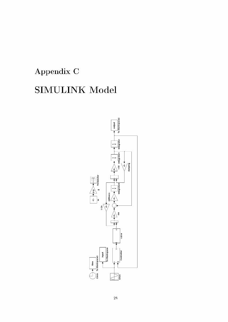
Appendix C

SIMULINK Model

28

Bibliography

[1] Web site Automotive Engineering Science, field of vehicle dynamics, Technische UniversiteitEindhoven, http://www.aes.wtb.tue.nl/english/dynamics.html

[2] Hennekens, D., Schukking, M.: Het operationeel maken van de bandenmeettoren, HTS graduationreport, Hogeschool van Arnhem en Nijmegen, 2005

[3] Teerhuis, P.: Hydraulic Servo Systems, Sheets Fluid Power Transmissions (Course 4N630), Chap-ter 2-5, Technische Universiteit Eindhoven, 2003

[4] Giancoli, D.C.: Physics for Scientists & Engineers, Third Edition, Prentice Hall, pp. 364-367, 2000

29