DESIGN OPTIMIZATION STUDY ON A CONTAINERSHIP...

DESIGN OPTIMIZATION STUDY ON

A CONTAINERSHIP PROPULSION SYSTEM

Brian Cuneo

Thomas McKenney

Morgan Parker

ME 555 Final Report

April 19, 2010

ABSTRACT

This study develops an optimization algorithm to explore the tradeoff between fuel consumption and

engine room volume of a direct drive containership. Standard regression formulas, first principles

analysis and new regression formulas from published manufacturer data are used to formulate a model.

This model is constrained by the data used in the individual regression formulas, physical constraints

and manufacturing capabilities. Each of the subsystems of the total algorithm, hull, propeller and

engine are validated and tested independently to demonstrate feasible solutions. The combined system

uses a sequential approach, hull-propeller-engine, exchanging vectors of interacting variables to

produce an integrated Pareto front between fuel consumption and engine room volume. A test case is

run through the algorithm and the results are examined. With additional data pertaining to routes, fuel

prices and cargo rates, a ship designer could implement this model to find an optimal propulsion system

solution for a given ship speed and displacement. This solution would be subject to scrutiny if the

optimum lies on the subsystem model constraint boundaries, implying different regression models are

required.

Page | 2

Table of Contents

1 Design Problem Statement ................................................................................................................... 5

2 Nomenclature ....................................................................................................................................... 6

3 Hull Optimization Subsystem (Thomas McKenney) .............................................................................. 7

3.1 Mathematical Model .................................................................................................................... 7

3.1.1 Objective Function ................................................................................................................ 7

3.1.2 Constraints .......................................................................................................................... 12

3.1.3 Design Variables and Parameters ....................................................................................... 14

3.1.4 Model Summary .................................................................................................................. 15

3.2 Model Analysis ............................................................................................................................ 16

3.3 Optimization Study ..................................................................................................................... 18

3.3.1 Global Optimality ................................................................................................................ 19

3.3.2 Constraint Activity ............................................................................................................... 19

3.3.3 Case Study ........................................................................................................................... 21

3.4 Parametric Study ......................................................................................................................... 21

3.4.1 Volume Parametric Study ................................................................................................... 21

3.4.2 Ship Speed Parametric Study .............................................................................................. 24

3.5 Discussion of Results ................................................................................................................... 26

4 Propeller Optimization Subsystem (Brian Cuneo) .............................................................................. 28

4.1 Mathematical Model .................................................................................................................. 28

4.1.1 Objective Function .............................................................................................................. 29

4.1.2 Constraints .......................................................................................................................... 30

4.1.3 Design Variables and Parameters ....................................................................................... 32

4.1.4 Model Summary .................................................................................................................. 33

4.2 Model Analysis ............................................................................................................................ 34


Page | 3

4.3 Numerical Analysis ...................................................................................................................... 35


4.4.1 Case Study Introduction ...................................................................................................... 35

4.4.2 Global Optimality and Constraint Activity .......................................................................... 36

4.5 Parametric Study ......................................................................................................................... 37

4.6 Discussion of Results ................................................................................................................... 40

5 Engine Optimization Subsystem (Morgan Parker) .............................................................................. 40

5.1 Mathematical Model .................................................................................................................. 40

5.1.1 Objective Function .............................................................................................................. 41

5.1.2 Constraints .......................................................................................................................... 42

5.1.3 Feasibility ............................................................................................................................ 44

5.1.4 Model Summary .................................................................................................................. 45

5.2 Model Analysis ............................................................................................................................ 45

5.2.1 Boundedness ....................................................................................................................... 45



5.3.1 Implementation .................................................................................................................. 47

5.3.2 Results ................................................................................................................................. 47

5.3.3 Model Validation ................................................................................................................. 50

5.4 Parametric Studies ...................................................................................................................... 52

5.5 Results Discussion ....................................................................................................................... 55

6 System Integration Study .................................................................................................................... 56

6.1 Subsystem Tradeoffs ................................................................................................................... 56

6.2 Methodology ............................................................................................................................... 56

6.3 System Optimization Results ...................................................................................................... 58

6.4 Comparison to Subsystem Optimization .................................................................................... 59

Page | 4

6.5 Integrated System Parametric Study .......................................................................................... 60

6.6 Conclusions ................................................................................................................................. 64

7 Bibliography ........................................................................................................................................ 65

Appendix A Hull Code ............................................................................................................................. 66

1. Hull Optimization Code ....................................................................................................................... 66

2. Hull Objective Function ....................................................................................................................... 66

3. Hull Constraint Function ..................................................................................................................... 70

Appendix B Propeller Code .................................................................................................................... 71

1. Propeller Optimization Code............................................................................................................... 71

2. Propeller Objective Function .............................................................................................................. 72

3. Propeller Constraint Function ............................................................................................................. 74

Appendix C Engine Code ........................................................................................................................ 75

1. Engine Optimization Code .................................................................................................................. 75

2. Engine Objective Function .................................................................................................................. 78

3. Engine Constraint Function ................................................................................................................. 78

1 Design Problem Statement

Containerships are a vital component of the world’s economy. Over 95% of the world’s goods a

transported by sea. With this fact in mind, it can be concluded that an optimized containership design

could provide a major advantage in the industry.

looks like. For this project, the containership’s propulsion system was optimized. A ship’s propulsion

system can be divided into three main subsystems including the hull, propeller, and engine.

worked on the hull subsystem; Brian worked on the propeller subsystem; a

engine subsystem. These distinct systems

ship hull is optimized for speed, volume, resistance and stability.

combination of thrust, open water efficiency and vibration. Marine engines are optimized based on

power, fuel consumption, size, weight and r

weight/volume and speed, were set based on typical containership values

documented methods from a variety of sources to create algorithms that can independently optimize a

hull form, propeller and engine. Once these algorithms are linked, they will share key variables to find a

global optimum. This optimum will target fuel

Figure 1.1: Emma Maersk Containership

There are many trade-offs and competing goals in the ship design process. Some of these inclu

maximizing useable volume while minimizing resistance. Another trade

meets the power and rpm requirements while maintaining low fuel consumption. It is also important to

maximize the propeller efficiency while ensuring pro

more are aspects of the ship design process. This project focus

hull, engine, and propeller of a ship to determine the optimal combination. The optimization at

individual levels was based on analytical models that have been used for decades in the marine industry.

Design Problem Statement

Containerships are a vital component of the world’s economy. Over 95% of the world’s goods a


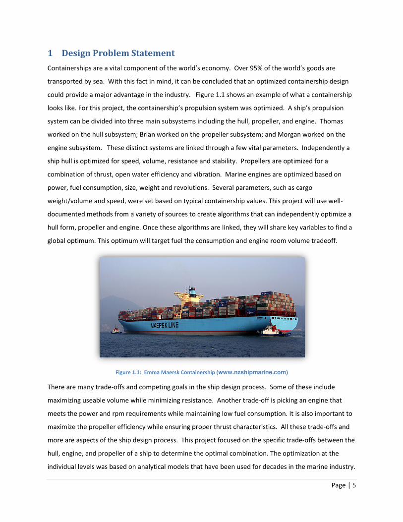
could provide a major advantage in the industry. Figure 1.1 shows an example of what a containership

project, the containership’s propulsion system was optimized. A ship’s propulsion

system can be divided into three main subsystems including the hull, propeller, and engine.

worked on the hull subsystem; Brian worked on the propeller subsystem; and Morgan worked on the

distinct systems are linked through a few vital parameters. Independently a

speed, volume, resistance and stability. Propellers are optimized for a

ater efficiency and vibration. Marine engines are optimized based on

power, fuel consumption, size, weight and revolutions. Several parameters, such as cargo

set based on typical containership values. This project will use w



global optimum. This optimum will target fuel the consumption and engine room volume tradeoff

Emma Maersk Containership (www.nzshipmarine.com)

offs and competing goals in the ship design process. Some of these inclu

maximizing useable volume while minimizing resistance. Another trade-off is picking an engine that


maximize the propeller efficiency while ensuring proper thrust characteristics. All these trade

more are aspects of the ship design process. This project focused on the specific trade

hull, engine, and propeller of a ship to determine the optimal combination. The optimization at

analytical models that have been used for decades in the marine industry.

Page | 5

Containerships are a vital component of the world’s economy. Over 95% of the world’s goods are


shows an example of what a containership

project, the containership’s propulsion system was optimized. A ship’s propulsion

system can be divided into three main subsystems including the hull, propeller, and engine. Thomas

nd Morgan worked on the

linked through a few vital parameters. Independently a

Propellers are optimized for a

ater efficiency and vibration. Marine engines are optimized based on

everal parameters, such as cargo

. This project will use well-



and engine room volume tradeoff.

offs and competing goals in the ship design process. Some of these include

off is picking an engine that


per thrust characteristics. All these trade-offs and

on the specific trade-offs between the

hull, engine, and propeller of a ship to determine the optimal combination. The optimization at the

analytical models that have been used for decades in the marine industry.

Page | 6

The main focus was to integrate these individual models to obtain a global optimization for ship

propulsion.

2 Nomenclature∇ Molded Volume [m3]

1+k1 Form Factor [-]

ABT Transverse Bulb Area [m2]

AE/AO Propeller Expanded Area Ratio [-]

AP Piston Area [m2]

AT Immersed Transverse Transom Area [m2]

AX Max. Transverse Underwater Area [m2]

B Maximum Beam [m]

Bcyl Cylinder Bore [m]

CB Block Coefficient [-]

CF Frictional Resistance Coefficient [-]

CM Midship Coefficient [-]

CP Prismatic Coefficient [-]

CR Residuary Resistance Coefficient [-]

CWP Waterplane Coefficient [-]

D Depth [m]

DP Propeller Diameter [m]

DP Delivered Power [kW]

ERV Engine Room Volume [m3]

EW Engine Weight [MT]

FC Fuel Consumption[MT/h]

FN Froude Number [-]

g Gravitational Constant [m/s2]

HB Vertical Center of Bulb Area [m]

i Number of Cylinders [-]

J Advance Coefficient [-]

K Cavitation Constant [-]

KQ Thrust Coefficient [-]

KT Thrust Coefficient [-]

L Length on Waterline [m]

LCB Longitudinal Center of Buoyancy [m]

LCG Longitudinal Center of Gravity [m]

LR Length of the Run [m]

Ls Length of Stroke [m]

n Propeller Revolutions per Second [1/s]

P,BMEP Brake Mean Effective Pressure [Pa]

P/D Pitch-Diameter Ratio [-]

P0 Pressure at Propeller Hub [-]

PE Engine Effective Power [kW]

PV Water Vapor Pressure [-]

Q Propeller Torque [kN-m]

RA Model-Ship Correlation Resistance [N]

RAPP Appendage Resistance [N]

RB Bulbous Bow Resistance [N]

RBare Bare Hull Resistance [N]

RF Frictional Resistance [N]

RT Required Thrust [-]

RTotal Total Resistance [N]

RTR Immersed Transom Resistance [N]

RW Wave Resistance [N]

SAPP Wetted Area of Appendages [m2]

SFC Specific Fuel Consumption [g/kWh]

T Propeller Thrust [-]

t Thrust Deduction fraction [-]

Tm Average Draft [m]

V Ship Speed [m/s]

VA Speed of Advance [m/s]

w Taylor wake fraction [-]

Z Number of Blades [-]

Δ Displacement [MT]

η0 Propeller Efficiency [-]

μ Kinematic Viscosity [m2/s]

ρ Seawater Density [kg/m3]

Page | 7

3 Hull Optimization Subsystem (Thomas McKenney)

The main goal in hull optimization is to minimize the resistance or drag of the vessel as it travels through

the water, while maintaining a specified displacement. Lower resistance will lead to a smaller power

requirement, which translates to the use of a smaller engine. Although there are basic guidelines for

reducing resistance, there are certain restrictions and considerations that are required to produce a

valid ship design. In general, the longer and more slender a ship’s hull is the less resistance there is.

Making the beam or width of a ship smaller is a good way of reducing resistance. But there are some

consequences if the beam becomes too small or the ship becomes too long. These include stability

issues, freeboard requirements, and reduction in useable volume for cargo.

3.1 Mathematical Model

The objective of the model is to minimize resistance. There are many resistance models that could be

used for this project. Most resistance models are analytical and based on a series of experiments on a

certain type of hull. To ensure that the model is accurate for any given ship, certain similarities are

required. This evaluation is conducted by determining coefficients such as the length-to-beam ratio,

beam-to-draft ratio, or the block coefficient, which describes the underwater hull form. This project will

focus on a basic hull form, used mainly for container ships. One of the most common resistance models

used for these types of ships is the Holtrop and Mennen model. This method is based on regression

analysis of model and full-scale tests of commercial cargo and tanker vessels.

3.1.1 Objective Function

The objective function is based on the Holtrop and Mennen model. All derivations in this section are

from the papers entitled “An Approximate Power Prediction Method” by J. Holtrop and G.G.J. Mennen

published in 1982 and “A Statistical Re-Analysis of Resistance and propulsion Data” by J. Holtrop

published in 1984. The objective function is the resistance equation provided in this paper.

The total resistance of a ship is expressed in Equation 1 below.

�� = �1 + �� + �� + �� + �� + �� + ��

Equation 1

The form factor of the hull uses a prediction formula that is shown as Equation 2 below.

Page | 8

1 + � = ��{0.93 + �� !."�#"$ 0.95 − '��(!.)��##*1 − '� + 0.0225�'��!.,"!,}

Equation 2

The form factor formula includes the parameter LR, which is the length of the run according to Equation

3.

�� = 1 − '� + 0.06'��'�4'� − 1

Equation 3

The coefficient c12 is defined by the following equations depending on the draft to length ratio (T/L).

Draft is the vertical distance from the keel or bottom of the ship to the waterline.

�� = �0� !.��*##, 2ℎ45 0� > 0.05

Equation 4

�� = 48.20 �0� − 0.02 �.!$* + 0.479948 2ℎ45 0.02 < 0� < 0.05

Equation 5

�� = 0.479948 2ℎ45 0� < 0.02

Equation 6

In Equation 4, Equation 5, and Equation 6 the average molded draft is defined as T. The coefficient c13

accounts for the shape of the afterbody and is a function of the coefficient CStern that has a value based

on Table 3.1.

�� = 1 + 0.003':�;<=

Equation 7

Afterbody Form CStern

V-shaped sections -10

Normal section shape 0

U-shaped sections with

Hogner stern 10

Table 3.1: CStern Value Table

Page | 9

The wetted area of the hull can be approximately found using Equation 8.

> = �20 + ��?'@ �0.453 + 0.4425'� − 0.2862'@ − 0.003467�0 + 0.3696'�� + 2.38A��/'�

Equation 8

The appendage resistance can be determined using Equation 9.

�� = 0.5CD�>��1 + ��;E'

Equation 9

Table 3.2 below outlines the approximate values for (1+k2) for given streamlined flow-oriented

appendages. These were determined using resistance tests with bare and appended ship models.

Approximate 1+k2 values

Rudder behind Skeg 1.5 – 2.0

Rudder Behind Stern 1.3 – 1.5

Twin-Screw Balance Rudders 2.8

Shaft Brackets 3.0

Skeg 1.5 – 2.0

Strut Bossings 3.0

Hull Bossings 2.0

Shafts 2.0 – 4.0

Stabilizer Fins 2.8

Dome 2.7

Bilge Keels 1.4 Table 3.2: Approximate 1+k2 Value Table

The equivalent 1+k2 value for all appendages is calculated using Equation 10.

1 + ��;E = ∑1 + ��>��∑ >��

Equation 10

The wave resistance is determined using Equation 11.

�� = ��)∇CG exp {K�LMN + K� cos RLM(�}

Equation 11

The following equations express the coefficients included in Equation 11.

Page | 10

�� = 2223105�$�.$*,��0/��.!$",�90 − ST�(�.�$),)

Equation 12

�$ = 0.229577�/��!.�� 2ℎ45 �/� < 0.11

Equation 13

�$ = �� 2ℎ45 0.11 < �/� < 0.25

Equation 14

�$ = 0.5 − 0.0625�/� 2ℎ45 �/� > 0.25

Equation 15

�� = exp −1.89?��

Equation 16

�) = 1 − 0.8A�/�0'@�

Equation 17

R = 1.446'� − 0.03�/� 2ℎ45 �/� < 12

Equation 18

R = 1.446'� − 0.36 2ℎ45 �/� > 12

Equation 19

K� = 0.0140407�/0 − 1.75254∇��/� − 4.79323�/� − ��,

Equation 20

��, = 8.07981'� − 13.8673'�� + 6.984388'�� 2ℎ45 '� < 0.80

Equation 21

��, = 1.73014 − 0.7067'� 2ℎ45 '� > 0.80

Equation 22

K� = ��)'��exp −.1L=(��

Equation 23

Page | 11

��) = −1.69385 + �/∇�/� − 8.0�/2.36

Equation 24

U = −0.9

Equation 25

The half angle of entrance, iE, is the angle of the waterline at the bow in degrees with reference to the

center plane. It can be approximated using Equation 26.

ST = 1 + 89exp {−�/��!.*!*),1 − '��!.�!#*#1 − '� − 0.0225�'��!.,�,$��/��!.�#)$#100∇/��!.�,�!�}

Equation 26

�� = 0.56A��.)/{�0V0.31?A�� + 0 − ℎ�W}

Equation 27

The additional resistance due to the presence of a bulbous bow near the surface is determined using

Equation 28.

�� = 0.11exp −3X�(�L=Y� A��.)CG/1 + L=Y� �

Equation 28

X� = 0.56?A��/0 − 1.5ℎ�

Equation 29

L=Y = D/ZG0 − ℎ� − 0.25?A�� + 0.15D� Equation 30

Similarly, the additional pressure resistance due to the immersed transom can be determined using

Equation 31.

�� = 0.5CD�A��,

Equation 31

�, = 0.21 − 0.2L=� 2ℎ45 L=� < 5

Equation 32

Page | 12

�, = 0 2ℎ45 L=� ≥ 5

Equation 33

L=� = D/?2GA�/� + �'�� Equation 34

The model-ship correlation resistance can be approximated by Equation 35.

�� = 1/2 D�>'�

Equation 35

'� = 0.006� + 100�(!.�, − 0.00205 + 0.003?�/7.5'�#��0.04 − �#�

Equation 36

�# = 0/� 2ℎ45 0/� ≤ 0.04

Equation 37

�# = 0.04 2ℎ45 0/� > 0.04

3.1.2 Constraints

There are numerous constraints that were be considered for this optimization problem. These

constraints can be grouped into physical constraints and practical constraints. Physical constraints

would include a minimum draft to navigate a canal or enter a harbor or a maximum beam or length to

be able to transit the Panama Canal. Practical constraints would include requiring a certain beam to

ensure stability or dimensions that provide adequate freeboard. There is a third type of constraint for

this particular problem. There are restrictions of the resistance model, which are based on the types of

hull forms used to develop the model. All constraints used in this problem are provided below.

T ≤ 15 m (Draft limit for Port of Los Angeles and Panama Canal)

L ≤ 366 m (Length limit for Panama Canal)

B ≤ 49 m (Beam limit for Panama Canal)

0.0 ≤ D/√LWL ≤ 2.0 (Speed to Length Ratio Criteria for Holtrop Model)

0.01 ≤ V/?gLbc ≤ 0.55 (Froude Number Criteria for Holtrop Model)

Page | 13

2.1 ≤ B/T ≤ 4.0 (Beam to Draft Ratio Criteria for Holtrop Model)

0.55 ≤ ∇/LbcAe� ≤ 0.85 (Prismatic Coefficient Criteria for Holtrop Model)

3.9 ≤ LWL/B ≤ 14.9 (Length to Beam Ratio Criteria for Holtrop Model)

D – T ≥ 4 (U.S. Coast Guard Required Freeboard)

GMT ≥ 0.5 (U.S. Coast Guard Wind Heel Stability Requirement)

B/D ≥ 1.65 (Additional Stability Requirement)

CB ≥ 0 (Block Coefficient Lower Bound)

L∙B∙T∙CB=∇ (Volume Equality Constraint)

The variables were also bounded at the lower end with values of zero. None of the dimensions of the

ship can be negative. The length, beam, and draft have upper bounds based on access to ports and

canals. The upper bound of the block coefficient is one, because it is a ratio and can only be between

zero and one. The depth is defined as the vertical distance from the keel to the main deck. The depth

has a lower bound from the required freeboard constraint. The upper bound was set for well

boundedness as 50 m in the optimizer. The optimizer will never output a value this high mainly because

the depth would like to be minimized by the stability requirement.

The U.S. Coast Guard Wind Heel Stability Requirement is based on some basic naval architecture

principles and regression equations. The details of the GMT calculations are provided below.

'f� = '�/'��

g� = 0h � '��'� + '��

gi = 0.7j

'Y = 0.0937 ∗ '� − 0.0122

l� = 'Y ∗ ��m ∗ ��m�

�n = l�∇

Page | 14

gn = g� + �n

in� = gn − gi

3.1.3 Design Variables and Parameters

The design variables for this optimization define the basic dimensions and shape of the ship hull. From

these variables, approximate calculations can be completed to determine design considerations and

determine if a design is feasible. The list of design variables is provided below.

• T, Mean Draft

• L, Length on Waterline

• B, Maximum Beam

• CB, Block Coefficient

• D, Depth

The design parameters also play an important role in this optimization and are listed below. Also

provided are example values or ranges for the parameters.

• VS, Speed of the Ship [10 – 13.5 m/s]

• ∇, Molded Volume [10,000 – 100,000 m3]

• CWP, Waterplane Coefficient [0.7 – 0.9]

• CM, Midship Coefficient [0.7 – 0.9]

• LCB, Longitudinal Center of Buoyancy [±5% from amidships]

• ATR, Submerged Transom Area [0 – 30 m2]

• CSTERN, Stern Shape [-25 – 10]

• SAPP, Appendage Area [0 – 100 m2]

• ABT, Transverse Area of Bulb [0 – 50 m2]

• HB, Center of Bulb Area [0 – 10 m]

Page | 15

3.1.4 Model Summary

Objective Function: max q = ��, �, 0� ∗ 1 + �� + ��'�� + ��, �, 0� + ��0� + ��, '�� + ��, 0, '��

Subject to:

G� = 0 − 15 ≤ 0

G� = � − 366 ≤ 0

G� = � − 49 ≤ 0

G# = − D√LWL ≤ 0

G) = D√LWL − 2.0 ≤ 0

G, = 0.01 − D√gLWL ≤ 0

G$ = D√gLWL − 0.55 ≤ 0

G* = 2.1 − �0 ≤ 0

G" = �0 − 4.0 ≤ 0

G�! = 0.55 − ∇�As� ≤ 0

G�� = ∇�As� − 0.85 ≤ 0

G�� = 3.9 − �� ≤ 0

G�� = �� − 14.9 ≤ 0

G�# = 4 − j + 0 ≤ 0

G�) = 0.5 − in� ≤ 0

G�, = 1.65 − �j ≤ 0

G�$ = −'� ≤ 0

ℎ� = � ∗ � ∗ 0 ∗ '� − ∇= 0

Page | 16

3.2 Model Analysis

Before attempting to implement the optimization problem, it is important to evaluate the objective

function and constraints to see if any information about the problem can be extracted. A common

method used to evaluate models is monotonicity analysis. This analysis can be used to validate that the

problem is well bounded with respect to every variable as well as determine possibly active constraints.

The application of monotonicity analysis for optimization problems is only possible under certain

conditions. For resistance optimization, the monotonicity of the objective function is unknown. This is

because the total resistance is a combination of different types of resistance that incorporate the

variables with various monotonicities. It cannot be determined if the objective function is increasing or

decreasing with respect to any of the variables. Although the monotonicity of the objective function

cannot be completed, the constraints can still be evaluated to prove well boundedness of the problem.

Monotonicity analysis was completed for all constraints. Each variable has at least one upper and lower

bound. This was determined by showing that there are both increasing and decreasing constraints with

respect to every variable. Table 3.3 below shows the monotonicity table for all the constraints. The plus

sign signifies that the constraint is increasing with respect to the variable. The minus sign signifies that

the constraint is decreasing with respect to the variable. The dots signify that the variable is not

included in the given constraint. The stars after the plus or minus signs signify that the given constraint

is active with respect to that variable. Most of the variables were present in multiple constraints, which

mean that active constraints could not be readily determined.

Page | 17

Table 3.3: Monotonicity Table for Constraints

The block coefficient and depth are the two variables that the most information can be determined from

the monotonicity analysis. The block coefficient is bounded by inequality constraint 15 (GMT stability

constraint). Although inequality constraint 17 bounds the block coefficient at the lower bound, it will

never reached this bound because the equality constraint requires a certain volume value, which cannot

be achieved when the block coefficient is zero. The depth variable is not present in the objective

function. It is, however, a very important dimension of a ship and was used for many calculations. The

depth plays a role in stability calculations as well as freeboard requirements. It can be seen in Table 3.3

that the depth was constrained by inequality constraint 14, which is the required freeboard constraint.

This constraint was active with respect to the depth because the freeboard should be pushed to its

minimum based on the other constraints. At least one of inequality constraints 15 and 16 was also

active with respect to depth.

Due to many of the variables having multiple increasing and decreasing roles in the constraints, it was

worth evaluating the constraints further to determine if any are redundant. This can be very difficult

when there are more than one or two variables because of the design space in multiple dimensions.

Page | 18

Some basic conclusions were made for a few constraints that seem to be related. After evaluating

inequality constraints 4 through 7, there seems to be possible redundancies. It can be determined that

inequality constraint 4 was not needed because inequality constraint 6 reached its lower bound first.

The same can be concluded for the upper bounds in inequality constraints 5 and 7. Inequality constraint

7 was not needed because inequality constraint 5 reached its upper bound first.

It is very difficult to determine any additional information from the monotonicity analysis. It can be

concluded that the optimization problem is well bounded and should output valid optimal results.

3.3 Optimization Study

Due to the fact that the resistance objective function was smooth and could be calculated very fast,

MATLAB was used as the optimization tool. The fmincon function was used to implement the gradient

based method used to determine the optimal solution. Three MATLAB files were generated: one that

calculated the objective function, one that had all the constraints, and a third that ran the optimization.

These files are included in Appendix A.

The results of the optimization problem mainly focus on the trends of how the principle dimensions of

the ship change as both the speed and volume vary, which will be discussed further in the next section.

One optimal solution for this problem would not be that meaningful. The test values used as

parameters were decided based on similar ship data. If an actual design of a ship was being completed,

more detailed information would be required to set the parameter values. This is why the main focus

for the results analysis was on the parametric study completed. The two most influential parameters

were the speed and volume of the ship. Both studies produced general trends that are logical based on

engineering judgment. The specific changes in the variables were more interesting as well as their

association with which constraints were active for all the parameter values. One of the most interesting

and unexpected occurrences is how the active constraints changed as the parameter values were

altered.

In order to fully understand the design space and what factors impacted the optimal solution, certain

tests were completed. The following subsections include example results for certain situations including

determining global optimally, constraint activity, as well as a case study that was completed using the

same values for all subsystems.

Page | 19

3.3.1 Global Optimality

Due to the smooth nature of the objective function and the constraints, it was determined that a global

optimum could be obtained using a gradient based or line search method. To verify these assumptions,

the model was started at various points in the design space. The results show that regardless of the

starting point, the final optimal solution is the same. This can be seen in Table 3.4 below. Various

starting points from the lower and upper bounds of all the variables were used. The same resulting

optimal solution proves that a global optimum can be found using the gradient based method utilized in

MATLAB. If all the resulting optimal solutions were not the same, this would lead to the conclusion that

there are multiple local optimums.

Table 3.4: Optimal Solution for Various Starting Points

3.3.2 Constraint Activity

Based on general naval architecture principles, it was hypothesized that the active constraints for this

problem would be the constraints associated with stability. This is because the resistance model can

reduce the resistance dramatically by making the ship narrower. The stability of the ship is directly

related to the beam or width of the ship. From these two statements, it could be concluded that the

stability requirements would most likely be the active constraints for this problem. Monotonicity

analysis also indicted that the stability constraints would most likely be active, at least for certain

variables.

The two main stability requirements are inequality constraints 14 and 15. Inequality constraint 14 sets a

required value for the freeboard (vertical distance from the waterline to the main deck). This value

would most likely be pushed to its limit because of the depth’s role in stability calculations. As the

freeboard increases, the depth also increases. The overall center of gravity of the ship usually increases

Page | 20

as the depth increases. A higher center of gravity translates to a less stable ship, which is taken into

account in inequality constraint 15. The GMT is a value that determines the upright stability of the ship.

A GMT value greater than zero means that the ship is stable. That value is usually increased based on

additional heel caused by wind. This is the only constraint that involves every variable.

Another major driver in this problem was the volume equality constraint, which is directly related to

displacement. If this constraint was not included, the optimizer would simply reduce the dimensions of

the ship, which would in turn reduce the resistance. This is not a meaningful result because ships are

designed for a purpose. In most cases their purpose involves carrying a specific amount of cargo. This

equality constraint only allows the hull form to change size while maintaining the same volume or

displacement.

After running the optimizer for varies conditions, the hypothesis made earlier in regards to the stability

constraints being active was generally correct. There was, however, an occurrence that was not

predicted. Other than the two stability constraints, there were other active constraints. The two other

constraints encountered were restrictions set by the model. This means that the optimizer wanted to

go outside the ranges that the model was valid for. In order to determine exactly how these active

constraints were limiting the optimal solution, the model constraints were removed and the optimizer

was run without them. The new result led to larger values for all the dimensions and a decrease in the

block coefficient. This means that the ship overall became larger, but the underwater shape was not as

full. Although this does have a better resistance, the shape of the hull no longer matches the shapes

used for the model, which makes that result invalid. Table 3.5 shows example outputs with and without

the model constraints. It can be concluded that if a wider range of hull form options is desired, another

resistance model would be required.

Table 3.5: Optimal Solutions With and Without Model Constraints

Based on constraint activity analysis, it can be concluded that there will always be at least one active

constraint for this individual subsystem. This means that all optimums are boundary solutions. Interior

optimums do occur, however, during the system integration. The details of the results of the system

integration will be discussed later in this report.

Page | 21

3.3.3 Case Study

A case study was completed using the same parameter values for all subsystems. This was completed so

the final integrated results could be compared to the individual optimal solutions obtained from each

subsystem. The main parameters that were set include the ship speed, which was set at 18 knots, and

the molded volume, which was set at 75,000 cubic meters. Both values are typical for containerships

and produce valid results from all subsystems. The results of the case study are provided below in Table

3.6.

Table 3.6: Optimal Solution of Case Study

The results of this case study show ship dimensions closer to their upper bounds. This is mainly due to

the large parameter values used for volume and speed. It can also be seen that the two active

constraints are the required freeboard and stability requirement. This shows that for the parameter

values selected, the model is obtaining a true optimum within the model limits and the typical

constraints are active.

3.4 Parametric Study

A parametric study was completed for this project. The two parameters that were evaluated were the

ship speed and molded volume. The optimal results were evaluated as these two parameters were

varied within a reasonable range. The active constraints were also evaluated as these parameters

changed. Because detailed information on a specific ship was not used for this project, one optimal

solution could not be obtained. The parametric study does show how the optimal hull would change as

key parameters such as speed and volume change.

3.4.1 Volume Parametric Study

The first parameter that was varied for this study was the molded volume. The molded volume is the

volume of the hull under the waterline. This value can be multiplied by the density of water to obtain a

displacement, or weight, of the ship. The volume was varied between 20,000 and 40,000 m3. This range

corresponds to a typical medium-sized containership. Although volume is being considered as a

parameter for this study, it is truly an equality constraint in the optimization. Because it is an equality

constraint, it must always be met by the optimal result. Equality constraints like these should be

evaluated at various values to fully understand their impacts. Table 3.7 shows the results of the

parametric study for volume. The table shows the volume value and its associated displacement, the

optimal solution with resistance value, and the active constraints for each solution.

Table 3.7: Parametric Study Results for the Volume Parameter

To help evaluate the results of the parametric study, a series of graphs were produced for the resistance

of each solution as well as one for each variable.

parametric study for volume.

Figure 3.1: Resistance and Draft Curves for Volume Parametric Study


optimal solution with resistance value, and the active constraints for each solution.

: Parametric Study Results for the Volume Parameter


of each solution as well as one for each variable. Figure 3.1 through Figure 3.3 shows the graphs of the

Resistance and Draft Curves for Volume Parametric Study

Page | 22



the graphs of the

Figure 3.2: Length and Beam Curves for Volume Parametric Study

Figure 3.3: Depth and Block Coefficient Curves for Volume Parametric Study

It can be seen from the results of the parametric study

increases. The only variable that does not increase is the block

general trend of the principle dimensions correspond to the increased volum

the molded volume, the dimensions of the ship must increase to

From the resistance curve, it can also be seen that the resistance increases linearly with volume. This

also makes sense because the added volume will cause the resistance to increase.

beam curves are relatively linear as the volume varies.

a value of 0.54. This variable most likely remained constant due to a lower

translating to a lower resistance. The value of 0.54 was the lowest value allowed by the active

constraint, which was the prismatic coefficient lower limit.

the remaining variables would then have to be increased to meet the changing volume requirement.

The one variable that had very unexpected results was the depth.

active, the depth should follow the same trend as the draft, but at higher values.

study, the freeboard constraint was only active for the first five values for the volume.

Length and Beam Curves for Volume Parametric Study

Depth and Block Coefficient Curves for Volume Parametric Study

the parametric study that most of the variables increase as the volume

increases. The only variable that does not increase is the block coefficient, which remains constant. The

general trend of the principle dimensions correspond to the increased volume requirement. To increase

the molded volume, the dimensions of the ship must increase to accommodate the added volume.


added volume will cause the resistance to increase. The draft, length, and

beam curves are relatively linear as the volume varies. The block coefficient remained constant around

a value of 0.54. This variable most likely remained constant due to a lower block coefficient always

to a lower resistance. The value of 0.54 was the lowest value allowed by the active

constraint, which was the prismatic coefficient lower limit. Due to the block coefficient not changing,

d then have to be increased to meet the changing volume requirement.

The one variable that had very unexpected results was the depth. When the freeboard constraint is

active, the depth should follow the same trend as the draft, but at higher values. During this parametric

study, the freeboard constraint was only active for the first five values for the volume.

Page | 23

that most of the variables increase as the volume

coefficient, which remains constant. The

e requirement. To increase

the added volume.


The draft, length, and

The block coefficient remained constant around

ck coefficient always

to a lower resistance. The value of 0.54 was the lowest value allowed by the active

Due to the block coefficient not changing,

d then have to be increased to meet the changing volume requirement.

When the freeboard constraint is

ng this parametric

The lower

portion of the depth curve does show the same trend as the draft variable, but becomes very non

after the freeboard constraint is no longer active.

the depth could be multiple values if unconstrained by the freeboard requirements

values could have been determined by the values that meet the stability require

mentioned previously in this report, the prismatic coefficient constraint was active for most of the

results. For this parametric study, it was active for all solutions.

being pushed to the limits of the type of

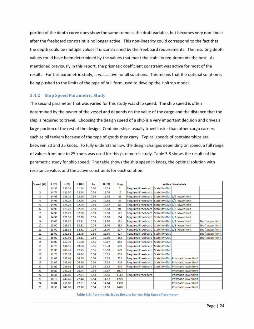
3.4.2 Ship Speed Parametric Study

The second parameter that was varied for this study was ship speed.

determined by the owner of the vessel and depends on the value of the

ship is required to travel. Choosing the design speed of a ship is a very important decision and drives a

large portion of the rest of the design. Containerships usually travel faster than other cargo carriers

such as oil tankers because of the type of goods they carry. Typical speeds of containerships are

between 20 and 25 knots. To fully understand how the design changes depending on speed, a full range

of values from one to 25 knots was used for this parametric study.

parametric study for ship speed. The table shows the

resistance value, and the active constraints for each solution.

Table 3.8: Parametric Study Results for the Ship Speed Parameter

portion of the depth curve does show the same trend as the draft variable, but becomes very non

no longer active. This non-linearity could correspond to the fact that

the depth could be multiple values if unconstrained by the freeboard requirements. The resulting depth

values could have been determined by the values that meet the stability requirements the best.


results. For this parametric study, it was active for all solutions. This means that the optimal solution is

the type of hull form used to develop the Holtrop model.

Ship Speed Parametric Study

The second parameter that was varied for this study was ship speed. The ship speed is often

determined by the owner of the vessel and depends on the value of the cargo and the distance th

. Choosing the design speed of a ship is a very important decision and drives a


tankers because of the type of goods they carry. Typical speeds of containerships are

To fully understand how the design changes depending on speed, a full range

of values from one to 25 knots was used for this parametric study. Table 3.8 shows the results of the

parametric study for ship speed. The table shows the ship speed in knots, the optimal solution with

resistance value, and the active constraints for each solution.

: Parametric Study Results for the Ship Speed Parameter

Page | 24

portion of the depth curve does show the same trend as the draft variable, but becomes very non-linear

linearity could correspond to the fact that

. The resulting depth

ments the best. As


This means that the optimal solution is

The ship speed is often

cargo and the distance that the

. Choosing the design speed of a ship is a very important decision and drives a


tankers because of the type of goods they carry. Typical speeds of containerships are

To fully understand how the design changes depending on speed, a full range

shows the results of the

the optimal solution with


of each solution as well as one for each variable.

parametric study for ship speed.

Figure 3.4: Resistance and Draft Curves for Ship Speed Parametric Study

Figure 3.5: Length and Beam Curves for Ship Speed Parametric Study

Figure 3.6: Depth and Block Coefficient Curves for Ship Speed Parametric Study

The resistance curve shows the basic relationship between speed and resistance for ships.

variables seem to change dramatically at certain speed values.

active constraints for the optimal solutions as the speed changes.

constraints is that the freeboard and stability constraint


of each solution as well as one for each variable. Figure 3.4 through Figure 3.6 are the graphs of

Resistance and Draft Curves for Ship Speed Parametric Study

Length and Beam Curves for Ship Speed Parametric Study

Depth and Block Coefficient Curves for Ship Speed Parametric Study

curve shows the basic relationship between speed and resistance for ships.

variables seem to change dramatically at certain speed values. These changes can be related to the

active constraints for the optimal solutions as the speed changes. The first trend in the active

constraints is that the freeboard and stability constraints are active from one knot to 20 knots.

Page | 25


the graphs of the

curve shows the basic relationship between speed and resistance for ships. Also, the

These changes can be related to the

he first trend in the active

are active from one knot to 20 knots. These

Page | 26

two constraints do not have a major impact in the change in dimension values though. The freeboard

and stability constraints do affect the results from 20 to 25 knots because they are no longer active. The

prismatic coefficient constraint then becomes active, which means that the optimal ship is pushing the

limits of the model. This changeover in active constraints made the draft and depth decrease and the

length and beam increase slightly. The block coefficient remains constant for this range, which is similar

to the volume parametric study when the prismatic coefficient constraint was active.

The major changes in the results occur when the length to beam ratio constraint and the draft upper

limit constraints were active. An initial trend can be seen for the first two speed values, but is stopped

when the length to beam ratio constraint became active. This constraint being active caused all

variables to remain relatively constant. This occurs because with the length to beam ratio being set, the

values of length and beam do not change much. With the length and beam not changing, the draft and

depth must remain at the same values also to maintain the required volume. Between 9 and 13 knots

the draft upper limit constraint became active. This in turn set the draft and depth, which translated to

the length and beam not varying that much to maintain the required volume. At around 13 knots, all

variables change dramatically. At this point, only the freeboard and stability constraints were active. In

general, as the speed increases a more slender hull form would have better resistance. This means that

the length would increase and the beam would decrease. Draft would also decrease as speed increased

to have better resistance. The block coefficient would decrease to generate a more slender hull. This

trend can be seen in the results, but to a dramatic degree. It can be seen that changing active

constraints play a major role in the optimal solution.

The Holtrop model seems to play a restrictive role in finding the true optimal solutions. It can be seen

that between 18 and 25 knots that the solution is constrained by the model limits. It is important to

note that when the Holtrop model was developed, the ships were not designed to go at higher speeds

greater than 20 knots. Because none of the hulls used for the model were designed to go this fast, it can

be concluded that these hulls might not be the optimal designs for these higher speeds. This idea is

reinforced by the results of this parametric study. The active constraints at these higher speeds are

related to the limits of the model, not the typical freeboard and stability requirements.

3.5 Discussion of Results

The results of the parametric studies show how important active constraints are in the resulting optimal

solutions. Although the predicted trends could be seen in the resulting data, the optimal solutions were

Page | 27

restricted by other considerations. The results of this optimization study show that a better model

incorporating present day considerations such as larger volumes and higher speeds should be used to

determine the true optimal designs. It can be seen that optimal solutions are moving towards finer hulls

under the waterline. The Holtrop model was developed in the early 1980s and was revised over the

next decade. The revisions came from evaluations of inconsistencies with the model and additional

tests were completed to change the model. These revisions did not continue into the 1990s and further.

For future work in this area, it is recommended that another model be used for resistance calculations

such as the Hollenbach method.

Basic fundamentals in ship design are still proven important by the results as the freeboard and stability

constraints played a major role in the optimal solutions. It was predicted that the model would want to

make the ship as slender as possible. If the stability constraint was not included, the ship would be very

long, narrow and very unstable. The stability constraint allowed the optimal solution to be as slender as

possible while still maintaining proper stability. A stability check is always an essential part of the design

of a ship. This optimizer automates this design step and iterates many designs to find the best possible

solution as opposed to simply a feasible one. The freeboard requirement is also very important.

Freeboard is required to protect the ship from being swamped by having water come over the main

deck. Also, freeboard is closely related to reserve buoyancy. Reserve buoyancy is important because if

the ship was damaged and took on water, the added buoyancy from a higher waterline would

counteract the flooding and stabilize the ship.

The optimization could be improved by adding additional constraints such as maneuvering or

seakeeping requirements. A hull could also be optimized for maneuvering and seakeeping instead of

considering them constraints. A tradeoff between resistance, maneuvering, and seakeeping would be

an additional and more complete analysis to complete a hull optimization. Maneuvering and

seakeeping are much harder to model than resistance and have no empirical models that simplify the

analysis. In most cases these two calculations are completed using highly nonlinear and complicated

models. Simplified constraints could be developed, but would not incorporate the full extent of these

calculations.

Page | 28

4 Propeller Optimization Subsystem (Brian Cuneo)

To achieve the maximum fuel efficiency for the hull-propeller-engine system, the propeller efficiency

was maximized. The final propeller design provided the necessary thrust to meet the design speed of

the ship.

The propulsion system of a ship can have many forms however for the design of this system choices

were limited to Wageningen B-Series Propellers. B-Series Propellers have become very popular for ships

with fixed pitch propellers due to the variety of blade number, pitch to diameter ratios, and expanded

area ratios that are available. Design variables for B-Series propellers include speed of advance,

expanded area ratio, pitch to diameter ratio, and the number of propeller blades. The main input

parameters for the optimization problem include the thrust required to maintain design speed, the

diameter that fits under the hull and the rpm and torque provided by the engine.

The interaction between hull, propeller and engine introduces trade-offs that must be made if all sub-

systems are to be optimized for maximum fuel efficiency. The diameter of the prop is restricted by the

hull. A larger diameter propeller increases propeller efficiency, however, the hull draft is restricted by

port depths and stability issues. Also the input shaft rpm of the engine influences the maximum

diameter that can be used for the propeller due to cavitation concerns that is a function of propeller

blade tip speeds.


The optimal propeller design for fuel efficiency is to maximize the propeller efficiency behind the hull of

the ship. This optimization is dependent on coefficients of torque and thrust, which are determined by

the hull shape and the properties of the engine. For B-Series propellers a model has been developed by

Bernitsas and Ray. Propeller optimization must meet the requirements for thrust to meet the speed

that the owner has specified using the power that is delivered by the engine. Figure 4.1 displays a graph

of the objective function versus the advance coefficient. This graph is for a fixed blade number (4) and

fixed expanded area ratio (0.6) with different lines representing pitch to diameter ratios.

Many assumptions were made in this model to allow for simplification of calculations while still

producing meaningful results. First, the Taylor wake fraction, and thrust deduction coefficient are

considered constant for all iterations of the hull. While this is not completley accurate, because the

same hull type and clearances are used for all runs, the results are reasonable as the two coefficients

would change very little between cases. Another main assumption is that no efficiencies are used

Page | 29

between the propeller and engine. As there is no reduction gear used this becomes more accurate, but

the missing efficiencies would have the same effect on all iterations of the optimization code. So this

may affect the final value of the objective function, but the optimum design variables will be the same.

Figure 4.1: Wageningen B-Series Chart


The standard mathematical model for the optimization problem can be written as follows in Equation

38, where η0 is a function of KT, KQ, and J as shown in Equation 39. The values for KT and KQ in terms of

the design variables are found using experimental results. The experimental data gives coefficients and

exponents to Equation 40 and Equation 41, which can be found in “KT, KQ and Efficiency Curves for the

Wageningen B-Series Propellers” and in the code implementation shown in Appendix B .

KtuSKSv4 w0

= qx , Xj , AyAz , {� Equation 38

w| = xg�2}g~ Equation 39

g� = � '�,�,�,�� ∗ x�� ∗ Xj�� ∗ ATA|�� ∗ {��

Equation 40

Page | 30

g~ = � '�,�,�,�~ ∗ x�� ∗ Xj�� ∗ ATA|�� ∗ {��

Equation 41

4.1.2 Constraints

The model is constrained by several physical and practical constraints. The diameter is constrained to

being less that a constant, a, determined by the hull shape and necessary hull clearances shown in

Equation 42. The advance coefficient design variable is defined by the speed of advance, the shaft

revolutions per second, and the propeller diameter set by the ship speed, hull form, and engine

revolution per second as shown in Equation 43. The thrust from the propeller is related to the required

thrust to make the ship speed by Equation 46.

j ≤ t

Equation 42

x = D�5j

Equation 43

g� = 0C5�j# Equation 44

g~ = jX2}C5�j) Equation 45

�� = 01 − ��

Equation 46

For the model, to ensure that the propeller rpm and diameter are constant in the dimensionless

coefficients, Equation 43, Equation 44, and Equation 45 are combined into two non-linear constraints

which are shown below.

0 = 0 ∗ x�C ∗ j� ∗ D�� − g�

Equation 47

Page | 31

jX ∗ x�2}Cj�D�� − g~ ≤ 0

Equation 48

Equation 48 is an inequality constraint because the power needed to overcome the resistance may be

less than the max power that is supplied by the engine. Equation 48 is not used as a constraint because

the engine was matched to the necessary thrust. The model can also be used to maximize the speed for

a given engine. If this is the case, Equation 48 is active.

Another problem when dealing with propeller efficiency optimization is cavitation concerns. The

following constraint is placed on the blade expanded area ratio to prevent cavitation based on the

propeller diameter, the water pressure at the propeller hub, and the thrust provided by the propeller.

ATA| − 1.3 + 0.3 ∗ {�0X| − Xf�j� − g ≤ 0

Equation 49

Where P0 is the static pressure at the propeller hub, PV is the vapor pressure of water, and K is a

constant depending on ship type for a single screw vessel K is 0.2. (Van Manen & Van Oossanen, 1988)

The following six constraints are practical constraints required by the Wageningen B-Series Propellers.

The first two practical constraints are for the blade number which must be an integer value. The next

two constraints are required for the expanded area ratio of the B-Series propeller. Outside of the range

given for expanded area ratio the experimental data for the thrust coefficient and torque coefficient is

no longer reliable. The final requirements by the Wageningen B-Series model are placed on the pitch to

diameter ratio. Again, outside of the given range the experimental data equations are no longer

reliable.

2 − { < 0

Equation 50

{ − 8 < 0

Equation 51

Page | 32

0.30 − ATA| ≤ 0

Equation 52

ATA| − 1.05 ≤ 0

Equation 53

0.5 − Xj ≤ 0 Equation 54

Xj − 1.40 ≤ 0

Equation 55

4.1.3 Design Variables and Parameters

The optimization design variables for propeller optimization are mainly dimensionless values used to

describe the blade shapes and angles. The dimensionless values depend on parameters that are

dependent on the other subsystem which induces coupling in the optimization process. These variables

are listed below.

• Speed of Advance (J)

• Pitch to Diameter Ratio (P/D)

• Expanded Area Ratio (AE/AO)

• Number of Blades (Z)

The main parameters that are used in the propeller optimization system are listed below.

• Required Thrust (RT)

• Ship Speed (VS)

• Maximum Propeller Diameter (D)

Page | 33

4.1.4 Model Summary

Objective Function:

KtuSKSv4 w0

= qx , Xj , AyAz , {� = xg02}g� Where:

g� = � '�,�,�,�� ∗ x�� ∗ Xj�� ∗ ATA|�� ∗ {��

g~ = � '�,�,�,�~ ∗ x�� ∗ Xj�� ∗ ATA|�� ∗ {��

Subject To: ℎ� = 0 ∗ x�

C ∗ j� ∗ D�� − g� = 0

G� = ATA| − 1.3 + 0.3 ∗ {�0X| − Xf�j� − g ≤ 0

G� = jX ∗ x�2}Cj�D�� − g~ ≤ 0

G� = −x ≤ 0

G# = 2 − { < 0

G) = { − 7 < 0

G, = 0.30 − ATA| ≤ 0

G$ = ATA| − 1.05 ≤ 0

G* = 0.5 − Xj ≤ 0 G" = Xj − 1.40 ≤ 0

Page | 34

4.2 Model Analysis

Before running the optimization code the model was examined for well boundedness by using

monotonicity analysis. Due to the complexity of the objective function, monotinicities could not be

determined. This required all of the variables to be well bounded in the constraints.

Table 4.1 shows the montonicity table for the optimization problem. The table shows that all of the

design variables are bounded by the physical limitations of the model used for analyses, so from

monotonicity principle one the problem is well bounded.

J P/D AE/A0 Z

f

h1 +

g1 + -

g2 +

g3 -

g4 -

g5 +

g6 -

g7 +

g8 -

g9 +

Table 4.1 Monotonicity Table


Activity of the constraints is difficult to determine due to the lack of information surrounding the

objective function. The pitch to diameter ratio is bounded by active constraints g8 and g9. The speed of

advance is constrained by h1 and g3. The expanded area ratio is constrained by the conditionally critical

set of g1, g6, and g7. The blade number is constrained by the conditionally critical set of g1, g4, and g5.

Ane of changing active constraints can be seen in the case study in section 4.4. In the example provided

the following constraints are active depending on the blade number being examined:

Page | 35

Blade Number (Z) Active Constraints

3 h1,g6

4 h1,g6,g9

5 h1,g1

6 h1,g1

7 h1,g9,g7

Table 4.2: Constraint Activity

4.3 Numerical Analysis

The optimization algorithm was then run for a test case to find an optimal value for a given ship and

engine. The optimization algorithm used was a version of an active set algorithm found in MATLAB’s

fmincon function. The constraints in the optimization method require tradeoffs between the other two

subsystems of the hull-propeller-engine optimization problem. Either the required thrust from the hull

or the delivered horsepower from the engine can be the factor that most influences the propeller

efficiency. A parametric study was done to see the effects of changing the resistance and delivered

power.


4.4.1 Case Study Introduction

A case study was analyzed to see if the model successfully found an optimum for realistic parameters for

a ship. The case study was done for a preselected volume of 75,000 m3 and ship speed for 18 knots.

The volume and ship speed were used to find an optimum resistance. The optimal resistance was input

to the propeller optimization along with the corresponding draft. The following data was used for the

optimization:

Draft = 14.64 [m]

D = 10.25 [m]

VS = 18 [knots]

RT = 1036.5 [kN]

t = 0.155 [-]

w = 0.252 [-]

When this data is entered into the optimization code, the following optimums were obtained for each

blade number.

Page | 36

Blade Number (Z) J P/D AE/A0 η0

3 0.7998 1.0547 0.3 0.7230

4 0.9951 1.4 0.3 0.7091

5 0.9372 1.2552 0.6231 0.6997

6 0.962 1.2826 0.7429 0.6989

7 1.0262 1.4 1.05 0.7148

Table 4.3: Test Case Results

From Table 4.3 the overall optimum is a 3 blade prop with P/D of 1.05, AE/A0 of 0.3, and operating at J of

0.800. This combination of design variables results in an ηo of 0.723. With this propeller, the thrust

required to overcome the resistance can be accomplished with a delivered power of 28,650 kW. The

engine would be required to operate at a speed of 0.845 rps if no reduction gear is used, which would

increase the required power due to losses in gearing efficiency.

4.4.2 Global Optimality and Constraint Activity

Multiple starting points were examined to check for global versus local optimum. Table 4.4 shows a

sample of results of starting from multiple points. All runs converged to the same point indicating a

global maximum.

J0 P/D0 (AE/A0)0 η0 max

0.1 0.5 0.3 0.7230

0.4 0.85 0.9 0.7230

0.6 0.6 0.10 0.7230

0.5 1.4 1.05 0.7230

Table 4.4: Results for Multiple Starting Points

For the optimal case, the constraint activity is examined. The overall optimum is constrained by the

model constraint on AE/AO, blade number, and the thrust constraint h1. Propellers are most efficient

with the smallest number of blades, and small expanded area ratios, so these results are to be expected

if the cavitation constraint is not active. As the blade number is increased, the cavitation becomes

active for blade numbers 5 through 7.

How the constraints affect the optimization problem can be examined by relaxing the different

constraints. When the equality constraint on thrust is removed, the program can find the optimal

efficiency for a given draft. Table 4.5 shows the results of running the optimization program with the

Page | 37

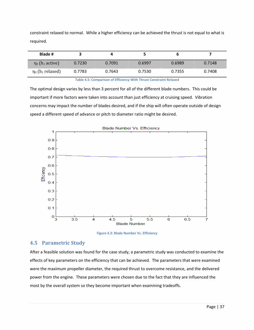
constraint relaxed to normal. While a higher efficiency can be achieved the thrust is not equal to what is

required.

Blade # 3 4 5 6 7

η0 (h1 active) 0.7230 0.7091 0.6997 0.6989 0.7148

η0 (h1 relaxed) 0.7783 0.7643 0.7530 0.7355 0.7408

Table 4.5: Comparison of Efficiency With Thrust Constraint Relaxed

The optimal design varies by less than 3 percent for all of the different blade numbers. This could be

important if more factors were taken into account than just efficiency at cruising speed. Vibration

concerns may impact the number of blades desired, and if the ship will often operate outside of design

speed a different speed of advance or pitch to diameter ratio might be desired.

Figure 4.2: Blade Number Vs. Efficiency

4.5 Parametric Study

After a feasible solution was found for the case study, a parametric study was conducted to examine the

effects of key parameters on the efficiency that can be achieved. The parameters that were examined

were the maximum propeller diameter, the required thrust to overcome resistance, and the delivered

power from the engine. These parameters were chosen due to the fact that they are influenced the

most by the overall system so they become important when examining tradeoffs.

Page | 38

Figure 4.3 displays the relationship between propeller diameter and the efficiency η0. With all other

parameters held constant the efficiency of the propeller is increased with the diameter of the propeller.

This shows that the largest possible diameter propeller should be used, however increasing the

propeller diameter leads to a ship with a deeper draft which can raise the required thrust necessary to

meet the design speed.

Figure 4.3: Diameter Vs. Efficiency

Examining the graph shows how the constraints affect the efficiency as the diameter is increased. As

the diameter is increased, the tip speed of the blades increases, which causes the cavitation constraint

to be dominant. The cavitation constraint forces the blade number to increase, which is the cause of the

irregularity in the curve near 8.5 meter diameter.

The next parameter that was examined was the required thrust. As the required thrust is increased with

all other parameters constant, the efficiency of the propeller decreases.

Page | 39

Figure 4.4: Required Thrust Vs. Efficiency

The final parameter explored was how the delivered power affected the efficiency. In this case the

efficiency increases as the delivered power increases due to the increase in torque that is available to

the propeller. This again will require tradeoffs in the complete system design because the more power

from the engine the larger the engine must be and less fuel efficient.

Figure 4.5: Delivered Power Vs. Efficiency

The above studies of how different parameters affect the optimum solution display how tradeoffs must

be taken into account for optimum fuel efficiency of the system.

Page | 40

4.6 Discussion of Results

Optimizing the propeller for a given hull form is essential for optimizing the overall fuel consumption of

the hull-propeller-engine system. Examination of the optimum for the case study indicates that the

solution is a minimum, and by checking multiple start points the stationary point may be considered a

global minimum. The optimum efficiency of 72.3% is reasonable when compared to real propeller

efficiency of vessels this size as well as the model test data.

The model does run into the physical bounds of the regression data at times. If more data existed for

propellers with smaller expanded area ratios or higher pitch to diameter ratios, it is possible that a more

efficient propeller can be found.

The problem could be made more interesting if more aspects were taken into account than just cruising

speed efficiency. For containerships, the propeller should be optimized for cruising speed because they

mostly sail in open water and being efficient at cruising speeds is most important. However, looking at

other ship types such as navy ships could introduce design tradeoffs. Navy ships need to be efficient

both at their cruising speed as well as sprint speed when they need to get somewhere in a hurry. Also

cavitation becomes a higher concern due to increased vibration which could be detected and give away

ships positions, thus further limits on cavitation should be applied.

5 Engine Optimization Subsystem (Morgan Parker) This section concerns the engine subsystem. Regression data shows that large marine two-stroke diesel

engines are more efficient than smaller engines of the same type, producing equal power. This is due to

a variety of factors including frictional, inflow and exhaust losses as well as thermodynamic and

stoichiometric efficiencies. As such, a cargo carrying vessel must obtain a balance between a large

efficient engine that can substantially reduce cargo capacity, and a smaller less efficient engine that

requires less machinery space. The optimization model that follows explores this tradeoff using current

engine data, simple first principle models and industry accepted regression formulas.


The objective function is designed to minimize engine room volume (ERV), which is a tradeoff to fuel

consumption. It was found that fuel consumption tracks linearly with BMEP, as shown in Figure 5.1,

where data sources are from the applicable range of Wärtsilä two-stroke marine diesels. The

relationship between SFC and BMEP is stronger than any other variable due to a mutual dependence on

the mass of intake air. For this reason the optimization was conducted using BMEP, which was

converted to SFC during post processing. Constraints are made up of four main components. The first is

a relation between basic engine parameters and pow

reference text (Parsons M. , 2007). This is a first principles calculation. When the brake mean effective

pressure is used in the formula typical inefficiencies such as friction a

the formula yields an accurate prediction. Most containerships do not use reduction gears, so there is

no need for intermediate gearing efficiency or selection calculations between the engine and propeller.

The second component is a regression relation between the same major engine parameters and engine

weight. This relation was developed from published Wärtsilä two

component is a linear relationship between engine weight

470 Course Notes(Parsons M. , 2007)

capacity is usually either volume limited (low density cargo) or weight l

Containerships fall into the volume limited category such that engine room volume is a more critical

factor than the weight of the engine itself. The final component is a set of practical constraints on the

engine parameters based on current engines.

Figure


The first component of the objective function is a regression relation between the engine’s internal

volume and weight. This relation was obtained from real engine data as shown in



a relation between basic engine parameters and power, the “iPLAN” formula, which is

. This is a first principles calculation. When the brake mean effective

pressure is used in the formula typical inefficiencies such as friction are already taken into account, so



ponent is a regression relation between the same major engine parameters and engine

weight. This relation was developed from published Wärtsilä two-stroke marine diesel data. The third

ationship between engine weight and engine room volume repeated in the NA

(Parsons M. , 2007) from Practical Ship Design (Watson, 1998). A ship

capacity is usually either volume limited (low density cargo) or weight limited (high density cargo).



ased on current engines.

Figure 5.1 Engine Fuel Consumption Regression


ght. This relation was obtained from real engine data as shown in Figure

Page | 41



found in the

. This is a first principles calculation. When the brake mean effective

re already taken into account, so



ponent is a regression relation between the same major engine parameters and engine

stroke marine diesel data. The third

m volume repeated in the NA

. A ship’s carrying

imited (high density cargo).




Figure 5.2, resulting in

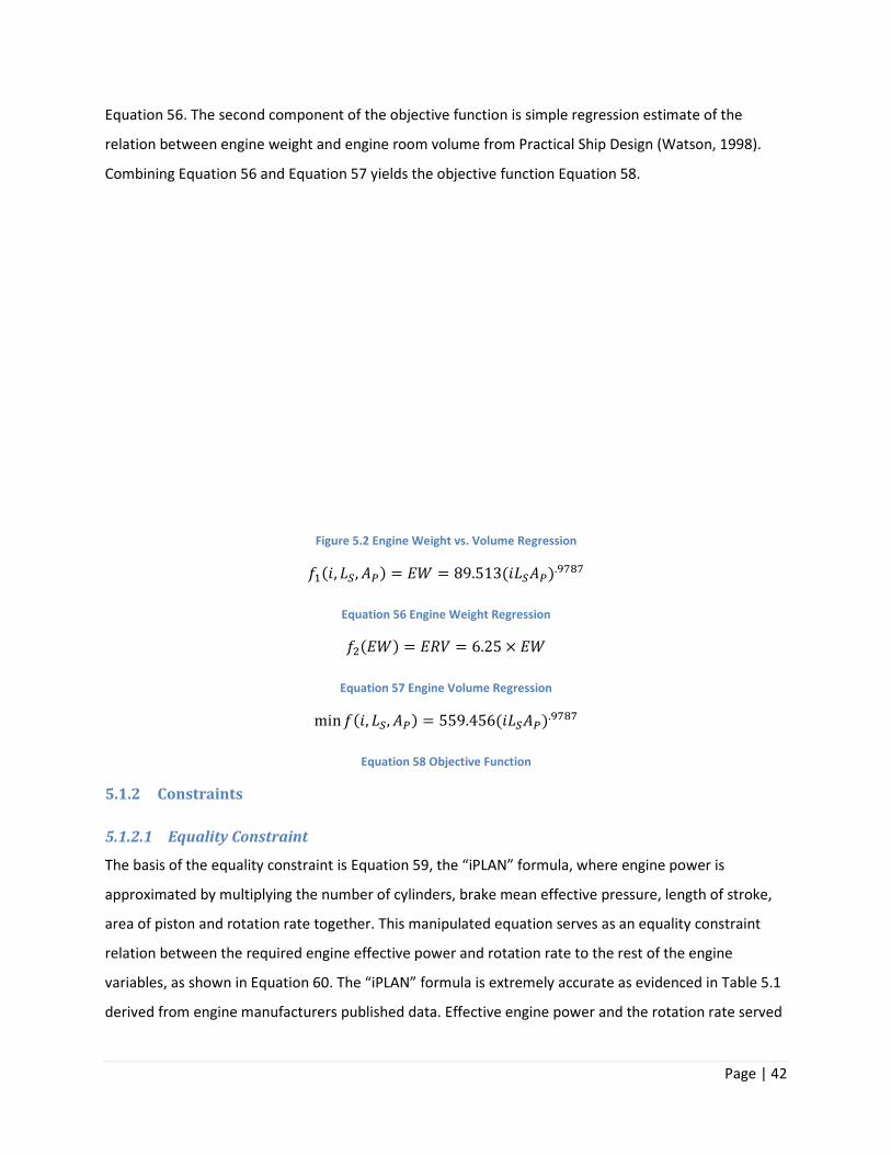
Equation 56. The second component of the objective function is simple regression estimate of the

relation between engine weight and engine room volume from Practical Ship Design

Combining Equation 56 and Equation

Figure

q�S

min

5.1.2 Constraints

5.1.2.1 Equality Constraint

The basis of the equality constraint is

approximated by multiplying the number of cylinders, brake mean effective pressure, length of stroke,

area of piston and rotation rate together.

relation between the required engine effective power and rotation r

variables, as shown in Equation 60.

derived from engine manufacturers published data. Effective engine pow

. The second component of the objective function is simple regression estimate of the

engine weight and engine room volume from Practical Ship Design (Watson, 1998)

Equation 57 yields the objective function Equation 58.

Figure 5.2 Engine Weight vs. Volume Regression

, �:, A�� y� � 89.513S�:A��."$*$

Equation 56 Engine Weight Regression

q�y�� y�D � 6.25 � y�

Equation 57 Engine Volume Regression

min qS, �:, A�� 559.456S�:A��."$*$

Equation 58 Objective Function

The basis of the equality constraint is Equation 59, the “iPLAN” formula, where engine power is

multiplying the number of cylinders, brake mean effective pressure, length of stroke,

area of piston and rotation rate together. This manipulated equation serves as an equality constraint

relation between the required engine effective power and rotation rate to the rest of the engine

. The “iPLAN” formula is extremely accurate as evidenced in

derived from engine manufacturers published data. Effective engine power and the rotation rate served

Page | 42

. The second component of the objective function is simple regression estimate of the

(Watson, 1998).

, the “iPLAN” formula, where engine power is

multiplying the number of cylinders, brake mean effective pressure, length of stroke,

anipulated equation serves as an equality constraint

ate to the rest of the engine

The “iPLAN” formula is extremely accurate as evidenced in Table 5.1

er and the rotation rate served

Page | 43

as parameters to be input from propeller optimization, while the number of cylinders, length of stroke,

area of piston and brake mean effective pressure acted as variables.

��, �, ��, ��, �� = �� = ��

Equation 59 “iPLAn” Forumula

ℎ�S, X, �:, A� , 5� = XT − SX�:A�5 = 0

Equation 60 Equality Constraint

Table 5.1 “iPLAN” Formula Accuracy

5.1.2.2 Inequality Constraints

The only discrete variable in the objective function was the number of cylinders. The optimizer was run

for each discrete value, with the lowest returned objective value of the set being returned. The largest

two-stroke marine diesel in the world has fourteen cylinders. The optimizer was allowed a range of 1-15.

G� � 1 − S ≤ 0

Equation 61 i Lower Bound

G� � S − 15 ≤ 0

Equation 62 I Upper Bound

The length of stroke for two-stroke marine diesels ranges from about 1.5-2.5 meters. The optimizer was

allowed a range of 1.5-2.5 meters.

Engine Rated Power [kW] iPLAN [kW] Δ

RT-flex35 6960 6973.20 0.19%

RT-flex40 9080 9092.72 0.14%

RT-flex48T 11640 11643.90 0.03%

RT-flex50 13960 13975.37 0.11%

RT-flex58T 18080 18051.87 -0.16%

RT-flex60C 21780 21757.10 -0.11%

RT-flex68 25040 25024.70 -0.06%

RT-flex82C 54240 54217.46 -0.04%

RT-flex82T 40680 40637.43 -0.10%

RT-flex84T 37800 37810.94 0.03%

RT-flex96C 80080 80105.49 0.03%

iPLAN Formula Accuracy

Page | 44

G� � 1.5 − �: ≤ 0

Equation 63 Ls Lower Bound

G# � �: − 2.5 ≤ 0

Equation 64 Ls Upper Bound

Piston area was calculated from bore size, which ranges from about 0.3-1 meter. The optimizer was

allowed a range of 0.25-1 meter. The reason for the strict upper limit on bore size is the manufacturing

process. The largest two-stroke marine diesels share a common cylinder frame for different sizes of

bores. The current largest engine has a bore of 0.96 meters, and it was not practical to go beyond that.

A� − } �� 2� ��

= 0

Equation 65 Piston Area

G) � 0.25 − �� ≤ 0

Equation 66 Bcyl Lower Bound

G, � �� − 1 ≤ 0

Equation 67 Bcyl Upper Bound

Brake mean effective pressure was constrained within the typical range found in both real engine data

and the NA 331 Coursepack (Parsons, 2007), 15-30 bar.

G$ � 1500000 − X ≤ 0

Equation 68 BMEP Lower Bound

G* � X − 3000000 ≤ 0

Equation 69 BMEP Upper Bound

5.1.3 Feasibility

The model was deemed feasible for two reasons. First, the objective and constraint functions are

continuous. Additionally, all functions are monotonic within the constraint boundaries, and these

boundaries contain the complete set of feasible real world engines used to construct the model.

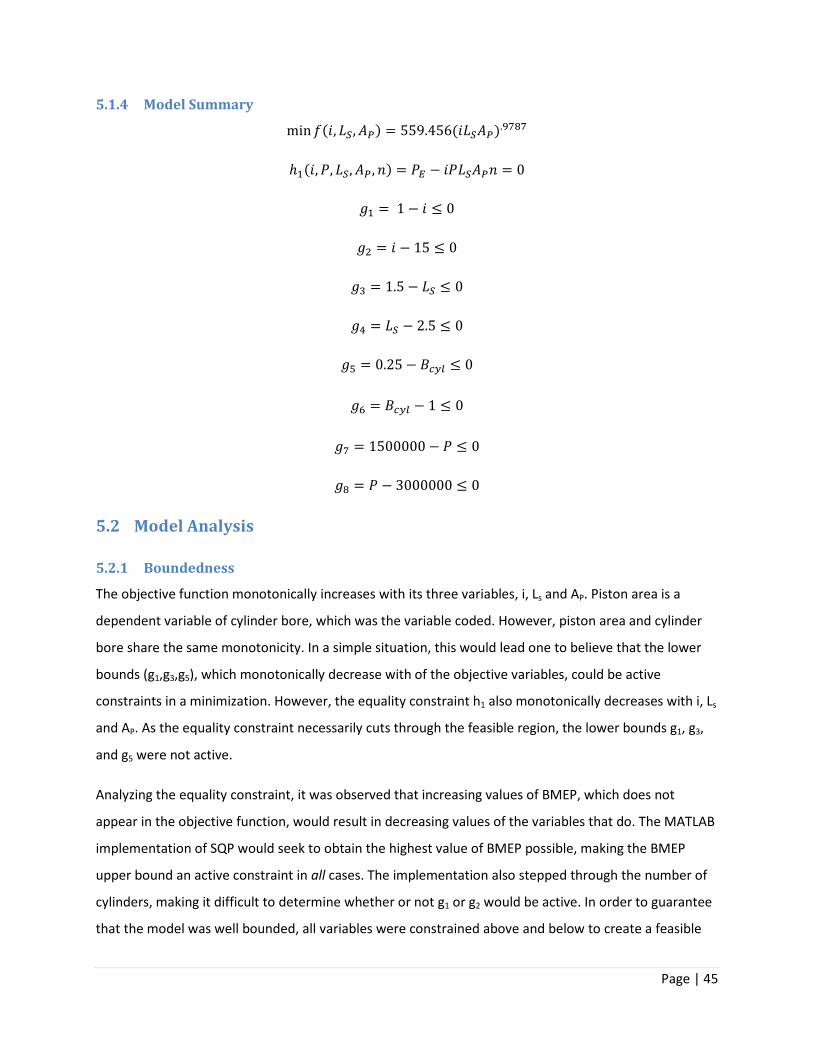
Page | 45

5.1.4 Model Summary

min qS, �:, A�� = 559.456S�:A��."$*$

ℎ�S, X, �:, A� , 5� = XT − SX�:A�5 = 0

G� = 1 − S ≤ 0

G� = S − 15 ≤ 0

G� = 1.5 − �: ≤ 0

G# = �: − 2.5 ≤ 0

G) = 0.25 − �� ≤ 0

G, = �� − 1 ≤ 0

G$ = 1500000 − X ≤ 0

G* = X − 3000000 ≤ 0

5.2 Model Analysis

5.2.1 Boundedness

The objective function monotonically increases with its three variables, i, Ls and AP. Piston area is a

dependent variable of cylinder bore, which was the variable coded. However, piston area and cylinder

bore share the same monotonicity. In a simple situation, this would lead one to believe that the lower

bounds (g1,g3,g5), which monotonically decrease with of the objective variables, could be active

constraints in a minimization. However, the equality constraint h1 also monotonically decreases with i, Ls

and AP. As the equality constraint necessarily cuts through the feasible region, the lower bounds g1, g3,

and g5 were not active.

Analyzing the equality constraint, it was observed that increasing values of BMEP, which does not

appear in the objective function, would result in decreasing values of the variables that do. The MATLAB

implementation of SQP would seek to obtain the highest value of BMEP possible, making the BMEP

upper bound an active constraint in all cases. The implementation also stepped through the number of

cylinders, making it difficult to determine whether or not g1 or g2 would be active. In order to guarantee

that the model was well bounded, all variables were constrained above and below to create a feasible

Page | 46

region in which real world engines exist. The first level monotonicity table is shown in Table 5.2.

Constraint activity for variables other than BMEP were determined from results.

Table 5.2 1st

Level Monotonicity Table


As predicted, the upper bound of BMEP was always an active constraint. The constraints g1, g3 and g5

were never active as described earlier. The constraint g2 was active only for high PE low BMEP situations,

which require the engine to be of larger geometric size. For the majority of low PE cases, either g4 or g6

were active. Based on this analysis, and the fact that not all independent variables were in the objective

function, it can be said that g2, g4 and g6 are semi-active constraints. An example is shown in Table 5.3,

where the test case is consistent with the other subsystems. The equality constraint h1, by definition

was always active, as was the iterated BMEP upper bound g8.

Active Constraints Pe=28651 [kW] n=0.85 [rps]

BMEP [Pa] g2 g4 g6

BMEP

[Pa] g2 g4 g6

3000000 2250000 X

2950000 2200000 X

2900000 2150000 X

2850000 2100000 X

2800000 2050000 X

2750000 2000000 X

2700000 X 1950000 X

2650000 1900000 X

2600000 1850000 X

2550000 X 1800000 X

2500000 X 1750000 X

2450000 X 1700000 X

2400000 X 1650000 X

2350000 X 1600000 X

2300000 X 1550000 X Table 5.3 Test Case Constraint Activity

f h1 g1 g2 g3 g4 g5 g6 g7 g8

i + - - +

Ls + - - +

Bcyl + - - +

P - - +

Monotonicity Table

Page | 47


5.3.1 Implementation

This model was developed to explore the tradeoff between fuel consumption and engine room volume.

This relationship cannot be demonstrated with a single optimum, but rather a Pareto front. The MATLAB

implementation of SQP, fmincon ,used for this model is a single objective minimization function

incapable of developing fronts. Using monotonicity and experience, it was determined that the upper

bound on BMEP would always be active. Due to the linear relationship between BMEP and SFC, BMEP

was used within the model, and results were converted to SFC or FC as a post process. To develop the

Pareto front, the upper bound on BMEP was iteratively stepped toward its lower bound, demonstrating

the range of fuel consumptions. If no feasible solution was found, none was recorded. In this fashion,

the Pareto front was generated to whatever level of accuracy was desired. It would have been possible

to treat BMEP as a parameter in this process, but it was left as a variable to verify that g8 was in fact

always active.

An additional complication was the discrete nature of the number of cylinders. One solution was to

convert i to a continuous variable, and then evaluate the bounding values once an optimum was found.

This method was discarded as the interaction effects between i and the other variables were hard to

distinguish along the Pareto front. Instead, i was treated as a parameter, with each discrete value being

tested every iteration through the BMEP bounds. The combination of variables leading to the lowest

objective value at each BMEP step was stored. This process is illustrated in Figure 5.3.

Figure 5.3 Pareto Front Process

5.3.2 Results

The Pareto front for the test case can be seen in Figure 5.3, with a table of results shown in Table 5.4.

The constraint activity for this case is described in the previous section. It is fair to say that the high

Lower BMEP Upper Bound

SQP for each i

Record Best Solution

Page | 48

BMEP solutions are more likely to be interior optima in terms of the other variables. This is the result of

the equality constraint satisfaction, where high BMEP reduces the other variables for the same effective

power. This is evidenced in Figure 5.4. A wide range of initial conditions were tried, but the resulting

Pareto front did not change.

Figure 5.4 Engine Subsystem Test Case Results

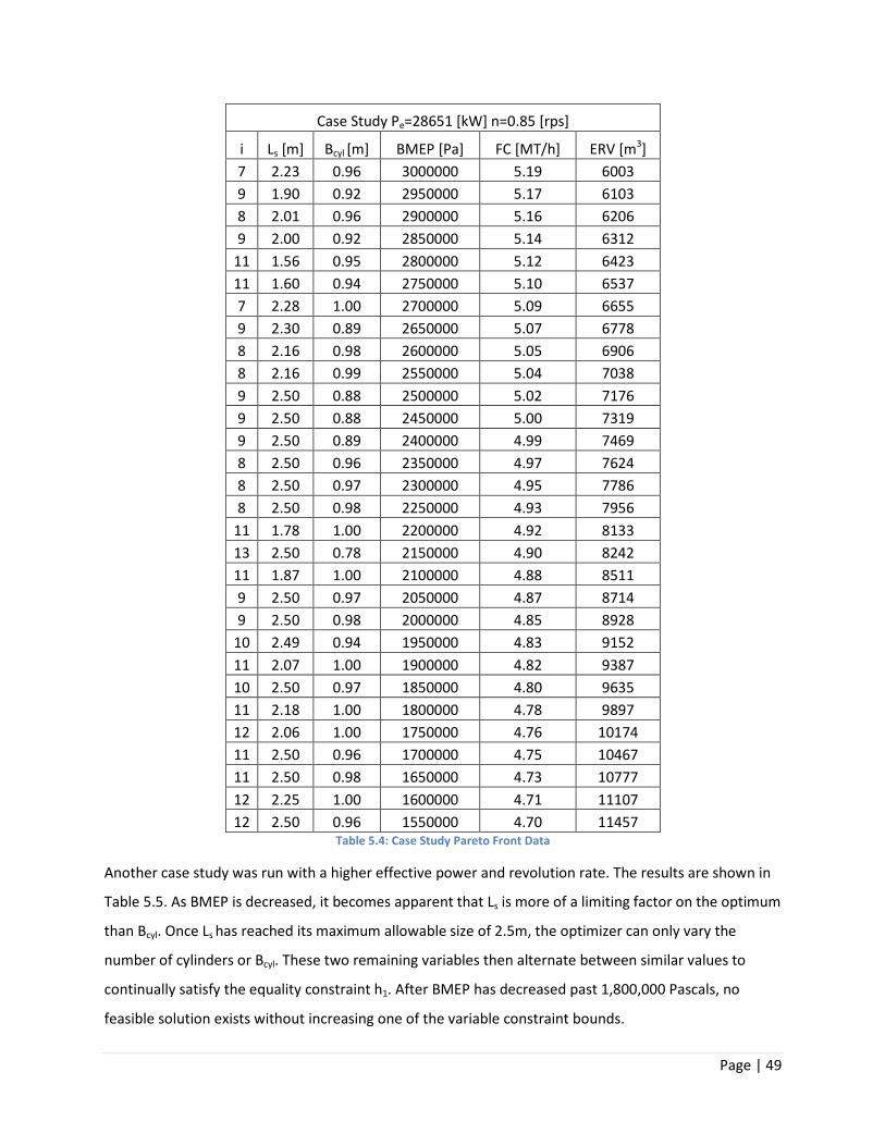
Page | 49

Case Study Pe=28651 [kW] n=0.85 [rps]

i Ls [m] Bcyl [m] BMEP [Pa] FC [MT/h] ERV [m3]

7 2.23 0.96 3000000 5.19 6003

9 1.90 0.92 2950000 5.17 6103

8 2.01 0.96 2900000 5.16 6206

9 2.00 0.92 2850000 5.14 6312

11 1.56 0.95 2800000 5.12 6423

11 1.60 0.94 2750000 5.10 6537

7 2.28 1.00 2700000 5.09 6655

9 2.30 0.89 2650000 5.07 6778

8 2.16 0.98 2600000 5.05 6906

8 2.16 0.99 2550000 5.04 7038

9 2.50 0.88 2500000 5.02 7176

9 2.50 0.88 2450000 5.00 7319

9 2.50 0.89 2400000 4.99 7469

8 2.50 0.96 2350000 4.97 7624

8 2.50 0.97 2300000 4.95 7786

8 2.50 0.98 2250000 4.93 7956

11 1.78 1.00 2200000 4.92 8133

13 2.50 0.78 2150000 4.90 8242

11 1.87 1.00 2100000 4.88 8511

9 2.50 0.97 2050000 4.87 8714

9 2.50 0.98 2000000 4.85 8928

10 2.49 0.94 1950000 4.83 9152

11 2.07 1.00 1900000 4.82 9387

10 2.50 0.97 1850000 4.80 9635

11 2.18 1.00 1800000 4.78 9897

12 2.06 1.00 1750000 4.76 10174

11 2.50 0.96 1700000 4.75 10467

11 2.50 0.98 1650000 4.73 10777

12 2.25 1.00 1600000 4.71 11107

12 2.50 0.96 1550000 4.70 11457 Table 5.4: Case Study Pareto Front Data

Another case study was run with a higher effective power and revolution rate. The results are shown in

Table 5.5. As BMEP is decreased, it becomes apparent that Ls is more of a limiting factor on the optimum

than Bcyl. Once Ls has reached its maximum allowable size of 2.5m, the optimizer can only vary the

number of cylinders or Bcyl. These two remaining variables then alternate between similar values to

continually satisfy the equality constraint h1. After BMEP has decreased past 1,800,000 Pascals, no

feasible solution exists without increasing one of the variable constraint bounds.

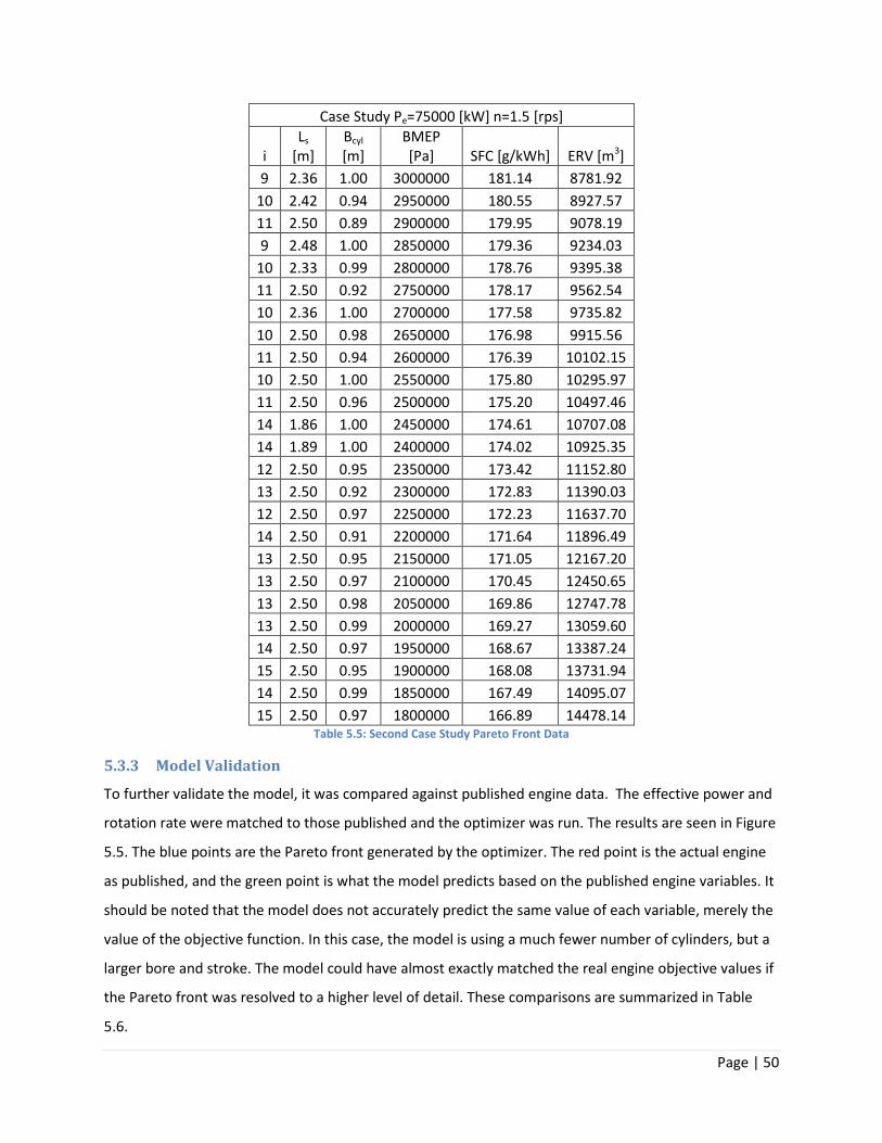
Page | 50

Case Study Pe=75000 [kW] n=1.5 [rps]

i

Ls

[m]

Bcyl

[m]

BMEP

[Pa] SFC [g/kWh] ERV [m3]

9 2.36 1.00 3000000 181.14 8781.92

10 2.42 0.94 2950000 180.55 8927.57

11 2.50 0.89 2900000 179.95 9078.19

9 2.48 1.00 2850000 179.36 9234.03

10 2.33 0.99 2800000 178.76 9395.38

11 2.50 0.92 2750000 178.17 9562.54

10 2.36 1.00 2700000 177.58 9735.82

10 2.50 0.98 2650000 176.98 9915.56

11 2.50 0.94 2600000 176.39 10102.15

10 2.50 1.00 2550000 175.80 10295.97

11 2.50 0.96 2500000 175.20 10497.46

14 1.86 1.00 2450000 174.61 10707.08

14 1.89 1.00 2400000 174.02 10925.35

12 2.50 0.95 2350000 173.42 11152.80

13 2.50 0.92 2300000 172.83 11390.03

12 2.50 0.97 2250000 172.23 11637.70

14 2.50 0.91 2200000 171.64 11896.49

13 2.50 0.95 2150000 171.05 12167.20

13 2.50 0.97 2100000 170.45 12450.65

13 2.50 0.98 2050000 169.86 12747.78

13 2.50 0.99 2000000 169.27 13059.60

14 2.50 0.97 1950000 168.67 13387.24

15 2.50 0.95 1900000 168.08 13731.94

14 2.50 0.99 1850000 167.49 14095.07

15 2.50 0.97 1800000 166.89 14478.14 Table 5.5: Second Case Study Pareto Front Data

5.3.3 Model Validation

To further validate the model, it was compared against published engine data. The effective power and

rotation rate were matched to those published and the optimizer was run. The results are seen in Figure

5.5. The blue points are the Pareto front generated by the optimizer. The red point is the actual engine

as published, and the green point is what the model predicts based on the published engine variables. It

should be noted that the model does not accurately predict the same value of each variable, merely the

value of the objective function. In this case, the model is using a much fewer number of cylinders, but a

larger bore and stroke. The model could have almost exactly matched the real engine objective values if

the Pareto front was resolved to a higher level of detail. These comparisons are summarized in Table

5.6.

Page | 51

Figure 5.5 Engine Subsystem Model Validation

Model Validation

i Ls [m] Bcyl BMEP [bar] SFC [g/kWh] EW [MT] ERV* [m3]

Real Engine 9 2.25 0.6 20 171 480 3000

Model Predicted Real

Engine 9 2.25 0.6 20 169.26 493 3086

Nearest Pareto point to

Real Engine 3 2.5 0.97 20.5 169.86 483 3016

* This is EWx6.25 in all cases Table 5.6 Model Validation Data

Not all validation runs were as exact as this case, as shown in Figure 5.6 for other engines in the same

series. It should be noted that the gaps in the Pareto fronts are due to discrete cylinder number jumps.

As a test, the geometric constraints were slightly relaxed and the resulting fronts did not have gaps. The

model validation shows that the optimizer is not capable of predicting a set of engine variables, but can

accurately predict engine weight and fuel consumption. The engine room volume prediction is only as

good as Equation 57, for which real world validation data is difficult to obtain.

Page | 52

Figure 5.6 Multiple Engine Subsystem Model Validation

5.4 Parametric Studies

Figure 5.7 shows the resulting Pareto fronts when effective power is lowered from 100,000 KW to only

10,000 KW. What is interesting about this case is that with high engine powers, the lower range of SFC is

not available, as the upper bounds on Bcyl, i and or Ls are active such that BMEP cannot be lowered any

further. At some point, around 80,0000 KW the complete range of SFC is available. Obviously, lower

power engines require less ERV as is evidenced.

Page | 53

Figure 5.7 Variation of Effective Power, Constant rps (1.5)

Figure 5.8 shows the same data, except that FC is plotted on the x-axis. Fuel Consumption is merely the

SFC multiplied by the effective power. What is interesting about this plot is that an 80,000 KW engine

could actually take up more volume than a 100,000 KW engine. The explanation is that with the higher

engine powers the lower range of BMEP is not available, requiring them to utilize the upper end of the

BMEP options and subsequently less volume. The largest 80,000 KW engine has a lower pressure

capability, requiring more volume. This interesting feature is a symptom of the model, rather than the

real world behavior. If the BMEP step in the implementation loop was smaller it would be shown that

the larger engines share the same maximum ERV. This is because the maximum ERV is defined by upper

engine variable constraint bounds. So long as the lowest feasible BMEP is greater than its lower bound,

the maximum ERV of every engine would be the same. The course BMEP step prevents this from

showing in Figure 5.8. Also note that this feature is also visible in Figure 5.7. Please note that the (0,0)

point in Figure 5.8 is not part of the data set, merely a consequence of bad coding.

Page | 54

Figure 5.8 Variation of Effective Power, Constant rps (1.5)

Figure 5.9 shows an opposite trend to the preceding two figures. As the revolution rate decreases, the

ERV increases. After the rps decreases enough, the lower bound on BMEP is no longer active, and the

equality constraint takes over. At this point, the minimum fuel consumption gets steadily higher as well.

The general trend shown by these two parametric studies is that the minimum ERV is obtained by the

higher revolution rates and higher fuel consumptions. Additionally, and obviously, lower power engines

take up less volume. The second study shows that a higher rps can decrease fuel consumption and

engine room volume. If the engine subsystem were considered alone, the optimal solution set would

have higher revolution rates.

Page | 55

Figure 5.9 Decreasing rps, Constant Effective Power (75,000 kW)

5.5 Results Discussion

The design implications of the engine subsystem results are as follows. First, the smallest engine room

volumes will be achieved with the highest fuel consumption, illustrating the tradeoff this model was

designed to explore. Secondly, higher power engines do not offer a designer as much freedom along the

Pareto front as lower power engines. As engine power is increased, the physical constraint boundaries

limit the range of feasible solutions. Lastly, a higher revolution rate decreases both engine room volume

and fuel consumption. Typical containerships have direct drive systems, meaning that the revolution

rate of the propeller and engine are the same. Utilizing the engine subsystem results alone would imply

that a faster revolution rate would result in a better global Pareto front. Unfortunately, propellers

perform better at slower speeds as shown in the preceding propeller subsystem discussion. The hull

form parameters affect propeller performance, which indirectly will influence the engine subsystem as

well.

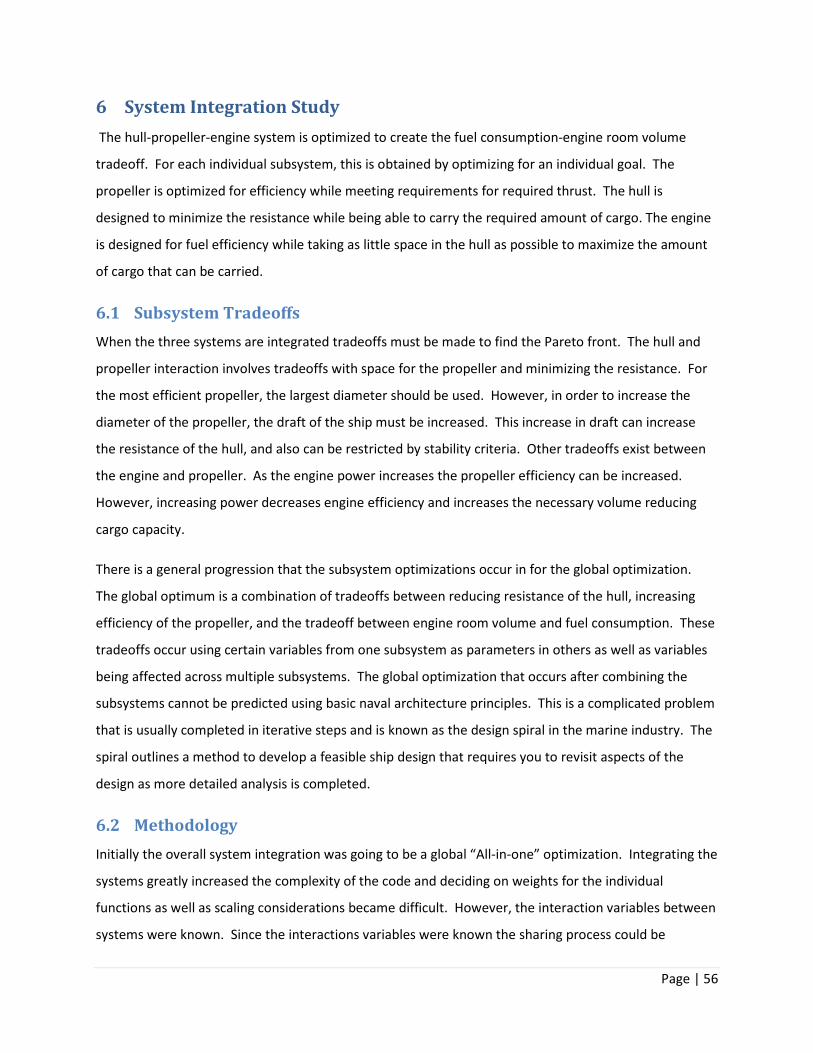
Page | 56

6 System Integration Study

The hull-propeller-engine system is optimized to create the fuel consumption-engine room volume

tradeoff. For each individual subsystem, this is obtained by optimizing for an individual goal. The

propeller is optimized for efficiency while meeting requirements for required thrust. The hull is

designed to minimize the resistance while being able to carry the required amount of cargo. The engine

is designed for fuel efficiency while taking as little space in the hull as possible to maximize the amount

of cargo that can be carried.

6.1 Subsystem Tradeoffs

When the three systems are integrated tradeoffs must be made to find the Pareto front. The hull and

propeller interaction involves tradeoffs with space for the propeller and minimizing the resistance. For

the most efficient propeller, the largest diameter should be used. However, in order to increase the

diameter of the propeller, the draft of the ship must be increased. This increase in draft can increase

the resistance of the hull, and also can be restricted by stability criteria. Other tradeoffs exist between

the engine and propeller. As the engine power increases the propeller efficiency can be increased.

However, increasing power decreases engine efficiency and increases the necessary volume reducing

cargo capacity.

There is a general progression that the subsystem optimizations occur in for the global optimization.

The global optimum is a combination of tradeoffs between reducing resistance of the hull, increasing

efficiency of the propeller, and the tradeoff between engine room volume and fuel consumption. These

tradeoffs occur using certain variables from one subsystem as parameters in others as well as variables

being affected across multiple subsystems. The global optimization that occurs after combining the

subsystems cannot be predicted using basic naval architecture principles. This is a complicated problem

that is usually completed in iterative steps and is known as the design spiral in the marine industry. The

spiral outlines a method to develop a feasible ship design that requires you to revisit aspects of the

design as more detailed analysis is completed.

6.2 Methodology

Initially the overall system integration was going to be a global “All-in-one” optimization. Integrating the

systems greatly increased the complexity of the code and deciding on weights for the individual

functions as well as scaling considerations became difficult. However, the interaction variables between

systems were known. Since the interactions variables were known the sharing process could be

Page | 57

simplified from the “All in One” approach.. Instead of having variables shared between systems, vectors

of decision variables of one subsystem became parameters in the remaining subsystems.

Knowing the interactions a priori allowed the system optimization to be handled in a sequential manner.

The main interaction that needed to be examined was the relationship between hull draft, hull

resistance, and propeller efficiency. Vectors of resistances and corresponding drafts from the hull

optimization were used as parameters in the propeller optimization subsystem. The propeller

optimization algorithm then output vectors of required engine power, and required engine revolution

rates. To approach the problem, the case study ship of 75,000 m3 and 18 knots was examined.

The optimum propeller efficiency was nearly always at the largest draft possible, while the lowest

resistance may be at a smaller draft. That there was an interaction was known before running the

optimization. In an “All in One” it would be unclear how much weight should be put on each subsystem..

This would be more complicated because the weighting would assume that the integrated system

behaves in the same fashion for different inputs, which was not always the case as shown with varying

constraint activity in the subsystems.

The engine subsystem creates a Pareto Front for each of the input engine rps and required power when

the hull and propeller systems are finished with iterating the range of input drafts. The Pareto front

examines the different tradeoffs between fuel consumption and engine room volume. By examining the

Pareto Front for the entire system design selections can be made. Due to lack of further information the

point closest to utopia was chosen. If data was known on fuel prices or cargo rates further tradeoffs

could be examined. For example, if cargo prices are high, the designer may be willing to give up fuel

efficiency for more cargo volume. Figure 6.1 visually shows the sequential optimization process.

Figure

6.3 System Optimization Results

The results of the integrated system optimization are presented similarly to the engine subsystem. For

this study, the same objective that the engine subsystem had

A tradeoff of fuel consumption to engine

subsystem optimization was calculated for was considered for the integrated system. The ship speed

was 18 knots and the volume was 75,000 cubic meters. Feasible solutions were generated and a Pareto

front was formed. Figure 6.2 shows both the feasible solutions as well as the Pareto front. From the

Pareto front, the group selected a design using the n

utopian point is the point where both objectives are thei

never be reached, but the selection process uses the distance from this point to select the final design.

Figure 6.2 shows the selected design as the green dot. This point on the lef

the shortest distance from the utopian because the scaling of the figure is warped. After rescaling the

figure, which can be seen on the right, the selected design looks closer to the utopian. Using

engineering judgment, it was determined that the selected design would be close to what an actual

engineer would pick manually.

Figure 6.1 System Optimization Sequence

System Optimization Results

egrated system optimization are presented similarly to the engine subsystem. For

ve that the engine subsystem had was also the global optimization objective.

A tradeoff of fuel consumption to engine room volume was evaluated. The case study that each



shows both the feasible solutions as well as the Pareto front. From the

up selected a design using the nearest to the Utopian selection process. The

utopian point is the point where both objectives are their smallest respective values. This point can


shows the selected design as the green dot. This point on the left figure does not look like it is



it was determined that the selected design would be close to what an actual

Page | 58

egrated system optimization are presented similarly to the engine subsystem. For

was also the global optimization objective.

The case study that each



shows both the feasible solutions as well as the Pareto front. From the

earest to the Utopian selection process. The

r smallest respective values. This point can


t figure does not look like it is



it was determined that the selected design would be close to what an actual

Page | 59

Figure 6.2 System Integration Pareto Front

To determine if the shape of the Pareto front could ever change, the ship speed and volume were

changed and the integrated system optimization was completed again. The new speed and volume was

25 knots and 40,000 cubic meters, respectively. The Pareto front and selected design for this case is

provided in Figure 6.3. It can be seen that the shape of the Pareto front is similar. Also, the selected

design was in the same area for both cases. The distinct blue bands on the left of Figure 6.1 and Figure

6.2 are the individual Pareto fronts for the varying drafts. The red band is the overall Pareto front. By

decreasing the increment of the input draft vector, this Pareto front could be made to look nearly

continuous.

Figure 6.3 System Integration Validation Pareto Front

6.4 Comparison to Subsystem Optimization

The results of the integrated system optimization were then compared to the results of optimizing the

subsystems individually. Table 6.1 displays the tradeoffs made when the system is integrated compared

Page | 60

to the individually optimized subsystems. The table shows that although the required thrust due to

resistance and propeller efficiency are less than optimal, a better point between engine room volume

and fuel efficiency can be found.

For the required volume and speed used, the optimal draft is near the limits of the optimization model

used. This gives results for the hull form optimization and propeller optimization that are close in final

outputs for engine room volume and fuel consumption. The major tradeoff became losing fuel

efficiency for a higher BMEP, which allows for smaller engines capable of the same power. The overall

system optimization results in a 28.9% decrease in engine room volume with only a 6.1% increase in fuel

consumption. The integrated system uses a draft of 14.5, compared to 14.64 meters for the hull

subsystem optimization and 15 meters for the propeller. The required thrust from the hull subsystem

optimization is nearly constant in the integrated system, and the propeller efficiency is decreased only

slightly. These results imply that for this hull the engine or propeller optimum main parameters would

be acceptable, the real tradeoff is within the engine room with BMEP. This result may vary with different

input parameters.

Solution Comparison ∇=75,000 m3 Vs=18 knots

Hull Form Propeller Int. System

Tm [m] 14.64 15 14.5

RT [kN] 1036.5 1036.7 1036.6

ηo 0.723 0.723 0.721

PE [kW] 28651 28491 28720

BMEP [bar] 21.5 21.5 30

n [rps] 0.85 0.8 0.86

Min FC [MT/h] 4.69 4.67 4.69

ERV [m3] 6003 6248 3512

Selected FC [MT/h] 4.9 4.9 5.2

ERV [m3] 8318 8656 5912 Table 6.1 Subsystem Optimization Comparison

6.5 Integrated System Parametric Study

Several parameter values were entered into the combined system to find how they affected the design.

The parameters that were examined were hull resistance, propeller rps, propeller efficiency, draft, and

effective power. For each of the parameters examined, the minimum engine room volumes and fuel

consumptions were found over the reasonable ranges of parameter values. By completing the

Page | 61

parametric study it can be observed how changing aspects of the hull or propeller will influence the

optimal design.

The first parameter examined was the hull resistance. Figure 6.4 shows the relationship between engine

room volume and fuel consumption when compared to different ship hull resistances. For the higher

range of increasing resistance the engine room volume varies little. The fuel consumption on the other

hand increases more drastically with increasing resistance. This implies that changing resistance could

improve fuel efficiency greatly, without having much impact on engine room volume. On the low range,

this relationship does not hold. The near vertical line on the left of the figures shows where there are a

broader range of options available. This corresponds to the steepest part of the Pareto front shown in

Figure 6.2, and near the selected design.

Figure 6.4: Engine Room Volume and Fuel Consumption vs. Resistance

The propeller revolutions per second also influenced the engine room volume and fuel consumption of

the combined system. As when the resistance was increased for higher ranges, changing the propeller

rps had a larger affect on the fuel consumption than engine room volume. In the lower range, this

relationship does not hold. This can be seen in Figure 6.5.

Page | 62

Figure 6.5: Engine Room Volume and Fuel Consumption vs. Propeller RPS

Figure 6.6 shows an opposite trend to the proceeding two relationships. Higher drafts generally result in

larger and more efficient propellers, yet slower revolution rates. This can be seen as the explosion of

engine room volume on the right of the figure. These slower engines generally had lower fuel

consumption because less overall power was being demanded. The integrated system optimum

occurred in the higher draft range, just before the engine room volume explodes.

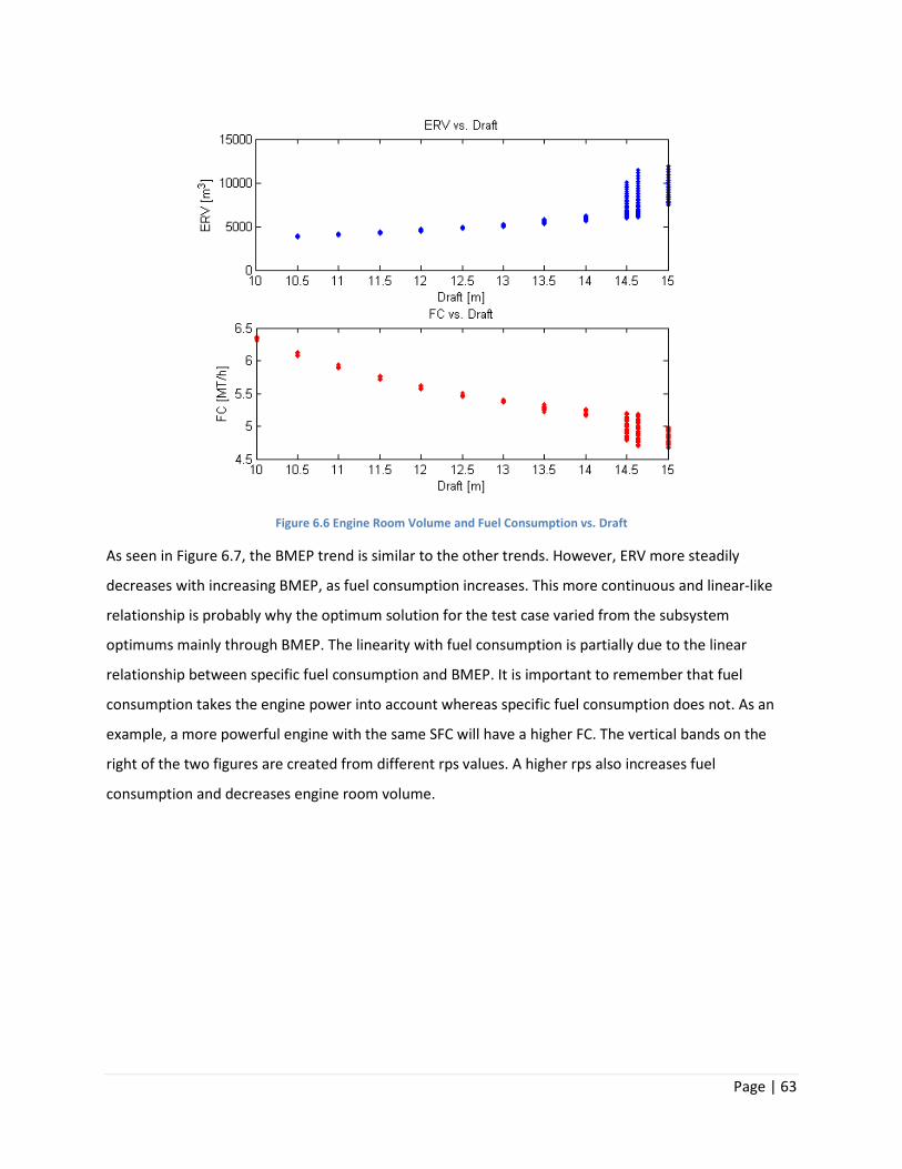
Page | 63

Figure 6.6 Engine Room Volume and Fuel Consumption vs. Draft

As seen in Figure 6.7, the BMEP trend is similar to the other trends. However, ERV more steadily

decreases with increasing BMEP, as fuel consumption increases. This more continuous and linear-like

relationship is probably why the optimum solution for the test case varied from the subsystem

optimums mainly through BMEP. The linearity with fuel consumption is partially due to the linear

relationship between specific fuel consumption and BMEP. It is important to remember that fuel

consumption takes the engine power into account whereas specific fuel consumption does not. As an

example, a more powerful engine with the same SFC will have a higher FC. The vertical bands on the

right of the two figures are created from different rps values. A higher rps also increases fuel

consumption and decreases engine room volume.

Page | 64

Figure 6.7 Engine Room Volume and Fuel Consumption vs. BMEP

The remainder of the parametric studies show trends similar to the ones presented above. They do not

lend any more insight into the model, but are available upon request.

6.6 Conclusions

The optimization study completed for the integrated system provides valuable insights and methods of

improving ship design during the initial design stages. A process that is typically completed individually

with little communication between systems can now be completed as one while incorporating the

known design tradeoffs. The results show that the interactions between the resistance and propeller

subsystems can be predicted. The combination of all three subsystems is the most interesting and

challenging aspect of this optimization study. Instead of simply choosing an engine from a catalog that

meets power requirements, a more in depth analysis can reveal other alternatives that allow the

designer to choose a more optimal design. Although this optimization study provided valuable insights,

it is important to note that this is a simple analysis based on regression analysis that does not apply to

all ship designs. Further work should be completed in an attempt to fully optimize the propulsion

system on more types of ships as well as improving on certain assumptions made for simplicity

purposes.

Page | 65

7 Bibliography

Bernitsas, M. M., & Ray, D. (1982). Optimal Revolution B-Series Propellers. Ann Arbor: The University of

Michigan Department of Naval Architecture and Marine Engineering.

Bernitsas, M. M., Ray, D., & Kinley, P. (1981). KT, KQ and Efficiency Curves for the Waneningen B-Series

Propellers. Ann Arbor: University of Michigan Department of Naval Architecture and Marine

Engineering.

Holtrop, J. (1984). A Statistical Re-Analysis of Resistance and Propulsion Data. International Shipbuilding

Progress , 272-276.

Holtrop, J., & Mennen, G. (1982). An Approximate Power Prediction Method. International Shipbuilding

Progress , 166-170.

Parsons, M. (2007). Informal Course Notes for NA331 Marine Engineering I. Ann Arbor: University of

Michigan Department of Naval Architecture and Marine Engineering.

Parsons, M. (2007). Informal Ship Design Course Notes for NA470 Foundations of Ship Design and NA570

Advanced Marine Design. University of Michigan Department of Naval Architecture and Marine

Engineering.

Van Manen, J., & Van Oossanen, P. (1988). Propulsion. In E. V. Lewis, Principles of Naval Architecture

Volume II (pp. 127-240). Jersey City: The Society of Naval Architects and Marine Engineers.

Wärtsilä. (n.d.). Wärtsilä RT-flex96C and RTA96C. Retrieved February 2010, from Wärtsilä:

http://www.wartsila.com/,en,productsservices,productdetail,product,106F8B1D-FFFA-400A-9F3A-

7C4B5FBF7A47,5B676C68-5794-4765-AB44-4077CD1BF36F,,8001.htm

Watson, D. (1998). Practical Ship Design. Oxford: Elsevier Science Ltd.

Page | 66

Appendix A Hull Code

1. Hull Optimization Code

clear all

global g Vs Cwp Cm xcb atr Cstern Sapp Abt hb vol Cp

options = optimset('Display','iter','MaxFunEvals',1000);

% SHIP VARIABLES Tm = 8; % draft at midship in [m] lwl = 200; % length of waterline [m] bwl = 25; % breadth of waterline [m] Cb = 0.3; D = 14;

%PARAMETERS %velocity Vskn = 18; Vs = Vskn / 3.6 * 1.852; % ship speed in [m/s]

%optimization A=[]; b=[]; Aeq=[]; beq=[]; lb=[0,0,0,0,0]; ub=[20,800,100,1,50];

[Rtopt,Rt,exitflag,ouput] =

fmincon('resistance',[Tm,lwl,bwl,Cb,D],A,b,Aeq,beq,lb,ub,'constraints',option

s)

2. Hull Objective Function

% Function holtrop - calculate ship total resistance using holtrop-mennen

systematic series % % Valid ship dimensions and valid main paramenters for the use of this method

can be found in % literature mentioned below. % Version 0.01 % % This function was uploaded to the Scilab contribution page and is freely

available % from http:%www.scilab.org/contrib/index_contrib.php?page=download.php % You are free to use, redistribute and modify this function, as long as the

author % and source are mentioned. The author won't guarantee or take responsability

for any of the % results given by this function, nor give any support.

Page | 67

% % all formulas and nomenclature are taken from following articles: % 1. Holtrop, J. & Mennen, G.: "An Approximate Power Prediction Method" % International Shipbuilding Progress vol. 329, pp166-170, 1982 % 2. Holtrop, J.: "A Statistical Re-Analysis of Resistance and Propulsion

Data" % International Shipbuilding Progress vol. 353, pp272-276, 1984 % % output parameters % Rt: list, total ship resistance in [kN] (if rho is given in tons/m^3), else

in [N].

function [Rt] = resistance(x)


%CONSTANTS (gravitation, density and viscosity) if not existant g=9.81; % g in [m/s^2] rho=1.025; % salt water density in tons/m^3 nu=1.19e-6; % kin. visc. in [m^2/s]

% SHIP VARIABLES Tm = x(1); % draft at midship in [m] lwl = x(2); % length of waterline [m] bwl = x(3); % breadth of waterline [m] Cb = x(4);

%SHIP PARAMETERS %velocity %Vskn = 25; %Vs = Vskn / 3.6 * 1.852; % ship speed in [m/s] % waterplane area coefficient Cwp=0.75; % Mid section coeff. Cm = 0.98; % longitudinal center of buoyancy [m] from midship section (+fwd, -aft) xcb = -4.141 ; % submerged area of transom [m^2] atr = 16; % Cstern: % Pram with gondola -25 % V-shaped sections -10 % Normal section shape 0 % U-shaped sections % with Hogner stern 10 Cstern = 10; % Sapp is area of appendages Sapp = 50; % Abt is transversal area of bulb at Fpp in [m^2] Abt = 20; % hb is center of area of Abt in [m] from keelline hb = 4;

%SUBSET CALCULATIONS vol = Cb*lwl*bwl*Tm; % volume of ship in [m^3].

Page | 68

sw = lwl.*(2.*Tm+bwl).*sqrt(Cm).*(0.453+0.4425*Cb-0.2862.*Cm-

0.003467.*(bwl./Tm)+0.3696.*Cwp)+2.38.*(Abt./Cb); % wetted surface in [m^2] Cp = vol./(Cm.*bwl.*Tm.*lwl); % prismatic coeff. ref. Lwl according to

Holtrop c14 = 1+0.011*Cstern; ams = Cm.*bwl.*Tm;

% resistance components with same nomenclatre as Holtrop-Mennen 82 & 84 % "an approximate power prediction method"

% lcb according to Holtrop lcb = 100 .* xcb ./ lwl; % Lr acc. Holtrop Lr = lwl .* (-Cp + 1 + (0.06.*Cp.*lcb)./(4.*Cp -1)); % calculate angle of entrance if not known ie = 1 + 89.*exp(-((lwl./bwl).^0.80856).*((1-Cwp).^0.30484).*((1-Cp-

0.0225.*lcb).^0.6367).*... ((Lr./bwl).^0.34574).*((100.*vol./(lwl.^3)).^0.16302)); % dummy form factor of appendages if not found k2 = 0.5; % calculate coefficients if bwl/lwl < 0.11 c7 = 0.229577.*(bwl./lwl).^0.33333; elseif (bwl/lwl >= 0.11) && (bwl/lwl < 0.25) c7 = bwl./lwl; else c7 = 0.5 - 0.0625.*lwl./bwl; end % calculate c16 if Cp < 0.8 c16 = 8.07981 * Cp - 13.8673 * Cp^2 + 6.984388 * Cp^3; else c16 = 1.73014 - 0.7067 * Cp; end % c15 if (lwl^3 / vol) < 512 c15 = -1.69385; elseif (lwl^3 / vol) >= 1726.91 c15 = 0; else c15 = -1.69385 + (lwl/(vol^(1/3)) - 8) / 2.36; end % calculate c2 and c3 c3 = 0.56 * (Abt^1.5) / (bwl*Tm*(0.31*(Abt)^0.5 + Tm - hb)); c2 = exp(-1.89*(c3)^0.5); % calculate lambda if lwl/bwl < 12 lambda = 1.446 * Cp - (0.03 * lwl / bwl); else lambda = 1.446 * Cp - 0.36; end

if Tm/lwl > 0.04 c4 = 0.04; else c4 = Tm/lwl;

Page | 69

end % form factor calculation k1 = (0.487118 *

c14).*((bwl./lwl).^1.06806).*((Tm./lwl).^0.46106).*((lwl./Lr).^0.121563).*... (((lwl.^3)./vol).^0.36486).*((1-Cp).^(-0.604247))+0.93-1; % other factors m1 = 0.0140407 * lwl./Tm -1.75254 .* (vol.^(1/3))./lwl - 4.79323 .* bwl./lwl

- c16; m3 = -7.2035.*((bwl./lwl).^0.326869).*((Tm./bwl).^0.605375); c1 = 2223105*(c7.^3.78613).*((Tm./bwl).^1.07961).*((90-ie).^(-1.37565)); c5 = 1 - (0.8 .* atr ./ ams); c17 = 6919.3.* (Cm.^(-1.3346)) .* ((vol./(lwl^3)).^2.00977) .* ((lwl./bwl -

2).^1.40692); m404 = c15 .* (0.4.*exp(-0.034.*(0.4.^(-3.29)))); m4055 = c15 .* (0.4.*exp(-0.034.*(0.55.^(-3.29)))); % ship-model correlation factor Ca = 0.006 .* ((lwl + 100).^(-0.16)) - 0.00205 +

0.003.*((lwl./7.5).^0.5).*Cb.^4 .*c2.*(0.04-c4); % calculate Holtrop-Mennen calm water resistance % calculate Rf Rn=Vs .* lwl ./ nu; cf= 0.075 ./ (log10(Rn)-2).^2; Rf = 1/2 .* rho .* Vs^2 .* sw .* cf; % calculate velocity dependant coefficients for Rw Fn = Vs./(lwl.*g).^0.5; m4 = c15 .* (0.4.*exp(-0.034.*(Fn.^(-3.29)))); % calculate wave resistance Rw_a (for Fn < 0.4) Rw_a = c1 .* c2 .* c5 .* vol .* rho .* g .* exp(m1 .* (Fn.^(-0.9)) + m4... .* cos((lambda .* (Fn.^(-2))))); % for Fn==0.4 Rw_a04 = c1 .* c2 .* c5 .* vol .* rho .* g .* exp(m1 .* (0.4.^(-0.9)) +

m404... .* cos((lambda .* (0.4.^(-2))))); % if Fn > 0.55 Rw_b Rw_b = c17 .* c2 .* c5 .* vol .* rho .* g .* exp(m3 .* (Fn.^(-0.9)) + m4... .* cos((lambda .* (Fn.^(-2))))); % for Fn ==0.55 Rw_b055 = c17 .* c2 .* c5 .* vol .* rho .* g .* exp(m3 .* (0.55.^(-0.9)) +

m4055... .* cos((lambda .* (0.55.^(-2))))); if Fn < 0.4 Rw = Rw_a; elseif Fn > 0.55 Rw = Rw_b; else % interpolation formula for values between 0.4 and 0.55 Rw = Rw_a04 + (10.*Fn - 4).*(Rw_b055 - Rw_a04)./1.5; end % calculate resistance due to presence of bulbous bow near water surface if Abt > 0 pb = 0.56 .* (Abt.^0.5) ./ (Tm - 1.5.*hb); Fni = Vs ./ (g.*(Tm - hb - 0.25.*(Abt).^0.5) + 0.15.*Vs).^0.5; Rb = 0.11 .* exp(-3.*pb.^(-2)) .* Fni^3 .* Abt.^1.5 .* rho .* g ./ (1 +

Fni.^2); else Rb = 0; end

Page | 70

if atr > 0 FnT = Vs / (2*g*atr / (bwl + bwl*Cwp))^0.5; else FnT = 0; end % calculate c6 if FnT < 5 c6 = 0.2*(1-0.2*FnT); else c6 = 0; end Rtr = 0.5 .* rho .* Vs.^2 .* atr .* c6; % calculate model-ship correlation resistance Ra = 0.5 .* rho .* Vs.^2 .* sw .* Ca; % calculate appendage resistance Rapp = (0.5 * rho * Vs * (1 + k2).*Sapp) .* cf ; % calculate total calm water resistance Rt = Rf.*(1 + k1) + Rapp + Rw + Rb + Rtr + Ra;

%endfunction

3. Hull Constraint Function

function [cong,conh] = constraints(x)


%stability constraint

Cvp = x(4)/Cwp; KB = x(1)*(Cwp/(x(4)+Cwp)); KG = 0.7*x(5); Ci = 0.0937*Cp-0.0122; It = Ci*x(2)*x(3)^3; BM = It/vol; KM = KB + BM; GM = KM - KG;

%inequality constraints cong = [x(1)-15;x(2)-366;x(3)-49;-Vs/sqrt(x(2));Vs/sqrt(x(2))-2.0;0.01-

Vs/sqrt(g*x(2));Vs/sqrt(g*x(2))-0.55;... 2.1-x(3)/x(1);x(3)/x(1)-4.0;0.55-Cp;Cp-0.85;3.9-x(2)/x(3);x(2)/x(3)-

14.9;4-x(5)+x(1);0.5-GM;1.65-x(3)/x(5)];

%equality constraints conh = [x(4)*x(2)*x(3)*x(1)-75000];

Page | 71

Appendix B Propeller Code

1. Propeller Optimization Code

% Setting up and Running Optimization Code clear all close all clc % x(1) = J; x(2) = P/D; x(3) = AE/AO; x(4) = Z global ktJsquared kqJcubed kt kq H T rho D Z eta0 = zeros(1,4); for i = 3:7 % Defining input parameters from ship and engine Draft = 14.6382; %meters D = Draft*.9; %meters t = .155; V = 9.26; % m/s rho = 1025; % kg/m^3 Rt = 1036*10^3; %newtons w = .252; dhp = 40000*550*0.745699872; %kw H = Draft - D/2; %meters T = Rt/(1-t); %newtons Z = i; Va = V*(1-w);%m/s

% Coefficients for nonlinear constraints ktJsquared = Rt/((1-t)*V^2*(1-w)^2*D^2*rho); kqJcubed = dhp/(2*pi*D^2*(1-w)^3*V^3*rho);

% Set Options for fmincon options = optimset('Display','iter','LargeScale','off'); % Define upper and lower bounds on design variables A = []; b = []; Aeq = []; beq = []; lb = [0,.5,.3,2]; ub = [1.6,1.4,1.05,8]; % Define initial starting point x0 = [1,1.2,.65,Z];

[xopt,fval,exitflag,output] = fmincon('FUN',x0,A,b,Aeq,beq,lb,ub,... 'CONSTRAINTS2'); eta0(i-2) = fval; ktmax(i-2) = kt; kqmax(i-2) = kq; exitflags(i-2) = exitflag; xopts(i-2,1:4) = xopt; end

eta0max = abs((eta0)); for i = 1:5 nopts(i) = Va/(D*xopts(i)); Topts(i) = ktmax(i)*rho*nopts(i)^2*D^4; Rtopts(i) = Topts(i)*(1-t);

Page | 72

DHPOpts(i) = kqmax(i)*2*pi*rho*nopts(i)^3*D^5/(550*.745699872); end N = 60*nopts; BladeNumber = [3 4 5 6 7]; plot(BladeNumber,abs(eta0)); title('Blade Number Vs. Efficiency') xlabel('Blade Number') ylabel('Efficiency') axis([3 7 0 1])

2. Propeller Objective Function

function [eta0] = FUN(x) global kt kq % Objective Function % % % x(1) = J; x(2) = P/D; x(3) = AE/AO; x(4) = Z % Definition of Coefficients for the Kt and Kq regression equations

ktcoef = [ 0.00880496 0 0 0 0; ... -0.204554 1 0 0 0; ... 0.166351 0 1 0 0; ... 0.158114 0 2 0 0; ... -0.147581 2 0 1 0; ... -0.481497 1 1 1 0; ... 0.415437 0 2 1 0; ... 0.0144043 0 0 0 1; ... -0.0530054 2 0 0 1; ... 0.0143481 0 1 0 1; ... 0.0606826 1 1 0 1; ... -0.0125894 0 0 1 1; ... 0.0109689 1 0 1 1; ... -0.133698 0 3 0 0; ... 0.00638407 0 6 0 0; ... -0.00132718 2 6 0 0; ... 0.168496 3 0 1 0; ... -0.0507214 0 0 2 0; ... 0.0854559 2 0 2 0; ... -0.0504475 3 0 2 0; ... 0.010465 1 6 2 0; ... -0.00648272 2 6 2 0; ... -0.00841728 0 3 0 1; ... 0.0168424 1 3 0 1; ... -0.00102296 3 3 0 1; ... -0.0317791 0 3 1 1; ... 0.018604 1 0 2 1; ... -0.00410798 0 2 2 1; ... -0.000606848 0 0 0 2; ... -0.0049819 1 0 0 2; ... 0.0025983 2 0 0 2; ... -0.000560528 3 0 0 2; ... -0.00163652 1 2 0 2; ... -0.000328787 1 6 0 2; ... 0.000116502 2 6 0 2; ...

Page | 73

0.000690904 0 0 1 2; ... 0.00421749 0 3 1 2; ... 5.65229E-05 3 6 1 2; ... -0.00146564 0 3 2 2];

kqcoef = [ 0.00379368 0 0 0 0;... 0.00886523 2 0 0 0;... -0.032241 1 1 0 0;... 0.00344778 0 2 0 0;... -0.0408811 0 1 1 0;... -0.108009 1 1 1 0;... -0.0885381 2 1 1 0;... 0.188561 0 2 1 0;... -0.00370871 1 0 0 1;... 0.00513696 0 1 0 1;... 0.0209449 1 1 0 1;... 0.00474319 2 1 0 1;... -0.00723408 2 0 1 1;... 0.00438388 1 1 1 1;... -0.0269403 0 2 1 1;... 0.0558082 3 0 1 0;... 0.0161886 0 3 1 0;... 0.00318086 1 3 1 0;... 0.015896 0 0 2 0;... 0.0471729 1 0 2 0;... 0.0196283 3 0 2 0;... -0.0502782 0 1 2 0;... -0.030055 3 1 2 0;... 0.0417122 2 2 2 0;... -0.0397722 0 3 2 0;... -0.00350024 0 6 2 0;... -0.0106854 3 0 0 1;... 0.00110903 3 3 0 1;... -0.000313912 0 6 0 1;... 0.0035985 3 0 1 1;... -0.00142121 0 6 1 1;... -0.00383637 1 0 2 1;... 0.0126803 0 2 2 1;... -0.00318278 2 3 2 1;... 0.00334268 0 6 2 1;... -0.00183491 1 1 0 2;... 0.000112451 3 2 0 2;... -2.97228E-05 3 6 0 2;... 0.000269551 1 0 1 2;... 0.00083265 2 0 1 2;... 0.00155334 0 2 1 2;... 0.000302683 0 6 1 2;... -0.0001843 0 0 2 2;... -0.000425399 0 3 2 2;... 8.69243E-05 3 3 2 2;... -0.0004659 0 6 2 2;... 5.54194E-05 1 6 2 2];

% ------------------------------------------------------------------------- % Calculations for kt, kq,and eta0 kt = 0;

Page | 74

kq = 0; for i = 1:39 kt = kt + ktcoef(i,1) * x(1)^ktcoef(i,2) * x(2)^ktcoef(i,3) ... * x(3)^ktcoef(i,4) * x(4)^ktcoef(i,5); end for i = 1:47 kq = kq + kqcoef(i,1) * x(1)^kqcoef(i,2) * x(2)^kqcoef(i,3) ... * x(3)^kqcoef(i,4) * x(4)^kqcoef(i,5); end kt kq eta0 = -(x(1)*kt/(2*pi*kq));

3. Propeller Constraint Function

function [g,h] = CONSTRAINTS2(x) % Constraint Function % % Defines nonlinear constraints % x(1) = J; x(2) = P/D; x(3) = AE/AO; x(4) = Z global kt kq ktJsquared kqJcubed H T rho D Z AE = pi*(D/2)^2/(1.067 - 0.229*x(2));

g = [-(1.3 + .3*Z)*T/((rho*9.81*H-1700)*D^2)+.2 + x(3)]

h = [x(4) - Z; ktJsquared*x(1)^2 - kt;] %-kqJcubed*x(1)^3 + kq; ;

Page | 75

Appendix C Engine Code

1. Engine Optimization Code

%% Optimization clc clear all close all % Declare the Global Variables global Pe numcyl maxpress n

% System Integration 1 %

PeVector=[163970,106270,82700,70920,64230,60670,58360,56670,55380,54370,54010

,... % 53090,52710,53490,55110]*1000; % % nVector=[4.8099,3.5843,2.875,2.4077,2.0714,1.8222,1.623,1.4581,1.319,... % 1.1996,0.9518,1.0065,0.9259,0.7359,0.6847];

% System Integration - Import Data from Propeller Optimization % PeVector=xlsread('C:\Documents and Settings\mcparker\Desktop\Project\Group

Report\Current Code\Engine Case Study.xlsx','MATLAB IN','g5:g18')*1000; % nVector=xlsread('C:\Documents and Settings\mcparker\Desktop\Project\Group

Report\Current Code\Engine Case Study.xlsx','MATLAB IN','h4:h18');

%Test Case PeVector=[28491]*1000; nVector=[.8069]; Psteps=30;

for q=1:length(PeVector) Pe=PeVector(q); n=nVector(q); maxpress=3000000; %Loop for Pareto Front for i=1:Psteps %Delete Temporary Matrices clear xopt feasopt % options=optimset('Display','off') x=[0,0,0]; A=[]; B=[]; % A=[[-1,0,0,0];[1,0,0,0];[0,-1,0,0];[0,1,0,0];[0,0,-1,0];[0,0,1,0];... % [0,0,0,-1];[0,0,0,1]]; % B=[-1.5;2.5;-.25;1;-1500000;maxpress;-1;2]; % LB=[]; % UB=[]; Aeq=[]; beq=[]; LB=[1.5;.25;1500000]; UB=[2.5;1;maxpress];

Page | 76

%Upper Limit on Number of Cylinders maxnumcyl=15; xopt=zeros(maxnumcyl,4);

%FMINCON Verson of SQP for Engine Room Volume for all Number of Cylinders for i2=1:maxnumcyl numcyl=i2;

[xopt(i2,2:end),fval(i2,1),exitflag(i2,1)]=fmincon('ERVol',[1,.75,1800000],A,

B,Aeq,beq,LB,UB,'EngineChar'); xopt(i2,1)=i2; end

%Sort Results for Feasibility Based on Exit Flags if max(exitflag)>=0 i3=1; for i4=1:maxnumcyl if exitflag(i4)>=0 feasopt(i3,1:4)=xopt(i4,:); feasopt(i3,5)=fval(i4); feasopt(i3,6)=exitflag(i4); i3=i3+1; end end

%Identify Minimum Engine Room Volume [Val,Index]=min(feasopt(:,5)); pareto(i,:)=feasopt(Index,:);

end

%Reduce Max Pressure for Next Iteration maxpress=maxpress-50000; end

%Compute SFC sfc=(pareto(:,4)./100000)*1.1873+145.52; fc=(sfc.*Pe)/(1000^3) ERV=pareto(:,5);

totalsolution(:,1:6,q)=pareto; totalsolution(:,7,q)=fc; totalsolution(:,8,q)=Pe; totalsolution(:,9,q)=n; %Normalize By Maximum Value % normsfc=sfc./max(sfc); % normERV=ERV./max(ERV);

clc

Page | 77

end %% clear minfc minERV front clc close all minfc=zeros(length(PeVector)*Psteps,numel(totalsolution(1,:,1))); tired=[0:Psteps:length(PeVector)*Psteps]; for i=1:length(PeVector) for q=1:Psteps minfc(tired(i)+q,:)=totalsolution(q,:,i); % minfc(tired(i)+q,2)=totalsolution(q,5,i); % minfc(tired(i)+q,3)=i; % minfc(tired(i)+q,4)=q; end end

u=1; for r=1:length(minfc) for s=1:length(minfc) if minfc(r,7)>minfc(s,7) && minfc(r,5)>=minfc(s,5) break else if s==length(minfc) front(u,:)=minfc(r,:); u=u+1; end end end end

%Utopian Solution for i=1:length(front) Utopian(i)=sqrt(((front(i,5)-min(front(:,5)))/(max(front(:,5))-

min(front(:,5))))^2+((front(i,7)-min(front(:,7)))/(max(front(:,7))-

min(front(:,7))))^2); end [UtopianVal,UtopianIndex]=min(Utopian);

for i=1:length(PeVector) %Plot figure (1) hold on plot(totalsolution(:,7,i),totalsolution(:,5,i),'b.') plot(front(:,7),front(:,5),'r.') plot(front(UtopianIndex,7),front(UtopianIndex,5),'g.','MarkerSize',25) plot(min(front(:,7)),min(front(:,5)),'k.','MarkerSize',25) xlabel('Fuel Consumption [MT/h]') ylabel('Engine Room Volume [m^3]') % title('Test Case Pe=28651 [kW] n=.85 [rps]') title('Increasing Draft - Decreasing rps')

Page | 78

% axis([0 10 0 12000]) legend('Feasible Solutions','Pareto Front','Selected Design','Utopian') end

figure(2) hold on plot(front(:,7),front(:,5),'b.') plot(front(UtopianIndex,7),front(UtopianIndex,5),'g.','MarkerSize',25) plot(min(front(:,7)),min(front(:,5)),'k.','MarkerSize',25) xlabel('Fuel Consumption [MT/h]') ylabel('Engine Room Volume [m^3]') title('Integrated System Pareto Front') % axis([3 7 0 12000]) legend('Pareto Front','Selected Design','Utopian')

%% xlswrite('C:\Documents and Settings\mcparker\Desktop\Project\Group

Report\Current Code\Engine Case Study.xlsx',front,'Sheet2');

2. Engine Objective Function

function [f]=ERVol(x) global numcyl f=(89.513*((numcyl*x(1)*pi*(x(2)/2)^2))^0.9787)*6.25; disp x for i=1:length(x) disp(x(i)) end

3. Engine Constraint Function

function[g,h]=EngineChar(x) global Pe numcyl n

g=[]; h=[Pe-numcyl*x(1)*(x(2)/2)^2*pi()*x(3)*n];

DESIGN OPTIMIZATION STUDY ON A CONTAINERSHIP...

Documents

Transcript of DESIGN OPTIMIZATION STUDY ON A CONTAINERSHIP...