World Maritime University World Maritime University

The Maritime Commons: Digital Repository of the World Maritime The Maritime Commons: Digital Repository of the World Maritime

University University

Maritime Safety & Environment Management Dissertations Maritime Safety & Environment Management

8-23-2015

Optimization of containership speed based on operation and Optimization of containership speed based on operation and

environment regulations environment regulations

Changjiang Yu

Follow this and additional works at: https://commons.wmu.se/msem_dissertations

Part of the Environmental Health and Protection Commons, and the Transportation Engineering

Commons

This Dissertation is brought to you courtesy of Maritime Commons. Open Access items may be downloaded for non-commercial, fair use academic purposes. No items may be hosted on another server or web site without express written permission from the World Maritime University. For more information, please contact library@wmu.se.

WORLD MARITIME UNIVERSITY

Dalian, China

OPTIMIZATION OF CONTAINERSHIP SPEEDBASED ON OPERATION AND ENVIRONMENT

REGULATIONS

By

Yu Changjiang

The People’s Republic of China

A research paper submitted to the World Maritime University in partialFulfillment of the requirements for the award of the degree of

MASTER OF SCIENCE

(MARITIME SAFETY AND ENVIRONMENTAL MANAGEMENT)

2015

©Copyright Yu Changjiang, 2015

II

DECLARATION

I certify that all the materials in this research paper that is not my own work have been

identified, and that no material is included for which a degree has previously been

conferred on me.

The contents of this research paper reflect my own personal views, and are not

necessarily endorsed by the University.

Signature: Yu Changjiang

Date: 9th June 2015

Supervised by: Cheng DongProfessorDalian Maritime University

Assessor:

Co-assessor

III

ACKNOWLEDGEMENTS

As an important part of my life, I cherish the time sharing knowledge and happiness

with my dear teachers and classmates. Without the generous help from dedicated

professors and kind-hearted persons, the research work can never be accomplished.

Hence, I would like to express my gratitude to those who have helped me during the

learning time.

First of all, I gratefully acknowledge the help from my supervisor professor Cheng Dong.

I sincerely appreciate his guidance and encouragement throughout the whole process of

research. His professional advices and continuous support also helped me select the right

direction during my thesis writing. Also, I would like to thank other professors in the

course of Maritime Safety and Environmental Management who impart knowledge to us

without reservation.

Secondly, special thanks should be given to Shandong MSA and its branch RiZhao

MSA for providing me with such good opportunity to study for the master’s degree of

science.

Last but not least, I would like to extend my sincere gratitude to my family, especially

my beloved wife who has been assisting and caring about me all of my life.

Title: Optimization of Containership Speed Based on Operation and Environment

Regulations

Degree: MSc

IV

ABSTRACT

This paper is to clarify the optimal speed of containership in various geographical areas

aiming to minimize the consumption of oil fuel as well as protection marine

environment under the new MARPOL ANNEX VI requirements.

Also considering the Green House Gas emission contributed by the shipping sector, this

paper discusses slow steaming approaches aiming to reduce GHG by operation approach.

However, extreme slow steaming may increase economic burden as it pays high price

for time cost. For addressing this issue, this paper develops mathematic models for

determining optimization speed of a single ship as well as its performance in fleet

scenario. Additionally, examples and test data will be given to demonstrate the solutions

in practice.

Firstly, a brief introduction of the paper and literature review will be presented in the

Chapter 1 and Chapter 2. Chapter 3 is to solve the boundary problem like fuel price

estimation and inventory cost related to this topic. Due to the fact that fuel cost has a

close relationship with cost by different speed and fuel quality in various geography

locations, the regression functions are also discussed in this chapter for highlighting the

effect of two elements.

Chapter 4 is to discuss the mathematic model used for analyzing the problem. The

difference from other researches is that this paper uses authentic data to verify the

mathematic model. Further, Tans- Pacific and Asia- Europe routes are selected to test the

model and evaluation results are given as for comparison of a prevailing approach.

Proposals and trends for the new phenomenon in the container shipping industry are

discussed in Chapter 5, and the limitations of this research are also given in this Chapter.

In the final part of this paper, a brief conclusion is made.

V

Interestingly, although the new innovations of maritime technology are stepping into the

arenas which are always driven by the competition in shipping sector like LNG fuel, the

international conventions are giving and will still give more pressure to ship operators

regarding the marine environmental protection.

Key words: containership; slow steaming; environment; MARPOL; ECA

VI

TABLE OF CONTENTS

DECLARATION ............................................................................................................... II

ACKNOWLEDGEMENTS..............................................................................................III

ABSTRACT...................................................................................................................... IV

TABLE OF CONTENTS..................................................................................................VI

LIST OF FIGURES .......................................................................................................VIII

LIST OF TABLES............................................................................................................ IX

LIST OF ABBREVIATIONS.............................................................................................X

1 Introduction............................................................................................................... 11

1.1 Study purpose ..................................................................................................... 111.2 Container shipping background .......................................................................... 121.3 Bunkering effects ................................................................................................ 141.4 Main Contents and Methodology ....................................................................... 15

2 Literature Review ..................................................................................................... 16

2.1 The resistance and effective power functions ..................................................... 172.2 The operation perspective ................................................................................... 182.3 Study from the perspective of marine environment protection .......................... 192.4 Other elements .................................................................................................... 19

3 Other Issues Regarding Operations........................................................................ 21

3.1 The various economic pressure brought by speed .............................................. 213.1.1 An example of large containership ........................................................... 223.1.2 The analysis for 4,000-5,000 TEU containership ..................................... 23

3.2 The influence to engine efficiency...................................................................... 243.2.1 An environment index............................................................................... 243.2.2 The relation between EEOI and speed...................................................... 25

3.3 Restriction under MARPOL convention Annex VI ............................................ 263.3.1 The period from 2015 to 2020 .................................................................. 273.3.2 Deep influence after 2020......................................................................... 28

4 The Mathematic Model for Optimal Speed............................................................ 29

4.1 The major premise of this problem..................................................................... 294.1.1 The bunker consumption function ............................................................ 304.1.2 The value of total trip time........................................................................ 31

VII

4.2 Mathematics model............................................................................................. 324.2.1 The model in non-ECA areas.................................................................... 32

4.3 Value of simulation ............................................................................................. 344.3.1 Fuel price .................................................................................................. 344.3.2 The calculation approach for short distance ............................................. 35

4.4 Cases text ............................................................................................................ 364.4.1 Tans - Pacific service: CPS Route ............................................................ 364.4.2 Asia – Europe service: FAL_1 Route........................................................ 47

5 Perspective from Different Points of View ............................................................. 55

5.1 The pressure of marine environmental protection .............................................. 555.2 Performance of containerships by assessing the index P/WV........................... 565.2 Time and circumstances for considering the inventory cost ............................... 57

5.2.1 The inventory estimated by the average level........................................... 585.2.2 Time to consider the trans- cargo inventory from a shipper perspective.. 58

5.3 Questionnaire accomplished by cargo agencies ................................................. 595.3.1 Questionnaire table ................................................................................... 595.3.2 Data analysis ............................................................................................. 60

6 Summary and Conclusions ...................................................................................... 64

6.1 Limitations of the study ...................................................................................... 646.2 Conclusion .......................................................................................................... 65

References......................................................................................................................... 68

Appendices........................................................................................................................ 73

Appendix I: The calculation of coefficient K3.................................................................. 73

Appendix II: Calculation Details for CPS Service ........................................................... 75

Appendix III: Calculation Details for FAL_1 Service...................................................... 80

Appendix IV: Data Resource of the value P/WV ............................................................. 82

VIII

LIST OF FIGURES

Figure 1- 6000+GT containership develop trend from 2005 to 2013 13

Figure 2 - Global number of containerships and average size of ship by TEU 14

Figure 3 - The horizontal force of a floating ship 18

Figure 4 - Resistance and effective power curves with ship speeds 18

Figure 5 - Statistics on containership fuel consumption by different speed 22

Figure 6- Daily fuel cost in different fuel oil price by speed for 10,000+TEU

containerships 23

Figure 7- Daily fuel cost in different oil price by speed for 40,000-50,000TEU

containerships 24

Figure 8 - Emission control area map 27

Figure 9 - Ports of call under CPS Route 36

Figure 10- The f(v ) function curve of M/V EVER URSULA 39

Figure 11- The calculation result of M/V EVER LOGIC 40

Figure 12- The f(v ) function curve changes by different virtual scenario of M/V

EVER URSULA 42

Figure 13- The f(v ) function curve changes by different virtual scenario of M/V

EVER LOGIC 43

Figure 14 - The FAL_1 Service diagram 4 5

Figure 15 - The f(c)function curve in standard scenario and Vg curve changes by Ve

for FAL_1 Service 5 0

Figure 16 - f(v ) function curves in different oil price scenario for FAL_1 Service 51

Figure 17 - Average of value P/WV for container ships in global scope 5 5

Figure 18 - The selected speed after considering the inventory cost 5 6

Figure 19 - The answer analysis of liner performance 5 9

Figure 20 - The answer analysis of prevailing freight 5 9

Figure 21 - Statistic result of Q6 &Q7 6 0

Figure 22 - The relation between speed and fuel consumption for 8000TEU+

containership 7 0

IX

LIST OF TABLES

Table 1- Daily fuel cost in different fuel oil price by speed for 10,000+TEU

containerships 23

Table 2 - An example of EEOI Calculation 26

Table 3 - Sulphur content in different fuel grade 27

Table 4 - The parameters used in the mathematics model 28

Table 5 - K1,K2 coefficients are listed by various containership capacity 29

Table 6 - The coefficient K3 30

Table 7 - The notations of the mathematics model 31

Table 8 - Oil price index used in the mathematics model 34

Table 9 - Distance of route legs 37

Table 10 - CPS service Schedule 38

Table 11 - The service data of M/V EVER URSULA 38

Table 12 - Calculation result of the CPS Service 44

Table 13 - The distances by legs on FAL_1 Route 46

Table 14 - The statistic of containerships of CMA CGM servicing on the FAL line 47

Table 15- The actual service voyage FLB24W/ FLB45E of M/V CMA CGM AMERIGO

VESPUCCI deployed on the Asia – Europe line 48

Table 16 - Final result of FAL_1 Service 52

Table 17 - Questionnaire for the liner service 5 7

Table 18 - Daily fuel consumption by different grade of ships 7 0

Table 19 - Trend line of fuel oil consumption by different size of containerships over 8000

TEU 71

Table 20- The calculation result of M.V EVER URSULA by MS Excel 7 2

Table 21- The fuel consumption calculation result of M.V EVER LOGIC in different

scenario by MS Excel 74

Table 22 -The result of f(v) under variable of Ve, Vg in a selected vessel of FAL_1 service

by MS Excel 77

X

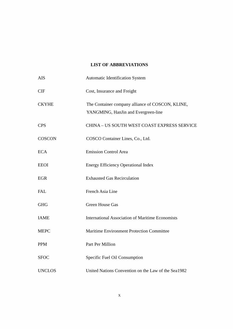
LIST OF ABBREVIATIONS

AIS Automatic Identification System

CIF Cost, Insurance and Freight

CKYHE The Container company alliance of COSCON, KLINE,

YANGMING, HanJin and Evergreen-line

CPS CHINA – US SOUTH WEST COAST EXPRESS SERVICE

COSCON COSCO Container Lines, Co., Ltd.

ECA Emission Control Area

EEOI Energy Efficiency Operational Index

EGR Exhausted Gas Recirculation

FAL French Asia Line

GHG Green House Gas

IAME International Association of Maritime Economists

MEPC Maritime Environment Protection Committee

PPM Part Per Million

SFOC Specific Fuel Oil Consumption

UNCLOS United Nations Convention on the Law of the Sea1982

11

CHAPTER 1

Introduction

1.1 Study purpose

As one of mainly purposes for engaging in the shipping industry is to pursue profit, the

better use of precious fuel should be concerned in the prevailing technology background.

The voyage profit, which means single voyage revenue minus single voyage cost and tax,

has a direct relationship to the whole interest. For making the maximum profit, one

method is focusing on the increasing revenue, while another way is by controlling the

cost. This paper centers on the second method by finding the optimization speed during

a single containership voyage as well as the whole fleet interest in a liner company.

For a given voyage under certain fixed freight rate and status, one of variables is the

speed of a ship, which can also be controlled by operation. The different speed will bring

different profit in a fixed scenario for container shipping industry. High speed may save

time by which it may bring extra revenue while it may also cause a sharp decrease of the

profit due to the excessive fuel consumption. By contrast, slow steaming may save fuel

consumption, but the customers may complain the schedule of liner particular for high

value cargoes. Further, as per the MARPOL ANNEX VI requirement, the emissions

from ships should also be controlled in various geography areas. That is why many

12

operators consider the scientific management approach regarding the fuel consumption

and its influence to marine environment.

The purpose of the study is to provide suggestions and mathematics models for the

shippers, charters or owners on selecting containership’s speed based on the analysis

case.

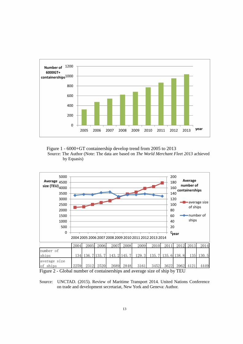
1.2 Container shipping background

The containership as an efficient transport tool has developed significantly from Feeder

to Post PANAMAX in the past thirty years (Ashar, 1999, pp.57–61.). According to the

Equasis statistics, the number of 6000+ TEU containership in 2014 has grown three

times larger than that in 2005 (See Fig -1). The total quantity of container ship

maintained in around 3500(UNCTAD, 2015, p.43) in the past ten years, while the

average ship size increased sharply from 2004 to 2014(See Fig-2). However, by

reviewing the container freight in the past five years (2000-2014), the container freight

rate is not booming as the trend of containerships’ development. By contrast, the average

of freight rate in 2014 is significantly below that of 2012 (UNCTAD, 2015a, pp.44-46).

Take the market in Trans-Pacific for example, the figure had dropped by 3.7-11.11%

(11.11% is the maximum figure appeared in the Shanghai to the US West Coast)

compared to that of 2013(Clarkson, 2014a).

13

Figure 1 - 6000+GT containership develop trend from 2005 to 2013Source: The Author (Note: The data are based on The World Merchant Fleet 2013 achieved

by Equasis)

Figure 2 - Global number of containerships and average size of ship by TEU

Source: UNCTAD. (2015). Review of Maritime Transport 2014. United Nations Conferenceon trade and development secretariat, New York and Geneva: Author.

0

200

400

600

800

1000

1200

2005 2006 2007 2008 2009 2010 2011 2012 2013

Number of6000GT+

containerships

year

020406080100120140160180200

0500

100015002000250030003500400045005000

2004 2005 2006 2007 2008 2009 2010 2011 2012 2013 2014

Averagenumber of

containerships

Averagesize (TEU)

year

average sizeof ships

number ofships

2004 2005 2006 2007 2008 2009 2010 2011 2012 2013 2014number ofships 134 136.7 135.7 143.2 145.7 129.3 135.7 135.6 138.8 135 130.5

average sizeof ships 2259 2312 2520 2689 2848 3161 3452 3622 3962 4121 4449

14

For seeking the maximum profit by decreasing the operation cost, the capacity of

containership by TEUs has increased significantly (Clarkson, 2014b), which also trigger

the market competition increasingly fierce. For example, the Maersk announced that the

Triple E series containerships with maximum capacity of 18,000 TEUs would be

serviced to the market in 2013, but no less than two years, a vessel with 19,100 TEUs

named CSCL GLOBE under the flag of China Shipping Company stepped into oceans in

early 2015. Moreover, another four ships of similar sizes are under construction (Liu,

2015). The Maersk Line did not keep silence and they planned to build six vessels of the

same level. By far, the maximum capacity of the future containership is still in doubt.

1.3 Bunkering effects

Bunkering industry has a great connection with maritime shipping, which provides the

fuel oil to the vessel (Notteboom & Vernimmen, 2009.p.325). For marine fuel sectors,

three types of fuel oil are mainly concerned to the operation of engine and ship’s

emission. MGO, shorts for marine gas oil, which is lighter fraction and better quality

compared to diesel oil, is sometime used for auxiliary engine to generate electricity

power (Lim, 1998, p.363). Marine diesel oil, also named MGO with low sulphur of less

than 0.65% is usually used for better maneuvering of main engine during inbound of

berth. Internet Fuel Oil can be divided by IFO 180 and IFO 380 for maritime transport

purpose, but the IFO180 is more expensive than IFO380 with low percentage of sulphur.

The international crude oil fluctuates in recent years due to various uncertain and

unpredictable factors. Accordingly, the marine fuel oil also changes fiercely. For

example, the price of IFO 380 in Singapore is about $330 per ton, but this figure has

reached to $700 per ton in history (Ship&Bunker, 2015). The COSCO Dalian Company

has stated that the cost of fuel accounts for 80-90% of the overall various cost according

to its own report (Wang, 2013, p.9).

15

1.4 Main Contents and Methodology

Cost structure of a single given voyage will be analyzed first aiming to clarify the fixed

cost and variable cost components. Then the relationship between speed, main engine

power and fuel consumption will be discussed in the following step.

From the perspective of main engine management, with the help of index EEOI, the

better solution for addressing the control of emission and seeking high efficiency of fuel

consumption will be found.

By analyzing the collection data, the software MS Excel will be used for comparative

analyze in factual scenario, and further simulation analysis will be carried out for

verifying the math model. The final conclusion is based on the following four aspects:

1) The actual problems of container shipping industry as well as the environment

issues;

2) The development trends of containership construction in future;

3) The necessity of specialized environment protection resolution based on the

requirement of MARPOL convention after 2015 and the operation cost related to it;

4) Discussion on the feasibility of mathematical model by using real data from

shipping companies.

16

CHAPTER 2

Literature Review

Before discussing the optimization of containership speed, the fixed speed has been

assumed in the famous RS/MS mathematics model (Rana and Vickson, 1991). But the

possible misconception is the index of speed which is treated as a fixed value in

transport. In that model, two steps were defined. Firstly, it provided the optimization

model; secondly a text of such algorithm would be conducted. Similarly, the third

research for emission in shipping sector achieved by IMO also considered the speed as a

fixed value, but it provided a comprehensive perspective for the contribution of emission

in such area (IMO, 2014a).

In this research paper, much attention should be paid to the data test which will be

explained in the real situation as the following aspects are concerned:

i. The function of fuel consumption related to the speed;

ii. The forecast scenarios under different fuel oil prices;

iii. Market and mixed chartering requirements for high speed or economic speed;

iv. Inventory cost, slot cost, etc.,

From the very beginning, the relationship between speed and fuel will be discussed.

17

2.1 The resistance and effective power functions

Fig-3 shows a simple force suffered by a floating ship. Horizontally, the resistance and

propulsion depends on the final instantaneous velocity. As early as in the year 1956, the

direct proportion between cubic of velocity and fuel consumption had been discovered

(Manning, 1956).

THRUST RESISTANCE

Figure 3 - The horizontal force of a floating shipSource: The author.

Total resistance Rt has roughly directed proportional relationship to the square of ship

velocity Vs as is shown in the following formula:

Rt = C ⋅Vs2 (1)

Here, C means coefficient.

The efficient power, which has a rough relationship with Vs, as is shown in the

following formula:

PE = RtVs = 1/2 CtρS*Vs3 (2)

(ρ : density [kg/m3] ,S : wetted surface [m2], Vs : ship speed [m/s], Ct : frictional

coefficient)

18

Res

ista

nce,

R

Pow

er,

P

Figure 4 - Resistance and effective power curves with ship speedsSource: NAKAZAWA. (2014). Impact of the maritime innovation and technology (unpublished

handout). World Maritime University.

Many researches have verified the general relationship between the fuel consumption

and speed, which can be concluded as: Fuel consumption ∝PE∝ Vs3. But this situation

does not consider whether a large containership is powered by shore electricity device

and when its speed is near zero, in most cases, it is only good for estimation of fuel

consumption (Buxton, 1985, pp.47-53). Some scholars propose a quadratic function to

estimate the consumption of fuel (Christiansen et al, 2007, pp. 189-184).

By adding another coefficient in the direct proportion function to the cubic velocity, the

function fuel consumption with velocity: Fc = K1 ×Vs + K2 means that the bigger size

vessel consume fuel faster than those smaller one (Yao, et al, 2011).

For seeking the minimum value of the triplicate integral method, a mathematical model

absent inventory cost and weather condition have been established in an average

assumption (Andersson, et al, 2015, pp. 233–240).

2.2 The operation perspective

A routing model had been assumed by the operation method used in real practice

(Fagerholt et al, 2015, pp.53-57). In this model it highlights the path thorough ECA used

for optimization speed for saving cost. This study is focusing on the math problem but

Ship speed, Vs

Rt = 1/2 C t ρSV s2

PE = RtVs = 1/2 CtρS*Vs3

19

the environmental effect is neglected. In contrast, Angelos provided the cost calculation

but without any optimization speed problem (Angelos, 2004). For better solutions of this

complex issue, some researches focus on how to determine the vessel speed dynamically

as well as refueling issues under uncertain bunker prices scenarios (Sheng et al, 2013).

In fact, the speed of ship is deeply affected by the main engine and maintenance.

2.3 Study from the perspective of marine environment protection

Engine with EGR and other equipment like hybrid turbocharger can filter the content of

NOx, and a new model of engine is set up using a power turbine can lead to 3-4% SFOC

and NOx reductions (Larsen et al, 2015, p.555).

For slow steaming approach, operation of slow steaming will bring good profit as well

as the benefit for environment (Lindstad et al, 2013, pp. 5-8). However, some people

argued that the operation of slow steaming would cause less revenue and reduce the

demand of additional ships in the market (UNCTAD, 2012). This conflicting argument

encourages a new study on how to find an optimization speed for decreasing emission as

well as operation cost (Chang & Wang, 2014, pp. 110-115).

From the policy’s perspective, as per MARPOL ANNEX Reg.14, the sulphur content

limitation of fuel oil should be no more than 0.1% inside the ECA after January 2015,

which shrinks the selection of fossil fuel.

2.4 Other elements

In practice, the weather condition seriously affects the speed in many situations, so the

whole simulate process should be based on average weather condition as many

literatures do. If a coefficient is added on such mathematics model, the coefficient

should be set up in a general situation that wave, wind, tidy and current are considered in

20

an average level.

As for maintenance, the hull and main engine condition should not be ignored. Because

the rough surface will increase the oil consumption significantly, while smooth surface

helps reduction of resistance, hence, an average hull condition is considered in the next

calculation.

Fuel price is also a potential element. If the oil price drops to a relatively low level, the

operators will pursue time rather than other elements.

Inventory cost is also another uncontrollable element for assessing the optimal speed. It

is worth to mentioning that cargo inventory costs may lead liner operators to change

their mind particularly when high valued goods are involved. For example, the price of

one unit freight of high valued goods like medical instruments ($95,000/ton, for instance)

were five time higher than that of low valued goods like furniture in 2004 (CBO, 2006).

Just assuming the delay only cost of trans- cargo in a relatively low level, for a 10,000+

containership, the money should be calculated in millions, so this result may lead to less

benefit by slow steaming(Fagerholt, 2004, 259–268.). As an important element, the

trans-cargo inventory will be discussed in the mathematics model as a special

consideration.

21

CHAPTER 3

Other Issues Regarding Operations

3.1 The various economic pressure brought by speed

Technically, the speed of containership can be categorized into normal speed, slow

steaming and extremely slow steaming (Maloni et al, 2013, p.3). Although the world’s

oil price is in a reasonable level due to the good news by the technology development

for exploration of shale oil, no one knows how it will fluctuate in the future market.

According to the Ship & Bunker data, the price of IFO180 was $319 per ton in the

February of 2015; however, this figure had jumped to over $700 per ton in history. For

better analyzing the pressure brought by the oil price, different levels of oil price are

defined. High level of price means that the fuel oil price is more than $700/ ton;

intermediate level of price means in the period between $500/ton and $700/ton;

accordingly, low level of price means less than $500/ ton. Hence, three scenarios will be

assumed as a coefficient X (X1= the real time price/ 700 in high price level, X2= the real

time price/ 600 in intermediate price level, X3= the real time price/ 500 in low price

level) in the following discussion. The first scenario will be defined as high oil price

level in which it gives a value $700X1/ton, accordingly, $500X2/ton for intermediate

price level and $300X3/ton for low price level.

For containerships of different capacity, the fuel consumption has a complex nonlinear

relationship based on statistics (See Figure 5).

22

Figure- 5: Statistics on containership fuel consumption with different speed

Source: Notteboom, T. & Carriou, P. (2009). IAME Conference, Copenhagen.

3.1.1 An example of large containership

Take the 10,000+ TEU containership as an example, the cost of fuel in different speed

can be summarized in the following table.

Table 1- Daily fuel cost in different fuel oil price by speed for 10,000+TEUcontainerships

Daily fuelcost(unit:$)

Speed

Low price level Intermediate pricelevel

High price level

Coefficient:X(X1= real timeprice / 700, X2=real time price /600, X3 = real

time price / 500)

25Kn 108000 180000 252000

22 Kn 75000 125000 175000

19 Kn 45000 75000 105000

17 Kn 30000 50000 70000

Source: The author.

Obviously, the difference on costs between the speed at 25Kn and 17Kn will reach to

$18,200X1 (X1=real time price / 700) per day. In general, the nonlinear relationship with

23

speed can be expressed by the following regression function:

y = 4666.7x3 - 24500x2 - 36167x + 308000, R² = 1 (3)

Here, y means the daily fuel cost, x means the speed of containership. The general cost

trend with ship of different speeds in different fuel oil prices can be drawn as is shown in

the following figure.

Figure 6 - Daily fuel cost in different fuel oil prices by speed for 10,000+TEUcontainerships

Source: The author.

3.1.2 The analysis for 4,000-5,000 TEU containership

Accordingly, the similar figure can be drawn the same calculation way as is mentioned

above.

$0

$50,000

$100,000

$150,000

$200,000

$250,000

$300,000

25Kn 22Kn 19Kn 17Kn

Dailyfuelcost(US

dollars)

Speed

Low pricelevel

Intermediateprice level

High pricelevel

24

Figure 7- Daily fuel cost in different oil price by speed for 40,000-50,000TEUcontainerships

Source: The author.

Any daily difference can be calculated with the following formula:

Y=1633.3x3 - 5950x2 - 29283x + 139300, (4)

Specially, x means the differential speed, while Y means the daily fuel cost which has

not been modified by the coefficient X (X1, X2, X3 for different fuel oil price scenario).

3.2 The influence to engine efficiency

3.2.1 An environment index

EEOI concerning the efficiency of ships in operations is adopted by IMO as an engine

efficiency index by which the emission of carbon dioxide can be measured per ton –

kilometer. It is calculated with the following equation:

EEOI =∑ ∗ ∗ (5)

0

20000

40000

60000

80000

100000

120000

25Kn 22Kn 19Kn 17Kn

Dailyfuelcost( US

dollars)

Speed

Low pricelevel

Intermediateprice level

High pricelevel

25

In this equation, the j is the fuel type; FCj is the mass of consumption fuel in a certain

voyage, while CFj is a convert factor from the quality of fuel to that of carbon dioxide

(IMO, 2009).

Different types of fuel will affect the value of EEOI deeply due to the various values of

CFj and carbon content (Acomi & Acomi, 2014, p.533). Basically, a smaller overall

index value means higher engine efficiency.

3.2.2 The relation between EEOI and speed

Totem Plus Company has developed software to calculate the value of EEOI. One

observation of the calculation result shows that the index decreases when the speed of a

vessel decreases simultaneously. According to the result, the difference in a same voyage

may be about 18-20% in different load condition or sailing speed (Acomi & Acomi,

2013).when the speed reduce by 10kn, the overall index will change to smaller, which

means the performance of EEOI is improved by such change (Table 2). Hence,

optimization speed can improve the EEOI by high fuel efficiency utilization ratio.

26

Table 2 - An example of EEOI CalculationSource: N.Acomia,& O.C. Acomib.(2014). The 9th International Conference on Traffic & Transportation

Studies, Shaoxing, Zhejiang Province, China.

3.3 Restriction under MARPOL convention Annex VI

For controlling the emission from ships, two general areas are divided by IMO, named

SOx-ECA and NOx and SOx-ECA area respectively (See figure 8).

27

Figure 8: Emission control area mapSource: TOCPRO(2015), MARPOL 73/78 Practical Guide

London: Author

For controlling the emission of suphur, the IMO establishes a global standard that the

content of sulphur in the fuel should be less than 3.50% from 2012, but after January1st,

2015, only the content of sulphur being less than0.1% can be used in ECAs, however,

the following steps will still continue to reduce to 0.50% from 2020 (this step may be

prolonged to 2025). Further, the marine diesel engines installed on ships should apply to

the NOX control approach which was passed through in the 66th IMO MEPC, aiming to

reduce NOX to less than 2KG/Kwh, which is nearly one eighth of the figure in 2000

(Cullinane & Bergqvist, 2014, pp.1-5). Normally, the fuel grade has directly been ralated

with the quantity of Suphur (see Tab - 3). Consequently, the oil price usually rises with

the fuel grade.

Table 3- Sulphur content in different fuel grades

Fuel Grade IFO380 & IFO180 LS180 MDO ULSFO180 LSMGO

Sulphur Content 3.50% 1. 0% 1.5% 0.10% 0.10%

Source: Ship & bunker, www.shipandbunker.com

The two mainly liner routes, namely Tans-Pacific and Fast East – Europe will be

affected dramatically by IMO new marine environment protection policy due to the

ECAs could not pass by.

3.3.1 The period from 2015 to 2020

As is mentioned above, after January 2015, when a ship enter the North American ECA,

1000 ppm sulphur content fuel oil should be used which is only one tenth of the fuel oil

that had been used before 2015. Although the limits in other pacific area can stay at

35,000 PPM level, this change will increase the cost of fuel significantly (Cullinane&

28

Bergqvist, 2014, p.3).

3.3.2 Deep influence after 2020

There will be more challenges to ship operators after the year 2020, because at that time

the suphur content may decrease to 1000PPM, which means IFO380 may not be used as

general ship fuel oil, a new standard marine fuel oil with less than 0.5% sulphur content

will replace IFO380 all over the world. Unfortunately, this will bring astonishing extra

cost for ship operators in the near future (Veenstra & Ludema, 2006, pp.159-171). But

for marine environment, it is completely good news.

29

CHAPTER 4

The Mathematic Model for Optimal Speed

4.1 The major premise of this problem

The general cost of a container fleet includes the operation cost, capital cost, inventory

cost, fuel cost and port charges (Fagerholt, 2004, p.36). The inventory cost, capital cost

and fuel cost has a close relationship to the speed, this chapter is aiming to decrease fuel

cost by the adequate operation approach for ship operators except the inventory cost

which will be discussed in the following chapter. The average weather condition is the

first premise for this problem, and fuel price is also to be defined according to the

prevailing price in the market. Assuming the operators will abide by the convention for

the restriction in the ECA, the main mathematics parameters can be expressed (See

Table 4):

Table 4-The parameters used in the mathematic model

parameters Descriptions

pE MGO inside of ECA

fE Fuel consumption per day when ship proceeding in ECA with alternative speed v

30

tE Time of ship navigate in ECA with alternative speed v by day

pG Fuel oil price in Non-ECA

fG Fuel consumption for global navigation in Non-ECA

tG Time of ship navigate out ECA

Source: The author

The main purpose is to seek the minimum value in the following formula:

Min {[ +(1 + ) ]} (6)

4.1.1 The bunker consumption function

As is mentioned above, the bunker consumption has direct proportional relationship with

the cubic velocity, but this function had been rectified by two coefficients based on the

data acquired from the shipping liner company (Yao, et al, 2011).

= < 8,000 , = +≥ 8,000 , = 0.087 (7)

This function will be used by inputting the different coefficients in various velocity (See

Tab -5).

Table 5- K1,K2 coefficients are listed by various containership capacity

31

Source: Zhishuang Yao et al (2011). A study on bunker fuel management for the shipping linerservices. Computers & Operations Research.

However, the limitation of this statistic does not provide more details if the size of

containership is over 8,110 TEU. For calculation of the ship over 8,000TEU, here a new

specified coefficient K3 is given (See Table - 6).

Table 6 -The coefficient K3

Size (TEU) Value of K3

8,000-9,000 3.21

9,000-10,000 3.24

10,000+ 3.30

Source: The Author.1

4.1.2 The value of total trip time

The container liner company always put several sister-ships on the same line in order to

fulfill their schedule, so the service frequency in mostly situation is fixed (Ting &Tzeng,

2003, p.381). The routing is not like tramp shipping, actually it is a loop routing or cycle.

Once a schedule has been published to the public, the ship operator will push the service

1 Note: Please refer to Appendix I for the details of calculation.

Size(TEU) K1 K2

1000- 0.004476 6.171000-2000 0.004595 16.422001-3000 0.004501 29.283001-4000 0.006754 37.324001-5000 0.006732 55.845001-6000 0.007297 71.46001-8000 0.006705 87.71

32

at least for one week unless a new turn of market assessment begin.

So the total trip time: T = ∑ + ∗ (8)

Here, ∑ means the total port time, Vmax is the maximum sea speed, Vs is a discrete

value which is subjected to VS ∈ Vmax.

4.2 Mathematics model

The model is based on the assumption that the very operation day contributes to the

same amount of cost which includes the capital cost of a company in one service cycle.

4.2.1 The model in non-ECA areas

Table 7 - The notations of the mathematics model

notations Descriptions

pE MGO inside of ECA

fE Fuel consumption per day when ship proceeding in ECA with alternative speed v

tE Time of ship navigate in ECA with alternative speed v by day

DE Distance navigated in the ECA

DC Distance for preparing berth in Non - ECA

pG Fuel oil price in Non-ECA

pm MDO price, MDO may be used before berth for better maneuver

fG Fuel consumption for global navigation in Non-ECA

tG Time of ship navigate out ECA

DG Distance navigated out of ECA

T Overall trip time by days

Overall time in port by days

Te Time for navigating in the ECA by days

33

Tg Time for navigating outside of ECA by days

Vs The discrete speed of vessels

Ve The average ship’s speed in the ECA

Vg The average ship’s speed outside of ECA, a normal speed in the global waters

Vmax The maximum speed of a certain containership

fc(V) Fuel cost function with the variable value speed

Source: The Author

Maximize: pmax(v) =

R − C − ∗ ∗ ∗∑ ∗R − C − ∗ . ∗ ∗∑ ∗(9)

Subject to: , , < Vmax ;

∗ + ∗ = ;+ = ;+ = ;=

∗ + ∗ ∗∗ 0.087 ∗ ∗Here pmax means the maximum profit function with the variable value , while R means

the revenue of a voyage or a cycle; C means the average fixed cost including the

(If container capacity is less than8,000TEU)

(If container capacity is more than8,000TEU)

(If containers capacity is more than8,000TEU)

(If container capacity is less than8,000TEU)

34

capital cost, manning cost and maintenance cost, port changes, tug fee, etc., means

the correction of MGO cost for better maneuvering in non – ECA when preparing for the

berth operation.

4.2.1 The model for a ship passing through ECA

Similarly, for seeking the maximum profit, the equation can be expressed as:

pmax(v) =

R − C − ∗ ∗ ∗ ∗ ∗ ∗∑ ∗ ∗R − C − ∗ . ∗ ∗ ∗ . ∗ ∗∑ ∗ ∗(10)

Particularly, the general fuel cost function combined with ECA route is:

fc ( , ) =

∗ ∗ ∗ ∗ ∗ ∗∑ ∗ ∗∗ . ∗ ∗ ∗ . ∗ ∗∑ ∗ ∗(11)

4.3 Value of simulation

4.3.1 Fuel price

The fuel price always changes in various supply ports. Considering the mainly routing

and the probability of ECA passing through in the word, the average price in the

(If container capacity is lessthan 8,000TEU)

(If containers capacity ismore than 8,000TEU)

(If container capacity is less than8,000TEU)

(If container capacity is more than8,000TEU)

35

Rotterdam and Houston are used for analysis. The fuel price may fluctuate frequently in

the market, and the relationship between ship routing and speed is similar in the model.

According the Ship & Bunker price in April 2015, the average price of IFO180 in

Rotterdam and Houston is $405/ton and the average MGO in the same place is $ 590/

ton for the analysis of standard scenario. But after 2020, the more strict regulation

requires high quality of marine fuel oil which generates less sulphur dioxide. Normally,

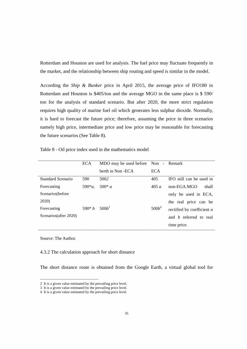
it is hard to forecast the future price; therefore, assuming the price in three scenarios

namely high price, intermediate price and low price may be reasonable for forecasting

the future scenarios (See Table 8).

Table 8 - Oil price index used in the mathematics model

ECA MDO may be used before

berth in Non -ECA

Non -

ECA

Remark

Standard Scenario 590 5002 405 IFO still can be used in

non-EGA.MGO shall

only be used in ECA,

the real price can be

rectified by coefficient a

and b referred to real

time price.

Forecasting

Scenarios(before

2020)

590*a, 500* a 405 a

Forecasting

Scenarios(after 2020)

590* b 500b3 500b4

Source: The Author.

4.3.2 The calculation approach for short distance

The short distance route is obtained from the Google Earth, a virtual global tool for

2 It is a given value estimated by the prevailing price level.3 It is a given value estimated by the prevailing price level.4 It is a given value estimated by the prevailing price level.

36

providing the geography information. The cases are retrieved from the real service on

the web site of COSON which illustrates the main business conducted in the global

scope.

4.4 Cases text

The following two examples contain two different mathematic models discussed above.

4.4.1 Tans - Pacific service: CPS Route

The CPS service is one of most important Tans – Pacific route which is linked with the

logistics between Eastern China and the Southwest Coast of U.S (COSON, 2015). The

loop begins from the port Qingdao, Shanghai, and Ningbo to Los Angles in California

State, and then returns to port Qingdao, China through the transport of Oakland (see

Figure 9).

37

Figure 9 – Ports of call under CPS RouteSource: COSOCN. (2015). http://www.coscon.com/schedule/schedulecn.jsp

In this loop, the main ECAs are located in the US jurisdiction waters (See Figure 9)

where are inescapable areas for ships to pass through. The shortest path for passing

through this area is 230 nautical miles, but the reasonable deviation in practice should be

considered. Therefore, the data 250 nautical miles is adopted in the following analysis.

38

Figure 9 - Geographical Distribution of ECA in CPS routeSource: IMO. (2010). MEPC.1/Circular.723, London, UK.

The loop of CPS service is from the Qingdao, China to Los Angles, California, in the

middle way of which Shanghai and Ningbo will be berthed as a transshipment port. The

legs in different ports categorized by ECA and Non – ECA scenarios are listed (See

Table 9). Additionally, the containership always change MDO when she approaches to

the berth, so 10 nautical miles is assumed for her change from IFO to MDO before she

arrives at to the berth. This distance will be treated the same way as she proceeds in the

ECA because the same fuel oil (MGO) is used for better maneuver.

Table 9 - Distance of route legs

Legs Distance (unit: nautical miles)ECA Distance for use

MGO whenprepare for berth

Non - ECA Total

Qingdao – Shanghai 0 20 379 399Shanghai – Ningbo 0 20 150 170

39

Ningbo – LosAngles

250 10 5,936 6,166 *

Los Angles –Oakland

369 0 0 369

Oakland - QingDao 300 10 5,098 5,408

The cycle 12,512Source: The author, note: “*” means the data is retrieved from http://www.sea-distances.org/

Due to the fact that eight of ten containerships engaging on the CPS service are over

8000TEU capacity (See Table 10), the coefficient K3 shall be used. With regarding to the

other two vessels, the coefficient K1, K2 can be referred to calculation result at the

beginning of this Chapter where K1 equals 0.006705 and K2 equals 87.71.

Table 10 - CPS service Schedule

Vessel Voyage Port ATA/ETA ATD/ETD Distance cycle time(days)

Size(TEU)

EVERURSULA

0635E Ningbo/Los

Angeles

2015-2-1621:20

2015-3-264:15

6166 37.288 5652

EVERLOGIC

0637E Qingdao/Los

Angeles

2015-3-52:40

2015-4-24:07

6735 28.060 8452

EVERLUCID

0638E Qingdao/Oakland

2015-3-1116:40

2015-4-103:43

7104 29.460 8508

EVERLEARNED

0642E Qingdao/Oakland

2015-4-820:30

2015-5-14:00

7104 22.312 9200

EVERLIBERAL

0643E Qingdao/Oakland

2015-4-1515:30

2015-5-108:00

7104 24.687 8452

EVERCONQUEST

No data 8073

ITALCONTESSA

8073

EVERLUCKY

8452

EVERLASTING

8452

40

EVERUNITY

5652

Source: www. COSCON.com & www. evergreen-marine.com

a) Standard Scenario – fuel oil price in the current level

The vessel EVER URSULA and vessel EVER LOGIC will be taken as an example since

this route involves two types of containerships.

i. M/V EVER URSULA

Table 11- The service data of M/V EVER URSULA

Port ATA ATD porttime(days)

at sea(days)

Distances(nmiles)ECA Distance for

use MDO whenprepare for

berth

Non-

ECA

Ningbo 2015-2-1621:20

2015-2-1714:00

0.694 0 10 0

Shanghai 2015-2-223:00

2015-2-2214:00

0.458 4.542 0 20 140

Qingdao 2015-2-247:40

2015-2-2414:40

0.292 1.736 0 20 379

LosAngeles

2015-3-236:00

2015-3-264:15

2.927 26.639 250 10 5706

Port time: 4.372 days,At sea time: 32.917days.

Average speed:9.24 kn, ve=9.32 kn, vg= 9.21 kn

Source: The Author (Note: Data of ATA&ATD are based on the Evergreen-marine International

Service).

Evergreen Company set up the line schedule in CPS service based on 21.667 days from

Qingdao to Los Angles. Since the vessel is less than 6000TEU, the following equation

shall be applied (see calculation details in the Appendix II):

41

, = ∗ ∗ ∗ ∗ ∗ ∗∑ ∗ ∗ ∗ ( = 0.006705, = 87.71 )

=∗ . . ∗ ∗ ∗ . . ∗ ∗ ∗ . . ∗ ∗. ∗ ∗ ∗

Subject to: , < ;∑ + ∗ + ∗ + ∗ =T (12)( ) Function curve of M/V EVER URSULA can be drawn combined with the Vg

Function curve based on the calculation result of Appendix II (Figure 10).

Figure 10 - The ( ) function curve of M/V EVER URSULA

Source: The Author.

The lowest point of ( ) function curve in standard scenario implies minimum fuel

cost where the optimize speed of the M/V EVER URSULA in ECA is 16.75 kn and the

speed out of ECA is 15.73 kn. Both of them are relatively higher than the real speed.

15.4

15.5

15.6

15.7

15.8

15.9

16

16.1

16.2

16.3

16.4

37500

37600

37700

37800

37900

38000

38100

38200

38300

8 9 10 11 12 13 14 15 16 17 18 19 20 21 22 23 24 25 26 27

Vg(kn)Daily fuel oilcost($)

Ve

fc instarndardscenario

Vg

42

That means if the company does not improve the prevailing speed it may not catch up

with the schedule as it promises on the Internet.

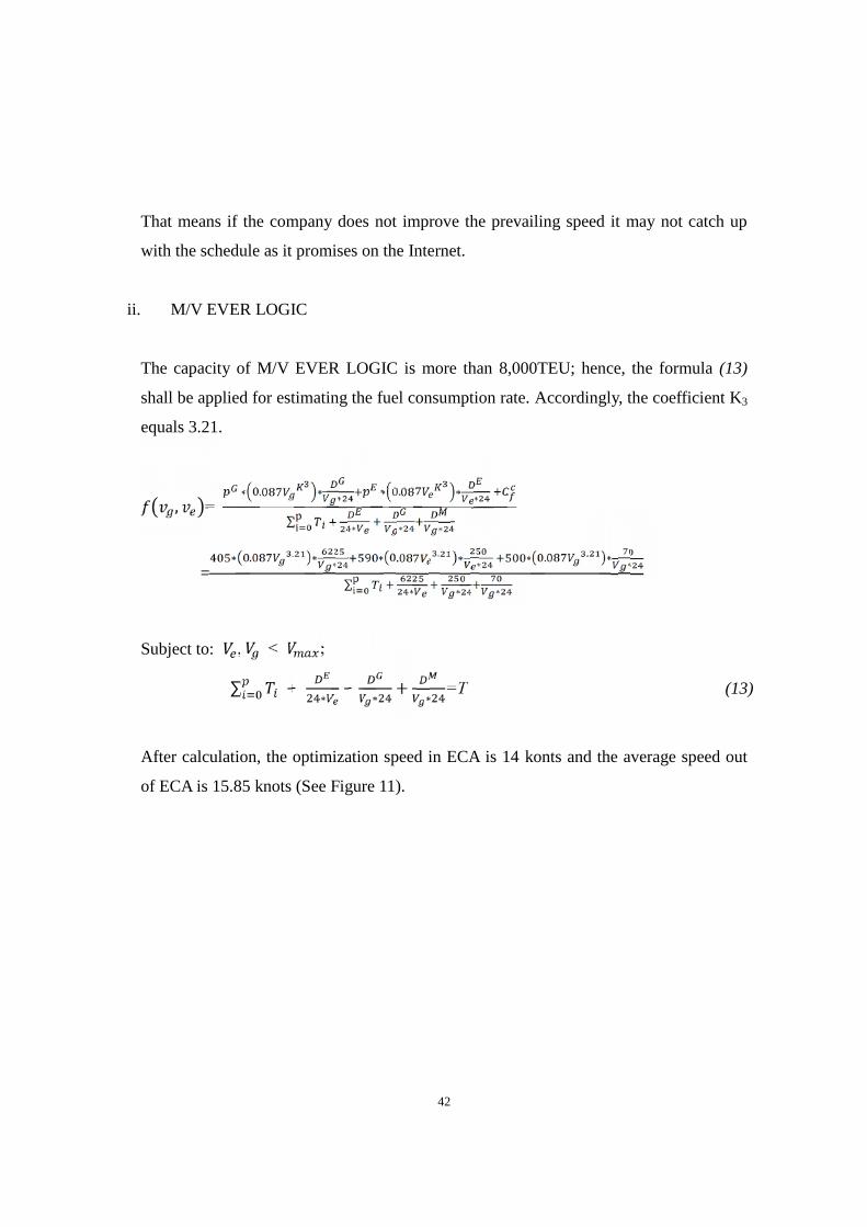
ii. M/V EVER LOGIC

The capacity of M/V EVER LOGIC is more than 8,000TEU; hence, the formula (13)

shall be applied for estimating the fuel consumption rate. Accordingly, the coefficient K3

equals 3.21.

, =∗ . ∗ ∗ ∗ . ∗ ∗∑ ∗ ∗ ∗

=∗ . . ∗ ∗ ∗ . . ∗ ∗ ∗ . . ∗ ∗∑ ∗ ∗ ∗

Subject to: , < ;∑ + ∗ + ∗ + ∗ =T (13)

After calculation, the optimization speed in ECA is 14 konts and the average speed out

of ECA is 15.85 knots (See Figure 11).

43

Figure 11 - The calculation result of M/V EVER LOGIC

Source: The Author.

b) The virtual scenario in different oil prices for the CPS service

In addition to the standard scenario with the estimated price applied in the math model,

three possible virtual scenarios are analyzed. As is expected, the overall cost will

increase accordingly (See Figure 12 and Figure 13). The difference between the two

trends is that, for M/V EVER URSULA, the effect brought by optimal speed in ECA is

becoming less and less with the speed increase because the weight of ECA legs are

relative smaller particular when the oil price rises up. The operator will have more space

for selecting adequate speed out of ECAs.

15.4

15.5

15.6

15.7

15.8

15.9

16

16.1

16.2

16.3

16.4

198000

200000

202000

204000

206000

208000

210000

212000

214000

216000

218000

8 9 10 11 12 13 14 15 16 17 18 19 20 21 22 23 24 25 26

Vg(kn)daily fuel oilcost($)

Ve

fcchangesby Ve

vg

44

Figure 12- The ( ) function curve changes by different virtual scenario of M/V

EVER URSULA

Source: The Author.

By contrast, for large ships more than 8,000 TEUs, if the oil price rises up, the influence

caused by ECAs will still be relatively strong with optimal point moving forward as is

shown in the graph. Ship operators may pay more attention in this scenario and it may be

operated through a whole year.

37000

39000

41000

43000

45000

47000

49000

51000

8 9 10 11 12 13 14 15 16 17 18 19 20 21 22 23 24 25 26 27

daily fuel cost($)

Ve

fc in standard scenario

when oil price rise 10%before 2020

fc in forecasting scenarionafter 2020 whena1=1,b1=1

fc in forecasting scenarionafter 202 when oil averageprice rise 10%

45

Figure 13- The ( ) function curve changes by different virtual scenario of M/V

EVER LOGIC

Source: The Author.

c) Summary of CPS service

Basically, the loop of this route is 57 days. The number of ships deployed in this route

should meet the current requirement based on the schedule published to the customers

(Karlaftis et al, 2009.p.210). According to the company public plan, the ports in this

route will be called at least once per week, 8 vessels should be deployed on this route,

but in factual practice, 10 vessels are servicing on this line (See Table 12).

Table 12 - Calculation result of the CPS Service

190000

200000

210000

220000

230000

240000

250000

260000

270000

280000

290000

8 9 10 11 12 13 14 15 16 17 18 19 20 21 22 23 24 25 26 27

Daily fuel oilcost($)

Ve(kn)

fc changes by Ve

when oil price rise10% before 2020

fc in forecastingscenarion after 2020when a1=1,b1=1

fc in forecastingscenarion after 202when oil averageprice rise 10%

46

Deployment Speed

in

ECA

Speed

out of

ECA

Cost($) Difference for

single vessel

($/day)

Difference

for

fleet($/day)

Optimal

Resolution 1

Two 6000TEU

vessels

16.75 15.73 37581*

2

increase

$4127/day

Save

$ 416882

Six

8000+TEUvessels

14 15.85 200288*6

save$12/day

OptimalResolution 2

Eight 8000+ TEUvessels

14 15.85 200288*8

save$12/day Increase

$87686/day

Current Two 6000TEUvessels

9.24 9.21 33454*2

- 1669228

Eight 8000+ TEUvessels

14.26 13.21 200290*8

-

Source: The Author.

For determining the optimal speed, the introduction of ECAs is one of the elements due

to the extra fuel consumption cost by compliance with the environment policy

(Doudnikoff &Lacoste, 2014, pp. 19-29). The optimal number of vessels servicing on

the same route is another important concern. In the given CPS real practice, there are

two optimal solutions to eight vessels engaging in service.

i. Assuming the two containerships less than 8,000GT and six 8,000+GT

containership service in this route as the original deployment

This scenario is based on the fact that overall transportation demands do not change

obviously, so the revenue keeps in a relative steady level. The purpose of this method is

to control the overall cost and be competitive ability in the market simultaneously. By

calculation, the daily cost will be saved $416,882 per day for the whole fleet.

ii. Assuming eight 8,000+ TEU containerships engaging in service

47

This solution is from the perspective of revenue increase by using mega vessels with

8,000+ capacity TEUs. Although the overall cost will increase by substituting the

smaller vessel, the transport efficiency and revenue will increase as more cargo will be

loaded on vessels. Hence, this solution may be adopted when the freight rises up or the

anticipated profit becomes better in operation.

4.4.2 Asia – Europe service: FAL_1 Route

Asia – Europe is very significant particularly when China proposes “the Silk Road

Economic Belt” strategy (Xi, 2013, para.12). As a link between the Far East and Europe,

many famous P3 or CKYHE member companies like MARSK, CMA CGM, and

COSCON are paying more attention to Asia – Europe business. Beside the cooperation,

they compete for acquiring the maximum profit in the big cake.

There are 13 ports involving shipment service on the FAN_1 route (See Figure14).

48

Figure 14 -The FAL_1 Service diagram

Source: COSCON. (2015b). FAL_1 Service (http://www.coscon.com/)

Shanghai: Author.

The five European ports, namely Southampton, Hamburg, Rotterdam, and Le harve

where are all located in the North Sea ECAs restrict the emission of NOX and SOX from

ships (See Table 13). Consequently, the quality of fuel oils loaded should meet with

much stricter requirement under MARPOL ANNEX VI.

Table 13 - The distances by legs on FAL_1 Route

Legs Distance (unit: nautical miles)ECA Distance for use

MGO when preparefor berth

Non - ECA Total

Ningbo – Shanghai 0 20 150 170Shanghai – Xiamen 0 20 565 585

Xiamen – Hong Kong 0 20 267 287Hong Kong – Chiwan 0 35 0 35

Chiwan – Yantian 0 20 110 90Yantian – Kelang 0 20 1,650 1,670

Kelang – Southampton(through Suez canal)

330 20 7,521 7,871*

Southampton- Hamburg 505 - 0 505*Hamburg – Rotterdam 305 - 0 305*Rotterdam –Zeebrugge 87 - 0 87*Zeebrugge – Le harve 181 - 0 181*

Le harve –Ningbo (throughSuez canal)

210 - 10,090 10,300

The cycle 22,086Source: The Author, “*” means the data is based on http://www.sea-distances.org/

a) Standard Scenario – fuel oil price in the current level

Nine over 80,000TEU CMA CGM containerships are deployed on the FAL_1 line, five

49

of which are sister ships with the capacity of 13,830 TEU (see Table 14).

Table 14 -The statistic of containerships of CMA CGM servicing on the FAL line

Vessel Voyage Port ETA ATD cycle time

(days)

Size

(TEU)

CMA CGM

AMERIGO

VESPUCCI

FLB24W/

FLB45E

Ningbo 2015-4-23

21:00

2015-1-29

23:59

83.9 13,830

CMA CGM

NEVADA

FLB26W/

FLB47E

Ningbo 2015-4-29

2:00

2015-2-5

14:00

82.5 12,552

CMA CGM

JULES VERNE

FLB28W/

FLB49E

Ningbo 2015-5-6

0:00

2015-2-16

12:00

78.5 16,022

CMA CGM

GEMINI

FLB30W/

FLB51E

Ningbo 2015-5-13

12:00

2015-2-19

22:00

82.6 11,388

CMA CGM

CORTE REAL

FLB34W/

FLB53E

Ningbo 2015-5-20

2:00

2015-3-5

6:00

75.8 13,830

CMA CGM

CHRISTOPHE

COLOMB

FLB36W/

FLB55E

Ningbo 2015-5-21

2:00

2015-3-12

1:00

70 13,830

CMA CGM

LAPEROUSE

FLB38W/

FLB57E

Ningbo 2015-6-10

0:00

2015-3-20

9:00

81.6 13,830

CMA CGM

MARCO POLO

FLB40W/

FLB59E

Ningbo 2015-6-17

2:00

2015-3-26

14:00

82.5 16,022

CMA CGM

MAGELLAN

FLB42W/

FLB63E

Ningbo 2015-7-8

0:00

2015-4-24

14:20

74.4 13,830

Source: COSCON Office & CMA CGM. (2015). COSCON Office Materials. Shanghai,China.

(note:the data of ship size areretrieved from: http://www.cma-cgm.com, others are

retrieved from COSCON Office located in Shanghai).

50

Obviously, all the vessels deployed on this route are over 8,000 TEUs, and the

coefficient k3 should be used for estimating the fuel consumption in standard scenario.

Since five of nine ships are sister-ships with same the capacity(13,800 TEU), the 365.5

meters length of all with 51.20 meter beam vessel named CMA CGM AMERIGO

VESPUCCI whose summer dead weight can reach to 156,887 tons will be taken as an

example in the following analysis (CMA CGM, 2015) (See Table 15).

Table 15 -The actual service voyage FLB24W/ FLB45E of M/V CMA CGM AMERIGO

VESPUCCI deployed on the Asia – Europe line

Port ATA ATD porttime

(days)

at sea(days)

distances(nmiles) speed

ECA Distancefor useMGOwhen

preparefor berth

Non -ECA

Ningbo 2015-1-2

8 11:00

2015-1-2

9 23:59

1.541 0 10 0 14.14

Shanghai 2015-1-3

0 12:00

2015-1-3

1 10:00

0.917 0.501 0 20 140 14.15

Xiamen 2015-2-1

15:30

2015-2-2

7:50

0.681 1.229 0 20 565 19.83

Hong Kong 2015-2-3

12:05

2015-2-4

5:15

0.715 1.177 0 20 267 10.16

Chiwan 2015-2-4

7:30

2015-2-4

22:30

0.625 0.094 0 35 0 15.56

Yantian 2015-2-5

6:20

2015-2-5

22:35

0.677 0.326 0 20 90 14.04

Port

kelang

2015-2-9

13:55

2015-2-1

0 11:10

0.885 3.639 0 20 1650 19.12

Southampt

on

2015-3-2

8:29

2015-3-3

11:50

1.140 19.888 330 20 7521 16.49

Hamburg 2015-3-5

7:38

2015-3-6

21:49

1.591 1.825 505 0 0 11.53

51

Source: The Author.

Similarly, because all giant ships are over 8,000TEUs, the fuel consumption function

coefficient should be referred to second part of the formula 11:

, = ∗ 0.087 ∗ ∗ 24 + ∗ 0.087 ∗ ∗ 24 +∑ + 24 ∗ + ∗ 24Subject to: , , < Vmax;+ = ;

= ∗ 0.087 ∗ ∗ . (14)

Even some engines can be operated appropriately at the 10–25% load region (Guan et al,

2014, p.382), typically, for a containership, the persistent sea speed should not be less

than 9 knots for better protection of main engine particularly for very large ship over

10,000 TEU. Therefore the range of speed value is calculated from the 9 knots to its

maximum design speed and the detailed calculation result is listed on the Appendix II.

The low point of the two curves ( ) with variable distributed in the transversal

direction shows the minimum value of cost in terms of speed in ECA on average (See

Figure 15).

Rotterdam 2015-3-7

22:02

2015-3-9

7:27

1.392 1.009 305 0 0 12.59

Zeebrugge 2015-3-9

14:00

2015-3-1

0 4:35

0.608 0.273 87 0 0 13.28

Le Havre 2015-3-1

0 21:48

2015-3-1

1 21:11

0.974 0.717 181 0 0 10.51

Ningbo 2015-4-2

3 21:00

42.992 210 0 10300 10.19

Overall port time: 11.746 days, overall sea time: 73.671days.average speed:12.62 kn;

average speed in ECA = 12.22kn;average speed out of ECA =12.55kn

52

Figure 15 -The ( ) function curve in standard scenario and Vg curve changes by Ve

for FAL_1 Service

Source: The Author.

The optimization of speed in the standard scenario happened where the equals 11.5

knot and equals 12.7 knots considering opportunity cost by the correction of

maneuver MDO consumption and the port time.

b) The virtual scenario in different oil prices for the FAL_1

Given the coefficient a1 =1 in different price scenario, the ( )curve has similar

property that in the vicinity if 11.5 knots the overall fuel cost reaches to the lowest point

(See Figure 16). The reason caused by this phenomenon is attributed by the different

12.0

12.2

12.4

12.6

12.8

13.0

13.2

13.4

0

20000

40000

60000

80000

100000

120000

140000

160000

180000

200000

7 8 9 10 11 12 13 14 15 16 17 18 19 20 21 22 23 24 25

speed of Vg

fueloil

cost(US

Dollars)

the speed of Ve

fc instandardscenario

vg

53

weight legs in the given route that the Non – ECA leg takes 92.75% (20,698 nmiles in

Non – ECA legs).

Figure 16 - ( ) function curves in different oil price scenario for FAL_1 Service.

Source: The Author.

c) The assessment of deployment in the FAL_1 service

The average cycle time of FAL_1 service is 79 days, according to the schedule of the

CMA CGM. The frequency of a single port called by the fleet is one week one time

which is under the considering of shipper’s demand in the market. A certain threshold of

a fixed liner service should not exceed a given frequency with certain numbers of ships

130000

140000

150000

160000

170000

180000

190000

200000

210000

220000

9 10 11 12 13 14 15 16 17 18 19 20 21 22 23 24 25

unit: $/day

Ve

fc in standardscenario

when oil pricerise 10% before2020

fc in forecastingscenarion after2020 whena1=1,b1=1

fc in forecastingscenarion after202 when oilaverage pricerise 10%

54

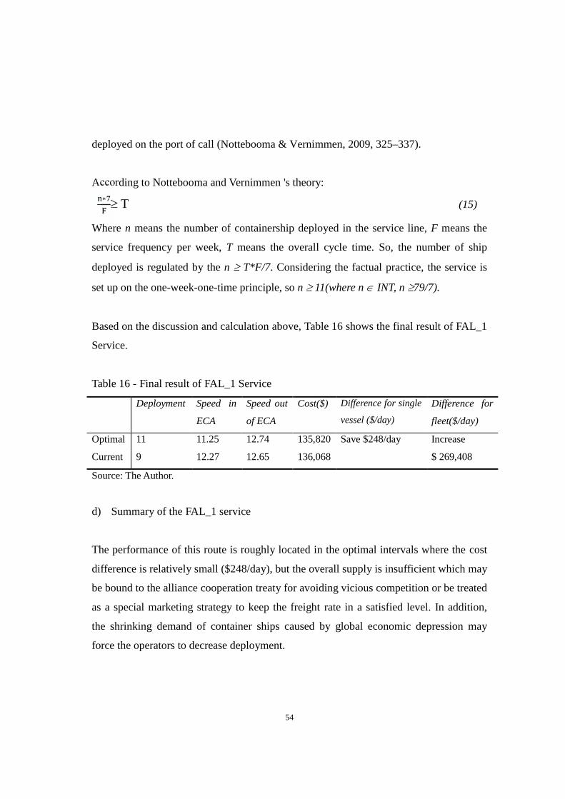
deployed on the port of call (Nottebooma & Vernimmen, 2009, 325–337).

According to Nottebooma and Vernimmen 's theory:∗ ≥ T (15)

Where n means the number of containership deployed in the service line, F means the

service frequency per week, T means the overall cycle time. So, the number of ship

deployed is regulated by the n T*F/7. Considering the factual practice, the service is

set up on the one-week-one-time principle, so n 11(where n INT, n 79/7).

Based on the discussion and calculation above, Table 16 shows the final result of FAL_1

Service.

Table 16 - Final result of FAL_1 Service

Deployment Speed in

ECA

Speed out

of ECA

Cost($) Difference for single

vessel ($/day)

Difference for

fleet($/day)

Optimal 11 11.25 12.74 135,820 Save $248/day Increase

$ 269,408Current 9 12.27 12.65 136,068

Source: The Author.

d) Summary of the FAL_1 service

The performance of this route is roughly located in the optimal intervals where the cost

difference is relatively small ($248/day), but the overall supply is insufficient which may

be bound to the alliance cooperation treaty for avoiding vicious competition or be treated

as a special marketing strategy to keep the freight rate in a satisfied level. In addition,

the shrinking demand of container ships caused by global economic depression may

force the operators to decrease deployment.

55

CHAPTER 5

Perspective from Different Points of View

5.1 The pressure of marine environmental protection

The third GHG research shows that the shipping sector accounts for about 3.1% of the

annual global emission from 2007 to 2012 on average (IMO, 2014, p.16). In the

shipping sector, container shipping has been the biggest sector of emission and may

continue its growth in the next few decades (IMO, 2009b). 16 different scenarios are

developed in 2050 by IMO, showing that the emission will increase from 50% to 250%

(IMO, 2014, p.164); the environment pushes the shipping innovation by decreasing the

fossil fuel or by conducting more strict emission regulations.

The calculation quantity on the carbon dioxide is based on the equation that every ton of

heavy fuel oil will generate 3,021 grams of CO2 and every ton of marine gas oil will

generate 3,082 grams CO2 (Psaraftis & Kontovas ,2013). Although the uncertain bunker

prices causes a scenario tree structure for calculation (Sheng et al, 2015, p.76), assuming

that 20 tons of MDO are consumed for electricity generators per day in 8,000+ TEUs

containerships, it can get the mass of emission function with speed: (V) =

3.021*0.087* V +3.01*20, which is very similar to the fuel consumption by moving

56

the whole graph towards the vertical direction in coordinate system. It also happens in

the vessel less than 8,000 TEUs, as the fuel consumption have certain relationships with

the ship’s speed. Hence, the reduction of carbon dioxide also has similar a non-leaner

relationship as is mentioned above.

The potential emission reduction for an attainable ship speed in a specific route can be

estimated. The optimization could be based on the requirement of environment rules and

operation. It will not only bring the economic profit but also be beneficial to the air

condition. From that point of view, the overall reduction of emission will also benefit

from the optimal speed.

5.2 Performance of containerships by assessing the index

The speed of containership also affects the general transport efficiency which is

expressed by the index where P means the average engine power of the

containership fleet and V means the averages speed in service. Assuming the minimum

resistance effects on ship, the index has a nonlinear relationship with (NAKAZAWA,

2014, p.74). From a global perspective, the trend of average [5] value is becoming

smaller, which implies the transport efficiency has become well. In another word, the

fierce competition in the container shipping sector also becomes obvious (See Figure

17).

[5] The calculation result and parameters are listed on the Appendix VI.

57

Figure 17 - Average of value P/WV for container ships in global scopeSource: The Author.

For a given route, like the CPS and FAL_1 service mentioned above, the optimal speed

may apparently decrease the transport efficiency, but considering the whole fleet,

optimal speed effected the actual performance of power and load ability through which

the transport efficiency increase accordingly. Relative emissions of GHG from

containerships (kg/t km) have a deep connection with capacity utilization which is very

sensitive to transport efficiency (Prpic-Orsic´& Faltinsen, 2012, p.9). Indeed, the value

of can be referred to as a kind of marine environmental protection index to some

extent.

5.2 Time and circumstances for considering the inventory cost

The inventory cost is usually caused by human operation, compared to the limited

actions conducted on capital cost, which can be decreasing as reasonable level as

possible via adequate operations.

0.0250.0260.0270.0280.029

0.030.0310.0320.0330.0340.0350.0360.0370.0380.039

0.040.0410.0420.0430.0440.0450.0460.0470.0480.049

0.050.0510.0520.0530.0540.055

0-999 1000-1999 2000-2999 3000-4999 5000-7999 8000-11999 12000-14500

P/

WV

2007

2008

2009

2010

2011

Capacity ofcontainerships

58

5.2.1 The inventory estimated by the average level

In 2014, the overall value of global container trade with a total number of 170 million

TEUs reaches to 56,000 billion US Dollars (UNCTAD, 2015, p.69), which means one

single container cargo is worth $32,941 on average (56,000 billion/170million TEUs).

The international return rate is much higher than loan rate, for inventory cost, 20% is

usually used for calculation (Bergh, 2010, pp.10-13).

Take 13,800 TEUs vessel CMA CGM AMERIGO VESPUCCI in FAL_1 line for

example, assuming that 20% cost is caused by the trans-cargo inventory and the load

rate is 80%, the number will be $249,088/day (20%*13,800 TEUs*$32,941/365days for

a year). Even a charterer in a CIF trade mode would select a faster vessel for quicker

delivery of cargoes.

5.2.2 Time to consider the trans- cargo inventory from a shipper perspective

The time for adjusting the speed of containership is depended on the freight rate in the

international trade. Extra freight may be got from high value cargo then extra fuel cost

can be considered in a given voyage. Still take the vessel CMA CGM AMERIGO

VESPUCCI in FAL_1 line for example, Figure 18 shows the optimal speed in normal

situation. A reference line drawn in the longitudinal direction mean the extra cost can be

added for quicker a delivery of cargoes and the difference between optimal point cost

and vertical value crossed with the reference line is the extra cost for getting more

revenue by minimizing the cargo owners’ inventory cost.

59

Figure 18 - The selected speed after considering the inventory costSource: The Author

By drawing a reference line, a new Ve, Vg can be obtained from the table. Sometimes it

may get two groups of Ve and Vg, and the value adopted is determined by the geography

position of cargo for delivery and ship’s position.

5.3 Questionnaire accomplished by cargo agencies

For better assessment on the service level of company and cargo delivery, a

questionnaire is designed by the author to find the critical issues involving the speed

from the cargo agencies perspective.

5.3.1 Questionnaire table

Q1. What do you think of the general performance of global liner service?

12.0000

12.2000

12.4000

12.6000

12.8000

13.0000

13.2000

13.4000

0

20000

40000

60000

80000

100000

120000

140000

160000

180000

200000

7 8 9 10 11 12 13 14 15 16 17 18 19 20 21 22 23 24 25

speed of Vg

fueloil

costby US

dollars

the speed of Ve

fc instandardscenario

vg

Ve'

REFERENCE LINE

60

Good □ Acceptable □ Poor□

Q2. What do you think of the ship speed in Trans – Pacific service?

Fast □ Normal □ Slow□ Extremely Slow□

Q3. What is the reasonable freight for Trans – Pacific service ($/FEU) by your knowledge?

900-1200□ 1200-1500□ 1500-1800□ 1800-2200□ Others□

Q4. What do you think of the ship speed of the Asia – Europe Service?

Fast □ Normal □ Slow□ Extremely Slow□

Q5.What is the reasonable freight for Asia –Europe service ($/TEU) by your knowledge?

900-1200□ 1200-1500□ 1500-1800□ 1800-2200□ Others□

Q6. Which are the first three options should be considered when your select liner service?

(Multiple – choice question)

Safety □ Reputation □ Cargo delivery □ Service speed □ Freight □

Port to call □

Q7. What is the most important factors for selecting business partner?

A company with fixed schedule □

A company which provides fast transport service but the schedule is always changed □

Table 17- Questionnaire for the liner service

Source: The Author.

5.3.2 Data analysis

58 cargo agencies give the feedback of the questionnaire by helping my friends who are

working at Shanghai customs.

Q1 shows that the containership liner service still continue to improve their performance

from the customer’s point of view, interestingly, more than 70% of cargo agencies

complain the service speed both on the Trans – Pacific and on the Asia – Europe service

(See Figure 19).

61

Figure 19- The answer analysis of liner performance

Source: The Author.

In terms of the freight, the result shows diversified selections. But less than 10 % of the

customers think the freight is in a reasonably high level (Figure 20).

8%

43%

49%

Q1: General performance of global liner service

Good Acceptable PoorFast17%

Normal

14%

Slow45%

ExtremelySlow24%

Q2: Ship speed in Trans –Pacific service

Q4: Ship speed in Asia –Europe Service

Fast

Normal

Slow

Extremely Slow

62

Figure 20 - The analysis of prevailing freightSource: The Author.

Q6 & Q7 are the core part for analyzing how the decisions would be made when they

face different business partners. Except the safety considering, freight and service speed

are the mostly concerned for cargo agencies, which means that the optimal speed is

significantly for improving the service level as well as to obtain more potential

customers. Additionally, 90% of the clients believe that schedules much more important

than fast transport service with unfixed schedules, which gives more pressure to the liner

company to achieve their practice as they promised to the public. For a fixed route,

optimal speed will not only brings maximum profit but also keep their reputation in the

0 5 10 15 20 25

900-1200

1200-1500

1500-1800

1800-2200

Others

Q5:Reasonable freight for Trans – Pacific service ($/FEU)

59%21%

10% 3% 7%

Q3: Reasonable freight for Asia –Europe service ($/TEU)

900-1200 1200-1500 1500-1800 1800-2200 Others

63

long run.

Figure 21- Statistic result of Q6 &Q7Source: The Author.

46 48 50 52 54 56 58

safety

freight

cargo delivery

Q6:Which are the first three options considered when your select linerservice?

90%

10%

Q7:What is the most important factor for selecting business partner

A company with fixedschedule

A company providesfast transport servicebut the schedulealways change

64

CHAPTER 6

Summary and Conclusions

6.1 Limitations of the study

This paper is focusing on the traditional fuel consumption in container shipping.

Basically, there are three approaches to compliance with the new regulations except the

fuel switching method. Since the sulphur emission and nitrogen oxides can be reduced

by introduction of LNG fuel, this new trend may be widely applied in the future. But

ship - owners should retrofit the vessels so that the main engine can use LNG as fuel,

and the refueling should also be considered. Although the basic physical and

mathematics principles are the same, the initial investment is very huge and the effect of

LNG fuel to the shipping economic still need to be set up based on statistics and

observations.

Another attention is technology innovation. For example, Scrubbers installed on a ship

can also comply with the requirements, but the result should be modified by adding a

coefficient in the model which is determined by the cost weight of the Scrubber

including maintenance fees.

65

6.2 Conclusion

This paper develops a dynamic mathematics model for the solution of containership

optimal speed based on two selected vessels in real world. The two parameters V , Vinvolving the fuel consumption are discussed respectively. Solutions are given

depending on the calculation of two vessels as well as the performance of fleets they

belong to.

For single vessels:

Two challenges are affecting the shipping industry obviously. One of them is the fuel

price, and sometimes it accounts for more than half of the total operational costs.

Another challenge is the strict environment regulations. The new MARPOL Convention

gives strict limits on emission, particular in ECAs. This paper proposes a mathematic

model to be applied by ship operators by considering the sailing path in ECAs as well as

the preparation for berth. For single vessels, the speeds are always determined by the

quality of various fuels which has an obvious price differences.

From the policy perspective, even though the global emission reduction regulations were

still unknown, IMO may increase the cost of emission not only focusing on the sulphur

content of fuel oil. Therefore, the objective of optimal speed will not only reduce the

direct cost brought by fuel consumption but also the indirect cost for protecting marine

environment.

For liner shipping:

It is a special service by deploying certain type vessel on fixed frequency of calling ports

on each voyage. The fuel cost should take the whole performance of the fleet as well as

the freight it can gain into consideration.

66

This paper aims at finding the optimal speed in the given shipping route by minimizing

the total fuel consumption as well as the emissions, in which the operation of oil change

before berth is considered. A standard scenario is defined by analyzing the fuel cost in

the current fuel oil price, and a simulation based on approximation methods containing

random variables is used to address the fuel cost in the future.

For the two schedules, FAL_1 and CPS, this paper provides two different target

functions by two variables and . Through the calculations, it shows two useful

managerial insights:

(i) In the CPS service, the weight of ECA legs is relative small compared to the

whole Trans-Pacific service journey. When the oil price rises up, the effect

brought by the speed in ECAs become smaller, this means that the operators of

container vessels should focus on the cost control out of ECA. In contrast, the

FAL_1 line is very different in that the speed in ECA always affects the binding

points of fc ( , ) curves. In another word, the ECA legs will influence the

overall profit and emission significantly. Hence, the cost control is determined by

the weight of ECA legs.

(ii) The slow steaming strategy is not always a cue for saving cost. For a single vessel,

like M.V EVER URSULA in in its 0635E/ 0635W voyage, the delays caused by

slow speed makes the whole loop longer than the schedule published on the

internet initially, which may cause the loss of potential customers. What’s more,

another vessel should substitute the role of M.V EVER URSULA that it could

have played. Although a single vessel cost may decrease, the whole cost of fleet

may increase simultaneously.

The major contributions of this paper can be summarized as follows:

67

Firstly, the relationship between different speeds of containership in various fuel price

scenarios on fuel cost are found to help the operators consider the best solution during

navigation particular for single vessels.

Secondly, the coefficient K3 is calculated by statistic data for solving the 8,000+TEU

containership fuel cost function with variable value speed. By substituting a simple

cubic function, a non-linear relationship specified in different grade of containerships is

set up from the capacity of 8,000TEU to 10,000TEU.

Thirdly, the mathematic model is set up for calculation in different service line. Two real

liner examples are analyzed in detail, and an optimal result is given categorized by ECA

and Non – ECA speed respectively. Compared to the company original operation,

significant fuel savings are found via the calculation of deterministic data by the math

model.

Finally, the emission problems involving speeds are discussed in the last part of this

paper. The control of the emission will not only benefit to the overall marine

environment but also improve the service level of containership companies. Although

Market – Based Measures is delayed, as long as the emission continues, the pressure of

environmental protection will never cease.

68

References

Acomi, N. & Acomi, O.C. (2013). The influence of the voyage parameters over theEnergy Efficiency Operational Index, The 18th Conference of the Hong-KongSociety for Transportation Studies Hong Kong, CHINA, HKSTS.

Acomi, N. & Acomi, O. C. (2014). Improving the Voyage Energy Efficiency by UsingEEOI. Procedia - Social and Behavioral Sciences 138, 531 – 536

Andersson, H., Fagerholt, K., Hobbesland, K., 2015. Integrated maritime fleetdeployment and speed optimization: case study from RoRo shipping. ComputerOperator Resource. 55, 233–240.

Ashar,A. (1999). The Fourth Revolution. Containerization International.12, 57–61.

Bergh, I. (2010). Optimum speed – from a shipper’s perspective. Container ship update,2, 10-13.

Buxton, I.L.(1985). Fuel costs and their relationship with capital and operating costs.Maritime Policy and Management 12 (1), 47–54.

CBO. (2006). The Economic Costs of Disruptions in Container Shipments. U.S.Congress, Congressional Budget Office, Washington, DC.

Chang, C. & Wang, C. (2014). Evaluating the effects of speed reduce for shipping costsand CO2 emission. Transportation Research Part D 31 (2014), 110–115.

Christiansen, M., Fagerholt, K., Nygreen, B. & Ronen, D. (2007).Maritimetransportation. In: Barnhart, C. and Laporte, G. (eds). Handbooks in OperationsResearch and Management Science: Transportation. North-Holland: Amsterdam,189–284

Clarkson. (2014a). Container Intelligence Quarterly. First quarter. Clarkson ResearchServices Ltd., London.

Clarkson. (2014b). Container Intelligence Monthly, vol. 15. Clarkson Research ServicesLtd., London.

CMA CGM. (2015). CMA CGM LAPEROUSE. Retrieved 27th April, 2015, fromhttp://www.cma-cgm.com/the-group/activities/shipping/vessel/9454412/cma-cgm-laperouse

69

Cullinane, K.&Bergqvist, R. (2014). Emission control areas and their impact onmaritime transport. Transportat. Res. Part D: Transp. Environ. 28, 1–5.

Doudnikoff, M. & Lacoste, R. (2014). Effect of a speed reduction of containerships in

response to higher energy costs in sulphur emission control areas. Transportat.

Research. Part D: Transport. Environment. 27, 19–29.

EMERSON. (2010).Marine Fuel Measurement,Superior measurement for outstanding

results. EMERSON: Author. Retrieved 25th April, 2015 from

http://www2.emersonprocess.com/siteadmincenter/PM%20Micro%20Motion%20Doc

uments/MFM-BRO-MC-001406.pdf

Fagerholt, K. (2004). A computer-based decision support system for vessel fleet

scheduling – experience and future research. Decision Support Systems. 37, 35–

47.

Fagerholt, K.(2004). Designing optimal routes in a liner shipping problem. MaritimePolicy and Management 31, 259–268.

Fagerholt,K., Gausel, N.T., Rakke.J.G., & Psaraftis,H.N. (2015). Maritime routing andspeed optimization with emission control areas, Transportation Research Part C,52,57–73

Guan,C., Theotokatos.G, Zhou P., Chen,H. (2014). Computational investigation of alarge containership propulsion engine operation at slow steaming conditions.Applied Energy 130, 370–383.

IMO. (2009a). Prevention of Air Pollution from Ships: Energy Efficiency Design Index,Marine Environment Protection Committee (MEPC), 59th Session, Agenda item4.

IMO, (2009b) Guidelines for voluntary use of the ship energy efficiency operationalindicator,EEOI, Marine Environment Protection Committee, MEPC.1/Circ.684

IMO. (2014). Third IMO GHG study. Doc. MEPC\67\INF-3. International Maritime

70

Organization (IMO), London, UK.

Larsen,U., Pierobon, L., Baldi, F., Haglind, F. & Ivarsson, A. (2015). Development of amodel for the prediction of the fuel consumption and nitrogen oxides emissiontrade-off for large ships. Energy 80 (2015), 545-555.

Lim, S. M.(1998). Economies of scale in container shipping. Maritime Policy andManagement 25, 361–373.

Lindstad, Haakon, Asbjørnslett, Bjørn Egil, Jullumstrø &Egil. (2013). Assessment ofprofit, cost and emissions by varying speed as a function of sea conditions andfreight market. Transport. Res. D: TRE 19 (1), 5–13.

Liu, X.M.(2015). Speech given at the ceremony conference of M/V CSCL GLOBE.Retrieved April 29, 2015 from the World Web Site:http://www.fmprc.gov.cn/mfa_chn/zwbd_602255/t1227136.shtml

Karlaftis, M.G., Kepaptsoglou, K., Sambracos, E. (2009). Containership routing withtime deadlines and simultaneous deliveries and pick-ups. Transportation Research45E, 210–221.

Manning,G. C. (1956). The theory and technique of ship design. Cambridge,Massachusetts: MIT Press.

NAKAZAWA. T.(2014). Impact of the maritime innovation and technology

(unpublished handout). World Maritime University.

Nottebooma, T. E., & Vernimmen, B. (2009). The effect of high fuel costs on linerservice configuration in container shipping. Journal of Transport Geography, 17,325–337.

Prpic-Orsic´,J.& Faltinsen, O.M.(2012). Estimation of ship speed loss and associatedCO2 emissions in a seaway. Ocean Engineering 44, 1–10.

Psaraftis, H.N.& Christos,K. A.(2013). Speed models for energy-efficient maritimetransportation: a taxonomy and survey. Transportation Research Part C, 26,331-351.

Rana, K.&Vickson, R.G. (1991). Routing container ships using Lagrangean relaxationand decomposition. Transportation Science. 25 (3), 201–214.

71

Sheng, X., Lee. L.H., Chew, E.P., (2013). Dynamic determination of vessel speed andselection of bunkering ports for liner shipping under stochastic environment. ORSpectrum, 1–26.

Sheng, X., Lee. L.H., Chew, E.P., (2015). (s,S)policy model for liner shipping refuelingand sailing speed optimization problem. Transportation Research Part E 76 ,76–92.

Ship&Bunker. (2015). World Bunker Prices. Retrieved from World Web Site on April 14,2015 From http://shipandbunker.com/prices#_IFO380

Ting, S.C., Tzeng, G.H. (2003). Ship scheduling and cost analysis for route planning inliner shipping. Maritime Economics & Logistics 5, 378–392.

UNCTAD. (2012).Review of Maritime Transport 2012, Report by the UNCTADsecretariat, New York and Geneva

UNCTAD. (2015). Review of Maritime Transport 2014. United nations Conference ontrade and development secretariat, New York and Geneva.

Veenstra, A.& Ludema, M.W.(2006). The relationship between design and economicperformance of ships. Maritime Policy & Management 33 (2), 159–171.

Wang, W. (2013). Saving Energy by Using Adequate Draft. China Shipping(originatedin Chinese),13(12),9.

Xi, J.P.(2013). President Xi Jinping gave a speech at the Congress of the Republic ofIndonesia (Originating from Chinese). Retrieved from World Web Site on May 5th,2015 from http://www.chinanews.com/gn/2013/10-03/5344133.shtml

Yao, Z. S., Ng, S. H., & Lee, L. H. (2011). A study on bunker fuel management for theshipping liner services. Computers & Operations Research, 39, 1160–1172.

72

Bibliography

Andersson,H., Fagerholt, K., Hobbesland, K. (2015). Integratedmaritime fleetdeploymentandspeedoptimization: Case studyfromRoRoshipping. Computers&OperationsResearch. 55,233–240

Ghiţă, S. & Ardelean, I. (2010). Dynamics of marine bacterioplankton density in filtered(0.45 μm) microcosms supplemented with gasoline. The 3th International Conferenceon Environmental and Geological Science and Engineering EG 2010, (93 - 98). ISBN:978-960-474-221-9

Kojima,K. and Ryan,L. (2010). TRANSPORT ENERGY EFFICIENCY. Paris:International Energy Agency Press.

IMO, (2012) .Guidance for the development of a ship energy efficiency managementplan, SEEMP .MEPC 59/24/Add.1, ANNEX 19

Ma, S. (2002). Economics of maritime safety and environment regulations. In C. T.Grammenos (Ed.), The handbook of Maritime Economics and Business. (pp. 399-425).London: Informa Professional (a trading division of Informa UK Ltd).

SAJ. (2014). Shipbuilding Statistics. Tokyo: the shipbuilder’s association of Japan press.April 28, 2015 retrieved from:http://www.sajn.or.jp/pdf/Shipbuilding_Statistics_Mar2015.pdf

73

Appendices

Appendix I: The calculation of coefficient K3

Due to the limitation of YAO’s theory and insufficient statistic data if containership is

more than 8110TEU, the fowling statistic will be based on professor Notteboom

&Carriou’s research which was presented in the IAME conference in 2009 (See Figure

22).

Table 18 – Daily fuel consumption by different grade of ships

Daily fuel consumption ton/daySPEED(kn) 8000-9000 TEU ship 9000-10000 TEU ship 10000+ TEU ship

17 80 85 10518 86 100 12019 105 120 14520 123 140 17521 146 170 20722 175 195 24023 197 222 26024 230 260 34025 260 290 360

Source: The Author.

Figure 23- The relationship between speed and fuel consumption for 8000TEU+

containership

0

100

200

300

400

15 17 19 21 23 25 27

8000-9000

9000-10000

10000+

74

Source: The Author. (Note: the data are based on Notteboom &Carriou’s research)

By calculating the regression function of different grade ship daily consumption of

different sizes, the trend line of the statistic data can be categorized (See Table 19).

Table 19- Trend line of fuel oil consumption by different size of containerships over

8000 TEU

Ship size (TEU) Trend line

8,000 – 9,000 y = 0.0084x3.2107

9,000 – 10,000 y = 0.0087x3.2387

10,000+ y = 0.0087x3.3047

Source: The Author.

Then, the value of K3 can be get as 3.21, 3.24, and 3.30 respectively for different grade

ships.

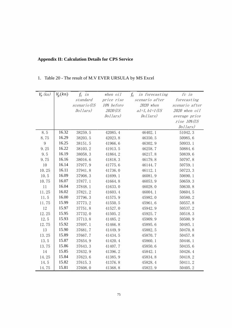
75

Appendix II: Calculation Details for CPS Service

1. Table 20 - The result of M.V EVER URSULA by MS Excel

(kn) ( ) instandard

scenario(USDollars)

when oilprice rise10% before2020(USDollars)

in forecastingscenario after

2020 whena1=1,b1=1(USDollars)

fc inforecasting

scenario after2020 when oilaverage pricerise 10%(USDollars)

8.5 16.32 38259.5 42085.4 46402.1 51042.3

8.75 16.29 38203.5 42023.8 46350.5 50985.6

9 16.25 38151.5 41966.6 46302.9 50933.1

9.25 16.22 38103.2 41913.5 46258.7 50884.6

9.5 16.19 38058.3 41864.2 46217.8 50839.6

9.75 16.16 38016.6 41818.3 46179.8 50797.8

10 16.14 37977.9 41775.6 46144.7 50759.1

10.25 16.11 37941.8 41736.0 46112.1 50723.3

10.5 16.09 37908.3 41699.1 46081.9 50690.1

10.75 16.07 37877.1 41664.8 46053.9 50659.3

11 16.04 37848.1 41633.0 46028.0 50630.8

11.25 16.02 37821.2 41603.4 46004.1 50604.5

11.5 16.00 37796.3 41575.9 45982.0 50580.2

11.75 15.99 37773.2 41550.5 45961.6 50557.8

12 15.97 37751.8 41527.0 45942.9 50537.2

12.25 15.95 37732.0 41505.2 45925.7 50518.3

12.5 15.93 37713.8 41485.2 45909.9 50500.9

12.75 15.92 37697.1 41466.8 45895.6 50485.1

13 15.90 37681.7 41449.9 45882.5 50470.8

13.25 15.89 37667.7 41434.5 45870.7 50457.8

13.5 15.87 37654.9 41420.4 45860.1 50446.1

13.75 15.86 37643.3 41407.7 45850.6 50435.6

14 15.85 37632.9 41396.2 45842.1 50426.4

14.25 15.84 37623.6 41385.9 45834.8 50418.2

14.5 15.82 37615.3 41376.8 45828.4 50411.2

14.75 15.81 37608.0 41368.8 45822.9 50405.2

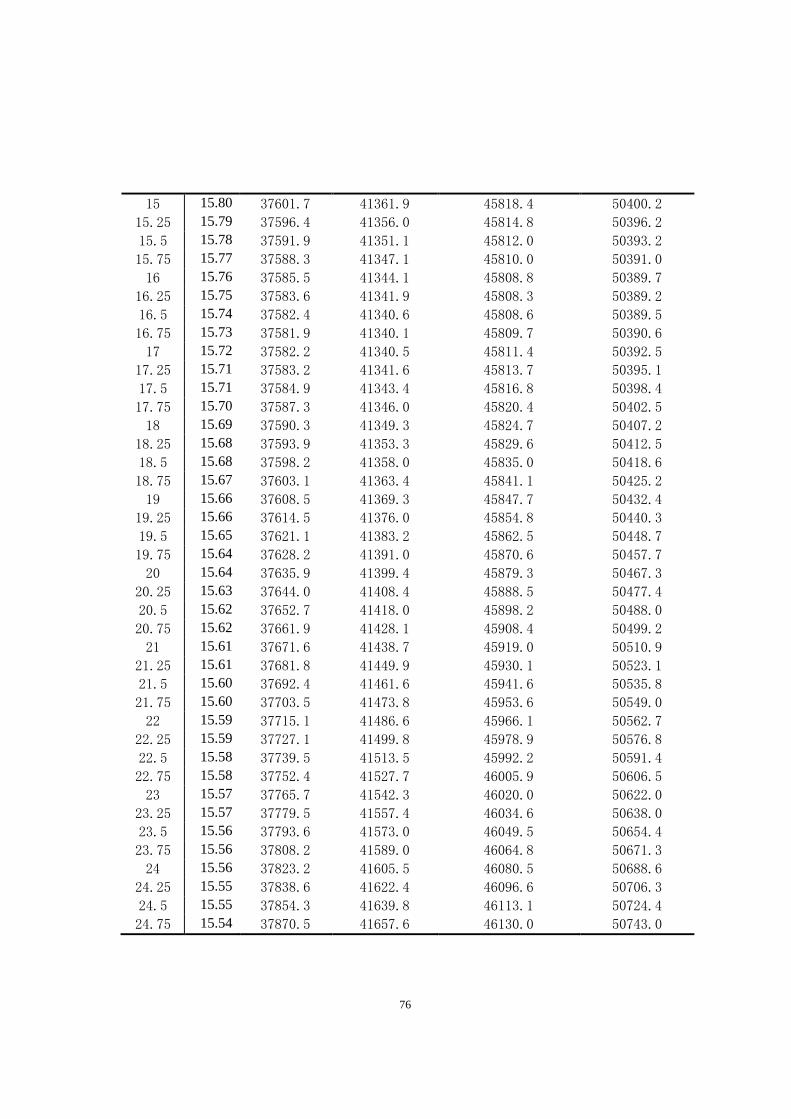
76

15 15.80 37601.7 41361.9 45818.4 50400.2

15.25 15.79 37596.4 41356.0 45814.8 50396.2

15.5 15.78 37591.9 41351.1 45812.0 50393.2

15.75 15.77 37588.3 41347.1 45810.0 50391.0

16 15.76 37585.5 41344.1 45808.8 50389.7

16.25 15.75 37583.6 41341.9 45808.3 50389.2

16.5 15.74 37582.4 41340.6 45808.6 50389.5

16.75 15.73 37581.9 41340.1 45809.7 50390.6

17 15.72 37582.2 41340.5 45811.4 50392.5

17.25 15.71 37583.2 41341.6 45813.7 50395.1

17.5 15.71 37584.9 41343.4 45816.8 50398.4

17.75 15.70 37587.3 41346.0 45820.4 50402.5

18 15.69 37590.3 41349.3 45824.7 50407.2

18.25 15.68 37593.9 41353.3 45829.6 50412.5

18.5 15.68 37598.2 41358.0 45835.0 50418.6

18.75 15.67 37603.1 41363.4 45841.1 50425.2

19 15.66 37608.5 41369.3 45847.7 50432.4

19.25 15.66 37614.5 41376.0 45854.8 50440.3

19.5 15.65 37621.1 41383.2 45862.5 50448.7

19.75 15.64 37628.2 41391.0 45870.6 50457.7

20 15.64 37635.9 41399.4 45879.3 50467.3

20.25 15.63 37644.0 41408.4 45888.5 50477.4

20.5 15.62 37652.7 41418.0 45898.2 50488.0

20.75 15.62 37661.9 41428.1 45908.4 50499.2

21 15.61 37671.6 41438.7 45919.0 50510.9

21.25 15.61 37681.8 41449.9 45930.1 50523.1

21.5 15.60 37692.4 41461.6 45941.6 50535.8

21.75 15.60 37703.5 41473.8 45953.6 50549.0

22 15.59 37715.1 41486.6 45966.1 50562.7

22.25 15.59 37727.1 41499.8 45978.9 50576.8

22.5 15.58 37739.5 41513.5 45992.2 50591.4

22.75 15.58 37752.4 41527.7 46005.9 50606.5

23 15.57 37765.7 41542.3 46020.0 50622.0

23.25 15.57 37779.5 41557.4 46034.6 50638.0

23.5 15.56 37793.6 41573.0 46049.5 50654.4

23.75 15.56 37808.2 41589.0 46064.8 50671.3

24 15.56 37823.2 41605.5 46080.5 50688.6

24.25 15.55 37838.6 41622.4 46096.6 50706.3

24.5 15.55 37854.3 41639.8 46113.1 50724.4

24.75 15.54 37870.5 41657.6 46130.0 50743.0

77

25 15.54 37887.1 41675.8 46147.2 50761.9

25.25 15.54 37904.0 41694.4 46164.8 50781.3

25.5 15.53 37921.3 41713.4 46182.8 50801.0

25.75 15.53 37939.0 41732.9 46201.1 50821.2

26 15.53 37957.0 41752.7 46219.8 50841.8

Source: The author.

2. Table 21- The result of fuel consumption in M.V EVER LOGIC in different

scenarios by MS Excel

(kn) ( ) instandard

scenario(USDollars)

when oilprice rise10% before2020(USDollars)

in forecastingscenario after 2020when a1=1,b1=1(US

Dollars)

fc inforecasting

scenario after2020 when oilaverage pricerise 10%(USDollars)

8.5 16.32 207599 228358.9 254981.7 280479.98.75 16.29 206801.1 227481.2 253956.4 279352.1

9 16.25 206070.6 226677.6 253012.6 278313.99.25 16.22 205402 225942.2 252143.6 277358.09.5 16.19 204790.6 225269.6 251343.4 276477.79.75 16.16 204232 224655.2 250606.8 275667.410 16.14 203722.5 224094.8 249929.0 274921.9

10.25 16.11 203258.8 223584.7 249306.1 274236.710.5 16.09 202837.7 223121.5 248734.1 273607.510.75 16.07 202456.7 222702.3 248209.8 273030.8

11 16.04 202113.1 222324.4 247730.2 272503.211.25 16.02 201804.9 221985.4 247292.5 272021.811.5 16.00 201530.1 221683.1 246894.3 271583.711.75 15.99 201286.8 221415.5 246533.3 271186.7

12 15.97 201073.4 221180.8 246207.6 270828.412.25 15.95 200888.5 220977.3 245915.2 270506.812.5 15.93 200730.6 220803.6 245654.6 270220.112.75 15.92 200598.4 220658.3 245424.1 269966.5

13 15.90 200491 220540.1 245222.4 269744.613.25 15.89 200407.2 220447.9 245048.1 269552.9

78

13.5 15.87 200346.1 220380.7 244900.0 269390.013.75 15.86 200306.7 220337.4 244777.2 269254.9

14 15.85 200288.3 220317.1 244678.5 269146.414.25 15.84 200290.1 220319.2 244603.1 269063.414.5 15.82 200311.5 220342.6 244550.0 269005.014.75 15.81 200351.7 220386.9 244518.5 268970.3

15 15.80 200410.2 220451.3 244507.8 268958.615.25 15.79 200486.5 220535.1 244517.3 268969.115.5 15.78 200580 220638 244546.3 269001.015.75 15.77 200690.2 220759.2 244594.3 269053.7

16 15.76 200816.7 220898.4 244660.6 269126.616.25 15.75 200959.1 221055 244744.7 269219.216.5 15.74 201117 221228.7 244846.2 269330.916.75 15.73 201290 221419.1 244964.7 269461.1

17 15.72 201477.9 221625.7 245099.6 269609.617.25 15.71 201680.2 221848.3 245250.7 269775.817.5 15.71 201896.8 222086.4 245417.5 269959.217.75 15.70 202127.2 222339.9 245599.7 270159.7

18 15.69 202371.3 222608.5 245797.0 270376.718.25 15.68 202628.9 222891.7 246009.0 270609.918.5 15.68 202899.6 223189.5 246235.6 270859.118.75 15.67 203183.3 223501.6 246476.3 271123.9

19 15.66 203479.7 223827.7 246731.0 271404.119.25 15.66 203788.8 224167.7 246999.5 271699.419.5 15.65 204110.2 224521.3 247281.4 272009.519.75 15.64 204443.9 224888.3 247576.6 272334.3

20 15.64 204789.7 225268.7 247885.0 272673.520.25 15.63 205147.4 225662.2 248206.2 273026.820.5 15.62 205516.9 226068.6 248540.1 273394.120.75 15.62 205898.1 226487.9 248886.6 273775.3

21 15.61 206290.8 226919.8 249245.5 274170.121.25 15.61 206694.9 227364.3 249616.7 274578.321.5 15.60 207110.3 227821.3 249999.9 274999.921.75 15.60 207536.9 228290.5 250395.1 275434.6

22 15.59 207974.6 228772 250802.2 275882.422.25 15.59 208423.3 229265.6 251221.0 276343.122.5 15.58 208882.9 229771.2 251651.4 276816.522.75 15.58 209353.3 230288.6 252093.2 277302.6

23 15.57 209834.5 230818 252546.5 277801.223.25 15.57 210326.4 231359 253011.1 278312.223.5 15.56 210828.8 231911.7 253486.9 278835.623.75 15.56 211341.8 232476 253973.8 279371.2

79

24 15.56 211865.3 233051.8 254471.7 279918.924.25 15.55 212399.1 233639.1 254980.6 280478.724.5 15.55 212943.4 234237.7 255500.4 281050.424.75 15.54 213497.9 234847.7 256031.0 281634.1

25 15.54 214062.6 235468.9 256572.3 282229.525.25 15.54 214637.6 236101.3 257124.3 282836.725.5 15.53 215222.7 236744.9 257686.9 283455.625.75 15.53 215817.9 237399.7 258260.0 284086.1

26 15.53 216423.1 238065.4 258843.7 284728.1

Source: The Author.

80

Appendix III: Calculation Details for FAL_1 Service

Table 22- The result of f(v) under the variable of , in a selected vessel of FAL_1service by MS Excel

(kn) (kn) fc in standardscenario(USDollars)

when oil pricerise 10% before2020(USDollars)

fc in forecastingscenario after2020 whena1=1,b1=1 (USDollars)

fc inforecastingscenario after202 when oilaverage pricerise 10%(USDollars)

13.3340 7.5000 143134.8 157448.3 175413.0 192954.313.2745 7.7500 142039.4 156243.3 173987.2 191385.913.2192 8.0000 141065.7 155172.3 172708.2 189979.013.1677 8.2500 140202.2 154222.4 171561.6 188717.813.1195 8.5000 139438.9 153382.8 170535.2 187588.813.0745 8.7500 138767.2 152643.9 169618.3 186580.213.0322 9.0000 138179.5 151997.4 168801.7 185681.812.9924 9.2500 137669.4 151436.3 168077.2 184884.912.9550 9.5000 137231.2 150954.3 167437.8 184181.612.9197 9.7500 136859.8 150545.8 166877.4 183565.112.8863 10.0000 136550.9 150206.0 166390.5 183029.512.8547 10.2500 136300.5 149930.5 165972.1 182569.312.8248 10.5000 136105.2 149715.7 165618.1 182179.912.7964 10.7500 135961.9 149558.0 165324.6 181857.112.7694 11.0000 135867.8 149454.5 165088.2 181597.012.7437 11.2500 135820.4 149402.5 164905.8 181396.412.7192 11.5000 135817.6 149399.4 164774.6 181252.112.6958 11.7500 135857.4 149443.1 164692.2 181161.412.6735 12.0000 135937.9 149531.7 164656.4 181122.012.6522 12.2500 136057.5 149663.3 164665.0 181131.512.6318 12.5000 136214.8 149836.3 164716.4 181188.012.6123 12.7500 136408.4 150049.3 164808.7 181289.612.5936 13.0000 136637.2 150300.9 164940.6 181434.612.5756 13.2500 136900.0 150590.0 165110.5 181621.612.5583 13.5000 137195.8 150915.3 165317.4 181849.112.5418 13.7500 137523.6 151276.0 165559.9 182115.912.5258 14.0000 137882.8 151671.1 165837.2 182420.912.5105 14.2500 138272.4 152099.7 166148.1 182762.912.4957 14.5000 138691.9 152561.1 166491.8 183141.012.4814 14.7500 139140.5 153054.5 166867.5 183554.312.4677 15.0000 139617.6 153579.4 167274.5 184001.9

81

12.4544 15.2500 140122.8 154135.1 167712.0 184483.212.4416 15.5000 140655.5 154721.0 168179.5 184997.412.4292 15.7500 141215.2 155336.7 168676.3 185543.912.4172 16.0000 141801.6 155981.8 169201.9 186122.112.4057 16.2500 142414.2 156655.7 169755.8 186731.412.3945 16.5000 143052.8 157358.0 170337.5 187371.312.3836 16.7500 143716.8 158088.5 170946.7 188041.312.3731 17.0000 144406.2 158846.8 171582.8 188741.112.3629 17.2500 145120.4 159632.5 172245.7 189470.212.3530 17.5000 145859.4 160445.4 172934.8 190228.312.3434 17.7500 146622.9 161285.2 173649.9 191014.912.3434 17.7500 147410.6 162151.7 174390.8 191829.812.3341 18.0000 148222.4 163044.6 175157.0 192672.712.3251 18.2500 149058.0 163963.8 175948.5 193543.312.3163 18.5000 149917.2 164909.0 176764.9 194441.412.3077 18.7500 150800.0 165880.0 177606.0 195366.612.2994 19.0000 151706.2 166876.8 178471.7 196318.912.2914 19.2500 152635.5 167899.1 179361.7 197297.912.2835 19.5000 153588.0 168946.8 180275.9 198303.512.2758 19.7500 154563.5 170019.8 181214.1 199335.512.2684 20.0000 155561.8 171118.0 182176.2 200393.812.2611 20.2500 156582.9 172241.2 183162.0 201478.212.2541 20.5000 157626.7 173389.4 184171.4 202588.612.2472 20.7500 158693.1 174562.4 185204.3 203724.812.2404 21.0000 159782.0 175760.2 186260.6 204886.712.2339 21.2500 160893.4 176982.8 187340.1 206074.212.2275 21.5000 162027.2 178229.9 188442.9 207287.112.2212 21.7500 163183.3 179501.7 189568.7 208525.512.2151 22.0000 164361.7 180797.9 190717.5 209789.312.2092 22.2500 165562.4 182118.6 191889.3 211078.212.2034 22.5000 166785.2 183463.7 193083.9 212392.312.1977 22.7500 168030.2 184833.2 194301.4 213731.612.1921 23.0000 169297.3 186227.1 195541.6 215095.812.1867 23.2500 170586.6 187645.2 196804.6 216485.012.1814 23.5000 171897.9 189087.7 198090.2 217899.212.1762 23.7500 173231.2 190554.3 199398.4 219338.212.1711 24.0000 174586.6 192045.2 200729.2 220802.112.1661 24.2500 175964.0 193560.4 202082.5 222290.812.1613 24.5000 143134.8 157448.3 175413.0 192954.3Source: The author.

82

Appendix IV: Data Resource of the value P/WV

Table 23 - The average global performance of P/WV from 2007 to 2011

Source: IMO(2014). Third IMO GHG study.London: Author.

(Note: The value P/WV is calculated by the Author.)

Average sea

speedAverage P/WV

(knots)

0-999 1015 8976 6004 16.7 178 13.3 0.050293

1000-1999 1142 21644 13153 20 180 15.2 0.03998

2000-2999 684 36869 22228 21.9 178 16.8 0.035886

3000-4999 720 56198 37068 24.7 257 18.6 0.035462

5000-7999 432 79567 58342 26.3 248 20.6 0.035594

8000-11999 135 116415 76214 28.2 249 21.3 0.030736

12000-14500 7 245802 125669 38.4 249 20.6 0.024818

14500-+ 0 0 0 0 0 0 -

0-999 1082 9284 6187 17 178 13.2 0.050486

1000-1999 1253 21824 13367 20.3 179 15.2 0.040295

2000-2999 733 37556 22678 22.3 178 16.7 0.036158

3000-4999 779 56036 37246 24.7 253 18.1 0.036723

5000-7999 472 80503 58986 26.5 246 19.7 0.037194

8000-11999 172 117315 76127 28.4 250 20.3 0.031966

12000-14500 8 163136 83302 25.7 249 19.2 0.026595

14500-+ 0 0 0 0 0 0 -

0-999 1081 9059 6117 16.9 183 13.2 0.051155

1000-1999 1282 21440 13120 20.1 185 15.1 0.040526

2000-2999 752 37550 22613 22.4 217 16.8 0.035846

3000-4999 874 56648 37734 25 238 17.6 0.037847

5000-7999 514 79317 57944 26 266 19.2 0.038049

8000-11999 204 114387 73942 27.3 283 19.9 0.032483

12000-14500 13 187649 91187 29.2 299 17.4 0.027928

14500-+ 0 0 0 0 -

0-999 1023 9080 6182 17.1 191 12.7 0.053609

1000-1999 1264 21520 13156 20.2 201 14.5 0.042161

2000-2999 725 37478 22640 22.4 214 16.2 0.037289

3000-4999 922 58072 39328 25.8 230 17.2 0.039374

5000-7999 564 81168 59115 26.6 228 17.5 0.041617

8000-11999 241 119058 76538 28.3 238 17.9 0.035914

12000-14500 36 283558 131829 43.7 241 17 0.027348

14500-+ 0 0 0 0 0 0 -

0-999 945 9676 5912 16.2 197 12.6 0.048492

1000-1999 1172 20723 12443 19.3 206 14.4 0.041697

2000-2999 666 35764 21668 21.6 222 16 0.037866

3000-4999 864 53951 35980 23.8 241 16.9 0.039462

5000-7999 545 76981 55592 25.2 246 17.2 0.041986

8000-11999 236 108236 68779 25.4 250 17.4 0.03652

12000-14500 47 164333 77563 27.1 240 16.9 0.027928

Average sea

time

2007

2008

2009

2010

2011

yearcapacity

（TEU）

Numbers of

vessel

detectable

by AIS

Average

deadweight

Average

installed

power

Average

designspeed

(knots)