Mathematical

and Computational

Applications

Article

Design Optimization of the Lines of the Bulbous Bowof a Hull Based on Parametric Modeling andComputational Fluid Dynamics Calculation

Weilin Luo 1,2,* and Linqiang Lan 1

1 School of Mechanical Engineering and Automation, Fuzhou University, Fuzhou 350116, China;lanlinqiang@hotmail.com

2 Fujian Province Key Laboratory of Structural Performances in Ship and Ocean Engineering,Fuzhou 350116, China

* Correspondence: wlluo@fzu.edu.cn; Tel.: +86-591-228-64791

Academic Editor: Fazal M. MahomedReceived: 15 August 2016; Accepted: 23 December 2016; Published: 31 December 2016

Abstract: To reduce the ship wave-making resistance, the lines of the bulbous bow of a hull areoptimized by an automatic optimization platform at the ship design stage. Parametric modelingwas applied to the hull by using non-uniform rational basis spline (NURBS). The Rankine-sourcepanel method was used to calculate the wave-making resistance. A hybrid optimization strategywas applied to achieve the optimization goal. A Ro-Ro ship was taken as an example to illustratethe optimization method adopted, with the objective to minimize the wave-making resistance.The optimization results show that wave-making resistance obviously reduces and the wave-shapeof the near bow becomes gentle after the lines of the bulbous bow of the hull are optimized,which demonstrates the validity of the proposed optimization design strategy.

Keywords: hull forms optimization; parametric modeling; computational fluid dynamics calculation;wave-making resistance

1. Introduction

Design of ship hull forms is one of the most important contents of the general ship design.How to reduce the ship resistance by means of well-designed forms is always the concern for shipdesigners and/or researchers. The parent ship based design method predominates in the field ofship design, by which the designed hull can inherit some excellent performance from the parentship. For a long time, designer’s experience played an important role in obtaining the desired hullforms. With the development of computer science and technology, the quality of ship design hasbeen improved considerably by introducing some computational numerical calculation methods.For example, computational fluid dynamics (CFD) based numerical simulation can be used to evaluatethe hydrodynamic performances of a ship after the hull forms are designed. By modifying thehull forms and repeatedly performing CFD simulation, the satisfactory hull forms can be obtained.To improve the design efficiency, computer aided design (CAD) was proposed to combine with CFD inthe optimization design of hull forms [1]. During the past decade, CAD/CFD integrated hull-formdesign systems have been developed and successfully applied to the drag reduction of ships [2].For example, Percival et al. combined a simple CFD tool and B-Spline method to the optimizationdesign of a Wigley ship [3]. Yusuke et al. presented the bulbous bow optimization of a container shipbased on the naval architectural package (NAPA) system and a Rankine-source panel method [1].Tahara et al. applied NAPA and a RANS (Reynolds-averaged Navier–Stokes) solver to the optimizationdesign of a container ship [4]. Abt and Harries presented the generic, multi-objective ship design

Math. Comput. Appl. 2017, 22, 4; doi:10.3390/mca22010004 www.mdpi.com/journal/mca

Math. Comput. Appl. 2017, 22, 4 2 of 12

optimization based on software of the Ship Design Laboratory of the National Technical Universityof Athens (NTUA–SDL) in which well-established naval architectural and optimization softwarepackages are integrated [5]. Harries and Abt distinguished three types of coupling of CAD and CFD [6].Couser et al. explored the multi-dimensional design-space using first-principle methods within theFRIENDSHIP framework [7]. Brizzolara and Vernengo proposed an integration of a parametricgeneration module, a multi-objective optimization algorithm and a CFD solver in the optimization of anew unmanned surface vehicle (USV) and small waterplane area twin hull (SWATH) [8]. Biliotti et al.presented a fully automatic optimization chain to the optimization of fast naval vessels by adoptingthe ModeFrontier optimization environment to the FRIENDSHIP framework, the CFD codes and amulti-objective genetic algorithm [9]. Ginnis et al. employed the NURBS (non-uniform rational basisspline) method and Kelvin-source method to the optimization of a container ship [10]. Brenner etal. used the FRIENDSHIP-SHIPFLOW optimization scheme to retrofit the ships in operation [11].Zakerdoost et al. used the NURBS method and potential theory to the optimization design of a Wigleyship [12]. Vernengo et al. presented the optimization of a Semi-SWATH by a fully parametric model ofthe unconventional hull form, a 3D linear Rankine-sources panel method, and a multiobjective globalconvergence genetic algorithm [13]. Combined with the optimization of a high speed round bilgemonohull, Brizzolara et al. addressed the significance of parametric hull form definition by comparingit with Free Form Deformation technique [14]. Ang et al. proposed the Free Form Deformation andpotential theory to the optimization design of a heavy-lift and pipe-lay vessel [15]. Wang proposed theNURBS method and CFD calculation based on Neumann–Michell theory to the optimization design ofseveral life ships [16].

Besides the parametric modeling of hull forms and calculation of hydrodynamic performances,optimization is another important factor in the hull-form design system. To guarantee the optimumdesign and the solving efficiency, an appropriate optimization algorithm is vital to the optimizer.During the last several decades, many optimization algorithms have been proposed such as successivequadratic programming (SQP) [17], genetic algorithm (GA) [18], simulated annealing (SA) [19],particle swarm optimization (PSO) [20], infeasibility driven evolutionary algorithm (IDEA) [21],and quasi-Newton method [10], among others. Generally, these algorithms can be categorized intogradient-based and derivative-free methods [22]. For the gradient-based optimization algorithms(e.g., SQP and quasi-Newton approaches), the interest is the fast convergence; however, the limitationis the locally optimal solution. For the derivative-free optimization algorithms (e.g., GA, SA, PSO,and IDEA approaches), the advantage is the global optimization; however, the convergence rate cannotbe guaranteed. Since each optimization algorithm has its advantages and disadvantages, a hybridoptimization scheme should be preferable. In this paper, we perform the combination of a globaloptimization method (Ensemble Investigation) and a local optimization method (T-Search algorithm)to the optimization design of hull forms of a surface ship. The design optimization is carried outin the SHIPFLOW-CAESES (former FRIENDSHIP) DESIGN environment. Based on the automaticoptimization platform, the parametric modeling and the CFD calculation are integrated. The NURBSmethod is employed to the parametric modeling while the Rankine-source panel method is applied tocalculate the wave-making resistance. The minimization of the wave-making resistance is taken as theoptimization objective while the design variables are form parameters of the lines of the bulbous bow.

The rest of the paper is organized as follows. In Section 2, the parametric modeling methodis introduced; in Section 3, the CFD method to calculate the wave-making resistance is described;in Section 4, the hybrid optimization algorithm is addressed; in Section 5, the entire optimizationscheme is described; in Section 6, an example is studied to confirm the validity of the optimizationstrategy proposed in the study; and the final section is the concluding remarks.

2. Parametric Modeling of Hull Forms

In the geometry modeling of a hull, it is often required to obtain the forms rapidly. In addition,a large number of forms should be analyzed so that the optimization can be efficiently performed.

Math. Comput. Appl. 2017, 22, 4 3 of 12

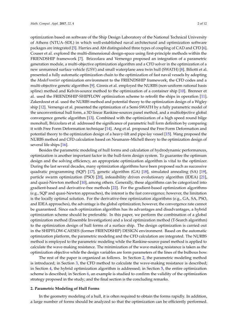
In this paper, the NURBS method is employed to meet the mentioned requirements. Based onthis method, the high-quality of the lines can be guaranteed with fairly less design variables thanconventional design methodology. This method provides the best way to establish the relationshipbetween parameters and hull forms and makes sure that the design variation among the entireoptimization process is effective and feasible. The parametric model is generated by CAESES-Modeler.The process of curves generation starts with a set of given data elements that are used to definethe complete parametric curve. Within the modeler, one can define a set of longitudinal lines andexpress them as basic curves to describe the ship hull by means of differential, integral and topologicalinformation. Transversal basic curves are able to be formed as soon as the longitudinal basic curvesare defined (by fair B-Spline parametric curves adopted in the study). Then, a series of surfaces canbe set up by corresponding transversal sections that stem from the parametric hull model. Generally,the design of the fully parametric hull surfaces makes it possible to transform the hull form efficientlyand effectively. Moreover, all of the hull topologies, the hull sections and the whole hull surface can begenerated using the basic curves specifically and precisely. Usually, the hull forms are described byfeature curves [23], e.g., the design waterline, flat of side, flat of bottom, etc., which are listed in Table 1and some of the curves are shown in Figure 1.

Table 1. Basic feature curves describing hull forms.

Characteristic Curve Abbreviation

Position Design waterline DWLDeck line DEC

Flat of side curve FOSFlat of bottom curve FOBCenter plane curve CPC

Tangent angle Tangent angle at beginning and end TAB, TAECurvature Curvature at beginning and end CAB,CAE

Area Sectional area curve SACCentroid of area Vertical and Lateral moments of sectional area VMS, LMS

Math. Comput. Appl. 2017, 22, 4  3 of 12 

conventional design methodology. This method provides the best way to establish the relationship 

between parameters  and hull  forms  and makes  sure  that  the design  variation  among  the  entire 

optimization  process  is  effective  and  feasible.  The  parametric model  is  generated  by  CAESES‐

Modeler. The process of curves generation starts with a set of given data elements that are used to 

define the complete parametric curve. Within the modeler, one can define a set of longitudinal lines 

and express  them as basic  curves  to describe  the  ship hull by means of differential,  integral and 

topological information. Transversal basic curves are able to be formed as soon as the longitudinal 

basic curves are defined (by fair B‐Spline parametric curves adopted in the study). Then, a series of 

surfaces can be set up by corresponding transversal sections that stem from the parametric hull model. 

Generally,  the design of  the  fully parametric hull surfaces makes  it possible  to  transform  the hull 

form efficiently and effectively. Moreover, all of the hull topologies, the hull sections and the whole 

hull surface can be generated using the basic curves specifically and precisely. Usually, the hull forms 

are described by feature curves [23], e.g., the design waterline, flat of side, flat of bottom, etc., which 

are listed in Table 1 and some of the curves are shown in Figure 1. 

Table 1. Basic feature curves describing hull forms 

Characteristic  Curve Abbreviation 

Position  Design waterline  DWL 

  Deck line  DEC 

  Flat of side curve  FOS 

  Flat of bottom curve  FOB 

  Center plane curve  CPC 

Tangent angle  Tangent angle at beginning and end  TAB, TAE 

Curvature  Curvature at beginning and end  CAB,CAE 

Area  Sectional area curve  SAC 

Centroid of area  Vertical and Lateral moments of sectional area  VMS, LMS 

 

Figure 1. Basic feature curves describing hull forms. 

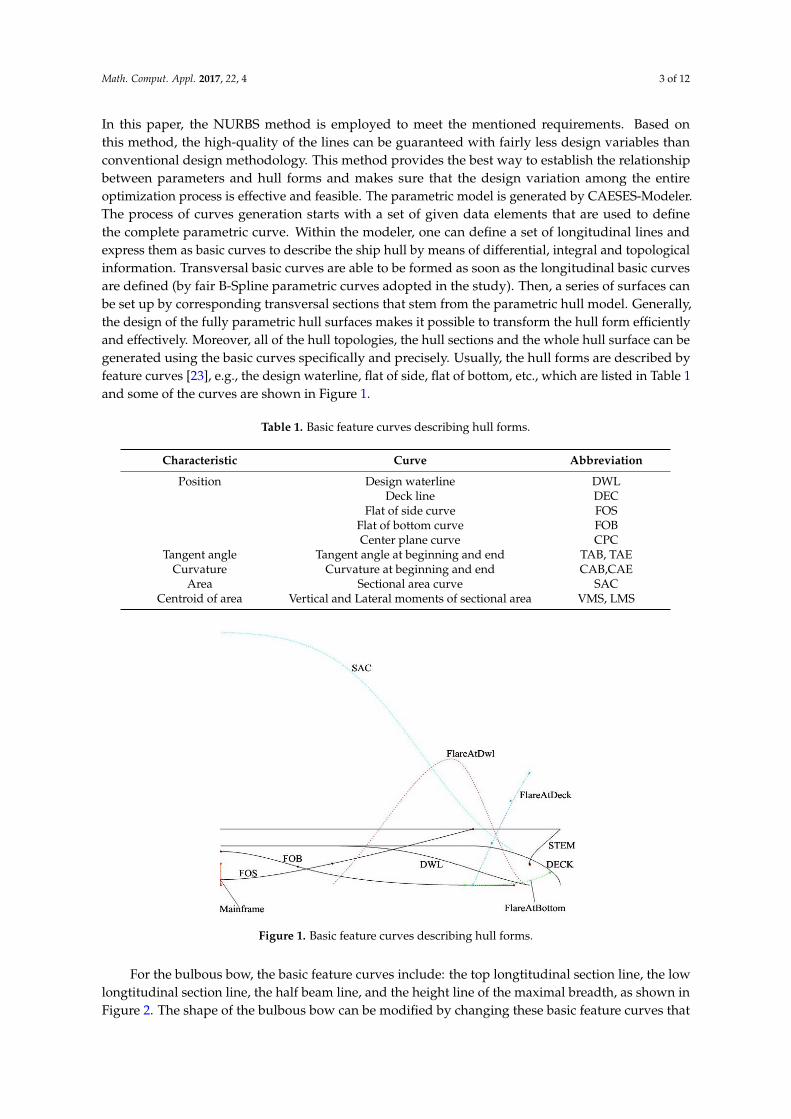
For the bulbous bow, the basic feature curves include: the top longtitudinal section line, the low 

longtitudinal section line, the half beam line, and the height line of the maximal breadth, as shown in 

Figure 2. The shape of the bulbous bow can be modified by changing these basic feature curves that 

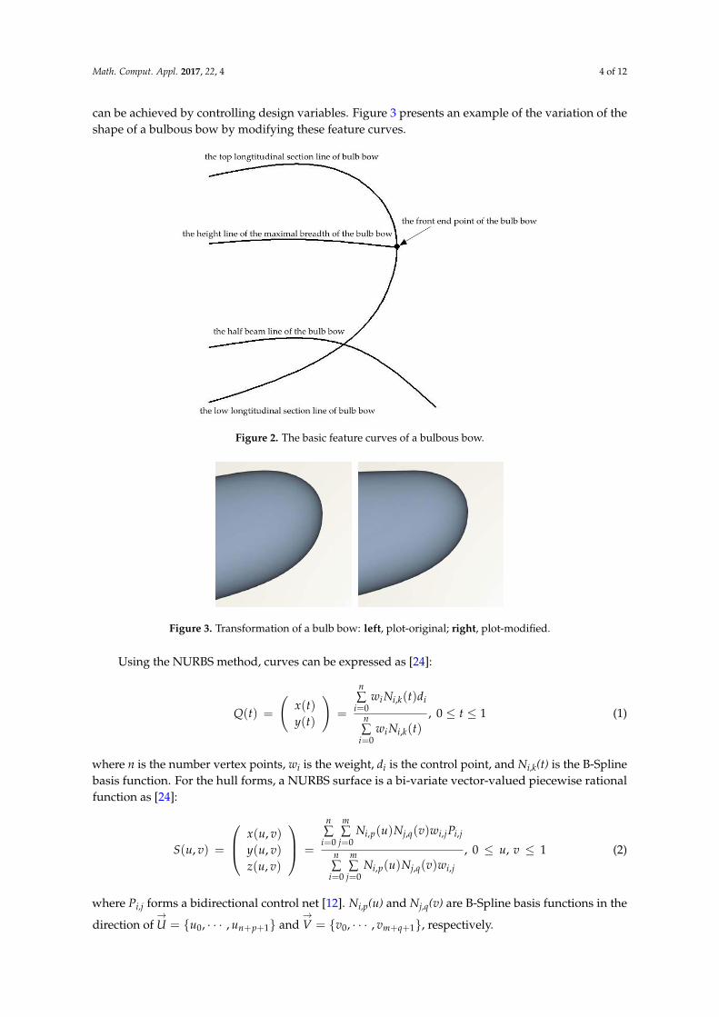
can be achieved by controlling design variables. Figure 3 presents an example of the variation of the 

shape of a bulbous bow by modifying these feature curves. 

Figure 1. Basic feature curves describing hull forms.

For the bulbous bow, the basic feature curves include: the top longtitudinal section line, the lowlongtitudinal section line, the half beam line, and the height line of the maximal breadth, as shown inFigure 2. The shape of the bulbous bow can be modified by changing these basic feature curves that

Math. Comput. Appl. 2017, 22, 4 4 of 12

can be achieved by controlling design variables. Figure 3 presents an example of the variation of theshape of a bulbous bow by modifying these feature curves.Math. Comput. Appl. 2017, 22, 4  4 of 12 

 

Figure 2. The basic feature curves of a bulbous bow 

   

Figure 3. Transformation of a bulb bow: left, plot‐original; right, plot‐modified 

Using the NURBS method, curves can be expressed as [24]: 

,0

,0

( )( )

( ) , 0 1( )

( )

n

i i k ii

n

i i ki

w N t dx t

Q t ty t

w N t

  (1) 

where n is the number vertex points, wi is the weight, di is the control point, and Ni,k(t) is the B‐Spline basis function. For the hull forms, a NURBS surface is a bi‐variate vector‐valued piecewise rational 

function as [24]: 

, , , ,0 0

, , ,0 0

( ) ( ) ( )

( , ) ( ) , 0 , 1( ) ( )( )

n m

i p j q i j i ji j

n m

i p j q i ji j

x u,v N u N v w P

S u v y u,v u vN u N v wz u,v

  (2) 

where Pi,j forms a bidirectional control net [12]. Ni,p(u) and Nj,q(v) are B‐Spline basis functions in the 

direction of  0 1{ , , }n pU u u

and  0 1{ , , }m qV v v

, respectively. 

The hull forms can be expressed parametrically by using the form parameters to constitute the 

feature curves and hull section frames. The general procedure to generate fairing surfaces of the hull 

Figure 2. The basic feature curves of a bulbous bow.

Math. Comput. Appl. 2017, 22, 4  4 of 12 

 

Figure 2. The basic feature curves of a bulbous bow 

   

Figure 3. Transformation of a bulb bow: left, plot‐original; right, plot‐modified 

Using the NURBS method, curves can be expressed as [24]: 

,0

,0

( )( )

( ) , 0 1( )

( )

n

i i k ii

n

i i ki

w N t dx t

Q t ty t

w N t

  (1) 

where n is the number vertex points, wi is the weight, di is the control point, and Ni,k(t) is the B‐Spline basis function. For the hull forms, a NURBS surface is a bi‐variate vector‐valued piecewise rational 

function as [24]: 

, , , ,0 0

, , ,0 0

( ) ( ) ( )

( , ) ( ) , 0 , 1( ) ( )( )

n m

i p j q i j i ji j

n m

i p j q i ji j

x u,v N u N v w P

S u v y u,v u vN u N v wz u,v

  (2) 

where Pi,j forms a bidirectional control net [12]. Ni,p(u) and Nj,q(v) are B‐Spline basis functions in the 

direction of  0 1{ , , }n pU u u

and  0 1{ , , }m qV v v

, respectively. 

The hull forms can be expressed parametrically by using the form parameters to constitute the 

feature curves and hull section frames. The general procedure to generate fairing surfaces of the hull 

Figure 3. Transformation of a bulb bow: left, plot-original; right, plot-modified.

Using the NURBS method, curves can be expressed as [24]:

Q(t) =

(x(t)y(t)

)=

n∑

i=0wi Ni,k(t)di

n∑

i=0wi Ni,k(t)

, 0 ≤ t ≤ 1 (1)

where n is the number vertex points, wi is the weight, di is the control point, and Ni,k(t) is the B-Splinebasis function. For the hull forms, a NURBS surface is a bi-variate vector-valued piecewise rationalfunction as [24]:

S(u, v) =

x(u, v)y(u, v)z(u, v)

=

n∑

i=0

m∑

j=0Ni,p(u)Nj,q(v)wi,jPi,j

n∑

i=0

m∑

j=0Ni,p(u)Nj,q(v)wi,j

, 0 ≤ u, v ≤ 1 (2)

where Pi,j forms a bidirectional control net [12]. Ni,p(u) and Nj,q(v) are B-Spline basis functions in the

direction of→U = {u0, · · · , un+p+1} and

→V = {v0, · · · , vm+q+1}, respectively.

Math. Comput. Appl. 2017, 22, 4 5 of 12

The hull forms can be expressed parametrically by using the form parameters to constitutethe feature curves and hull section frames. The general procedure to generate fairing surfaces ofthe hull form observes four steps, as presented in Figure 4. First, the form parameters should besuitably selected. Second, the parametric design of the longitudinal feature curves is performed. Third,transversal feature curves can be similarly generated and a set of surfaces can be derived by means ofinterpolation. Finally, fairing form variations can be obtained [23]. It should be noted that the numberand the range of the form parameters should be selected carefully to prevent any distortion of the ship.In the study, eight form parameters are selected for the generation of the bulbous bow. More detailsabout these parameters are presented in the Example Study section.

Math. Comput. Appl. 2017, 22, 4 5 of 12

form observes four steps, as presented in Figure 4. First, the form parameters should be suitably selected. Second, the parametric design of the longitudinal feature curves is performed. Third, transversal feature curves can be similarly generated and a set of surfaces can be derived by means of interpolation. Finally, fairing form variations can be obtained [23]. It should be noted that the number and the range of the form parameters should be selected carefully to prevent any distortion of the ship. In the study, eight form parameters are selected for the generation of the bulbous bow. More details about these parameters are presented in the Example Study section.

Figure 4. Parametric modeling of a hull form.

3. Calculation of Wave-Making Resistance

In the study, the optimization objective is to minimize the wave-making resistance. Suppose the fluid is inviscid and incompressible, and Rankine-source panel method is employed.

For a ship traveling with a steady forward speed U in the calm water of infinite depth, the wave-making velocity potential ϕ(x,y,z) satisfies the following equations:

in the fluid domain: 2 0φ∇ = (3)

on the free surface: 1 1

2sUgξ φ φ φ = − ⋅∇ + ∇ ⋅∇

(4)

on the free surface: ( )s zU nφ ξ φ∇ − ⋅ ⋅∇ =

(5)

on the hull surface: sU nnφ∂ = ⋅

∂

(6)

at infinity: ( )0,0,0φ∇ = (7)

where ( ),0,0sU U= , g is the acceleration of gravity, and ξ is the free surface elevation.

The velocity potential at the field point P can be calculated as [25]

( ) ( ) ( ) ( ) ( ) ( ) ( )1 1 1 1 1 1

4 , , 4 , ,SB SFP Q ds Q ds

r P Q r P Q r P Q r P Qφ σ σ

π π

= − + − + ′ ′ ′ ′

(8)

where Q and Q’ are source points, σ(Q) is the source strength, and r and r’ are the distances between the field point and source points.

When the ship is sailing, the wave is steep and the floating state cannot be neglected. Therefore, the nonlinear free surface boundary condition should be used. The method of Taylor series expansion is applied to Equations (4) and (5) by making use of the approximate solution z = Z and ϕ = φ. Then, the boundary condition on the approximate free surface can be obtained as:

( ) ( ) [ ] ( )1 12 2zA U WB W W g A U B A gZϕ φ ϕ φ ϕ ϕ ∇ − ∇ + ⋅∇ + ⋅ ⋅∇ ∇ + = ∇ ⋅ ∇ − ∇ + −

(9)

z

W A gZZW g

φξϕ

⋅∇ − += +⋅∇ −

(10)

Selection of form

parameters

Longitudinal

feature curves

Transversal

feature curves

Fairing form

surfaces

Figure 4. Parametric modeling of a hull form.

3. Calculation of Wave-Making Resistance

In the study, the optimization objective is to minimize the wave-making resistance. Suppose thefluid is inviscid and incompressible, and Rankine-source panel method is employed.

For a ship traveling with a steady forward speed U in the calm water of infinite depth, thewave-making velocity potential ϕ(x,y,z) satisfies the following equations:

in the fluid domain : ∇2φ = 0 (3)

on the free surface : =1g

(−Us · ∇φ +

12∇φ · ∇φ

)(4)

on the free surface :(∇φ − Us ·

→n)· ∇ξ = φz (5)

on the hull surface :∂φ

∂n= Us ·

→n (6)

at infinity : ∇φ = (0, 0, 0) (7)

where Us = (U, 0, 0), g is the acceleration of gravity, and ξ is the free surface elevation.The velocity potential at the field point P can be calculated as [25]

φ(P) = − 14π

x

SB

σ(Q)

(1

r(P, Q)+

1r′(P, Q′)

)ds − 1

4π

x

SF

σ(Q)

(1

r(P, Q)+

1r′(P, Q′)

)ds (8)

where Q and Q’ are source points, σ(Q) is the source strength, and r and r’ are the distances betweenthe field point and source points.

When the ship is sailing, the wave is steep and the floating state cannot be neglected. Therefore,the nonlinear free surface boundary condition should be used. The method of Taylor series expansionis applied to Equations (4) and (5) by making use of the approximate solution z = Z and ϕ = φ. Then,the boundary condition on the approximate free surface can be obtained as:

[2(∇A − U∇ϕ1) +

→WB

]· ∇φ +

→W ·

[(→W · ∇

)∇ϕ

]+ gφz = 2∇ϕ · [∇A − U∇ϕ1] + B(A − gZ) (9)

ξ = Z +

→W · ∇φ − A + gZ→W · ∇ϕz − g

(10)

Math. Comput. Appl. 2017, 22, 4 6 of 12

where→W = ∇φ − Us, A = 1

2∇ϕ · ∇ϕ and B =

[→W·(∇A−U∇ϕx) + gϕz

]z

→W·∇ϕz − g

.

The boundary condition on the ship surface is:

∇φ ·→n = Un1 (11)

Based on Bernoulli equation, the pressure can be calculated as

p = ρ(Uφx − (∇φ · ∇φ)/2 + gz) (12)

where U is the ship velocity, and ρ is the fluid density. By integrating the pressure along the wettedboundary surface, one has the hydrodynamic force on the hull as

→F = (F1, F2, F3) =

x

SB

p→n dS (13)

Thus, the wave-making resistance and its nondimensional form can be obtained as

Rw = −F1 = −x

SB

pn1dS (14)

andCw =

Rw

0.5ρU2S0(15)

respectively, where S0 is the wetted surface area in calm waters. Cw is also named as the coefficient ofwave-making resistance.

4. Optimization Algorithms

To guarantee the globally optimal solution and solving efficiency as well, a hybrid algorithmis applied in the study. Ensemble Investigation is employed to obtain the globally optimal solution.This algorithm allows permuting a set of design variables and generating DOE (design of experiments)tables, which is very effective to gather information about the optimization problem investigated in thewhole design space. Generated DOE tables are useful to detect the trends of the optimization variableswith regard to the optimization objectives, irrespective of constraints [26]. This optimization approachis performed by creating several different versions of a proposed new design, and then selecting theoption that best fits the design goals. The generation of a systematic series of design options canbe completed soon. These options are tested against design goals—for example, the hydrodynamicperformance. Computational techniques such as regression analysis can be used to determine the“best” option.

To improve the efficiency of solution-searching, the T-Search algorithm is incorporated.This algorithm is a method of feasible direction. It uses a direct search until some constraint getsviolated. At the expense of a little extra effort, T-Search is characterized by efficient operation withinthe admissible region with satisfactory performance along the boundary of that region [27]. The othertwo features of the algorithm are the allowance made for small perturbations of the base point andthe flexible directions for exploration in the tangent hyperspace [28]. It consists of exploratory movesthat start from a so-called base point along the variable axes followed by global moves in the descentsearch direction found in successful exploratory moves. If a constraint bound is approached, then itreturns to the last admissible point and performs a unidirectional optimization along the hyperplanetangent to the active constraint either to keep the search in the feasible domain or to bring it back to thefeasible domain. T-Search is able to find the local minimum of an arbitrary, explicitly-stated functionof more than one variable, subject to arbitrary, non-linear constraints.

Math. Comput. Appl. 2017, 22, 4 7 of 12

5. Optimization Scheme

5.1. Optimization Goal and Design Variables

The optimization objective in the study is to minimize the wave-making resistance under designedship velocity, i.e., min{Cw}. The constraints are set to be subject to (1) |∆0 − ∆p|/∆0 ≤ 1% where ∆0 isthe initial displacement, and ∆p is the displacement of optimized ship; (2) |LCB0 − LCBp|/LCB0 ≤ 1%,where LCB0 is the initial longitudal coordiante of the boyance center while LCBp is the longitudalcoordiante of boyance center of the optimized ship; and (3) the ship length, breadth and draft areconstant during the optimization process.

Since the lines of the bulbous bow are vital to the wave-making resistance, the design variablesare selected as form control parameters of bulbous bow, including the distance between the centerof the bulb bow and the front end of the bulb bow (Dcf); the height of the front end of the bulb bow(Hf); the contour fullness of the top longtitudinal section of bulb bow (Ftl) and its coefficient (Cftl);the contour fullness of the low longtitudinal section of bulb bow (Fll) and its coefficient (Cfll);the contour fullness at the half beam of the bulb bow (Fhb); and half of the maximal breadth ofthe bulb bow (Bh). These form control parameters are used to generate the basic feature curves of thebulbous bow, as shown in Figure 2.

5.2. Optimization Framework

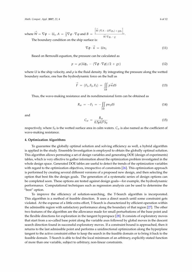
In the optimization framework, there are mainly three modules: the parametric modeling,CFD calculation and lines modification. The optimization operation is performed in theSHIPFLOW-CAESES DESIGN environment. First, NURBS based parametric modeling is performedin the CAESES and the lines offsets of the given hull can be obtained. Then, the files of the lines ofoffsets are automatically imported into the SHIPFLOW so that the CFD calculation can be carried out.Afterwards, the CFD results are imported to CAESES as comparison with the optimization objective.If the optimization goal is achieved, the lines are exported as the optimal lines; otherwise, the designvariables are modified based on the hybrid optimization algorithm, and the optimization operation isrepeated until the optimization goal is achieved. For general procedure, the optimization design ispresented in Figure 5.

Math. Comput. Appl. 2017, 22, 4 7 of 12

The optimization objective in the study is to minimize the wave-making resistance under designed ship velocity, i.e., min{Cw}. The constraints are set to be subject to (1) |Δ0 − Δp|/Δ0 ≤ 1% where Δ0 is the initial displacement, and Δp is the displacement of optimized ship; (2) |LCB0 − LCBp|/LCB0 ≤ 1%, where LCB0 is the initial longitudal coordiante of the boyance center while LCBp is the longitudal coordiante of boyance center of the optimized ship; and (3) the ship length, breadth and draft are constant during the optimization process.

Since the lines of the bulbous bow are vital to the wave-making resistance, the design variables are selected as form control parameters of bulbous bow, including the distance between the center of the bulb bow and the front end of the bulb bow (Dcf); the height of the front end of the bulb bow (Hf); the contour fullness of the top longtitudinal section of bulb bow (Ftl) and its coefficient (Cftl); the contour fullness of the low longtitudinal section of bulb bow (Fll) and its coefficient (Cfll); the contour fullness at the half beam of the bulb bow (Fhb); and half of the maximal breadth of the bulb bow (Bh). These form control parameters are used to generate the basic feature curves of the bulbous bow, as shown in Figure 2.

5.2. Optimization Framework

In the optimization framework, there are mainly three modules: the parametric modeling, CFD calculation and lines modification. The optimization operation is performed in the SHIPFLOW-CAESES DESIGN environment. First, NURBS based parametric modeling is performed in the CAESES and the lines offsets of the given hull can be obtained. Then, the files of the lines of offsets are automatically imported into the SHIPFLOW so that the CFD calculation can be carried out. Afterwards, the CFD results are imported to CAESES as comparison with the optimization objective. If the optimization goal is achieved, the lines are exported as the optimal lines; otherwise, the design variables are modified based on the hybrid optimization algorithm, and the optimization operation is repeated until the optimization goal is achieved. For general procedure, the optimization design is presented in Figure 5.

It is noted that a batch file is necessary to connect SHIPFLOW and CAESES applications. SHIPFLOW provides the batch file in the installation package. The batch file includes echo commands, pause commands, call commands, start commands, go-to commands, and set commands. There is a boundary of surface between the surface of the bulbous bow and the surface of the front part of hull. This boundary is maintained between optimization circles so that the bulbous bow can connect to the front part of hull smoothly.

Figure 5. Optimization procedure.

Parametric modeling

Files of lines offsets

CFD calculation

Output CFD results

Optimization goal achieved?

Optimal lines

Modify design variables

Yes

No

Figure 5. Optimization procedure.

Math. Comput. Appl. 2017, 22, 4 8 of 12

It is noted that a batch file is necessary to connect SHIPFLOW and CAESES applications.SHIPFLOW provides the batch file in the installation package. The batch file includes echo commands,pause commands, call commands, start commands, go-to commands, and set commands. There is aboundary of surface between the surface of the bulbous bow and the surface of the front part of hull.This boundary is maintained between optimization circles so that the bulbous bow can connect to thefront part of hull smoothly.

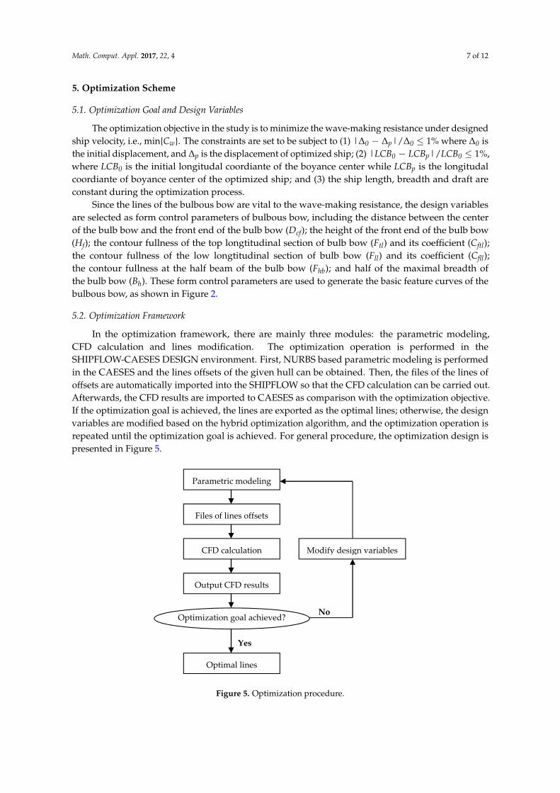
6. Example Study

A Ro-Ro ship is investigated to verify the optimization scheme proposed in the study. The mainparticulars of the ship are listed in Table 2. The ship velocity is 22 knots. In terms of Froude number,one has Fr = 0.28.

Table 2. Main particulars of a Ro-Ro ship.

Description Variable Value

Length (m) L 165Breadth (m) B 24.8

Draft (m) d 8.7Block coefficient Cb 0.65

In the CAESES framework, the form parameters are imported to the curve generator to obtain aset of feature curves. Then, fairing surfaces can be derived automatically through a surface generator.The parameterized hull surfaces are shown in Figure 6.

Math. Comput. Appl. 2017, 22, 4 8 of 12

6. Example Study

A Ro-Ro ship is investigated to verify the optimization scheme proposed in the study. The main particulars of the ship are listed in Table 2. The ship velocity is 22 knots. In terms of Froude number, one has Fr = 0.28.

Table 2. Main particulars of a Ro-Ro ship.

Description Variable ValueLength (m) L 165 Breadth (m) B 24.8

Draft (m) d 8.7 Block coefficient Cb 0.65

In the CAESES framework, the form parameters are imported to the curve generator to obtain a set of feature curves. Then, fairing surfaces can be derived automatically through a surface generator. The parameterized hull surfaces are shown in Figure 6.

Figure 6. Hull surfaces of the Ro-Ro ship.

Based on the optimization framework shown in Figure 5, the hybrid optimization algorithm is performed. In detail, the Ensemble Investigation is employed to obtain feasible solutions in the whole design space. A set of optimized hull forms that satisfy the constraints are derived. Then, the T-Search algorithm is used within the set to determine the solution with minimal wave-making resistance. The design variables and their variations are listed in Table 3. The results of optimization objective and constraints are presented in Table 4.

Table 3. Optimization results of the design variables.

Design Variable Range Initial Value Optimized Value Dcf (m) [0, 1] 0.624 0.237 Hf (m) [1, 5.5] 4.287 4.856

Ftl [0.1, 0.6] 0.41 0.34 Cftl [0.52, 0.91] 0.73 0.842 Fll [1.12, 1.37] 1.28 1.31 Cfll [0.65, 0.96] 0.85 0.943 Fhb [1.4, 2.0] 1.64 1.873

Bh (m) [2.1, 2.58] 2.301 2.384 Dcf, the distance between the center of the bulb bow and the front end of the bulb bow; Hf, the height of the front end of the bulb bow; Ftl, the contour fullness of the top longtitudinal section of the bulb bow; Cftl, the coefficient of the contour fullness of the top longtitudinal section; Fll, the contour fullness of the low longtitudinal section of the bulb bow; Cfll, the coefficient of the contour fullness of the low

Figure 6. Hull surfaces of the Ro-Ro ship.

Based on the optimization framework shown in Figure 5, the hybrid optimization algorithm isperformed. In detail, the Ensemble Investigation is employed to obtain feasible solutions in the wholedesign space. A set of optimized hull forms that satisfy the constraints are derived. Then, the T-Searchalgorithm is used within the set to determine the solution with minimal wave-making resistance.The design variables and their variations are listed in Table 3. The results of optimization objective andconstraints are presented in Table 4.

Math. Comput. Appl. 2017, 22, 4 9 of 12

Table 3. Optimization results of the design variables.

Design Variable Range Initial Value Optimized Value

Dcf (m) [0, 1] 0.624 0.237Hf (m) [1, 5.5] 4.287 4.856

Ftl [0.1, 0.6] 0.41 0.34Cftl [0.52, 0.91] 0.73 0.842Fll [1.12, 1.37] 1.28 1.31Cfll [0.65, 0.96] 0.85 0.943Fhb [1.4, 2.0] 1.64 1.873

Bh (m) [2.1, 2.58] 2.301 2.384

Dcf, the distance between the center of the bulb bow and the front end of the bulb bow; Hf, the height of the frontend of the bulb bow; Ftl, the contour fullness of the top longtitudinal section of the bulb bow; Cftl, the coefficientof the contour fullness of the top longtitudinal section; Fll, the contour fullness of the low longtitudinal sectionof the bulb bow; Cfll, the coefficient of the contour fullness of the low longtitudinal section; Fhb, the contourfullness at the half beam of the bulb bow; Bh, half of the maximal breadth of the bulb bow.

Table 4. Optimization results of the objective and constraints.

Description Initial Value Optimized Value Variation

Nondimensional wave-making resistance, Cw 0.0020368 0.0019488 4.32% (↓)Displacement, ∆(t) 22357.695 22382.706 0.112% (↑)

Longitudal coordiante of boyance center, LCB (m) 0.515798 0.515262 0.104% (↓)

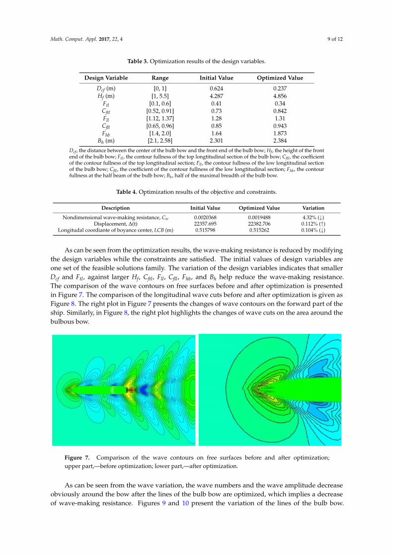
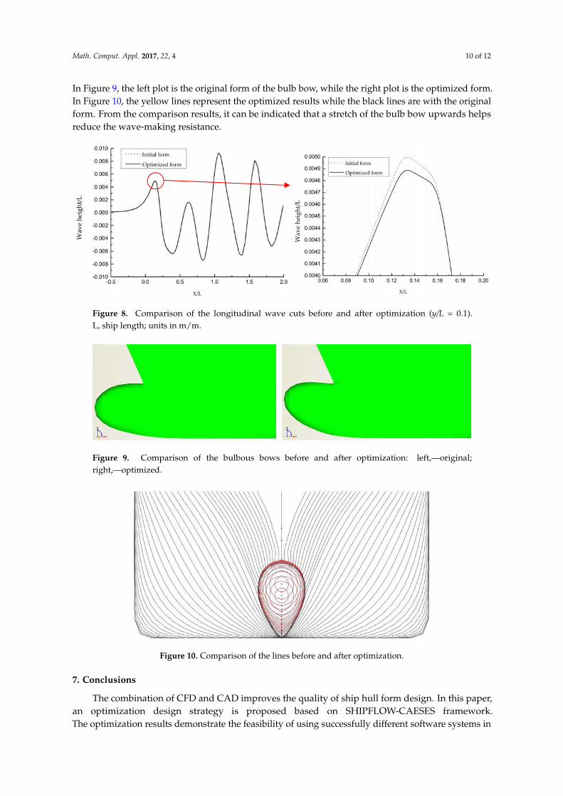
As can be seen from the optimization results, the wave-making resistance is reduced by modifyingthe design variables while the constraints are satisfied. The initial values of design variables areone set of the feasible solutions family. The variation of the design variables indicates that smallerDcf and Ftl, against larger Hf, Cftl, Fll, Cfll, Fhb, and Bh help reduce the wave-making resistance.The comparison of the wave contours on free surfaces before and after optimization is presentedin Figure 7. The comparison of the longitudinal wave cuts before and after optimization is given asFigure 8. The right plot in Figure 7 presents the changes of wave contours on the forward part of theship. Similarly, in Figure 8, the right plot highlights the changes of wave cuts on the area around thebulbous bow.

Math. Comput. Appl. 2017, 22, 4  9 of 12 

longtitudinal section; Fhb, the contour fullness at the half beam of the bulb bow; Bh, half of the maximal 

breadth of the bulb bow. 

Table 4. Optimization results of the objective and constraints. 

Description  Initial Value Optimized Value  Variation 

Nondimensional wave‐making 

resistance, Cw 0.0020368  0.0019488  4.32% (↓) 

Displacement, Δ(t)  22357.695  22382.706  0.112% (↑) Longitudal coordiante of boyance 

center, LCB (m) 0.515798  0.515262  0.104% (↓) 

As  can  be  seen  from  the  optimization  results,  the  wave‐making  resistance  is  reduced  by 

modifying  the  design  variables while  the  constraints  are  satisfied.  The  initial  values  of  design 

variables are one set of the feasible solutions family. The variation of the design variables indicates 

that smaller Dcf and Ftl, against larger Hf, Cftl, Fll, Cfll, Fhb, and Bh help reduce the wave‐making resistance. 

The comparison of the wave contours on free surfaces before and after optimization is presented in 

Figure 7. The comparison of  the  longitudinal wave cuts before and after optimization  is given as 

Figure 8. The right plot in Figure 7 presents the changes of wave contours on the forward part of the 

ship. Similarly, in Figure 8, the right plot highlights the changes of wave cuts on the area around the 

bulbous bow. 

   

Figure 7. Comparison of  the wave contours on  free surfaces before and after optimization; upper 

part,—before optimization; lower part,—after optimization. 

 Figure 8. Comparison of the longitudinal wave cuts before and after optimization (y/L = 0.1). L, ship 

length; units in m/m. 

Figure 7. Comparison of the wave contours on free surfaces before and after optimization;upper part,—before optimization; lower part,—after optimization.

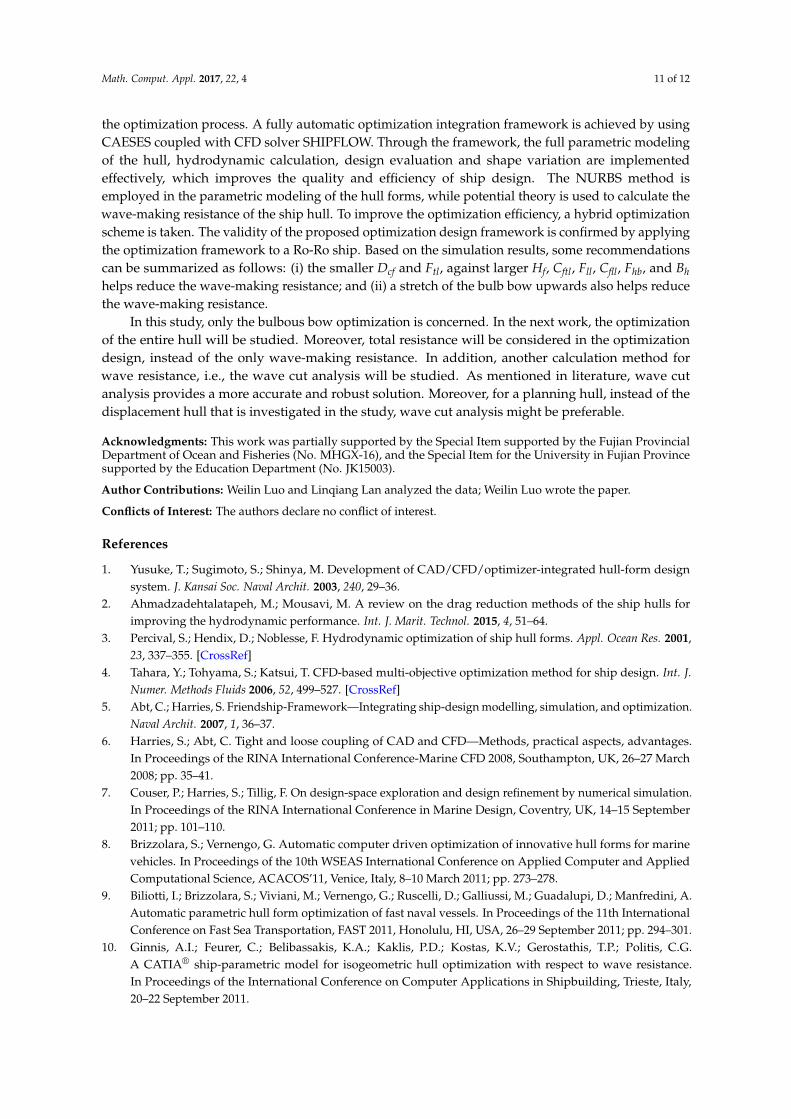
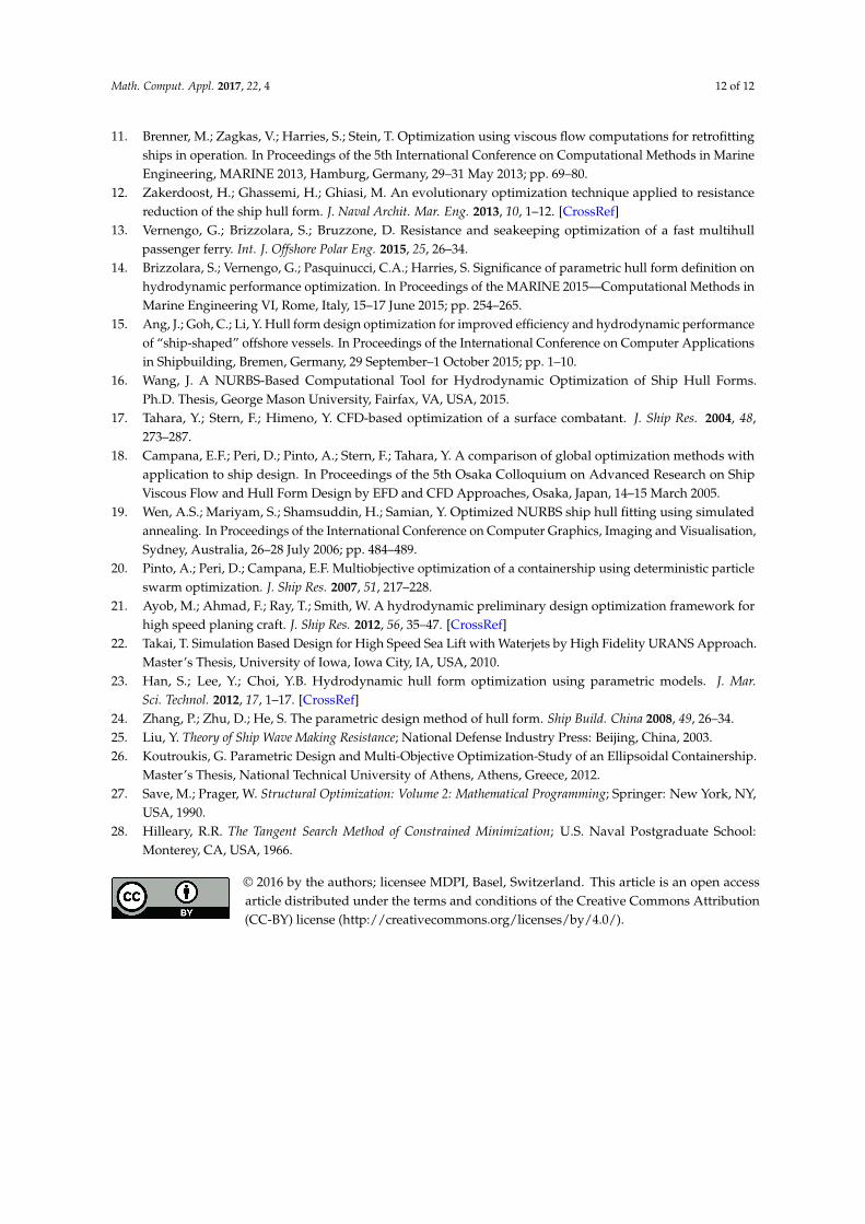
As can be seen from the wave variation, the wave numbers and the wave amplitude decreaseobviously around the bow after the lines of the bulb bow are optimized, which implies a decreaseof wave-making resistance. Figures 9 and 10 present the variation of the lines of the bulb bow.

Math. Comput. Appl. 2017, 22, 4 10 of 12

In Figure 9, the left plot is the original form of the bulb bow, while the right plot is the optimized form.In Figure 10, the yellow lines represent the optimized results while the black lines are with the originalform. From the comparison results, it can be indicated that a stretch of the bulb bow upwards helpsreduce the wave-making resistance.

Math. Comput. Appl. 2017, 22, 4  9 of 12 

longtitudinal section; Fhb, the contour fullness at the half beam of the bulb bow; Bh, half of the maximal 

breadth of the bulb bow. 

Table 4. Optimization results of the objective and constraints. 

Description  Initial Value Optimized Value  Variation 

Nondimensional wave‐making 

resistance, Cw 0.0020368  0.0019488  4.32% (↓) 

Displacement, Δ(t)  22357.695  22382.706  0.112% (↑) Longitudal coordiante of boyance 

center, LCB (m) 0.515798  0.515262  0.104% (↓) 

As  can  be  seen  from  the  optimization  results,  the  wave‐making  resistance  is  reduced  by 

modifying  the  design  variables while  the  constraints  are  satisfied.  The  initial  values  of  design 

variables are one set of the feasible solutions family. The variation of the design variables indicates 

that smaller Dcf and Ftl, against larger Hf, Cftl, Fll, Cfll, Fhb, and Bh help reduce the wave‐making resistance. 

The comparison of the wave contours on free surfaces before and after optimization is presented in 

Figure 7. The comparison of  the  longitudinal wave cuts before and after optimization  is given as 

Figure 8. The right plot in Figure 7 presents the changes of wave contours on the forward part of the 

ship. Similarly, in Figure 8, the right plot highlights the changes of wave cuts on the area around the 

bulbous bow. 

   

Figure 7. Comparison of  the wave contours on  free surfaces before and after optimization; upper 

part,—before optimization; lower part,—after optimization. 

 Figure 8. Comparison of the longitudinal wave cuts before and after optimization (y/L = 0.1). L, ship 

length; units in m/m. Figure 8. Comparison of the longitudinal wave cuts before and after optimization (y/L = 0.1).L, ship length; units in m/m.

Math. Comput. Appl. 2017, 22, 4  10 of 12 

As can be seen from the wave variation, the wave numbers and the wave amplitude decrease 

obviously around the bow after the lines of the bulb bow are optimized, which implies a decrease of 

wave‐making resistance. Figures 9 and 10 present the variation of the lines of the bulb bow. In Figure 

9,  the  left plot  is  the original  form of  the bulb bow, while  the right plot  is  the optimized  form.  In 

Figure 10, the yellow lines represent the optimized results while the black lines are with the original 

form. From the comparison results, it can be indicated that a stretch of the bulb bow upwards helps 

reduce the wave‐making resistance. 

   

Figure  9. Comparison of  the bulbous bows before  and  after optimization:  left,—original;  right,—

optimized. 

 

Figure 10. Comparison of the lines before and after optimization. 

7. Conclusions 

The combination of CFD and CAD improves the quality of ship hull form design. In this paper, 

an  optimization  design  strategy  is  proposed  based  on  SHIPFLOW‐CAESES  framework.  The 

optimization results demonstrate the feasibility of using successfully different software systems in 

the optimization process. A fully automatic optimization integration framework is achieved by using 

CAESES  coupled  with  CFD  solver  SHIPFLOW.  Through  the  framework,  the  full  parametric 

modeling  of  the  hull,  hydrodynamic  calculation,  design  evaluation  and  shape  variation  are 

implemented  effectively, which  improves  the  quality  and  efficiency  of  ship design. The NURBS 

method is employed in the parametric modeling of the hull forms, while potential theory is used to 

calculate  the wave‐making  resistance of  the  ship hull. To  improve  the optimization  efficiency,  a 

hybrid optimization scheme is taken. The validity of the proposed optimization design framework is 

confirmed by applying the optimization framework to a Ro‐Ro ship. Based on the simulation results, 

some recommendations can be summarized as follows: (i) the smaller Dcf and Ftl, against larger Hf, 

Cftl, Fll, Cfll, Fhb, and Bh helps reduce the wave‐making resistance; and (ii) a stretch of the bulb bow 

upwards also helps reduce the wave‐making resistance. 

In this study, only the bulbous bow optimization is concerned. In the next work, the optimization 

of the entire hull will be studied. Moreover, total resistance will be considered in the optimization 

design, instead of the only wave‐making resistance. In addition, another calculation method for wave 

resistance, i.e., the wave cut analysis will be studied. As mentioned in literature, wave cut analysis 

Figure 9. Comparison of the bulbous bows before and after optimization: left,—original;right,—optimized.

Math. Comput. Appl. 2017, 22, 4  10 of 12 

As can be seen from the wave variation, the wave numbers and the wave amplitude decrease 

obviously around the bow after the lines of the bulb bow are optimized, which implies a decrease of 

wave‐making resistance. Figures 9 and 10 present the variation of the lines of the bulb bow. In Figure 

9,  the  left plot  is  the original  form of  the bulb bow, while  the right plot  is  the optimized  form.  In 

Figure 10, the yellow lines represent the optimized results while the black lines are with the original 

form. From the comparison results, it can be indicated that a stretch of the bulb bow upwards helps 

reduce the wave‐making resistance. 

   

Figure  9. Comparison of  the bulbous bows before  and  after optimization:  left,—original;  right,—

optimized. 

 

Figure 10. Comparison of the lines before and after optimization. 

7. Conclusions 

The combination of CFD and CAD improves the quality of ship hull form design. In this paper, 

an  optimization  design  strategy  is  proposed  based  on  SHIPFLOW‐CAESES  framework.  The 

optimization results demonstrate the feasibility of using successfully different software systems in 

the optimization process. A fully automatic optimization integration framework is achieved by using 

CAESES  coupled  with  CFD  solver  SHIPFLOW.  Through  the  framework,  the  full  parametric 

modeling  of  the  hull,  hydrodynamic  calculation,  design  evaluation  and  shape  variation  are 

implemented  effectively, which  improves  the  quality  and  efficiency  of  ship design. The NURBS 

method is employed in the parametric modeling of the hull forms, while potential theory is used to 

calculate  the wave‐making  resistance of  the  ship hull. To  improve  the optimization  efficiency,  a 

hybrid optimization scheme is taken. The validity of the proposed optimization design framework is 

confirmed by applying the optimization framework to a Ro‐Ro ship. Based on the simulation results, 

some recommendations can be summarized as follows: (i) the smaller Dcf and Ftl, against larger Hf, 

Cftl, Fll, Cfll, Fhb, and Bh helps reduce the wave‐making resistance; and (ii) a stretch of the bulb bow 

upwards also helps reduce the wave‐making resistance. 

In this study, only the bulbous bow optimization is concerned. In the next work, the optimization 

of the entire hull will be studied. Moreover, total resistance will be considered in the optimization 

design, instead of the only wave‐making resistance. In addition, another calculation method for wave 

resistance, i.e., the wave cut analysis will be studied. As mentioned in literature, wave cut analysis 

Figure 10. Comparison of the lines before and after optimization.

7. Conclusions

The combination of CFD and CAD improves the quality of ship hull form design. In this paper,an optimization design strategy is proposed based on SHIPFLOW-CAESES framework.The optimization results demonstrate the feasibility of using successfully different software systems in

Math. Comput. Appl. 2017, 22, 4 11 of 12

the optimization process. A fully automatic optimization integration framework is achieved by usingCAESES coupled with CFD solver SHIPFLOW. Through the framework, the full parametric modelingof the hull, hydrodynamic calculation, design evaluation and shape variation are implementedeffectively, which improves the quality and efficiency of ship design. The NURBS method isemployed in the parametric modeling of the hull forms, while potential theory is used to calculate thewave-making resistance of the ship hull. To improve the optimization efficiency, a hybrid optimizationscheme is taken. The validity of the proposed optimization design framework is confirmed by applyingthe optimization framework to a Ro-Ro ship. Based on the simulation results, some recommendationscan be summarized as follows: (i) the smaller Dcf and Ftl, against larger Hf, Cftl, Fll, Cfll, Fhb, and Bhhelps reduce the wave-making resistance; and (ii) a stretch of the bulb bow upwards also helps reducethe wave-making resistance.

In this study, only the bulbous bow optimization is concerned. In the next work, the optimizationof the entire hull will be studied. Moreover, total resistance will be considered in the optimizationdesign, instead of the only wave-making resistance. In addition, another calculation method forwave resistance, i.e., the wave cut analysis will be studied. As mentioned in literature, wave cutanalysis provides a more accurate and robust solution. Moreover, for a planning hull, instead of thedisplacement hull that is investigated in the study, wave cut analysis might be preferable.

Acknowledgments: This work was partially supported by the Special Item supported by the Fujian ProvincialDepartment of Ocean and Fisheries (No. MHGX-16), and the Special Item for the University in Fujian Provincesupported by the Education Department (No. JK15003).

Author Contributions: Weilin Luo and Linqiang Lan analyzed the data; Weilin Luo wrote the paper.

Conflicts of Interest: The authors declare no conflict of interest.

References

1. Yusuke, T.; Sugimoto, S.; Shinya, M. Development of CAD/CFD/optimizer-integrated hull-form designsystem. J. Kansai Soc. Naval Archit. 2003, 240, 29–36.

2. Ahmadzadehtalatapeh, M.; Mousavi, M. A review on the drag reduction methods of the ship hulls forimproving the hydrodynamic performance. Int. J. Marit. Technol. 2015, 4, 51–64.

3. Percival, S.; Hendix, D.; Noblesse, F. Hydrodynamic optimization of ship hull forms. Appl. Ocean Res. 2001,23, 337–355. [CrossRef]

4. Tahara, Y.; Tohyama, S.; Katsui, T. CFD-based multi-objective optimization method for ship design. Int. J.Numer. Methods Fluids 2006, 52, 499–527. [CrossRef]

5. Abt, C.; Harries, S. Friendship-Framework—Integrating ship-design modelling, simulation, and optimization.Naval Archit. 2007, 1, 36–37.

6. Harries, S.; Abt, C. Tight and loose coupling of CAD and CFD—Methods, practical aspects, advantages.In Proceedings of the RINA International Conference-Marine CFD 2008, Southampton, UK, 26–27 March2008; pp. 35–41.

7. Couser, P.; Harries, S.; Tillig, F. On design-space exploration and design refinement by numerical simulation.In Proceedings of the RINA International Conference in Marine Design, Coventry, UK, 14–15 September2011; pp. 101–110.

8. Brizzolara, S.; Vernengo, G. Automatic computer driven optimization of innovative hull forms for marinevehicles. In Proceedings of the 10th WSEAS International Conference on Applied Computer and AppliedComputational Science, ACACOS’11, Venice, Italy, 8–10 March 2011; pp. 273–278.

9. Biliotti, I.; Brizzolara, S.; Viviani, M.; Vernengo, G.; Ruscelli, D.; Galliussi, M.; Guadalupi, D.; Manfredini, A.Automatic parametric hull form optimization of fast naval vessels. In Proceedings of the 11th InternationalConference on Fast Sea Transportation, FAST 2011, Honolulu, HI, USA, 26–29 September 2011; pp. 294–301.

10. Ginnis, A.I.; Feurer, C.; Belibassakis, K.A.; Kaklis, P.D.; Kostas, K.V.; Gerostathis, T.P.; Politis, C.G.A CATIA® ship-parametric model for isogeometric hull optimization with respect to wave resistance.In Proceedings of the International Conference on Computer Applications in Shipbuilding, Trieste, Italy,20–22 September 2011.

Math. Comput. Appl. 2017, 22, 4 12 of 12

11. Brenner, M.; Zagkas, V.; Harries, S.; Stein, T. Optimization using viscous flow computations for retrofittingships in operation. In Proceedings of the 5th International Conference on Computational Methods in MarineEngineering, MARINE 2013, Hamburg, Germany, 29–31 May 2013; pp. 69–80.

12. Zakerdoost, H.; Ghassemi, H.; Ghiasi, M. An evolutionary optimization technique applied to resistancereduction of the ship hull form. J. Naval Archit. Mar. Eng. 2013, 10, 1–12. [CrossRef]

13. Vernengo, G.; Brizzolara, S.; Bruzzone, D. Resistance and seakeeping optimization of a fast multihullpassenger ferry. Int. J. Offshore Polar Eng. 2015, 25, 26–34.

14. Brizzolara, S.; Vernengo, G.; Pasquinucci, C.A.; Harries, S. Significance of parametric hull form definition onhydrodynamic performance optimization. In Proceedings of the MARINE 2015—Computational Methods inMarine Engineering VI, Rome, Italy, 15–17 June 2015; pp. 254–265.

15. Ang, J.; Goh, C.; Li, Y. Hull form design optimization for improved efficiency and hydrodynamic performanceof “ship-shaped” offshore vessels. In Proceedings of the International Conference on Computer Applicationsin Shipbuilding, Bremen, Germany, 29 September–1 October 2015; pp. 1–10.

16. Wang, J. A NURBS-Based Computational Tool for Hydrodynamic Optimization of Ship Hull Forms.Ph.D. Thesis, George Mason University, Fairfax, VA, USA, 2015.

17. Tahara, Y.; Stern, F.; Himeno, Y. CFD-based optimization of a surface combatant. J. Ship Res. 2004, 48,273–287.

18. Campana, E.F.; Peri, D.; Pinto, A.; Stern, F.; Tahara, Y. A comparison of global optimization methods withapplication to ship design. In Proceedings of the 5th Osaka Colloquium on Advanced Research on ShipViscous Flow and Hull Form Design by EFD and CFD Approaches, Osaka, Japan, 14–15 March 2005.

19. Wen, A.S.; Mariyam, S.; Shamsuddin, H.; Samian, Y. Optimized NURBS ship hull fitting using simulatedannealing. In Proceedings of the International Conference on Computer Graphics, Imaging and Visualisation,Sydney, Australia, 26–28 July 2006; pp. 484–489.

20. Pinto, A.; Peri, D.; Campana, E.F. Multiobjective optimization of a containership using deterministic particleswarm optimization. J. Ship Res. 2007, 51, 217–228.

21. Ayob, M.; Ahmad, F.; Ray, T.; Smith, W. A hydrodynamic preliminary design optimization framework forhigh speed planing craft. J. Ship Res. 2012, 56, 35–47. [CrossRef]

22. Takai, T. Simulation Based Design for High Speed Sea Lift with Waterjets by High Fidelity URANS Approach.Master’s Thesis, University of Iowa, Iowa City, IA, USA, 2010.

23. Han, S.; Lee, Y.; Choi, Y.B. Hydrodynamic hull form optimization using parametric models. J. Mar.Sci. Technol. 2012, 17, 1–17. [CrossRef]

24. Zhang, P.; Zhu, D.; He, S. The parametric design method of hull form. Ship Build. China 2008, 49, 26–34.25. Liu, Y. Theory of Ship Wave Making Resistance; National Defense Industry Press: Beijing, China, 2003.26. Koutroukis, G. Parametric Design and Multi-Objective Optimization-Study of an Ellipsoidal Containership.

Master’s Thesis, National Technical University of Athens, Athens, Greece, 2012.27. Save, M.; Prager, W. Structural Optimization: Volume 2: Mathematical Programming; Springer: New York, NY,

USA, 1990.28. Hilleary, R.R. The Tangent Search Method of Constrained Minimization; U.S. Naval Postgraduate School:

Monterey, CA, USA, 1966.

© 2016 by the authors; licensee MDPI, Basel, Switzerland. This article is an open accessarticle distributed under the terms and conditions of the Creative Commons Attribution(CC-BY) license (http://creativecommons.org/licenses/by/4.0/).