Blade bulbous-bow concept application research …...Blade bulbous-bow concept application research...
82
Blade bulbous-bow concept application research using commercial CFD software Mukhitdin Kakenov Master Thesis presented in partial fulfillment of the requirements for the double degree: “Advanced Master in Naval Architecture” conferred by University of Liege "Master of Sciences in Applied Mechanics, specialization in Hydrodynamics, Energetics and Propulsion” conferred by Ecole Centrale de Nantes developed at University of Genoa, Genoa in the framework of the “EMSHIP” Erasmus Mundus Master Course in “Integrated Advanced Ship Design” EMJMD 159652 – Grant Agreement 2015-1687 Supervisor: Prof.Dario Boote, University of Genoa, Genoa Reviewer: Genoa, February 2018
Transcript of Blade bulbous-bow concept application research …...Blade bulbous-bow concept application research...
Blade bulbous-bow concept application research using commercial CFD software
Mukhitdin Kakenov
Master Thesis
presented in partial fulfillment of the requirements for the double degree:
“Advanced Master in Naval Architecture” conferred by University of Liege "Master of Sciences in Applied Mechanics, specialization in Hydrodynamics,
Energetics and Propulsion” conferred by Ecole Centrale de Nantes developed at University of Genoa, Genoa
in the framework of the
“EMSHIP” Erasmus Mundus Master Course
in “Integrated Advanced Ship Design”
EMJMD 159652 – Grant Agreement 2015-1687
Supervisor: Prof.Dario Boote, University of Genoa, Genoa
Reviewer:
Genoa, February 2018

2
3

4

5
6
Contents
SUMMARY
1. INTRODUCTION ................................................................................................................ 8
2. OVERVIEW OF EXISTING VESSELS USING BLADE BULBOUS BOW ................................... 8
2.1. Dominator Ilumen 28M ............................................................................................. 9
2.2. Benetti F-125 ........................................................................................................... 13
3. PROBLEM TO SOLVE ....................................................................................................... 15
4. MODELLING THE PHYSICS. THEORY PART. ..................................................................... 17
5. WAY TO SOLVE THE PROBLEM ....................................................................................... 21
5.1. Comparison of popular methods ............................................................................ 24
5.2. Chosen method - CFD .............................................................................................. 25
6. MESH CONVERGENCE STUDY ........................................................................................ 26
7. TEST LAUNCHES ............................................................................................................. 32
7.1. Initial bow aimed yacht ........................................................................................... 32
7.2. Blade bow, 1st variant .............................................................................................. 47
7.3. Blade bow, 2nd variant ............................................................................................. 68
CONCLUSION ...................................................................................................................... 81
REFERENCES ....................................................................................................................... 82

7
8
1. INTRODUCTION
From one port to another one, much faster as possible. Much cheaper as possible. Much
more comfortable.
Bulbous bow’s purposes are to fight against head wave impact and decrease drag from
wave generating resistance. These two actions cover such important sections as financial
costs (fuel consumption, hull maintenance cost), transportation time (seakeeping, ship’s
velocity), comfort for passengers and crew (vibration, wave shock impact).
Application of bulbous bow helps to significantly reduce all above listed costs, journey
time and improve people’s health condition onboard. Electronic equipment undergoes
less shock and has less risk to be damaged due to wave impact on fore-part. Hull
vibration levels may also be reduced by high values and frequencies.
But still, there is no limit to try to improve bulbous bow’s performance further.
In this thesis the author will describe and provide the results from research made to find
out about applicability of new concept of bulbous bow – blade bulbous bow – on a
middle-size semi-displacement cruise yachts.
The new bow application already had obtained positive reviews in naval/maritime
theme magazines. Here below some articles will be provided as side overview of existing
vessels aiming such a bow.
2. OVERVIEW OF EXISTING VESSELS USING BLADE BULBOUS BOW
There are at least two yachts the thesis author would like to mention: first one is Ilumen
28M from Dominator shipyard and the second is Benetti’s F-125 (see pictures on figures
2.1-2.7 for the Ilumen 28M and figures 2.8-2.10 for F-125). The sources the photos are
taken from are [1] and [2] for the Ilumen 28M and [3] for the F-125.
9
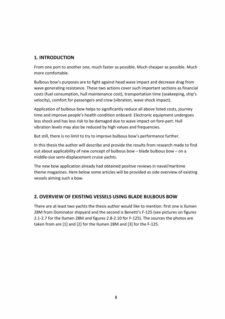
2.1. Dominator Ilumen 28M
Fig.2.1.
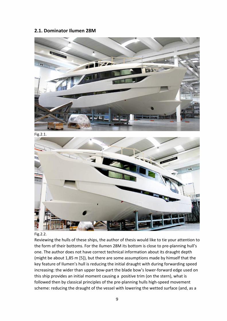
Fig.2.2.
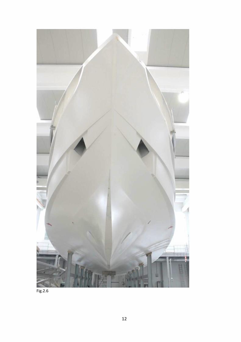
Reviewing the hulls of these ships, the author of thesis would like to tie your attention to
the form of their bottoms. For the Ilumen 28M its bottom is close to pre-planning hull’s
one. The author does not have correct technical information about its draught depth
(might be about 1,85 m [5]), but there are some assumptions made by himself that the
key feature of Ilumen’s hull is reducing the initial draught with during forwarding speed
increasing: the wider than upper bow-part the blade bow’s lower-forward edge used on
this ship provides an initial moment causing a positive trim (on the stern), what is
followed then by classical principles of the pre-planning hulls high-speed movement
scheme: reducing the draught of the vessel with lowering the wetted surface (and, as a
10
result, the frictional drag). This vessel may develop its velocity from 23 knots up to 29
knots, the length on the waterline of the ship is 23.50 meters at half load [5]. The Froude
number is about 1.515 – that should be beyond of the range of the usual pre-planning
regime Froude number range [4], very good fact for the assumptions made. The ship
page on the web-site of the Derani Yachts Co. Ltd. (https://www.derani-
yachts.com/yachts/dominator-ilumen-28-metre/#) states that the ship able to have the
maximal speed for 29 knots and 23 knots for cruising. Relating to the information
collected the author would accept to consider the working speed as about 23 knots. And
even in this case the Froude number still is calculated not lower than 1.4, what keeps
the assumption of the pre-planning regime scheme for this yacht. On the maximal speed
the ship may switch to planning regime, as the Froude number estimates as 1.91.
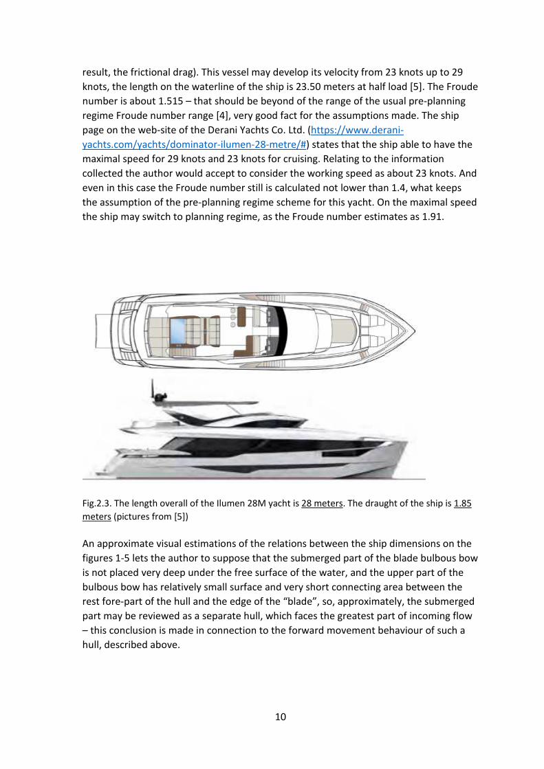
Fig.2.3. The length overall of the Ilumen 28M yacht is 28 meters. The draught of the ship is 1.85
meters (pictures from [5])
An approximate visual estimations of the relations between the ship dimensions on the
figures 1-5 lets the author to suppose that the submerged part of the blade bulbous bow
is not placed very deep under the free surface of the water, and the upper part of the
bulbous bow has relatively small surface and very short connecting area between the
rest fore-part of the hull and the edge of the “blade”, so, approximately, the submerged
part may be reviewed as a separate hull, which faces the greatest part of incoming flow
– this conclusion is made in connection to the forward movement behaviour of such a
hull, described above.
11
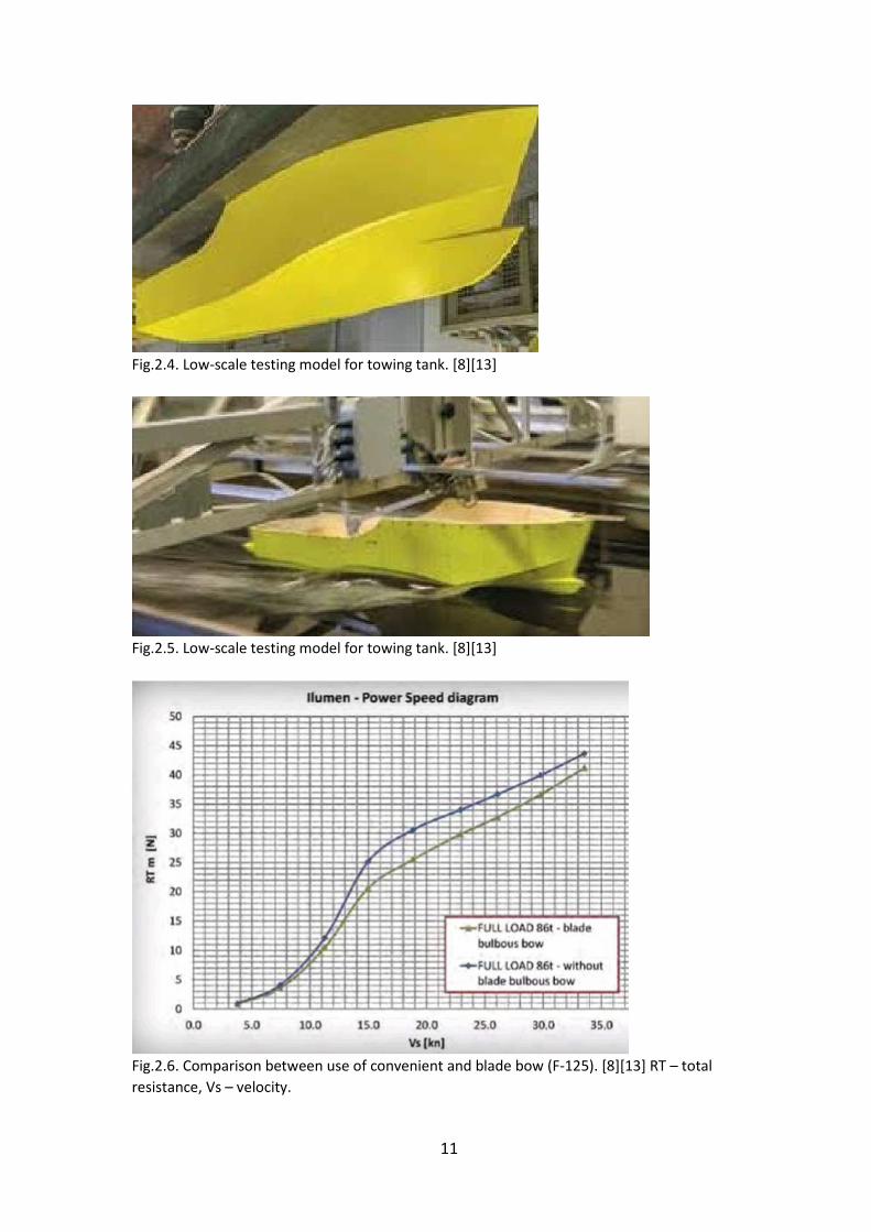
Fig.2.4. Low-scale testing model for towing tank. [8][13]
Fig.2.5. Low-scale testing model for towing tank. [8][13]
Fig.2.6. Comparison between use of convenient and blade bow (F-125). [8][13] RT – total
resistance, Vs – velocity.
12
Fig.2.6
13
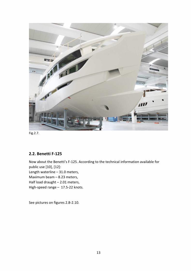
Fig.2.7.
2.2. Benetti F-125
Now about the Benetti’s F-125. According to the technical information available for
public use [10], [12]:
Length waterline – 31.0 meters,
Maximum beam – 8.23 meters,
Half load draught – 2.01 meters,
High-speed range – 17.5-22 knots.
See pictures on figures 2.8-2.10.
14
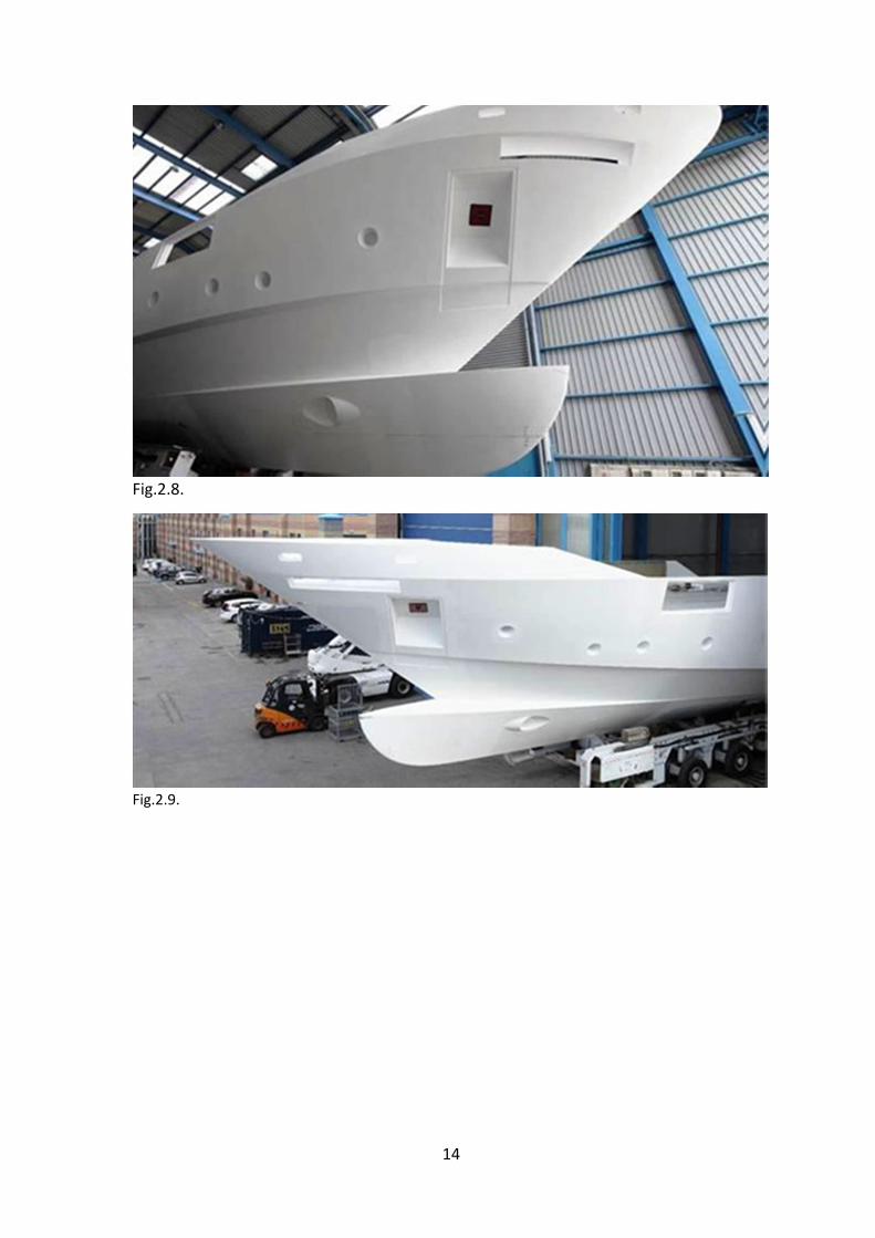
Fig.2.8.
Fig.2.9.
15
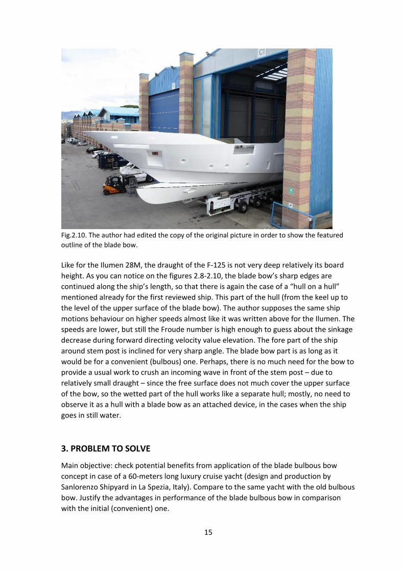
Fig.2.10. The author had edited the copy of the original picture in order to show the featured
outline of the blade bow.
Like for the Ilumen 28M, the draught of the F-125 is not very deep relatively its board
height. As you can notice on the figures 2.8-2.10, the blade bow’s sharp edges are
continued along the ship’s length, so that there is again the case of a “hull on a hull”
mentioned already for the first reviewed ship. This part of the hull (from the keel up to
the level of the upper surface of the blade bow). The author supposes the same ship
motions behaviour on higher speeds almost like it was written above for the Ilumen. The
speeds are lower, but still the Froude number is high enough to guess about the sinkage
decrease during forward directing velocity value elevation. The fore part of the ship
around stem post is inclined for very sharp angle. The blade bow part is as long as it
would be for a convenient (bulbous) one. Perhaps, there is no much need for the bow to
provide a usual work to crush an incoming wave in front of the stem post – due to
relatively small draught – since the free surface does not much cover the upper surface
of the bow, so the wetted part of the hull works like a separate hull; mostly, no need to
observe it as a hull with a blade bow as an attached device, in the cases when the ship
goes in still water.
3. PROBLEM TO SOLVE
Main objective: check potential benefits from application of the blade bulbous bow
concept in case of a 60-meters long luxury cruise yacht (design and production by
Sanlorenzo Shipyard in La Spezia, Italy). Compare to the same yacht with the old bulbous
bow. Justify the advantages in performance of the blade bulbous bow in comparison
with the initial (convenient) one.
16
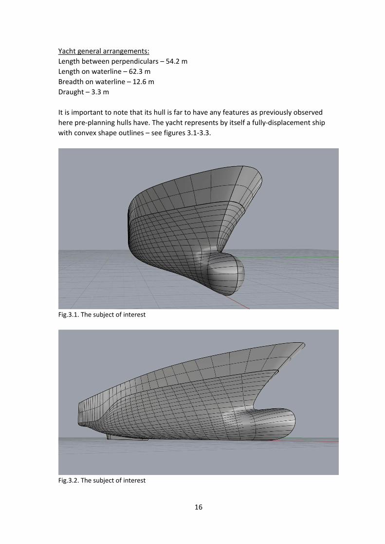
Yacht general arrangements:
Length between perpendiculars – 54.2 m
Length on waterline – 62.3 m
Breadth on waterline – 12.6 m
Draught – 3.3 m
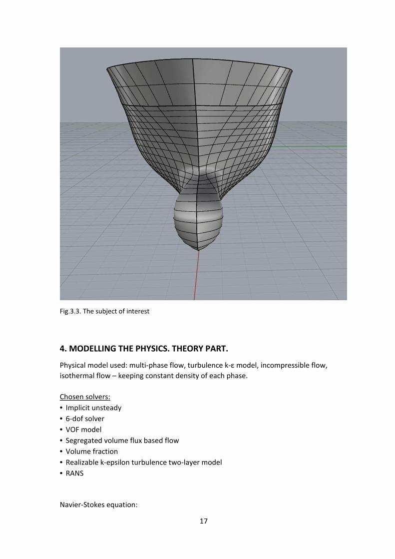
It is important to note that its hull is far to have any features as previously observed
here pre-planning hulls have. The yacht represents by itself a fully-displacement ship
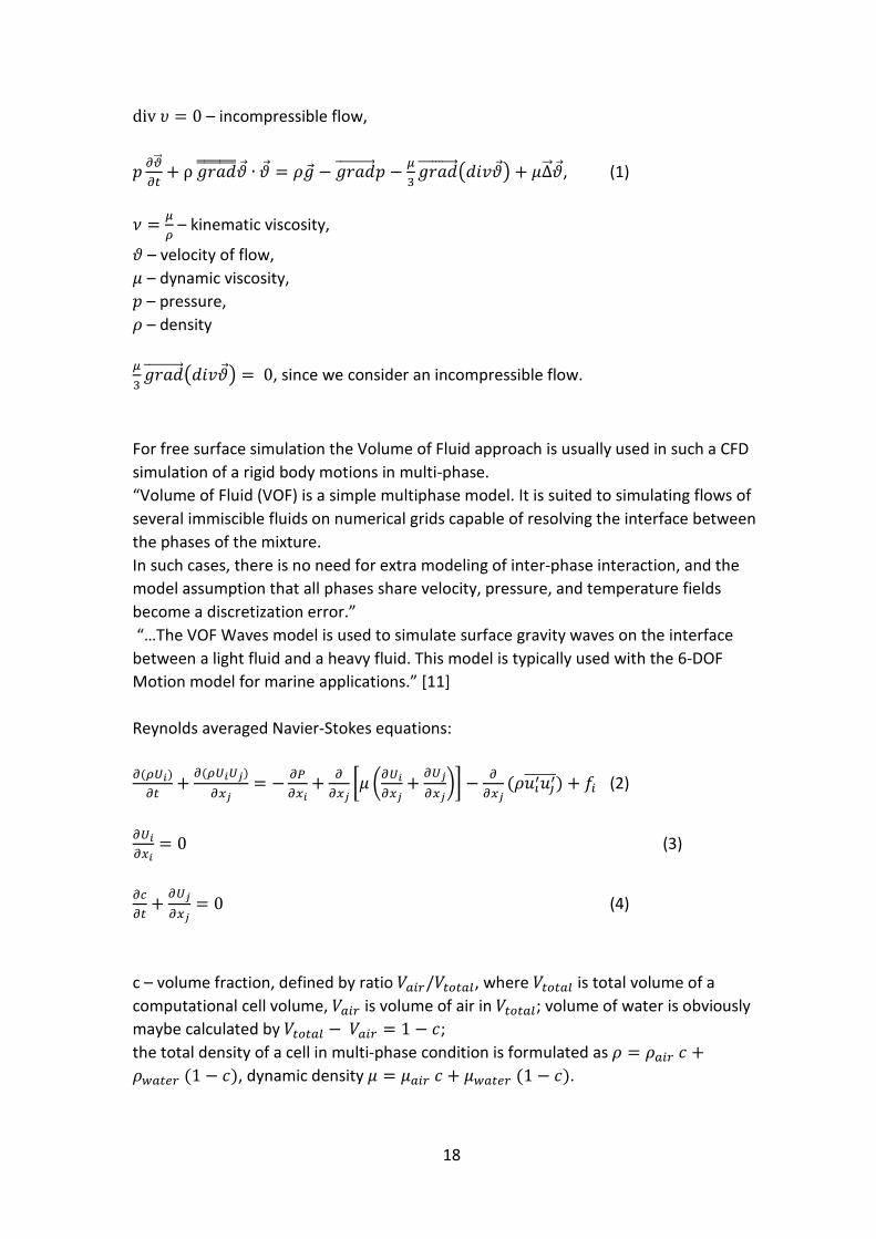
with convex shape outlines – see figures 3.1-3.3.
Fig.3.1. The subject of interest
Fig.3.2. The subject of interest
17
Fig.3.3. The subject of interest
4. MODELLING THE PHYSICS. THEORY PART.
Physical model used: multi-phase flow, turbulence k-ε model, incompressible flow,
isothermal flow – keeping constant density of each phase.
Chosen solvers:
• Implicit unsteady
• 6-dof solver
• VOF model
• Segregated volume flux based flow
• Volume fraction
• Realizable k-epsilon turbulence two-layer model
• RANS
Navier-Stokes equation:
18
div � = 0 – incompressible flow,
� ��� + ρ ������������� ∙ �� = ��� − ���������������� − �
� ���������������������� + �∆�����, (1)
! = �" – kinematic viscosity,
� – velocity of flow,
� – dynamic viscosity,
� – pressure,
� – density
�� ���������������������� = 0, since we consider an incompressible flow.
For free surface simulation the Volume of Fluid approach is usually used in such a CFD
simulation of a rigid body motions in multi-phase.
“Volume of Fluid (VOF) is a simple multiphase model. It is suited to simulating flows of
several immiscible fluids on numerical grids capable of resolving the interface between
the phases of the mixture.
In such cases, there is no need for extra modeling of inter-phase interaction, and the
model assumption that all phases share velocity, pressure, and temperature fields
become a discretization error.”
“…The VOF Waves model is used to simulate surface gravity waves on the interface
between a light fluid and a heavy fluid. This model is typically used with the 6-DOF
Motion model for marine applications.” [11]
Reynolds averaged Navier-Stokes equations:
("$%) + ("$%$')
('= − )
(%+
('*� +$%
('+ $'
(',- −
('(�./0.10222222) + 34 (2)
$%(%
= 0 (3)
5 + $'
('= 0 (4)
с – volume fraction, defined by ratio 6748/6 : 7;, where 6 : 7; is total volume of a
computational cell volume, 6748 is volume of air in 6 : 7;; volume of water is obviously
maybe calculated by 6 : 7; − 6748 = 1 − =;
the total density of a cell in multi-phase condition is formulated as � = �748 = +�>7 ?8 (1 − =), dynamic density � = �748 = + �>7 ?8 (1 − =).
19
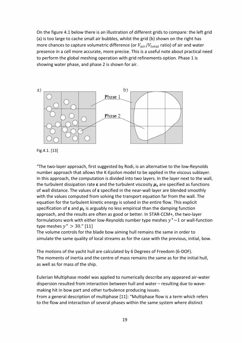
On the figure 4.1 below there is an illustration of different grids to compare: the left grid
(a) is too large to cache small air bubbles, whilst the grid (b) shown on the right has
more chances to capture volumetric difference (or 6748/6 : 7; ratio) of air and water
presence in a cell more accurate, more precise. This is a useful note about practical need
to perform the global meshing operation with grid refinements option. Phase 1 is
showing water phase, and phase 2 is shown for air.
Fig.4.1. [13]
“The two-layer approach, first suggested by Rodi, is an alternative to the low-Reynolds
number approach that allows the K-Epsilon model to be applied in the viscous sublayer.
In this approach, the computation is divided into two layers. In the layer next to the wall,
the turbulent dissipation rate ε and the turbulent viscosity @A are specified as functions
of wall distance. The values of ε specified in the near-wall layer are blended smoothly
with the values computed from solving the transport equation far from the wall. The
equation for the turbulent kinetic energy is solved in the entire flow. This explicit
specification of ε and @A is arguably no less empirical than the damping function
approach, and the results are often as good or better. In STAR-CCM+, the two-layer
formulations work with either low-Reynolds number type meshes BC~1 or wall-function
type meshes BC E 30.” [11] The volume controls for the blade bow aiming hull remains the same in order to
simulate the same quality of local streams as for the case with the previous, initial, bow.
The motions of the yacht hull are calculated by 6 Degrees of Freedom (6-DOF).
The moments of inertia and the centre of mass remains the same as for the initial hull,
as well as for mass of the ship.
Eulerian Multiphase model was applied to numerically describe any appeared air-water
dispersion resulted from interaction between hull and water – resulting due to wave-
making hit in bow part and other turbulence producing issues.
From a general description of multiphase [11]: “Multiphase flow is a term which refers
to the flow and interaction of several phases within the same system where distinct
20
interfaces exist between the phases. The term ‘phase’ usually refers to the
thermodynamic state of the matter: solid, liquid, or gas.
In modelling terms, a phase is defined in broader terms, and can be defined as a
quantity of matter within a system that has its own physical properties to distinguish it
from other phases within the system. For example:
Liquids of different density
Bubbles of different size
Particles of different shape
Multiphase flows are different from multi-component flows. In multi-component flows,
the different species are mixed at the molecular level. These species have the same
convection velocity. In multiphase flows, the different phases are mixed at the
macroscopic scale. These phases have different convection velocity. Many flows are
multiphase multi-component flows.
Multiphase flows can be classified into two categories:
Dispersed flows, such as bubbly, droplet, and particle flows
Stratified flows, such as free surface flows, or annular film flow in pipes.
A phase is considered dispersed if it occupies disconnected regions of space—otherwise
it is continuous.”
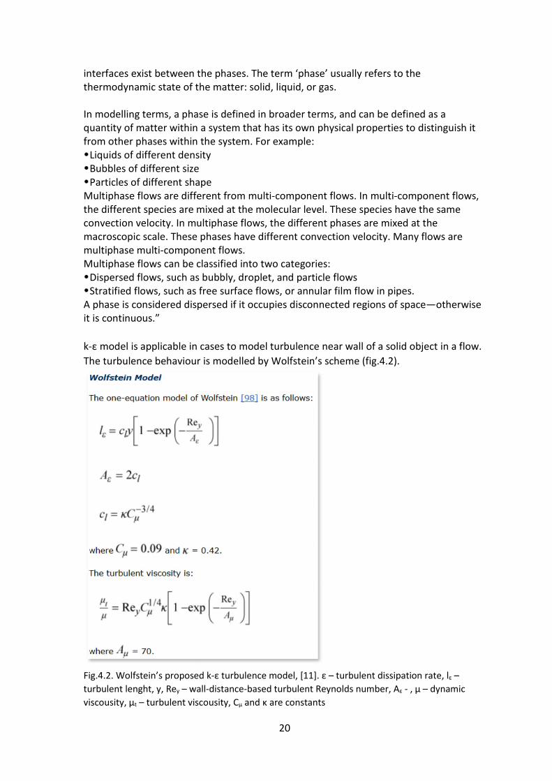
k-ε model is applicable in cases to model turbulence near wall of a solid object in a flow.
The turbulence behaviour is modelled by Wolfstein’s scheme (fig.4.2).
Fig.4.2. Wolfstein’s proposed k-ε turbulence model, [11]. ε – turbulent dissipation rate, lε –
turbulent lenght, y, Rey – wall-distance-based turbulent Reynolds number, Aε - , μ – dynamic
viscousity, μt – turbulent viscousity, Cμ and κ are constants
21
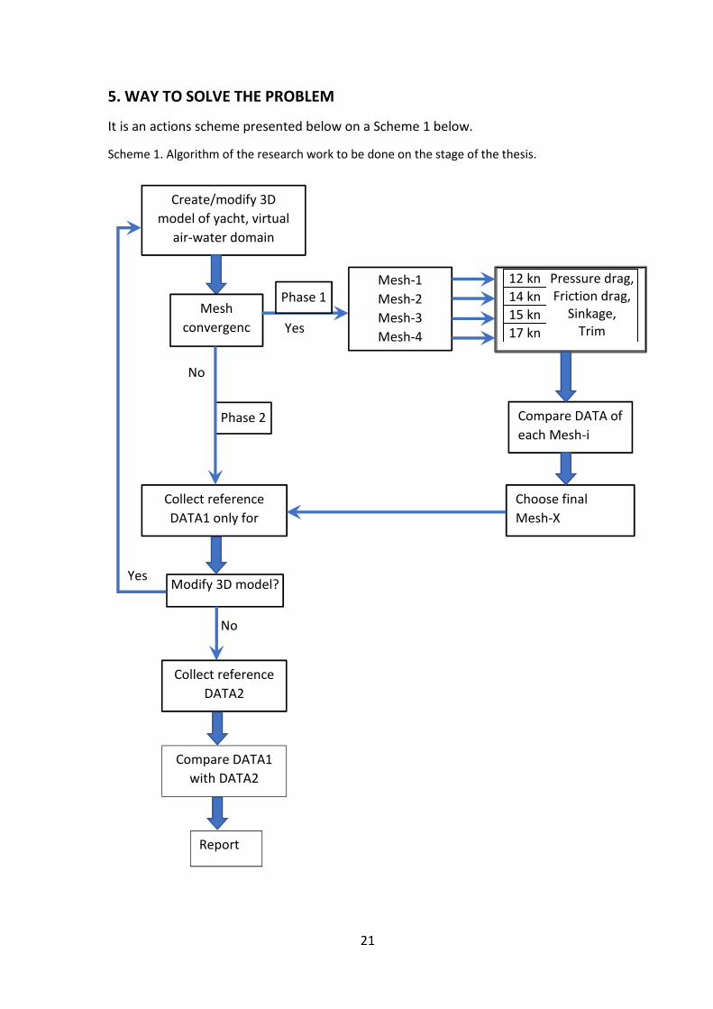
5. WAY TO SOLVE THE PROBLEM
It is an actions scheme presented below on a Scheme 1 below.
Scheme 1. Algorithm of the research work to be done on the stage of the thesis.
Report
Create/modify 3D
model of yacht, virtual
air-water domain
Modify 3D model?
Mesh
convergenc
e?
12 kn Pressure drag,
Friction drag,
Sinkage,
Trim
14 kn
15 kn
17 kn
Phase 2
Phase 1
No
Yes
Mesh-1
Mesh-2
Mesh-3
Mesh-4
Compare DATA of
each Mesh-i
setting
Choose final
Mesh-X
Collect reference
DATA1 only for
Phase 1
Yes
No
Collect reference
DATA2
Compare DATA1
with DATA2

22
I. Collect reference data of motions, forces and moments of the yacht hull with the
old bow for different velocities.
II. Test new bow in the same conditions.
III. Compare both data collected, make conclusion.
Notes about the new bow construction: the shape of blade bow was sketched and made
by those blade bulbous bows presented on magazines photos, no special drafts were
used; the new bow has to be limited by the main dimensions (length, breadth, height) of
the old one. Main shape features of this kind of bow were accepted are: flat horizontal
plane on top of the bow, transversal profile flows from U-shaped into V-shaped
sharpening on the forward continuing keel line. However, transverse section may also be
shaped as an inequilateral rhomb. The next important feature should be mentioned, due
to difficulties of connection the triangle shape of the blade bulbous bow with the yacht
hull (and any other one, as visual appearance shows so) the hull part between the blade
bow and the hull became wider than in case with the old convenient bow. The tests will
show how much higher will be the pressure (and friction) drag of the new model of
yacht. See figures 5.1-5.5 (taken from the articles [8-9]).
Fig.5.1. “Dominator Ilumen 28M”
23
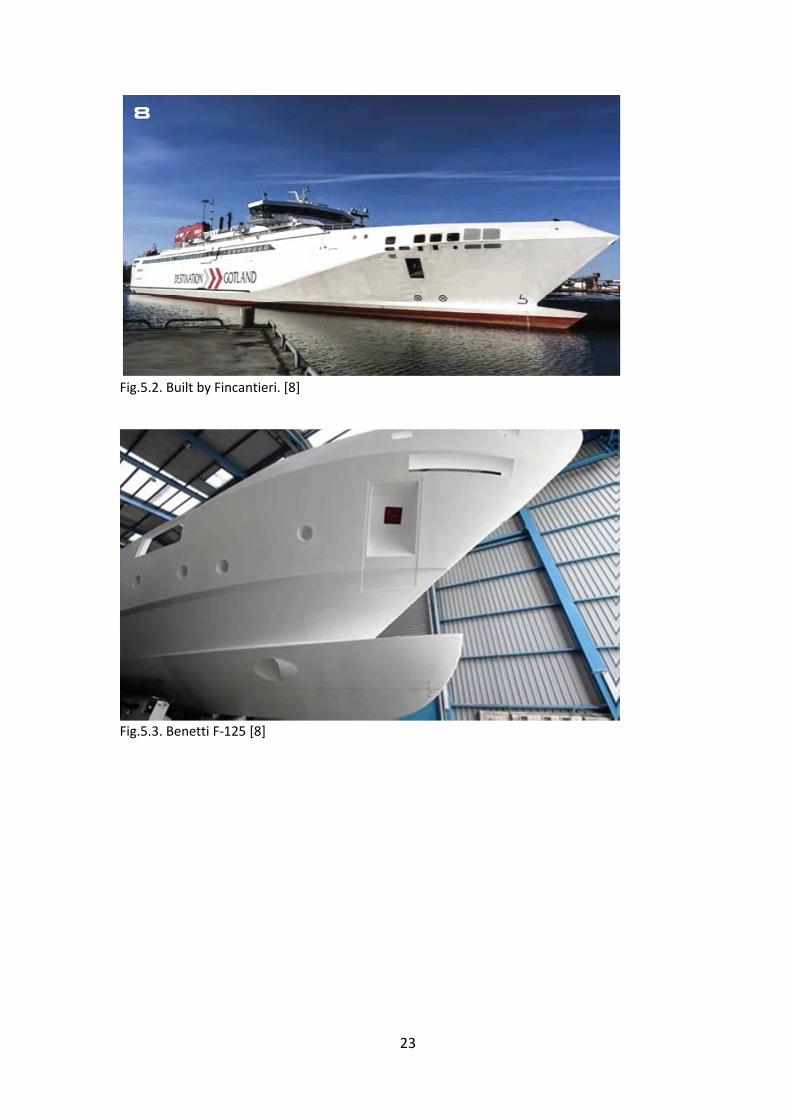
Fig.5.2. Built by Fincantieri. [8]
Fig.5.3. Benetti F-125 [8]
24
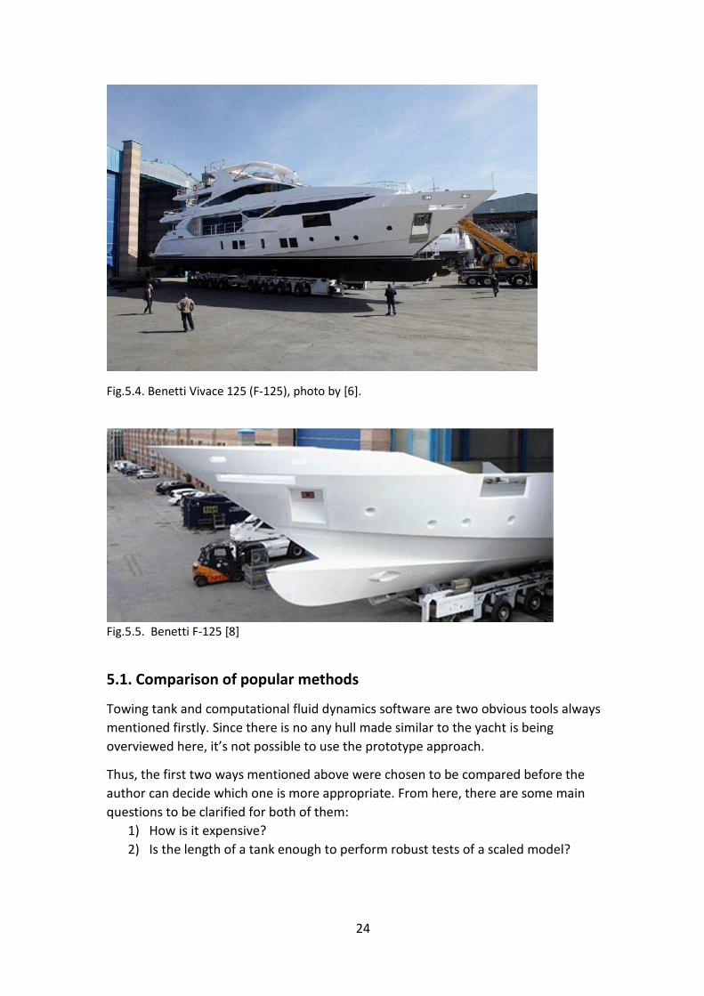
Fig.5.4. Benetti Vivace 125 (F-125), photo by [6].
Fig.5.5. Benetti F-125 [8]
5.1. Comparison of popular methods
Towing tank and computational fluid dynamics software are two obvious tools always
mentioned firstly. Since there is no any hull made similar to the yacht is being
overviewed here, it’s not possible to use the prototype approach.
Thus, the first two ways mentioned above were chosen to be compared before the
author can decide which one is more appropriate. From here, there are some main
questions to be clarified for both of them:
1) How is it expensive?
2) Is the length of a tank enough to perform robust tests of a scaled model?
25
3) What is the biggest scale may be used in chosen tank until the standard
conditions of towing tank tests (to avoid the walls and scale effect) will be
overstepped?
4) How long will it take to provide such a test in the chosen tank with the chosen
model scale? Including standard preparations and test process - overall.
5) What percentage of errors may occur during processing experimental and
numerical tests and which approach usually shows less measurements deviations
over the full-scale tests? By other words, which tool shows better convergence
with the same measurements for real ship?
Towing tank tests requires much less financial expenses than numerical one.
But in case of the model size may be used, the numerical approach for sure has an
advantage here, since there is almost no any size limit for an object which needs to be
analysed, whilst enough CPU power and RAM were provided for it.
5.2. Chosen method - CFD
The commercial CFD software STAR-CCM+ had been chosen to simulate yacht
movements on different speeds and then obtain the measurements of forces and
moments acting on the ship, recording sinkage and trim behaviour.
The standard way of simulation setting was used: deep and wide virtual “towing tank” to
avoid wall effects and have more available space to apply fine enough mesh in air-water
domain around the yacht hull for modelling fluid behaviour as more realistic as possible,
in order to reduce the calculation error.
All technical requirements of experimental equipment needed was defined as for a
computer with 20 cores with CPU power minimum 1.7 GHz each, at least 12 GB RAM
memory and space on hard drive about 2 GB for each simulation file (total number of
simulations had been done during research work was 22 sets, including mesh
convergence study, reference data collection and the same data refreshing by launching
the yacht with the new bow mounted on virtual model).
3D model of the initial yacht hull and the modified one were made by using the
commercial CAD software Rhinoceros. Meshing operations were performed by STAR-
CCM+’s inner meshing tool.
The model was tested in the STAR-CCM+ as full-scale, avoiding possible mistakes from
rescaling the results obtained in case of using smaller hull.
26
6. MESH CONVERGENCE STUDY
Comparison was made by shear and pressure drag of the yacht hull depending on the
number of cells used for a solution. Each drag diagram curve had been resulted by
points from each speed given by 14, 15, 17 knots.
Since number of cells directly dependent from a base size chosen in STAR-CCM+, author
also notes different base size values in the same comparing table as alternative
reference value instead of number of cells. This had been done to show the relation
between all given dimensions (virtual air-water domain, ship’s general arrangements,
volumetric refinements done) – in order to study a practical approach to current
commercial software when dealing with the same subject of interest as a middle-speed
vessel in still water conditions. The Base size is a value which is taken as reference one,
all main volumetric and surface mesh refinements are taken by percentage from this
value. Whilst base size is being varied the percentage of each mesh control remains the
same. In the program this value is set in reference to specific area covered around the
ship, and defined by volumetric refinements.
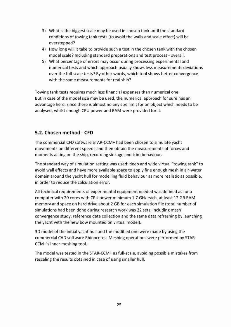
Table 1
Number of
cells = 891486;
Base size = 10
m
Velocity,
kn
Shear drag, kN Pressure drag, kN Sinkage, m Trim, deg
14 19.76657115 26.63347473 -0.176262845 0.494623313 15 22.74049515 31.94867126 -0.219005168 0.528570385 17 29.21494457 55.07470809 -0.291786416 0.6319012
Table 2
Number of
cells =
1673806;
Base size = 7.5
m
Velocity,
kn
Shear drag, kN Pressure drag, kN Sinkage, m Trim, deg
14 19.88839339 25.50340452 -0.175948402 0.487821608 15 22.71141888 30.60855957 -0.216470852 0.519347939 17 29.3228924 54.75375905 -0.293865647 0.602759934
Table 3
Number of
cells =
2989818;
Base size = 6 m
Velocity,
kn
Shear drag, kN Pressure drag, kN Sinkage, m Trim, deg
14 19.88163236 24.44349585 -0.173079991 0.49611262 15 22.81391047 30.11767118 -0.214673105 0.529019871 17 29.40883949 54.13670687 -0.292880558 0.598633927
According the results had been obtained, the most suitable number of cells will be for
1.7 million (mln) cells. Comparing modelling for 1.7 mln cells with 3 mln cells modelling,
the wall time to calculate 1.7 mln cells was approximately for 15 hours less.

27
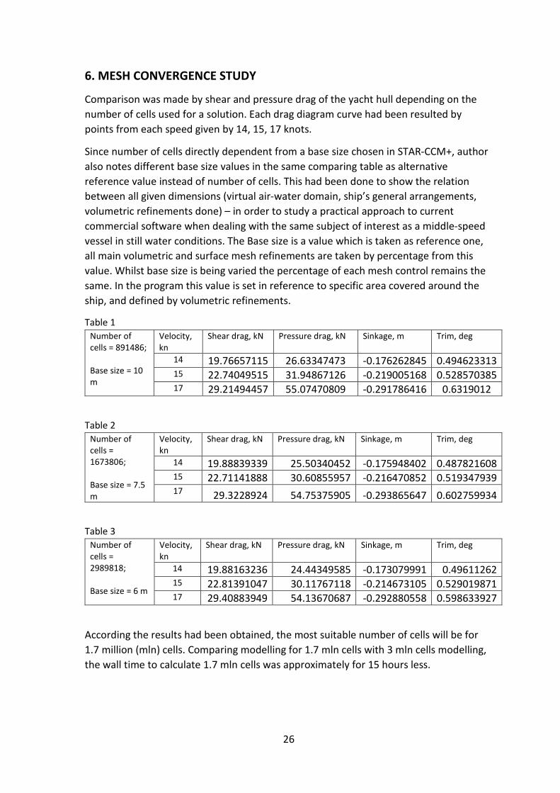
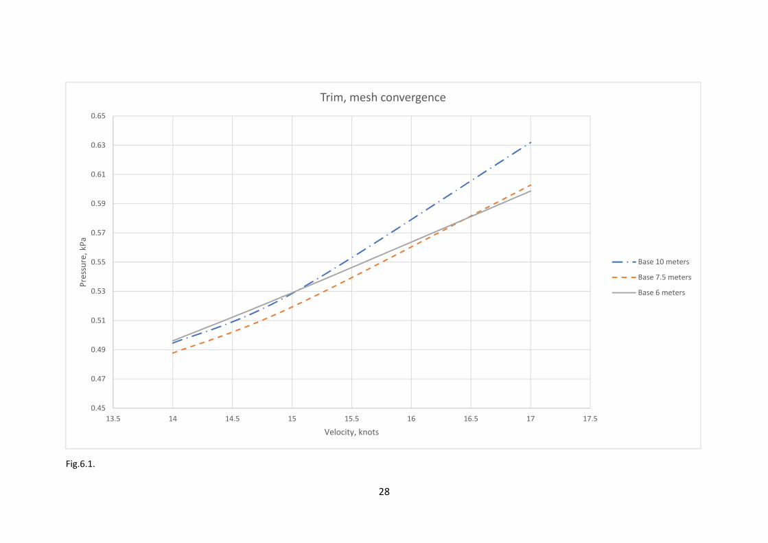
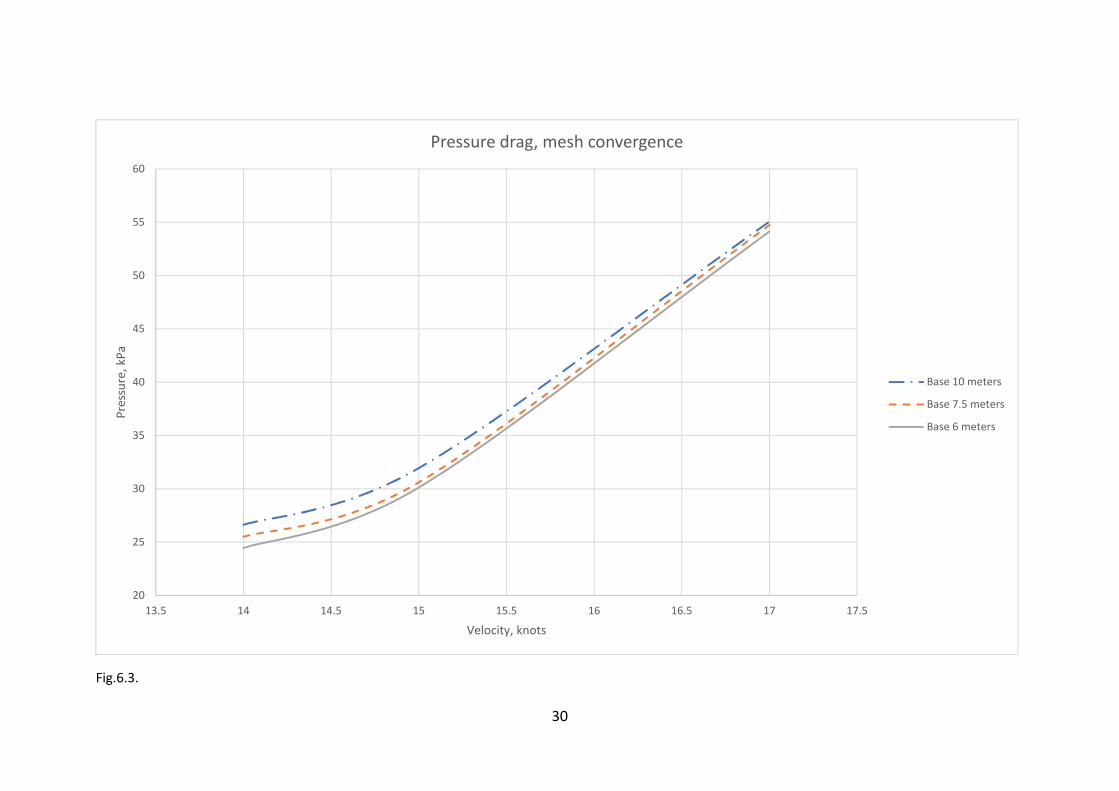
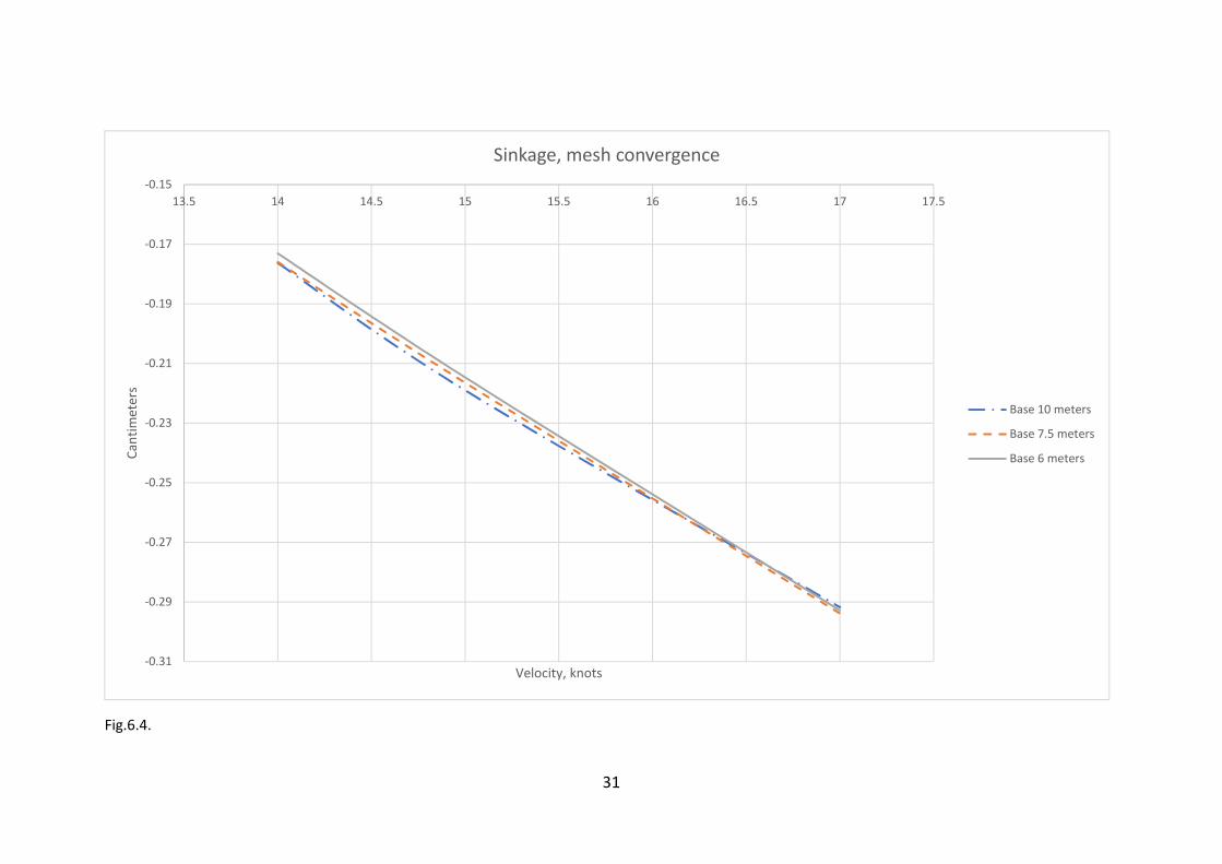
Take a look on the figures 6.1-6.4. Comparison between frictional resistance, pressure
drag, trim an sinkage are presented on those pictures, in order to visually evaluate which
mesh grid fits another with the best match.
28
Fig.6.1.
0.45
0.47
0.49
0.51
0.53
0.55
0.57
0.59
0.61
0.63
0.65
13.5 14 14.5 15 15.5 16 16.5 17 17.5
Pre
ssu
re,
kP
a
Velocity, knots
Trim, mesh convergence
Base 10 meters
Base 7.5 meters
Base 6 meters
29
Fig.6.2.
19
21
23
25
27
29
31
13.5 14 14.5 15 15.5 16 16.5 17 17.5
Fo
rce
, k
N
Velocity, knots
Shear drag, mesh convergence
Base 10 meters
Base 7.5 meters
Base 6 meters
30
Fig.6.3.
20
25
30
35
40
45
50
55
60
13.5 14 14.5 15 15.5 16 16.5 17 17.5
Pre
ssu
re,
kP
a
Velocity, knots
Pressure drag, mesh convergence
Base 10 meters
Base 7.5 meters
Base 6 meters
31
Fig.6.4.
-0.31
-0.29
-0.27
-0.25
-0.23
-0.21
-0.19
-0.17
-0.15
13.5 14 14.5 15 15.5 16 16.5 17 17.5
Ca
nti
me
ters
Velocity, knots
Sinkage, mesh convergence
Base 10 meters
Base 7.5 meters
Base 6 meters
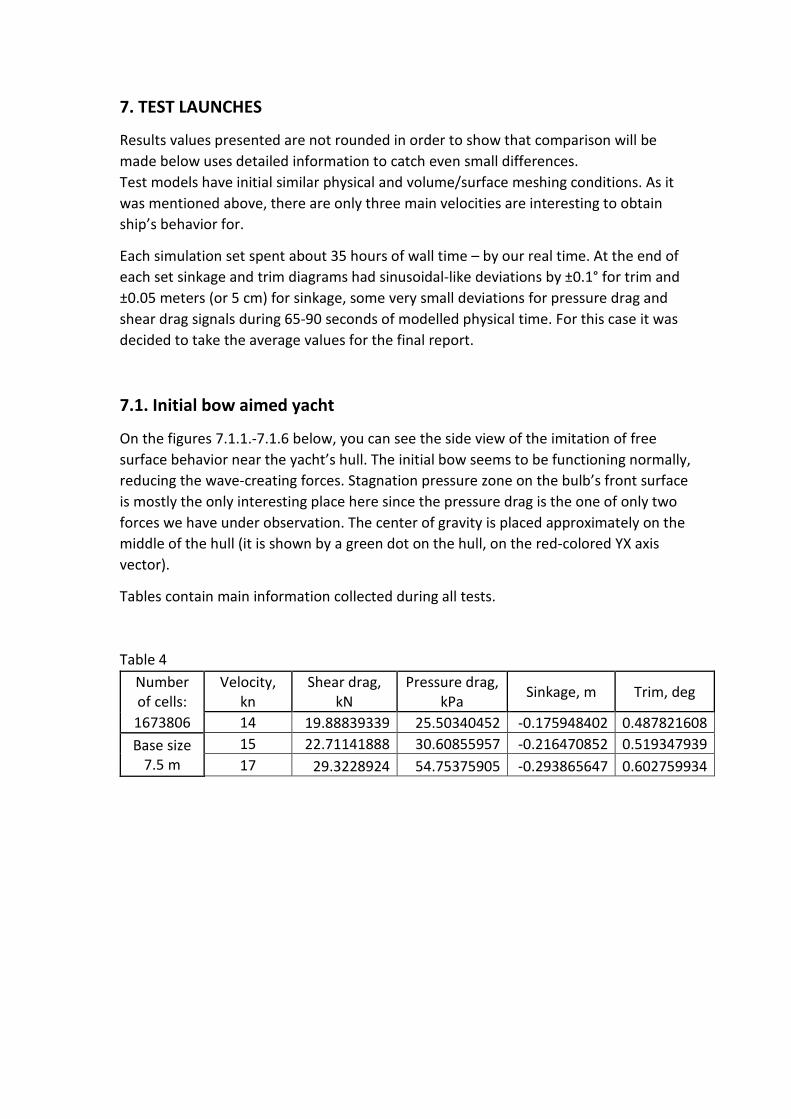
7. TEST LAUNCHES
Results values presented are not rounded in order to show that comparison will be
made below uses detailed information to catch even small differences.
Test models have initial similar physical and volume/surface meshing conditions. As it
was mentioned above, there are only three main velocities are interesting to obtain
ship’s behavior for.
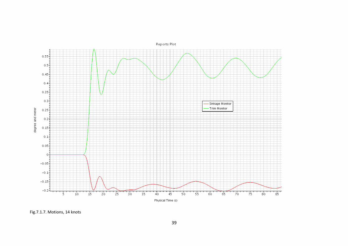
Each simulation set spent about 35 hours of wall time – by our real time. At the end of
each set sinkage and trim diagrams had sinusoidal-like deviations by ±0.1° for trim and
±0.05 meters (or 5 cm) for sinkage, some very small deviations for pressure drag and
shear drag signals during 65-90 seconds of modelled physical time. For this case it was
decided to take the average values for the final report.
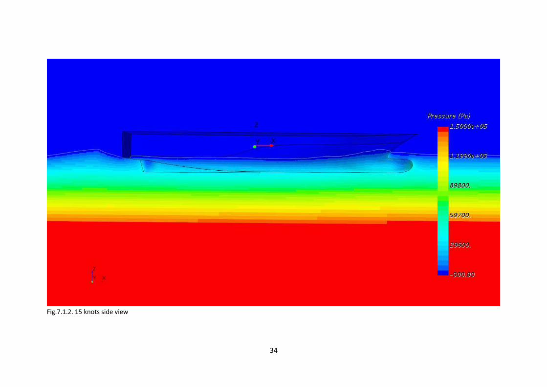
7.1. Initial bow aimed yacht
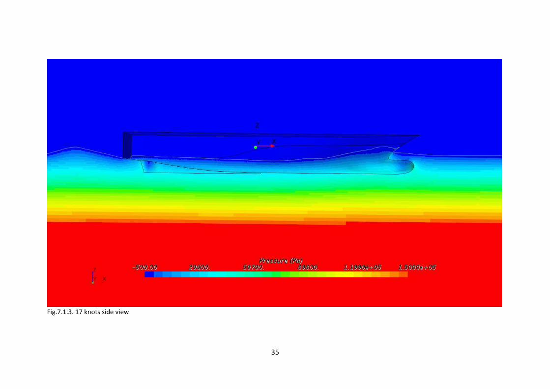
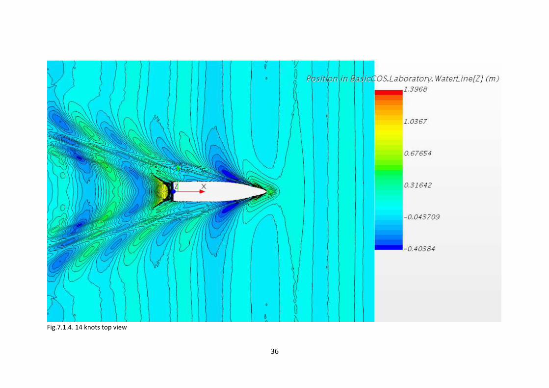
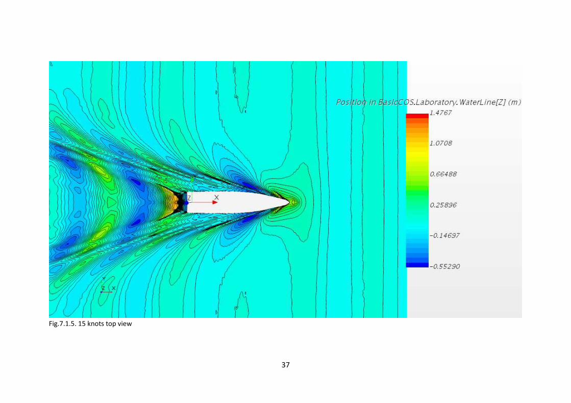
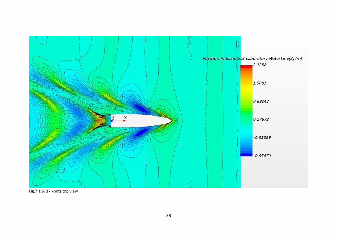
On the figures 7.1.1.-7.1.6 below, you can see the side view of the imitation of free
surface behavior near the yacht’s hull. The initial bow seems to be functioning normally,
reducing the wave-creating forces. Stagnation pressure zone on the bulb’s front surface
is mostly the only interesting place here since the pressure drag is the one of only two
forces we have under observation. The center of gravity is placed approximately on the
middle of the hull (it is shown by a green dot on the hull, on the red-colored YX axis
vector).
Tables contain main information collected during all tests.
Table 4
Number
of cells:
Velocity,
kn
Shear drag,
kN
Pressure drag,
kPa Sinkage, m Trim, deg
1673806 14 19.88839339 25.50340452 -0.175948402 0.487821608
Base size
7.5 m
15 22.71141888 30.60855957 -0.216470852 0.519347939
17 29.3228924 54.75375905 -0.293865647 0.602759934

The subject of interest. Bulbous bow.
Fig.7.1.1. 14 knots side view
This light-colored line is a
profile of water free surface
34
Fig.7.1.2. 15 knots side view
35
Fig.7.1.3. 17 knots side view
36
Fig.7.1.4. 14 knots top view
37
Fig.7.1.5. 15 knots top view
38
Fig.7.1.6. 17 knots top view
39
Fig.7.1.7. Motions, 14 knots
40
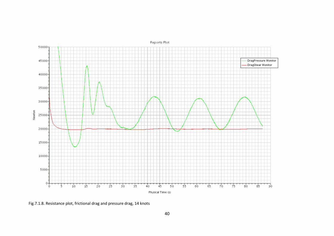
Fig.7.1.8. Resistance plot, frictional drag and pressure drag, 14 knots

41
Fig.7.1.9. Motions, 15 knots
42
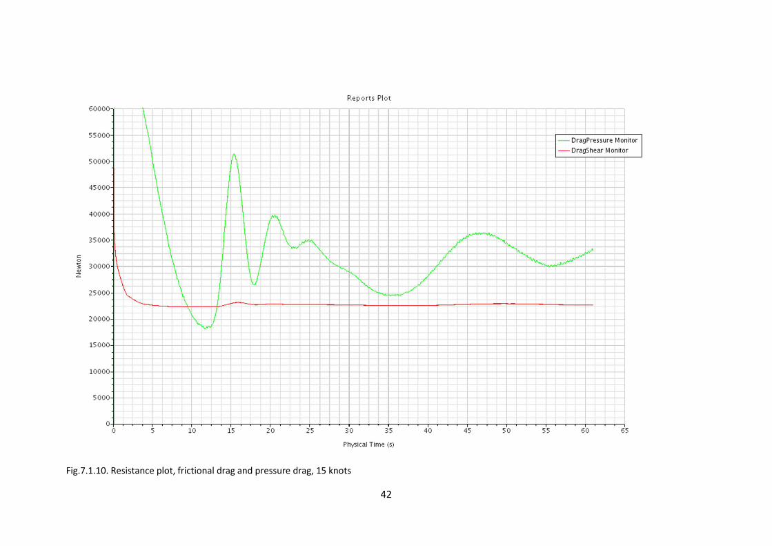
Fig.7.1.10. Resistance plot, frictional drag and pressure drag, 15 knots
43
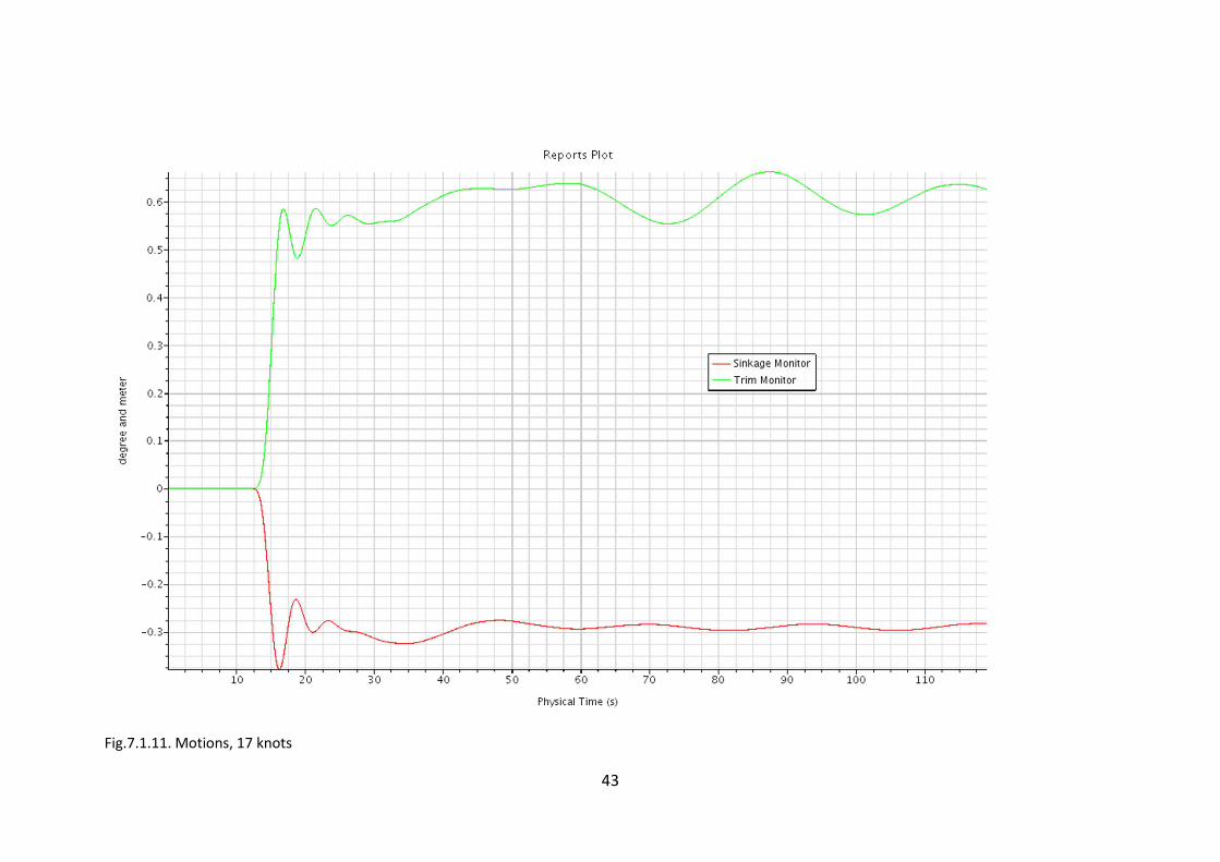
Fig.7.1.11. Motions, 17 knots
44
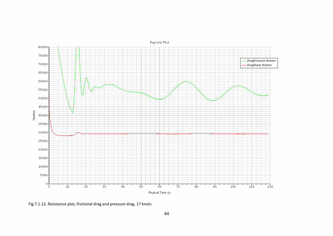
Fig.7.1.12. Resistance plot, frictional drag and pressure drag, 17 knots
45
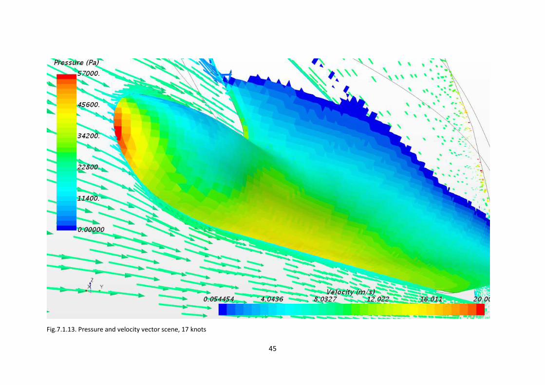
Fig.7.1.13. Pressure and velocity vector scene, 17 knots
46
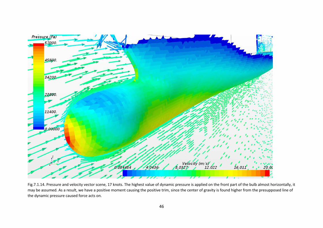
Fig.7.1.14. Pressure and velocity vector scene, 17 knots. The highest value of dynamic pressure is applied on the front part of the bulb almost horizontally, it
may be assumed. As a result, we have a positive moment causing the positive trim, since the center of gravity is found higher from the presupposed line of
the dynamic pressure caused force acts on.
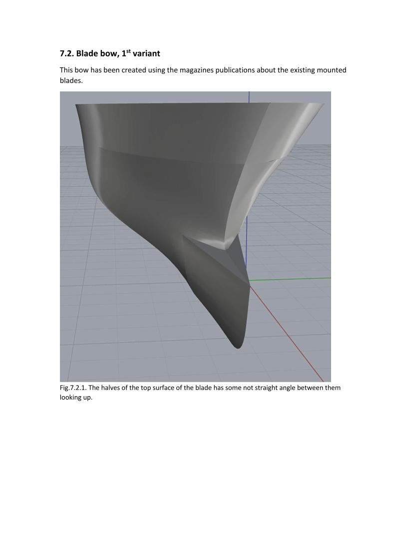
7.2. Blade bow, 1st variant
This bow has been created using the magazines publications about the existing mounted
blades.
Fig.7.2.1. The halves of the top surface of the blade has some not straight angle between them
looking up.
48
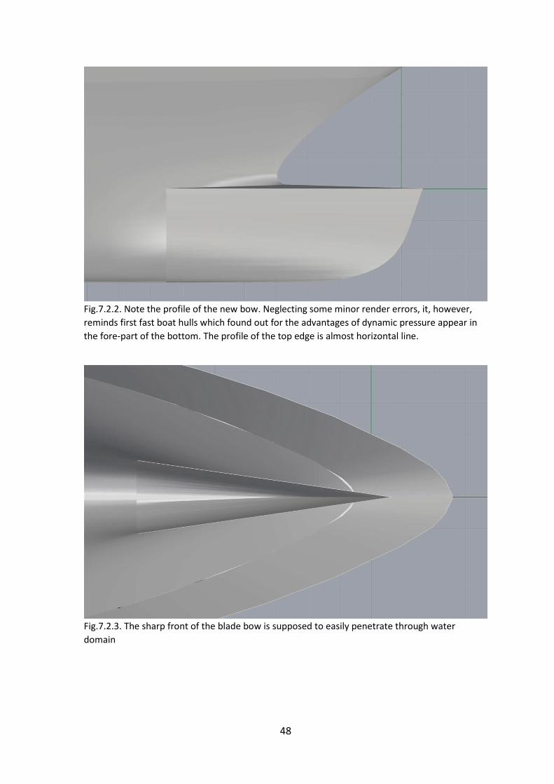
Fig.7.2.2. Note the profile of the new bow. Neglecting some minor render errors, it, however,
reminds first fast boat hulls which found out for the advantages of dynamic pressure appear in
the fore-part of the bottom. The profile of the top edge is almost horizontal line.
Fig.7.2.3. The sharp front of the blade bow is supposed to easily penetrate through water
domain
49
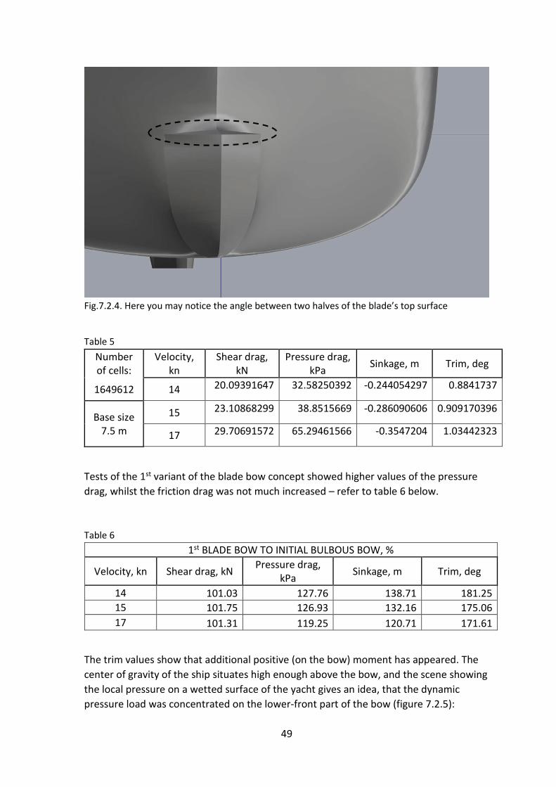
Fig.7.2.4. Here you may notice the angle between two halves of the blade’s top surface
Table 5
Number
of cells:
Velocity,
kn
Shear drag,
kN
Pressure drag,
kPa Sinkage, m Trim, deg
1649612 14 20.09391647 32.58250392 -0.244054297 0.8841737
Base size
7.5 m
15 23.10868299 38.8515669 -0.286090606 0.909170396
17 29.70691572 65.29461566 -0.3547204 1.03442323
Tests of the 1st variant of the blade bow concept showed higher values of the pressure
drag, whilst the friction drag was not much increased – refer to table 6 below.
Table 6
1st BLADE BOW TO INITIAL BULBOUS BOW, %
Velocity, kn Shear drag, kN Pressure drag,
kPa Sinkage, m Trim, deg
14 101.03 127.76 138.71 181.25
15 101.75 126.93 132.16 175.06
17 101.31 119.25 120.71 171.61
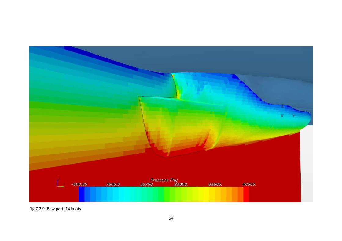
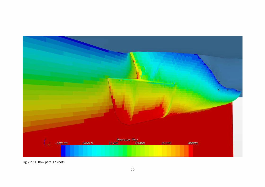
The trim values show that additional positive (on the bow) moment has appeared. The
center of gravity of the ship situates high enough above the bow, and the scene showing
the local pressure on a wetted surface of the yacht gives an idea, that the dynamic
pressure load was concentrated on the lower-front part of the bow (figure 7.2.5):
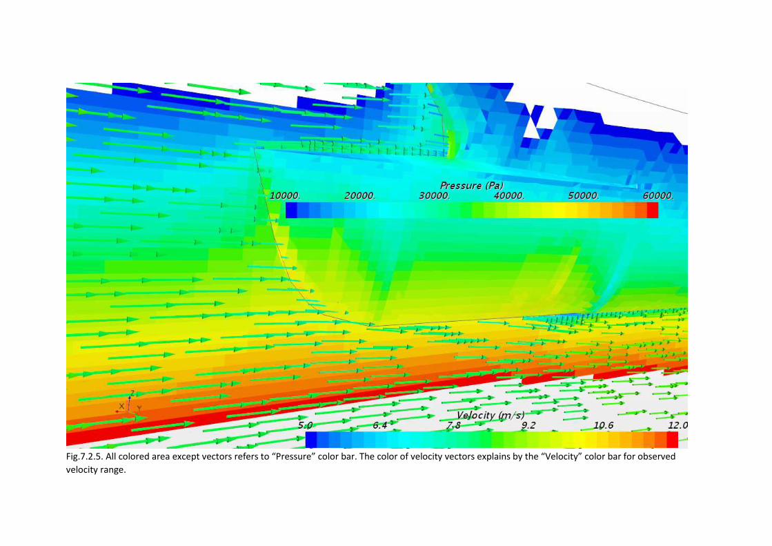
Fig.7.2.5. All colored area except vectors refers to “Pressure” color bar. The color of velocity vectors explains by the “Velocity” color bar for observed
velocity range.
51
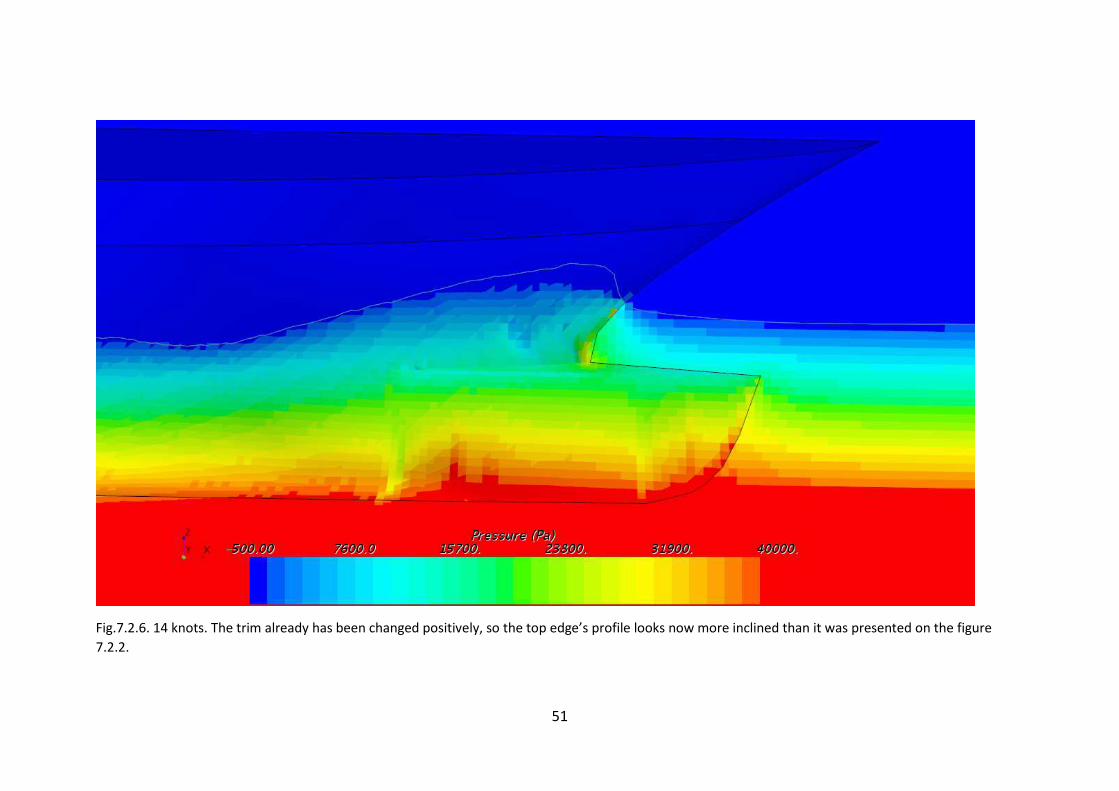
Fig.7.2.6. 14 knots. The trim already has been changed positively, so the top edge’s profile looks now more inclined than it was presented on the figure
7.2.2.
52
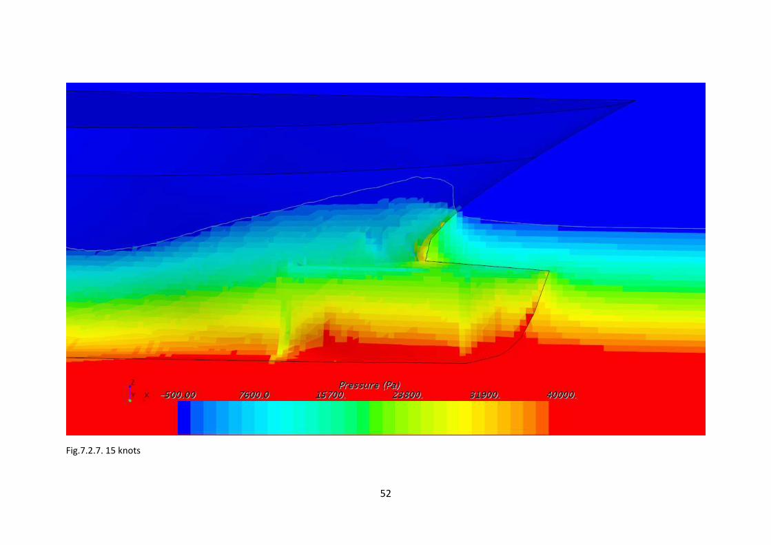
Fig.7.2.7. 15 knots
53
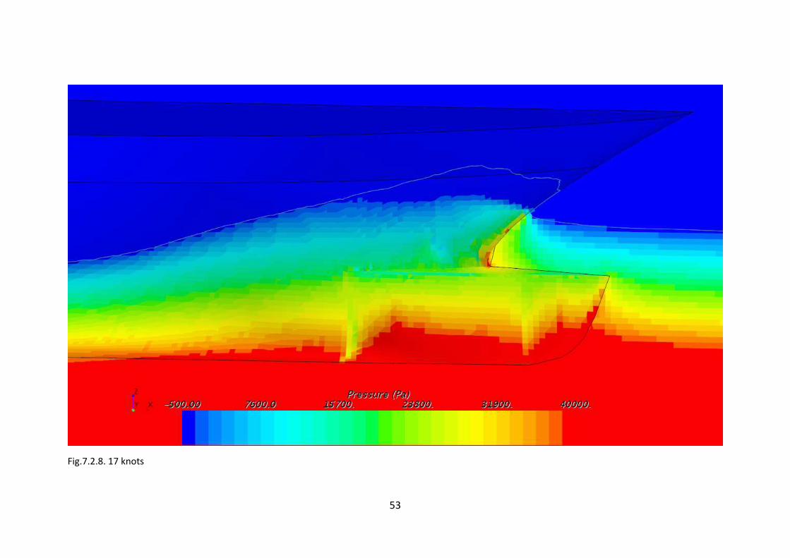
Fig.7.2.8. 17 knots
54
Fig.7.2.9. Bow part, 14 knots
55
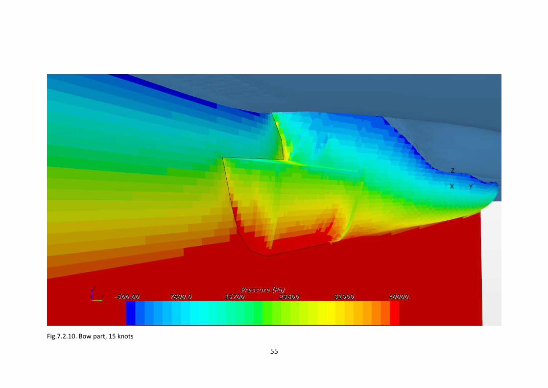
Fig.7.2.10. Bow part, 15 knots
56
Fig.7.2.11. Bow part, 17 knots
57
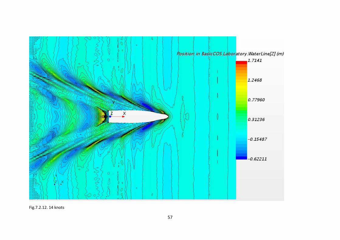
Fig.7.2.12. 14 knots
58
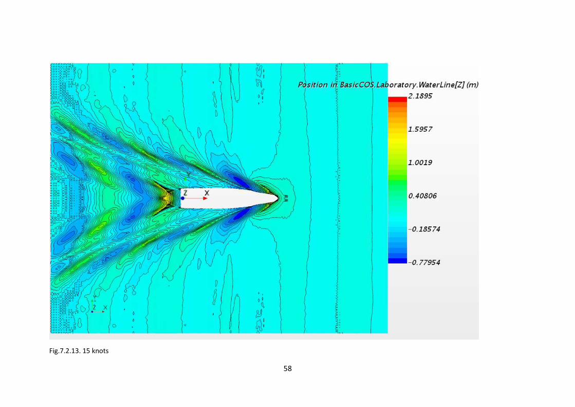
Fig.7.2.13. 15 knots
59
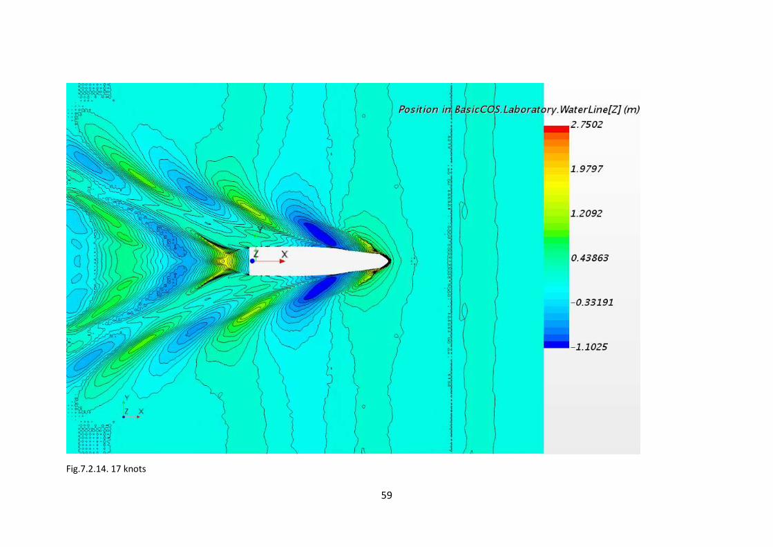
Fig.7.2.14. 17 knots
60
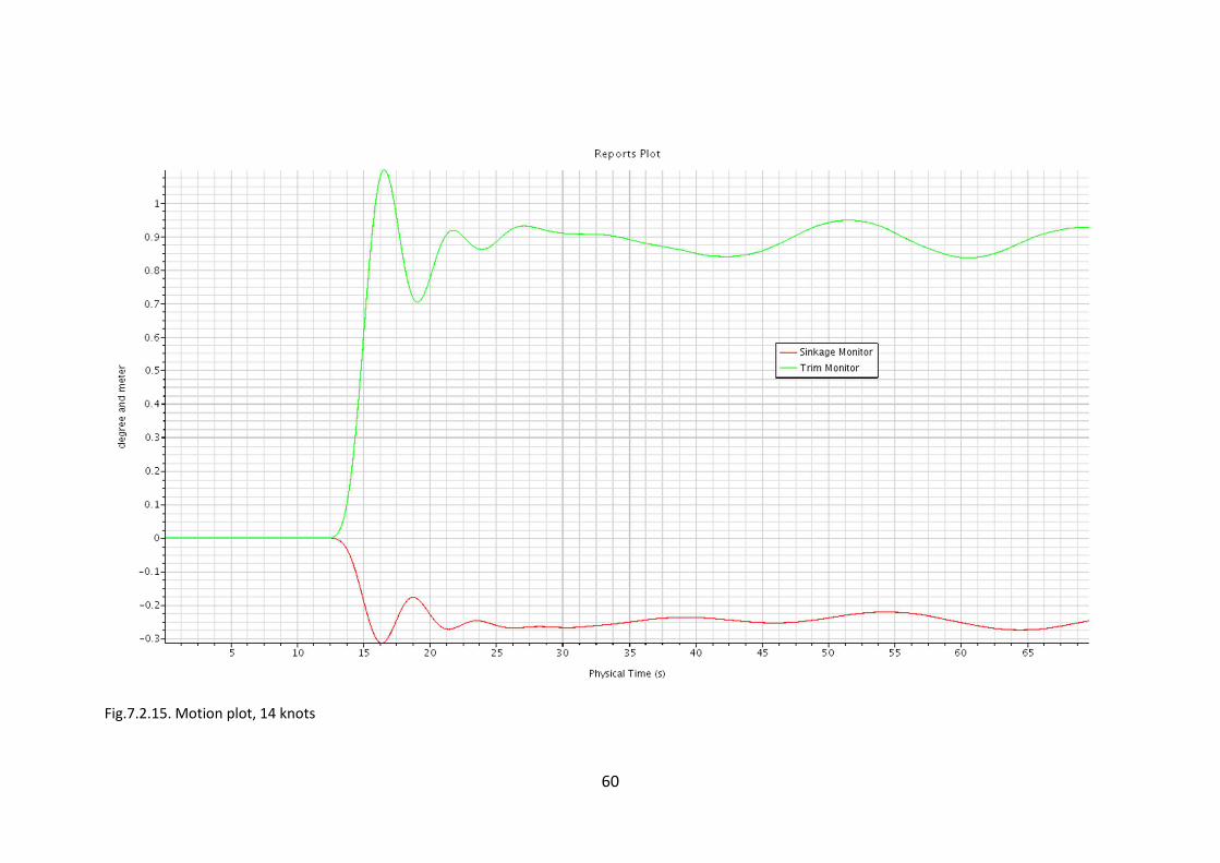
Fig.7.2.15. Motion plot, 14 knots
61
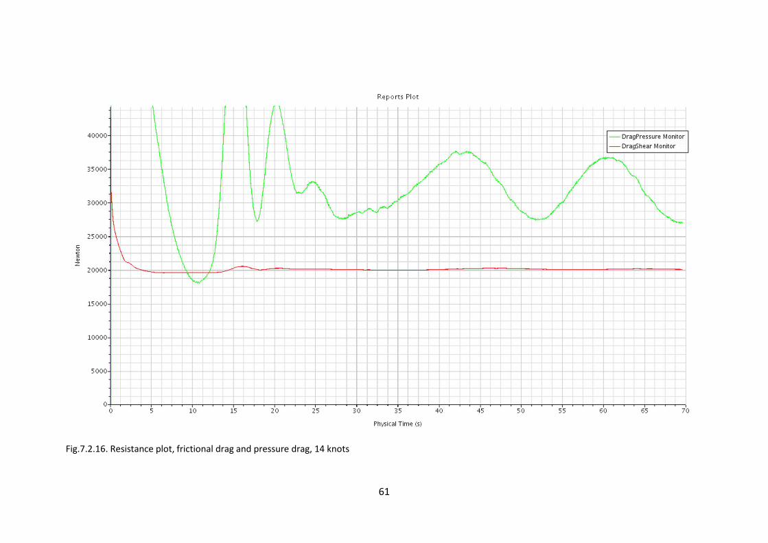
Fig.7.2.16. Resistance plot, frictional drag and pressure drag, 14 knots
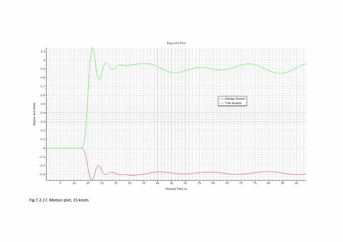
Fig.7.2.17. Motion plot, 15 knots
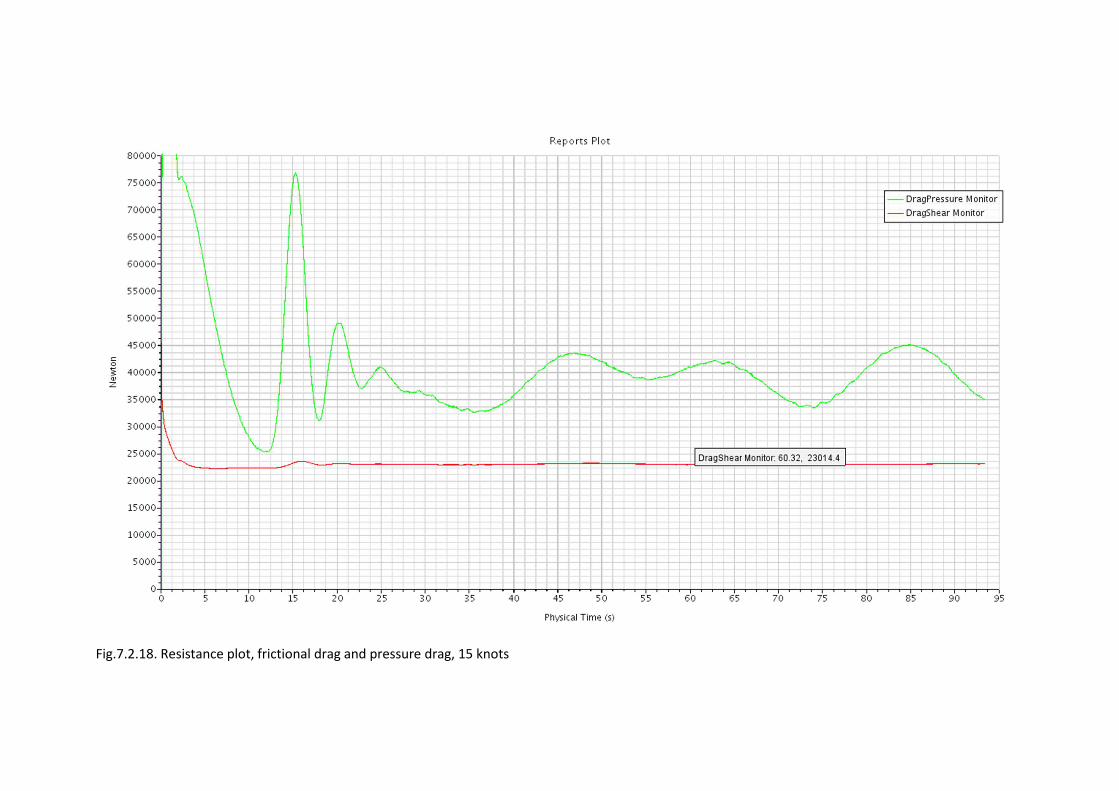
Fig.7.2.18. Resistance plot, frictional drag and pressure drag, 15 knots
64
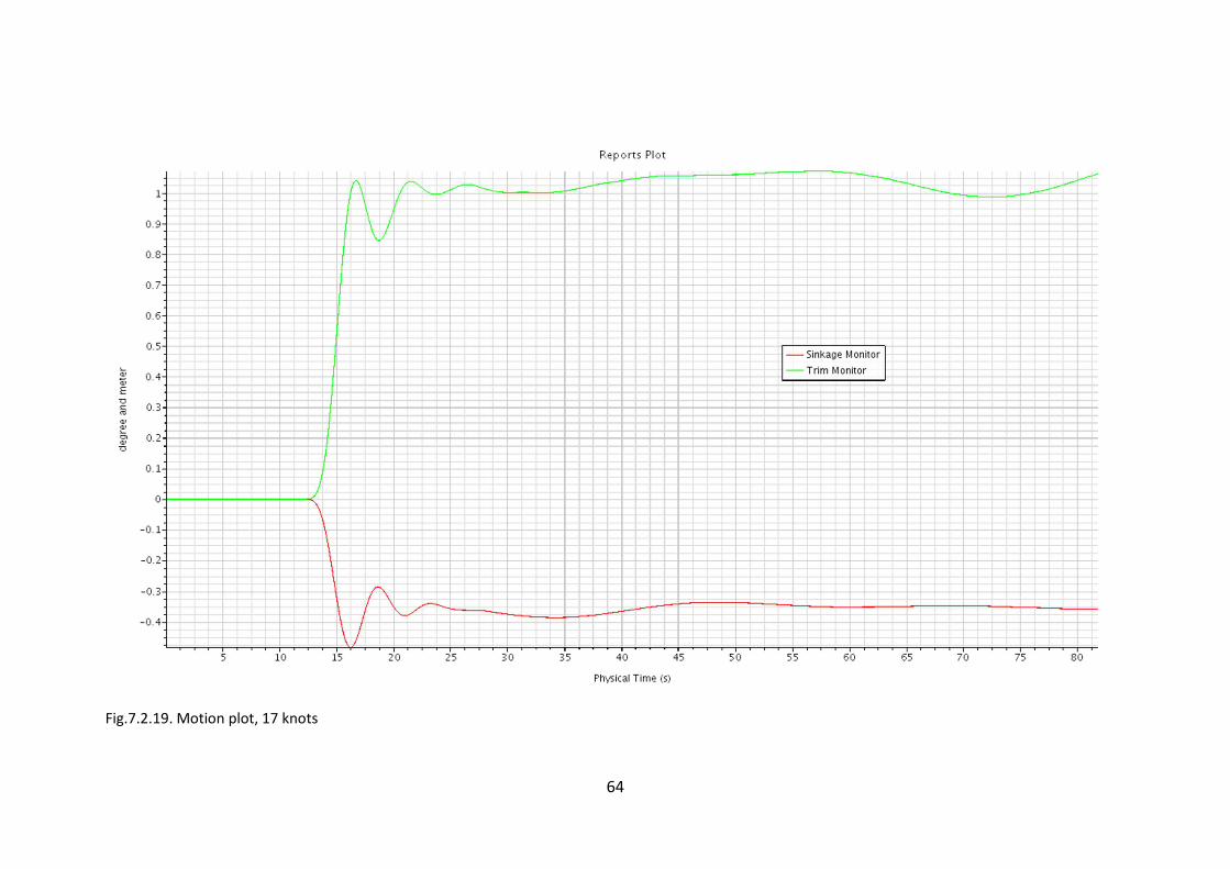
Fig.7.2.19. Motion plot, 17 knots

Fig.7.2.20. Resistance plot, frictional drag and pressure drag, 17 knots
66
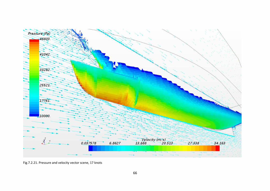
Fig.7.2.21. Pressure and velocity vector scene, 17 knots
67
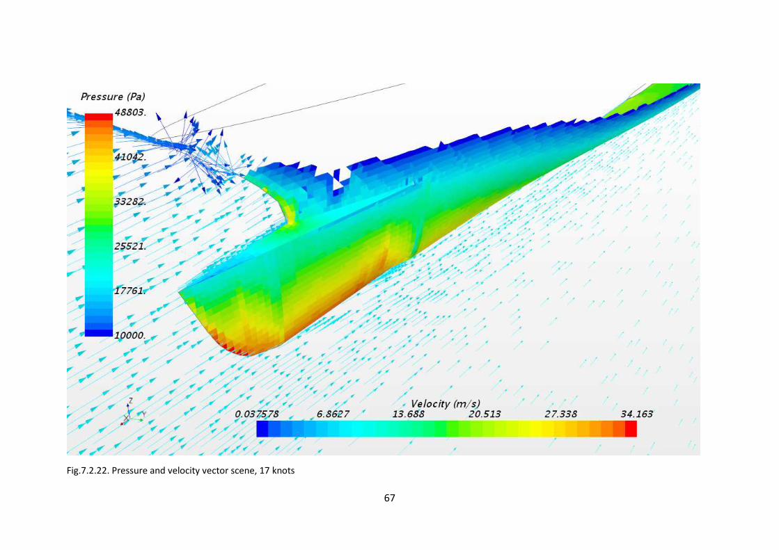
Fig.7.2.22. Pressure and velocity vector scene, 17 knots
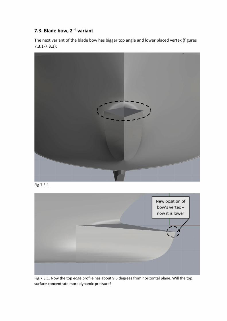
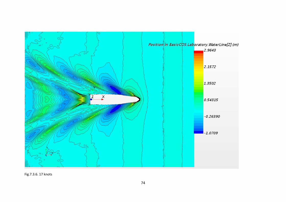
7.3. Blade bow, 2nd variant
The next variant of the blade bow has bigger top angle and lower placed vertex (figures
7.3.1-7.3.3):
Fig.7.3.1
Fig.7.3.1. Now the top edge profile has about 9.5 degrees from horizontal plane. Will the top
surface concentrate more dynamic pressure?
New position of
bow’s vertex –
now it is lower
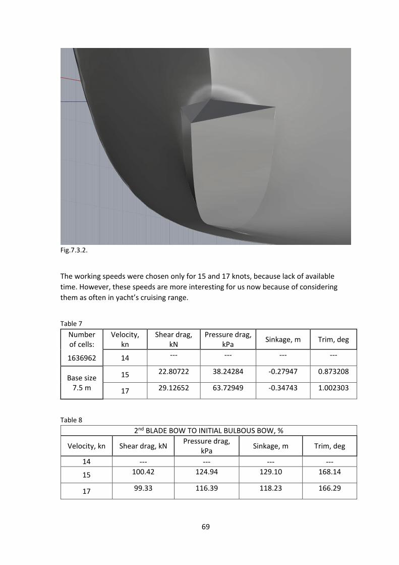
69
Fig.7.3.2.
The working speeds were chosen only for 15 and 17 knots, because lack of available
time. However, these speeds are more interesting for us now because of considering
them as often in yacht’s cruising range.
Table 7
Number
of cells:
Velocity,
kn
Shear drag,
kN
Pressure drag,
kPa Sinkage, m Trim, deg
1636962 14 --- --- --- ---
Base size
7.5 m
15 22.80722 38.24284 -0.27947 0.873208
17 29.12652 63.72949 -0.34743 1.002303
Table 8
2nd BLADE BOW TO INITIAL BULBOUS BOW, %
Velocity, kn Shear drag, kN Pressure drag,
kPa Sinkage, m Trim, deg
14 --- --- --- ---
15 100.42 124.94 129.10 168.14
17 99.33 116.39 118.23 166.29

70
Comparing the tables 6 and 8, it could be noted that the second variant of the “blade”
has better performance than the first one. The shear drag values in this case are almost
the same with the results for the initial bow. Pressure drag on 17 knots also less. Trim
and sinkage differ from the results for the first “blade” being closer to the motions when
aiming the initial bulb. The trim angle and sinkage had been reduced.
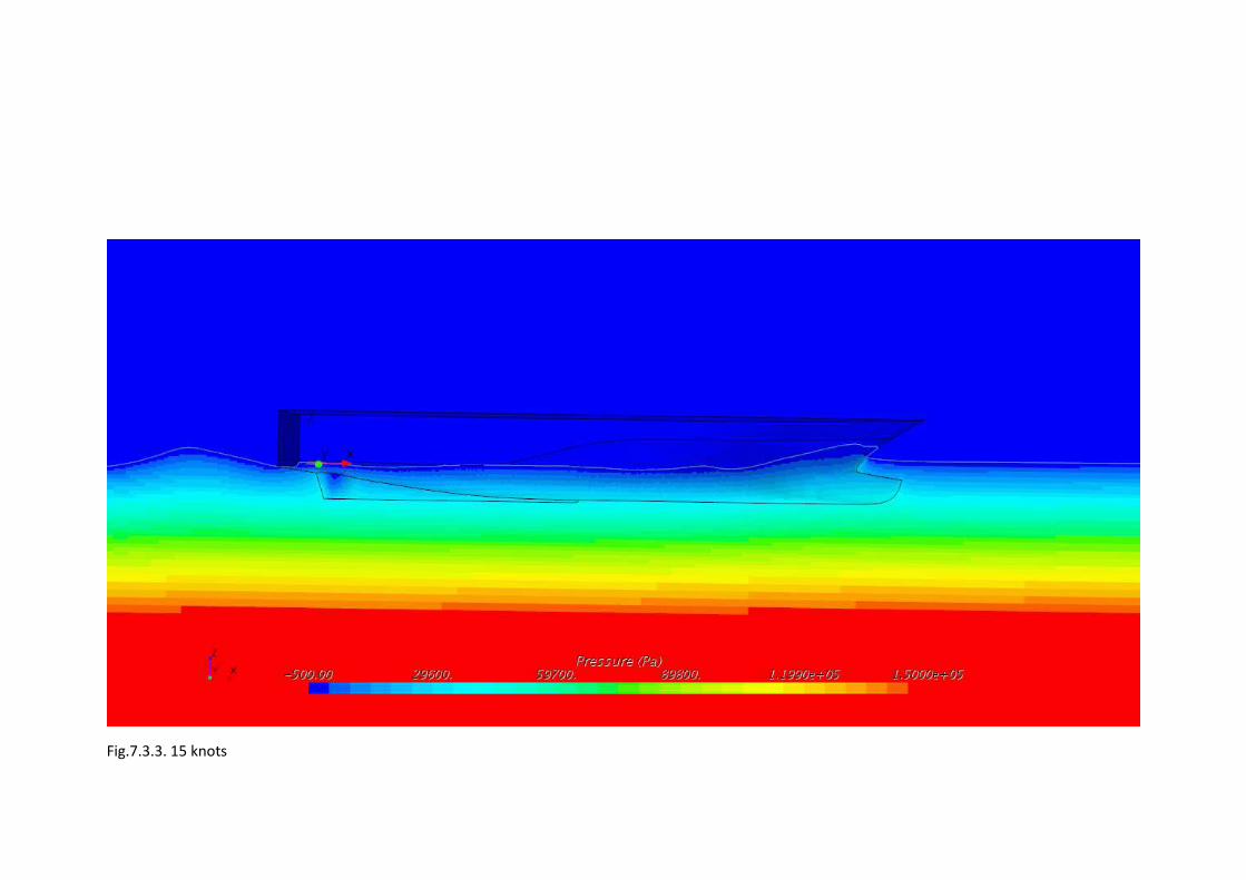
Fig.7.3.3. 15 knots
72
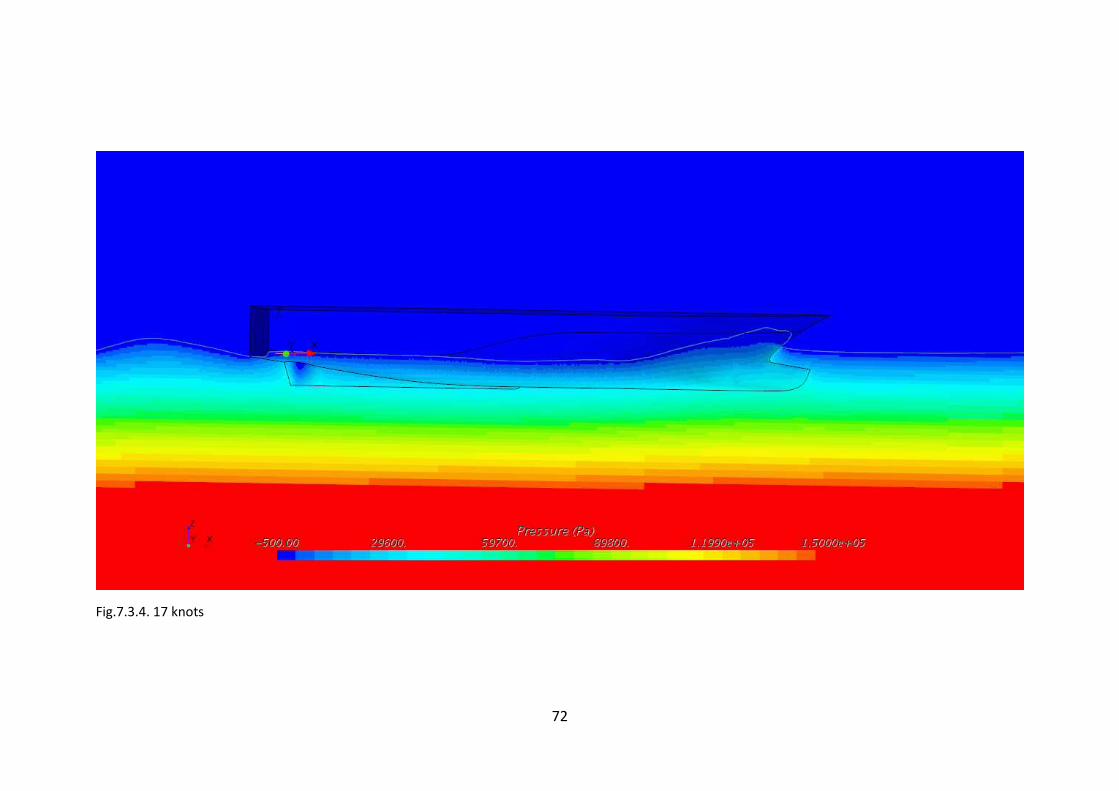
Fig.7.3.4. 17 knots
73
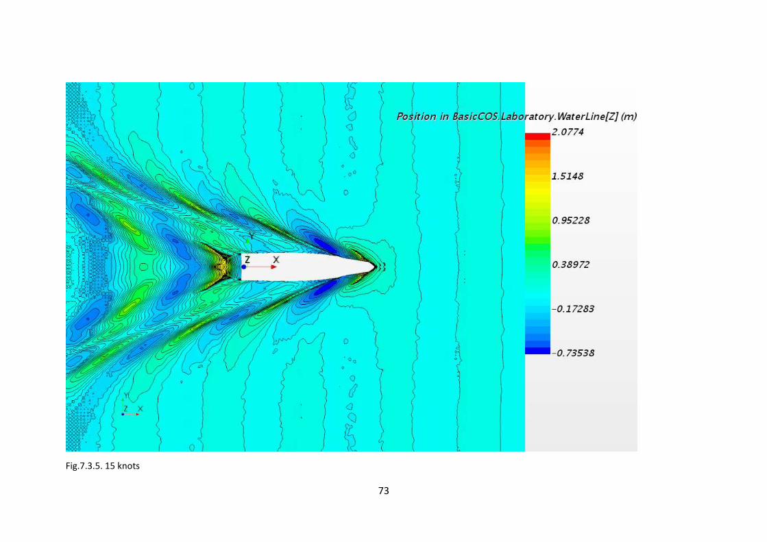
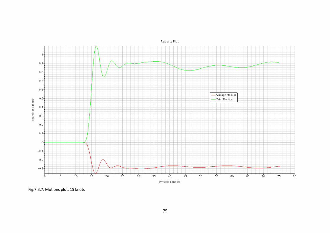
Fig.7.3.5. 15 knots
74
Fig.7.3.6. 17 knots
75
Fig.7.3.7. Motions plot, 15 knots
76
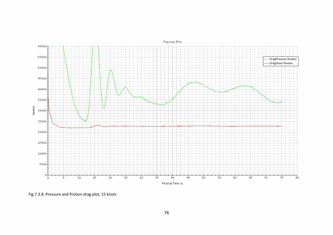
Fig.7.3.8. Pressure and friction drag plot, 15 knots
77
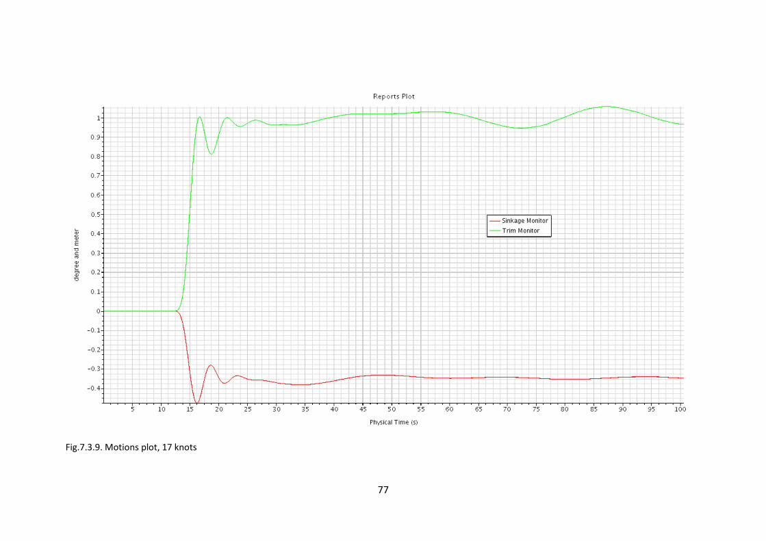
Fig.7.3.9. Motions plot, 17 knots
78
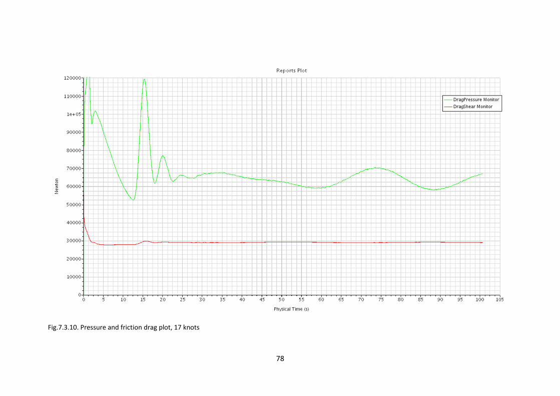
Fig.7.3.10. Pressure and friction drag plot, 17 knots
79
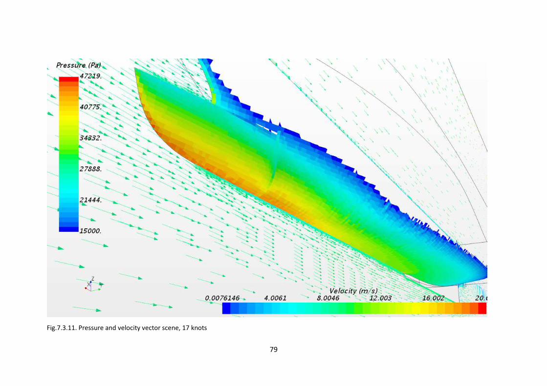
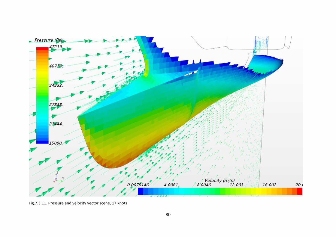
Fig.7.3.11. Pressure and velocity vector scene, 17 knots
80
Fig.7.3.11. Pressure and velocity vector scene, 17 knots
81
CONCLUSION
The results for the new bows shows that the question of application of the blade bow’s
concept must be researched deeply, since the change of the only one feature – blade’s
top surface inclination – may sensibly change the values of the resistance and
seakeeping behavior of the ship.
The pressure drag increases much when switching from convenient bow to the blade
one. But it was noticed, that the value of the pressure drag excess percentage decreases
by 7-8% if the yacht’s velocity increases. This fact must be noted.
Paying attention on the wave height produced by yacht in fore-part: the height has been
increased by almost 30-40%. The blade bows did not function like the bulbous one
crushing the incoming wave. In the test cases the initial water surface was flat, even
having a velocity directed in oppositely to the ship, however, wave producing aspect
should be noticed as well. Important changes to be noted:
1) Pressure drag decreases with speed increasing;
2) Friction drag does not changes much;
3) Trim and sinkage already may be much enough dependent of bow’s only one
feature has been modified.
The author suggests this problem to be referred to the problem of shape optimization
for the first stage of future research. There are some more ideas for the new bow forms
ready to be checked on the presented yacht hull without deforming the rest part of it
different from the already changed bow part areas. The very first significant factor
influencing the way of bow shape modification refers to production issues – 60 meters-
long fully displacement yacht with convex shape lines is hard to be changed for the same
way as it was done for Ilumen 28M and Benetti F-125 without having huge undefined
yet effect on the main hull hydrodynamics.
The concept of blade bow is relatively new, a lot of potential benefits may be found
after digging the subject deeper. Some of them already has shown themselves: for
example, the trim and sinkage changing patterns depend on some particular features of
the bow – good starting point for the parametrical design study.
Hence, the future research might be initiated should include, at least, parametrical
design study and bow shape optimization works in order to clarify:
a) what minimum number of geometrical parameters of the blade bow may be
modified in order to affect seakeeping patterns in a way needed;
b) optimization of the bow for different types of vessels using already defined
parameters from the parametrical design study.
The work is recommended to be continued.

82
REFERENCES
1. Gemma Fottles, “Dominator Ilumen 28M taking shape in Italy”, web-article, 11th
April 2016, electronic magazine “Superyacht”, link to the article:
https://www.superyachttimes.com/yacht-news/dominator-ilumen-28m-taking-
shape-in-italy
2. Michael Verdon, “Dominator’s Ilumen Is Now More Spacious and Preparing for
Launch”, web-article, 13th April 2016, electronic magazine “Robb Report”, link to
the article: http://robbreport.com/motors/marine/dominators-ilumen-now-
more-spacious-and-preparing-launch-231479/
3. “Benetti NEWS from the yard November – December 2013”, web-article, 16th
December 2013, electronic magazine “Sand People Communication”, link to the
article: https://sandpeoplecommunication.wordpress.com/2013/12/16/benetti-
news-from-the-yard-november-december-2013
4. Marco Ferrando, Lecture notes in Motor Yacht Design, Master of Science course
in Yacht Design,
5. Ilumen 28M brochure from Web-site of the Derani Yachts Co. Ltd.
(https://www.derani-yachts.com/yachts/dominator-ilumen-28-metre/#)
6. Giuliano Sargentini, http://www.sargentinifoto.it/
7. http://benettiyachts.it/fast-125/
8. https://www.pressreader.com/italy/superyacht/20170109/282428463876372
9. https://www.pressreader.com/italy/superyacht/20170109/282398399105300
10. “Semicustom with a Sporty Spirit”, web-article, 16th September 2013, electronic
magazine “Yachting”, link to the article:
https://www.yachtingmagazine.com/semicustom-sporty-spirit
11. STAR-CCM+ ver.11, User manual
12. Benetti F-125 page in brochure, http://www.navis-
yachts.be/files/65381/Brochure%20Class%20Fast%20Displacement%20Web.pdf
13. “The curious incisive “nose” on new high-speed superyachts”, 9th January 2017,
electronic magazine “Superyacht”
14. Joe Banks, A.B. Phillips, Stephen R. Turnock, Southampton University. Free-
surface CFD Prediction of Components of Ship Resistance for KCS
15. C.A. Perez G, M. Tan, P.A. Wilson. VALIDATION AND VERIFICATION OF HULL
RESISTANCE COMPONENTS USING A COMMERCIAL CFD CODE