Design Of Fuzzy Controllers

Jan Jantzen jj@iau.dtu.dk:1

$EVWUDFWDesign of a fuzzy controller requires more design decisions than usual, for example

regarding rule base, inference engine, defuzzification, and data pre- and post processing.This tutorial paper identifies and describes the design choices related to single-loop fuzzycontrol, based on an international standard which is underway. The paper contains also adesign approach, which uses a PID controller as a starting point. A design engineer canview the paper as an introduction to fuzzy controller design.

&RQWHQWV

� ,QWURGXFWLRQ �

� 6WUXFWXUH RI D IX]]\ FRQWUROOHU �2.1 Preprocessing 62.2 Fuzzification 72.3 Rule Base 72.4 Inference Engine 132.5 Defuzzification 152.6 Postprocessing 16

� 7DEOH %DVHG &RQWUROOHU ��

� ,QSXW�2XWSXW 0DSSLQJ ��

� 7DNDJL�6XJHQR 7\SH &RQWUROOHU ��

� 6XPPDU\ ��

$ $GGLWLYH 5XOH %DVH ��

� Technical University of Denmark, Department of Automation, Bldg 326, DK-2800 Lyngby, DENMARK.Tech. report no 98-E 864 (design), 19 Aug 1998.

1

�� ,QWURGXFWLRQ

While it is relatively easy to design a PID controller, the inclusion of fuzzy rules createsmany extra design problems, and although many introductory textbooks explain fuzzy con-trol, there are few general guidelines for setting the parameters of a simple fuzzy controller.The approach here is based on a three step design procedure, that builds on PID control:

1. Start with a PID controller.2. Insert an equivalent, linear fuzzy controller.3. Make it gradually nonlinear.

Guidelines related to the different components of the fuzzy controller will be intro-duced shortly. In the next three sections three simple realisations of fuzzy controllers aredescribed: a table-based controller, an input-output mapping and a Takagi-Sugeno typecontroller. A short section summarises the main design choices in a simple fuzzy controllerby introducing a check list. The terminology is based on an international standard which isunderway (IEC, 1996).

Fuzzy controllers are used to control consumer products, such as washing machines,video cameras, and rice cookers, as well as industrial processes, such as cement kilns,underground trains, and robots. Fuzzy control is a control method based on fuzzy logic.Just as fuzzy logic can be described simply as ’’computing with words rather than numbers’’,fuzzy control can be described simply as ’’control with sentences rather than equations’’.A fuzzy controller can include empirical rules, and that is especially useful in operatorcontrolled plants.

Take for instance a typical fuzzy controller

1. If error is Neg and change in error is Neg then output is NB

2. If error is Neg and change in error is Zero then output is NM (1)

� � �The collection of rules is called aUXOH EDVH. The rules are in the familiar if-then format, andformally the if-side is called theFRQGLWLRQ and the then-side is called theFRQFOXVLRQ (moreoften, perhaps, the pair is calledDQWHFHGHQW - FRQVHTXHQW or SUHPLVH - FRQFOXVLRQ ). Theinput value ’’Neg’’ is aOLQJXLVWLF WHUP short for the word1HJDWLYH� the output value ’’NB’’stands for1HJDWLYH %LJ and ’’NM’’ for 1HJDWLYH 0HGLXP. The computer is able to executethe rules and compute a control signal depending on the measured inputsHUURU andFKDQJHLQ HUURU.

The objective here is to identify and explain the various design choices for engineers.In a rule based controller the control strategy is stored in a more or less natural language.

The control strategy is isolated in a rule base opposed to an equation based description. Arule based controller is easy to understand and easy to maintain for a non-specialist end-user.An equivalent controller could be implemented using conventional techniques� in fact,any rule based controller could be emulated in, say,)RUWUDQ � it is just that it is convenient

2

Deviations Actions OutputsRef

Controller

End-user

Inferenceengine

Rulebase

Process

Figure 1: Direct control.

to isolate the control strategy in a rule base for operator controlled systems.Fuzzy controllers are being used in various control schemes (IEC, 1996). The most

obvious one is GLUHFW FRQWURO, where the fuzzy controller is in the forward path in a feedbackcontrol system (Fig. 1). The process output is compared with a reference, and if there isa deviation, the controller takes action according to the control strategy. In the figure, thearrows may be understood as hyper-arrows containing several signals at a time for multi-loop control. The sub-components in the figure will be explained shortly. The controller ishere a fuzzy controller, and it replaces a conventional controller, say, a 3,' (proportional-integral-derivative) controller.

In IHHGIRUZDUG FRQWURO (Fig. 2) a measurable disturbance is being compensated. It re-quires a good model, but if a mathematical model is difficult or expensive to obtain, a fuzzymodel may be useful. Figure 2 shows a controller and the fuzzy compensator, the processand the feedback loop are omitted for clarity. The scheme, disregarding the disturbance in-put, can be viewed as a collaboration of linear and nonlinear control actions; the controllerC may be a linear PID controller, while the fuzzy controller F is a supplementary nonlinearcontroller

Fuzzy rules are also used to correct tuning parameters in SDUDPHWHU DGDSWLYH FRQWUROschemes (Fig. 3). If a nonlinear plant changes operating point, it may be possible tochange the parameters of the controller according to each operating point. This is calledJDLQ VFKHGXOLQJ since it was originally used to change process gains. A gain schedulingcontroller contains a linear controller whose parameters are changed as a function of theoperating point in a preprogrammed way. It requires thorough knowledge of the plant, butit is often a good way to compensate for nonlinearities and parameter variations. Sensormeasurements are used as VFKHGXOLQJ YDULDEOHV that govern the change of the controllerparameters, often by means of a table look-up.

Whether a fuzzy control design will be stable is a somewhat open question. Stabilityconcerns the system’s ability to converge or stay close to an equilibrium. AVWDEOH linearsystem will converge to the equilibrium asymptotically no matter where the system statevariables start from. It is relatively straight forward to check for stability in linear systems,

3

++

Sum

F

Fuzzy compensator

C

Controller

uDeviation

Disturbance

Figure 2: Feedforward control.

OutputsRef

Controller Process

Fuzzy gain schedule

Controller parameters

Figure 3: Fuzzy parameter adaptive control.

4

for example by checking that all eigenvalues are in the left half of the complex plane. Fornonlinear systems, and fuzzy systems are most often nonlinear, the stability concept is morecomplex. A nonlinear system is said to be DV\PSWRWLFDOO\ VWDEOH if, when it starts close toan equilibrium, it will converge to it. Even if it just stays close to the equilibrium, withoutconverging to it, it is said to be VWDEOH (in the sense of Lyapunov). To check conditions forstability is much more difficult with nonlinear systems, partly because the system behav-iour is also influenced by the signal DPSOLWXGHV apart from the IUHTXHQFLHV. The literatureis somewhat theoretical and interested readers are referred to Driankov, Hellendoorn &Reinfrank (1993) or Passino & Yurkovich (1998). They report on four methods (Lyapunovfunctions, Popov, circle, and conicity), and they give several references to scientific papers.It is characteristic, however, that the methods give rather conservative results, which trans-late into unrealistically small magnitudes of the gain factors in order to guarantee stability.

Another possibility is to approximate the fuzzy controller with a linear controller, andthen apply the conventional linear analysis and design procedures on the approximation. Itseems likely that the stability margins of the nonlinear system would be close in some senseto the stability margins of the linear approximation depending on how close the approxi-mation is. This paper shows how to build such a linear approximation, but the theoreticalbackground is still unexplored.

There are at least four main sources for finding control rules (Takagi & Sugeno in Lee,1990).

� ([SHUW H[SHULHQFH DQG FRQWURO HQJLQHHULQJ NQRZOHGJH� One classical example is theoperator’s handbook for a cement kiln (Holmblad & Ostergaard, 1982). The most com-mon approach to establishing such a collection of rules of thumb, is to question expertsor operators using a carefully organised questionnaire.

� %DVHG RQ WKH RSHUDWRU¶V FRQWURO DFWLRQV� FuzzyLI�WKHQ rules can be deduced from ob-servations of an operator’s control actions or a log book. The rules express input-outputrelationships.

� %DVHG RQ D IX]]\ PRGHO RI WKH SURFHVV� A linguistic rule base may be viewed as aninverse model of the controlled process. Thus the fuzzy control rules might be obtainedby inverting a fuzzy model of the process. This method is restricted to relatively loworder systems, but it provides an explicit solution assuming that fuzzy models of theopen and closed loop systems are available (Braae & Rutherford in Lee, 1990). Anotherapproach isIX]]\ LGHQWLILFDWLRQ (Tong; Takagi & Sugeno; Sugeno – all in Lee, 1990;Pedrycz, 1993) or fuzzy model-based control (see later).

� %DVHG RQ OHDUQLQJ� The self-organising controller is an example of a controller thatfinds the rules itself. Neural networks is another possibility.

There is no design procedure in fuzzy control such as root-locus design, frequency re-sponse design, pole placement design, or stability margins, because the rules are often non-linear. Therefore we will settle for describing the basic components and functions of fuzzycontrollers, in order to recognise and understand the various options in commercial soft-ware packages for fuzzy controller design.

There is much literature on fuzzy control and many commercial software tools (MIT,

5

1995), but there is no agreement on the terminology, which is confusing. There are efforts,however, to standardise the terminology, and the following makes use of a draft of a stan-dard from the International Electrotechnical Committee (IEC, 1996). Throughout, lettersdenoting matrices are in bold upper case, for example $; vectors are in bold lower case,for example [; scalars are in italics, for example Q ; and operations are in bold, for examplePLQ.

�� 6WUXFWXUH RI D IX]]\ FRQWUROOHU

There are specific components characteristic of a fuzzy controller to support a design pro-cedure. In the block diagram in Fig. 4, the controller is between a preprocessing block anda post-processing block. The following explains the diagram block by block.

Fuzzy controller

Inferenceengine

Rulebase Defuzzi-

ficationPostpro-cessing

Fuzzi-fication

Prepro-cessing

Figure 4: Blocks of a fuzzy controller.

��� 3UHSURFHVVLQJ

The inputs are most often hard or FULVS measurements from some measuring equipment,rather than linguistic. A preprocessor, the first block in Fig. 4, conditions the measurementsbefore they enter the controller. Examples of preprocessing are:

� Quantisation in connection with sampling or rounding to integers;� normalisation or scaling onto a particular, standard range;� filtering in order to remove noise;� averaging to obtain long term or short term tendencies;� a combination of several measurements to obtain key indicators; and� differentiation and integration or their discrete equivalences.

A TXDQWLVHU is necessary to convert the incoming values in order to find the best levelin a discrete XQLYHUVH. Assume, for instance, that the variable HUURU has the value 4.5, butthe universe is X @ +�8>�7> = = = > 3> = = = > 7> 8,. The quantiser rounds to 5 to fit it to thenearest level. Quantisation is a means to reduce data, but if the quantisation is too coarsethe controller may oscillate around the reference or even become unstable.

Nonlinear VFDOLQJ is an option (Fig. 5). In the)/6PLGWK controller the operator is asked

6

-5 0 5-100

0

100

input

scal

ed in

put

Figure 5: Example of nonlinear scaling of an input measurement.

to enter three typical numbers for a small, medium and large measurement respectively(Holmblad & Østergaard, 1982). They become break-points on a curve that scales theincoming measurements (circled in the figure). The overall effect can be interpreted as adistortion of the primary fuzzy sets. It can be confusing with both scaling and gain factorsin a controller, and it makes tuning difficult.

When the input to the controller isHUURU, the control strategy is a static mapping betweeninput and control signal. A dynamic controller would have additional inputs, for examplederivatives, integrals, or previous values of measurements backwards in time. These arecreated in the preprocessor thus making the controller multi-dimensional, which requiresmany rules and makes it more difficult to design.

The preprocessor then passes the data on to the controller.

��� )X]]LILFDWLRQ

The first block inside the controller isIX]]LILFDWLRQ, which converts each piece of inputdata to degrees of membership by a lookup in one or several membership functions. Thefuzzification block thus matches the input data with the conditions of the rules to determinehow well the condition of each rule matches that particular input instance. There is a degreeof membership for each linguistic term that applies to that input variable.

��� 5XOH %DVH

The rules may use several variables both in the condition and the conclusion of the rules.The controllers can therefore be applied to both multi-input-multi-output (MIMO) problemsand single-input-single-output (SISO) problems. The typical SISO problem is to regulatea control signal based on an error signal. The controller may actually need both theHUURU,the FKDQJH LQ HUURU, and theDFFXPXODWHG HUURU as inputs, but we will call it single-loopcontrol, because in principle all three are formed from the error measurement. To simplify,this section assumes that the control objective is to regulate some process output around aprescribed setpoint or reference. The presentation is thus limited to single-loop control.

5XOH IRUPDWV Basically a linguistic controller contains rules in theLI�WKHQ format, butthey can be presented in different formats. In many systems, the rules are presented to the

7

end-user in a format similar to the one below,

1. If error is Neg and change in error is Neg then output is NB

2. If error is Neg and change in error is Zero then output is NM

3. If error is Neg and change in error is Pos then output is Zero

4. If error is Zero and change in error is Neg then output is NM

5. If error is Zero and change in error is Zero then output is Zero (2)

6. If error is Zero and change in error is Pos then output is PM

7. If error is Pos and change in error is Neg then output is Zero

8. If error is Pos and change in error is Zero then output is PM

9. If error is Pos and change in error is Pos then output is PB

The names =HUR, 3RV, 1HJ are labels of fuzzy sets as well as 1%, 10, 3% and 30(negative big, negative medium, positive big, and positive medium respectively). The sameset of rules could be presented in a UHODWLRQDO format, a more compact representation.

Error Change in error OutputNeg Pos ZeroNeg Zero NMNeg Neg NBZero Pos PMZero Zero ZeroZero Neg NMPos Pos PBPos Zero PMPos Neg Zero

(3)

The top row is the heading, with the names of the variables. It is understood that the twoleftmost columns are inputs, the rightmost is the output, and each row represents a rule.This format is perhaps better suited for an experienced user who wants to get an overviewof the rule base quickly. The relational format is certainly suited for storing in a relationaldatabase. It should be emphasised, though, that the relational format implicitly assumes thatthe connective between the inputs is always logical DQG � or logical RU for that matter aslong as it is the same operation for all rules � and not a mixture of connectives. Incidentally,a fuzzy rule with an RU combination of terms can be converted into an equivalent DQGcombination of terms using laws of logic (DeMorgan’s laws among others). A third formatis the tabular linguistic format.

Change in errorNeg Zero Pos

Neg NB NM ZeroError Zero NM Zero PM

Pos Zero PM PB

(4)

This is even more compact. The input variables are laid out along the axes, and the outputvariable is inside the table. In case the table has an empty cell, it is an indication of a missing

8

rule, and this format is useful for checking completeness. When the input variables are HUURUand FKDQJH LQ HUURU, as they are here, that format is also called a OLQJXLVWLF SKDVH SODQH. Incase there are q A 5 input variables involved, the table grows to an q-dimensional array;rather user-XQ friendly.

To accommodate several outputs, a nested arrangement is conceivable. A rule withseveral outputs could also be broken down into several rules with one output.

Lastly, a graphical format which shows the fuzzy membership curves is also possible(Fig. 7). This graphical user-interface can display the inference process better than theother formats, but takes more space on a monitor.

&RQQHFWLYHV In mathematics, sentences are connected with the words DQG, RU, LI�WKHQ(or LPSOLHV�, and LI DQG RQO\ LI, or modifications with the word QRW. These five are calledFRQQHFWLYHV. It also makes a difference how the connectives are implemented. The mostprominent is probably multiplication for fuzzy DQG instead of minimum. So far most of theexamples have only contained DQG operations, but a rule like ‘‘If error is very neg and notzero or change in error is zero then ...’’ is also possible.

The connectivesDQG andRU are always defined in pairs, for example,

D DQG E @ PLQ +D>E, minimumD RU E @ PD[ +D>E, maximum

orD DQG E @ D � E algebraic productD RU E @ D. E� D � E algebraic or probabilistic sum

(5)

There are other examples (e.g., Zimmermann, 1991,64� 65,, but they are more com-plex.

0RGLILHUV A linguistic PRGLILHU, is an operation that modifies the meaning of a term.For example, in the sentence ‘‘very close to 0’’, the wordYHU\ modifies&ORVH WR � whichis a fuzzy set. A modifier is thus an operation on a fuzzy set. The modifierYHU\ can bedefined as squaring the subsequent membership function, that is

YHU\ D @ D5 (6)

Some examples of other modifiers are

H[WUHPHO\ D @ D6

VOLJKWO\ D @ D4

6

VRPHZKDW D @ PRUHRUOHVV D DQG QRW VOLJKWO\ D

A whole family of modifiers is generated byDs wheres is any power between zero andinfinity. With s @ 4 the modifier could be namedH[DFWO\, because it would suppress allmemberships lower than 1.0.

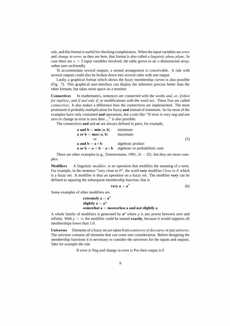
8QLYHUVHV Elements of a fuzzy set are taken from aXQLYHUVH RI GLVFRXUVH or justXQLYHUVH.The universe contains all elements that can come into consideration. Before designing themembership functions it is necessary to consider the universes for the inputs and outputs.Take for example the rule

If error is Neg and change in error is Pos then output is 0

9

Naturally, the membership functions for 1HJ and 3RV must be defined for all possiblevalues of HUURU and FKDQJH LQ HUURU� and a standard universe may be convenient.

Another consideration is whether the input membership functions should be continuousor discrete. A continuous membership function is defined on a continuous universe bymeans of parameters. A discrete membership function is defined in terms of a vector witha finite number of elements. In the latter case it is necessary to specify the range of theuniverse and the value at each point. The choice between fine and coarse resolution is atrade off between accuracy, speed and space demands. The quantiser takes time to execute,and if this time is too precious, continuous membership functions will make the quantiserobsolete.

([DPSOH � �VWDQGDUG XQLYHUVHV� 0DQ\ DXWKRUV DQG VHYHUDO FRPPHUFLDO FRQWUROOHUV XVHVWDQGDUG XQLYHUVHV�

� 7KH )/ 6PLGWK FRQWUROOHU� IRU LQVWDQFH� XVHV WKH UHDO QXPEHU LQWHUYDO ^�4> 4`�� $XWKRUV RI WKH HDUOLHU SDSHUV RQ IX]]\ FRQWURO XVHG WKH LQWHJHUV LQ ^�9> 9`�� $QRWKHU SRVVLELOLW\ LV WKH LQWHUYDO ^�433> 433` FRUUHVSRQGLQJ WR SHUFHQWDJHV RI IXOO

VFDOH�� <HW DQRWKHU LV WKH LQWHJHU UDQJH ^3> 73<8` FRUUHVSRQGLQJ WR WKH RXWSXW IURP D �� ELW

DQDORJ WR GLJLWDO FRQYHUWHU�� $ YDULDQW LV ^�537:> 537;` > ZKHUH WKH LQWHUYDO LV VKLIWHG LQ RUGHU WR DFFRPPRGDWH QHJ�

DWLYH QXPEHUV�

7KH FKRLFH RI GDWDW\SHV PD\ JRYHUQ WKH FKRLFH RI XQLYHUVH� )RU H[DPSOH� WKH YROWDJHUDQJH ^�8> 8` FRXOG EH UHSUHVHQWHG DV DQ LQWHJHU UDQJH ^�83> 83`� RU DV D IORDWLQJ SRLQWUDQJH ^�8=3> 8=3`� D VLJQHG E\WH GDWDW\SH KDV DQ DOORZDEOH LQWHJHU UDQJH ^�45;> 45:`�

A way to exploit the range of the universes better is scaling. If a controller input mostlyuses just one term, the scaling factor can be turned up such that the whole range is used.An advantage is that this allows a standard universe and it eliminates the need for addingmore terms.

0HPEHUVKLS IXQFWLRQV Every element in the universe of discourse is a member of afuzzy set to some grade, maybe even zero. The grade of membership for all its membersdescribes a fuzzy set, such as 1HJ. In fuzzy sets elements are assigned a JUDGH RI PHPEHU�VKLS, such that the transition from membership to non-membership is gradual rather thanabrupt. The set of elements that have a non-zero membership is called the VXSSRUW of thefuzzy set. The function that ties a number to each element { of the universe is called thePHPEHUVKLS IXQFWLRQ �+{,.

The designer is inevitably faced with the question of how to build the term sets. Thereare two specific questions to consider: (i) How does one determine the shape of the sets?and (ii) How many sets are necessary and sufficient? For example, the HUURU in the positioncontroller uses the family of terms 1HJ, =HUR, and 3RV. According to fuzzy set theory thechoice of the shape and width is subjective, but a few rules of thumb apply.

� A term set should be sufficiently wide to allow for noise in the measurement.

10

0

0.5

1

(a) (d) (g) (j)

0

0.5

1

(b) (e) (h) (k)

-100 0 1000

0.5

1

(c)-100 0 100

(f)-100 0 100

(i)-100 0 100

(l)

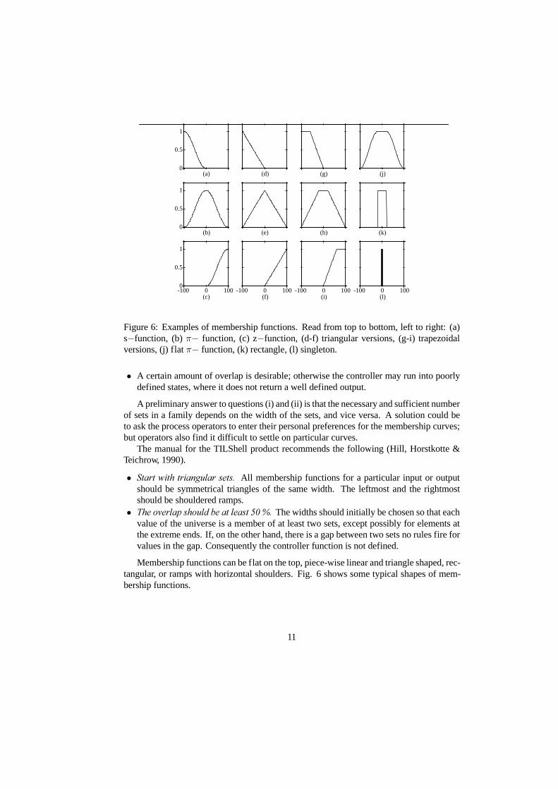
Figure 6: Examples of membership functions. Read from top to bottom, left to right: (a)s�function, (b) �� function, (c) z�function, (d-f) triangular versions, (g-i) trapezoidalversions, (j) flat �� function, (k) rectangle, (l) singleton.

� A certain amount of overlap is desirable; otherwise the controller may run into poorlydefined states, where it does not return a well defined output.

A preliminary answer to questions (i) and (ii) is that the necessary and sufficient numberof sets in a family depends on the width of the sets, and vice versa. A solution could beto ask the process operators to enter their personal preferences for the membership curves;but operators also find it difficult to settle on particular curves.

The manual for the TILShell product recommends the following (Hill, Horstkotte &Teichrow, 1990).

� 6WDUW ZLWK WULDQJXODU VHWV� All membership functions for a particular input or outputshould be symmetrical triangles of the same width. The leftmost and the rightmostshould be shouldered ramps.

� 7KH RYHUODS VKRXOG EH DW OHDVW �� �� The widths should initially be chosen so that eachvalue of the universe is a member of at least two sets, except possibly for elements atthe extreme ends. If, on the other hand, there is a gap between two sets no rules fire forvalues in the gap. Consequently the controller function is not defined.

Membership functions can be flat on the top, piece-wise linear and triangle shaped, rec-tangular, or ramps with horizontal shoulders. Fig. 6 shows some typical shapes of mem-bership functions.

11

Strictly speaking, a fuzzy set D is a collection of ordered pairs

D @ i+{> �+{,,j (7)

Item { belongs to the universe and �+{, is its grade of membership in D. A single pair+{> �+{,, is a fuzzy VLQJOHWRQ ; VLQJOHWRQ RXWSXW means replacing the fuzzy sets in the con-clusion by numbers (scalars). For example

1. If error is Pos then output is 43 volts

2. If error is Zero then output is 3 volts

3. If error is Neg then output is � 43 volts

There are at least three advantages to this:

� The computations are simpler;� it is possible to drive the control signal to its extreme values; and� it may actually be a more intuitive way to write rules.

The scalar can be a fuzzy set with the singleton placed in a proper position. For ex-ample 43 YROWV, would be equivalent to the fuzzy set +3> 3> 3> 3> 4, defined on the universe+�43>�8> 3> 8> 43, YROWV.

([DPSOH � �PHPEHUVKLS IXQFWLRQV� )X]]\ FRQWUROOHUV XVH D YDULHW\ RIPHPEHUVKLS IXQF�WLRQV� $ FRPPRQ H[DPSOH RI D IXQFWLRQ WKDW SURGXFHV D EHOO FXUYH LV EDVHG RQ WKH H[SRQHQ�WLDO IXQFWLRQ�

�+{, @ h{s

��+{� {3,5

5�5

�(8)

7KLV LV D VWDQGDUG *DXVVLDQ FXUYH ZLWK D PD[LPXP YDOXH RI 4� { LV WKH LQGHSHQGHQW YDULDEOHRQ WKH XQLYHUVH� {3 LV WKH SRVLWLRQ RI WKH SHDN UHODWLYH WR WKH XQLYHUVH� DQG � LV WKH VWDQGDUGGHYLDWLRQ� $QRWKHU GHILQLWLRQ ZKLFK GRHV QRW XVH WKH H[SRQHQWLDO LV

�+{, @

%4 .

�{� {3

�

�5&�4

(9)

7KH IO Vplgwk FRQWUROOHU XVHV WKH HTXDWLRQ

�+{, @ 4� h{s

���

�

{3 � {

�d�(10)

7KH H[WUD SDUDPHWHU d FRQWUROV WKH JUDGLHQW RI WKH VORSLQJ VLGHV� ,W LV DOVR SRVVLEOH WR XVHRWKHU IXQFWLRQV� IRU H[DPSOH WKH vljprlg NQRZQ IURP QHXUDO QHWZRUNV�

$ frvlqh IXQFWLRQ FDQ EH XVHG WR JHQHUDWH D YDULHW\ RI PHPEHUVKLS IXQFWLRQV� 7KHv0fxuyh FDQ EH LPSOHPHQWHG DV

v+{o> {u> {, @

;A?A=3 > { ? {o4

5. 4

5frv

�{�{u{u�{o

��

> {o � { � {u

4 > { A {u

<A@A> (11)

ZKHUH {o LV WKH OHIW EUHDNSRLQW� DQG {u LV WKH ULJKW EUHDNSRLQW� 7KH }0fxuyh LV MXVW D UHIOHF�

12

Figure 7: Graphical construction of the control signal in a fuzzy PD controler (generatedin the Matlab Fuzzy Logic Toolbox).

WLRQ�

}+{o> {u> {, @

;A?A=4 > { ? {o4

5. 4

5frv

�{�{o{u�{o

��

> {o � { � {u

3 > { A {u

<A@A> (12)

7KHQ WKH �0fxuyh FDQ EH LPSOHPHQWHG DV D FRPELQDWLRQ RI WKH v0fxuyh DQG WKH }0fxuyh�VXFK WKDW WKH SHDN LV IODW RYHU WKH LQWHUYDO ^{5> {6`

�+{4> {5> {6> {7> {, @ plq+v+{4> {5> {,> }+{6> {7> {,, (13)

��� ,QIHUHQFH (QJLQH

Figures 7 and 8 are both a graphical construction of the algorithm in the core of the con-troller. In Fig. 7, each of the nine rows refers to one rule. For example, the first row saysthat if the HUURU is negative (row 1, column 1) and the FKDQJH LQ HUURU is negative (row1, column 2) then the output should be negative big (row 1, column 3). The picture corre-sponds to the rule base in (2). The rules reflect the strategy that the control signal should bea combination of the reference error and the change in error, a fuzzy proportional-derivativecontroller. We shall refer to that figure in the following. The instances of the HUURU and theFKDQJH LQ HUURU are indicated by the vertical lines on the first and second columns of the

13

chart. For each rule, the inference engine looks up the membership values in the conditionof the rule.

$JJUHJDWLRQ The DJJUHJDWLRQ operation is used when calculating the GHJUHH RI IXOILOO�PHQW or ILULQJ VWUHQJWK �n of the condition of a rule n. A rule, say rule 1, will generate afuzzy membership value �h4 coming from the HUURU and a membership value �fh4 comingfrom the FKDQJH LQ HUURU measurement. The aggregation is their combination,

�h4 DQG �fh4 (14)

Similarly for the other rules. Aggregation is equivalent to fuzzification, when there is onlyone input to the controller. Aggregation is sometimes also called IXOILOPHQW of the rule orILULQJ VWUHQJWK.

$FWLYDWLRQ The DFWLYDWLRQ of a rule is the deduction of the conclusion, possibly reducedby its firing strength. Thickened lines in the third column indicate the firing strength ofeach rule. Only the thickened part of the singletons are activated, and PLQ or product (*)is used as the DFWLYDWLRQ RSHUDWRU. It makes no difference in this case, since the outputmembership functions are singletons, but in the general case of v�> ��> and }� functionsin the third column, the multiplication scales the membership curves, thus preserving theinitial shape, rather than clipping them as thePLQ operation does. Both methods work wellin general, although the multiplication results in a slightly smoother control signal. In Fig.7, only rules four and five are active.

A rule n can be weighted a priori by a weighting factor $n 5 ^3> 4`, which is its GHJUHHRI FRQILGHQFH� In that case the firing strength is modified to

��n @ $n � �n= (15)

The degree of confidence is determined by the designer, or a learning program tryingto adapt the rules to some input-output relationship.

$FFXPXODWLRQ All activated conclusions are DFFXPXODWHG, using the PD[ operation,to the final graph on the bottom right (Fig. 7). Alternatively, VXP accumulation countsoverlapping areas more than once (Fig. 8). Singleton output (Fig. 7) and VXP accumulationresults in the simple output

�4 � v4 . �5 � v5 . = = =. �q � vq (16)

The alpha’s are the firing strengths from theq rules andv4 ... vq are the output singletons.Since this can be computed as a vector product, this type of inference is relatively fast in amatrix oriented language.

There could actually have been several conclusion sets. An example of a one-input-two-outputs rule is ‘‘Ifhd is D thenr4 is [ andr5 is \%. The inference engine can treattwo (or several) columns on the conclusion side in parallel by applying the firing strengthto both conclusion sets. In practice, one would often implement this situation as two rulesrather than one, that is, ‘‘Ifhd is D thenr4 is [%, ‘‘If hd is D thenr5 is \%.

14

��� 'HIX]]LILFDWLRQ

The resulting fuzzy set (Fig. 7, bottom right; Fig. 8, extreme right) must be convertedto a number that can be sent to the process as a control signal. This operation is calledGHIX]]LILFDWLRQ, and in Fig. 8 the {-coordinate marked by a white, vertical dividing linebecomes the control signal. The resulting fuzzy set is thus defuzzified into a crisp controlsignal. There are several defuzzification methods.

&HQWUH RI JUDYLW\ �&2*� The crisp output value x (white line in Fig. 8) is the abscissaunder the centre of gravity of the fuzzy set,

x @

Sl � +{l,{lSl � +{l,

(17)

Here {l is a running point in a discrete universe, and � +{l, is its membership value in themembership function. The expression can be interpreted as the weighted average of theelements in the support set. For the continuous case, replace the summations by integrals.It is a much used method although its computational complexity is relatively high. Thismethod is also called FHQWURLG RI DUHD.

&HQWUH RI JUDYLW\ PHWKRG IRU VLQJOHWRQV �&2*6� If the membership functions of theconclusions are singletons (Fig. 7), the output value is

x @

Sl � +vl, vlSl � +vl,

(18)

Here vl is the position of singleton l in the universe, and � +vl, is equal to the firing strength�l of rule l. This method has a relatively good computational complexity, and x is differ-entiable with respect to the singletons vl, which is useful in neurofuzzy systems.

%LVHFWRU RI DUHD �%2$� This method picks the abscissa of the vertical line that dividesthe area under the curve in two equal halves. In the continuous case,

x @

+{ m

] {

Plq

� +{,g{ @

] Pd{

{

� +{, g{

,(19)

Here { is the running point in the universe, � +{, is its membership, Plq is the leftmostvalue of the universe, and Pd{ is the rightmost value. Its computational complexity isrelatively high, and it can be ambiguous. For example, if the fuzzy set consists of twosingletons any point between the two would divide the area in two halves; consequently itis safer to say that in the discrete case, BOA is not defined.

0HDQ RIPD[LPD �020� An intuitive approach is to choose the point with the strongestpossibility, i.e. maximal membership. It may happen, though, that several such points exist,and a common practice is to take the PHDQ RI PD[LPD (MOM). This method disregards theshape of the fuzzy set, but the computational complexity is relatively good.

/HIWPRVW PD[LPXP �/0�� DQG ULJKWPRVW PD[LPXP �50� Another possibility is tochoose the leftmost maximum (LM), or the rightmost maximum (RM). In the case of arobot, for instance, it must choose between left or right to avoid an obstacle in front of

15

-100 0 1000

0.5

1

-100 0 1000

0.5

1

-100 0 1000

0.5

1zero

-100 0 1000

0.5

1zero

-100 0 1000

0.5

1pos

Error-100 0 1000

0.5

1pos

Output

-100 0 1000

0.5

1result

Figure 8: One input, one output rule base with non-singleton output sets.

it. The defuzzifier must then choose one or the other, not something in between. Thesemethods are indifferent to the shape of the fuzzy set, but the computational complexity isrelatively small.

��� 3RVWSURFHVVLQJ

Output scaling is also relevant. In case the output is defined on a standard universe this mustbe scaled to HQJLQHHULQJ XQLWV� for instance, volts, meters, or tons per hour. An example isthe scaling from the standard universe ^�4> 4` to the physical units ^�43> 43` volts.

The postprocessing block often contains an output gain that can be tuned, and sometimesalso an integrator.

([DPSOH � �LQIHUHQFH� +RZ LV WKH LQIHUHQFH LQ )LJ� 8 LPSOHPHQWHG XVLQJ GLVFUHWH IX]]\VHWV"

%HKLQG WKH VFHQH DOO XQLYHUVHV ZHUH GLYLGHG LQWR 534 SRLQWV IURP �433 WR 433� %XW IRUEUHYLW\� OHW XV MXVW XVH ILYH SRLQWV� $VVXPH WKH XQLYHUVH X� FRPPRQ WR DOO YDULDEOHV� LV WKHYHFWRU

X @ �433 �83 3 83 433$ frvlqh IXQFWLRQ FDQ EH XVHG WR JHQHUDWH D YDULHW\ RI PHPEHUVKLS IXQFWLRQV� 7KH

v0fxuyh FDQ EH LPSOHPHQWHG DV

v+{o> {u> {, @

;A?A=3 > { ? {o4

5. 4

5frv

�{�{u{u�{o

��

> {o � { � {u

4 > { A {u

<A@A> (20)

16

ZKHUH {o LV WKH OHIW EUHDNSRLQW� DQG {u LV WKH ULJKW EUHDNSRLQW� 7KH }0fxuyh LV MXVW D UHIOHF�WLRQ�

}+{o> {u> {, @

;A?A=4 > { ? {o4

5. 4

5frv

�{�{o{u�{o

��

> {o � { � {u

3 > { A {u

<A@A> (21)

7KHQ WKH �0fxuyh �VHH IRU H[DPSOH )LJ� 6�M�� FDQ EH LPSOHPHQWHG DV D FRPELQDWLRQ RI WKHv0fxuyh DQG WKH }0fxuyh� VXFK WKDW WKH SHDN LV IODW RYHU WKH LQWHUYDO ^{5> {6`

�+{4> {5> {6> {7> {, @ plq+v+{4> {5> {,> }+{6> {7> {,, (22)

$ IDPLO\ RI WHUPV LV GHILQHG E\ PHDQV RI WKH ��IXQFWLRQ� VXFK WKDW

QHJ @ � +�433>�433>�93> 43>X, @ 4 3=<8 3=38 3 3

]HUR @ � +�<3>�53> 53> <3>X, @ 3 3=94 4 3=94 3

SRV @ � +�43> 93> 433> 433>X, @ 3 3 3=38 3=<8 4$ERYH ZH LQVHUWHG WKH ZKROH YHFWRU X LQ SODFH RI WKH UXQQLQJ SRLQW {� WKH UHVXOW LV WKXV

D YHFWRU� 7KH ILJXUH DVVXPHV WKDW huuru @ �83 �WKH XQLW LV SHUFHQWDJHV RI IXOO UDQJH�� 7KLVFRUUHVSRQGV WR WKH VHFRQG SRVLWLRQ LQ WKH XQLYHUVH� DQG WKH ILUVW UXOH FRQWULEXWHV ZLWK DPHPEHUVKLS QHJ+5, @ 3=<8� 7KLV ILULQJ VWUHQJWK LV SURSDJDWHG WR WKH FRQFOXVLRQ VLGH RI WKHUXOH XVLQJ PLQ� VXFK WKDW WKH FRQWULEXWLRQ IURP WKLV UXOH LV

3=<8PLQ QHJ @ 3=<8 3=<8 3=38 3 3

7KH DFWLYDWLRQ RSHUDWLRQ ZDVPLQ KHUH� $SSO\ WKH VDPH SURFHGXUH WR WKH WZR UHPDLQLQJUXOHV� DQG VWDFN DOO WKUHH FRQWULEXWLRQV RQ WRS RI HDFK RWKHU�

3=<8 3=<8 3=38 3 33 3=94 3=94 3=94 33 3 3 3 3

7R ILQG WKH DFFXPXODWHG RXWSXW VHW� SHUIRUP D PD[ RSHUDWLRQ GRZQ HDFK FROXPQ� 7KHUHVXOW LV WKH YHFWRU

3=<8 3=<8 3=94 3=94 37KH fhqwuh ri judylw| PHWKRG \LHOGV

x @

Sl � +{l,{lSl � +{l,

(23)

@3=<8 � +�433, . 3=<8 � +�83, . 3=94 � 3 . 3=94 � 83 . 3 � 433

3=<8 . 3=<8 . 3=94 . 3=94 . 3(24)

@ �68=< (25)

ZKLFK LV WKH FRQWURO VLJQDO �EHIRUH SRVWSURFHVVLQJ��

�� 7DEOH %DVHG &RQWUROOHU

If the universes are discrete, it is always possible to calculate all thinkable combinations ofinputs before putting the controller into operation. In a WDEOH EDVHG FRQWUROOHU the relation

17

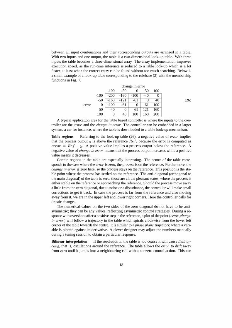
between all input combinations and their corresponding outputs are arranged in a table.With two inputs and one output, the table is a two-dimensional look-up table. With threeinputs the table becomes a three-dimensional array. The array implementation improvesexecution speed, as the run-time inference is reduced to a table look-up which is a lotfaster, at least when the correct entry can be found without too much searching. Below isa small example of a look-up table corresponding to the rulebase (2) with the membershipfunctions in Fig. 7,

change in error-100 -50 0 50 100

-100 -200 -160 -100 -40 0-50 -160 -121 -61 0 40

error 0 -100 -61 0 61 10050 -40 0 61 121 160

100 0 40 100 160 200

(26)

A typical application area for the table based controller is where the inputs to the con-troller are the HUURU and the FKDQJH LQ HUURU. The controller can be embedded in a largersystem, a car for instance, where the table is downloaded to a table look-up mechanism.

7DEOH UHJLRQV Referring to the look-up table (26), a negative value of HUURU impliesthat the process output | is above the reference Uhi , because the error is computed ashuuru @ Uhi � |. A positive value implies a process output below the reference. Anegative value of FKDQJH LQ HUURU means that the process output increases while a positivevalue means it decreases.

Certain regions in the table are especially interesting. The centre of the table corre-sponds to the case where the HUURU is zero, the process is on the reference. Furthermore, theFKDQJH LQ HUURU is zero here, so the process stays on the reference. This position is the sta-ble point where the process has settled on the reference. The anti-diagonal (orthogonal tothe main diagonal) of the table is zero; those are all the pleasant states, where the process iseither stable on the reference or approaching the reference. Should the process move awaya little from the zero diagonal, due to noise or a disturbance, the controller will make smallcorrections to get it back. In case the process is far from the reference and also movingaway from it, we are in the upper left and lower right corners. Here the controller calls fordrastic changes.

The numerical values on the two sides of the zero diagonal do not have to be anti-symmetric; they can be any values, reflecting asymmetric control strategies. During a re-sponse with overshoot after a positive step in the reference, a plot of the point +HUURU >FKDQJHLQ HUURU , will follow a trajectory in the table which spirals clockwise from the lower leftcorner of the table towards the centre. It is similar to a SKDVH SODQH trajectory, where a vari-able is plotted against its derivative. A clever designer may adjust the numbers manuallyduring a tuning session to obtain a particular response.

%LOLQHDU LQWHUSRODWLRQ If the resolution in the table is too coarse it will cause OLPLW F\�FOLQJ, that is, oscillations around the reference. The table allows the HUURU to drift awayfrom zero until it jumps into a neighbouring cell with a nonzero control action. This can

18

be avoided with ELOLQHDU LQWHUSRODWLRQ between the cells instead of rounding to the nearestpoint. In the case of a two-dimensional table, an error H satisfies the relation H4 � H �H5, where H4 and H5 are the two neighbouring points. The change-in-error FH will like-wise satisfy FH4 � FH � FH5. The resulting table value is then found by interpolatinglinearly in the H axis direction between the first pair x4 @ +I +H4> FH4,> I +H5> FH4,,and the second pair x5 @ +I +H4> FH5,> I +H5> FH5,,, and then in the FH-axis directionbetween the pair +x4> x5,.

q�'LPHQVLRQDO 7DEOHV A three input controller has a three-dimensional look-up table.Assuming a resolution of, say, 13 points in each universe, the table holds 2197 elements. Itwould be a tremendous task to fill these in manually, but it is manageable with rules.

A three dimensional table can be represented as a two-dimensional table using a re-lational representation. Rearrange the table into three columns one for each of the threeinputs +H4> H5> H6, and one for the output +X, > for example Table 1. Each input can takefive values, and the table thus has 8 � 8 � 8 @ 458 rows. The table look-up is now aquestion of finding the right row, and picking the corresponding X value.

H4 H5 H6 X�433 �433 �433 �433�433 �433 �9: �;<�433 �433 3 �9:�433 �433 9: �4:;�433 �433 433 �66�433 �9: �433 �;<�433 �9: �9: �4;<�433 �9: 3 �89

� � � � � � � � � � � �433 433 433 433

Table 1: Equivalent of a 3D look-up table.

�� ,QSXW�2XWSXW 0DSSLQJ

Two inputs and one output results in a two dimensional table, which can be plotted as asurface for visual inspection. The relationship between one input and one output can beplotted as a graph. These plots are a design aid when selecting membership functions andconstructing rules.

The shape of the surface can be controlled to a certain extent by manipulating the mem-bership functions. In order to see this clearly, we will use the one-input-one-output case(without loss of generality). The fuzzy proportional rule base

1. If error is Neg then output is Neg

2. If error is Zero then output is Zero (27)

19

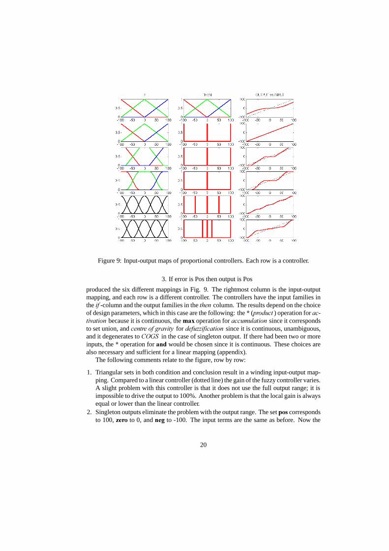
Figure 9: Input-output maps of proportional controllers. Each row is a controller.

3. If error is Pos then output is Pos

produced the six different mappings in Fig. 9. The rightmost column is the input-outputmapping, and each row is a different controller. The controllers have the input families inthe LI -column and the output families in the WKHQ column. The results depend on the choiceof design parameters, which in this case are the following: the (SURGXFW ) operation for DF�WLYDWLRQ because it is continuous, the PD[ operation for DFFXPXODWLRQ since it correspondsto set union, and FHQWUH RI JUDYLW\ for GHIX]]LILFDWLRQ since it is continuous, unambiguous,and it degenerates to &2*6 in the case of singleton output. If there had been two or moreinputs, the operation for DQG would be chosen since it is continuous. These choices arealso necessary and sufficient for a linear mapping (appendix).

The following comments relate to the figure, row by row:

1. Triangular sets in both condition and conclusion result in a winding input-output map-ping. Compared to a linear controller (dotted line) the gain of the fuzzy controller varies.A slight problem with this controller is that it does not use the full output range; it isimpossible to drive the output to 100%. Another problem is that the local gain is alwaysequal or lower than the linear controller.

2. Singleton outputs eliminate the problem with the output range. The set SRV correspondsto 100, ]HUR to 0, and QHJ to -100. The input terms are the same as before. Now the

20

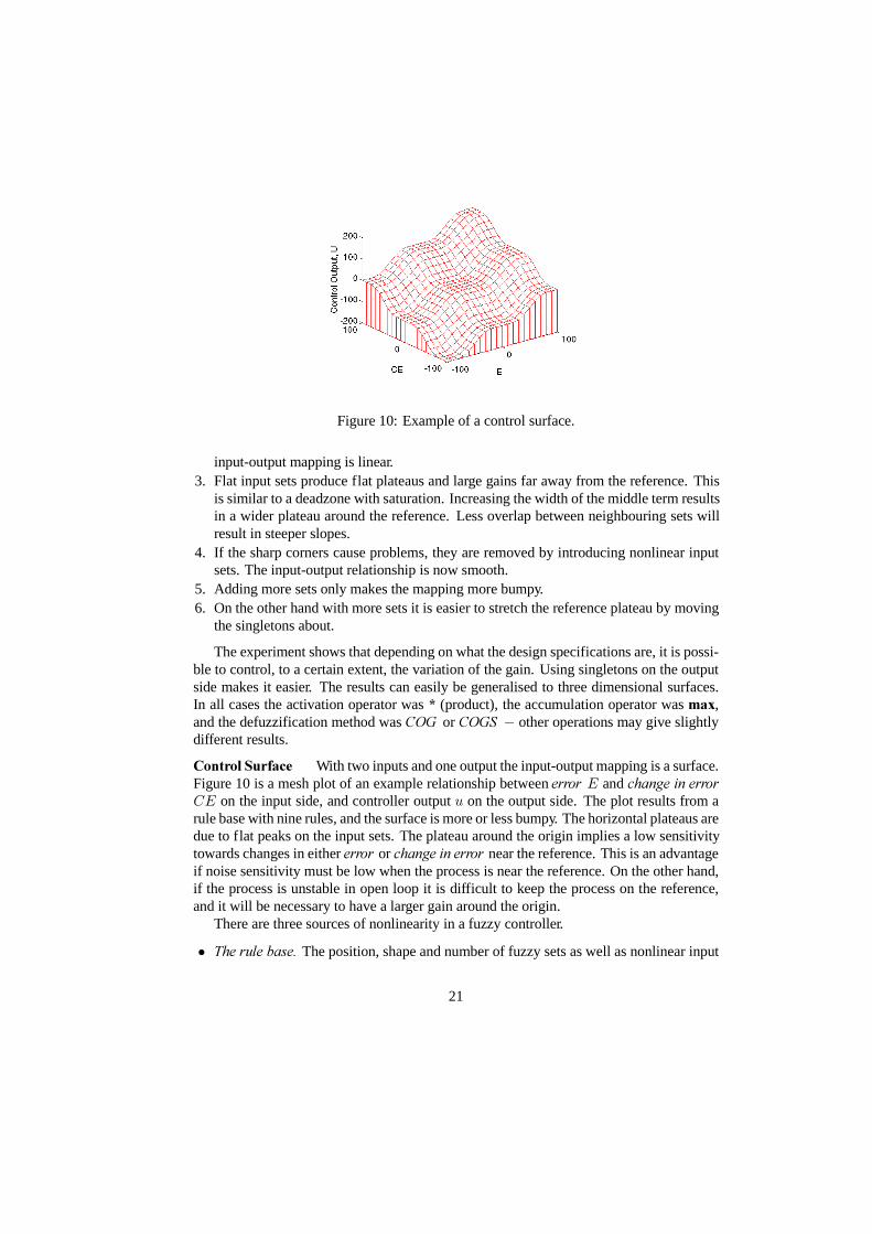
Figure 10: Example of a control surface.

input-output mapping is linear.3. Flat input sets produce flat plateaus and large gains far away from the reference. This

is similar to a deadzone with saturation. Increasing the width of the middle term resultsin a wider plateau around the reference. Less overlap between neighbouring sets willresult in steeper slopes.

4. If the sharp corners cause problems, they are removed by introducing nonlinear inputsets. The input-output relationship is now smooth.

5. Adding more sets only makes the mapping more bumpy.6. On the other hand with more sets it is easier to stretch the reference plateau by moving

the singletons about.

The experiment shows that depending on what the design specifications are, it is possi-ble to control, to a certain extent, the variation of the gain. Using singletons on the outputside makes it easier. The results can easily be generalised to three dimensional surfaces.In all cases the activation operator was (product), the accumulation operator was PD[,and the defuzzification method was &2* or &2*6 � other operations may give slightlydifferent results.

&RQWURO 6XUIDFH With two inputs and one output the input-output mapping is a surface.Figure 10 is a mesh plot of an example relationship between HUURU H and FKDQJH LQ HUURUFH on the input side, and controller output x on the output side. The plot results from arule base with nine rules, and the surface is more or less bumpy. The horizontal plateaus aredue to flat peaks on the input sets. The plateau around the origin implies a low sensitivitytowards changes in either HUURU or FKDQJH LQ HUURU near the reference. This is an advantageif noise sensitivity must be low when the process is near the reference. On the other hand,if the process is unstable in open loop it is difficult to keep the process on the reference,and it will be necessary to have a larger gain around the origin.

There are three sources of nonlinearity in a fuzzy controller.

� 7KH UXOH EDVH� The position, shape and number of fuzzy sets as well as nonlinear input

21

scaling cause nonlinear transformations. The rules often express a nonlinear controlstrategy.

� 7KH LQIHUHQFH HQJLQH� If the connectives DQG and RU are implemented as for examplePLQ and PD[ respectively, they are nonlinear.

� 7KH GHIX]]LILFDWLRQ. Several defuzzification methods are nonlinear.

It is possible to construct a rule base with a linear input-output mapping (Siler & Ying,1989; Mizumoto, 1992; Qiao & Mizumoto; 1996). The following checklist summarises thegeneral design choices for achieving a fuzzy rule base equivalent to a summation (detailsin the appendix):

� Use triangular input sets that cross at � @ 3=8>

� use the algebraic product (*) for the DQG connective;� the rule base must be the complete DQG combination (cartesian product) of all input

families;� use output singletons, positions determined by the sum of the peak positions of the input

sets;� use &2*6 defuzzification.

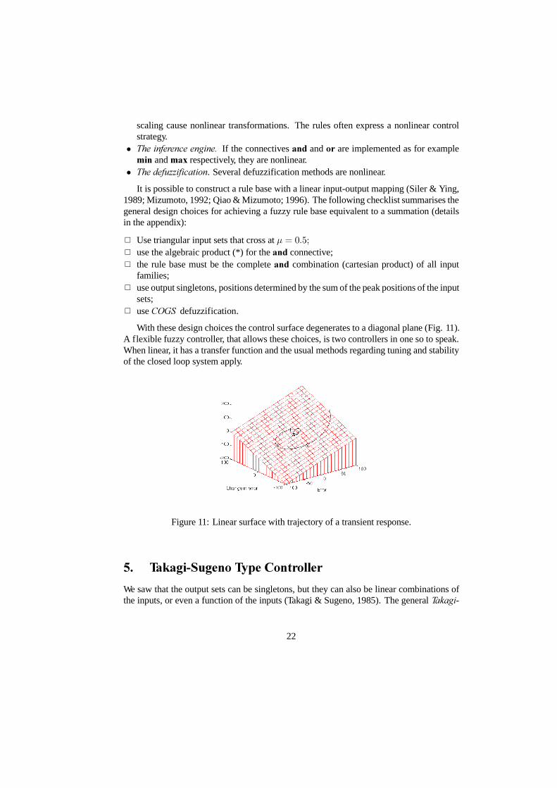
With these design choices the control surface degenerates to a diagonal plane (Fig. 11).A flexible fuzzy controller, that allows these choices, is two controllers in one so to speak.When linear, it has a transfer function and the usual methods regarding tuning and stabilityof the closed loop system apply.

Figure 11: Linear surface with trajectory of a transient response.

�� 7DNDJL�6XJHQR 7\SH &RQWUROOHU

We saw that the output sets can be singletons, but they can also be linear combinations ofthe inputs, or even a function of the inputs (Takagi & Sugeno, 1985). The general 7DNDJL�

22

0 50 1000

50

100

150

(a)

outp

ut

1

2

0 50 1000

0.5

1

(b)

mem

bers

hip

Figure 12: Interpolation between two lines (a), and overlap of rules (b).

6XJHQR rule structure is

If i+h4 is $4> h5 is $5> = = = > hn is $n, then | @ j+h4> h4 = = =,

Here i is a logical function that connects the sentences forming the condition, | is theoutput, and j is a function of the inputs. A simple example is

If error is Zero and change in error is Zero then output | @ f

where f is a crisp constant. This is a ]HUR�RUGHU model, and it is identical to singleton outputrules. A slightly more complex rule is

If error is Zero and change in error is Zero then output

| @ d � huuru . e � +fkdqjh lq huuru, . f

where d> e and f are all constants. This is a ILUVW�RUGHU model. Inference with severalrules proceeds as usual, with a firing strength associated with each rule, but each outputis linearly dependent on the inputs. The output from each rule is a moving singleton, andthe defuzzified output is the weighted average of the contributions from each rule. Thecontroller interpolates between linear controllers; each controller is dominated by a rule,but there is a weighting depending on the overlap of the input membership functions. Thisis useful in a nonlinear control system, where each controller operates in a subspace ofthe operating envelope. One can say that the rules interpolate smoothly between the lineargains. Higher order models are also possible.

([DPSOH � �6XJHQR� 6XSSRVH ZH KDYH WZR UXOHV

�� ,I HUURU LV /DUJH WKHQ RXWSXW LV /LQH�

�� ,I HUURU LV 6PDOO WKHQ RXWSXW LV /LQH�

/LQH � LV GHILQHG DV 3=5�huuru.<3 DQG OLQH � LV GHILQHG DV 3=9�huuru.53� 7KH UXOHV

23

LQWHUSRODWH EHWZHHQ WKH WZR OLQHV LQ WKH UHJLRQ ZKHUH WKH PHPEHUVKLS IXQFWLRQV RYHUODS�)LJ� 12�� 2XWVLGH RI WKDW UHJLRQ WKH RXWSXW LV D OLQHDU IXQFWLRQ RI WKH huuru� 7KLV W\SH RIPRGHO LV XVHG LQ QHXURIX]]\ V\VWHPV�

In order to train a model to incorporate dynamics of a target system, the input is aug-mented with signals corresponding to past inputs x and outputs |. In the time discretedomain the output of the model |p> with superscript p referring to the model and s to theplant, is

|p+w. 4, @ ei ^|s+w,> = = = > |s+w� q. 4,>x+w,> = = = > x+w�p. 4,` (28)

Here ei represents the nonlinear input-output map of the model (i.e. the approximation ofthe target system i). Notice that the input to the model includes the past values of the plantoutput |s and the plant input x.

�� 6XPPDU\

In a fuzzy controller the data passes through a preprocessing block, a controller, and apostprocessing block. Preprocessing consists of a linear or non-linear scaling as well as aquantisation in case the membership functions are discretised (vectors); if not, the mem-bership of the input can just be looked up in an appropriate function. When designing therule base, the designer needs to consider the number of term sets, their shape, and theiroverlap. The rules themselves must be determined by the designer, unless more advancedmeans like self-organisation or neural networks are available. There is a choice betweenmultiplication and minimum in the activation. There is also a choice regarding defuzzifi-cation; FHQWUH RI JUDYLW\ is probably most widely used. The postprocessing consists in ascaling of the output. In case the controller is incremental, postprocessing also includes anintegration. The following is a checklist of design choices that have to be made:

� 5XOH EDVH UHODWHG FKRLFHV. Number of inputs and outputs, rules, universes, continuous@ discrete, the number of membership functions, their overlap and width, singletonoutput;

� ,QIHUHQFH HQJLQH UHODWHG FKRLFHV. Connectives, modifiers, activation operation, aggre-gation operation, and accumulation operation.

� 'HIX]]LILFDWLRQ PHWKRG. COG, COGS, BOA, MOM, LM, and RM.� 3UH� DQG SRVW�SURFHVVLQJ. Scaling, gain factors, quantisation, and sampling time.

Some of these items must always be considered, others may not play a role in the par-ticular design.

The input-output mappings provide an intuitive insight which may not be relevant froma theoretical viewpoint, but in practice they are well worth using. The analysis representedby plots is limited, though, to three dimensions. Various input-output mappings can beobtained by changing the fuzzy membership functions, and the chapter shows how to obtaina linear mapping with only a few adjustments.

The linear fuzzy controller may be used in a design procedure based on PID control:

24

1. Tune a PID controller.2. Replace it with a linear fuzzy controller.3. Transfer gains.4. Make the fuzzy controller nonlinear.5. Fine-tune it.

It seems sensible to start the controller design with a crisp PID controller, maybe evenjust a P controller, and get the system stabilised. From there it is easier to go to fuzzycontrol.

5HIHUHQFHV

Driankov, D., Hellendoorn, H. and Reinfrank, M. (1996). $Q LQWURGXFWLRQ WR IX]]\ FRQWURO, secondedn, Springer-Verlag, Berlin.

Hill, G., Horstkotte, E. and Teichrow, J. (1990). )X]]\�& GHYHORSPHQW V\VWHP ± XVHU�V PDQXDO,Togai Infralogic, 30 Corporate Park, Irvine, CA 92714, USA.

Holmblad, L. P. and Østergaard, J.-J. (1982). Control of a cement kiln by fuzzy logic,LQ Guptaand Sanchez (eds),)X]]\ ,QIRUPDWLRQ DQG'HFLVLRQ 3URFHVVHV, North-Holland, Amsterdam,pp. 389–399. (Reprint in: FLS Review No 67, FLS Automation A/S, Høffdingsvej 77, DK-2500 Valby, Copenhagen, Denmark).

IEC (1996). Programmable controllers: Part 7 fuzzy control programming,7HFKQLFDO 5HSRUW,(& ����, International Electrotechnical Commission. (Draft.).

Lee, C. C. (1990). Fuzzy logic in control systems: Fuzzy logic controller,,((( 7UDQV� 6\VWHPV�0DQ &\EHUQHWLFV ��(2): 404–435.

MIT (1995). &,7( /LWHUDWXUH DQG 3URGXFWV 'DWDEDVH, MIT GmbH / ELITE, Promenade 9, D-52076 Aachen, Germany.

Mizumoto, M. (1992). Realization of PID controls by fuzzy control methods,LQ IEEE (ed.),)LUVW ,QW� &RQI� 2Q )X]]\ 6\VWHPV, number 92CH3073-4, The Institute of Electrical andElectronics Engineers, Inc, San Diego, pp. 709–715.

Passino, K. M. and Yurkovich, S. (1998).)X]]\ &RQWURO, Addison Wesley Longman, Inc, MenloPark, CA, USA.

Pedrycz, W. (1993).)X]]\ FRQWURO DQG IX]]\ V\VWHPV, second edn, Wiley and Sons, New York.Qiao, W. and Mizumoto, M. (1996). PID type fuzzy controller and parameters adaptive method,

)X]]\ 6HWV DQG 6\VWHPV ��: 23–35.Siler, W. and Ying, H. (1989). Fuzzy control theory: The linear case,)X]]\ 6HWV DQG 6\VWHPV

��: 275–290.Takagi, T. and Sugeno, M. (1985). Fuzzy identification of systems and its applications to mod-

eling and control,,((( 7UDQV� 6\VWHPV� 0DQ &\EHUQHWLFV ��(1): 116–132.

25

$SSHQGL[ $� $GGLWLYH 5XOH %DVH

The input universes must be large enough for the inputs to stay within the limits (no VDWX�UDWLRQ ). Each input family should contain a number of terms, designed such that the sumof membership values for each input is 1. This can be achieved when the sets are triangularand cross their neighbour sets at the membership value � @ 3=8> their peaks will thus beequidistant. Any input value can thus be a member of at most two sets, and the membershipof each is a linear function of the input value. Take for example the rule base

1. If H is Pos and FH is Pos then x is v4 (A-1)

2. If H is Pos and FH is Neg then x is v53. If H is Neg and FH is Pos then x is v64. If H is Neg and FH is Neg then x is v7

Assume both inputs, H and FH> are defined on a standard universe ^�433> 433` > that Posis a triangle with its peak at 100 and left base vertex in -100, and that Neg is a triangle withits peak at -100 and right base vertex in 100. For the first rule in (A-1) the membership ofa given input value of H in Pos is �Srv+H,= The aggregation �4 of the first rule is

�4 @ �Srv+H, a �Srv+FH, (A-2)

where the symbol a denotes the fuzzy DQG operation.The number of terms in each family determines the number of rules, as they must be theDQG combination (RXWHU SURGXFW ) of all terms to ensure completeness. The output setsshould preferably be singletons vl equal to the sum of the peak positions of the input sets.The output sets may also be triangles, symmetric about their peaks, but singletons makedefuzzification simpler.To ensure linearity, we must choose the algebraic product for the connective DQG. Usingthe weighted average of rule contributions for the control signal (corresponding to FHQWUH RIJUDYLW\ defuzzification, &2* ), the denominator does not affect the calculations, becauseall firing strengths add up to 1.What has been said can be generalised to input families with more than two input sets perinput, because only two input sets will be active at a time.3URRI� $GGLWLYH UXOH EDVH. Returning to the rule base (A-1), the contribution to the controlsignal from the first rule is

�4� v4 @ �Srv+H, a �Srv+FH, � v4 (A-3)

@ �Srv+H, � �Srv+FH, � v4 (A-4)

The combination of all contributions, using &2* defuzzification is

x @�4 � v4 . �5 � v5 . �6 � v6 . �7 � v7

�4 . �5 . �6 . �7(A-5)

To keep the notation simple we will substitute

{ @ �Srv+H, (A-6)

| @ �Srv+FH, (A-7)

4� { @ �Qhj+H, (A-8)

26

4� | @ �Qhj+FH, (A-9)

Observe that if we add the terms from rule 1 and rule 3 in the denominator of (A-5), we get

�4. �

6@ {| . +4� {, | (A-10)

@ | (A-11)

This is because of the special setup of the triangular membership functions. Similarly weget

�5 . �7 @ 4� | (A-12)Therefore

�4. �

6. �

5. �

7@ 4 (A-13)

That explains why the denominator in (A-5) vanishes. Its numerator Q+H>FH, is a dif-ferent story,

Q+H>FH, @ �4� v4 . �

5� v5 . �

6� v6 . �

7� v7 (A-14)

@ {|v4 . { +4� |, v5 . +4� {, |v6 . +4� {, +4� |, v7 (A-15)

Clearly {> | 5 ^3> 4` since they are really fuzzy membership functions, and (A-15) is simplya bilinear interpolation between the four scalars v4> = = = > v7. Since { is a linear function inH and | is a linear function in FH, the numerator Q+H>FH,, and thereby the controlleroutput Xq, is a bilinear function in H and FH. When +{> |, @ +4> 4, all other terms but theone holding v4 are zero, and when +{> |, @ +4> 3, all other terms but the one holding v5 arezero, etc. Since +{> |, @ +4> 4, when +H>FH, @ +433> 433, > then v4 should be chosen tobe 533 in order to obtain the sought equivalence with the summation H .FH. The rest ofthe singletons should be chosen in a similar way, yielding

+v4> v5> v6> v7, @ +533> 3> 3>�533,

27