Neural Fuzzy Systems - Petra Christian...
253
Neural Fuzzy Systems Robert Full´ er Donner Visiting professor ˚ Abo Akademi University ISBN 951-650-624-0, ISSN 0358-5654 ˚ Abo 1995
-
Upload
hoangnguyet -
Category
Documents
-
view
217 -
download
1
Transcript of Neural Fuzzy Systems - Petra Christian...
Neural Fuzzy Systems
Robert Fuller
Donner Visiting professor
Abo Akademi University
ISBN 951-650-624-0, ISSN 0358-5654
Abo 1995
Contents
0.1 Preface . . . . . . . . . . . . . . . . . . . . . . . . . . . . . . . . . . . . . . 3
1 Fuzzy Systems 8
1.1 An introduction to fuzzy logic . . . . . . . . . . . . . . . . . . . . . . . . . 8
1.2 Operations on fuzzy sets . . . . . . . . . . . . . . . . . . . . . . . . . . . . 18
1.3 Fuzzy relations . . . . . . . . . . . . . . . . . . . . . . . . . . . . . . . . . 24
1.3.1 The extension principle . . . . . . . . . . . . . . . . . . . . . . . . . 32
1.3.2 Metrics for fuzzy numbers . . . . . . . . . . . . . . . . . . . . . . . 42
1.3.3 Fuzzy implications . . . . . . . . . . . . . . . . . . . . . . . . . . . 44
1.3.4 Linguistic variables . . . . . . . . . . . . . . . . . . . . . . . . . . . 48
1.4 The theory of approximate reasoning . . . . . . . . . . . . . . . . . . . . . 50
1.5 An introduction to fuzzy logic controllers . . . . . . . . . . . . . . . . . . . 66
1.5.1 Defuzzification methods . . . . . . . . . . . . . . . . . . . . . . . . 72
1.5.2 Inference mechanisms . . . . . . . . . . . . . . . . . . . . . . . . . . 75
1.5.3 Construction of data base and rule base of FLC . . . . . . . . . . . 80
1.5.4 Ball and beam problem . . . . . . . . . . . . . . . . . . . . . . . . . 85
1.6 Aggregation in fuzzy system modeling . . . . . . . . . . . . . . . . . . . . 88
1.6.1 Averaging operators . . . . . . . . . . . . . . . . . . . . . . . . . . 91
1.7 Fuzzy screening systems . . . . . . . . . . . . . . . . . . . . . . . . . . . . 100
1.8 Applications of fuzzy systems . . . . . . . . . . . . . . . . . . . . . . . . . 106
2 Artificial Neural Networks 118
2.1 The perceptron learning rule . . . . . . . . . . . . . . . . . . . . . . . . . . 118
2.2 The delta learning rule . . . . . . . . . . . . . . . . . . . . . . . . . . . . . 128
2.2.1 The delta learning rule with semilinear activation function . . . . . 134
2.3 The generalized delta learning rule . . . . . . . . . . . . . . . . . . . . . . 138
2.3.1 Effectivity of neural networks . . . . . . . . . . . . . . . . . . . . . 141
2.4 Winner-take-all learning . . . . . . . . . . . . . . . . . . . . . . . . . . . . 143
2.5 Applications of artificial neural networks . . . . . . . . . . . . . . . . . . . 147
3 Fuzzy Neural Networks 153
3.1 Integration of fuzzy logic and neural networks . . . . . . . . . . . . . . . . 153
1

3.1.1 Fuzzy neurons . . . . . . . . . . . . . . . . . . . . . . . . . . . . . . 157
3.2 Hybrid neural nets . . . . . . . . . . . . . . . . . . . . . . . . . . . . . . . 165
3.2.1 Computation of fuzzy logic inferences by hybrid neural net . . . . . 174
3.3 Trainable neural nets for fuzzy IF-THEN rules . . . . . . . . . . . . . . . . 180
3.3.1 Implementation of fuzzy rules by regular FNN of Type 2 . . . . . . 187
3.3.2 Implementation of fuzzy rules by regular FNN of Type 3 . . . . . . 190
3.4 Tuning fuzzy control parameters by neural nets . . . . . . . . . . . . . . . 194
3.5 Fuzzy rule extraction from numerical data . . . . . . . . . . . . . . . . . . 201
3.6 Neuro-fuzzy classifiers . . . . . . . . . . . . . . . . . . . . . . . . . . . . . 204
3.7 FULLINS . . . . . . . . . . . . . . . . . . . . . . . . . . . . . . . . . . . . 210
3.8 Applications of fuzzy neural systems . . . . . . . . . . . . . . . . . . . . . 215
4 Appendix 230
4.1 Case study: A portfolio problem . . . . . . . . . . . . . . . . . . . . . . . . 230
4.2 Exercises . . . . . . . . . . . . . . . . . . . . . . . . . . . . . . . . . . . . . 234
2
0.1 Preface
This Lecture Notes containes the material of the course on Neural Fuzzy Systems deliveredby the author at Turku Center for Computer Science in 1995.
Fuzzy sets were introduced by Zadeh (1965) as a means of representing and manipulatingdata that was not precise, but rather fuzzy. Fuzzy logic provides an inference morphologythat enables approximate human reasoning capabilities to be applied to knowledge-basedsystems. The theory of fuzzy logic provides a mathematical strength to capture the uncer-tainties associated with human cognitive processes, such as thinking and reasoning. Theconventional approaches to knowledge representation lack the means for representatingthe meaning of fuzzy concepts. As a consequence, the approaches based on first orderlogic and classical probablity theory do not provide an appropriate conceptual frameworkfor dealing with the representation of commonsense knowledge, since such knowledge isby its nature both lexically imprecise and noncategorical.
The developement of fuzzy logic was motivated in large measure by the need for a con-ceptual framework which can address the issue of uncertainty and lexical imprecision.
Some of the essential characteristics of fuzzy logic relate to the following [120].
• In fuzzy logic, exact reasoning is viewed as a limiting case of approximatereasoning.
• In fuzzy logic, everything is a matter of degree.
• In fuzzy logic, knowledge is interpreted a collection of elastic or, equiva-lently, fuzzy constraint on a collection of variables.
• Inference is viewed as a process of propagation of elastic constraints.
• Any logical system can be fuzzified.
There are two main characteristics of fuzzy systems that give them better performancefor specific applications.
• Fuzzy systems are suitable for uncertain or approximate reasoning, especially forthe system with a mathematical model that is difficult to derive.
• Fuzzy logic allows decision making with estimated values under incomplete or un-certain information.
Artificial neural systems can be considered as simplified mathematical models of brain-like systems and they function as parallel distributed computing networks. However,in contrast to conventional computers, which are programmed to perform specific task,most neural networks must be taught, or trained. They can learn new associations, newfunctional dependencies and new patterns.
The study of brain-style computation has its roots over 50 years ago in the work of Mc-Culloch and Pitts (1943) and slightly later in Hebb’s famous Organization of Behavior(1949). The early work in artificial intelligence was torn between those who believed thatintelligent systems could best be built on computers modeled after brains, and those likeMinsky and Papert who believed that intelligence was fundamentally symbol processing
3
of the kind readily modeled on the von Neumann computer. For a variety of reasons,the symbol-processing approach became the dominant theme in artifcial intelligence. The1980s showed a rebirth in interest in neural computing: Hopfield (1985) provided themathematical foundation for understanding the dynamics of an important class of net-works; Rumelhart and McClelland (1986) introduced the backpropagation learning algo-rithm for complex, multi-layer networks and thereby provided an answer to one of themost severe criticisms of the original perceptron work.
Perhaps the most important advantage of neural networks is their adaptivity. Neuralnetworks can automatically adjust their weights to optimize their behavior as patternrecognizers, decision makers, system controllers, predictors, etc. Adaptivity allows theneural network to perform well even when the environment or the system being con-trolled varies over time. There are many control problems that can benefit from continualnonlinear modeling and adaptation.
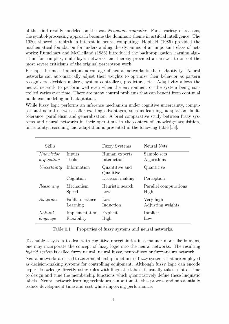
While fuzzy logic performs an inference mechanism under cognitive uncertainty, compu-tational neural networks offer exciting advantages, such as learning, adaptation, fault-tolerance, parallelism and generalization. A brief comparative study between fuzzy sys-tems and neural networks in their operations in the context of knowledge acquisition,uncertainty, reasoning and adaptation is presented in the following table [58]:
Skills Fuzzy Systems Neural Nets
Knowledge Inputs Human experts Sample setsacquisition Tools Interaction Algorithms
Uncertainty Information Quantitive and QuantitiveQualitive
Cognition Decision making Perception
Reasoning Mechanism Heuristic search Parallel computationsSpeed Low High
Adaption Fault-tolerance Low Very highLearning Induction Adjusting weights
Natural Implementation Explicit Implicitlanguage Flexibility High Low
Table 0.1 Properties of fuzzy systems and neural networks.
To enable a system to deal with cognitive uncertainties in a manner more like humans,one may incorporate the concept of fuzzy logic into the neural networks. The resultinghybrid system is called fuzzy neural, neural fuzzy, neuro-fuzzy or fuzzy-neuro network.
Neural networks are used to tune membership functions of fuzzy systems that are employedas decision-making systems for controlling equipment. Although fuzzy logic can encodeexpert knowledge directly using rules with linguistic labels, it usually takes a lot of timeto design and tune the membership functions which quantitatively define these linquisticlabels. Neural network learning techniques can automate this process and substantiallyreduce development time and cost while improving performance.
4
x1
xn
w1
wn
y = f(<w, x>) f
In theory, neural networks, and fuzzy systems are equivalent in that they are convertible,yet in practice each has its own advantages and disadvantages. For neural networks, theknowledge is automatically acquired by the backpropagation algorithm, but the learningprocess is relatively slow and analysis of the trained network is difficult (black box).Neither is it possible to extract structural knowledge (rules) from the trained neuralnetwork, nor can we integrate special information about the problem into the neuralnetwork in order to simplify the learning procedure.
Fuzzy systems are more favorable in that their behavior can be explained based on fuzzyrules and thus their performance can be adjusted by tuning the rules. But since, in general,knowledge acquisition is difficult and also the universe of discourse of each input variableneeds to be divided into several intervals, applications of fuzzy systems are restricted tothe fields where expert knowledge is available and the number of input variables is small.
To overcome the problem of knowledge acquisition, neural networks are extended to au-tomatically extract fuzzy rules from numerical data.
Cooperative approaches use neural networks to optimize certain parameters of an ordinaryfuzzy system, or to preprocess data and extract fuzzy (control) rules from data.
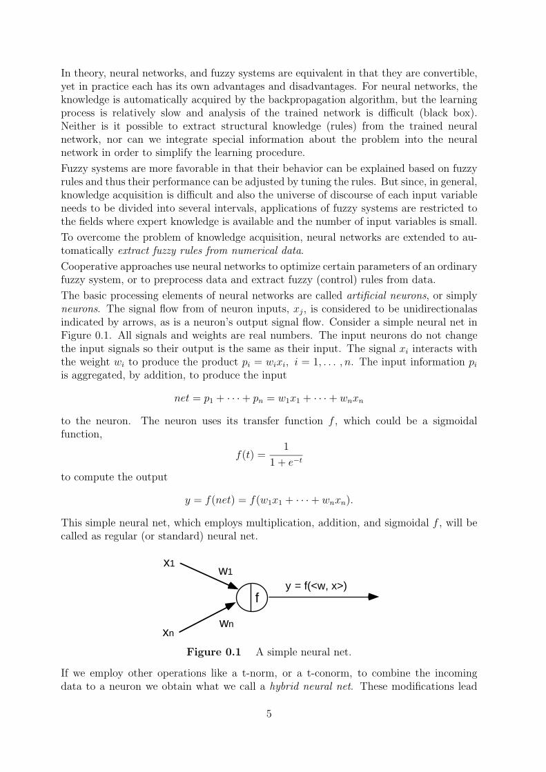
The basic processing elements of neural networks are called artificial neurons, or simplyneurons. The signal flow from of neuron inputs, xj, is considered to be unidirectionalasindicated by arrows, as is a neuron’s output signal flow. Consider a simple neural net inFigure 0.1. All signals and weights are real numbers. The input neurons do not changethe input signals so their output is the same as their input. The signal xi interacts withthe weight wi to produce the product pi = wixi, i = 1, . . . , n. The input information piis aggregated, by addition, to produce the input
net = p1 + · · ·+ pn = w1x1 + · · ·+ wnxn
to the neuron. The neuron uses its transfer function f , which could be a sigmoidalfunction,
f(t) =1
1 + e−t
to compute the output
y = f(net) = f(w1x1 + · · ·+ wnxn).
This simple neural net, which employs multiplication, addition, and sigmoidal f , will becalled as regular (or standard) neural net.
Figure 0.1 A simple neural net.
If we employ other operations like a t-norm, or a t-conorm, to combine the incomingdata to a neuron we obtain what we call a hybrid neural net. These modifications lead
5
to a fuzzy neural architecture based on fuzzy arithmetic operations. A hybrid neural netmay not use multiplication, addition, or a sigmoidal function (because the results of theseoperations are not necesserily are in the unit interval).
A hybrid neural net is a neural net with crisp signals and weights and crisp transferfunction. However, (i) we can combine xi and wi using a t-norm, t-conorm, or some othercontinuous operation; (ii) we can aggregate the pi’s with a t-norm, t-conorm, or any othercontinuous function; (iii) f can be any continuous function from input to output.
We emphasize here that all inputs, outputs and the weights of a hybrid neural net arereal numbers taken from the unit interval [0, 1]. A processing element of a hybrid neuralnet is called fuzzy neuron.
It is well-known that regular nets are universal approximators, i.e. they can approximateany continuous function on a compact set to arbitrary accuracy. In a discrete fuzzyexpert system one inputs a discrete approximation to the fuzzy sets and obtains a discreteapproximation to the output fuzzy set. Usually discrete fuzzy expert systems and fuzzycontrollers are continuous mappings. Thus we can conclude that given a continuous fuzzyexpert system, or continuous fuzzy controller, there is a regular net that can uniformlyapproximate it to any degree of accuracy on compact sets. The problem with this resultthat it is non-constructive and does not tell you how to build the net.
Hybrid neural nets can be used to implement fuzzy IF-THEN rules in a constructive way.Though hybrid neural nets can not use directly the standard error backpropagation algo-rithm for learning, they can be trained by steepest descent methods to learn the parametersof the membership functions representing the linguistic terms in the rules.
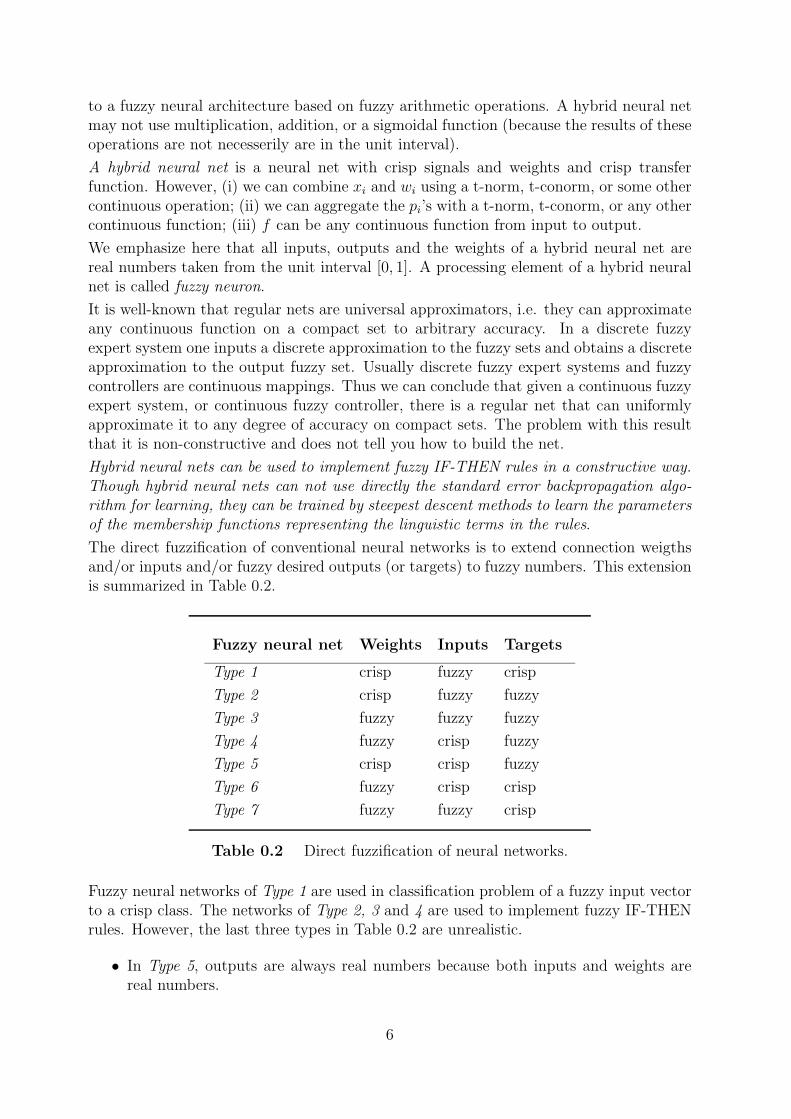
The direct fuzzification of conventional neural networks is to extend connection weigthsand/or inputs and/or fuzzy desired outputs (or targets) to fuzzy numbers. This extensionis summarized in Table 0.2.
Fuzzy neural net Weights Inputs Targets
Type 1 crisp fuzzy crisp
Type 2 crisp fuzzy fuzzy
Type 3 fuzzy fuzzy fuzzy
Type 4 fuzzy crisp fuzzy
Type 5 crisp crisp fuzzy
Type 6 fuzzy crisp crisp
Type 7 fuzzy fuzzy crisp
Table 0.2 Direct fuzzification of neural networks.
Fuzzy neural networks of Type 1 are used in classification problem of a fuzzy input vectorto a crisp class. The networks of Type 2, 3 and 4 are used to implement fuzzy IF-THENrules. However, the last three types in Table 0.2 are unrealistic.
• In Type 5, outputs are always real numbers because both inputs and weights arereal numbers.
6
X1
Xn
W1
Wn
Y = f(W1X1+ ... + WnXn)
• In Type 6 and 7, the fuzzification of weights is not necessary because targets arereal numbers.
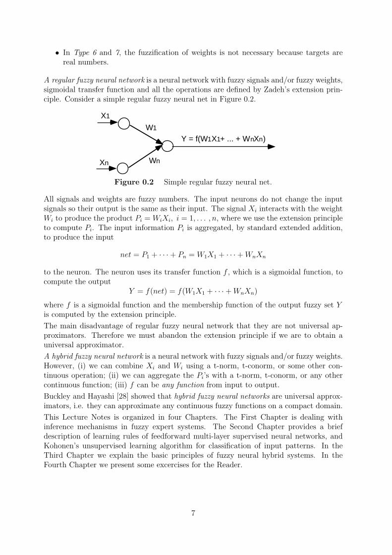
A regular fuzzy neural network is a neural network with fuzzy signals and/or fuzzy weights,sigmoidal transfer function and all the operations are defined by Zadeh’s extension prin-ciple. Consider a simple regular fuzzy neural net in Figure 0.2.
Figure 0.2 Simple regular fuzzy neural net.
All signals and weights are fuzzy numbers. The input neurons do not change the inputsignals so their output is the same as their input. The signal Xi interacts with the weightWi to produce the product Pi = WiXi, i = 1, . . . , n, where we use the extension principleto compute Pi. The input information Pi is aggregated, by standard extended addition,to produce the input
net = P1 + · · ·+ Pn = W1X1 + · · ·+WnXn
to the neuron. The neuron uses its transfer function f , which is a sigmoidal function, tocompute the output
Y = f(net) = f(W1X1 + · · ·+WnXn)
where f is a sigmoidal function and the membership function of the output fuzzy set Yis computed by the extension principle.
The main disadvantage of regular fuzzy neural network that they are not universal ap-proximators. Therefore we must abandon the extension principle if we are to obtain auniversal approximator.
A hybrid fuzzy neural network is a neural network with fuzzy signals and/or fuzzy weights.However, (i) we can combine Xi and Wi using a t-norm, t-conorm, or some other con-tinuous operation; (ii) we can aggregate the Pi’s with a t-norm, t-conorm, or any othercontinuous function; (iii) f can be any function from input to output.
Buckley and Hayashi [28] showed that hybrid fuzzy neural networks are universal approx-imators, i.e. they can approximate any continuous fuzzy functions on a compact domain.
This Lecture Notes is organized in four Chapters. The First Chapter is dealing withinference mechanisms in fuzzy expert systems. The Second Chapter provides a briefdescription of learning rules of feedforward multi-layer supervised neural networks, andKohonen’s unsupervised learning algorithm for classification of input patterns. In theThird Chapter we explain the basic principles of fuzzy neural hybrid systems. In theFourth Chapter we present some excercises for the Reader.
7
Chapter 1
Fuzzy Systems
1.1 An introduction to fuzzy logic
Fuzzy sets were introduced by Zadeh [113] as a means of representing and manipulatingdata that was not precise, but rather fuzzy.
There is a strong relationship between Boolean logic and the concept of a subset, there isa similar strong relationship between fuzzy logic and fuzzy subset theory.
In classical set theory, a subset A of a set X can be defined by its characteristic functionχA as a mapping from the elements of X to the elements of the set {0, 1},
χA : X → {0, 1}.
This mapping may be represented as a set of ordered pairs, with exactly one ordered pairpresent for each element of X. The first element of the ordered pair is an element of theset X, and the second element is an element of the set {0, 1}. The value zero is used torepresent non-membership, and the value one is used to represent membership. The truthor falsity of the statement
”x is in A”
is determined by the ordered pair (x, χA(x)). The statement is true if the second elementof the ordered pair is 1, and the statement is false if it is 0.
Similarly, a fuzzy subset A of a set X can be defined as a set of ordered pairs, each withthe first element from X, and the second element from the interval [0, 1], with exactlyone ordered pair present for each element of X. This defines a mapping, µA, betweenelements of the set X and values in the interval [0, 1]. The value zero is used to representcomplete non-membership, the value one is used to represent complete membership, andvalues in between are used to represent intermediate degrees of membership. The set Xis referred to as the universe of discourse for the fuzzy subset A. Frequently, the mappingµA is described as a function, the membership function of A. The degree to which thestatement
”x is in A”
is true is determined by finding the ordered pair (x, µA(x)). The degree of truth of thestatement is the second element of the ordered pair. It should be noted that the termsmembership function and fuzzy subset get used interchangeably.
8
-2 -1 1 2 3
1
40
Definition 1.1.1 [113] Let X be a nonempty set. A fuzzy set A in X is characterized byits membership function
µA : X → [0, 1]
and µA(x) is interpreted as the degree of membership of element x in fuzzy set A for eachx ∈ X.
It is clear that A is completely determined by the set of tuples
A = {(x, µA(x))|x ∈ X}
Frequently we will write simply A(x) instead of µA(x). The family of all fuzzy (sub)setsin X is denoted by F(X). Fuzzy subsets of the real line are called fuzzy quantities.
If X = {x1, . . . , xn} is a finite set and A is a fuzzy set in X then we often use the notation
A = µ1/x1 + . . .+ µn/xn
where the term µi/xi, i = 1, . . . , n signifies that µi is the grade of membership of xi in Aand the plus sign represents the union.
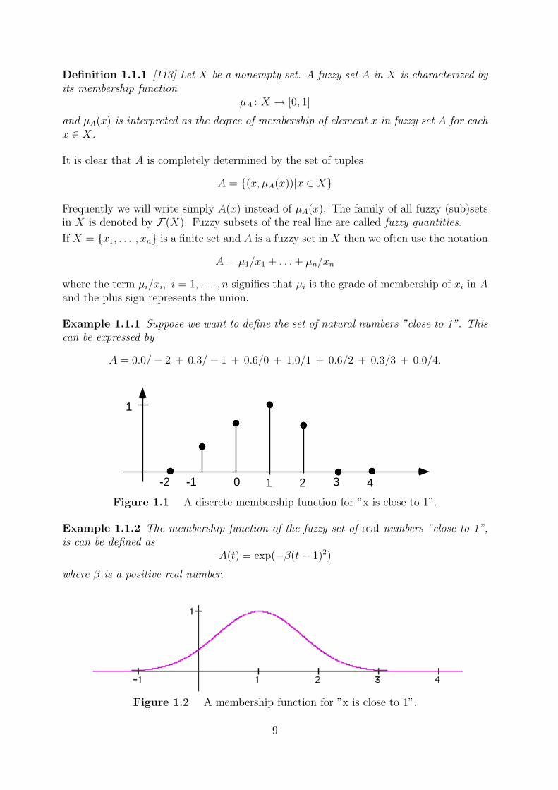
Example 1.1.1 Suppose we want to define the set of natural numbers ”close to 1”. Thiscan be expressed by
A = 0.0/− 2 + 0.3/− 1 + 0.6/0 + 1.0/1 + 0.6/2 + 0.3/3 + 0.0/4.
Figure 1.1 A discrete membership function for ”x is close to 1”.
Example 1.1.2 The membership function of the fuzzy set of real numbers ”close to 1”,is can be defined as
A(t) = exp(−β(t− 1)2)
where β is a positive real number.
Figure 1.2 A membership function for ”x is close to 1”.
9
3000$ 6000$4500$
1
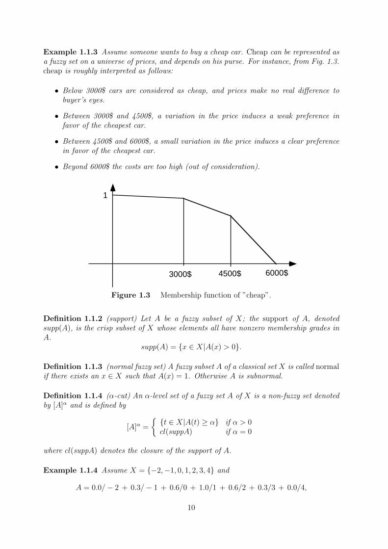
Example 1.1.3 Assume someone wants to buy a cheap car. Cheap can be represented asa fuzzy set on a universe of prices, and depends on his purse. For instance, from Fig. 1.3.cheap is roughly interpreted as follows:
• Below 3000$ cars are considered as cheap, and prices make no real difference tobuyer’s eyes.
• Between 3000$ and 4500$, a variation in the price induces a weak preference infavor of the cheapest car.
• Between 4500$ and 6000$, a small variation in the price induces a clear preferencein favor of the cheapest car.
• Beyond 6000$ the costs are too high (out of consideration).
Figure 1.3 Membership function of ”cheap”.
Definition 1.1.2 (support) Let A be a fuzzy subset of X; the support of A, denotedsupp(A), is the crisp subset of X whose elements all have nonzero membership grades inA.
supp(A) = {x ∈ X|A(x) > 0}.
Definition 1.1.3 (normal fuzzy set) A fuzzy subset A of a classical set X is called normalif there exists an x ∈ X such that A(x) = 1. Otherwise A is subnormal.
Definition 1.1.4 (α-cut) An α-level set of a fuzzy set A of X is a non-fuzzy set denotedby [A]α and is defined by
[A]α =
{{t ∈ X|A(t) ≥ α} if α > 0cl(suppA) if α = 0
where cl(suppA) denotes the closure of the support of A.
Example 1.1.4 Assume X = {−2,−1, 0, 1, 2, 3, 4} and
A = 0.0/− 2 + 0.3/− 1 + 0.6/0 + 1.0/1 + 0.6/2 + 0.3/3 + 0.0/4,
10
αα − cut
in this case
[A]α =
{−1, 0, 1, 2, 3} if 0 ≤ α ≤ 0.3{0, 1, 2} if 0.3 < α ≤ 0.6{1} if 0.6 < α ≤ 1
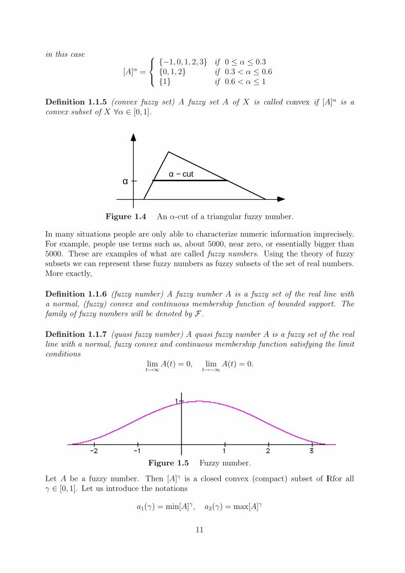
Definition 1.1.5 (convex fuzzy set) A fuzzy set A of X is called convex if [A]α is aconvex subset of X ∀α ∈ [0, 1].
Figure 1.4 An α-cut of a triangular fuzzy number.
In many situations people are only able to characterize numeric information imprecisely.For example, people use terms such as, about 5000, near zero, or essentially bigger than5000. These are examples of what are called fuzzy numbers. Using the theory of fuzzysubsets we can represent these fuzzy numbers as fuzzy subsets of the set of real numbers.More exactly,
Definition 1.1.6 (fuzzy number) A fuzzy number A is a fuzzy set of the real line witha normal, (fuzzy) convex and continuous membership function of bounded support. Thefamily of fuzzy numbers will be denoted by F .
Definition 1.1.7 (quasi fuzzy number) A quasi fuzzy number A is a fuzzy set of the realline with a normal, fuzzy convex and continuous membership function satisfying the limitconditions
limt→∞
A(t) = 0, limt→−∞
A(t) = 0.
Figure 1.5 Fuzzy number.
Let A be a fuzzy number. Then [A]γ is a closed convex (compact) subset of IRfor allγ ∈ [0, 1]. Let us introduce the notations
a1(γ) = min[A]γ, a2(γ) = max[A]γ
11
A
a (0) a (0) 1 2
1γ
a (γ) 1
a (γ) 2
In other words, a1(γ) denotes the left-hand side and a2(γ) denotes the right-hand side ofthe γ-cut. It is easy to see that
If α ≤ β then [A]α ⊃ [A]β
Furthermore, the left-hand side function
a1 : [0, 1]→ IR
is monoton increasing and lower semicontinuous, and the right-hand side function
a2 : [0, 1]→ IR
is monoton decreasing and upper semicontinuous. We shall use the notation
[A]γ = [a1(γ), a2(γ)].
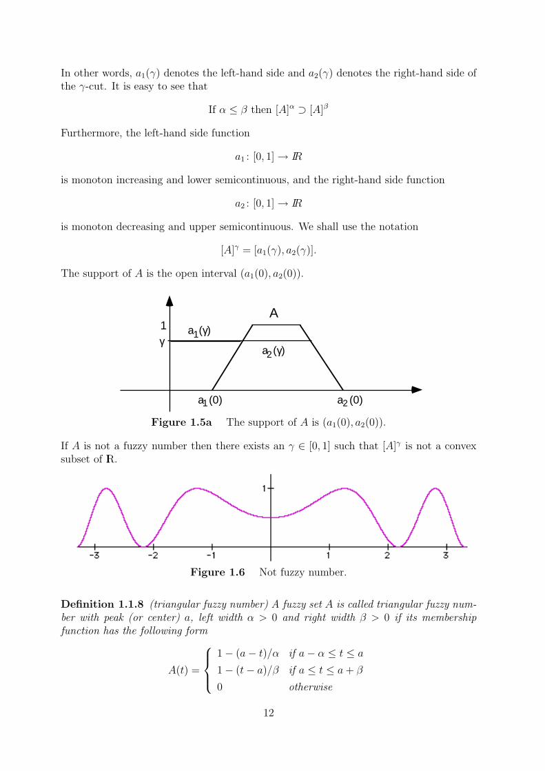
The support of A is the open interval (a1(0), a2(0)).
Figure 1.5a The support of A is (a1(0), a2(0)).
If A is not a fuzzy number then there exists an γ ∈ [0, 1] such that [A]γ is not a convexsubset of IR.
Figure 1.6 Not fuzzy number.
Definition 1.1.8 (triangular fuzzy number) A fuzzy set A is called triangular fuzzy num-ber with peak (or center) a, left width α > 0 and right width β > 0 if its membershipfunction has the following form
A(t) =
1− (a− t)/α if a− α ≤ t ≤ a
1− (t− a)/β if a ≤ t ≤ a+ β
0 otherwise
12
1
aa-α a+β
1
aa- α b+βb
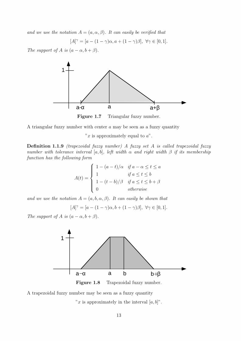
and we use the notation A = (a, α, β). It can easily be verified that
[A]γ = [a− (1− γ)α, a+ (1− γ)β], ∀γ ∈ [0, 1].
The support of A is (a− α, b+ β).
Figure 1.7 Triangular fuzzy number.
A triangular fuzzy number with center a may be seen as a fuzzy quantity
”x is approximately equal to a”.
Definition 1.1.9 (trapezoidal fuzzy number) A fuzzy set A is called trapezoidal fuzzynumber with tolerance interval [a, b], left width α and right width β if its membershipfunction has the following form
A(t) =
1− (a− t)/α if a− α ≤ t ≤ a
1 if a ≤ t ≤ b
1− (t− b)/β if a ≤ t ≤ b+ β
0 otherwise
and we use the notation A = (a, b, α, β). It can easily be shown that
[A]γ = [a− (1− γ)α, b+ (1− γ)β], ∀γ ∈ [0, 1].
The support of A is (a− α, b+ β).
Figure 1.8 Trapezoidal fuzzy number.
A trapezoidal fuzzy number may be seen as a fuzzy quantity
”x is approximately in the interval [a, b]”.
13
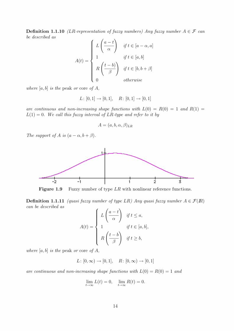
Definition 1.1.10 (LR-representation of fuzzy numbers) Any fuzzy number A ∈ F canbe described as
A(t) =
L
(a− tα
)if t ∈ [a− α, a]
1 if t ∈ [a, b]
R
(t− b)β
)if t ∈ [b, b+ β]
0 otherwise
where [a, b] is the peak or core of A,
L : [0, 1]→ [0, 1], R : [0, 1]→ [0, 1]
are continuous and non-increasing shape functions with L(0) = R(0) = 1 and R(1) =L(1) = 0. We call this fuzzy interval of LR-type and refer to it by
A = (a, b, α, β)LR
The support of A is (a− α, b+ β).
Figure 1.9 Fuzzy number of type LR with nonlinear reference functions.
Definition 1.1.11 (quasi fuzzy number of type LR) Any quasi fuzzy number A ∈ F(IR)can be described as
A(t) =
L
(a− tα
)if t ≤ a,
1 if t ∈ [a, b],
R
(t− bβ
)if t ≥ b,
where [a, b] is the peak or core of A,
L : [0,∞)→ [0, 1], R : [0,∞)→ [0, 1]
are continuous and non-increasing shape functions with L(0) = R(0) = 1 and
limt→∞
L(t) = 0, limt→∞
R(t) = 0.
14
1 - x
B
A
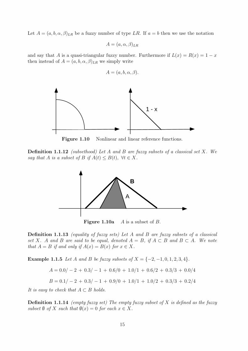
Let A = (a, b, α, β)LR be a fuzzy number of type LR. If a = b then we use the notation
A = (a, α, β)LR
and say that A is a quasi-triangular fuzzy number. Furthermore if L(x) = R(x) = 1− xthen instead of A = (a, b, α, β)LR we simply write
A = (a, b, α, β).
Figure 1.10 Nonlinear and linear reference functions.
Definition 1.1.12 (subsethood) Let A and B are fuzzy subsets of a classical set X. Wesay that A is a subset of B if A(t) ≤ B(t), ∀t ∈ X.
Figure 1.10a A is a subset of B.
Definition 1.1.13 (equality of fuzzy sets) Let A and B are fuzzy subsets of a classicalset X. A and B are said to be equal, denoted A = B, if A ⊂ B and B ⊂ A. We notethat A = B if and only if A(x) = B(x) for x ∈ X.
Example 1.1.5 Let A and B be fuzzy subsets of X = {−2,−1, 0, 1, 2, 3, 4}.
A = 0.0/− 2 + 0.3/− 1 + 0.6/0 + 1.0/1 + 0.6/2 + 0.3/3 + 0.0/4
B = 0.1/− 2 + 0.3/− 1 + 0.9/0 + 1.0/1 + 1.0/2 + 0.3/3 + 0.2/4
It is easy to check that A ⊂ B holds.
Definition 1.1.14 (empty fuzzy set) The empty fuzzy subset of X is defined as the fuzzysubset ∅ of X such that ∅(x) = 0 for each x ∈ X.
15
10
X 1
x
1
1
x0
x0_
It is easy to see that ∅ ⊂ A holds for any fuzzy subset A of X.
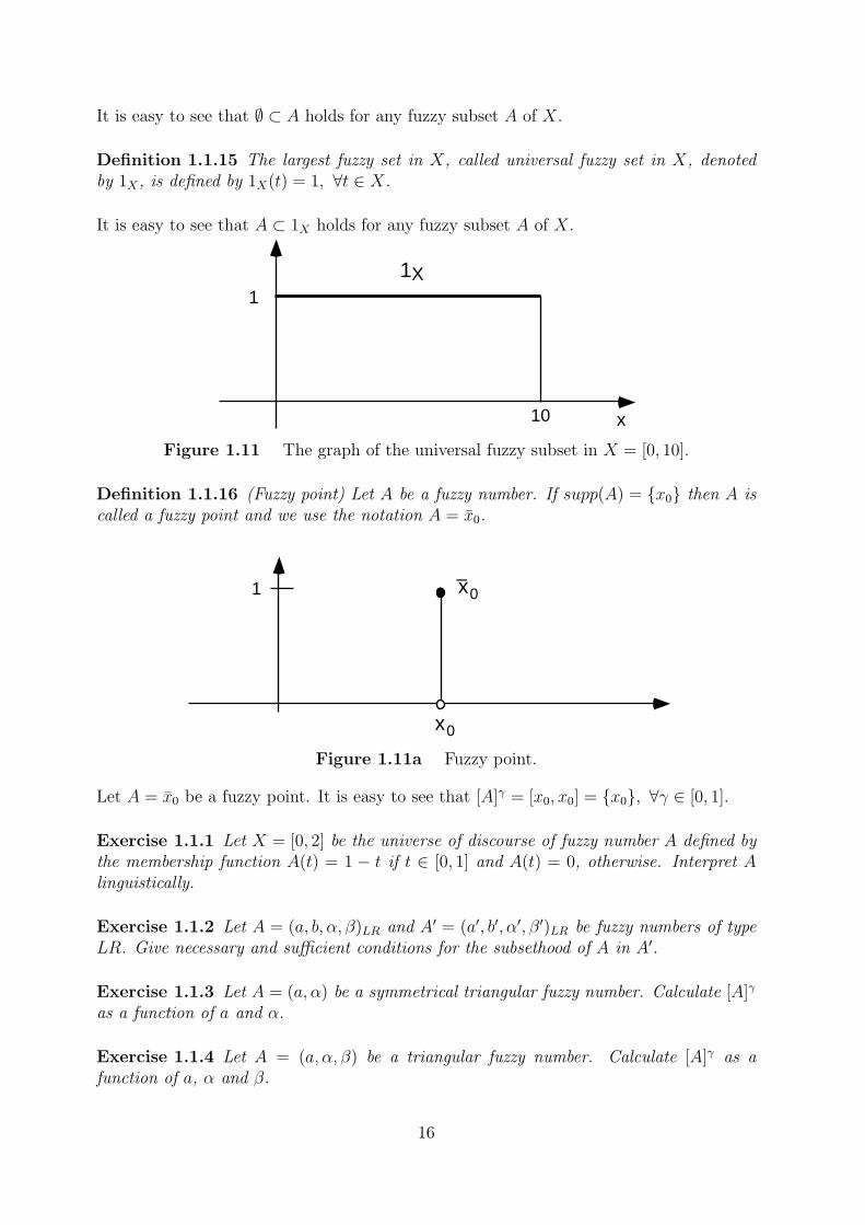
Definition 1.1.15 The largest fuzzy set in X, called universal fuzzy set in X, denotedby 1X , is defined by 1X(t) = 1, ∀t ∈ X.
It is easy to see that A ⊂ 1X holds for any fuzzy subset A of X.
Figure 1.11 The graph of the universal fuzzy subset in X = [0, 10].
Definition 1.1.16 (Fuzzy point) Let A be a fuzzy number. If supp(A) = {x0} then A iscalled a fuzzy point and we use the notation A = x0.
Figure 1.11a Fuzzy point.
Let A = x0 be a fuzzy point. It is easy to see that [A]γ = [x0, x0] = {x0}, ∀γ ∈ [0, 1].
Exercise 1.1.1 Let X = [0, 2] be the universe of discourse of fuzzy number A defined bythe membership function A(t) = 1 − t if t ∈ [0, 1] and A(t) = 0, otherwise. Interpret Alinguistically.
Exercise 1.1.2 Let A = (a, b, α, β)LR and A′ = (a′, b′, α′, β′)LR be fuzzy numbers of typeLR. Give necessary and sufficient conditions for the subsethood of A in A′.
Exercise 1.1.3 Let A = (a, α) be a symmetrical triangular fuzzy number. Calculate [A]γ
as a function of a and α.
Exercise 1.1.4 Let A = (a, α, β) be a triangular fuzzy number. Calculate [A]γ as afunction of a, α and β.
16

Exercise 1.1.5 Let A = (a, b, α, β) be a trapezoidal fuzzy number. Calculate [A]γ as afunction of a, b, α and β.
Exercise 1.1.6 Let A = (a, b, α, β)LR be a fuzzy number of type LR. Calculate [A]γ as afunction of a, b, α, β, L and R.
17
A B
1.2 Operations on fuzzy sets
In this section we extend the classical set theoretic operations from ordinary set theoryto fuzzy sets. We note that all those operations which are extensions of crisp conceptsreduce to their usual meaning when the fuzzy subsets have membership degrees that aredrawn from {0, 1}. For this reason, when extending operations to fuzzy sets we use thesame symbol as in set theory.
Let A and B are fuzzy subsets of a nonempty (crisp) set X.
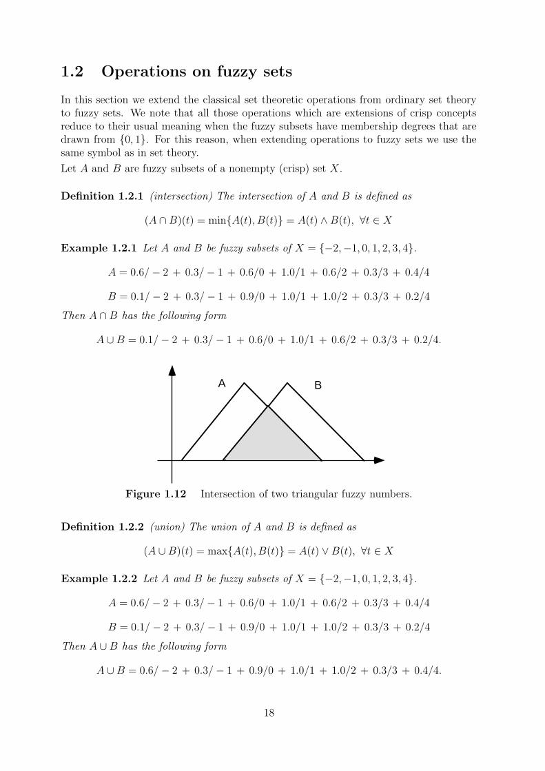
Definition 1.2.1 (intersection) The intersection of A and B is defined as
(A ∩B)(t) = min{A(t), B(t)} = A(t) ∧B(t), ∀t ∈ X
Example 1.2.1 Let A and B be fuzzy subsets of X = {−2,−1, 0, 1, 2, 3, 4}.
A = 0.6/− 2 + 0.3/− 1 + 0.6/0 + 1.0/1 + 0.6/2 + 0.3/3 + 0.4/4
B = 0.1/− 2 + 0.3/− 1 + 0.9/0 + 1.0/1 + 1.0/2 + 0.3/3 + 0.2/4
Then A ∩B has the following form
A ∪B = 0.1/− 2 + 0.3/− 1 + 0.6/0 + 1.0/1 + 0.6/2 + 0.3/3 + 0.2/4.
Figure 1.12 Intersection of two triangular fuzzy numbers.
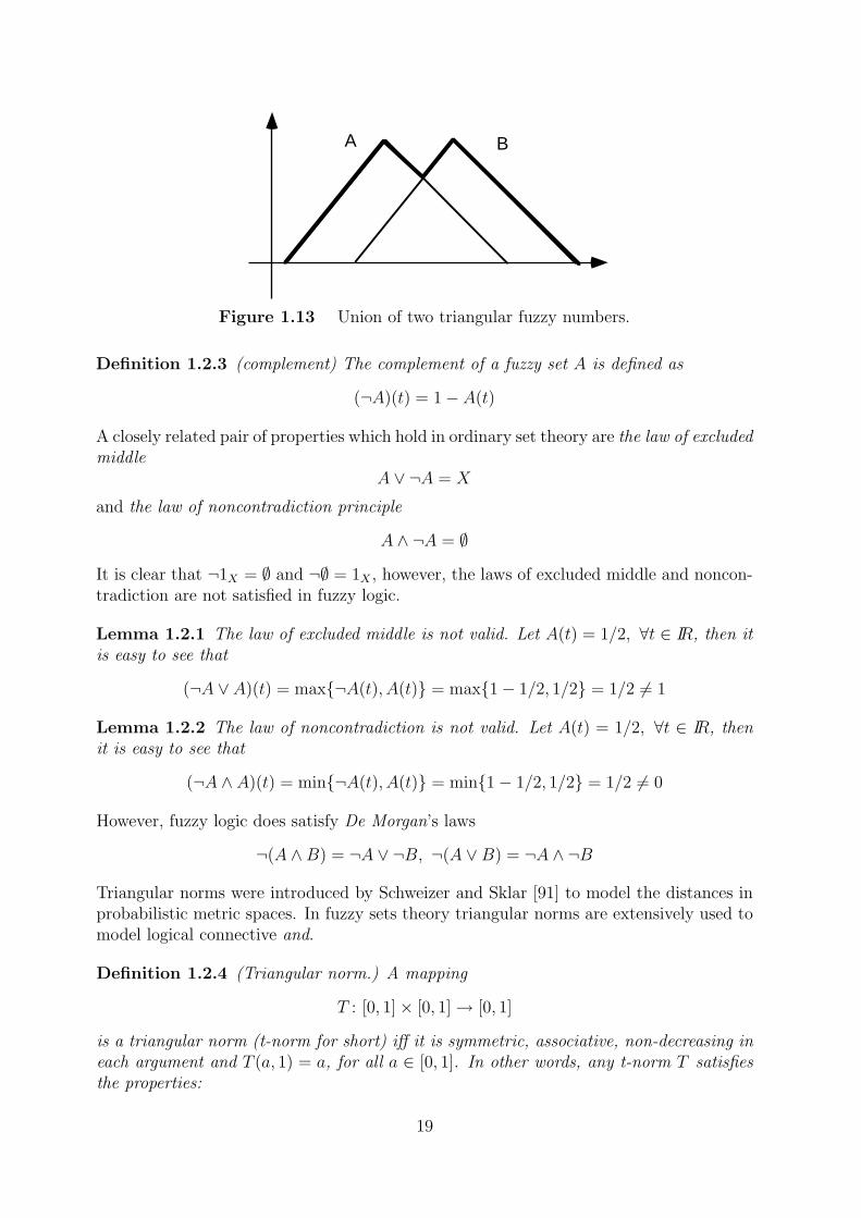
Definition 1.2.2 (union) The union of A and B is defined as
(A ∪B)(t) = max{A(t), B(t)} = A(t) ∨B(t), ∀t ∈ X
Example 1.2.2 Let A and B be fuzzy subsets of X = {−2,−1, 0, 1, 2, 3, 4}.
A = 0.6/− 2 + 0.3/− 1 + 0.6/0 + 1.0/1 + 0.6/2 + 0.3/3 + 0.4/4
B = 0.1/− 2 + 0.3/− 1 + 0.9/0 + 1.0/1 + 1.0/2 + 0.3/3 + 0.2/4
Then A ∪B has the following form
A ∪B = 0.6/− 2 + 0.3/− 1 + 0.9/0 + 1.0/1 + 1.0/2 + 0.3/3 + 0.4/4.
18
A B
Figure 1.13 Union of two triangular fuzzy numbers.
Definition 1.2.3 (complement) The complement of a fuzzy set A is defined as
(¬A)(t) = 1− A(t)
A closely related pair of properties which hold in ordinary set theory are the law of excludedmiddle
A ∨ ¬A = X
and the law of noncontradiction principle
A ∧ ¬A = ∅
It is clear that ¬1X = ∅ and ¬∅ = 1X , however, the laws of excluded middle and noncon-tradiction are not satisfied in fuzzy logic.
Lemma 1.2.1 The law of excluded middle is not valid. Let A(t) = 1/2, ∀t ∈ IR, then itis easy to see that
(¬A ∨ A)(t) = max{¬A(t), A(t)} = max{1− 1/2, 1/2} = 1/2 6= 1
Lemma 1.2.2 The law of noncontradiction is not valid. Let A(t) = 1/2, ∀t ∈ IR, thenit is easy to see that
(¬A ∧ A)(t) = min{¬A(t), A(t)} = min{1− 1/2, 1/2} = 1/2 6= 0
However, fuzzy logic does satisfy De Morgan’s laws
¬(A ∧B) = ¬A ∨ ¬B, ¬(A ∨B) = ¬A ∧ ¬B
Triangular norms were introduced by Schweizer and Sklar [91] to model the distances inprobabilistic metric spaces. In fuzzy sets theory triangular norms are extensively used tomodel logical connective and.
Definition 1.2.4 (Triangular norm.) A mapping
T : [0, 1]× [0, 1]→ [0, 1]
is a triangular norm (t-norm for short) iff it is symmetric, associative, non-decreasing ineach argument and T (a, 1) = a, for all a ∈ [0, 1]. In other words, any t-norm T satisfiesthe properties:
19
T (x, y) = T (y, x) (symmetricity)
T (x, T (y, z)) = T (T (x, y), z) (associativity)
T (x, y) ≤ T (x′, y′) if x ≤ x′ and y ≤ y′ (monotonicity)
T (x, 1) = x, ∀x ∈ [0, 1] (one identy)
All t-norms may be extended, through associativity, to n > 2 arguments. The t-normMIN is automatically extended and
PAND(a1, . . . , an) = a1a2 · · · an
LAND(a1, . . . an) = max{n∑i=1
ai − n+ 1, 0}
A t-norm T is called strict if T is strictly increasing in each argument.
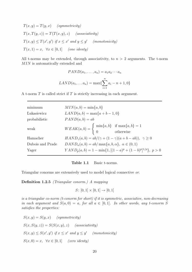
minimum MIN(a, b) = min{a, b}ÃLukasiewicz LAND(a, b) = max{a+ b− 1, 0}probabilistic PAND(a, b) = ab
weak WEAK(a, b) =
{min{a, b} if max{a, b} = 1
0 otherwise
Hamacher HANDγ(a, b) = ab/(γ + (1− γ)(a+ b− ab)), γ ≥ 0
Dubois and Prade DANDα(a, b) = ab/max{a, b, α}, α ∈ (0, 1)
Yager Y ANDp(a, b) = 1−min{1, [(1− a)p + (1− b)p]1/p}, p > 0
Table 1.1 Basic t-norms.
Triangular conorms are extensively used to model logical connective or.
Definition 1.2.5 (Triangular conorm.) A mapping
S : [0, 1]× [0, 1]→ [0, 1]
is a triangular co-norm (t-conorm for short) if it is symmetric, associative, non-decreasingin each argument and S(a, 0) = a, for all a ∈ [0, 1]. In other words, any t-conorm Ssatisfies the properties:
S(x, y) = S(y, x) (symmetricity)
S(x, S(y, z)) = S(S(x, y), z) (associativity)
S(x, y) ≤ S(x′, y′) if x ≤ x′ and y ≤ y′ (monotonicity)
S(x, 0) = x, ∀x ∈ [0, 1] (zero identy)
20
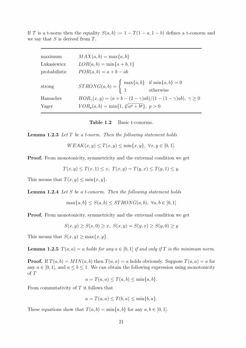
If T is a t-norm then the equality S(a, b) := 1 − T (1 − a, 1 − b) defines a t-conorm andwe say that S is derived from T .
maximum MAX(a, b) = max{a, b}ÃLukasiewicz LOR(a, b) = min{a+ b, 1}probabilistic POR(a, b) = a+ b− ab
strong STRONG(a, b) =
{max{a, b} if min{a, b} = 0
1 otherwise
Hamacher HORγ(x, y) = (a+ b− (2− γ)ab)/(1− (1− γ)ab), γ ≥ 0
Yager Y ORp(a, b) = min{1, p√ap + bp}, p > 0
Table 1.2 Basic t-conorms.
Lemma 1.2.3 Let T be a t-norm. Then the following statement holds
WEAK(x, y) ≤ T (x, y) ≤ min{x, y}, ∀x, y ∈ [0, 1].
Proof. From monotonicity, symmetricity and the extremal condition we get
T (x, y) ≤ T (x, 1) ≤ x, T (x, y) = T (y, x) ≤ T (y, 1) ≤ y.
This means that T (x, y) ≤ min{x, y}.
Lemma 1.2.4 Let S be a t-conorm. Then the following statement holds
max{a, b} ≤ S(a, b) ≤ STRONG(a, b), ∀a, b ∈ [0, 1]
Proof. From monotonicity, symmetricity and the extremal condition we get
S(x, y) ≥ S(x, 0) ≥ x, S(x, y) = S(y, x) ≥ S(y, 0) ≥ y
This means that S(x, y) ≥ max{x, y}.
Lemma 1.2.5 T (a, a) = a holds for any a ∈ [0, 1] if and only if T is the minimum norm.
Proof. If T (a, b) = MIN(a, b) then T (a, a) = a holds obviously. Suppose T (a, a) = a forany a ∈ [0, 1], and a ≤ b ≤ 1. We can obtain the following expression using monotonicityof T
a = T (a, a) ≤ T (a, b) ≤ min{a, b}.From commutativity of T it follows that
a = T (a, a) ≤ T (b, a) ≤ min{b, a}.
These equations show that T (a, b) = min{a, b} for any a, b ∈ [0, 1].
21
Lemma 1.2.6 The distributive law of T on the max operator holds for any a, b, c ∈ [0, 1].
T (max{a, b}, c) = max{T (a, c), T (b, c)}.
The operation intersection can be defined by the help of triangular norms.
Definition 1.2.6 (t-norm-based intersection) Let T be a t-norm. The T -intersection ofA and B is defined as
(A ∩B)(t) = T (A(t), B(t)), ∀t ∈ X.
Example 1.2.3 Let T (x, y) = max{x + y − 1, 0} be the ÃLukasiewicz t-norm. Then wehave
(A ∩B)(t) = max{A(t) +B(t)− 1, 0} ∀t ∈ X.
Let A and B be fuzzy subsets of X = {−2,−1, 0, 1, 2, 3, 4}.
A = 0.0/− 2 + 0.3/− 1 + 0.6/0 + 1.0/1 + 0.6/2 + 0.3/3 + 0.0/4
B = 0.1/− 2 + 0.3/− 1 + 0.9/0 + 1.0/1 + 1.0/2 + 0.3/3 + 0.2/4
Then A ∩B has the following form
A ∩B = 0.0/− 2 + 0.0/− 1 + 0.5/0 + 1.0/1 + 0.6/2 + 0.0/3 + 0.2/4
The operation union can be defined by the help of triangular conorms.
Definition 1.2.7 (t-conorm-based union) Let S be a t-conorm. The S-union of A andB is defined as
(A ∪B)(t) = S(A(t), B(t)), ∀t ∈ X.
Example 1.2.4 Let S(x, y) = min{x+ y, 1} be the ÃLukasiewicz t-conorm. Then we have
(A ∪B)(t) = min{A(t) +B(t), 1}, ∀t ∈ X.
Let A and B be fuzzy subsets of X = {−2,−1, 0, 1, 2, 3, 4}.
A = 0.0/− 2 + 0.3/− 1 + 0.6/0 + 1.0/1 + 0.6/2 + 0.3/3 + 0.0/4
B = 0.1/− 2 + 0.3/− 1 + 0.9/0 + 1.0/1 + 1.0/2 + 0.3/3 + 0.0/4
Then A ∪B has the following form
A ∪B = 0.1/− 2 + 0.6/− 1 + 1.0/0 + 1.0/1 + 1.0/2 + 0.6/3 + 0.2/4.
In general, the law of the excluded middle and the noncontradiction principle propertiesare not satisfied by t-norms and t-conorms defining the intersection and union operations.However, the ÃLukasiewicz t-norm and t-conorm do satisfy these properties.
Lemma 1.2.7 If T (x, y) = LAND(x, y) = max{x+ y− 1, 0} then the law of noncontra-diction is valid.
22
Proof. Let A be a fuzzy set in X. Then from the definition of t-norm-based intersectionwe get
(A ∩ ¬A)(t) = LAND(A(t), 1− A(t)) = (A(t) + 1− A(t)− 1) ∨ 0 = 0, ∀t ∈ X.
Lemma 1.2.8 If S(x, y) = LOR(x, y) = min{1, x + y} then the law of excluded middleis valid.
Proof.Let A be a fuzzy set in X. Then from the definition of t-conorm-based union weget
(A ∪ ¬A)(t) = LOR(A(t), 1− A(t)) = (A(t) + 1− A(t)) ∧ 1 = 1, ∀t ∈ X.
Exercise 1.2.1 Let A and B be fuzzy subsets of X = {−2,−1, 0, 1, 2, 3, 4}.
A = 0.5/− 2 + 0.4/− 1 + 0.6/0 + 1.0/1 + 0.6/2 + 0.3/3 + 0.4/4
B = 0.1/− 2 + 0.7/− 1 + 0.9/0 + 1.0/1 + 1.0/2 + 0.3/3 + 0.2/4
Suppose that their intersection is defined by the probabilistic t-norm PAND(a, b) = ab.What is then the membership function of A ∩B?
Exercise 1.2.2 Let A and B be fuzzy subsets of X = {−2,−1, 0, 1, 2, 3, 4}.
A = 0.5/− 2 + 0.4/− 1 + 0.6/0 + 1.0/1 + 0.6/2 + 0.3/3 + 0.4/4
B = 0.1/− 2 + 0.7/− 1 + 0.9/0 + 1.0/1 + 1.0/2 + 0.3/3 + 0.2/4
Suppose that their union is defined by the probabilistic t-conorm PAND(a, b) = a+b−ab.What is then the membership function of A ∪B?
Exercise 1.2.3 Let A and B be fuzzy subsets of X = {−2,−1, 0, 1, 2, 3, 4}.
A = 0.7/− 2 + 0.4/− 1 + 0.6/0 + 1.0/1 + 0.6/2 + 0.3/3 + 0.4/4
B = 0.1/− 2 + 0.2/− 1 + 0.9/0 + 1.0/1 + 1.0/2 + 0.3/3 + 0.2/4
Suppose that their intersection is defined by the Hamacher’s t-norm with γ = 0. What isthen the membership function of A ∩B?
Exercise 1.2.4 Let A and B be fuzzy subsets of X = {−2,−1, 0, 1, 2, 3, 4}.
A = 0.7/− 2 + 0.4/− 1 + 0.6/0 + 1.0/1 + 0.6/2 + 0.3/3 + 0.4/4
B = 0.1/− 2 + 0.2/− 1 + 0.9/0 + 1.0/1 + 1.0/2 + 0.3/3 + 0.2/4
Suppose that their intersection is defined by the Hamacher’s t-conorm with γ = 0. Whatis then the membership function of A ∪B?
Exercise 1.2.5 Show that if γ ≤ γ′ then HANDγ(x, y) ≥ HANDγ′(x, y) holds for allx, y ∈ [0, 1], i.e. the family HANDγ is monoton decreasing.
23
ba
c
1.3 Fuzzy relations
A classical relation can be considered as a set of tuples, where a tuple is an ordered pair.A binary tuple is denoted by (u, v), an example of a ternary tuple is (u, v, w) and anexample of n-ary tuple is (x1, . . . , xn).
Definition 1.3.1 (classical n-ary relation) Let X1, . . . , Xn be classical sets. The subsetsof the Cartesian product X1 × · · · ×Xn are called n-ary relations. If X1 = · · · = Xn andR ⊂ Xn then R is called an n-ary relation in X.
Let R be a binary relation in IR. Then the characteristic function of R is defined as
χR(u, v) =
{1 if (u, v) ∈ R0 otherwise
Example 1.3.1 Let X be the domain of men {John, Charles, James} and Y the domainof women {Diana, Rita, Eva}, then the relation ”married to” on X × Y is, for example
{(Charles, Diana), (John, Eva), (James, Rita) }
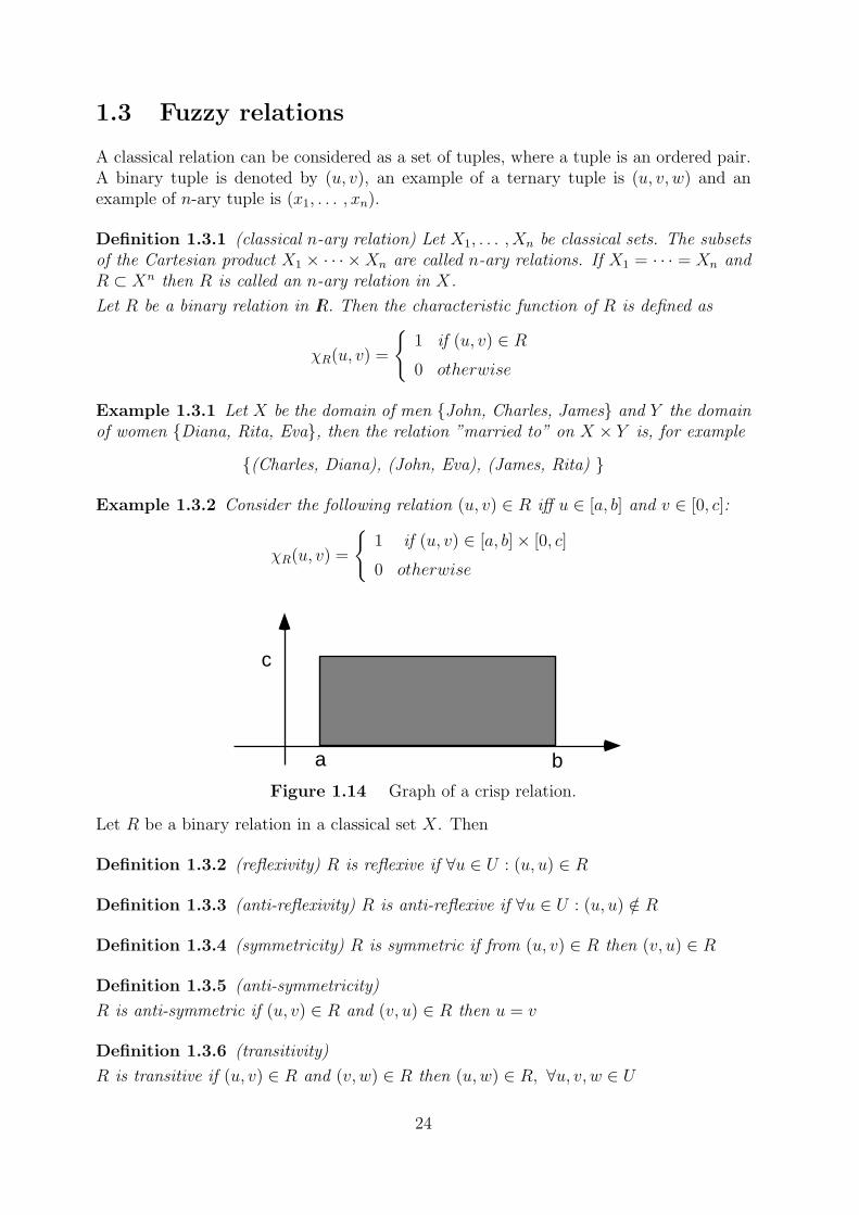
Example 1.3.2 Consider the following relation (u, v) ∈ R iff u ∈ [a, b] and v ∈ [0, c]:
χR(u, v) =
{1 if (u, v) ∈ [a, b]× [0, c]
0 otherwise
Figure 1.14 Graph of a crisp relation.
Let R be a binary relation in a classical set X. Then
Definition 1.3.2 (reflexivity) R is reflexive if ∀u ∈ U : (u, u) ∈ R
Definition 1.3.3 (anti-reflexivity) R is anti-reflexive if ∀u ∈ U : (u, u) /∈ R
Definition 1.3.4 (symmetricity) R is symmetric if from (u, v) ∈ R then (v, u) ∈ R
Definition 1.3.5 (anti-symmetricity)
R is anti-symmetric if (u, v) ∈ R and (v, u) ∈ R then u = v
Definition 1.3.6 (transitivity)
R is transitive if (u, v) ∈ R and (v, w) ∈ R then (u,w) ∈ R, ∀u, v, w ∈ U
24
Example 1.3.3 Consider the classical inequality relations on the real line IR. It is clearthat ≤ is reflexive, anti-symmetric and transitive, while < is anti-reflexive, anti-symmetric and transitive.
Other important classes of binary relations are the following:
Definition 1.3.7 (equivalence) R is an equivalence relation if, R is reflexive, symmetricand transitive
Definition 1.3.8 (partial order) R is a partial order relation if it is reflexive, anti-sym-metric and transitive
Definition 1.3.9 (total order) R is a total order relation if it is partial order and (u, v) ∈R or (v, u) ∈ R hold for any u and v.
Example 1.3.4 Let us consider the binary relation ”subset of”. It is clear that it is apartial order relation. The relation ≤ on natural numbers is a total order relation.
Example 1.3.5 Consider the relation ”mod 3” on natural numbers
{(m,n) | (n−m) mod 3 ≡ 0}
This is an equivalence relation.
Definition 1.3.10 (fuzzy relation) Let X and Y be nonempty sets. A fuzzy relation Ris a fuzzy subset of X × Y . In other words, R ∈ F(X × Y ). If X = Y then we say thatR is a binary fuzzy relation in X.
Let R be a binary fuzzy relation on IR. Then R(u, v) is interpreted as the degree ofmembership of (u, v) in R.
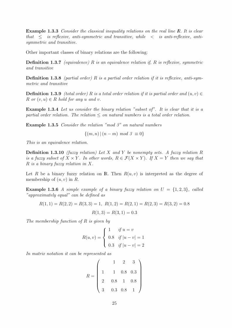
Example 1.3.6 A simple example of a binary fuzzy relation on U = {1, 2, 3}, called”approximately equal” can be defined as
R(1, 1) = R(2, 2) = R(3, 3) = 1, R(1, 2) = R(2, 1) = R(2, 3) = R(3, 2) = 0.8
R(1, 3) = R(3, 1) = 0.3
The membership function of R is given by
R(u, v) =
1 if u = v
0.8 if |u− v| = 1
0.3 if |u− v| = 2
In matrix notation it can be represented as
R =
1 2 3
1 1 0.8 0.3
2 0.8 1 0.8
3 0.3 0.8 1
25
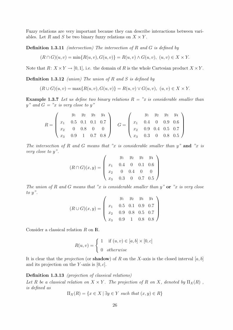
Fuzzy relations are very important because they can describe interactions between vari-ables. Let R and S be two binary fuzzy relations on X × Y .
Definition 1.3.11 (intersection) The intersection of R and G is defined by
(R ∩G)(u, v) = min{R(u, v), G(u, v)} = R(u, v) ∧G(u, v), (u, v) ∈ X × Y.
Note that R : X×Y → [0, 1], i.e. the domain of R is the whole Cartesian product X×Y .
Definition 1.3.12 (union) The union of R and S is defined by
(R ∪G)(u, v) = max{R(u, v), G(u, v)} = R(u, v) ∨G(u, v), (u, v) ∈ X × Y.
Example 1.3.7 Let us define two binary relations R = ”x is considerable smaller thany” and G = ”x is very close to y”
R =
y1 y2 y3 y4
x1 0.5 0.1 0.1 0.7
x2 0 0.8 0 0
x3 0.9 1 0.7 0.8
G =
y1 y2 y3 y4
x1 0.4 0 0.9 0.6
x2 0.9 0.4 0.5 0.7
x3 0.3 0 0.8 0.5
The intersection of R and G means that ”x is considerable smaller than y” and ”x isvery close to y”.
(R ∩G)(x, y) =
y1 y2 y3 y4
x1 0.4 0 0.1 0.6
x2 0 0.4 0 0
x3 0.3 0 0.7 0.5
The union of R and G means that ”x is considerable smaller than y” or ”x is very closeto y”.
(R ∪G)(x, y) =
y1 y2 y3 y4
x1 0.5 0.1 0.9 0.7
x2 0.9 0.8 0.5 0.7
x3 0.9 1 0.8 0.8
Consider a classical relation R on IR.
R(u, v) =
{1 if (u, v) ∈ [a, b]× [0, c]
0 otherwise
It is clear that the projection (or shadow) of R on the X-axis is the closed interval [a, b]and its projection on the Y -axis is [0, c].
Definition 1.3.13 (projection of classical relations)
Let R be a classical relation on X × Y . The projection of R on X, denoted by ΠX(R) ,is defined as
ΠX(R) = {x ∈ X | ∃y ∈ Y such that (x, y) ∈ R}
26
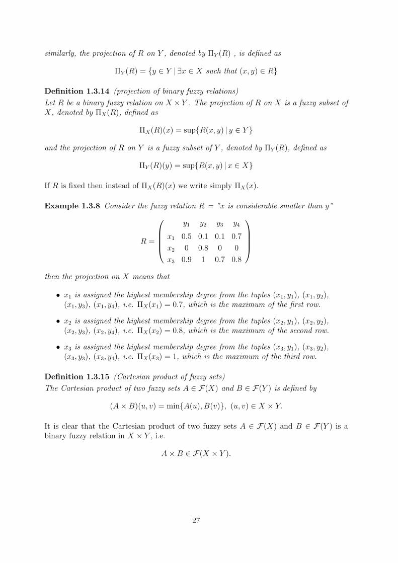
similarly, the projection of R on Y , denoted by ΠY (R) , is defined as
ΠY (R) = {y ∈ Y | ∃x ∈ X such that (x, y) ∈ R}
Definition 1.3.14 (projection of binary fuzzy relations)
Let R be a binary fuzzy relation on X × Y . The projection of R on X is a fuzzy subset ofX, denoted by ΠX(R), defined as
ΠX(R)(x) = sup{R(x, y) | y ∈ Y }
and the projection of R on Y is a fuzzy subset of Y , denoted by ΠY (R), defined as
ΠY (R)(y) = sup{R(x, y) |x ∈ X}
If R is fixed then instead of ΠX(R)(x) we write simply ΠX(x).
Example 1.3.8 Consider the fuzzy relation R = ”x is considerable smaller than y”
R =
y1 y2 y3 y4
x1 0.5 0.1 0.1 0.7
x2 0 0.8 0 0
x3 0.9 1 0.7 0.8
then the projection on X means that
• x1 is assigned the highest membership degree from the tuples (x1, y1), (x1, y2),(x1, y3), (x1, y4), i.e. ΠX(x1) = 0.7, which is the maximum of the first row.
• x2 is assigned the highest membership degree from the tuples (x2, y1), (x2, y2),(x2, y3), (x2, y4), i.e. ΠX(x2) = 0.8, which is the maximum of the second row.
• x3 is assigned the highest membership degree from the tuples (x3, y1), (x3, y2),(x3, y3), (x3, y4), i.e. ΠX(x3) = 1, which is the maximum of the third row.
Definition 1.3.15 (Cartesian product of fuzzy sets)
The Cartesian product of two fuzzy sets A ∈ F(X) and B ∈ F(Y ) is defined by
(A×B)(u, v) = min{A(u), B(v)}, (u, v) ∈ X × Y.
It is clear that the Cartesian product of two fuzzy sets A ∈ F(X) and B ∈ F(Y ) is abinary fuzzy relation in X × Y , i.e.
A×B ∈ F(X × Y ).
27
A x B
A
B
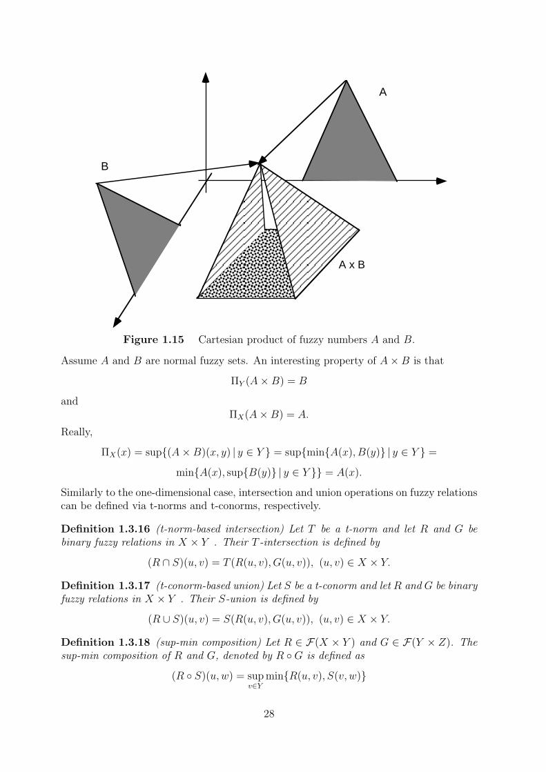
Figure 1.15 Cartesian product of fuzzy numbers A and B.
Assume A and B are normal fuzzy sets. An interesting property of A×B is that
ΠY (A×B) = B
andΠX(A×B) = A.
Really,
ΠX(x) = sup{(A×B)(x, y) | y ∈ Y } = sup{min{A(x), B(y)} | y ∈ Y } =
min{A(x), sup{B(y)} | y ∈ Y }} = A(x).
Similarly to the one-dimensional case, intersection and union operations on fuzzy relationscan be defined via t-norms and t-conorms, respectively.
Definition 1.3.16 (t-norm-based intersection) Let T be a t-norm and let R and G bebinary fuzzy relations in X × Y . Their T -intersection is defined by
(R ∩ S)(u, v) = T (R(u, v), G(u, v)), (u, v) ∈ X × Y.
Definition 1.3.17 (t-conorm-based union) Let S be a t-conorm and let R and G be binaryfuzzy relations in X × Y . Their S-union is defined by
(R ∪ S)(u, v) = S(R(u, v), G(u, v)), (u, v) ∈ X × Y.
Definition 1.3.18 (sup-min composition) Let R ∈ F(X × Y ) and G ∈ F(Y × Z). Thesup-min composition of R and G, denoted by R ◦G is defined as
(R ◦ S)(u,w) = supv∈Y
min{R(u, v), S(v, w)}
28
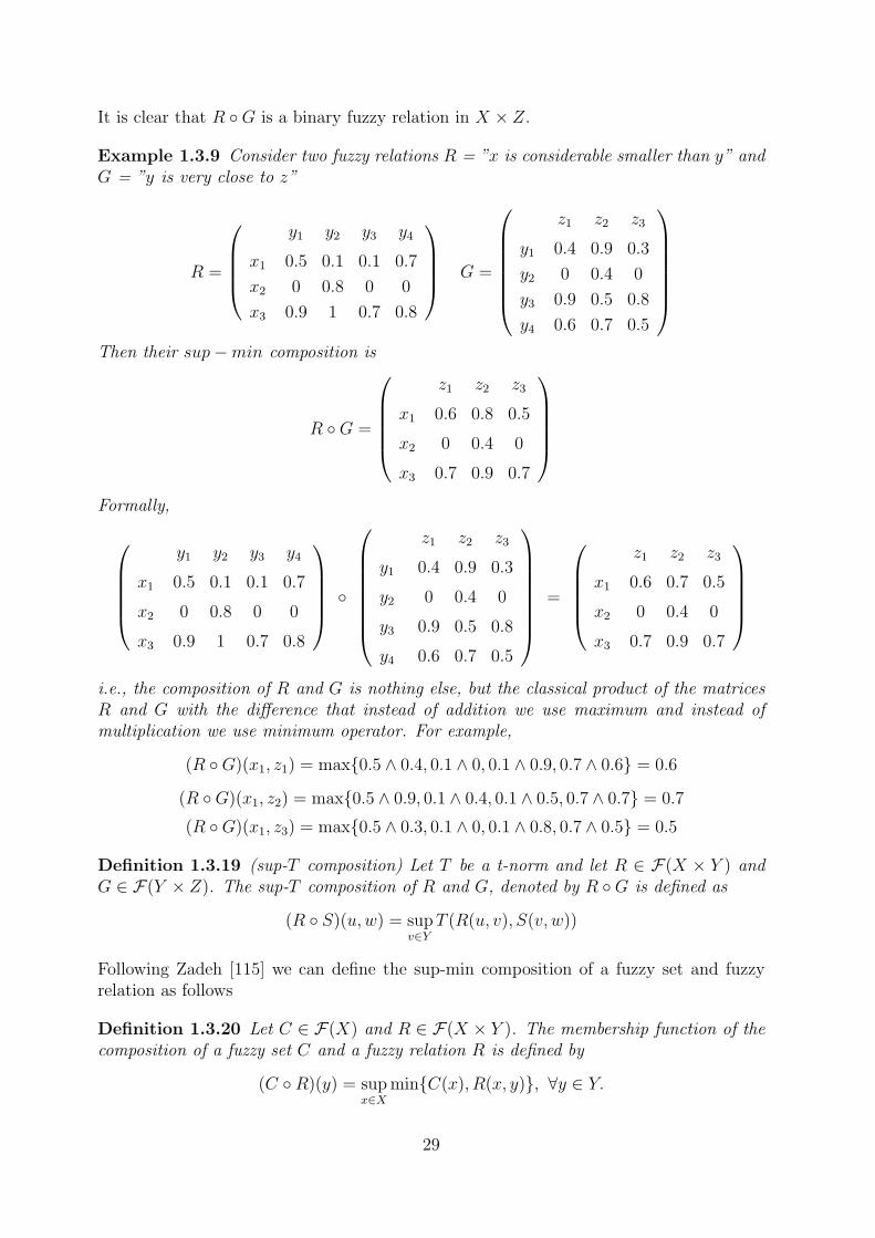
It is clear that R ◦G is a binary fuzzy relation in X × Z.
Example 1.3.9 Consider two fuzzy relations R = ”x is considerable smaller than y” andG = ”y is very close to z”
R =
y1 y2 y3 y4
x1 0.5 0.1 0.1 0.7
x2 0 0.8 0 0
x3 0.9 1 0.7 0.8
G =
z1 z2 z3
y1 0.4 0.9 0.3
y2 0 0.4 0
y3 0.9 0.5 0.8
y4 0.6 0.7 0.5
Then their sup−min composition is
R ◦G =
z1 z2 z3
x1 0.6 0.8 0.5
x2 0 0.4 0
x3 0.7 0.9 0.7
Formally,
y1 y2 y3 y4
x1 0.5 0.1 0.1 0.7
x2 0 0.8 0 0
x3 0.9 1 0.7 0.8
◦
z1 z2 z3
y1 0.4 0.9 0.3
y2 0 0.4 0
y3 0.9 0.5 0.8
y4 0.6 0.7 0.5
=
z1 z2 z3
x1 0.6 0.7 0.5
x2 0 0.4 0
x3 0.7 0.9 0.7
i.e., the composition of R and G is nothing else, but the classical product of the matricesR and G with the difference that instead of addition we use maximum and instead ofmultiplication we use minimum operator. For example,
(R ◦G)(x1, z1) = max{0.5 ∧ 0.4, 0.1 ∧ 0, 0.1 ∧ 0.9, 0.7 ∧ 0.6} = 0.6
(R ◦G)(x1, z2) = max{0.5 ∧ 0.9, 0.1 ∧ 0.4, 0.1 ∧ 0.5, 0.7 ∧ 0.7} = 0.7
(R ◦G)(x1, z3) = max{0.5 ∧ 0.3, 0.1 ∧ 0, 0.1 ∧ 0.8, 0.7 ∧ 0.5} = 0.5
Definition 1.3.19 (sup-T composition) Let T be a t-norm and let R ∈ F(X × Y ) andG ∈ F(Y × Z). The sup-T composition of R and G, denoted by R ◦G is defined as
(R ◦ S)(u,w) = supv∈Y
T (R(u, v), S(v, w))
Following Zadeh [115] we can define the sup-min composition of a fuzzy set and fuzzyrelation as follows
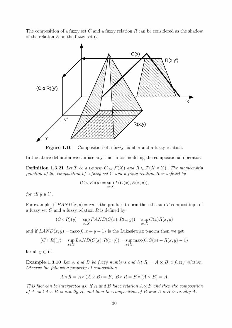
Definition 1.3.20 Let C ∈ F(X) and R ∈ F(X × Y ). The membership function of thecomposition of a fuzzy set C and a fuzzy relation R is defined by
(C ◦R)(y) = supx∈X
min{C(x), R(x, y)}, ∀y ∈ Y.
29
Y
X
y'R(x,y)
(C o R)(y')
R(x,y') C(x)
The composition of a fuzzy set C and a fuzzy relation R can be considered as the shadowof the relation R on the fuzzy set C.
Figure 1.16 Composition of a fuzzy number and a fuzzy relation.
In the above definition we can use any t-norm for modeling the compositional operator.
Definition 1.3.21 Let T be a t-norm C ∈ F(X) and R ∈ F(X × Y ). The membershipfunction of the composition of a fuzzy set C and a fuzzy relation R is defined by
(C ◦R)(y) = supx∈X
T (C(x), R(x, y)),
for all y ∈ Y .
For example, if PAND(x, y) = xy is the product t-norm then the sup-T compositiopn ofa fuzzy set C and a fuzzy relation R is defined by
(C ◦R)(y) = supx∈X
PAND(C(x), R(x, y)) = supx∈X
C(x)R(x, y)
and if LAND(x, y) = max{0, x+ y − 1} is the ÃLukasiewicz t-norm then we get
(C ◦R)(y) = supx∈X
LAND(C(x), R(x, y)) = supx∈X
max{0, C(x) +R(x, y)− 1}
for all y ∈ Y .
Example 1.3.10 Let A and B be fuzzy numbers and let R = A × B a fuzzy relation.Observe the following property of composition
A ◦R = A ◦ (A×B) = B, B ◦R = B ◦ (A×B) = A.
This fact can be interpreted as: if A and B have relation A×B and then the compositionof A and A×B is exactly B, and then the composition of B and A×B is exactly A.
30
Example 1.3.11 Let C be a fuzzy set in the universe of discourse {1, 2, 3} and let R bea binary fuzzy relation in {1, 2, 3}. Assume that C = 0.2/1 + 1/2 + 0.2/3 and
R =
1 2 3
1 1 0.8 0.3
2 0.8 1 0.8
3 0.3 0.8 1
Using Definition 1.3.20 we get
C ◦R = (0.2/1 + 1/2 + 0.2/3) ◦
1 2 3
1 1 0.8 0.3
2 0.8 1 0.8
3 0.3 0.8 1
= 0.8/1 + 1/2 + 0.8/3.
Example 1.3.12 Let C be a fuzzy set in the universe of discourse [0, 1] and let R be abinary fuzzy relation in [0, 1]. Assume that C(x) = x and R(x, y) = 1 − |x − y|. Usingthe definition of sup-min composition (1.3.20) we get
(C ◦R)(y) = supx∈[0,1]
min{x, 1− |x− y|} =1 + y
2
for all y ∈ [0, 1].
Example 1.3.13 Let C be a fuzzy set in the universe of discourse {1, 2, 3} and let R bea binary fuzzy relation in {1, 2, 3}. Assume that C = 1/1 + 0.2/2 + 1/3 and
R =
1 2 3
1 0.4 0.8 0.3
2 0.8 0.4 0.8
3 0.3 0.8 0
Then the sup-PAND composition of C and R is calculated by
C ◦R = (1/1 + 0.2/2 + 1/3) ◦
1 2 3
1 0.4 0.8 0.3
2 0.8 0.4 0.8
3 0.3 0.8 0
= 0.4/1 + 0.8/2 + 0.3/3.
31
0
f
A
f(A)
1.3.1 The extension principle
In order to use fuzzy numbers and relations in any intellgent system we must be able toperform arithmetic operations with these fuzzy quantities. In particular, we must be ableto to add, subtract, multiply and divide with fuzzy quantities. The process of doing theseoperations is called fuzzy arithmetic.
We shall first introduce an important concept from fuzzy set theory called the extensionprinciple. We then use it to provide for these arithmetic operations on fuzzy numbers.
In general the extension principle pays a fundamental role in enabling us to extend anypoint operations to operations involving fuzzy sets. In the following we define this prin-ciple.
Definition 1.3.22 (extension principle) Assume X and Y are crisp sets and let f be amapping from X to Y ,
f : X → Y
such that for each x ∈ X, f(x) = y ∈ Y . Assume A is a fuzzy subset of X, using theextension principle, we can define f(A) as a fuzzy subset of Y such that
f(A)(y) =
{supx∈f−1(y) A(x) if f−1(y) 6= ∅0 otherwise
(1.1)
where f−1(y) = {x ∈ X | f(x) = y}.
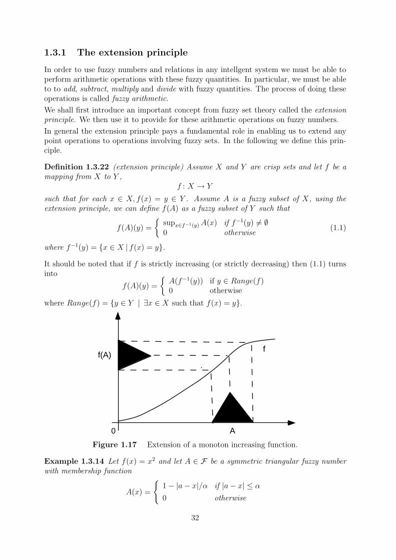
It should be noted that if f is strictly increasing (or strictly decreasing) then (1.1) turnsinto
f(A)(y) =
{A(f−1(y)) if y ∈ Range(f)0 otherwise
where Range(f) = {y ∈ Y | ∃x ∈ X such that f(x) = y}.
Figure 1.17 Extension of a monoton increasing function.
Example 1.3.14 Let f(x) = x2 and let A ∈ F be a symmetric triangular fuzzy numberwith membership function
A(x) =
{1− |a− x|/α if |a− x| ≤ α
0 otherwise
32
A
f(A)
1
1
f(x) = x2
A 2A1
a 2a
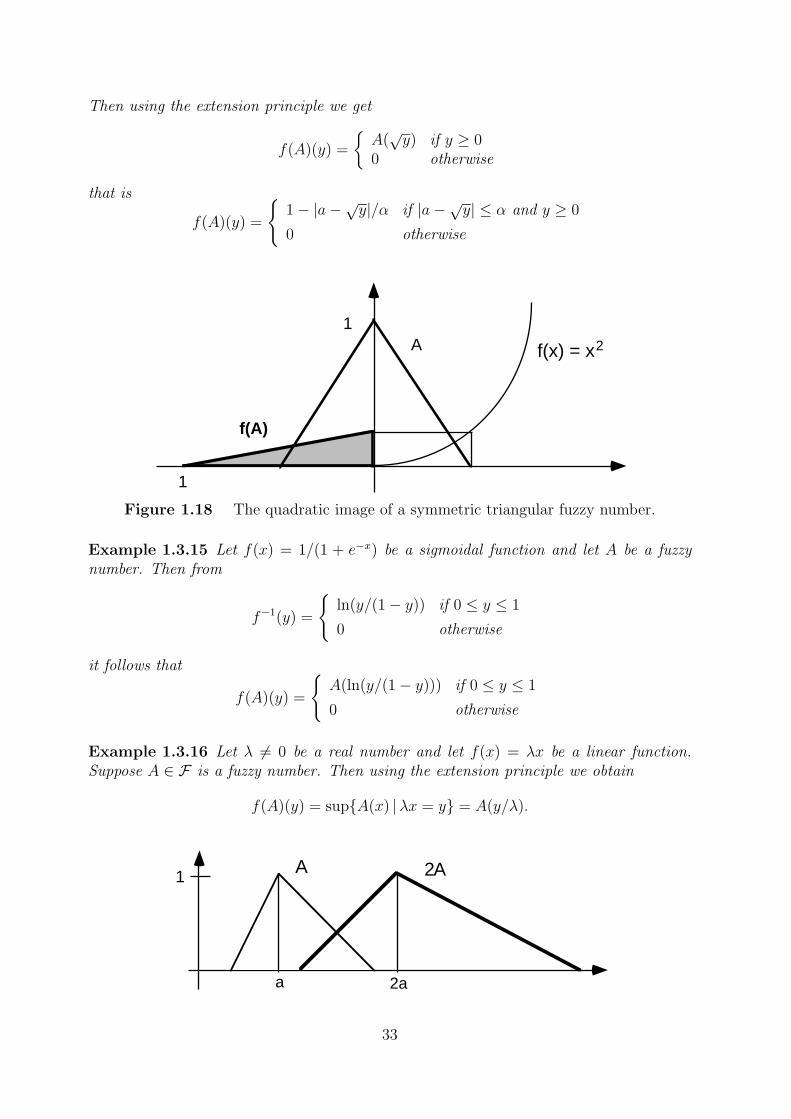
Then using the extension principle we get
f(A)(y) =
{A(√y) if y ≥ 0
0 otherwise
that is
f(A)(y) =
{1− |a−√y|/α if |a−√y| ≤ α and y ≥ 0
0 otherwise
Figure 1.18 The quadratic image of a symmetric triangular fuzzy number.
Example 1.3.15 Let f(x) = 1/(1 + e−x) be a sigmoidal function and let A be a fuzzynumber. Then from
f−1(y) =
{ln(y/(1− y)) if 0 ≤ y ≤ 1
0 otherwise
it follows that
f(A)(y) =
{A(ln(y/(1− y))) if 0 ≤ y ≤ 1
0 otherwise
Example 1.3.16 Let λ 6= 0 be a real number and let f(x) = λx be a linear function.Suppose A ∈ F is a fuzzy number. Then using the extension principle we obtain
f(A)(y) = sup{A(x) |λx = y} = A(y/λ).
33
1
A-A
a-a a+β-a- β a- α-a+ α
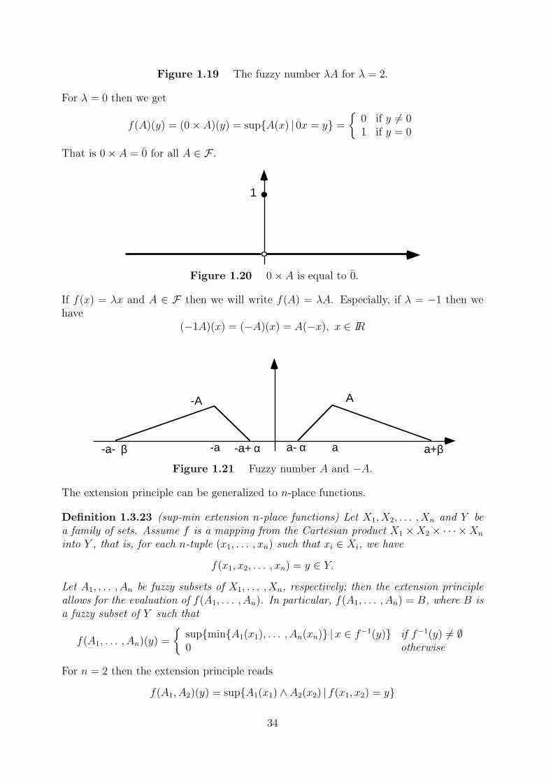
Figure 1.19 The fuzzy number λA for λ = 2.
For λ = 0 then we get
f(A)(y) = (0× A)(y) = sup{A(x) | 0x = y} =
{0 if y 6= 01 if y = 0
That is 0× A = 0 for all A ∈ F .
Figure 1.20 0× A is equal to 0.
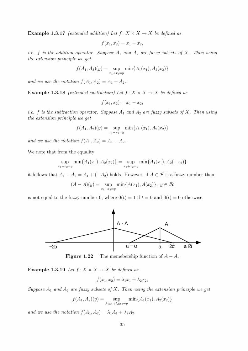
If f(x) = λx and A ∈ F then we will write f(A) = λA. Especially, if λ = −1 then wehave
(−1A)(x) = (−A)(x) = A(−x), x ∈ IR
Figure 1.21 Fuzzy number A and −A.
The extension principle can be generalized to n-place functions.
Definition 1.3.23 (sup-min extension n-place functions) Let X1, X2, . . . , Xn and Y bea family of sets. Assume f is a mapping from the Cartesian product X1 ×X2 × · · · ×Xn
into Y , that is, for each n-tuple (x1, . . . , xn) such that xi ∈ Xi, we have
f(x1, x2, . . . , xn) = y ∈ Y.
Let A1, . . . , An be fuzzy subsets of X1, . . . , Xn, respectively; then the extension principleallows for the evaluation of f(A1, . . . , An). In particular, f(A1, . . . , An) = B, where B isa fuzzy subset of Y such that
f(A1, . . . , An)(y) =
{sup{min{A1(x1), . . . , An(xn)} |x ∈ f−1(y)} if f−1(y) 6= ∅0 otherwise
For n = 2 then the extension principle reads
f(A1, A2)(y) = sup{A1(x1) ∧ A2(x2) | f(x1, x2) = y}
34
a
AA - A
2α−2α a + αa − α
Example 1.3.17 (extended addition) Let f : X ×X → X be defined as
f(x1, x2) = x1 + x2,
i.e. f is the addition operator. Suppose A1 and A2 are fuzzy subsets of X. Then usingthe extension principle we get
f(A1, A2)(y) = supx1+x2=y
min{A1(x1), A2(x2)}
and we use the notation f(A1, A2) = A1 + A2.
Example 1.3.18 (extended subtraction) Let f : X ×X → X be defined as
f(x1, x2) = x1 − x2,
i.e. f is the subtraction operator. Suppose A1 and A2 are fuzzy subsets of X. Then usingthe extension principle we get
f(A1, A2)(y) = supx1−x2=y
min{A1(x1), A2(x2)}
and we use the notation f(A1, A2) = A1 − A2.
We note that from the equality
supx1−x2=y
min{A1(x1), A2(x2)} = supx1+x2=y
min{A1(x1), A2(−x2)}
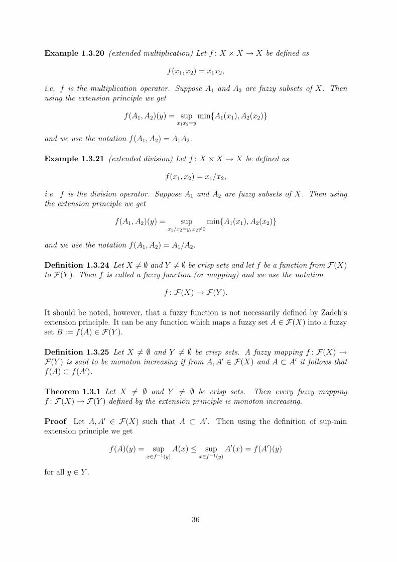
it follows that A1 − A2 = A1 + (−A2) holds. However, if A ∈ F is a fuzzy number then
(A− A)(y) = supx1−x2=y
min{A(x1), A(x2)}, y ∈ IR
is not equal to the fuzzy number 0, where 0(t) = 1 if t = 0 and 0(t) = 0 otherwise.
Figure 1.22 The memebership function of A− A.
Example 1.3.19 Let f : X ×X → X be defined as
f(x1, x2) = λ1x1 + λ2x2,
Suppose A1 and A2 are fuzzy subsets of X. Then using the extension principle we get
f(A1, A2)(y) = supλ1x1+λ2x2=y
min{A1(x1), A2(x2)}
and we use the notation f(A1, A2) = λ1A1 + λ2A2.
35
Example 1.3.20 (extended multiplication) Let f : X ×X → X be defined as
f(x1, x2) = x1x2,
i.e. f is the multiplication operator. Suppose A1 and A2 are fuzzy subsets of X. Thenusing the extension principle we get
f(A1, A2)(y) = supx1x2=y
min{A1(x1), A2(x2)}
and we use the notation f(A1, A2) = A1A2.
Example 1.3.21 (extended division) Let f : X ×X → X be defined as
f(x1, x2) = x1/x2,
i.e. f is the division operator. Suppose A1 and A2 are fuzzy subsets of X. Then usingthe extension principle we get
f(A1, A2)(y) = supx1/x2=y, x2 6=0
min{A1(x1), A2(x2)}
and we use the notation f(A1, A2) = A1/A2.
Definition 1.3.24 Let X 6= ∅ and Y 6= ∅ be crisp sets and let f be a function from F(X)to F(Y ). Then f is called a fuzzy function (or mapping) and we use the notation
f : F(X)→ F(Y ).
It should be noted, however, that a fuzzy function is not necessarily defined by Zadeh’sextension principle. It can be any function which maps a fuzzy set A ∈ F(X) into a fuzzyset B := f(A) ∈ F(Y ).
Definition 1.3.25 Let X 6= ∅ and Y 6= ∅ be crisp sets. A fuzzy mapping f : F(X) →F(Y ) is said to be monoton increasing if from A,A′ ∈ F(X) and A ⊂ A′ it follows thatf(A) ⊂ f(A′).
Theorem 1.3.1 Let X 6= ∅ and Y 6= ∅ be crisp sets. Then every fuzzy mappingf : F(X)→ F(Y ) defined by the extension principle is monoton increasing.
Proof Let A,A′ ∈ F(X) such that A ⊂ A′. Then using the definition of sup-minextension principle we get
f(A)(y) = supx∈f−1(y)
A(x) ≤ supx∈f−1(y)
A′(x) = f(A′)(y)
for all y ∈ Y .
36
Lemma 1.3.1 Let A,B ∈ F be fuzzy numbers and let f(A,B) = A + B be defined bysup-min extension principle. Then f is monoton increasing.
Proof Let A,A′, B,B′ ∈ F such that A ⊂ A′ and B ⊂ B′. Then using the definition ofsup-min extension principle we get
(A+B)(z) = supx+y=z
min{A(x), B(y)} ≤ supx+y=z
min{A′(x), B′(y)} = (A′ +B′)(z)
Which ends the proof.
The following lemma can be proved in a similar way.
Lemma 1.3.2 Let A,B ∈ F be fuzzy numbers, let λ1, λ2 be real numbers and let
f(A,B) = λ1A+ λ2B
be defined by sup-min extension principle. Then f is a monoton increasing fuzzy function.
Let A = (a1, a2, α1, α2)LR and B = (b1, b2, β1, β2)LR be fuzzy numbers of LR-type. Us-ing the (sup-min) extension principle we can verify the following rules for addition andsubtraction of fuzzy numbers of LR-type.
A+B = (a1 + b1, a2 + b2, α1 + β1, α2 + β2)LR
A−B = (a1 − b2, a2 − b1, α1 + β1, α2 + β2)LR
furthermore, if λ ∈ IR is a real number then λA can be represented as
λA =
{(λa1, λa2, α1, α2)LR if λ ≥ 0
(λa2, λa1, |λ|α2, |λ|α1)LR if λ < 0
In particular if A = (a1, a2, α1, α2) and B = (b1, b2, β1, β2) are fuzzy numbers of trapezoidalform then
A+B = (a1 + b1, a2 + b2, α1 + β1, α2 + β2)
A−B = (a1 − b2, a2 − b1, α1 + β2, α2 + β1).
If A = (a, α1, α2) and B = (b, β1, β2) are fuzzy numbers of triangular form then
A+B = (a+ b, α1 + β1, α2 + β2)
A−B = (a− b, α1 + β2, α2 + β1)
and if A = (a, α) and B = (b, β) are fuzzy numbers of symmetrical triangular form then
A+B = (a+ b, α + β)
A−B = (a− b, α + β)
λA = (λa, |λ|α).
The above results can be generalized to linear combinations of fuzzy numbers.
37
a ba + b
A A + B B
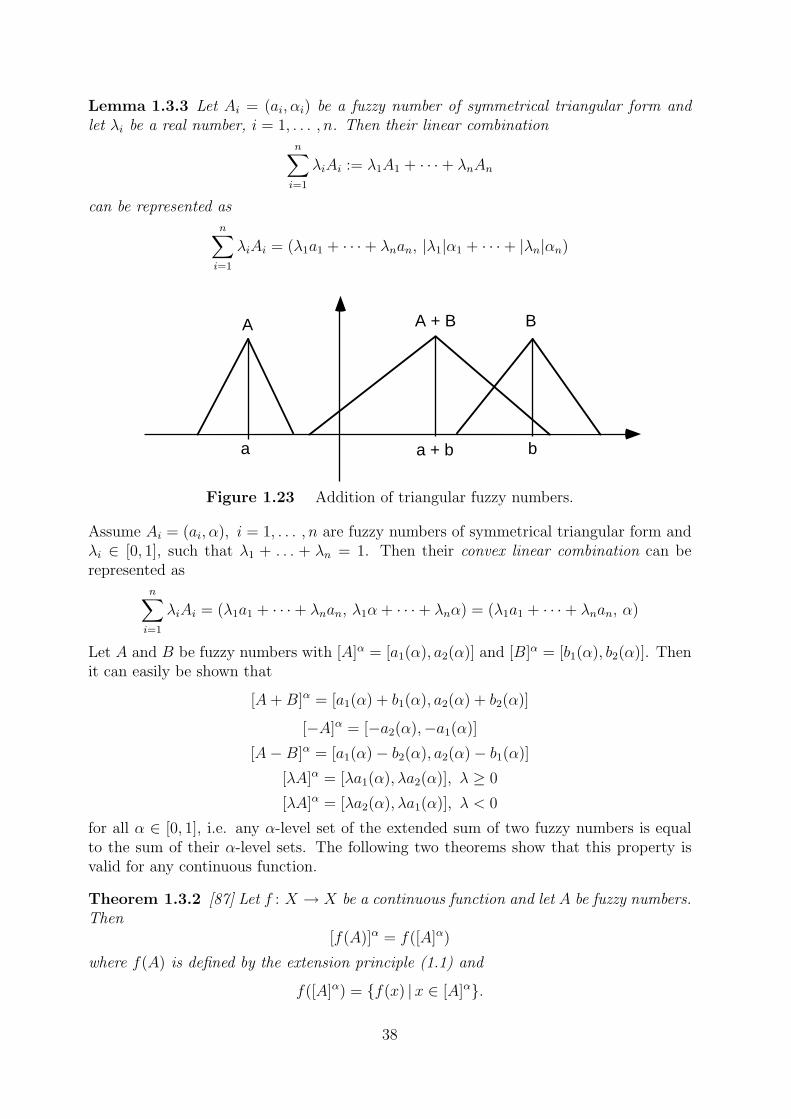
Lemma 1.3.3 Let Ai = (ai, αi) be a fuzzy number of symmetrical triangular form andlet λi be a real number, i = 1, . . . , n. Then their linear combination
n∑i=1
λiAi := λ1A1 + · · ·+ λnAn
can be represented asn∑i=1
λiAi = (λ1a1 + · · ·+ λnan, |λ1|α1 + · · ·+ |λn|αn)
Figure 1.23 Addition of triangular fuzzy numbers.
Assume Ai = (ai, α), i = 1, . . . , n are fuzzy numbers of symmetrical triangular form andλi ∈ [0, 1], such that λ1 + . . . + λn = 1. Then their convex linear combination can berepresented as
n∑i=1
λiAi = (λ1a1 + · · ·+ λnan, λ1α + · · ·+ λnα) = (λ1a1 + · · ·+ λnan, α)
Let A and B be fuzzy numbers with [A]α = [a1(α), a2(α)] and [B]α = [b1(α), b2(α)]. Thenit can easily be shown that
[A+B]α = [a1(α) + b1(α), a2(α) + b2(α)]
[−A]α = [−a2(α),−a1(α)]
[A−B]α = [a1(α)− b2(α), a2(α)− b1(α)]
[λA]α = [λa1(α), λa2(α)], λ ≥ 0
[λA]α = [λa2(α), λa1(α)], λ < 0
for all α ∈ [0, 1], i.e. any α-level set of the extended sum of two fuzzy numbers is equalto the sum of their α-level sets. The following two theorems show that this property isvalid for any continuous function.
Theorem 1.3.2 [87] Let f : X → X be a continuous function and let A be fuzzy numbers.Then
[f(A)]α = f([A]α)
where f(A) is defined by the extension principle (1.1) and
f([A]α) = {f(x) |x ∈ [A]α}.
38
A B
fuzzy max
If [A]α = [a1(α), a2(α)] and f is monoton increasing then from the above theorem we get
[f(A)]α = f([A]α) = f([a1(α), a2(α)]) = [f(a1(α)), f(a2(α))].
Theorem 1.3.3 [87] Let f : X × X → X be a continuous function and let A and B befuzzy numbers. Then
[f(A,B)]α = f([A]α, [B]α)
wheref([A]α, [B]α) = {f(x1, x2) |x1 ∈ [A]α, x2 ∈ [B]α}.
Let f(x, y) = xy and let [A]α = [a1(α), a2(α)] and [B]α = [b1(α), b2(α)] be two fuzzynumbers. Applying Theorem 1.3.3 we get
[f(A,B)]α = f([A]α, [B]α) = [A]α[B]α.
However the equation
[AB]α = [A]α[B]α = [a1(α)b1(α), a2(α)b2(α)]
holds if and only if A and B are both nonnegative, i.e. A(x) = B(x) = 0 for x ≤ 0.
If B is nonnegative then we have
[A]α[B]α = [min{a1(α)b1(α), a1(α)b2(α)},max{a2(α)b1(α), a2(α)b2(α)]
In general case we obtain a very complicated expression for the α level sets of the productAB
[A]α[B]α = [min{a1(α)b1(α), a1(α)b2(α), a2(α)b1(α), a2(α)b2(α)},max{a1(α)b1(α), a1(α)b2(α), a2(α)b1(α), a2(α)b2(α)]
The above properties of extended operations addition, subtraction and multiplication byscalar of fuzzy fuzzy numbers of type LR are often used in fuzzy neural networks.
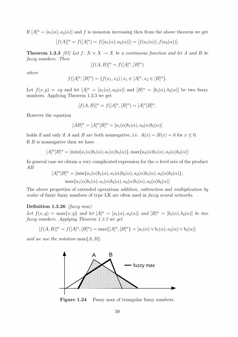
Definition 1.3.26 (fuzzy max)
Let f(x, y) = max{x, y} and let [A]α = [a1(α), a2(α)] and [B]α = [b1(α), b2(α)] be twofuzzy numbers. Applying Theorem 1.3.3 we get
[f(A,B)]α = f([A]α, [B]α) = max{[A]α, [B]α} = [a1(α) ∨ b1(α), a2(α) ∨ b2(α)]
and we use the notation max{A,B}.
Figure 1.24 Fuzzy max of triangular fuzzy numbers.
39
A B
fuzzy min
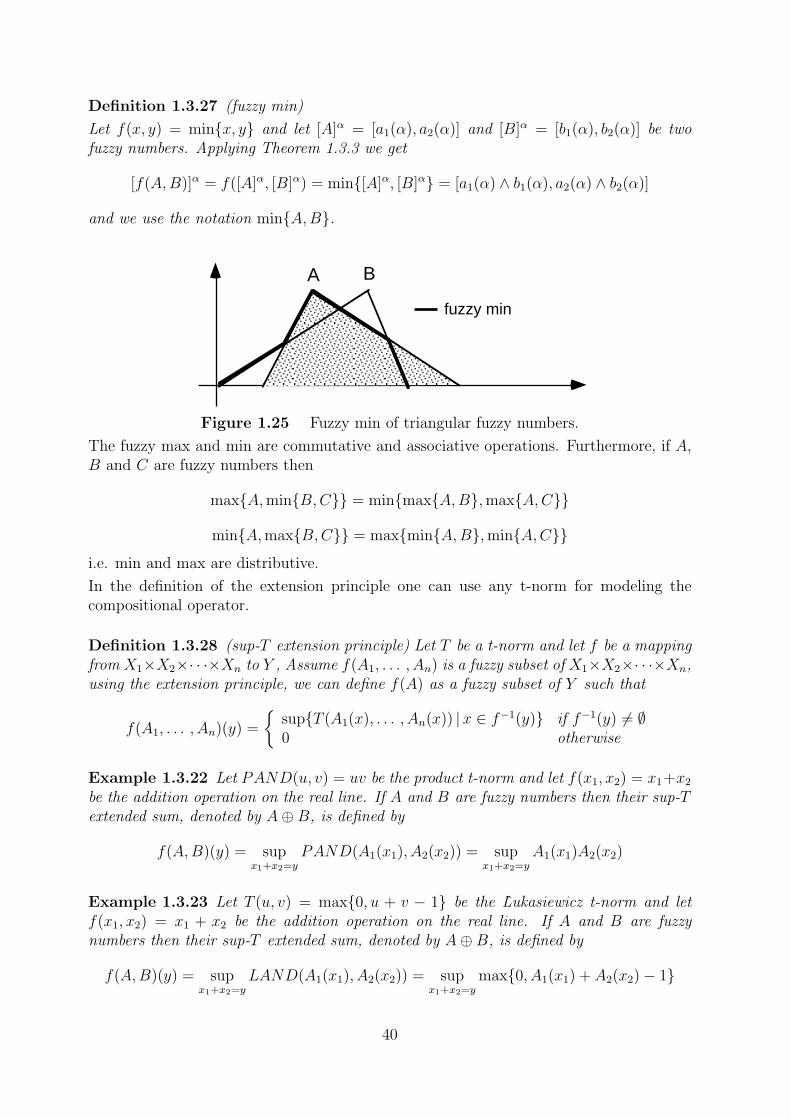
Definition 1.3.27 (fuzzy min)
Let f(x, y) = min{x, y} and let [A]α = [a1(α), a2(α)] and [B]α = [b1(α), b2(α)] be twofuzzy numbers. Applying Theorem 1.3.3 we get
[f(A,B)]α = f([A]α, [B]α) = min{[A]α, [B]α} = [a1(α) ∧ b1(α), a2(α) ∧ b2(α)]
and we use the notation min{A,B}.
Figure 1.25 Fuzzy min of triangular fuzzy numbers.
The fuzzy max and min are commutative and associative operations. Furthermore, if A,B and C are fuzzy numbers then
max{A,min{B,C}} = min{max{A,B},max{A,C}}
min{A,max{B,C}} = max{min{A,B},min{A,C}}i.e. min and max are distributive.
In the definition of the extension principle one can use any t-norm for modeling thecompositional operator.
Definition 1.3.28 (sup-T extension principle) Let T be a t-norm and let f be a mappingfrom X1×X2×· · ·×Xn to Y , Assume f(A1, . . . , An) is a fuzzy subset of X1×X2×· · ·×Xn,using the extension principle, we can define f(A) as a fuzzy subset of Y such that
f(A1, . . . , An)(y) =
{sup{T (A1(x), . . . , An(x)) | x ∈ f−1(y)} if f−1(y) 6= ∅0 otherwise
Example 1.3.22 Let PAND(u, v) = uv be the product t-norm and let f(x1, x2) = x1+x2
be the addition operation on the real line. If A and B are fuzzy numbers then their sup-Textended sum, denoted by A⊕B, is defined by
f(A,B)(y) = supx1+x2=y
PAND(A1(x1), A2(x2)) = supx1+x2=y
A1(x1)A2(x2)
Example 1.3.23 Let T (u, v) = max{0, u + v − 1} be the ÃLukasiewicz t-norm and letf(x1, x2) = x1 + x2 be the addition operation on the real line. If A and B are fuzzynumbers then their sup-T extended sum, denoted by A⊕B, is defined by
f(A,B)(y) = supx1+x2=y
LAND(A1(x1), A2(x2)) = supx1+x2=y
max{0, A1(x1) + A2(x2)− 1}
40

The reader can find some results on t-norm-based operations on fuzzy numbers in [45, 46,52].
Exercise 1.3.1 Let A1 = (a1, α) and A2 = (a2, α) be fuzzy numbers of symmetric trian-gular form. Compute analytically the membership function of their product-sum, A1⊕A2,defined by
(A1 ⊕ A2)(y) = supx1+x2=y
PAND(A1(x1), A2(x2)) = supx1+x2=y
A1(x1)A2(x2).
41
A B
a ba- α a+α b+αb- α
1D(A,B) = |a-b|
A B1C(A,B) = 1
1.3.2 Metrics for fuzzy numbers
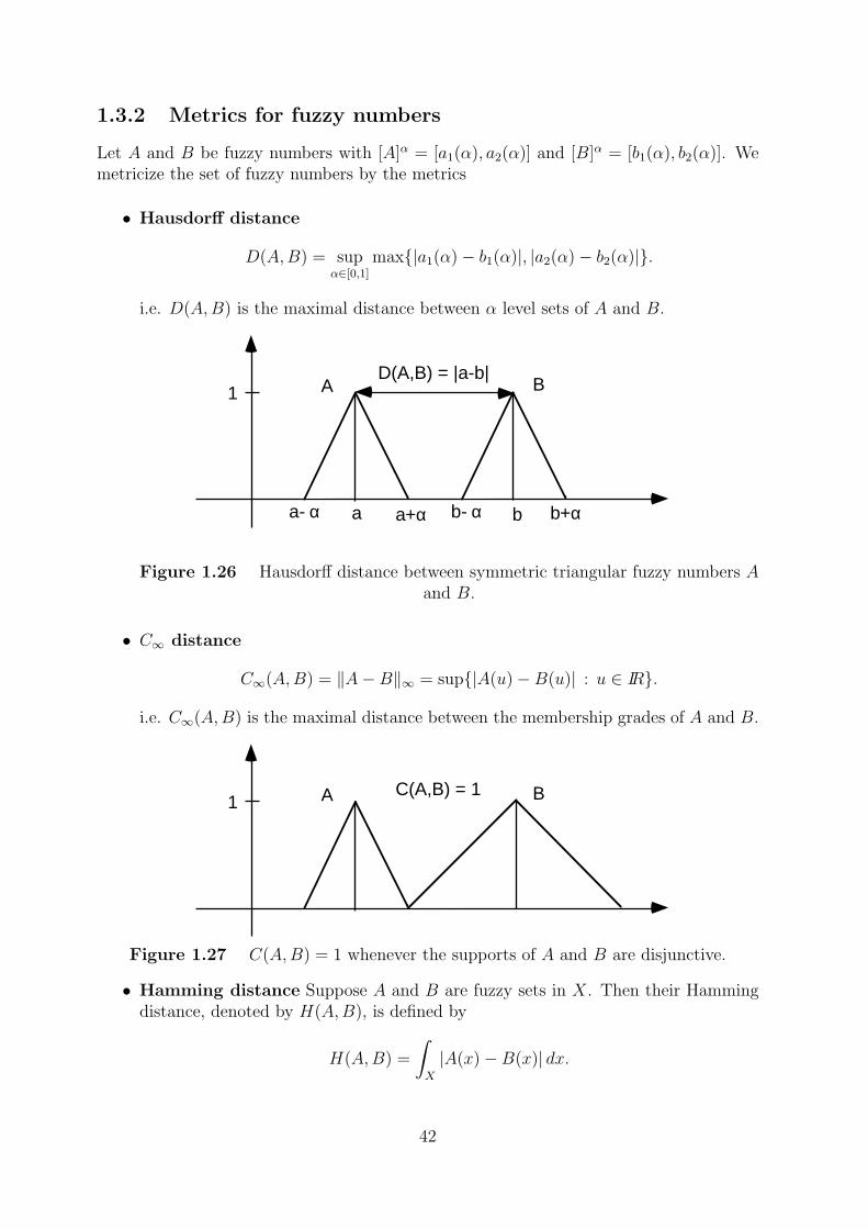
Let A and B be fuzzy numbers with [A]α = [a1(α), a2(α)] and [B]α = [b1(α), b2(α)]. Wemetricize the set of fuzzy numbers by the metrics
• Hausdorff distance
D(A,B) = supα∈[0,1]
max{|a1(α)− b1(α)|, |a2(α)− b2(α)|}.
i.e. D(A,B) is the maximal distance between α level sets of A and B.
Figure 1.26 Hausdorff distance between symmetric triangular fuzzy numbers Aand B.
• C∞ distance
C∞(A,B) = ‖A−B‖∞ = sup{|A(u)−B(u)| : u ∈ IR}.
i.e. C∞(A,B) is the maximal distance between the membership grades of A and B.
Figure 1.27 C(A,B) = 1 whenever the supports of A and B are disjunctive.
• Hamming distance Suppose A and B are fuzzy sets in X. Then their Hammingdistance, denoted by H(A,B), is defined by
H(A,B) =
∫X
|A(x)−B(x)| dx.
42
• Discrete Hamming distance Suppose A and B are discrete fuzzy sets
A = µ1/x1 + . . .+ µn/xn, B = ν1/x1 + . . .+ νn/xn
Then their Hamming distance is defined by
H(A,B) =n∑j=1
|µj − νj|.
It should be noted that D(A,B) is a better measure of similarity than C∞(A,B), becauseC∞(A,B) ≤ 1 holds even though the supports of A and B are very far from each other.
Definition 1.3.29 Let f be a fuzzy function from F to F . Then f is said to be continuousin metric D if ∀ε > 0 there exists δ > 0 such that if
D(A,B) ≤ δ
thenD(f(A), f(B)) ≤ ε
In a similar way we can define the continuity of fuzzy functions in metric C∞.
Definition 1.3.30 Let f be a fuzzy function from F(IR) to F(IR). Then f is said to becontinuous in metric C∞ if ∀ε > 0 there exists δ > 0 such that if
C∞(A,B) ≤ δ
thenC∞(f(A), f(B)) ≤ ε.
We note that in the definition of continuity in metric C∞ the domain and the range of fcan be the family of all fuzzy subsets of the real line, while in the case of continuity inmetric D the the domain and the range of f is the set of fuzzy numbers.
Exercise 1.3.2 Let f(x) = sinx and let A = (a, α) be a fuzzy number of symmetrictriangular form. Calculate the membership function of the fuzzy set f(A).
Exercise 1.3.3 Let B1 = (b1, β1) and B2 = (b2, β2) be fuzzy number of symmetric trian-gular form. Calculate the α-level set of their product B1B2.
Exercise 1.3.4 Let B1 = (b1, β1) and B2 = (b2, β2) be fuzzy number of symmetric trian-gular form. Calculate the α-level set of their fuzzy max max{B1, B2}.
Exercise 1.3.5 Let B1 = (b1, β1) and B2 = (b2, β2) be fuzzy number of symmetric trian-gular form. Calculate the α-level set of their fuzzy min min{B1, B2}.
Exercise 1.3.6 Let A = (a, α) and B = (b, β) be fuzzy numbers of symmetrical triangularform. Calculate the distances D(A,B), H(A,B) and C∞(A,B) as a function of a, b, αand β.
43
Exercise 1.3.7 Let A = (a, α1, α2) and B = (b, β1, β2) be fuzzy numbers of triangularform. Calculate the distances D(A,B), H(A,B) and C∞(A,B) as a function of a, b, α1,α2, β1 and β2.
Exercise 1.3.8 Let A = (a1, a2, α1, α2) and B = (b1, b2, β1, β2) be fuzzy numbers of trape-zoidal form. Calculate the distances D(A,B), H(A,B) and C∞(A,B).
Exercise 1.3.9 Let A = (a1, a2, α1, α2)LR and B = (b1, b2, β1, β2)LR be fuzzy numbers oftype LR. Calculate the distances D(A,B), H(A,B) and C∞(A,B).
Exercise 1.3.10 Let A and B be discrete fuzzy subsets of X = {−2,−1, 0, 1, 2, 3, 4}.
A = 0.7/− 2 + 0.4/− 1 + 0.6/0 + 1.0/1 + 0.6/2 + 0.3/3 + 0.4/4
B = 0.1/− 2 + 0.2/− 1 + 0.9/0 + 1.0/1 + 1.0/2 + 0.3/3 + 0.2/4
Calculate the Hamming distance between A and B.
1.3.3 Fuzzy implications
Let p = ”x is in A” and q = ”y is in B” be crisp propositions, where A and B are crisp setsfor the moment. The implication p→ q is interpreted as ¬(p∧¬q). The full interpretationof the material implication p→ q is that the degree of truth of p→ q quantifies to whatextend q is at least as true as p, i.e.
τ(p→ q) =
{1 if τ(p) ≤ τ(q)0 otherwise
where τ(.) denotes the truth value of a proposition.
τ(p) τ(q) τ(p→ q)1 1 10 1 10 0 11 0 0
Table 1.3 Truth table for the material implication.
Example 1.3.24 Let p = ”x is bigger than 10” and let q = ”x is bigger than 9”. It iseasy to see that p → q is true, because it can never happen that x is bigger than 10 andat the same time x is not bigger than 9.
Consider the implication statement: if ”pressure is high” then ”volume is small”. Themembership function of the fuzzy set A = ”big pressure”,
A(u) =
1 if u ≥ 5
1− (5− u)/4 if 1 ≤ u ≤ 5
0 otherwise
can be interpreted as
44
1 5 x 1 5 y
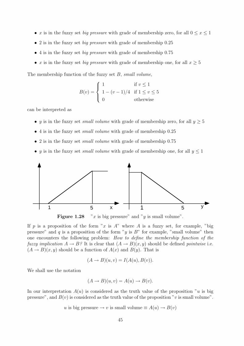
• x is in the fuzzy set big pressure with grade of membership zero, for all 0 ≤ x ≤ 1
• 2 is in the fuzzy set big pressure with grade of membership 0.25
• 4 is in the fuzzy set big pressure with grade of membership 0.75
• x is in the fuzzy set big pressure with grade of membership one, for all x ≥ 5
The membership function of the fuzzy set B, small volume,
B(v) =
1 if v ≤ 1
1− (v − 1)/4 if 1 ≤ v ≤ 5
0 otherwise
can be interpreted as
• y is in the fuzzy set small volume with grade of membership zero, for all y ≥ 5
• 4 is in the fuzzy set small volume with grade of membership 0.25
• 2 is in the fuzzy set small volume with grade of membership 0.75
• y is in the fuzzy set small volume with grade of membership one, for all y ≤ 1
Figure 1.28 ”x is big pressure” and ”y is small volume”.
If p is a proposition of the form ”x is A” where A is a fuzzy set, for example, ”bigpressure” and q is a proposition of the form ”y is B” for example, ”small volume” thenone encounters the following problem: How to define the membership function of thefuzzy implication A→ B? It is clear that (A→ B)(x, y) should be defined pointwise i.e.(A→ B)(x, y) should be a function of A(x) and B(y). That is
(A→ B)(u, v) = I(A(u), B(v)).
We shall use the notation
(A→ B)(u, v) = A(u)→ B(v).
In our interpretation A(u) is considered as the truth value of the proposition ”u is bigpressure”, and B(v) is considered as the truth value of the proposition ”v is small volume”.
u is big pressure→ v is small volume ≡ A(u)→ B(v)
45
One possible extension of material implication to implications with intermediate truthvalues is
A(u)→ B(v) =
{1 if A(u) ≤ B(v)0 otherwise
This implication operator is called Standard Strict.
”4 is big pressure”→ ”1 is small volume” = A(4)→ B(1) = 0.75→ 1 = 1
However, it is easy to see that this fuzzy implication operator is not appropriate forreal-life applications. Namely, let A(u) = 0.8 and B(v) = 0.8. Then we have
A(u)→ B(v) = 0.8→ 0.8 = 1
Let us suppose that there is a small error of measurement or small rounding error ofdigital computation in the value of B(v), and instead 0.8 we have to proceed with 0.7999.Then from the definition of Standard Strict implication operator it follows that
A(u)→ B(v) = 0.8→ 0.7999 = 0
This example shows that small changes in the input can cause a big deviation in theoutput, i.e. our system is very sensitive to rounding errors of digital computation andsmall errors of measurement.
A smoother extension of material implication operator can be derived from the equation
X → Y = sup{Z|X ∩ Z ⊂ Y }
where X, Y and Z are classical sets.
Using the above principle we can define the following fuzzy implication operator
A(u)→ B(v) = sup{z|min{A(u), z} ≤ B(v)}
that is,
A(u)→ B(v) =
{1 if A(u) ≤ B(v)B(v) otherwise
This operator is called Godel implication. Using the definitions of negation and union offuzzy subsets the material implication p→ q = ¬p ∨ q can be extended by
A(u)→ B(v) = max{1− A(u), B(v)}
This operator is called Kleene-Dienes implication.
In many practical applications one uses Mamdani’s implication operator to model causalrelationship between fuzzy variables. This operator simply takes the minimum of truthvalues of fuzzy predicates
A(u)→ B(v) = min{A(u), B(v)}
It is easy to see this is not a correct extension of material implications, because 0 → 0yields zero. However, in knowledge-based systems, we are usually not interested in rules,in which the antecedent part is false.
There are three important classes of fuzzy implication operators:
46
• S-implications: defined by
x→ y = S(n(x), y)
where S is a t-conorm and n is a negation on [0, 1]. These implications arise fromthe Boolean formalism p→ q = ¬p∨ q. Typical examples of S-implications are theÃLukasiewicz and Kleene-Dienes implications.
• R-implications: obtained by residuation of continuous t-norm T , i.e.
x→ y = sup{z ∈ [0, 1] |T (x, z) ≤ y}
These implications arise from the Intutionistic Logic formalism. Typical examplesof R-implications are the Godel and Gaines implications.
• t-norm implications: if T is a t-norm then
x→ y = T (x, y)
Although these implications do not verify the properties of material implicationthey are used as model of implication in many applications of fuzzy logic. Typicalexamples of t-norm implications are the Mamdani (x→ y = min{x, y}) and Larsen(x→ y = xy) implications.
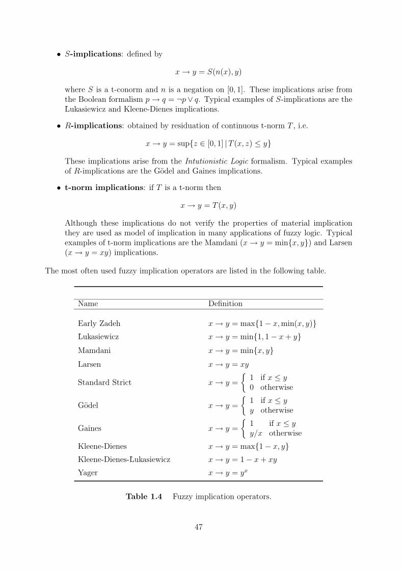
The most often used fuzzy implication operators are listed in the following table.
Name Definition
Early Zadeh x→ y = max{1− x,min(x, y)}ÃLukasiewicz x→ y = min{1, 1− x+ y}Mamdani x→ y = min{x, y}Larsen x→ y = xy
Standard Strict x→ y =
{1 if x ≤ y0 otherwise
Godel x→ y =
{1 if x ≤ yy otherwise
Gaines x→ y =
{1 if x ≤ yy/x otherwise
Kleene-Dienes x→ y = max{1− x, y}Kleene-Dienes-ÃLukasiewicz x→ y = 1− x+ xy
Yager x→ y = yx
Table 1.4 Fuzzy implication operators.
47
speed
slow medium fast
40 55 70
1
1.3.4 Linguistic variables
The use of fuzzy sets provides a basis for a systematic way for the manipulation of vagueand imprecise concepts. In particular, we can employ fuzzy sets to represent linguisticvariables. A linguistic variable can be regarded either as a variable whose value is a fuzzynumber or as a variable whose values are defined in linguistic terms.
Definition 1.3.31 (linguistic variable) A linguistic variable is characterized by a quin-tuple
(x, T (x), U,G,M)
in which
• x is the name of variable;
• T (x) is the term set of x, that is, the set of names of linguistic values of x with eachvalue being a fuzzy number defined on U ;
• G is a syntactic rule for generating the names of values of x;
• and M is a semantic rule for associating with each value its meaning.
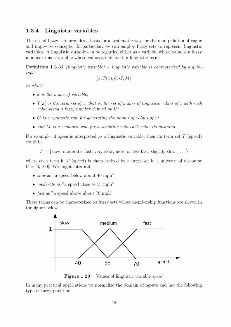
For example, if speed is interpreted as a linguistic variable, then its term set T (speed)could be
T = {slow, moderate, fast, very slow, more or less fast, sligthly slow, . . . }
where each term in T (speed) is characterized by a fuzzy set in a universe of discourseU = [0, 100]. We might interpret
• slow as ”a speed below about 40 mph”
• moderate as ”a speed close to 55 mph”
• fast as ”a speed above about 70 mph”
These terms can be characterized as fuzzy sets whose membership functions are shown inthe figure below.
Figure 1.29 Values of linguistic variable speed.
In many practical applications we normalize the domain of inputs and use the followingtype of fuzzy partition
48
NB PBPMPSZENSNM
-1 1
old
very old
30 60
30 60
old
more or less old
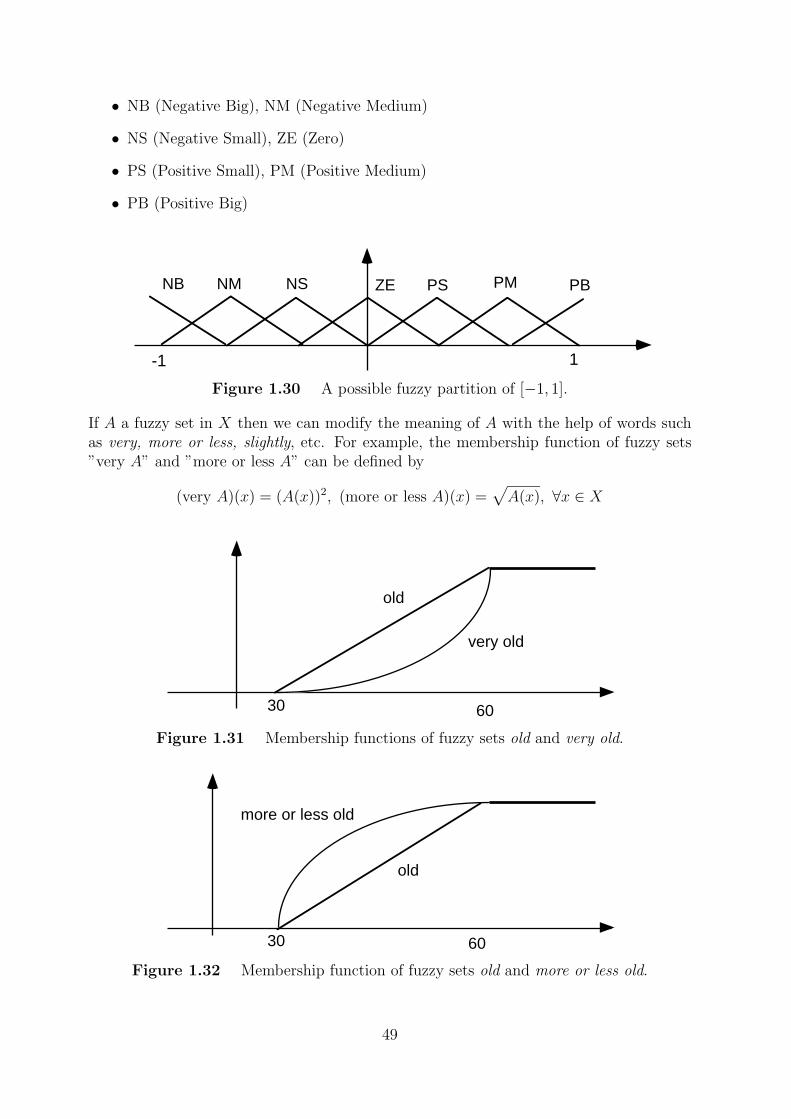
• NB (Negative Big), NM (Negative Medium)
• NS (Negative Small), ZE (Zero)
• PS (Positive Small), PM (Positive Medium)
• PB (Positive Big)
Figure 1.30 A possible fuzzy partition of [−1, 1].
If A a fuzzy set in X then we can modify the meaning of A with the help of words suchas very, more or less, slightly, etc. For example, the membership function of fuzzy sets”very A” and ”more or less A” can be defined by
(very A)(x) = (A(x))2, (more or less A)(x) =√A(x), ∀x ∈ X
Figure 1.31 Membership functions of fuzzy sets old and very old.
Figure 1.32 Membership function of fuzzy sets old and more or less old.
49
x
y
y=f(x)
y=f(x’)
x=x'
1.4 The theory of approximate reasoning
In 1979 Zadeh introduced the theory of approximate reasoning [118]. This theory providesa powerful framework for reasoning in the face of imprecise and uncertain information.Central to this theory is the representation of propositions as statements assigning fuzzysets as values to variables.
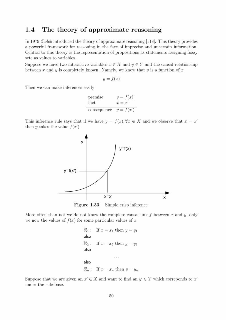
Suppose we have two interactive variables x ∈ X and y ∈ Y and the causal relationshipbetween x and y is completely known. Namely, we know that y is a function of x
y = f(x)
Then we can make inferences easily
premise y = f(x)fact x = x′
consequence y = f(x′)
This inference rule says that if we have y = f(x), ∀x ∈ X and we observe that x = x′
then y takes the value f(x′).
Figure 1.33 Simple crisp inference.
More often than not we do not know the complete causal link f between x and y, onlywe now the values of f(x) for some particular values of x
<1 : If x = x1 then y = y1
also
<2 : If x = x2 then y = y2
also
. . .also
<n : If x = xn then y = yn
Suppose that we are given an x′ ∈ X and want to find an y′ ∈ Y which correponds to x′
under the rule-base.
50
<1 : If x = x1 then y = y1
also
<2 : If x = x2 then y = y2
also
. . . . . .also
<n : If x = xn then y = ynfact: x = x′
consequence: y = y′
This problem is frequently quoted as interpolation.
Let x and y be linguistic variables, e.g. ”x is high” and ”y is small”. The basic problemof approximate reasoning is to find the membership function of the consequence C fromthe rule-base {<1, . . . ,<n} and the fact A.
<1 : if x is A1 then y is C1,
<2 : if x is A2 then y is C2,
· · · · · · · · · · · ·<n : if x is An then y is Cn
fact: x is A
consequence: y is C
In [118] Zadeh introduces a number of translation rules which allow us to represent somecommon linguistic statements in terms of propositions in our language. In the followingwe describe some of these translation rules.
Definition 1.4.1 Entailment rule:
x is A
A ⊂ B
x is B
Mary is very young
very young ⊂ young
Mary is young
Definition 1.4.2 Conjuction rule:
x is A
x is B
x is A ∩B
pressure is not very high
pressure is not very low
pressure is not very high and not very low
Definition 1.4.3 Disjunction rule:
x is A
or x is B
x is A ∪B
pressure is not very high vspace4ptor pressure is not very low
pressure is not very high or not very low
51
Definition 1.4.4 Projection rule:
(x, y) have relation R
x is ΠX(R)
(x, y) have relation R
y is ΠY (R)
(x, y) is close to (3, 2)
x is close to 3
(x, y) is close to (3, 2)
y is close to 2
Definition 1.4.5 Negation rule:
not (x is A)
x is ¬Anot (x is high)
x is not high
In fuzzy logic and approximate reasoning, the most important fuzzy implication inferencerule is the Generalized Modus Ponens (GMP). The classical Modus Ponens inference rulesays:
premise if p then qfact p
consequence q
This inference rule can be interpreted as: If p is true and p→ q is true then q is true.
The fuzzy implication inference is based on the compositional rule of inference for ap-proximate reasoning suggested by Zadeh [115].
Definition 1.4.6 (compositional rule of inference)
premise if x is A then y is Bfact x is A′
consequence: y is B′
where the consequence B′ is determined as a composition of the fact and the fuzzy impli-cation operator
B′ = A′ ◦ (A→ B)
that is,B′(v) = sup
u∈Umin{A′(u), (A→ B)(u, v)}, v ∈ V.
The consequence B′ is nothing else but the shadow of A→ B on A′.
The Generalized Modus Ponens, which reduces to calssical modus ponens when A′ = Aand B′ = B, is closely related to the forward data-driven inference which is particularlyuseful in the Fuzzy Logic Control.
In many practical cases instead of sup-min composition we use sup-T composition, whereT is a t-norm.
52
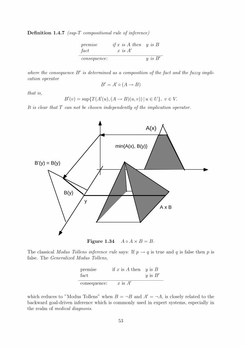
yA x B
A(x)
min{A(x), B(y)}
B'(y) = B(y)
B(y)
Definition 1.4.7 (sup-T compositional rule of inference)
premise if x is A then y is Bfact x is A′
consequence: y is B′
where the consequence B′ is determined as a composition of the fact and the fuzzy impli-cation operator
B′ = A′ ◦ (A→ B)
that is,B′(v) = sup{T (A′(u), (A→ B)(u, v)) |u ∈ U}, v ∈ V.
It is clear that T can not be chosen independently of the implication operator.
Figure 1.34 A ◦ A×B = B.
The classical Modus Tollens inference rule says: If p → q is true and q is false then p isfalse. The Generalized Modus Tollens,
premise if x is A then y is Bfact y is B′
consequence: x is A′
which reduces to ”Modus Tollens” when B = ¬B and A′ = ¬A, is closely related to thebackward goal-driven inference which is commonly used in expert systems, especially inthe realm of medical diagnosis.
53
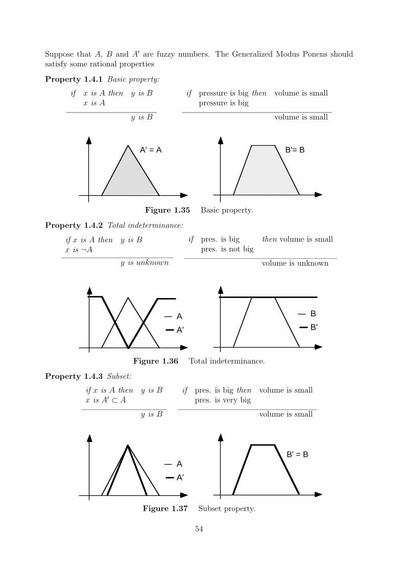
A' = A B'= B
B
B'A
A'
A
A'
B' = B
Suppose that A, B and A′ are fuzzy numbers. The Generalized Modus Ponens shouldsatisfy some rational properties
Property 1.4.1 Basic property:
if x is A then y is Bx is A
y is B
if pressure is big then volume is smallpressure is big
volume is small
Figure 1.35 Basic property.
Property 1.4.2 Total indeterminance:
if x is A then y is Bx is ¬A
y is unknown
if pres. is big then volume is smallpres. is not big
volume is unknown
Figure 1.36 Total indeterminance.
Property 1.4.3 Subset:
if x is A then y is Bx is A′ ⊂ A
y is B
if pres. is big then volume is smallpres. is very big
volume is small
Figure 1.37 Subset property.
54
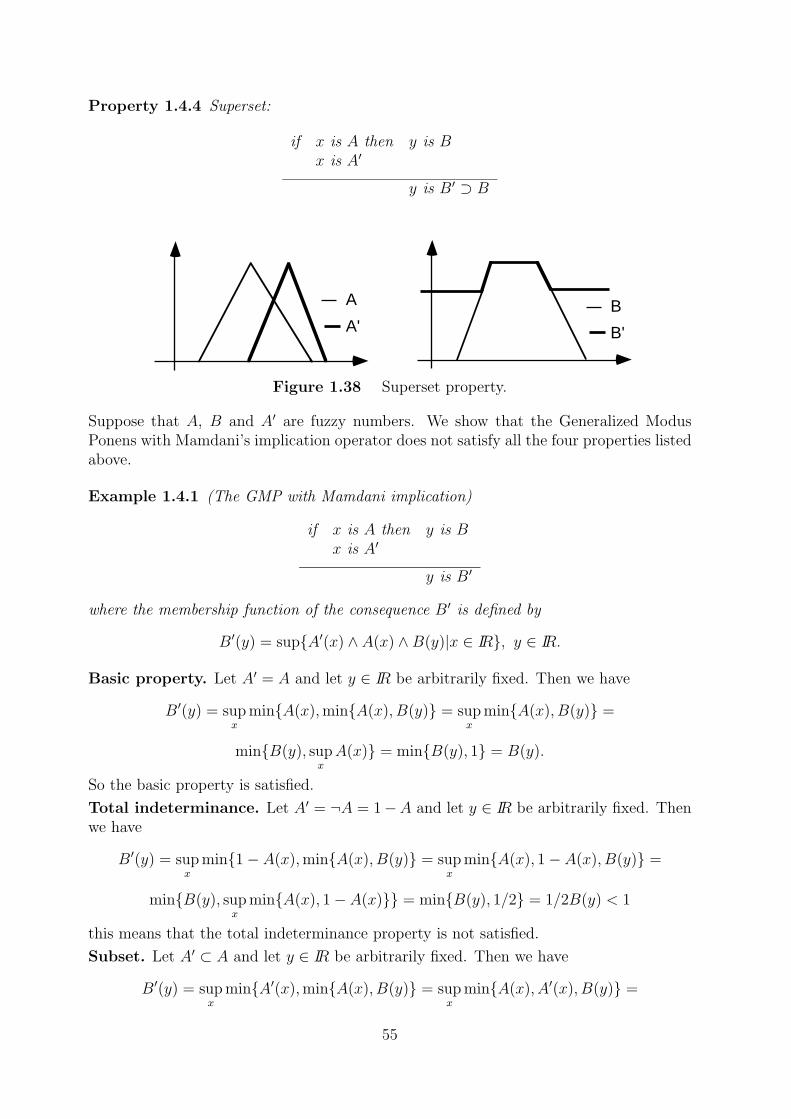
A
A'B
B'
Property 1.4.4 Superset:
if x is A then y is Bx is A′
y is B′ ⊃ B
Figure 1.38 Superset property.
Suppose that A, B and A′ are fuzzy numbers. We show that the Generalized ModusPonens with Mamdani’s implication operator does not satisfy all the four properties listedabove.
Example 1.4.1 (The GMP with Mamdani implication)
if x is A then y is Bx is A′
y is B′
where the membership function of the consequence B′ is defined by
B′(y) = sup{A′(x) ∧ A(x) ∧B(y)|x ∈ IR}, y ∈ IR.
Basic property. Let A′ = A and let y ∈ IR be arbitrarily fixed. Then we have
B′(y) = supx
min{A(x),min{A(x), B(y)} = supx
min{A(x), B(y)} =
min{B(y), supxA(x)} = min{B(y), 1} = B(y).
So the basic property is satisfied.
Total indeterminance. Let A′ = ¬A = 1−A and let y ∈ IR be arbitrarily fixed. Thenwe have
B′(y) = supx
min{1− A(x),min{A(x), B(y)} = supx
min{A(x), 1− A(x), B(y)} =
min{B(y), supx
min{A(x), 1− A(x)}} = min{B(y), 1/2} = 1/2B(y) < 1
this means that the total indeterminance property is not satisfied.
Subset. Let A′ ⊂ A and let y ∈ IR be arbitrarily fixed. Then we have
B′(y) = supx
min{A′(x),min{A(x), B(y)} = supx
min{A(x), A′(x), B(y)} =
55
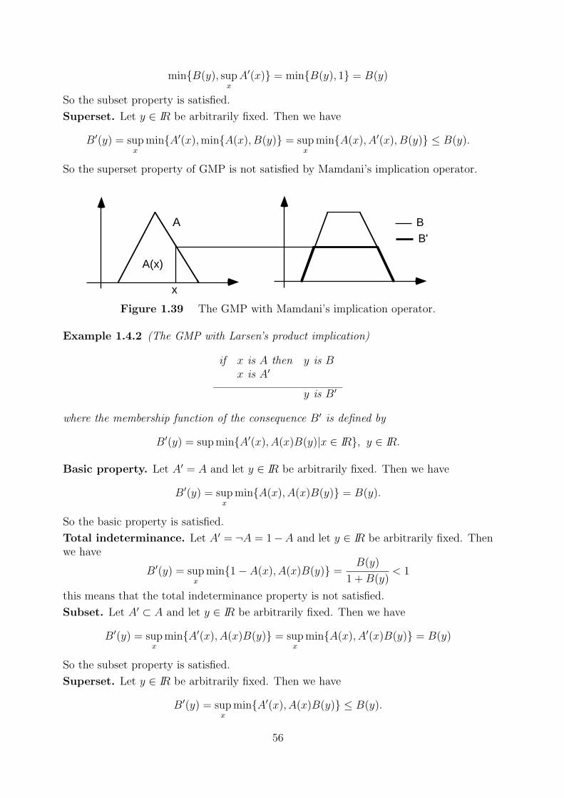
A B
x
A(x)
B'
min{B(y), supxA′(x)} = min{B(y), 1} = B(y)
So the subset property is satisfied.
Superset. Let y ∈ IR be arbitrarily fixed. Then we have
B′(y) = supx
min{A′(x),min{A(x), B(y)} = supx
min{A(x), A′(x), B(y)} ≤ B(y).
So the superset property of GMP is not satisfied by Mamdani’s implication operator.
Figure 1.39 The GMP with Mamdani’s implication operator.
Example 1.4.2 (The GMP with Larsen’s product implication)
if x is A then y is Bx is A′
y is B′
where the membership function of the consequence B′ is defined by
B′(y) = sup min{A′(x), A(x)B(y)|x ∈ IR}, y ∈ IR.
Basic property. Let A′ = A and let y ∈ IR be arbitrarily fixed. Then we have
B′(y) = supx
min{A(x), A(x)B(y)} = B(y).
So the basic property is satisfied.
Total indeterminance. Let A′ = ¬A = 1−A and let y ∈ IR be arbitrarily fixed. Thenwe have
B′(y) = supx
min{1− A(x), A(x)B(y)} =B(y)
1 +B(y)< 1
this means that the total indeterminance property is not satisfied.
Subset. Let A′ ⊂ A and let y ∈ IR be arbitrarily fixed. Then we have
B′(y) = supx
min{A′(x), A(x)B(y)} = supx
min{A(x), A′(x)B(y)} = B(y)
So the subset property is satisfied.
Superset. Let y ∈ IR be arbitrarily fixed. Then we have
B′(y) = supx
min{A′(x), A(x)B(y)} ≤ B(y).
56
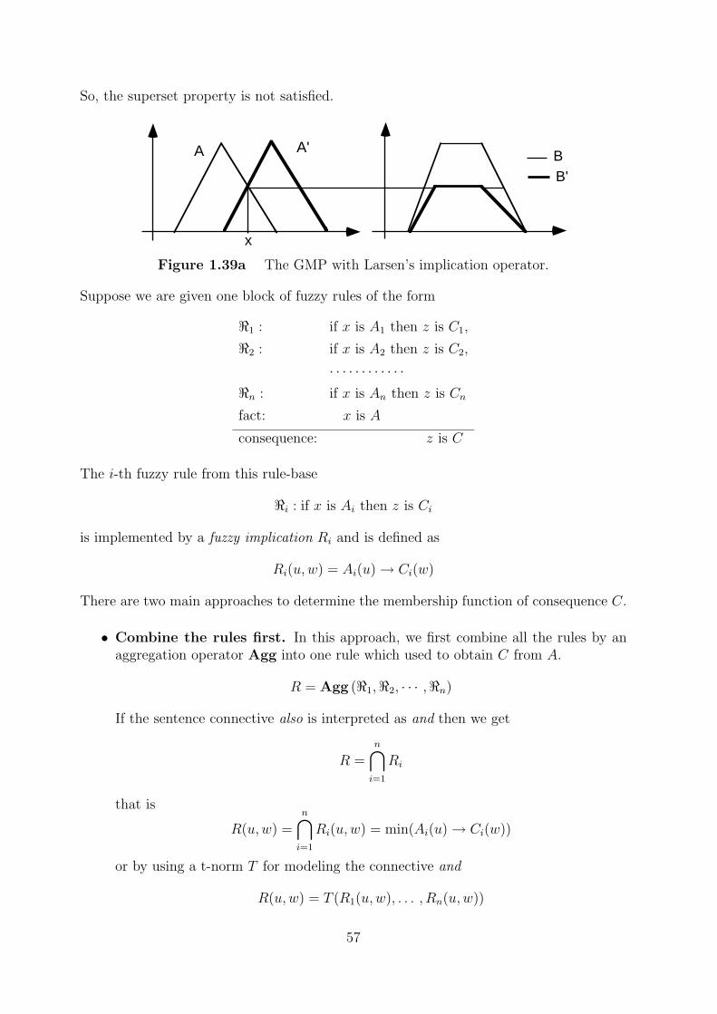
A B
x
B'
A'
So, the superset property is not satisfied.
Figure 1.39a The GMP with Larsen’s implication operator.
Suppose we are given one block of fuzzy rules of the form
<1 : if x is A1 then z is C1,
<2 : if x is A2 then z is C2,
· · · · · · · · · · · ·<n : if x is An then z is Cn
fact: x is A
consequence: z is C
The i-th fuzzy rule from this rule-base
<i : if x is Ai then z is Ci
is implemented by a fuzzy implication Ri and is defined as
Ri(u,w) = Ai(u)→ Ci(w)
There are two main approaches to determine the membership function of consequence C.
• Combine the rules first. In this approach, we first combine all the rules by anaggregation operator Agg into one rule which used to obtain C from A.
R = Agg (<1,<2, · · · ,<n)
If the sentence connective also is interpreted as and then we get
R =n⋂i=1
Ri
that is
R(u,w) =n⋂i=1
Ri(u,w) = min(Ai(u)→ Ci(w))
or by using a t-norm T for modeling the connective and
R(u,w) = T (R1(u,w), . . . , Rn(u,w))
57
If the sentence connective also is interpreted as or then we get
R =n⋃i=1
Ri
that is
R(u,w) =n⋃i=1
Ri(u, v, w) = max(Ai(u)→ Ci(w))
or by using a t-conorm S for modeling the connective or
R(u,w) = S(R1(u,w), . . . , Rn(u,w))
Then we compute C from A by the compositional rule of inference as
C = A ◦R = A ◦Agg (R1, R2, · · · , Rn)
• Fire the rules first. Fire the rules individually, given A, and then combine theirresults into C.
We first compose A with each Ri producing intermediate result
C ′i = A ◦Ri
for i = 1, . . . , n and then combine the C ′i component wise into C ′ by some aggrega-tion operator Agg
C ′ = Agg (C ′1, . . . , C′n) = Agg (A ◦R1, . . . , A ◦Rn).
We show that the sup-min compositional operator and the connective also interpretedas the union operator are commutative. Thus the consequence, C, inferred from thecomplete set of rules is equivalent to the aggregated result, C ′, derived from individualrules.
Lemma 1.4.1 Let
C = A ◦n⋃i=1
Ri
be defined by standard sup-min composition as
C(w) = supu
min{A(u),max{R1(u,w), . . . , Rn(u,w)}}
and let
C ′ =n⋃i=1
A ◦Ri
defined by the sup-min composition as
C ′(w) = max{supuA(u) ∧Ri(u,w), . . . , sup
uA(u) ∧Rn(u,w)}.
Then C(w) = C ′(w) for all w from the universe of discourse W .
58
Proof. Using the distributivity of ∧ over ∨ we get
C(w) = supu{A(u) ∧ (R1(u,w) ∨ . . . ∨Rn(u,w))} = sup
u{(A(u) ∧R1(u,w)) ∨ . . .∨
(A(u) ∧Rn(u,w))} = max{supuA(u) ∧R1(u,w), . . . , sup
uA(u) ∧Rn(u,w)} = C ′(w).
Which ends the proof.
Similar statement holds for the sup-product compositional rule of inference, i.e the sup-product compositional operator and the connective also as the union operator are com-mutative.
Lemma 1.4.2 Let
C = A ◦n⋃i=1
Ri
be defined by sup-product composition as
C(w) = supuA(u) max{R1(u,w), . . . , Rn(u,w)}
and let
C ′ =n⋃i=1
A ◦Ri
defined by the sup-product composition as
C ′(w) = max{supuA(u)Ri(u,w), . . . , sup
uA(u)Rn(u,w)}
Then C(w) = C ′(w) holds for each w from the universe of discourse W .
Proof. Using the distributivity of multiplication over ∨ we have
C(w) = supu{A(u)(R1(u,w) ∨ . . . ∨Rn(u,w))} = sup
u{A(u)R1(u,w) ∨ . . .∨
A(u)Rn(u,w)} = max{supuA(u)R1(u,w), . . . , sup
uA(u)Rn(u,w)} = C ′(w).
Which ends the proof.
However, the sup-min compositional operator and the connective also interpreted as theintersection operator are not usually commutative. In this case, the consequence, C,inferred from the complete set of rules is included in the aggregated result, C ′, derivedfrom individual rules.
Lemma 1.4.3 Let
C = A ◦n⋂i=1
Ri
be defined by standard sup-min composition as
C(w) = supu
min{A(u),min{R1(u,w), . . . , Rn(u,w)}}
59
and let
C ′ =n⋂i=1
A ◦Ri
defined by the sup-min composition as
C ′(w) = min{supu{A(u) ∧Ri(u,w)}, . . . , sup
u{A(u) ∧Rn(u,w)}}.
Then C ⊂ C ′, i.e C(w) ≤ C ′(w) holds for all w from the universe of discourse W .
Proof. From the relationship
A ◦n⋂i=1
Ri ⊂ A ◦Ri
for each i = 1, . . . , n, we get
A ◦n⋂i=1
Ri ⊂n⋂i=1
A ◦Ri.
Which ends the proof.
Similar statement holds for the sup-t-norm compositional rule of inference, i.e the sup-product compositional operator and the connective also interpreted as the intersectionoperator are not commutative. In this case, the consequence, C, inferred from the com-plete set of rules is included in the aggregated result, C ′, derived from individual rules.
Lemma 1.4.4 Let
C = A ◦n⋂i=1
Ri
be defined by sup-T composition as
C(w) = supuT (A(u),min{R1(u,w), . . . , Rn(u,w)})
and let
C ′ =n⋂i=1
A ◦Ri
defined by the sup-T composition as
C ′(w) = min{supuT (A(u), Ri(u,w)), . . . , sup
uT (A(u), Rn(u,w))}.
Then C ⊂ C ′, i.e C(w) ≤ C ′(w) holds for all w from the universe of discourse W .
Example 1.4.3 We illustrate Lemma 1.4.3 by a simple example. Assume we have twofuzzy rules of the form
<1 : if x is A1 then z is C1
<2 : if x is A2 then z is C2
where A1, A2 and C1, C2 are discrete fuzzy numbers of the universe of discourses {x1, x2}and {z1, z2}, respectively. Suppose that we input a fuzzy set A = a1/x1 + a2/x2 to thesystem and let
60
R1 =
z1 z2
x1 0 1
x2 1 0
, R2 =
z1 z2
x1 1 0
x2 0 1
represent the fuzzy rules. We first compute the consequence C by
C = A ◦ (R1 ∩R2).
Using the definition of intersection of fuzzy relations we get
C = (a1/x1 + a2/x2) ◦
z1 z2
x1 0 1
x2 1 0
⋂ z1 z2
x1 1 0
x2 0 1
=
(a1/x1 + a2/x2) ◦
z1 z2
x1 0 0
x2 0 0
= ∅
Let us compute now the membership function of the consequence C ′ by
C ′ = (A ◦R1) ∩ (A ◦R2)
Using the definition of sup-min composition we get
A ◦R1 = (a1/x1 + a2/x2) ◦
z1 z2
x1 0 1
x2 1 0
.
Plugging into numerical values
(A ◦R1)(z1) = max{a1 ∧ 0, a2 ∧ 1} = a2, (A ◦R1)(z2) = max{a1 ∧ 1, a2 ∧ 0} = a1,
So,A ◦R1 = a2/z1 + a1/z2
and from
A ◦R2 = (a1/x1 + a2/x2) ◦
z1 z2
x1 1 0
x2 0 1
=
we getA ◦R2 = a1/z1 + a2/z2.
Finally,C ′ = a2/z1 + a1/z2 ∩ a1/z1 + a2/z2 = a1 ∧ a2/z1 + a1 ∧ a2/z2.
Which means that C is a proper subset of C ′ whenever min{a1, a2} 6= 0.
Suppose now that the fact of the GMP is given by a fuzzy singleton. Then the process ofcomputation of the membership function of the consequence becomes very simple.
61
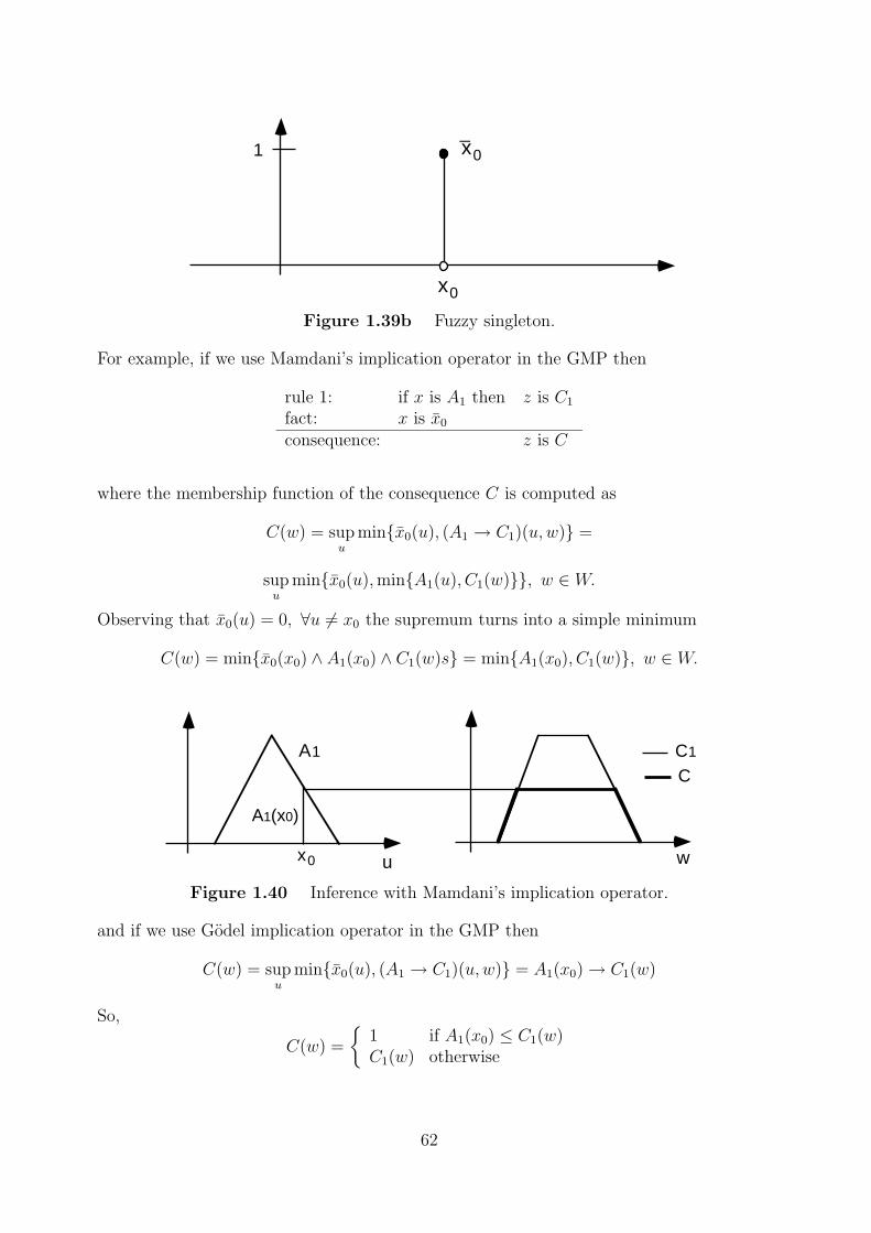
1
x0
x0_
A1 C1
x0 wu
A1(x0)
C
Figure 1.39b Fuzzy singleton.
For example, if we use Mamdani’s implication operator in the GMP then
rule 1: if x is A1 then z is C1
fact: x is x0
consequence: z is C
where the membership function of the consequence C is computed as
C(w) = supu
min{x0(u), (A1 → C1)(u,w)} =
supu
min{x0(u),min{A1(u), C1(w)}}, w ∈ W.
Observing that x0(u) = 0, ∀u 6= x0 the supremum turns into a simple minimum
C(w) = min{x0(x0) ∧ A1(x0) ∧ C1(w)s} = min{A1(x0), C1(w)}, w ∈W.
Figure 1.40 Inference with Mamdani’s implication operator.
and if we use Godel implication operator in the GMP then
C(w) = supu
min{x0(u), (A1 → C1)(u,w)} = A1(x0)→ C1(w)
So,
C(w) =
{1 if A1(x0) ≤ C1(w)C1(w) otherwise
62
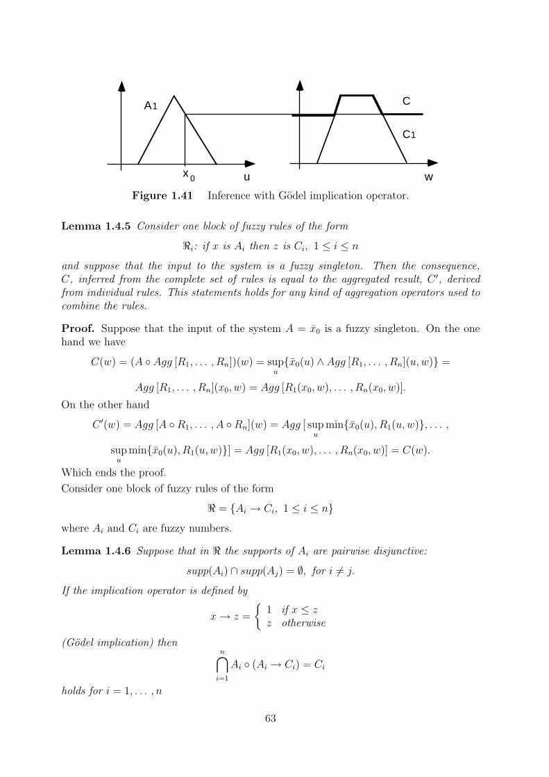
A1
u w
C1
C
x 0
Figure 1.41 Inference with Godel implication operator.
Lemma 1.4.5 Consider one block of fuzzy rules of the form
<i: if x is Ai then z is Ci, 1 ≤ i ≤ n
and suppose that the input to the system is a fuzzy singleton. Then the consequence,C, inferred from the complete set of rules is equal to the aggregated result, C ′, derivedfrom individual rules. This statements holds for any kind of aggregation operators used tocombine the rules.
Proof. Suppose that the input of the system A = x0 is a fuzzy singleton. On the onehand we have
C(w) = (A ◦ Agg [R1, . . . , Rn])(w) = supu{x0(u) ∧ Agg [R1, . . . , Rn](u,w)} =
Agg [R1, . . . , Rn](x0, w) = Agg [R1(x0, w), . . . , Rn(x0, w)].
On the other hand
C ′(w) = Agg [A ◦R1, . . . , A ◦Rn](w) = Agg [ supu
min{x0(u), R1(u,w)}, . . . ,
supu
min{x0(u), R1(u,w)}] = Agg [R1(x0, w), . . . , Rn(x0, w)] = C(w).
Which ends the proof.
Consider one block of fuzzy rules of the form
< = {Ai → Ci, 1 ≤ i ≤ n}where Ai and Ci are fuzzy numbers.
Lemma 1.4.6 Suppose that in < the supports of Ai are pairwise disjunctive:
supp(Ai) ∩ supp(Aj) = ∅, for i 6= j.
If the implication operator is defined by
x→ z =
{1 if x ≤ zz otherwise
(Godel implication) thenn⋂i=1
Ai ◦ (Ai → Ci) = Ci
holds for i = 1, . . . , n
63
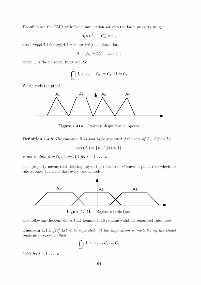
A1 A2 A3 A4
A1 A2 A3
Proof. Since the GMP with Godel implication satisfies the basic property we get
Ai ◦ (Ai → Ci) = Ai.
From supp(Ai) ∩ supp(Aj) = ∅, for i 6= j it follows that
Ai ◦ (Aj → Cj) = 1, i 6= j
where 1 is the universal fuzzy set. So,
n⋂i=1
Ai ◦ (Ai → Ci) = Ci ∩ 1 = Ci
Which ends the proof.
Figure 1.41a Pairwise disjunctive supports.
Definition 1.4.8 The rule-base < is said to be separated if the core of Ai, defined by
core(Ai) = {x | Ai(x) = 1},
is not contained in ∩j 6=isupp(Aj) for i = 1, . . . , n.
This property means that deleting any of the rules from < leaves a point x to which norule applies. It means that every rule is useful.
Figure 1.41b Separated rule-base.
The following theorem shows that Lemma 1.4.6 remains valid for separated rule-bases.
Theorem 1.4.1 [23] Let < be separated. If the implication is modelled by the Godelimplication operator then
n⋂i=1
Ai ◦ (Ai → Ci) = Ci
holds for i = 1, . . . , n
64
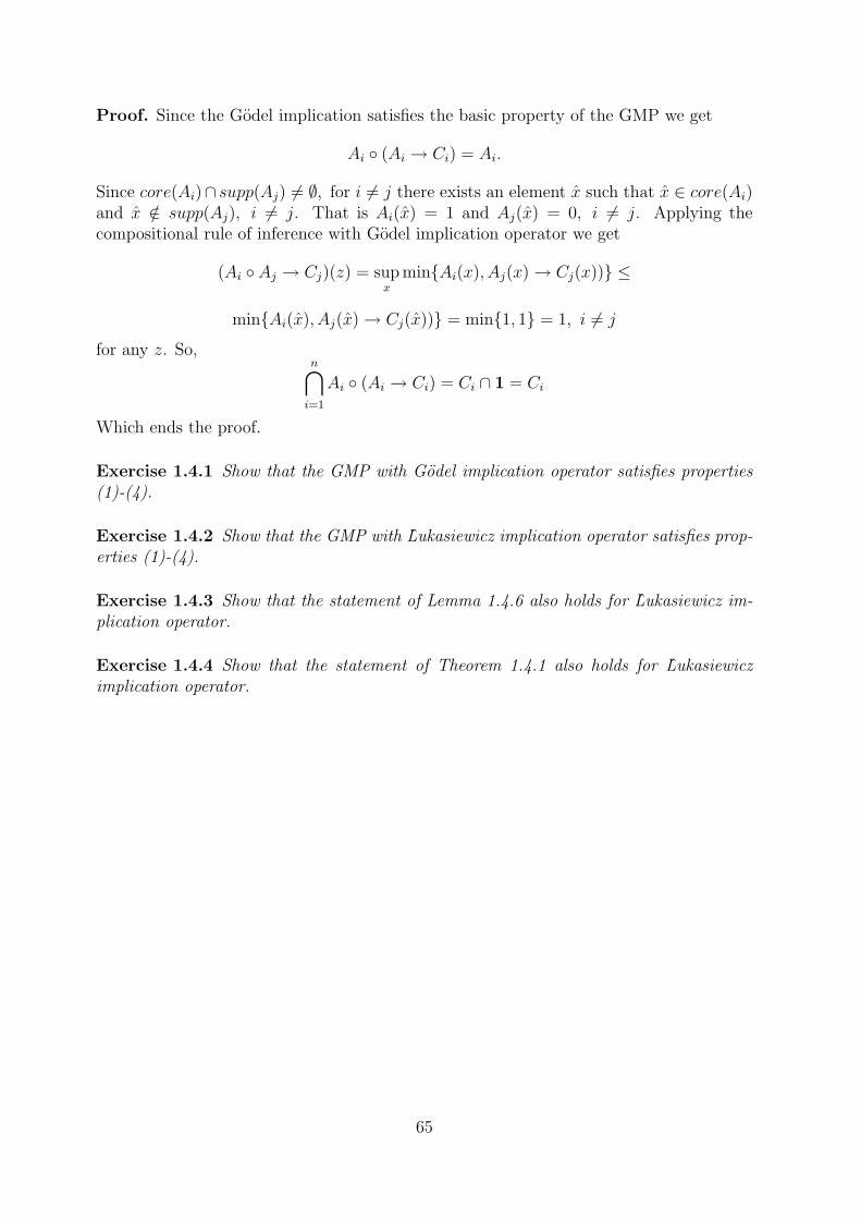
Proof. Since the Godel implication satisfies the basic property of the GMP we get
Ai ◦ (Ai → Ci) = Ai.
Since core(Ai)∩ supp(Aj) 6= ∅, for i 6= j there exists an element x such that x ∈ core(Ai)and x /∈ supp(Aj), i 6= j. That is Ai(x) = 1 and Aj(x) = 0, i 6= j. Applying thecompositional rule of inference with Godel implication operator we get
(Ai ◦ Aj → Cj)(z) = supx
min{Ai(x), Aj(x)→ Cj(x))} ≤
min{Ai(x), Aj(x)→ Cj(x))} = min{1, 1} = 1, i 6= j
for any z. So,n⋂i=1
Ai ◦ (Ai → Ci) = Ci ∩ 1 = Ci
Which ends the proof.
Exercise 1.4.1 Show that the GMP with Godel implication operator satisfies properties(1)-(4).
Exercise 1.4.2 Show that the GMP with ÃLukasiewicz implication operator satisfies prop-erties (1)-(4).
Exercise 1.4.3 Show that the statement of Lemma 1.4.6 also holds for ÃLukasiewicz im-plication operator.
Exercise 1.4.4 Show that the statement of Theorem 1.4.1 also holds for ÃLukasiewiczimplication operator.
65
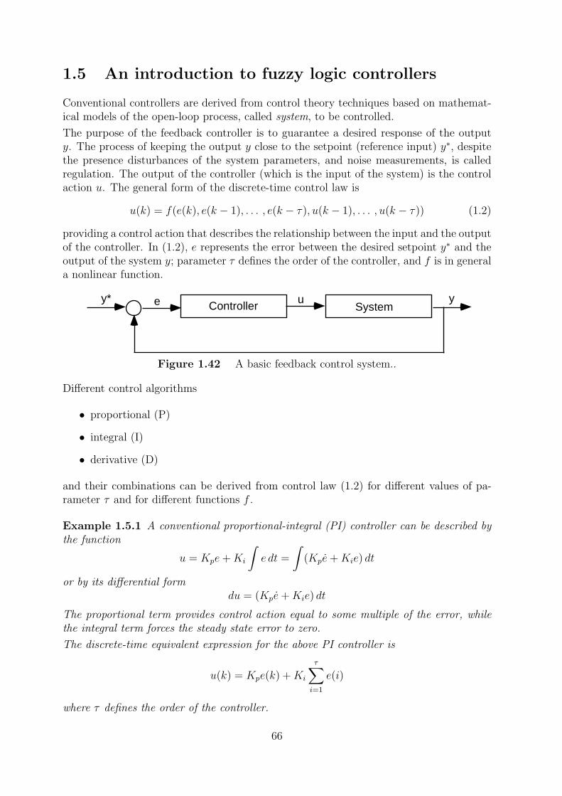
Controller Systemy* e u y
1.5 An introduction to fuzzy logic controllers
Conventional controllers are derived from control theory techniques based on mathemat-ical models of the open-loop process, called system, to be controlled.
The purpose of the feedback controller is to guarantee a desired response of the outputy. The process of keeping the output y close to the setpoint (reference input) y∗, despitethe presence disturbances of the system parameters, and noise measurements, is calledregulation. The output of the controller (which is the input of the system) is the controlaction u. The general form of the discrete-time control law is
u(k) = f(e(k), e(k − 1), . . . , e(k − τ), u(k − 1), . . . , u(k − τ)) (1.2)
providing a control action that describes the relationship between the input and the outputof the controller. In (1.2), e represents the error between the desired setpoint y∗ and theoutput of the system y; parameter τ defines the order of the controller, and f is in generala nonlinear function.
Figure 1.42 A basic feedback control system..
Different control algorithms
• proportional (P)
• integral (I)
• derivative (D)
and their combinations can be derived from control law (1.2) for different values of pa-rameter τ and for different functions f .
Example 1.5.1 A conventional proportional-integral (PI) controller can be described bythe function
u = Kpe+Ki
∫e dt =
∫(Kpe+Kie) dt
or by its differential formdu = (Kpe+Kie) dt
The proportional term provides control action equal to some multiple of the error, whilethe integral term forces the steady state error to zero.
The discrete-time equivalent expression for the above PI controller is
u(k) = Kpe(k) +Ki
τ∑i=1
e(i)
where τ defines the order of the controller.
66
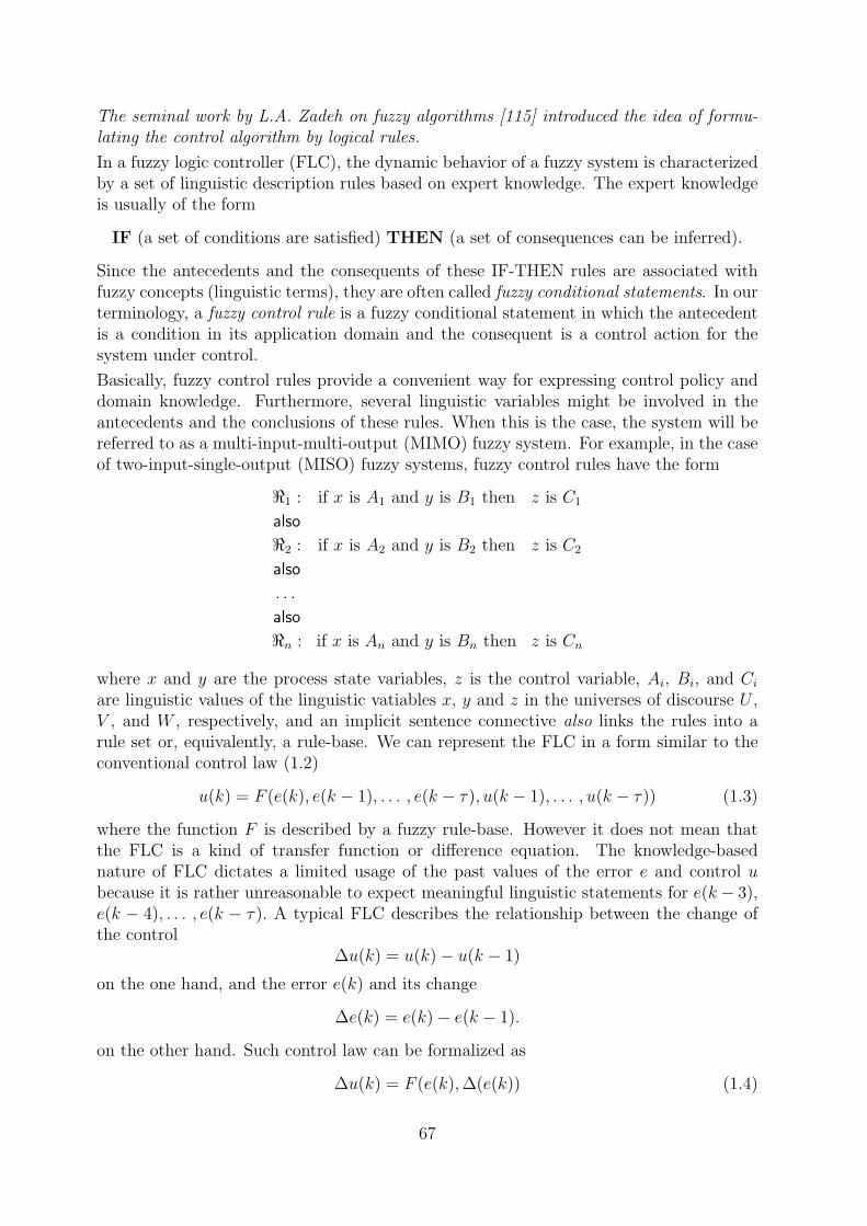
The seminal work by L.A. Zadeh on fuzzy algorithms [115] introduced the idea of formu-lating the control algorithm by logical rules.
In a fuzzy logic controller (FLC), the dynamic behavior of a fuzzy system is characterizedby a set of linguistic description rules based on expert knowledge. The expert knowledgeis usually of the form
IF (a set of conditions are satisfied) THEN (a set of consequences can be inferred).
Since the antecedents and the consequents of these IF-THEN rules are associated withfuzzy concepts (linguistic terms), they are often called fuzzy conditional statements. In ourterminology, a fuzzy control rule is a fuzzy conditional statement in which the antecedentis a condition in its application domain and the consequent is a control action for thesystem under control.
Basically, fuzzy control rules provide a convenient way for expressing control policy anddomain knowledge. Furthermore, several linguistic variables might be involved in theantecedents and the conclusions of these rules. When this is the case, the system will bereferred to as a multi-input-multi-output (MIMO) fuzzy system. For example, in the caseof two-input-single-output (MISO) fuzzy systems, fuzzy control rules have the form
<1 : if x is A1 and y is B1 then z is C1
also
<2 : if x is A2 and y is B2 then z is C2
also
. . .
also
<n : if x is An and y is Bn then z is Cn
where x and y are the process state variables, z is the control variable, Ai, Bi, and Ciare linguistic values of the linguistic vatiables x, y and z in the universes of discourse U ,V , and W , respectively, and an implicit sentence connective also links the rules into arule set or, equivalently, a rule-base. We can represent the FLC in a form similar to theconventional control law (1.2)
u(k) = F (e(k), e(k − 1), . . . , e(k − τ), u(k − 1), . . . , u(k − τ)) (1.3)
where the function F is described by a fuzzy rule-base. However it does not mean thatthe FLC is a kind of transfer function or difference equation. The knowledge-basednature of FLC dictates a limited usage of the past values of the error e and control ubecause it is rather unreasonable to expect meaningful linguistic statements for e(k − 3),e(k − 4), . . . , e(k − τ). A typical FLC describes the relationship between the change ofthe control
∆u(k) = u(k)− u(k − 1)
on the one hand, and the error e(k) and its change
∆e(k) = e(k)− e(k − 1).
on the other hand. Such control law can be formalized as
∆u(k) = F (e(k),∆(e(k)) (1.4)
67
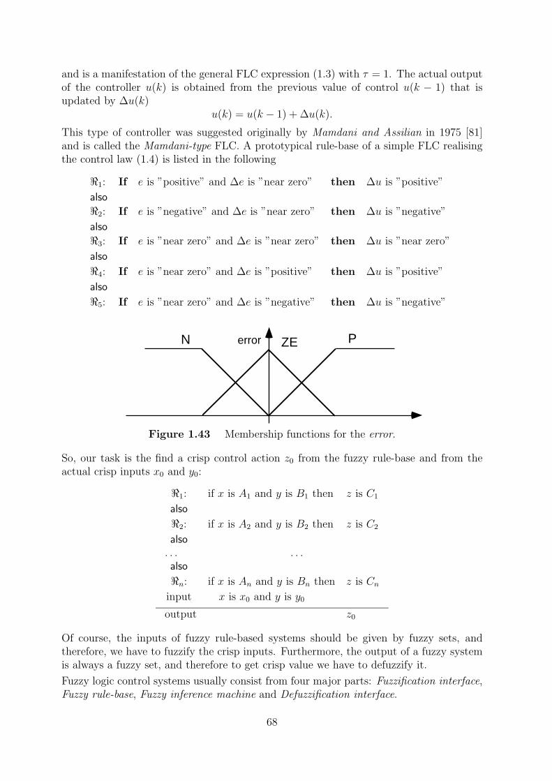
N PZEerror
and is a manifestation of the general FLC expression (1.3) with τ = 1. The actual outputof the controller u(k) is obtained from the previous value of control u(k − 1) that isupdated by ∆u(k)
u(k) = u(k − 1) + ∆u(k).
This type of controller was suggested originally by Mamdani and Assilian in 1975 [81]and is called the Mamdani-type FLC. A prototypical rule-base of a simple FLC realisingthe control law (1.4) is listed in the following
<1: If e is ”positive” and ∆e is ”near zero” then ∆u is ”positive”
also
<2: If e is ”negative” and ∆e is ”near zero” then ∆u is ”negative”
also
<3: If e is ”near zero” and ∆e is ”near zero” then ∆u is ”near zero”
also
<4: If e is ”near zero” and ∆e is ”positive” then ∆u is ”positive”
also
<5: If e is ”near zero” and ∆e is ”negative” then ∆u is ”negative”
Figure 1.43 Membership functions for the error.
So, our task is the find a crisp control action z0 from the fuzzy rule-base and from theactual crisp inputs x0 and y0:
<1: if x is A1 and y is B1 then z is C1
also
<2: if x is A2 and y is B2 then z is C2
also. . . . . .
also
<n: if x is An and y is Bn then z is Cninput x is x0 and y is y0
output z0
Of course, the inputs of fuzzy rule-based systems should be given by fuzzy sets, andtherefore, we have to fuzzify the crisp inputs. Furthermore, the output of a fuzzy systemis always a fuzzy set, and therefore to get crisp value we have to defuzzify it.
Fuzzy logic control systems usually consist from four major parts: Fuzzification interface,Fuzzy rule-base, Fuzzy inference machine and Defuzzification interface.
68
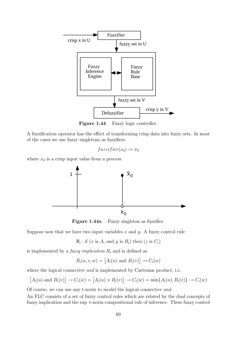
Defuzzifier
fuzzy set in U
fuzzy set in V
Fuzzifier
FuzzyInference Engine
crisp x in U
crisp y in V
FuzzyRule Base
1
x0
x0_
Figure 1.44 Fuzzy logic controller.
A fuzzification operator has the effect of transforming crisp data into fuzzy sets. In mostof the cases we use fuzzy singletons as fuzzifiers
fuzzifier(x0) := x0
where x0 is a crisp input value from a process.
Figure 1.44a Fuzzy singleton as fuzzifier.
Suppose now that we have two input variables x and y. A fuzzy control rule
<i : if (x is Ai and y is Bi) then (z is Ci)
is implemented by a fuzzy implication Ri and is defined as
Ri(u, v, w) =[Ai(u) and Bi(v)
]→ Ci(w)
where the logical connective and is implemented by Cartesian product, i.e.[Ai(u) and Bi(v)
]→ Ci(w) =
[Ai(u)×Bi(v)
]→ Ci(w) = min{Ai(u), Bi(v)} → Ci(w)
Of course, we can use any t-norm to model the logical connective and.
An FLC consists of a set of fuzzy control rules which are related by the dual concepts offuzzy implication and the sup–t-norm compositional rule of inference. These fuzzy control
69
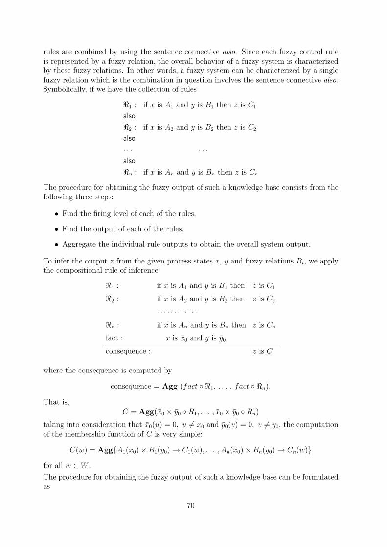
rules are combined by using the sentence connective also. Since each fuzzy control ruleis represented by a fuzzy relation, the overall behavior of a fuzzy system is characterizedby these fuzzy relations. In other words, a fuzzy system can be characterized by a singlefuzzy relation which is the combination in question involves the sentence connective also.Symbolically, if we have the collection of rules
<1 : if x is A1 and y is B1 then z is C1
also
<2 : if x is A2 and y is B2 then z is C2
also
· · · · · ·also
<n : if x is An and y is Bn then z is Cn
The procedure for obtaining the fuzzy output of such a knowledge base consists from thefollowing three steps:
• Find the firing level of each of the rules.
• Find the output of each of the rules.
• Aggregate the individual rule outputs to obtain the overall system output.
To infer the output z from the given process states x, y and fuzzy relations Ri, we applythe compositional rule of inference:
<1 : if x is A1 and y is B1 then z is C1
<2 : if x is A2 and y is B2 then z is C2
· · · · · · · · · · · ·<n : if x is An and y is Bn then z is Cn
fact : x is x0 and y is y0
consequence : z is C
where the consequence is computed by
consequence = Agg (fact ◦ <1, . . . , fact ◦ <n).
That is,C = Agg(x0 × y0 ◦R1, . . . , x0 × y0 ◦Rn)
taking into consideration that x0(u) = 0, u 6= x0 and y0(v) = 0, v 6= y0, the computationof the membership function of C is very simple:
C(w) = Agg{A1(x0)×B1(y0)→ C1(w), . . . , An(x0)×Bn(y0)→ Cn(w)}
for all w ∈W .
The procedure for obtaining the fuzzy output of such a knowledge base can be formulatedas
70
• The firing level of the i-th rule is determined by
Ai(x0)×Bi(y0).
• The output of of the i-th rule is calculated by
C ′i(w) := Ai(x0)×Bi(y0)→ Ci(w)
for all w ∈W .
• The overall system output, C, is obtained from the individual rule outputs C ′i by
C(w) = Agg{C ′1, . . . , C ′n}
for all w ∈W .
Example 1.5.2 If the sentence connective also is interpreted as anding the rules by usingminimum-norm then the membership function of the consequence is computed as
C = (x0 × y0 ◦R1) ∩ . . . ∩ (x0 × y0 ◦Rn).
That is,
C(w) = min{A1(x0)×B1(y0)→ C1(w), . . . , An(x0)×Bn(y0)→ Cn(w)}
for all w ∈W .
Example 1.5.3 If the sentence connective also is interpreted as oring the rules by usingminimum-norm then the membership function of the consequence is computed as
C = (x0 × y0 ◦R1) ∪ . . . ∪ (x0 × y0 ◦Rn).
That is,
C(w) = max{A1(x0)×B1(y0)→ C1(w), . . . , An(x0)×Bn(y0)→ Cn(w)}
for all w ∈W .
Example 1.5.4 Suppose that the Cartesian product and the implication operator are im-plemented by the t-norm T (u, v) = uv. If the sentence connective also is interpreted asoring the rules by using minimum-norm then the membership function of the consequenceis computed as
C = (x0 × y0 ◦R1) ∪ . . . ∪ (x0 × y0 ◦Rn).
That is,C(w) = max{A1(x0)B1(y0)C1(w), . . . , An(x0)Bn(y0)Cn(w)}
for all w ∈W .
71
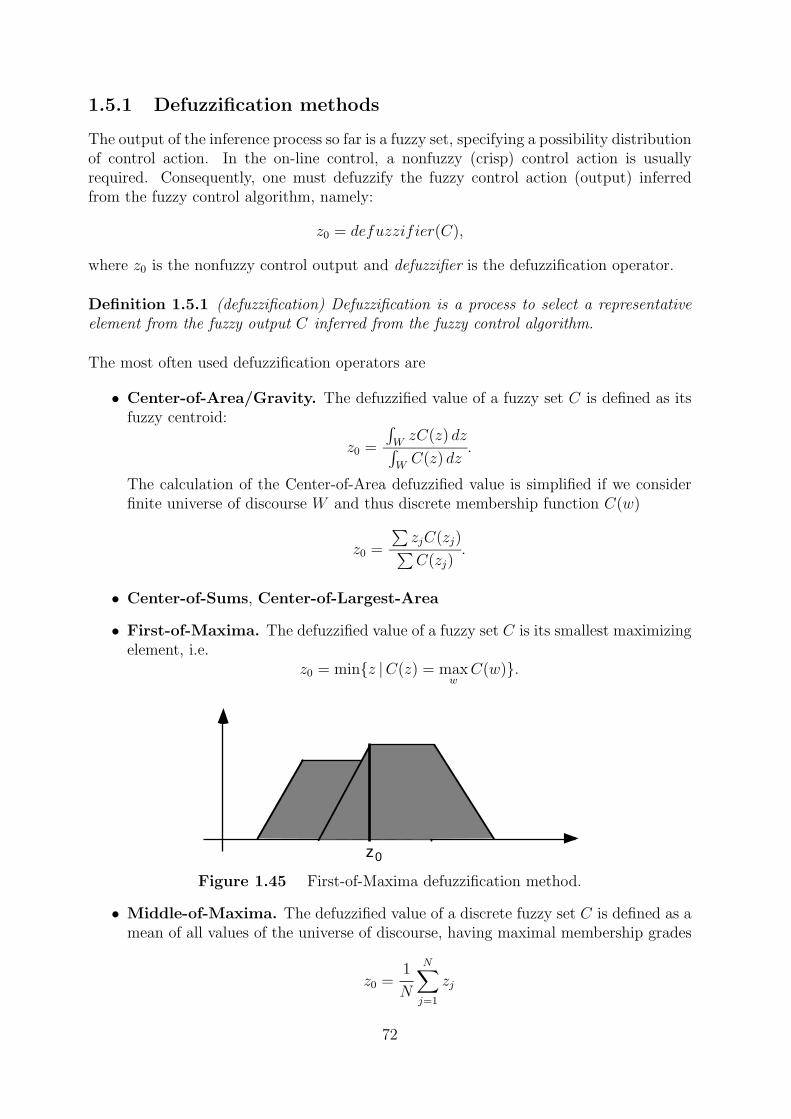
z0
1.5.1 Defuzzification methods
The output of the inference process so far is a fuzzy set, specifying a possibility distributionof control action. In the on-line control, a nonfuzzy (crisp) control action is usuallyrequired. Consequently, one must defuzzify the fuzzy control action (output) inferredfrom the fuzzy control algorithm, namely:
z0 = defuzzifier(C),
where z0 is the nonfuzzy control output and defuzzifier is the defuzzification operator.
Definition 1.5.1 (defuzzification) Defuzzification is a process to select a representativeelement from the fuzzy output C inferred from the fuzzy control algorithm.
The most often used defuzzification operators are
• Center-of-Area/Gravity. The defuzzified value of a fuzzy set C is defined as itsfuzzy centroid:
z0 =
∫WzC(z) dz∫
WC(z) dz
.
The calculation of the Center-of-Area defuzzified value is simplified if we considerfinite universe of discourse W and thus discrete membership function C(w)
z0 =
∑zjC(zj)∑C(zj)
.
• Center-of-Sums, Center-of-Largest-Area
• First-of-Maxima. The defuzzified value of a fuzzy set C is its smallest maximizingelement, i.e.
z0 = min{z |C(z) = maxw
C(w)}.
Figure 1.45 First-of-Maxima defuzzification method.
• Middle-of-Maxima. The defuzzified value of a discrete fuzzy set C is defined as amean of all values of the universe of discourse, having maximal membership grades
z0 =1
N
N∑j=1
zj
72
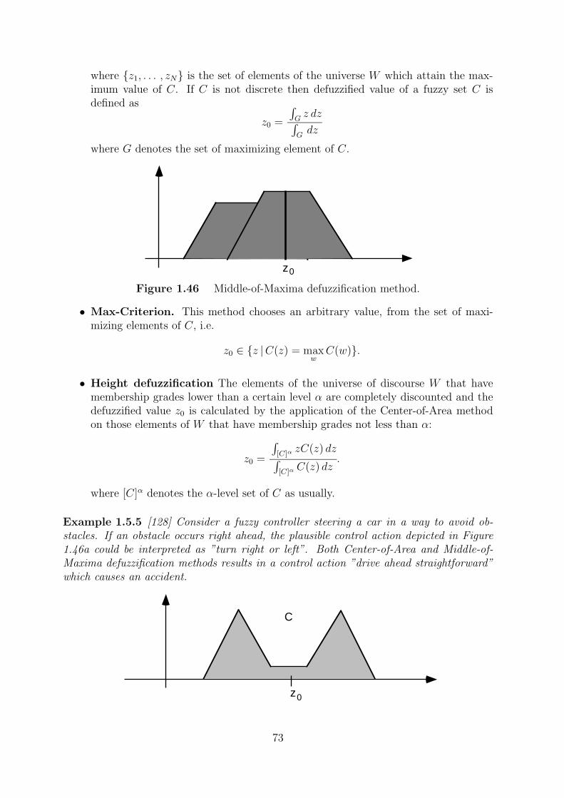
z0
C
z0
where {z1, . . . , zN} is the set of elements of the universe W which attain the max-imum value of C. If C is not discrete then defuzzified value of a fuzzy set C isdefined as
z0 =
∫Gz dz∫
Gdz
where G denotes the set of maximizing element of C.
Figure 1.46 Middle-of-Maxima defuzzification method.
• Max-Criterion. This method chooses an arbitrary value, from the set of maxi-mizing elements of C, i.e.
z0 ∈ {z |C(z) = maxw
C(w)}.
• Height defuzzification The elements of the universe of discourse W that havemembership grades lower than a certain level α are completely discounted and thedefuzzified value z0 is calculated by the application of the Center-of-Area methodon those elements of W that have membership grades not less than α:
z0 =
∫[C]α
zC(z) dz∫[C]α
C(z) dz.
where [C]α denotes the α-level set of C as usually.
Example 1.5.5 [128] Consider a fuzzy controller steering a car in a way to avoid ob-stacles. If an obstacle occurs right ahead, the plausible control action depicted in Figure1.46a could be interpreted as ”turn right or left”. Both Center-of-Area and Middle-of-Maxima defuzzification methods results in a control action ”drive ahead straightforward”which causes an accident.
73
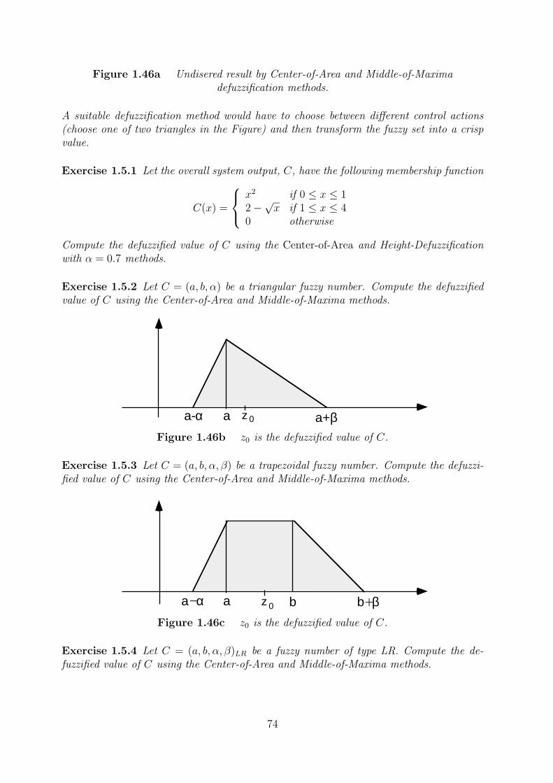
aa-α a+βz 0
aa- α b+βbz 0
Figure 1.46a Undisered result by Center-of-Area and Middle-of-Maximadefuzzification methods.
A suitable defuzzification method would have to choose between different control actions(choose one of two triangles in the Figure) and then transform the fuzzy set into a crispvalue.
Exercise 1.5.1 Let the overall system output, C, have the following membership function
C(x) =
x2 if 0 ≤ x ≤ 12−√x if 1 ≤ x ≤ 40 otherwise
Compute the defuzzified value of C using the Center-of-Area and Height-Defuzzificationwith α = 0.7 methods.
Exercise 1.5.2 Let C = (a, b, α) be a triangular fuzzy number. Compute the defuzzifiedvalue of C using the Center-of-Area and Middle-of-Maxima methods.
Figure 1.46b z0 is the defuzzified value of C.
Exercise 1.5.3 Let C = (a, b, α, β) be a trapezoidal fuzzy number. Compute the defuzzi-fied value of C using the Center-of-Area and Middle-of-Maxima methods.
Figure 1.46c z0 is the defuzzified value of C.
Exercise 1.5.4 Let C = (a, b, α, β)LR be a fuzzy number of type LR. Compute the de-fuzzified value of C using the Center-of-Area and Middle-of-Maxima methods.
74
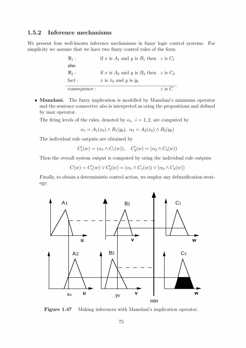
u v
C1
w
uxo v
C2
wyo
min
A1
A2
B1
B2
1.5.2 Inference mechanisms
We present four well-known inference mechanisms in fuzzy logic control systems. Forsimplicity we assume that we have two fuzzy control rules of the form
<1 : if x is A1 and y is B1 then z is C1
also
<2 : if x is A2 and y is B2 then z is C2
fact : x is x0 and y is y0
consequence : z is C
• Mamdani. The fuzzy implication is modelled by Mamdani’s minimum operatorand the sentence connective also is interpreted as oring the propositions and definedby max operator.
The firing levels of the rules, denoted by αi, i = 1, 2, are computed by
α1 = A1(x0) ∧B1(y0), α2 = A2(x0) ∧B2(y0)
The individual rule outputs are obtained by
C ′1(w) = (α1 ∧ C1(w)), C ′2(w) = (α2 ∧ C2(w))
Then the overall system output is computed by oring the individual rule outputs
C(w) = C ′1(w) ∨ C ′2(w) = (α1 ∧ C1(w)) ∨ (α2 ∧ C2(w))
Finally, to obtain a deterministic control action, we employ any defuzzification strat-egy.
Figure 1.47 Making inferences with Mamdani’s implication operator.
75
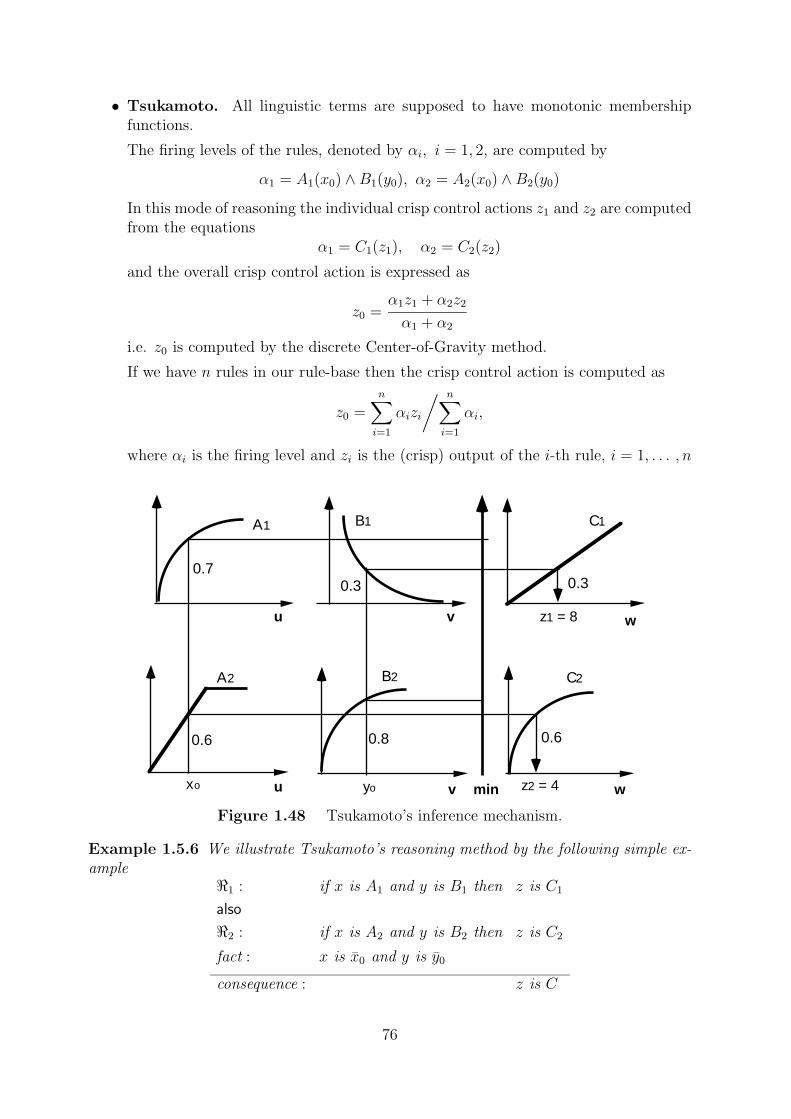
u v w
uxo vyo wmin
A1
B2
C1
A2
B1
C2
0.3
0.6 0.8 0.6
z2 = 4
z1 = 8
0.70.3
• Tsukamoto. All linguistic terms are supposed to have monotonic membershipfunctions.
The firing levels of the rules, denoted by αi, i = 1, 2, are computed by
α1 = A1(x0) ∧B1(y0), α2 = A2(x0) ∧B2(y0)
In this mode of reasoning the individual crisp control actions z1 and z2 are computedfrom the equations
α1 = C1(z1), α2 = C2(z2)
and the overall crisp control action is expressed as
z0 =α1z1 + α2z2
α1 + α2
i.e. z0 is computed by the discrete Center-of-Gravity method.
If we have n rules in our rule-base then the crisp control action is computed as
z0 =n∑i=1
αizi
/ n∑i=1
αi,
where αi is the firing level and zi is the (crisp) output of the i-th rule, i = 1, . . . , n
Figure 1.48 Tsukamoto’s inference mechanism.
Example 1.5.6 We illustrate Tsukamoto’s reasoning method by the following simple ex-ample
<1 : if x is A1 and y is B1 then z is C1
also
<2 : if x is A2 and y is B2 then z is C2
fact : x is x0 and y is y0
consequence : z is C
76
Then according to Fig.1.48 we see that
A1(x0) = 0.7, B1(y0) = 0.3
therefore, the firing level of the first rule is
α1 = min{A1(x0), B1(y0)} = min{0.7, 0.3} = 0.3
and fromA2(x0) = 0.6, B2(y0) = 0.8
it follows that the firing level of the second rule is
α2 = min{A2(x0), B2(y0)} = min{0.6, 0.8} = 0.6
the individual rule outputs z1 = 8 and z2 = 4 are derived from the equations
C1(z1) = 0.3, C2(z2) = 0.6
and the crisp control action is
z0 = (8× 0.3 + 4× 0.6)/(0.3 + 0.6) = 6.
• Sugeno. Sugeno and Takagi use the following architecture [93]
<1 : if x is A1 and y is B1 then z1 = a1x+ b1y
also
<2 : if x is A2 and y is B2 then z2 = a2x+ b2y
fact : x is x0 and y is y0
consequence : z0
The firing levels of the rules are computed by
α1 = A1(x0) ∧B1(y0), α2 = A2(x0) ∧B2(y0)
then the individual rule outputs are derived from the relationships
z∗1 = a1x0 + b1y0, z∗2 = a2x0 + b2y0
and the crisp control action is expressed as
z0 =α1z
∗1 + α2z
∗2
α1 + α2
If we have n rules in our rule-base then the crisp control action is computed as
z0 =n∑i=1
αiz∗i
/ n∑i=1
αi,
where αi denotes the firing level of the i-th rule, i = 1, . . . , n
77
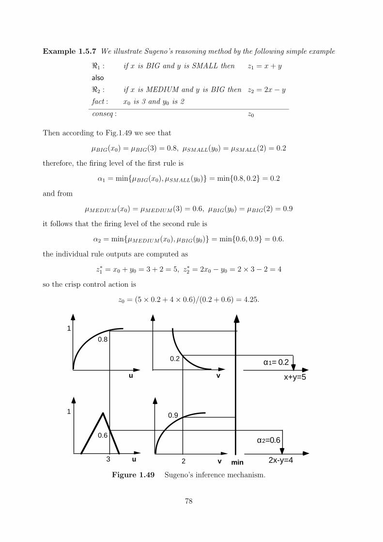
1
u v
1
u v2 min3
α1= 0.2
α2=0.6
x+y=5
2x-y=4
0.2
0.6
0.8
0.9
Example 1.5.7 We illustrate Sugeno’s reasoning method by the following simple example
<1 : if x is BIG and y is SMALL then z1 = x+ y
also
<2 : if x is MEDIUM and y is BIG then z2 = 2x− yfact : x0 is 3 and y0 is 2
conseq : z0
Then according to Fig.1.49 we see that
µBIG(x0) = µBIG(3) = 0.8, µSMALL(y0) = µSMALL(2) = 0.2
therefore, the firing level of the first rule is
α1 = min{µBIG(x0), µSMALL(y0)} = min{0.8, 0.2} = 0.2
and from
µMEDIUM(x0) = µMEDIUM(3) = 0.6, µBIG(y0) = µBIG(2) = 0.9
it follows that the firing level of the second rule is
α2 = min{µMEDIUM(x0), µBIG(y0)} = min{0.6, 0.9} = 0.6.
the individual rule outputs are computed as
z∗1 = x0 + y0 = 3 + 2 = 5, z∗2 = 2x0 − y0 = 2× 3− 2 = 4
so the crisp control action is
z0 = (5× 0.2 + 4× 0.6)/(0.2 + 0.6) = 4.25.
Figure 1.49 Sugeno’s inference mechanism.
78
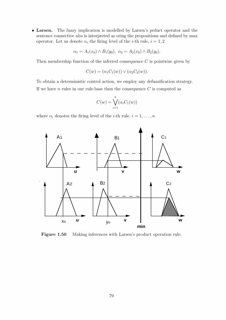
u v
C1
w
uxo v
C2
wyo
A1
A2
B1
B2
min
• Larsen. The fuzzy implication is modelled by Larsen’s prduct operator and thesentence connective also is interpreted as oring the propositions and defined by maxoperator. Let us denote αi the firing level of the i-th rule, i = 1, 2
α1 = A1(x0) ∧B1(y0), α2 = A2(x0) ∧B2(y0).
Then membership function of the inferred consequence C is pointwise given by
C(w) = (α1C1(w)) ∨ (α2C2(w)).
To obtain a deterministic control action, we employ any defuzzification strategy.
If we have n rules in our rule-base then the consequence C is computed as
C(w) =n∨i=1
(αiC1(w))
where αi denotes the firing level of the i-th rule, i = 1, . . . , n
Figure 1.50 Making inferences with Larsen’s product operation rule.
79
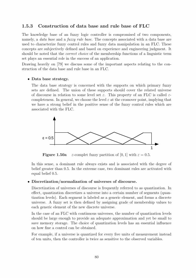
ε = 0.5
1
1.5.3 Construction of data base and rule base of FLC
The knowledge base of an fuzzy logic controller is compromised of two components,namely, a data base and a fuzzy rule base. The concepts associated with a data base areused to characterize fuzzy control rules and fuzzy data manipulation in an FLC. Theseconcepts are subjectively defined and based on experience and engineering judgment. Itshould be noted that the correct choice of the membership functions of a linguistic termset plays an essential role in the success of an application.
Drawing heavily on [79] we discuss some of the important aspects relating to the con-struction of the data base and rule base in an FLC.
• Data base strategy.
The data base strategy is concerned with the supports on which primary fuzzysets are defined. The union of these supports should cover the related universeof discourse in relation to some level set ε. This property of an FLC is called ε-completeness. In general, we choose the level ε at the crossover point, implying thatwe have a strong belief in the positive sense of the fuzzy control rules which areassociated with the FLC.
Figure 1.50a ε-complet fuzzy partition of [0, 1] with ε = 0.5.
In this sense, a dominant rule always exists and is associated with the degree ofbelief greater than 0.5. In the extreme case, two dominant rules are activated withequal belief 0.5.
• Discretization/normalization of universes of discourse.
Discretization of universes of discourse is frequently referred to as quantization. Ineffect, quantization discretizes a universe into a certain number of segments (quan-tization levels). Each segment is labeled as a generic element, and forms a discreteuniverse. A fuzzy set is then defined by assigning grade of membership values toeach generic element of the new discrete universe.
In the case of an FLC with continuous universes, the number of quantization levelsshould be large enough to provide an adequate approximation and yet be small tosave memory storage. The choice of quantization levels has an essential influenceon how fine a control can be obtained.
For example, if a universe is quantized for every five units of measurement insteadof ten units, then the controller is twice as sensitive to the observed variables.
80
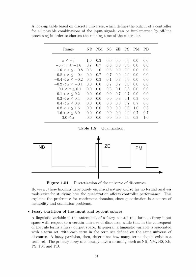
NB ZE PM
A look-up table based on discrete universes, which defines the output of a controllerfor all possible combinations of the input signals, can be implemented by off-lineprocessing in order to shorten the running time of the controller.
Range NB NM NS ZE PS PM PB
x ≤ −3 1.0 0.3 0.0 0.0 0.0 0.0 0.0−3 < x ≤ −1.6 0.7 0.7 0.0 0.0 0.0 0.0 0.0−1.6 < x ≤ −0.8 0.3 1.0 0.3 0.0 0.0 0.0 0.0−0.8 < x ≤ −0.4 0.0 0.7 0.7 0.0 0.0 0.0 0.0−0.4 < x ≤ −0.2 0.0 0.3 0.1 0.3 0.0 0.0 0.0−0.2 < x ≤ −0.1 0.0 0.0 0.7 0.7 0.0 0.0 0.0−0.1 < x ≤ 0.1 0.0 0.0 0.3 0.1 0.3 0.0 0.00.1 < x ≤ 0.2 0.0 0.0 0.0 0.7 0.7 0.0 0.00.2 < x ≤ 0.4 0.0 0.0 0.0 0.3 0.1 0.3 0.00.4 < x ≤ 0.8 0.0 0.0 0.0 0.0 0.7 0.7 0.00.8 < x ≤ 1.6 0.0 0.0 0.0 0.0 0.3 1.0 0.31.6 < x ≤ 3.0 0.0 0.0 0.0 0.0 0.0 0.7 0.7
3.0 ≤ x 0.0 0.0 0.0 0.0 0.0 0.3 1.0
Table 1.5 Quantization.
Figure 1.51 Discretization of the universe of discourses.
However, these findings have purely empirical nature and so far no formal analysistools exist for studying how the quantization affects controller performance. Thisexplains the preference for continuous domains, since quantization is a source ofinstability and oscillation problems.
• Fuzzy partition of the input and output spaces.
A linguistic variable in the antecedent of a fuzzy control rule forms a fuzzy inputspace with respect to a certain universe of discourse, while that in the consequentof the rule forms a fuzzy output space. In general, a linguistic variable is associatedwith a term set, with each term in the term set defined on the same universe ofdiscourse. A fuzzy partition, then, determines how many terms should exist in aterm set. The primary fuzzy sets usually have a meaning, such as NB, NM, NS, ZE,PS, PM and PB.
81
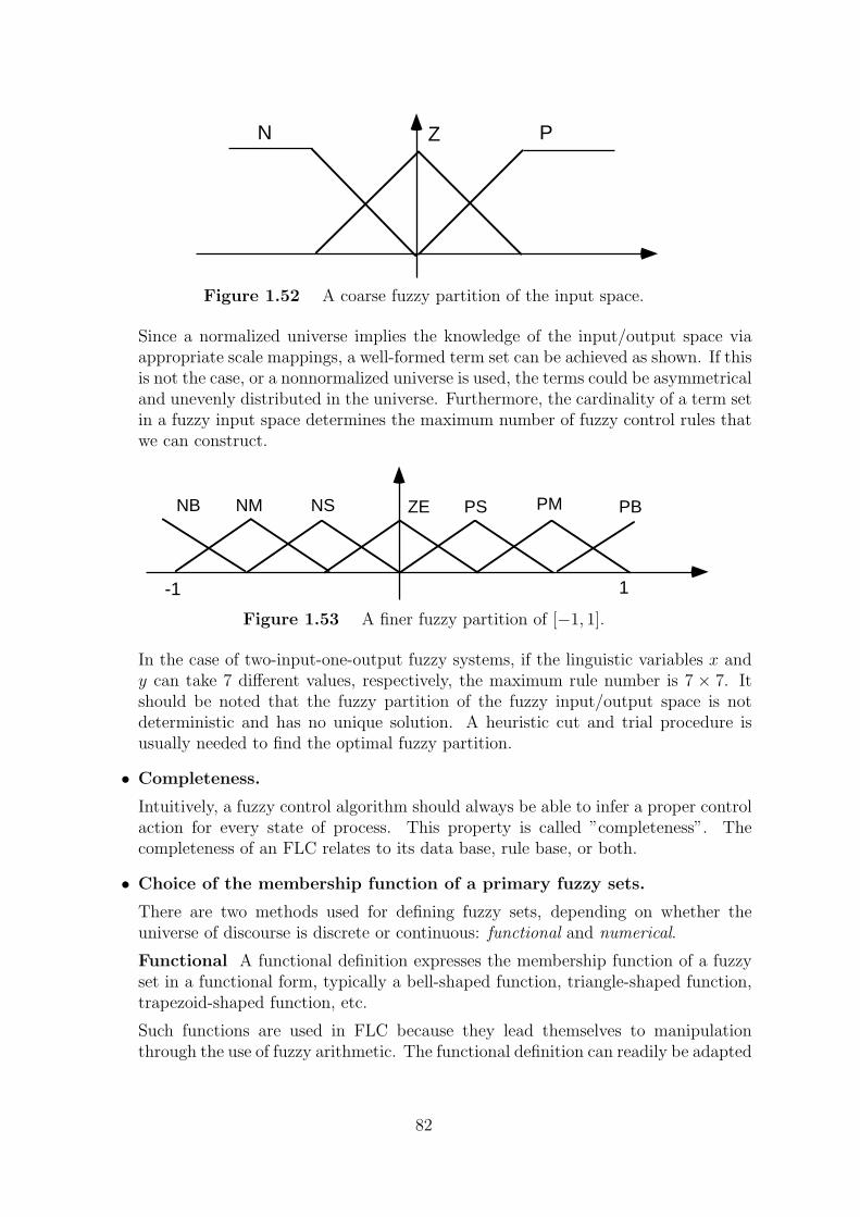
N Z P
NB PBPMPSZENSNM
-1 1
Figure 1.52 A coarse fuzzy partition of the input space.
Since a normalized universe implies the knowledge of the input/output space viaappropriate scale mappings, a well-formed term set can be achieved as shown. If thisis not the case, or a nonnormalized universe is used, the terms could be asymmetricaland unevenly distributed in the universe. Furthermore, the cardinality of a term setin a fuzzy input space determines the maximum number of fuzzy control rules thatwe can construct.
Figure 1.53 A finer fuzzy partition of [−1, 1].
In the case of two-input-one-output fuzzy systems, if the linguistic variables x andy can take 7 different values, respectively, the maximum rule number is 7 × 7. Itshould be noted that the fuzzy partition of the fuzzy input/output space is notdeterministic and has no unique solution. A heuristic cut and trial procedure isusually needed to find the optimal fuzzy partition.
• Completeness.
Intuitively, a fuzzy control algorithm should always be able to infer a proper controlaction for every state of process. This property is called ”completeness”. Thecompleteness of an FLC relates to its data base, rule base, or both.
• Choice of the membership function of a primary fuzzy sets.
There are two methods used for defining fuzzy sets, depending on whether theuniverse of discourse is discrete or continuous: functional and numerical.
Functional A functional definition expresses the membership function of a fuzzyset in a functional form, typically a bell-shaped function, triangle-shaped function,trapezoid-shaped function, etc.
Such functions are used in FLC because they lead themselves to manipulationthrough the use of fuzzy arithmetic. The functional definition can readily be adapted
82
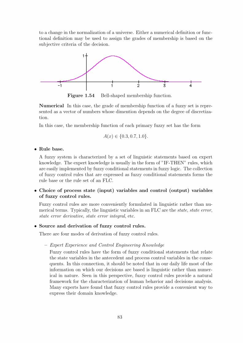
to a change in the normalization of a universe. Either a numerical definition or func-tional definition may be used to assign the grades of membership is based on thesubjective criteria of the decision.
Figure 1.54 Bell-shaped membership function.
Numerical In this case, the grade of membership function of a fuzzy set is repre-sented as a vector of numbers whose dimention depends on the degree of discretiza-tion.
In this case, the membership function of each primary fuzzy set has the form
A(x) ∈ {0.3, 0.7, 1.0}.
• Rule base.
A fuzzy system is characterized by a set of linguistic statements based on expertknowledge. The expert knowledge is usually in the form of ”IF-THEN” rules, whichare easily implemented by fuzzy conditional statements in fuzzy logic. The collectionof fuzzy control rules that are expressed as fuzzy conditional statements forms therule base or the rule set of an FLC.
• Choice of process state (input) variables and control (output) variablesof fuzzy control rules.
Fuzzy control rules are more conveniently formulated in linguistic rather than nu-merical terms. Typically, the linguistic variables in an FLC are the state, state error,state error derivative, state error integral, etc.
• Source and derivation of fuzzy control rules.
There are four modes of derivation of fuzzy control rules.
– Expert Experience and Control Engineering Knowledge
Fuzzy control rules have the form of fuzzy conditional statements that relatethe state variables in the antecedent and process control variables in the conse-quents. In this connection, it should be noted that in our daily life most of theinformation on which our decisions are based is linguistic rather than numer-ical in nature. Seen in this perspective, fuzzy control rules provide a naturalframework for the characterization of human behavior and decisions analysis.Many experts have found that fuzzy control rules provide a convenient way toexpress their domain knowledge.
83
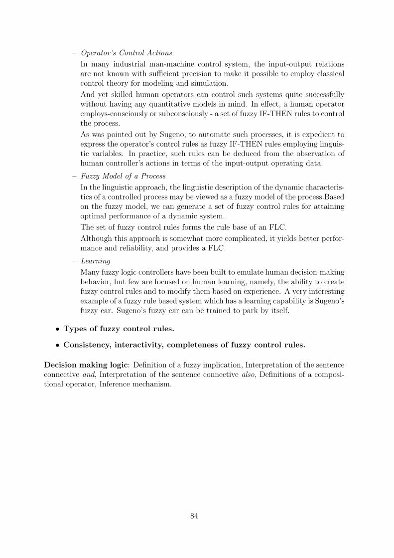
– Operator’s Control Actions
In many industrial man-machine control system, the input-output relationsare not known with sufficient precision to make it possible to employ classicalcontrol theory for modeling and simulation.
And yet skilled human operators can control such systems quite successfullywithout having any quantitative models in mind. In effect, a human operatoremploys-consciously or subconsciously - a set of fuzzy IF-THEN rules to controlthe process.
As was pointed out by Sugeno, to automate such processes, it is expedient toexpress the operator’s control rules as fuzzy IF-THEN rules employing linguis-tic variables. In practice, such rules can be deduced from the observation ofhuman controller’s actions in terms of the input-output operating data.
– Fuzzy Model of a Process
In the linguistic approach, the linguistic description of the dynamic characteris-tics of a controlled process may be viewed as a fuzzy model of the process.Basedon the fuzzy model, we can generate a set of fuzzy control rules for attainingoptimal performance of a dynamic system.
The set of fuzzy control rules forms the rule base of an FLC.
Although this approach is somewhat more complicated, it yields better perfor-mance and reliability, and provides a FLC.
– Learning
Many fuzzy logic controllers have been built to emulate human decision-makingbehavior, but few are focused on human learning, namely, the ability to createfuzzy control rules and to modify them based on experience. A very interestingexample of a fuzzy rule based system which has a learning capability is Sugeno’sfuzzy car. Sugeno’s fuzzy car can be trained to park by itself.
• Types of fuzzy control rules.
• Consistency, interactivity, completeness of fuzzy control rules.
Decision making logic: Definition of a fuzzy implication, Interpretation of the sentenceconnective and, Interpretation of the sentence connective also, Definitions of a composi-tional operator, Inference mechanism.
84
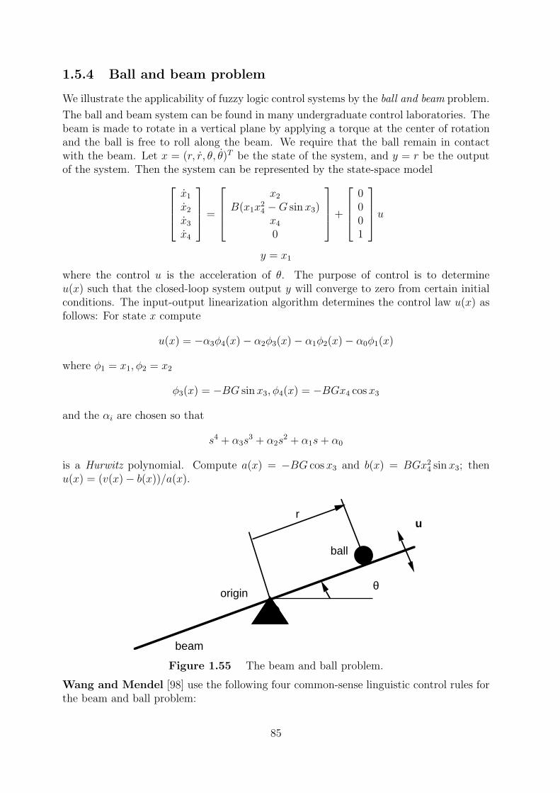
u
θ
r
origin
beam
ball
1.5.4 Ball and beam problem
We illustrate the applicability of fuzzy logic control systems by the ball and beam problem.
The ball and beam system can be found in many undergraduate control laboratories. Thebeam is made to rotate in a vertical plane by applying a torque at the center of rotationand the ball is free to roll along the beam. We require that the ball remain in contactwith the beam. Let x = (r, r, θ, θ)T be the state of the system, and y = r be the outputof the system. Then the system can be represented by the state-space model
x1
x2
x3
x4
=
x2
B(x1x24 −G sin x3)x4
0
+
0001
uy = x1
where the control u is the acceleration of θ. The purpose of control is to determineu(x) such that the closed-loop system output y will converge to zero from certain initialconditions. The input-output linearization algorithm determines the control law u(x) asfollows: For state x compute
u(x) = −α3φ4(x)− α2φ3(x)− α1φ2(x)− α0φ1(x)
where φ1 = x1, φ2 = x2
φ3(x) = −BG sin x3, φ4(x) = −BGx4 cos x3
and the αi are chosen so that
s4 + α3s3 + α2s
2 + α1s+ α0
is a Hurwitz polynomial. Compute a(x) = −BG cos x3 and b(x) = BGx24 sin x3; then
u(x) = (v(x)− b(x))/a(x).
Figure 1.55 The beam and ball problem.
Wang and Mendel [98] use the following four common-sense linguistic control rules forthe beam and ball problem:
85
<1: if x1 is ”positive” and x2 is ”near zero” and x3 is ”positive”and x4 is ”near zero” then ”u is negative”
<2: if x1 is ”positive” and x2 is ”near zero” and x3 is ”negative”and x4 is ”near zero” then ”u is positive big”
<3: if x1 is ”negative” and x2 is ”near zero” and x3 is ”positive”and x4 is ”near zero”then ”u is negative big”
<4: if x1 is ”negative” and x2 is ”near zero” and x3 is ”negative”and x4 is ”near zero” then ”u is positive”
where all fuzzy numbers have Gaussian membership function, e.g. the value ”near zero”of the linguistic variable x2 is defined by exp(−x2/2).
Figure 1.56 Gaussian membership function for ”near zero”
Using the Stone-Weierstrass theorem Wang [99] showed that fuzzy logic control systemsof the form
<i : if x is Ai and y is Bi then z is Ci, i = 1, . . . , n
with
• Gaussian membership functions
Ai(u) = exp
[−
1
2
(u− αi1βi1
)2],
Bi(v) = exp
[−
1
2
(v − αi2βi2
)2],
Ci(w) = exp
[−
1
2
(w − αi3βi3
)2],
• Singleton fuzzifier
fuzzifier(x) := x, fuzzifier(y) := y,
• Product fuzzy conjunction[Ai(u) and Bi(v)
]= Ai(u)Bi(v)
• Product fuzzy implication (Larsen implication)[Ai(u) and Bi(v)
]→ Ci(w) = Ai(u)Bi(v)Ci(w)
86
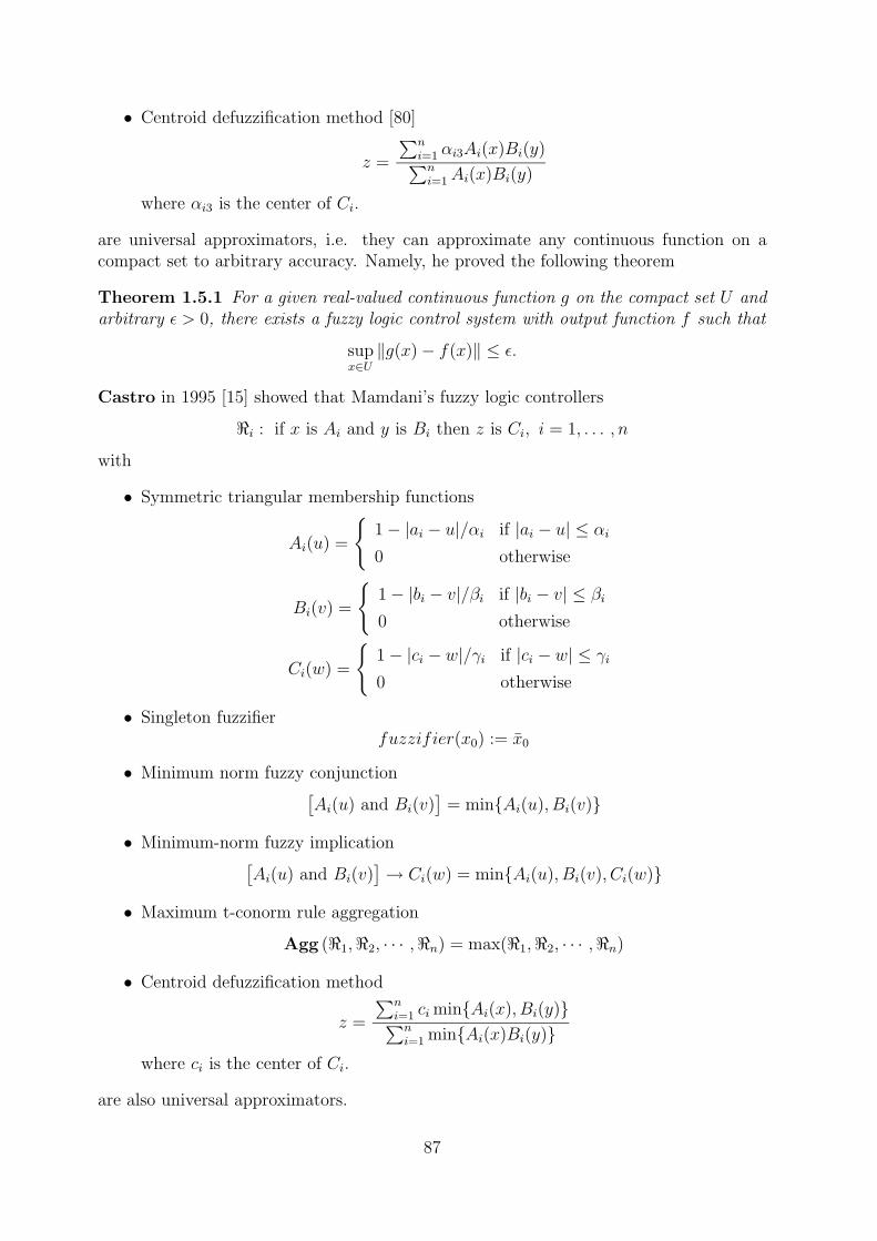
• Centroid defuzzification method [80]
z =
∑ni=1 αi3Ai(x)Bi(y)∑ni=1 Ai(x)Bi(y)
where αi3 is the center of Ci.
are universal approximators, i.e. they can approximate any continuous function on acompact set to arbitrary accuracy. Namely, he proved the following theorem
Theorem 1.5.1 For a given real-valued continuous function g on the compact set U andarbitrary ε > 0, there exists a fuzzy logic control system with output function f such that
supx∈U‖g(x)− f(x)‖ ≤ ε.
Castro in 1995 [15] showed that Mamdani’s fuzzy logic controllers
<i : if x is Ai and y is Bi then z is Ci, i = 1, . . . , n
with
• Symmetric triangular membership functions
Ai(u) =
{1− |ai − u|/αi if |ai − u| ≤ αi
0 otherwise
Bi(v) =
{1− |bi − v|/βi if |bi − v| ≤ βi
0 otherwise
Ci(w) =
{1− |ci − w|/γi if |ci − w| ≤ γi
0 otherwise
• Singleton fuzzifierfuzzifier(x0) := x0
• Minimum norm fuzzy conjunction[Ai(u) and Bi(v)
]= min{Ai(u), Bi(v)}
• Minimum-norm fuzzy implication[Ai(u) and Bi(v)
]→ Ci(w) = min{Ai(u), Bi(v), Ci(w)}
• Maximum t-conorm rule aggregation
Agg (<1,<2, · · · ,<n) = max(<1,<2, · · · ,<n)
• Centroid defuzzification method
z =
∑ni=1 ci min{Ai(x), Bi(y)}∑ni=1 min{Ai(x)Bi(y)}
where ci is the center of Ci.
are also universal approximators.
87
1.6 Aggregation in fuzzy system modeling
Many applications of fuzzy set theory involve the use of a fuzzy rule base to modelcomplex and perhaps ill-defined systems. These applications include fuzzy logic control,fuzzy expert systems and fuzzy systems modeling. Typical of these situations are set ofn rules of the form
<1 : if x is A1 then y is C1
also
<2 : if x is A2 then y is C2
also
· · · · · · · · · · · ·also
<n : if x is An then y is Cn
The fuzzy inference process consists of the following four step algorithm [107]:
• Determination of the relevance or matching of each rule to the current input value.
• Determination of the output of each rule as fuzzy subset of the output space. Weshall denote these individual rule outputs as Rj.
• Aggregation of the individual rule outputs to obtain the overall fuzzy system outputas fuzzy subset of the output space. We shall denote this overall output as R.
• Selection of some action based upon the output set.
Our purpose here is to investigate the requirements for the operations that can be usedto implement this reasoning process. We are particularly concerned with the third step,the rule output aggregation.
Let us look at the process for combining the individual rule outputs. A basic assumptionwe shall make is that the operation is pointwise and likewise. By pointwise we meanthat for every y, R(y) just depends upon Rj(y), j = 1, . . . , n. By likewise we mean thatthe process used to combine the Rj is the same for all of the y.
Let us denote the pointwise process we use to combine the individual rule outputs as
F (y) = Agg(R1(y), . . . , Rn(y))
In the above Agg is called the aggregation operator and the Rj(y) are the arguments.More generally, we can consider this as an operator
a = Agg(a1, . . . , an)
where the ai and a are values from the membership grade space, normally the unit interval.
Let us look at the minimal requirements associated with Agg. We first note that thecombination of of the individual rule outputs should be independent of the choice ofindexing of the rules. This implies that a required property that we must associate withth Agg operator is that of commutativity, the indexing of the arguments does not matter.
88
We note that the commutativity property allows to represent the arguments of the Aggoperator, as an unordered collection of possible duplicate values; such an object is a bag.
For an individual rule output, Rj, the membership grade Rj(y) indicates the degree orsterength to which this rule suggests that y is the appropriate solution. In particular iffor a pair of elements y′ and y′′ it is the case that
Ri(y′) ≥ Ri(y
′′),
then we are saying that rule j is preferring y′ as the system output over y′′. From this wecan reasonably conclude that if all rules prefer y′ over y′′ as output then the overall systemoutput should prefer y′ over y′′. This observation requires us to impose a monotonicitycondition on the Agg operation. In particular if
Rj(y′) ≥ Rj(y
′′),
for all j, thenR(y′) ≥ R(y′′).
There appears one other condition we need to impose upon the aggregation operator.Assume that there exists some rule whose firing level is zero. The implication of this isthat the rule provides no information regarding what should be the output of the system.It should not affect the final R. The first observation we can make is that whatever outputthis rule provides should not make make any distinction between the potential outputs.Thus, we see that the aggregation operator needs an identy element.
In summary, we see that the aggregation operator, Agg must satisfy three conditions:commutativity, monotonicity, must contain a fixed identity. These conditions are basedon the three requirements: that the indexing of the rules be unimportant, a positiveassociation between individual rule output and total system output, and non-firing rulesplay no role in the decision process.
These operators are called MICA (Monotonic Identity Commutative Aggregation) oper-ators [107]. MICA operators are the most general class for aggregation in fuzzy modeling.They include t-norms, t-conorms, averaging and compensatory operators.
Assume X is a set of elements. A bag drawn from X is any collection of elements whichis contained in X. A bag is different from a subset in that it allows multiple copies of thesame element. A bag is similar to a set in that the ordering of the elements in the bagdoes not matter. If A is a bag consisiting of a, b, c, d we denote this as A =< a, b, c, d >.Assume A and B are two bags. We denote the sum of the bags
C = A⊕B
where C is the bag consisting of the members of both A and B.
Example 1.6.1 Let A =< a, b, c, d > and B =< b, c, c > then
A⊕B =< a, b, c, d, b, c, c >
In the following we let Bag(X) indicate the set of all bags of the set X.
89
Definition 1.6.1 A functionF : Bag(X)→ X
is called a bag mapping from Bag(X) into the set X.
An important property of bag mappings are that they are commutative in the sense thatthe ordering of the elements does not matter.
Definition 1.6.2 Assume A =< a1, . . . , an > and B =< b1, . . . , bn > are two bags of thesame cardinality n. If the elements in A and B can be indexed in such way that ai ≥ bifor all i then we shall denote this A ≥ B.
Definition 1.6.3 (MICA operator) A bag mapping
M : Bag([0, 1])→ [0, 1]
is called MICA operator if it has the following two properties
• If A ≥ B then M(A) ≥M(B) (monotonicity)
• For every bag A there exists an element, u ∈ [0, 1], called the identity of A such thatif C = A⊕ < u > then M(C) = M(A) (identity)
Thus the MICA operator is endowed with two properties in addition to the inherentcommutativity of the bag operator, monotonicity and identity:
• The requirement of monotonicity appears natural for an aggregation operator inthat it provides some connection between the arguments and the aggregated value.
• The property of identity allows us to have the facility for aggregating data whichdoes not affect the overall result. This becomes useful for enabling us to includeimportances among other characteristics.
Fuzzy set theory provides a host of attractive aggregation connectives for integrating mem-bership values representing uncertain information. These connectives can be categorizedinto the following three classes union, intersection and compensation connectives.
Union produces a high output whenever any one of the input values representing degreesof satisfaction of different features or criteria is high. Intersection connectives produce ahigh output only when all of the inputs have high values. Compensative connectives havethe property that a higher degree of satisfaction of one of the criteria can compensate fora lower degree of satisfaction of another criteria to a certain extent.
In the sense, union connectives provide full compensation and intersection connectivesprovide no compensation.
90
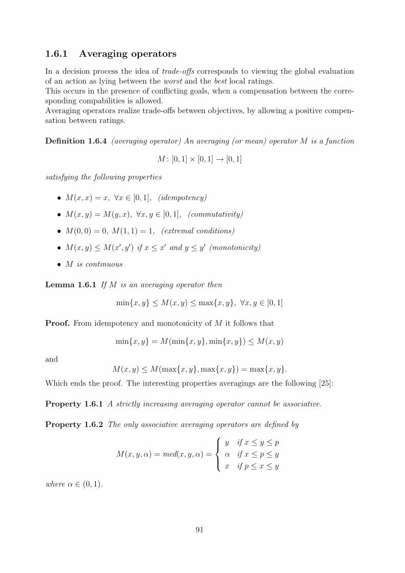
1.6.1 Averaging operators
In a decision process the idea of trade-offs corresponds to viewing the global evaluationof an action as lying between the worst and the best local ratings.This occurs in the presence of conflicting goals, when a compensation between the corre-sponding compabilities is allowed.Averaging operators realize trade-offs between objectives, by allowing a positive compen-sation between ratings.
Definition 1.6.4 (averaging operator) An averaging (or mean) operator M is a function
M : [0, 1]× [0, 1]→ [0, 1]
satisfying the following properties
• M(x, x) = x, ∀x ∈ [0, 1], (idempotency)
• M(x, y) = M(y, x), ∀x, y ∈ [0, 1], (commutativity)
• M(0, 0) = 0, M(1, 1) = 1, (extremal conditions)
• M(x, y) ≤M(x′, y′) if x ≤ x′ and y ≤ y′ (monotonicity)
• M is continuous
Lemma 1.6.1 If M is an averaging operator then
min{x, y} ≤M(x, y) ≤ max{x, y}, ∀x, y ∈ [0, 1]
Proof. From idempotency and monotonicity of M it follows that
min{x, y} = M(min{x, y},min{x, y}) ≤M(x, y)
andM(x, y) ≤M(max{x, y},max{x, y}) = max{x, y}.
Which ends the proof. The interesting properties averagings are the following [25]:
Property 1.6.1 A strictly increasing averaging operator cannot be associative.
Property 1.6.2 The only associative averaging operators are defined by
M(x, y, α) = med(x, y, α) =
y if x ≤ y ≤ p
α if x ≤ p ≤ y
x if p ≤ x ≤ y
where α ∈ (0, 1).
91
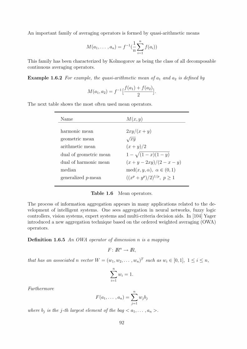
An important family of averaging operators is formed by quasi-arithmetic means
M(a1, . . . , an) = f−1(1
n
n∑i=1
f(ai))
This family has been characterized by Kolmogorov as being the class of all decomposablecontinuous averaging operators.
Example 1.6.2 For example, the quasi-arithmetic mean of a1 and a2 is defined by
M(a1, a2) = f−1[f(a1) + f(a2)
2
].
The next table shows the most often used mean operators.
Name M(x, y)
harmonic mean 2xy/(x+ y)
geometric mean√xy
arithmetic mean (x+ y)/2
dual of geometric mean 1−√
(1− x)(1− y)
dual of harmonic mean (x+ y − 2xy)/(2− x− y)
median med(x, y, α), α ∈ (0, 1)
generalized p-mean ((xp + yp)/2)1/p, p ≥ 1
Table 1.6 Mean operators.
The process of information aggregation appears in many applications related to the de-velopment of intelligent systems. One sees aggregation in neural networks, fuzzy logiccontrollers, vision systems, expert systems and multi-criteria decision aids. In [104] Yagerintroduced a new aggregation technique based on the ordered weighted averaging (OWA)operators.
Definition 1.6.5 An OWA operator of dimension n is a mapping
F : IRn → IR,
that has an associated n vector W = (w1, w2, . . . , wn)T such as wi ∈ [0, 1], 1 ≤ i ≤ n,
n∑i=1
wi = 1.
Furthermore
F (a1, . . . , an) =n∑j=1
wjbj
where bj is the j-th largest element of the bag < a1, . . . , an >.
92
Example 1.6.3 Assume W = (0.4, 0.3, 0.2, 0.1)T then
F (0.7, 1, 0.2, 0.6) = 0.4× 1 + 0.3× 0.7 + 0.2× 0.6 + 0.1× 0.2 = 0.75.
A fundamental aspect of this operator is the re-ordering step, in particular an aggregateai is not associated with a particular weight wi but rather a weight is associated with aparticular ordered position of aggregate.
When we view the OWA weights as a column vector we shall find it convenient to refer tothe weights with the low indices as weights at the top and those with the higher indiceswith weights at the bottom.
It is noted that different OWA operators are distinguished by their weighting function.In [104] Yager pointed out three important special cases of OWA aggregations:
• F ∗: In this case W = W ∗ = (1, 0 . . . , 0)T and
F ∗(a1, . . . , an) = maxi=1,... ,n
(ai),
• F∗: In this case W = W∗ = (0, 0 . . . , 1)T and
F∗(a1, . . . , an) = mini=1,... ,n
(ai),
• FA: In this case W = WA = (1/n, . . . , 1/n)T and
FA(a1, . . . , an) = 1/nn∑i=1
ai,
A number of important properties can be associated with the OWA operators. We shallnow discuss some of these.
For any OWA operator F
F∗(a1, . . . , an) ≤ F (a1, . . . , an) ≤ F ∗(a1, . . . , an).
Thus the upper an lower star OWA operator are its boundaries. From the above itbecomes clear that for any F
max(ai) ≤ F (a1, . . . , an) ≤ maxi(ai).
The OWA operator can be seen to be commutative. Let {a1, . . . , an} be a bag of aggregatesand let {d1, . . . , dn} be any permutation of the ai. Then for any OWA operator
F (a1, . . . , an) = F (d1, . . . , dn).
A third characteristic associated with these operators is monotonicity. Assume ai and ciare a collection of aggregates, i = 1, . . . , n such that for each i, ai ≥ ci. Then
F (a1, . . . , an) ≥ F (c1, c2, . . . , cn)
where F is some fixed weight OWA operator.
Another characteristic associated with these operators is idempotency. If ai = a for all ithen for any OWA operator
F (a1, . . . , an) = a.
From the above we can see the OWA operators have the basic properties associated withan averaging operator.
93
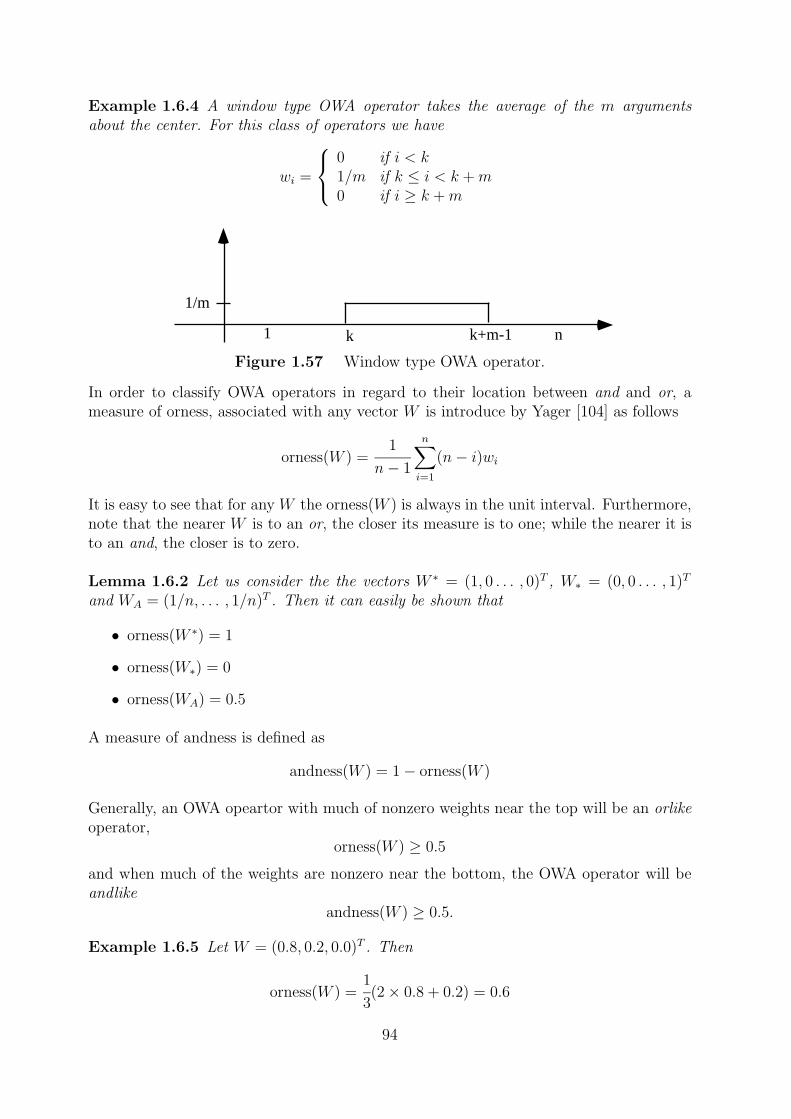
k k+m-11 n
1/m
Example 1.6.4 A window type OWA operator takes the average of the m argumentsabout the center. For this class of operators we have
wi =
0 if i < k1/m if k ≤ i < k +m0 if i ≥ k +m
Figure 1.57 Window type OWA operator.
In order to classify OWA operators in regard to their location between and and or, ameasure of orness, associated with any vector W is introduce by Yager [104] as follows
orness(W ) =1
n− 1
n∑i=1
(n− i)wi
It is easy to see that for any W the orness(W ) is always in the unit interval. Furthermore,note that the nearer W is to an or, the closer its measure is to one; while the nearer it isto an and, the closer is to zero.
Lemma 1.6.2 Let us consider the the vectors W ∗ = (1, 0 . . . , 0)T , W∗ = (0, 0 . . . , 1)T
and WA = (1/n, . . . , 1/n)T . Then it can easily be shown that
• orness(W ∗) = 1
• orness(W∗) = 0
• orness(WA) = 0.5
A measure of andness is defined as
andness(W ) = 1− orness(W )
Generally, an OWA opeartor with much of nonzero weights near the top will be an orlikeoperator,
orness(W ) ≥ 0.5
and when much of the weights are nonzero near the bottom, the OWA operator will beandlike
andness(W ) ≥ 0.5.
Example 1.6.5 Let W = (0.8, 0.2, 0.0)T . Then
orness(W ) =1
3(2× 0.8 + 0.2) = 0.6
94
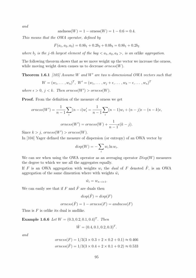
andandness(W ) = 1− orness(W ) = 1− 0.6 = 0.4.
This means that the OWA operator, defined by
F (a1, a2, a3) = 0.8b1 + 0.2b2 + 0.0b3 = 0.8b1 + 0.2b2
where bj is the j-th largest element of the bag < a1, a2, a3 >, is an orlike aggregation.
The following theorem shows that as we move weight up the vector we increase the orness,while moving weight down causes us to decrease orness(W ).
Theorem 1.6.1 [105] Assume W and W ′ are two n-dimensional OWA vectors such that
W = (w1, . . . , wn)T , W ′ = (w1, . . . , wj + ε, . . . , wk − ε, . . . , wn)T
where ε > 0, j < k. Then orness(W ′) > orness(W ).
Proof. From the definition of the measure of orness we get
orness(W ′) =1
n− 1
∑i
(n− i)w′i =1
n− 1
∑i
(n− 1)wi + (n− j)ε− (n− k)ε,
orness(W ′) = orness(W ) +1
n− 1ε(k − j).
Since k > j, orness(W ′) > orness(W ).
In [104] Yager defined the measure of dispersion (or entropy) of an OWA vector by
disp(W ) = −∑i
wi lnwi.
We can see when using the OWA operator as an averaging operator Disp(W ) measuresthe degree to which we use all the aggregates equally.
If F is an OWA aggregation with weights wi the dual of F denoted F , is an OWAaggregation of the same dimention where with weights wi
wi = wn−i+1.
We can easily see that if F and F are duals then
disp(F ) = disp(F )
orness(F ) = 1− orness(F ) = andness(F )
Thus is F is orlike its dual is andlike.
Example 1.6.6 Let W = (0.3, 0.2, 0.1, 0.4)T . Then
W = (0.4, 0.1, 0.2, 0.3)T .
andorness(F ) = 1/3(3× 0.3 + 2× 0.2 + 0.1) ≈ 0.466
orness(F ) = 1/3(3× 0.4 + 2× 0.1 + 0.2) ≈ 0.533
95
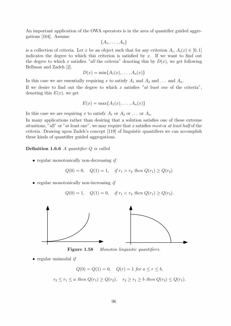
An important application of the OWA operators is in the area of quantifier guided aggre-gations [104]. Assume
{A1, . . . , An}is a collection of criteria. Let x be an object such that for any criterion Ai, Ai(x) ∈ [0, 1]indicates the degree to which this criterion is satisfied by x. If we want to find outthe degree to which x satisfies ”all the criteria” denoting this by D(x), we get followingBellman and Zadeh [2].
D(x) = min{A1(x), . . . , An(x)}In this case we are essentially requiring x to satisfy A1 and A2 and . . . and An.
If we desire to find out the degree to which x satisfies ”at least one of the criteria”,denoting this E(x), we get
E(x) = max{A1(x), . . . , An(x)}
In this case we are requiring x to satisfy A1 or A2 or . . . or An.
In many applications rather than desiring that a solution satisfies one of these extremesituations, ”all” or ”at least one”, we may require that x satisfies most or at least half of thecriteria. Drawing upon Zadeh’s concept [119] of linguistic quantifiers we can accomplishthese kinds of quantifier guided aggregations.
Definition 1.6.6 A quantifier Q is called
• regular monotonically non-decreasing if
Q(0) = 0, Q(1) = 1, if r1 > r2 then Q(r1) ≥ Q(r2).
• regular monotonically non-increasing if
Q(0) = 1, Q(1) = 0, if r1 < r2 then Q(r1) ≥ Q(r2).
Figure 1.58 Monoton linguistic quantifiers.
• regular unimodal if
Q(0) = Q(1) = 0, Q(r) = 1 for a ≤ r ≤ b,
r2 ≤ r1 ≤ a then Q(r1) ≥ Q(r2), r2 ≥ r1 ≥ b then Q(r2) ≤ Q(r1).
96
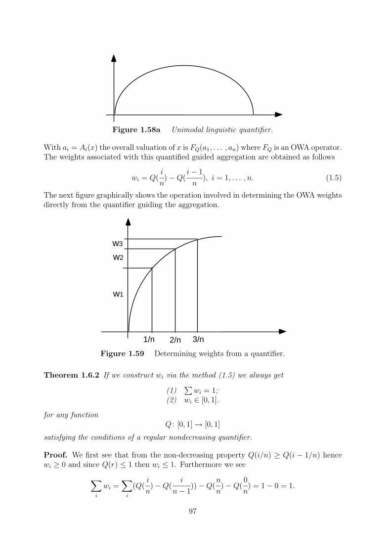
1/n 2/n 3/n
w1
w2
w3
Figure 1.58a Unimodal linguistic quantifier.
With ai = Ai(x) the overall valuation of x is FQ(a1, . . . , an) where FQ is an OWA operator.The weights associated with this quantified guided aggregation are obtained as follows
wi = Q(i
n)−Q(
i− 1
n), i = 1, . . . , n. (1.5)
The next figure graphically shows the operation involved in determining the OWA weightsdirectly from the quantifier guiding the aggregation.
Figure 1.59 Determining weights from a quantifier.
Theorem 1.6.2 If we construct wi via the method (1.5) we always get
(1)∑wi = 1;
(2) wi ∈ [0, 1].
for any functionQ : [0, 1]→ [0, 1]
satisfying the conditions of a regular nondecreasing quantifier.
Proof. We first see that from the non-decreasing property Q(i/n) ≥ Q(i − 1/n) hencewi ≥ 0 and since Q(r) ≤ 1 then wi ≤ 1. Furthermore we see∑
i
wi =∑i
(Q(i
n)−Q(
i
n− 1))−Q(
n
n)−Q(
0
n) = 1− 0 = 1.
97
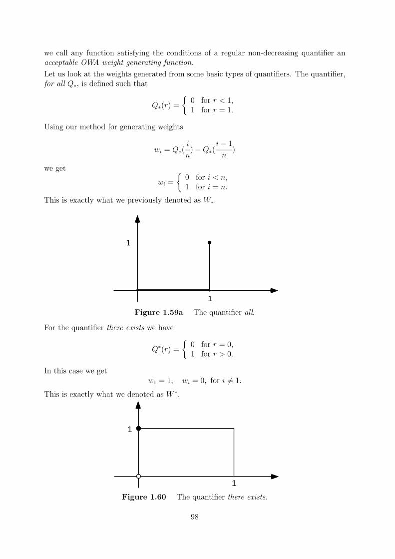
1
1
1
1
we call any function satisfying the conditions of a regular non-decreasing quantifier anacceptable OWA weight generating function.
Let us look at the weights generated from some basic types of quantifiers. The quantifier,for all Q∗, is defined such that
Q∗(r) =
{0 for r < 1,1 for r = 1.
Using our method for generating weights
wi = Q∗(i
n)−Q∗(
i− 1
n)
we get
wi =
{0 for i < n,1 for i = n.
This is exactly what we previously denoted as W∗.
Figure 1.59a The quantifier all.
For the quantifier there exists we have
Q∗(r) =
{0 for r = 0,1 for r > 0.
In this case we getw1 = 1, wi = 0, for i 6= 1.
This is exactly what we denoted as W ∗.
Figure 1.60 The quantifier there exists.
98
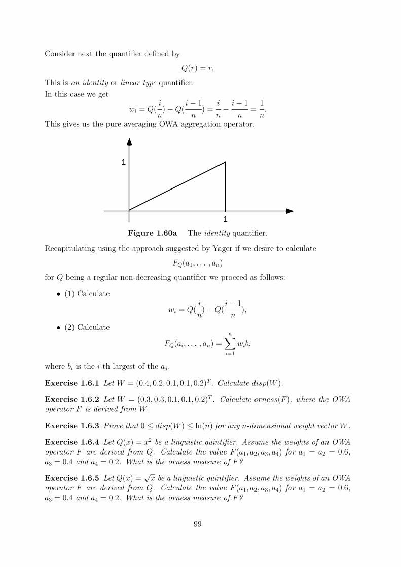
1
1
Consider next the quantifier defined by
Q(r) = r.
This is an identity or linear type quantifier.
In this case we get
wi = Q(i
n)−Q(
i− 1
n) =
i
n−i− 1
n=
1
n.
This gives us the pure averaging OWA aggregation operator.
Figure 1.60a The identity quantifier.
Recapitulating using the approach suggested by Yager if we desire to calculate
FQ(a1, . . . , an)
for Q being a regular non-decreasing quantifier we proceed as follows:
• (1) Calculate
wi = Q(i
n)−Q(
i− 1
n),
• (2) Calculate
FQ(ai, . . . , an) =n∑i=1
wibi
where bi is the i-th largest of the aj.
Exercise 1.6.1 Let W = (0.4, 0.2, 0.1, 0.1, 0.2)T . Calculate disp(W ).
Exercise 1.6.2 Let W = (0.3, 0.3, 0.1, 0.1, 0.2)T . Calculate orness(F ), where the OWAoperator F is derived from W .
Exercise 1.6.3 Prove that 0 ≤ disp(W ) ≤ ln(n) for any n-dimensional weight vector W .
Exercise 1.6.4 Let Q(x) = x2 be a linguistic quintifier. Assume the weights of an OWAoperator F are derived from Q. Calculate the value F (a1, a2, a3, a4) for a1 = a2 = 0.6,a3 = 0.4 and a4 = 0.2. What is the orness measure of F?
Exercise 1.6.5 Let Q(x) =√x be a linguistic quintifier. Assume the weights of an OWA
operator F are derived from Q. Calculate the value F (a1, a2, a3, a4) for a1 = a2 = 0.6,a3 = 0.4 and a4 = 0.2. What is the orness measure of F?
99
1.7 Fuzzy screening systems
In screening problems one usually starts with a large subset, X, of possible alternativesolutions. Each alternative is essentially represented by a minimal amount of informationsupporting its appropriateness as the best solution. This minimal amount of informa-tion provided by each alternative is used to help select a subset A of X to be furtherinvestigated.
Two prototypical examples of this kind of problem can be mentioned.
• Job selection problem. Here a large number of candidates, X, submit a resume,minimal information, to a job announcement. Based upon these resumes a smallsubset of X, A, are called in for interviews. These interviews, which provide moredetailed information, are the basis of selecting winning candidate from A.
• Proposal selection problem. Here a large class of candidates, X, submit pre-liminary proposals, minimal information. Based upon these preliminary proposals asmall subset of X, A, are requested to submit full detailed proposals. These detailedproposals are the basis of selecting winning candidate from A.
In the above examples the process of selecting the subset A, required to provide furtherinformation, is called a screening process. In [106] Yager suggests a technique, called fuzzyscreening system, for managing this screening process.
This kinds of screening problems described above besides being characterized as decisionmaking with minimal information general involve multiple participants in the selectionprocess. The people whose opinion must be considered in the selection process are calledexperts. Thus screening problems are a class of multiple expert decision problems. Inaddition each individual expert’s decision is based upon the use of multiple criteria. So wehave ME-MCDM (Multi Expert-Multi Criteria Decision Making) problem with minimalinformation.
The fact that we have minimal information associated with each of the alternatives com-plicates the problem because it limits the operations which can be performed in theaggregation processes needed to combine the multi-experts as well as multi-criteria. TheArrow impossibility theorem [1] is a reflection of this difficulty.
Yager [106] suggests an approach to the screening problem which allows for the requisiteaggregations but which respects the lack of detail provided by the information associatedwith each alternative. The technique only requires that preference information be ex-pressed in by elements draw from a scale that essentially only requires a linear ordering.This property allows the experts to provide information about satisfactions in the form ofa linguistic values such as high, medium, low. This ability to perform the necessary oper-ations will only requiring imprecise linguistic preference valuations will enable the expertsto comfortably use the kinds of minimally informative sources of information about theobjects described above. The fuzzy screening system is a two stage process.
• In the first stage, individual experts are asked to provide an evaluation of the al-ternatives. This evaluation consists of a rating for each alternative on each of thecriteria.
100
• In the second stage, the methodology introduced in [104] is used to aggregate theindividual experts evaluations to obtain an overall linguistic value for each object.This overall evaluation can then be used by the decision maker as an aid in theselection process.
The problem consists of three components.
• The first component is a collection
X = {X1, . . . , Xp}
of alternative solutions from amongst which we desire to select some subset to beinvestigated further.
• The second component is a group
A = {A1, . . . , Ar}
of experts or panelists whose opinion solicited in screening the alternatives.
• The third component is a collection
C = {C1, . . . , Cn}
of criteria which are considered relevant in the choice of the objects to be furtherconsidered.
For each alternative each expert is required to provided his opinion. In particular for eachalternative an expert is asked to evaluate how well that alternative satisfies each of thecriteria in the set C. These evaluations of alternative satisfaction to criteria will be givenin terms of elements from the following scale S:
Outstanding (OU) S7
Very High (VH) S6
High (H) S5
Medium (M) S4
Low S3
Very Low S2
None S1
The use of such a scale provides a natural ordering, Si > Sj if i > j and the maximumand minimum of any two scores re defined by
max(Si, Sj) = Si if Si ≥ Sj, min(Si, Sj) = Sj if Sj ≤ Si
We shall denote the max by ∨ and the min by ∧. Thus for an alternative an expertprovides a collection of n values
{P1, . . . ,Pn}where Pj is the rating of the alternative on the j-th criteria by the expert. Each Pj is anelement in the set of allowable scores S.
101
Assuming n = 5, a typical scoring for an alternative from one expert would be:
(medium, low, outstanding, very high, outstanding).
Independent of this evaluation of alternative satisfaction to criteria each expert mustassign a measure of importance to each of the criteria. An expert uses the same scale, S,to provide the importance associated with the criteria.
The next step in the process is to find the overall valuation for a alternative by a givenexpert.
In order to accomplish this overall evaluation, we use a methodology suggested by Yager[102]. A crucial aspect of this approach is the taking of the negation of the importancesas
Neg(Si) = Sq−i+1
For the scale that we are using, we see that the negation operation provides the following:
Neg(OU) = NNeg(V H) = V LNeg(H) = LNeg(M) = MNeg(L) = HNeg(V L) = V HNeg(N) = OU
Then the unit score of each alternative by each expert, denoted by U , is calculated asfollows
U = minj{Neg(Ij) ∨ Pj)} (1.6)
where Ij denotes the importance of the j-th critera.
In the above ∨ indicates the max operation. We note that (1.6) essentially is an andingof the criteria satisfactions modified by the importance of the criteria. The formula (1.6)can be seen as a measure of the degree to which an alternative satisfies the followingproposition:
All important criteria are satisfied.
Example 1.7.1 Consider some alternative with the following scores on five criteria
Criteria: C1 C2 C3 C4 C5
Importance: VH VH M L VL
Score: M L OU VH OU
In this case we have
U = min{Neg(V H) ∨M,Neg(V H) ∨ L,Neg(M) ∨OU,Neg(L) ∨ V H,Neg(V L) ∨OU}
= min{V L ∨M,V L ∨ L,M ∨OU,H ∨ V H, V H ∨OU} = min{M,L,OU, V H,OU} = L
102
The essential reason for the low performance of this object is that it performed low onthe second criteria which has a very high importance. The formulation of Equation 1.6can be seen as a generalization of a weighted averaging. Linguistically, this formulationis saying that
If a criterion is important then an should score well on it.
As a result of the first stage, we have for each alternative a collection of evaluations
{Xi1, Xi2, . . . , Xir}
where Xik is the unit evaluation of the i-th alternative by the k-th expert.
In the second stage the technique for combining the expert’s evaluation to obtain anoverall evaluation for each alternative is based upon the OWA operators.
The first step in this process is for the decision making body to provide an aggregationfunction which we shall denote as Q. This function can be seen as a generalization of theidea of how many experts it feels need to agree on an alternative for it to be acceptableto pass the screening process. In particular for each number i, where i runs from 1 to r,the decision making body must provide a value Q(i) indicating how satisfied it would bein passing an alternative that i of the experts where satisfied with. The values for Q(i)should be drawn from the scale S described above.
It should be noted that Q should have certain characteristics to make it rational:
• As more experts agree the decision maker’s satisfaction or confidence should increase
Q(i) ≥ Q(j), i > j.
• If all the experts are satisfied then his satisfaction should be the highest possible
Q(r) = Outstanding.
A number for special forms for Q are worth noting:
• If the decision making body requires all experts to support a alternative then weget
Q(i) = None for i > rQ(r) = Outstanding
• If the support of just one expert is enough to make a alternative worthy of consid-eration then
Q(i) = Outstanding for all i
• If at least m experts’ support is needed for consideration then
Q(i) = None i < jQ(i) = Outstanding i ≥ m
103
In order to define function Q, we introduce the operation Int[a] as returning the integervalue that is closest to the number a. In the following, we shall let q be the number ofpoints on the scale and r be the number of experts participating. This function whichemulates the average is denoted as QA(k) and is defined by
QA(k) = Sb(k)
where
b(k) = Int[1 + (k ×q − 1
r)]
for all k = 0, 1, . . . , r.
We note that whatever the values of q and r it is always the case that
QA(0) = S1, QA(r) = Sq
As an example of this function if r = 3 and q = 7 then
b(k) = Int[1 + (k ×6
3)] = Int[1 + 2k]
andQA(0) = S1, QA(1) = S3, QA(2) = S5, QA(3) = S7.
If r = 4 and q = 7 thenb(k) = Int[1 + k × 1.5]
andQA(0) = S1, QA(1) = S3, QA(2) = S4, QA(3) = S6, QA(4) = S7.
Having appropriately selected Q we are now in the position to use the OWA method foraggregating the expert opinions. Assume we have r experts, each of which has a unitevaluation for the i-th projected denoted Xik.
The first step in the OWA procedure is to order the Xik’s in descending order, thus weshall denote Bj as the j-th highest score among the experts unit scores for the project.To find the overall evaluation for the ith project, denoted Xi, we calculate
Xi = maxj{Q(j) ∧Bj}.
In order to appreciate the workings for this formulation we must realize that
• Bj can be seen as the worst of the j-th top scores.
• Q(j) ∧ Bj can be seen as an indication of how important the decision maker feelsthat the support of at least j experts is.
• The term Q(j) ∧Bj can be seen as a weighting of an objects j best scores, Bj, andthe decision maker requirement that j people support the project, Q(j).
• The max operator plays a role akin to the summation in the usual numeric averagingprocedure.
104
Example 1.7.2 Assume we have four experts each providing a unit evaluation for projecti obtained by the methodology discussed in the previous section.
Xi1 = MXi2 = HXi3 = HXi4 = V H
Reording these scores we getB1 = V HB2 = HB3 = HB4 = M
Furthermore, we shall assume that our decision making body chooses as its aggregationfunction the average like function QA. Then with r = 4 and scale cardinality q = 7, weobtain:
QA(1) = L (S3)QA(2) = M (S4)QA(3) = V H (S6)QA(4) = OU (S7)
We calculate the overall evaluation as
Xi = max{L ∧ V H,M ∧H, V H ∧H,OU ∧M}Xi = max{L,M,H,M}Xi = H
Thus the overall evaluation of this alternative is high.
Using the methodology suggested thus far we obtain for each alternative an overall ratingXi. These ratings allow us to obtain a evaluation of all the alternative without resortingto a numeric scale. The decision making body is now in the position to make its selectionof alternatives that are be passed through the screening process. A level S∗ from the scaleS is selected and all those alternatives that have an overall evaluation of S∗ or better arepassed to the next step in the decision process.
Exercise 1.7.1 Consider some alternative with the following scores on five criteria
Criteria: C1 C2 C3 C4 C5 C6
Importance: H VH M L VL M
Score: L VH OU VH OU M
Calculate the unit score of this alternative.
105
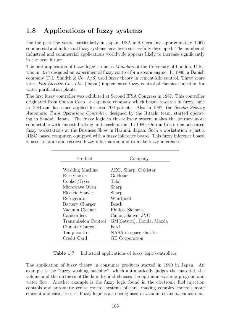
1.8 Applications of fuzzy systems
For the past few years, particularly in Japan, USA and Germany, approximately 1,000commercial and industrial fuzzy systems have been successfully developed. The number ofindustrial and commercial applications worldwide appears likely to increase significantlyin the near future.
The first application of fuzzy logic is due to Mamdani of the University of London, U.K.,who in 1974 designed an experimental fuzzy control for a steam engine. In 1980, a Danishcompany (F.L. Smidth & Co. A/S) used fuzzy theory in cement kiln control. Three yearslater, Fuji Electric Co., Ltd. (Japan) implemented fuzzy control of chemical injection forwater purification plants.
The first fuzzy controller was exhibited at Second IFSA Congress in 1987. This controlleroriginated from Omron Corp., a Japanese company which began research in fuzzy logicin 1984 and has since applied for over 700 patents. Also in 1987, the Sendai SubwayAutomatic Train Operations Controller, designed by the Hitachi team, started operat-ing in Sendai, Japan. The fuzzy logic in this subway system makes the journey morecomfortable with smooth braking and acceleration. In 1989, Omron Corp. demonstratedfuzzy workstations at the Business Show in Harumi, Japan. Such a workstation is just aRISC–based computer, equipped with a fuzzy inference board. This fuzzy inference boardis used to store and retrieve fuzzy information, and to make fuzzy inferences.
Product Company
Washing Machine AEG, Sharp, GoldstarRice Cooker GoldstarCooker/Fryer TefalMicrowave Oven SharpElectric Shaver SharpRefrigerator WhirlpoolBattery Charger BoschVacuum Cleaner Philips, SiemensCamcorders Canon, Sanyo, JVCTransmission Control GM(Saturn), Honda, MazdaClimate Control FordTemp control NASA in space shuttleCredit Card GE Corporation
Table 1.7 Industrial applications of fuzzy logic controllers.
The application of fuzzy theory in consumer products started in 1990 in Japan. Anexample is the ”fuzzy washing machine”, which automatically judges the material, thevolume and the dirtiness of the laundry and chooses the optimum washing program andwater flow. Another example is the fuzzy logic found in the electronic fuel injectioncontrols and automatic cruise control systems of cars, making complex controls moreefficient and easier to use. Fuzzy logic is also being used in vacuum cleaners, camcorders,
106
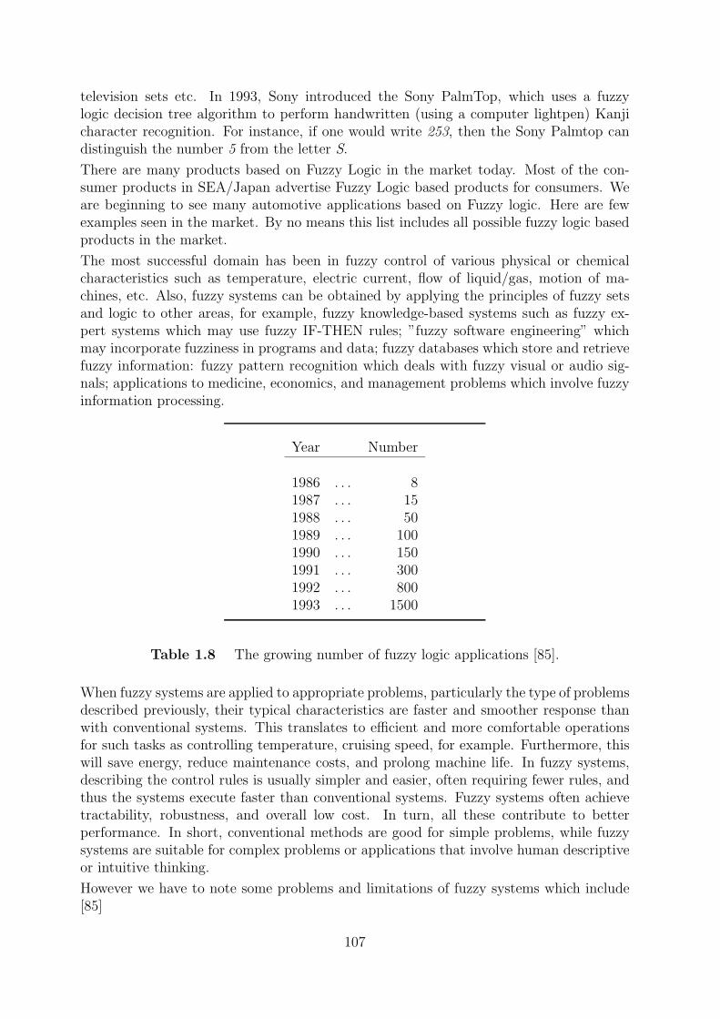
television sets etc. In 1993, Sony introduced the Sony PalmTop, which uses a fuzzylogic decision tree algorithm to perform handwritten (using a computer lightpen) Kanjicharacter recognition. For instance, if one would write 253, then the Sony Palmtop candistinguish the number 5 from the letter S.
There are many products based on Fuzzy Logic in the market today. Most of the con-sumer products in SEA/Japan advertise Fuzzy Logic based products for consumers. Weare beginning to see many automotive applications based on Fuzzy logic. Here are fewexamples seen in the market. By no means this list includes all possible fuzzy logic basedproducts in the market.
The most successful domain has been in fuzzy control of various physical or chemicalcharacteristics such as temperature, electric current, flow of liquid/gas, motion of ma-chines, etc. Also, fuzzy systems can be obtained by applying the principles of fuzzy setsand logic to other areas, for example, fuzzy knowledge-based systems such as fuzzy ex-pert systems which may use fuzzy IF-THEN rules; ”fuzzy software engineering” whichmay incorporate fuzziness in programs and data; fuzzy databases which store and retrievefuzzy information: fuzzy pattern recognition which deals with fuzzy visual or audio sig-nals; applications to medicine, economics, and management problems which involve fuzzyinformation processing.
Year Number
1986 . . . 81987 . . . 151988 . . . 501989 . . . 1001990 . . . 1501991 . . . 3001992 . . . 8001993 . . . 1500
Table 1.8 The growing number of fuzzy logic applications [85].
When fuzzy systems are applied to appropriate problems, particularly the type of problemsdescribed previously, their typical characteristics are faster and smoother response thanwith conventional systems. This translates to efficient and more comfortable operationsfor such tasks as controlling temperature, cruising speed, for example. Furthermore, thiswill save energy, reduce maintenance costs, and prolong machine life. In fuzzy systems,describing the control rules is usually simpler and easier, often requiring fewer rules, andthus the systems execute faster than conventional systems. Fuzzy systems often achievetractability, robustness, and overall low cost. In turn, all these contribute to betterperformance. In short, conventional methods are good for simple problems, while fuzzysystems are suitable for complex problems or applications that involve human descriptiveor intuitive thinking.
However we have to note some problems and limitations of fuzzy systems which include[85]
107
• Stability: a major issue for fuzzy control.
There is no theoretical guarantee that a general fuzzy system does not go chaoticand remains stable, although such a possibility appears to be extremely slim fromthe extensive experience.
• Learning capability: Fuzzy systems lack capabilities of learning and have no memoryas stated previously.
This is why hybrid systems, particularly neuro-fuzzy systems, are becoming moreand more popular for certain applications.
• Determining or tuning good membership functions and fuzzy rules are not alwayseasy.
Even after extensive testing, it is difficult to say how many membership functionsare really required. Questions such as why a particular fuzzy expert system needs somany rules or when can a developer stop adding more rules are not easy to answer.
• There exists a general misconception of the term ”fuzzy” as meaning imprecise orimperfect.
Many professionals think that fuzzy logic represents some magic without firm math-ematical foundation.
• Verification and validation of a fuzzy expert system generally requires extensivetesting with hardware in the loop.
Such luxury may not be affordable by all developers.
The basic steps for developing a fuzzy system are the following
• Determine whether a fuzzy system is a right choice for the problem. If the knowledgeabout the system behavior is described in approximate form or heuristic rules, thenfuzzy is suitable. Fuzzy logic can also be useful in understanding and simplifying theprocessing when the system behavior requires a complicated mathematical model.
• Identify inputs and outputs and their ranges. Range of sensor measurements typ-ically corresponds to the range of input variable, and the range of control actionsprovides the range of output variable.
• Define a primary membership function for each input and output parameter. Thenumber of membership functions required is a choice of the developer and dependson the system behavior.
• Construct a rule base. It is up to the designer to determine how many rules arenecessary.
• Verify that rule base output within its range for some sample inputs, and furthervalidate that this output is correct and proper according to the rule base for thegiven set of inputs.
Several studies show that fuzzy logic is applicable in Management Science (see e.g. [7]).
108
Bibliography
[1] K.J. Arrow, Social Choice and Individual Values (John Wiley & Sons, New York,1951).
[2] R.A.Bellman and L.A.Zadeh, Decision-making in a fuzzy environment, Manage-ment Sciences, Ser. B 17(1970) 141-164.
[3] D. Butnariu and E.P. Klement, Triangular Norm-Based Measures and Gameswith Fuzzy Coalitions (Kluwer, Dordrecht, 1993).
[4] D. Butnariu, E.P. Klement and S. Zafrany, On triangular norm-based proposi-tional fuzzy logics, Fuzzy Sets and Systems, 69(1995) 241-255.
[5] E. Canestrelli and S. Giove, Optimizing a quadratic function with fuzzy linearcoefficients, Control and Cybernetics, 20(1991) 25-36.
[6] E. Canestrelli and S. Giove, Bidimensional approach to fuzzy linear goal pro-gramming, in: M. Delgado, J. Kacprzyk, J.L. Verdegay and M.A. Vila eds.,Fuzzy Optimization (Physical Verlag, Heildelberg, 1994) 234-245.
[7] C. Carlsson, On the relevance of fuzzy sets in management science methodology,TIMS/Studies in the Management Sciences, 20(1984) 11-28.
[8] C. Carlsson, Fuzzy multiple criteria for decision support systems, in: M.M. Gup-ta, A. Kandel and J.B. Kiszka eds., Approximate Reasoning in Expert Systems(North-Holland, Amsterdam, 1985) 48-60.
[9] C. Carlsson and R.Fuller, Interdependence in fuzzy multiple objective program-ming, Fuzzy Sets and Systems 65(1994) 19-29.
[10] C. Carlsson and R. Fuller, Fuzzy if-then rules for modeling interdependenciesin FMOP problems, in: Proceedings of EUFIT’94 Conference, September 20-23,1994 Aachen, Germany (Verlag der Augustinus Buchhandlung, Aachen, 1994)1504-1508.
[11] C. Carlsson and R. Fuller, Interdependence in Multiple Criteria Decision Making,Technical Report, Institute for Advanced Management Systems Research, AboAkademi University, No. 1994/6.
[12] C. Carlsson and R.Fuller, Fuzzy reasoning for solving fuzzy multiple objectivelinear programs, in: R.Trappl ed., Cybernetics and Systems ’94, Proceedingsof the Twelfth European Meeting on Cybernetics and Systems Research (WorldScientific Publisher, London, 1994) 295-301.
109
[13] C. Carlsson and R.Fuller, Multiple Criteria Decision Making: The Case for In-terdependence, Computers & Operations Research 22(1995) 251-260.
[14] C. Carlsson and R. Fuller, On linear interdependences in MOP, in: Proceedingsof CIFT’95 Workshop, June 8-10, 1995, Trento, Italy, University of Trento, 199548-52.
[15] J.L. Castro, Fuzzy logic contollers are universal approximators, IEEE Transac-tions on Syst. Man Cybernet., 25(1995) 629-635.
[16] S.M. Chen, A weighted fuzzy reasoning akgorithm for medical diagnosis, DecisionSupport Systems, 11(1994) 37-43.
[17] E. Cox, The Fuzzy system Handbook. A Practitioner’s Guide to Building, Using,and Maintaining Fuzzy Systems (Academic Press, New York, 1994).
[18] M. Delgado, E. Trillas, J.L. Verdegay and M.A. Vila, The generalized ”modusponens” with linguistic labels, in: Proceedings of the Second International Con-ference on Fuzzy Logics andd Neural Network, IIzuka, Japan, 1990 725-729.
[19] M.Delgado, J. Kacprzyk, J.L.Verdegay and M.A.Vila eds., Fuzzy Optimization(Physical Verlag, Heildelberg, 1994).
[20] J. Dombi, A general class of fuzzy operators, the DeMorgan class of fuzzy opera-tors and fuziness measures induced by fuzzy operators, Fuzzy Sets and Systems,8(1982) 149-163.
[21] J. Dombi, Membership function as an evaluation, Fuzzy Sets and Systems,35(1990) 1-21.
[22] D. Driankov, H. Hellendoorn and M. Reinfrank, An Introduction to Fuzzy Control(Springer Verlag, Berlin, 1993).
[23] D. Dubois, R. Martin-Clouaire and H. Prade, Practical computation in fuzzylogic, in: M.M. Gupta and T. Yamakawa eds., Fuzzy Computing (Elsevier SciencePublishing, Amsterdam, 1988) 11-34.
[24] D. Dubois and H. Prade, Fuzzy Sets and Systems: Theory and Applications(Academic Press, London, 1980).
[25] D. Dubois and H. Prade, Criteria aggregation and ranking of alternatives inthe framework of fuzzy set theory, TIMS/Studies in the Management Sciences,20(1984) 209-240.
[26] D.Dubois and H.Prade, Possibility Theory (Plenum Press, New York,1988).
[27] D.Dubois, H.Prade and R.R Yager eds., Readings in Fuzzy Sets for IntelligentSystems (Morgan & Kaufmann, San Mateo, CA, 1993).
[28] G. W. Evans ed., Applications of Fuzzy Set Methodologies in Industrial Engi-neering (Elsevier, Amsterdam, 1989).
110
[29] M. Fedrizzi, J. Kacprzyk and S. Zadrozny, An interactive multi-user decisionsupport system for consensus reaching processes using fuzzy logic with linguisticquantifiers, Decision Support Systems, 4(1988) 313-327.
[30] M. Fedrizzi and L. Mich, Decision using production rules, in: Proc. of AnnualConference of the Operational Research Society of Italy, September 18-10, Rivadel Garda. Italy, 1991 118-121.
[31] M. Fedrizzi and R.Fuller, On stability in group decision support systems underfuzzy production rules, in: R.Trappl ed., Proceedings of the Eleventh EuropeanMeeting on Cybernetics and Systems Research (World Scientific Publisher, Lon-don, 1992) 471-478.
[32] M. Fedrizzi and R.Fuller, Stability in possibilistic linear programming problemswith continuous fuzzy number parameters, Fuzzy Sets and Systems, 47(1992)187-191.
[33] M. Fedrizzi, M, Fedrizzi and W. Ostasiewicz, Towards fuzzy modeling in eco-nomics, Fuzzy Sets and Systems (54)(1993) 259-268.
[34] M. Fedrizzi and R.Fuller, On stability in multiobjective possibilistic linear pro-grams, European Journal of Operational Reseach, 74(1994) 179-187.
[35] J.C. Fodor, A remark on constructing t-norms, Fuzzy Sets and Systems, 41(1991)195–199.
[36] J.C. Fodor, On fuzzy implication operators, Fuzzy Sets and Systems, 42(1991)293–300.
[37] J.C. Fodor, Strict preference relations based on weak t-norms, Fuzzy Sets andSystems, 43(1991) 327–336.
[38] J.C. Fodor, Traces of fuzzy binary relations, Fuzzy Sets and Systems, 50(1992)331–342.
[39] J.C. Fodor, An axiomatic approach to fuzzy preference modelling, Fuzzy Setsand Systems, 52(1992) 47–52.
[40] J.C. Fodor and M. Roubens, Aggregation and scoring procedures in multicriteriadecision making methods, in: Proceedings of the IEEE International Conferenceon Fuzzy Systems, San Diego, 1992 1261–1267.
[41] J.C. Fodor, Fuzzy connectives via matrix logic, Fuzzy Sets and Systems, 56(1993)67–77.
[42] J.C. Fodor, A new look at fuzzy connectives, Fuzzy Sets and System, 57(1993)141–148.
[43] J.C. Fodor and M. Roubens, Preference modelling and aggregation procedureswith valued binary relations, in: R. Lowen and M. Roubens eds., Fuzzy Logic:State of the Art (Kluwer, Dordrecht, 1993) 29–38.
111
[44] J.C. Fodor and M. Roubens, Fuzzy Preference Modelling and Multicriteria De-cision Aid (Kluwer Academic Publisher, Dordrecht, 1994).
[45] R. Fuller and T. Keresztfalvi, On Generalization of Nguyen’s theorem, FuzzySets and Systems, 41(1991) 371–374.
[46] R. Fuller, On Hamacher-sum of triangular fuzzy numbers, Fuzzy Sets and Sys-tems, 42(1991) 205-212.
[47] R. Fuller, Well-posed fuzzy extensions of ill-posed linear equality systems, FuzzySystems and Mathematics, 5(1991) 43-48.
[48] R. Fuller and B. Werners, The compositional rule of inference: introduction, the-oretical considerations, and exact calculation formulas, Working Paper, RWTHAachen, institut fur Wirtschaftswissenschaften, No.1991/7.
[49] R. Fuller, On law of large numbers for L-R fuzzy numbers, in: R. Lowen andM. Roubens eds., Proceedings of the Fourth IFSA Congress, Volume: Mathemat-ics, Brussels, 1991 74-77.
[50] R. Fuller and H.-J. Zimmermann, On Zadeh’s compositional rule of inference,in: R.Lowen and M.Roubens eds., Proceedings of the Fourth IFSA Congress,Volume: Artifical intelligence, Brussels, 1991 41-44.
[51] R. Fuller and H.-J. Zimmermann, On computation of the compositional rule ofinference under triangular norms, Fuzzy Sets and Systems, 51(1992) 267-275.
[52] R. Fuller and T. Keresztfalvi, t-Norm-based addition of fuzzy intervals, FuzzySets and Systems, 51(1992) 155-159.
[53] R. Fuller and B. Werners, The compositional rule of inference with several re-lations, in: B.Riecan and M.Duchon eds., Proceedings of the international Con-ference on Fuzzy Sets and its Applications, Liptovsky Mikulas, Czecho-Slovakia,February 17-21, 1992 (Math. Inst. Slovak Academy of Sciences, Bratislava, 1992)39–44.
[54] R. Fuller and H.-J.Zimmermann, Fuzzy reasoning for solving fuzzy mathe-matical programming problems, Working Paper, RWTH Aachen, institut furWirtschaftswissenschaften, No.1992/01.
[55] R. Fuller and H.-J. Zimmermann, On Zadeh’s compositional rule of inference,In: R.Lowen and M.Roubens eds., Fuzzy Logic: State of the Art, Theory andDecision Library, Series D (Kluwer Academic Publisher, Dordrecht, 1993) 193-200.
[56] R. Fuller and H.-J. Zimmermann, Fuzzy reasoning for solving fuzzy mathematicalprogramming problems, Fuzzy Sets and Systems 60(1993) 121-133.
[57] R. Fuller and E. Triesch, A note on law of large numbers for fuzzy variables,Fuzzy Sets and Systems, 55(1993).
112
[58] M.M. Gupta and D.H. Rao, On the principles of fuzzy neural networks, FuzzySets and Systems, 61(1994) 1-18.
[59] H. Hamacher, H.Leberling and H.-J.Zimmermann, Sensitivity analysis in fuzzylinear programming, Fuzzy Sets and Systems, 1(1978) 269-281.
[60] H. Hellendoorn, Closure properties of the compositional rule of inference, FuzzySets and Systems, 35(1990) 163-183.
[61] F. Herrera, M. Kovacs, and J. L. Verdegay, An optimum concept for fuzzifiedlinear programming problems: a parametric approach, Tatra Mountains Mathe-matical Publications, 1(1992) 57–64.
[62] F. Herrera, J. L. Verdegay, and M. Kovacs. A parametric approach for (g,p)-fuzzified linear programming problems, J. of Fuzzy Mathematics, 1(1993) 699–713.
[63] F. Herrera, M. Kovacs, and J. L. Verdegay, Optimality for fuzzified mathemat-ical programming problems: a parametric approach, Fuzzy Sets and Systems,54(1993) 279–285.
[64] J. Kacprzyk, Group decision making with a fuzzy linguistic majority, Fuzzy Setsand Systems, 18(1986) 105-118.
[65] O. Kaleva, Fuzzy differential equations, Fuzzy Sets and Systems, 24(1987) 301-317.
[66] A. Kaufmann and M.M. Gupta, Introduction to Fuzzy Arithmetic: Theory andApplications (Van Nostrand Reinhold, New York, 1991).
[67] T. Keresztfalvi, H. Rommelfanger, Multicriteria fuzzy optimization based onYager’s parameterized t-norm, Foundations of Comp. and Decision Sciences,16(1991) 99–110.
[68] T. Keresztfalvi, H. Rommelfanger, Fuzzy linear programming with t-norm basedextended addition, Operations Research Proceedings 1991 (Springer-Verlag,Berlin, Heidelberg, 1992) 492–499.
[69] L.T. Koczy, Fuzzy graphs in the evaluation and optimization of networks, FuzzySets and Systems, 46(1992) 307-319.
[70] L.T. Koczy and K.Hirota, A Fast algorithm for fuzzy inference by compact rules,in: L.A. Zadeh and J. Kacprzyk eds., Fuzzy Logic for the Management of Un-certainty (J. Wiley, New York, 1992) 297-317.
[71] L.T. Koczy, Approximate reasoning and control with sparse and/or inconsistentfuzzy rule bases, in: B. Reusch ed., Fuzzy Logic Theorie and Praxis, Springer,Berlin, 1993 42-65.
[72] L.T. Koczy and K. Hirota, Ordering, distance and Closeness of Fuzzy Sets, FuzzySets and Systems, 59(1993) 281-293.
113
[73] L.T. Koczy, A fast algorithm for fuzzy inference by compact rules, in: L.A. Zadehand J. Kacprzyk eds., Fuzzy Logic for the Management of Uncertainty (J. Wiley,New York, 1993) 297-317.
[74] B.Kosko, Neural networks and fuzzy systems, Prentice-Hall, New Jersey, 1992.
[75] B. Kosko, Fuzzy systems as universal approximators, in: Proc. IEEE 1992 Int.Conference Fuzzy Systems, San Diego, 1992 1153-1162.
[76] M.Kovacs and L.H. Tran, Algebraic structure of centered M -fuzzy numbers,Fuzzy Sets and Systems, 39(1991) 91–99.
[77] M. Kovacs, A stable embedding of ill-posed linear systems into fuzzy systems,Fuzzy Sets and Systems, 45(1992) 305–312.
[78] J.R.Layne, K.M.Passino and S.Yurkovich, Fuzzy learning control for antiskidbraking system, IEEE Transactions on Contr. Syst. Tech., 1(993) 122-129.
[79] C.-C. Lee, Fuzzy logic in control systems: Fuzzy logic controller - Part I, IEEETransactions on Syst., Man, Cybern., 20(1990) 419-435.
[80] C.-C. Lee, Fuzzy logic in control systems: Fuzzy logic controller - Part II, IEEETransactions on Syst., Man, Cybern., 20(1990) 404-418.
[81] E.H. Mamdani and S. Assilian, An experiment in linquistic synthesis with a fuzzylogic controller. International Journal of Man-Machine Studies 7(1975) 1-13.
[82] J.K. Mattila, On some logical points of fuzzy conditional decision making, FuzzySets and Systems, 20(1986) 137-145.
[83] G.F. Mauer, A fuzzy logic controller for an ABS braking system, IEEE Trans-actions on Fuzzy Systems, 3(1995) 381-388.
[84] D. McNeil and P, Freiberger, Fuzzy Logic (Simon and Schuster, New York, 1993).
[85] T. Munkata and Y.Jani, Fuzzy systems: An overview, Communications of ACM,37(1994) 69-76.
[86] C. V. Negoita, Fuzzy Systems (Abacus Press, Turnbridge-Wells, 1981).
[87] H.T. Nguyen, A note on the extension principle for fuzzy sets, Journal of Math-ematical Analysis and Applications, 64(1978) 369-380.
[88] S.A. Orlovsky, Calculus of Decomposable Properties. Fuzzy Sets and Decisions(Allerton Press, 1994).
[89] A.R. Ralescu, A note on rule representation in expert systems, InformationSciences, 38(1986) 193-203.
[90] H. Rommelfanger, Entscheiden bei Unscharfe: Fuzzy Decision Support-Systeme(Springer Verlag, Berlin, 1988).
114
[91] B.Schweizer and A.Sklar, Associative functions and abstract semigroups, Publ.Math. Debrecen, 10(1963) 69-81.
[92] T. Sudkamp, Similarity, interpolation, and fuzzy rule construction, Fuzzy Setsand Systems, 58(1993) 73-86.
[93] T.Takagi and M.Sugeno, Fuzzy identification of systems and its applications tomodeling and control, IEEE Trans. Syst. Man Cybernet., 1985, 116-132.
[94] M. Sugeno, Industrial Applications of Fuzzy Control (North Holland, Amster-dam, 1992).
[95] T. Tilli, Fuzzy Logik: Grundlagen, Anwendungen, Hard- und Software (Franzis-Verlag, Munchen, 1992).
[96] T. Tilli, Automatisierung mit Fuzzy Logik (Franzis-Verlag, Munchen, 1992).
[97] I.B. Turksen, Fuzzy normal forms, Fuzzy Sets and Systems, 69(1995) 319-346.
[98] L.-X. Wang and J.M. Mendel, Fuzzy basis functions, universal approximation,and orthogonal least-squares learning, IEEE Transactions on Neural Networks,3(1992) 807-814.
[99] L.-X. Wang, Fuzzy systems are universal approximators, in: Proc. IEEE 1992Int. Conference Fuzzy Systems, San Diego, 1992 1163-1170.
[100] S. Weber, A general concept of fuzzy connectives, negations, and implicationsbased on t-norms and t-conorms, Fuzzy Sets and Systems, 11(9183) 115-134.
[101] R.R. Yager, Fuzzy decision making using unequal objectives, Fuzzy Sets andSystems,1(1978) 87-95.
[102] R.R. Yager, A new methodology for ordinal multiple aspect decisions based onfuzzy sets, Decision Sciences 12(1981) 589-600.
[103] R.R. Yager ed., Fuzzy Sets and Applications. Selected Papers by L.A.Zadeh (JohnWiley & Sons, New York, 1987).
[104] R.R.Yager, Ordered weighted averaging aggregation operators in multi-criteriadecision making, IEEE Trans. on Systems, Man and Cybernetics, 18(1988) 183-190.
[105] R.R.Yager, Families of OWA operators, Fuzzy Sets and Systems, 59(1993) 125-148.
[106] R.R.Yager, Fuzzy Screening Systems, in: R.Lowen and M.Roubens eds., FuzzyLogic: State of the Art (Kluwer, Dordrecht, 1993) 251-261.
[107] R.R.Yager, Aggregation operators and fuzzy systems modeling, Fuzzy Sets andSystems, 67(1994) 129-145.
[108] R.R.Yager and D.Filev, Essentials of Fuzzy Modeling and Control (Wiley, NewYork, 1994).
115
[109] T. Yamakawa and K. Sasaki, Fuzzy memory device, in: Proceedings of 2nd IFSACongress, Tokyo, Japan, 1987 551-555.
[110] T. Yamakawa, Fuzzy controller hardware system, in: Proceedings of 2nd IFSACongress, Tokyo, Japan, 1987.
[111] T. Yamakawa, Fuzzy microprocessors - rule chip and defuzzifier chip, in: Inter-national Workshop on Fuzzy System Applications, Iizuka, Japan, 1988 51-52.
[112] J. Yen, R. Langari and L.A. Zadeh eds., Industrial Applications of Fuzzy Logicand Intelligent Systems (IEEE Press, New York, 1995).
[113] L.A. Zadeh, Fuzzy Sets, Information and Control, 8(1965) 338-353.
[114] L.A. Zadeh, Towards a theory of fuzzy systems, in: R.E. Kalman and N. DeClariseds., Aspects of Network and System Theory (Hort, Rinehart and Winston, NewYork, 1971) 469-490.
[115] L.A. Zadeh, Outline of a new approach to the analysis of complex systems and de-cision processes, IEEE Transanctins on Systems, Man and Cybernetics, 3(1973)28-44.
[116] L.A. Zadeh, Concept of a linguistic variable and its application to approximatereasoning, I, II, III, Information Sciences, 8(1975) 199-249, 301-357; 9(1975)43-80.
[117] L.A. Zadeh, Fuzzy sets as a basis for a theory of possibility, Fuzzy Sets andSystems, 1(1978) 3-28.
[118] L.A. Zadeh, A theory of approximate reasoning, In: J.Hayes, D.Michie andL.I.Mikulich eds., Machine Intelligence, Vol.9 (Halstead Press, New York, 1979)149-194.
[119] L.A. Zadeh, A computational theory of dispositions, Int. Journal of IntelligentSystems, 2(1987) 39-63.
[120] L.A. Zadeh, Knowledge representation in fuzzy logic, In: R.R.Yager and L.A.Zadeh eds., An introduction to fuzzy logic applications in intelligent systems(Kluwer Academic Publisher, Boston, 1992) 2-25.
[121] H.-J. Zimmermann and P. Zysno, Latent connectives in human decision making,Fuzzy Sets and Systems, 4(1980) 37-51.
[122] H.-J. Zimmermann, Fuzzy set theory and its applications (Kluwer, Dordrecht,1985).
[123] H.-J. Zimmermann, Fuzzy sets, Decision Making and Expert Systems (KluwerAcademic Publisher, Boston, 1987).
116

[124] H.-J.Zimmermann and B.Werners, Uncertainty representation in knowledge-based systems, in: A.S. Jovanovic, K.F. Kussmal, A.C. Lucia and P.P. Bonissoneeds., Proc. of an International Course on Expert Systems in Structural SafetyAssessment Stuttgart, October 2-4, 1989, (Springer-Verlag, Berlin, Heidelberg,1989) 151-166.
[125] H.-J.Zimmermann, Cognitive sciences, decision technology, and fuzzy sets, In-formation Sciences, 57-58(1991) 287-295.
117
Chapter 2
Artificial Neural Networks
2.1 The perceptron learning rule
Artificial neural systems can be considered as simplified mathematical models of brain-like systems and they function as parallel distributed computing networks. However,in contrast to conventional computers, which are programmed to perform specific task,most neural networks must be taught, or trained. They can learn new associations,new functional dependencies and new patterns. Although computers outperform bothbiological and artificial neural systems for tasks based on precise and fast arithmeticoperations, artificial neural systems represent the promising new generation of informationprocessing networks.
The study of brain-style computation has its roots over 50 years ago in the work ofMcCulloch and Pitts (1943) [19] and slightly later in Hebb’s famous Organization of Be-havior (1949) [11]. The early work in artificial intelligence was torn between those whobelieved that intelligent systems could best be built on computers modeled after brains,and those like Minsky and Papert (1969) [20] who believed that intelligence was funda-mentally symbol processing of the kind readily modeled on the von Neumann computer.For a variety of reasons, the symbol-processing approach became the dominant theme inArtifcial Intelligence in the 1970s. However, the 1980s showed a rebirth in interest inneural computing:
1982 Hopfield [14] provided the mathematical foundation for understanding the dynamicsof an important class of networks.
1984 Kohonen [16] developed unsupervised learning networks for feature mapping intoregular arrays of neurons.
1986 Rumelhart and McClelland [22] introduced the backpropagation learning algorithmfor complex, multilayer networks.
Beginning in 1986-87, many neural networks research programs were initiated. The listof applications that can be solved by neural networks has expanded from small test-sizeexamples to large practical tasks. Very-large-scale integrated neural network chips havebeen fabricated.
118
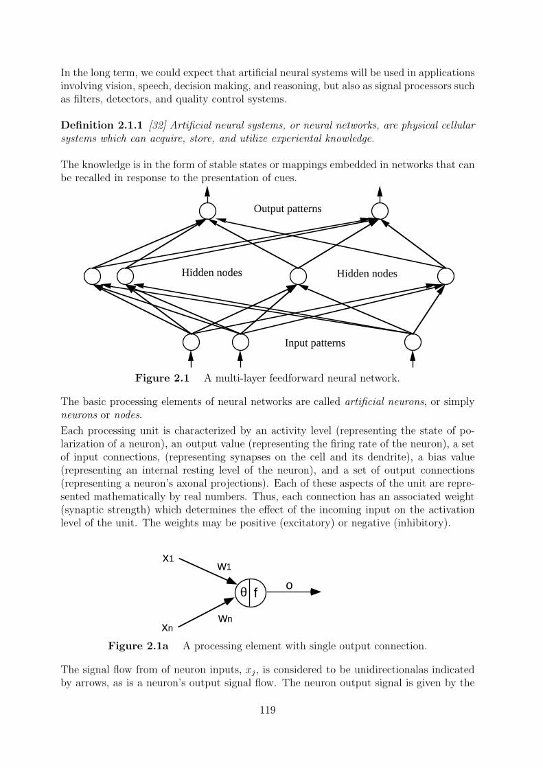
Output patterns
Hidden nodes
Input patterns
Hidden nodes
x1
xn
w1
wn
fθ ο
In the long term, we could expect that artificial neural systems will be used in applicationsinvolving vision, speech, decision making, and reasoning, but also as signal processors suchas filters, detectors, and quality control systems.
Definition 2.1.1 [32] Artificial neural systems, or neural networks, are physical cellularsystems which can acquire, store, and utilize experiental knowledge.
The knowledge is in the form of stable states or mappings embedded in networks that canbe recalled in response to the presentation of cues.
Figure 2.1 A multi-layer feedforward neural network.
The basic processing elements of neural networks are called artificial neurons, or simplyneurons or nodes.
Each processing unit is characterized by an activity level (representing the state of po-larization of a neuron), an output value (representing the firing rate of the neuron), a setof input connections, (representing synapses on the cell and its dendrite), a bias value(representing an internal resting level of the neuron), and a set of output connections(representing a neuron’s axonal projections). Each of these aspects of the unit are repre-sented mathematically by real numbers. Thus, each connection has an associated weight(synaptic strength) which determines the effect of the incoming input on the activationlevel of the unit. The weights may be positive (excitatory) or negative (inhibitory).
Figure 2.1a A processing element with single output connection.
The signal flow from of neuron inputs, xj, is considered to be unidirectionalas indicatedby arrows, as is a neuron’s output signal flow. The neuron output signal is given by the
119
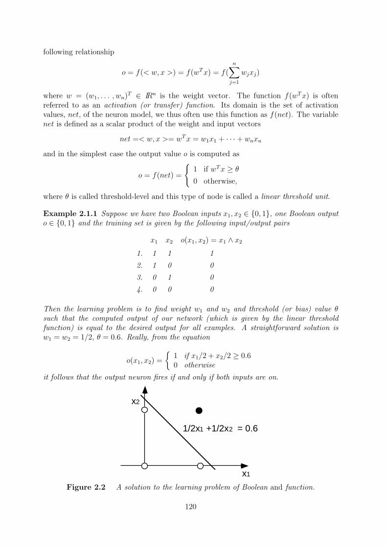
x1
x2
1/2x1 +1/2x2 = 0.6
following relationship
o = f(< w, x >) = f(wTx) = f(n∑j=1
wjxj)
where w = (w1, . . . , wn)T ∈ IRn is the weight vector. The function f(wTx) is oftenreferred to as an activation (or transfer) function. Its domain is the set of activationvalues, net, of the neuron model, we thus often use this function as f(net). The variablenet is defined as a scalar product of the weight and input vectors
net =< w, x >= wTx = w1x1 + · · ·+ wnxn
and in the simplest case the output value o is computed as
o = f(net) =
{1 if wTx ≥ θ
0 otherwise,
where θ is called threshold-level and this type of node is called a linear threshold unit.
Example 2.1.1 Suppose we have two Boolean inputs x1, x2 ∈ {0, 1}, one Boolean outputo ∈ {0, 1} and the training set is given by the following input/output pairs
x1 x2 o(x1, x2) = x1 ∧ x2
1. 1 1 1
2. 1 0 0
3. 0 1 0
4. 0 0 0
Then the learning problem is to find weight w1 and w2 and threshold (or bias) value θsuch that the computed output of our network (which is given by the linear thresholdfunction) is equal to the desired output for all examples. A straightforward solution isw1 = w2 = 1/2, θ = 0.6. Really, from the equation
o(x1, x2) =
{1 if x1/2 + x2/2 ≥ 0.60 otherwise
it follows that the output neuron fires if and only if both inputs are on.
Figure 2.2 A solution to the learning problem of Boolean and function.
120
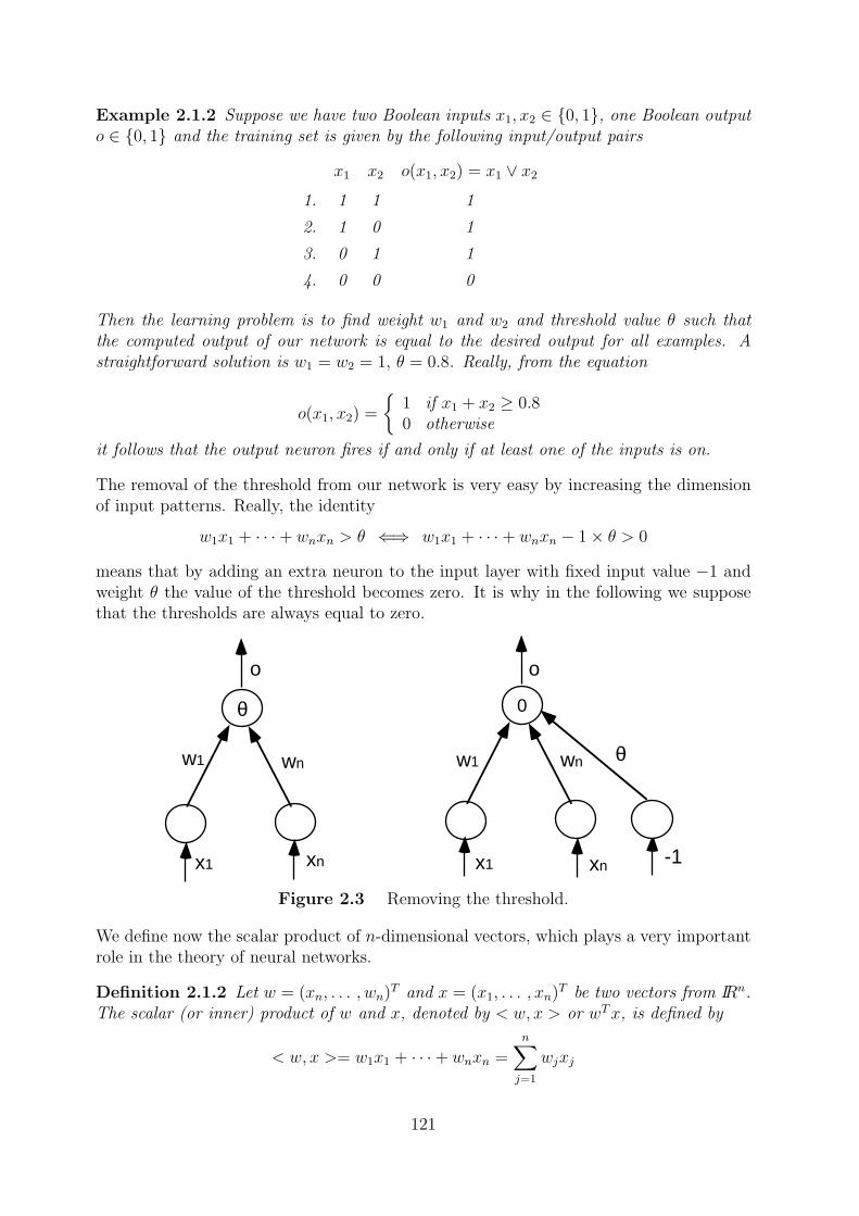
w1 wn
x1 xn
ο
θ
w1 wn
x1 xn
ο
θ
-1
0
Example 2.1.2 Suppose we have two Boolean inputs x1, x2 ∈ {0, 1}, one Boolean outputo ∈ {0, 1} and the training set is given by the following input/output pairs
x1 x2 o(x1, x2) = x1 ∨ x2
1. 1 1 1
2. 1 0 1
3. 0 1 1
4. 0 0 0
Then the learning problem is to find weight w1 and w2 and threshold value θ such thatthe computed output of our network is equal to the desired output for all examples. Astraightforward solution is w1 = w2 = 1, θ = 0.8. Really, from the equation
o(x1, x2) =
{1 if x1 + x2 ≥ 0.80 otherwise
it follows that the output neuron fires if and only if at least one of the inputs is on.
The removal of the threshold from our network is very easy by increasing the dimensionof input patterns. Really, the identity
w1x1 + · · ·+ wnxn > θ ⇐⇒ w1x1 + · · ·+ wnxn − 1× θ > 0
means that by adding an extra neuron to the input layer with fixed input value −1 andweight θ the value of the threshold becomes zero. It is why in the following we supposethat the thresholds are always equal to zero.
Figure 2.3 Removing the threshold.
We define now the scalar product of n-dimensional vectors, which plays a very importantrole in the theory of neural networks.
Definition 2.1.2 Let w = (xn, . . . , wn)T and x = (x1, . . . , xn)T be two vectors from IRn.The scalar (or inner) product of w and x, denoted by < w, x > or wTx, is defined by
< w, x >= w1x1 + · · ·+ wnxn =n∑j=1
wjxj
121
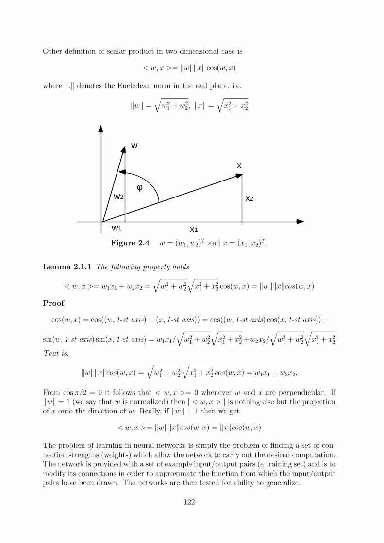
φ
w
x
x2
x1w1
w2
Other definition of scalar product in two dimensional case is
< w, x >= ‖w‖‖x‖ cos(w, x)
where ‖.‖ denotes the Eucledean norm in the real plane, i.e.
‖w‖ =√w2
1 + w22, ‖x‖ =
√x2
1 + x22
Figure 2.4 w = (w1, w2)T and x = (x1, x2)T .
Lemma 2.1.1 The following property holds
< w, x >= w1x1 + w2x2 =√w2
1 + w22
√x2
1 + x22 cos(w, x) = ‖w‖‖x‖cos(w, x)
Proof
cos(w, x) = cos((w, 1-st axis)− (x, 1-st axis)) = cos((w, 1-st axis) cos(x, 1-st axis))+
sin(w, 1-st axis) sin(x, 1-st axis) = w1x1/√w2
1 + w22
√x2
1 + x22 +w2x2/
√w2
1 + w22
√x2
1 + x22
That is,
‖w‖‖x‖cos(w, x) =√w2
1 + w22
√x2
1 + x22 cos(w, x) = w1x1 + w2x2.
From cosπ/2 = 0 it follows that < w, x >= 0 whenever w and x are perpendicular. If‖w‖ = 1 (we say that w is normalized) then | < w, x > | is nothing else but the projectionof x onto the direction of w. Really, if ‖w‖ = 1 then we get
< w, x >= ‖w‖‖x‖cos(w, x) = ‖x‖cos(w, x)
The problem of learning in neural networks is simply the problem of finding a set of con-nection strengths (weights) which allow the network to carry out the desired computation.The network is provided with a set of example input/output pairs (a training set) and is tomodify its connections in order to approximate the function from which the input/outputpairs have been drawn. The networks are then tested for ability to generalize.
122
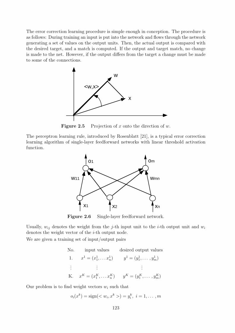
w
x
<w,x>
οm
x1 x2 xn
w11 wmn
ο1
The error correction learning procedure is simple enough in conception. The procedure isas follows: During training an input is put into the network and flows through the networkgenerating a set of values on the output units. Then, the actual output is compared withthe desired target, and a match is computed. If the output and target match, no changeis made to the net. However, if the output differs from the target a change must be madeto some of the connections.
Figure 2.5 Projection of x onto the direction of w.
The perceptron learning rule, introduced by Rosenblatt [21], is a typical error correctionlearning algorithm of single-layer feedforward networks with linear threshold activationfunction.
Figure 2.6 Single-layer feedforward network.
Usually, wij denotes the weight from the j-th input unit to the i-th output unit and widenotes the weight vector of the i-th output node.
We are given a training set of input/output pairs
No. input values desired output values
1. x1 = (x11, . . . x
1n) y1 = (y1
1, . . . , y1m)
......
...
K. xK = (xK1 , . . . xKn ) yK = (yK1 , . . . , y
Km)
Our problem is to find weight vectors wi such that
oi(xk) = sign(< wi, x
k >) = yki , i = 1, . . . ,m
123
for all training patterns k.
The activation function of the output nodes is linear threshold function of the form
oi(x) = sign(< wi, x >) =
{+1 if < wi, x >≥ 0−1 if < wi, x >< 0
and the weight adjustments in the perceptron learning method are performed by
wi := wi + η(yki − sign(< wi, xk >))xk, i = 1, . . . ,m
wij := wij + η(yki − sign(< wi, xk >))xkj , j = 1, . . . , n
where η > 0 is the learning rate.
From this equation it follows that if the desired output is equal to the computed output,yki = sign(< wi, x
k >), then the weight vector of the i-th output node remains unchanged,i.e. wi is adjusted if and only if the computed output, oi(x
k), is incorrect. The learningstops when all the weight vectors remain unchanged during a complete training cycle.
Consider now a single-layer network with one output node. Then the input componentsof the training patterns can be classified into two disjunct classes
C1 = {xk|yk = 1}, C2 = {xk|yk = −1}
i.e. x belongs to class C1 if there exists an input/output pair (x, 1), and x belongs to classC2 if there exists an input/output pair (x,−1).
Taking into consideration the definition of the activation function it is easy to see thatwe are searching for a weight vector w such that
< w, x >≥ 0 for each x ∈ C1, and < w, x >< 0 for each x ∈ C2.
If such vector exists then the problem is called linearly separable.
Summary 2.1.1 Perceptron learning algorithm.
Given are K training pairs arranged in the training set
(x1, y1), . . . , (xK , yK)
where xk = (xk1, . . . , xkn), yk = (yk1 , . . . , y
km), k = 1, . . . , K.
• Step 1 η > 0 is chosen
• Step 2 Weigts wi are initialized at small random values, the running error E is setto 0, k := 1
• Step 3 Training starts here. xk is presented, x := xk, y := yk and output o iscomputed
oi(x) = sign(< wi, x >), i = 1, . . . ,m
• Step 4 Weights are updated
wi := wi + η(yi − sign(< wi, x >))x, i = 1, . . . ,m
124
• Step 5 Cumulative cycle error is computed by adding the present error to E
E := E +1
2‖y − o‖2
• Step 6 If k < K then k := k + 1 and we continue the training by going back toStep 3, otherwise we go to Step 7
• Step 7 The training cycle is completed. For E = 0 terminate the training session.If E > 0 then E is set to 0, k := 1 and we initiate a new training cycle by going toStep 3
The following theorem shows that if the problem has solutions then the perceptron learn-ing algorithm will find one of them.
Theorem 2.1.1 (Convergence theorem) If the problem is linearly separable then the pro-gram will go to Step 3 only finetely many times.
Example 2.1.3 Illustration of the perceptron learning algorithm.
Consider the following training set
No. input values desired output value
1. x1 = (1, 0, 1)T -1
2. x2 = (0,−1,−1)T 1
3. x3 = (−1,−0.5,−1)T 1
The learning constant is assumed to be 0.1. The initial weight vector is w0 = (1,−1, 0)T .
Then the learning according to the perceptron learning rule progresses as follows.
Step 1 Input x1, desired output is -1:
< w0, x1 >= (1,−1, 0)
101
= 1
Correction in this step is needed since y1 = −1 6= sign(1). We thus obtain theupdated vector
w1 = w0 + 0.1(−1− 1)x1
Plugging in numerical values we obtain
w1 =
1−10
− 0.2
101
=
0.8−1−0.2
125
Step 2 Input is x2, desired output is 1. For the present w1 we compute the activation value
< w1, x2 >= (0.8,−1,−0.2)
0−1−1
= 1.2
Correction is not performed in this step since 1 = sign(1.2), so we let w2 := w1.
Step 3 Input is x3, desired output is 1.
< w2, x3 >= (0.8,−1,−0.2)
−1−0.5−1
= −0.1
Correction in this step is needed since y3 = 1 6= sign(−0.1). We thus obtain theupdated vector
w3 = w2 + 0.1(1 + 1)x3
Plugging in numerical values we obtain
w3 =
0.8−1−0.2
+ 0.2
−1−0.5−1
=
0.6−1.1−0.4
Step 4 Input x1, desired output is -1:
< w3, x1 >= (0.6,−1.1,−0.4)
101
= 0.2
Correction in this step is needed since y1 = −1 6= sign(0.2). We thus obtain theupdated vector
w4 = w3 + 0.1(−1− 1)x1
Plugging in numerical values we obtain
w4 =
0.6−1.1−0.4
− 0.2
101
=
0.4−1.1−0.6
Step 5 Input is x2, desired output is 1. For the present w4 we compute the activation value
< w4, x2 >= (0.4,−1.1,−0.6)
0−1−1
= 1.7
Correction is not performed in this step since 1 = sign(1.7), so we let w5 := w4.
Step 6 Input is x3, desired output is 1.
< w5, x3 >= (0.4,−1.1,−0.6)
−1−0.5−1
= 0.75
126
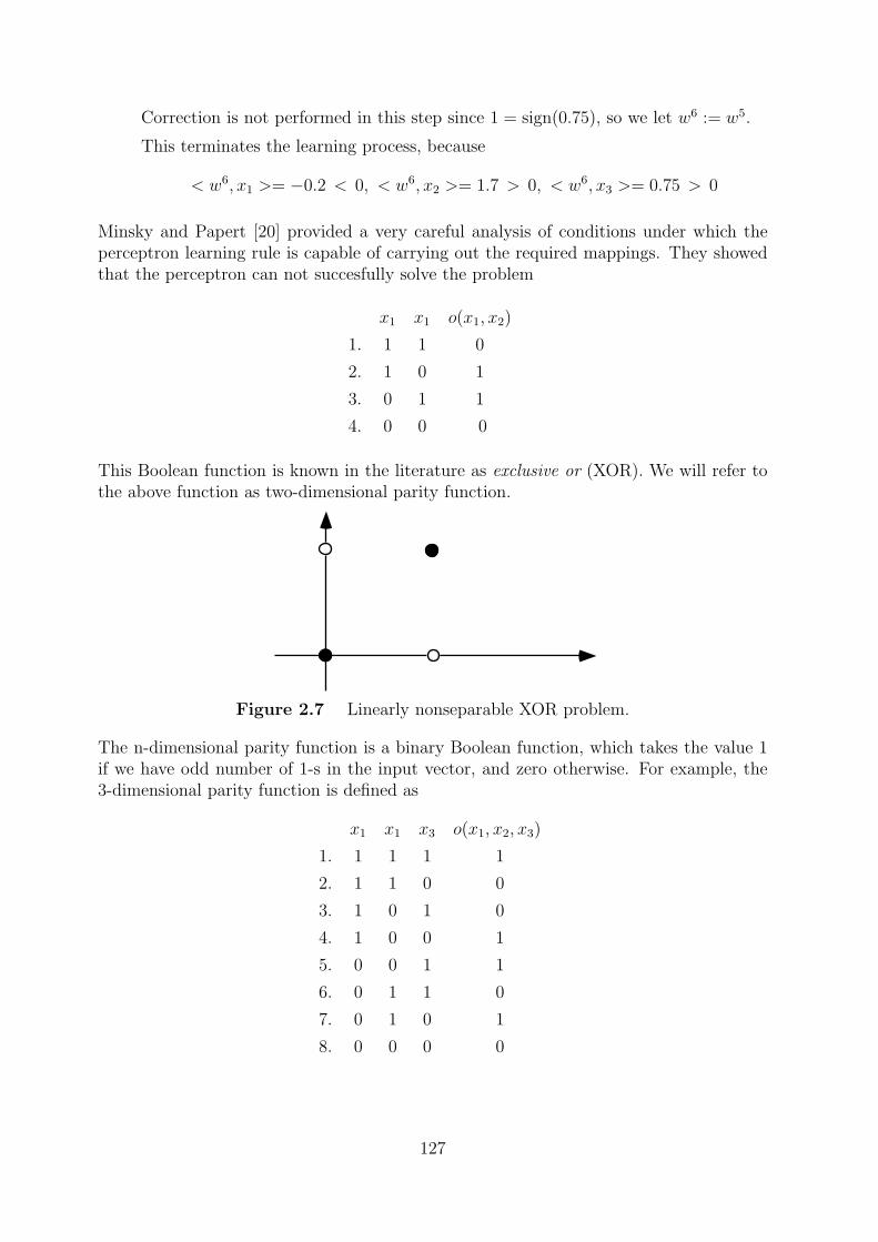
Correction is not performed in this step since 1 = sign(0.75), so we let w6 := w5.
This terminates the learning process, because
< w6, x1 >= −0.2 < 0, < w6, x2 >= 1.7 > 0, < w6, x3 >= 0.75 > 0
Minsky and Papert [20] provided a very careful analysis of conditions under which theperceptron learning rule is capable of carrying out the required mappings. They showedthat the perceptron can not succesfully solve the problem
x1 x1 o(x1, x2)
1. 1 1 0
2. 1 0 1
3. 0 1 1
4. 0 0 0
This Boolean function is known in the literature as exclusive or (XOR). We will refer tothe above function as two-dimensional parity function.
Figure 2.7 Linearly nonseparable XOR problem.
The n-dimensional parity function is a binary Boolean function, which takes the value 1if we have odd number of 1-s in the input vector, and zero otherwise. For example, the3-dimensional parity function is defined as
x1 x1 x3 o(x1, x2, x3)
1. 1 1 1 1
2. 1 1 0 0
3. 1 0 1 0
4. 1 0 0 1
5. 0 0 1 1
6. 0 1 1 0
7. 0 1 0 1
8. 0 0 0 0
127
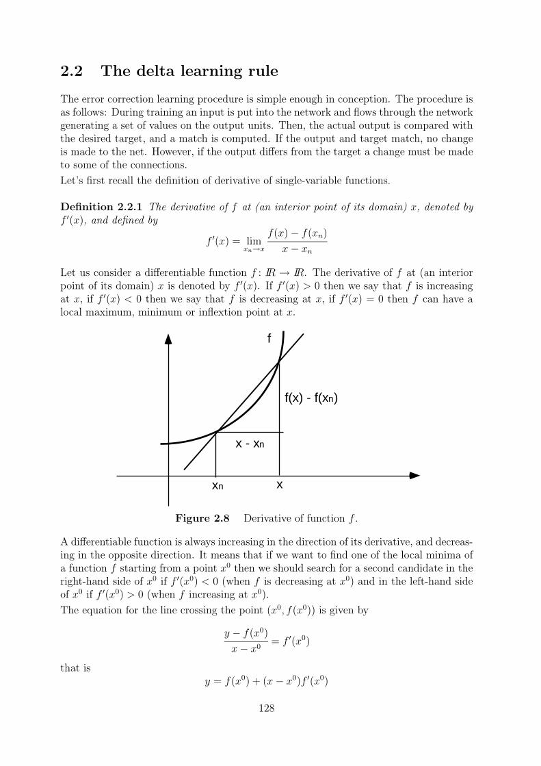
xxn
x - xn
f(x) - f(xn)
f
2.2 The delta learning rule
The error correction learning procedure is simple enough in conception. The procedure isas follows: During training an input is put into the network and flows through the networkgenerating a set of values on the output units. Then, the actual output is compared withthe desired target, and a match is computed. If the output and target match, no changeis made to the net. However, if the output differs from the target a change must be madeto some of the connections.
Let’s first recall the definition of derivative of single-variable functions.
Definition 2.2.1 The derivative of f at (an interior point of its domain) x, denoted byf ′(x), and defined by
f ′(x) = limxn→x
f(x)− f(xn)
x− xn
Let us consider a differentiable function f : IR → IR. The derivative of f at (an interiorpoint of its domain) x is denoted by f ′(x). If f ′(x) > 0 then we say that f is increasingat x, if f ′(x) < 0 then we say that f is decreasing at x, if f ′(x) = 0 then f can have alocal maximum, minimum or inflextion point at x.
Figure 2.8 Derivative of function f .
A differentiable function is always increasing in the direction of its derivative, and decreas-ing in the opposite direction. It means that if we want to find one of the local minima ofa function f starting from a point x0 then we should search for a second candidate in theright-hand side of x0 if f ′(x0) < 0 (when f is decreasing at x0) and in the left-hand sideof x0 if f ′(x0) > 0 (when f increasing at x0).
The equation for the line crossing the point (x0, f(x0)) is given by
y − f(x0)
x− x0= f ′(x0)
that isy = f(x0) + (x− x0)f ′(x0)
128
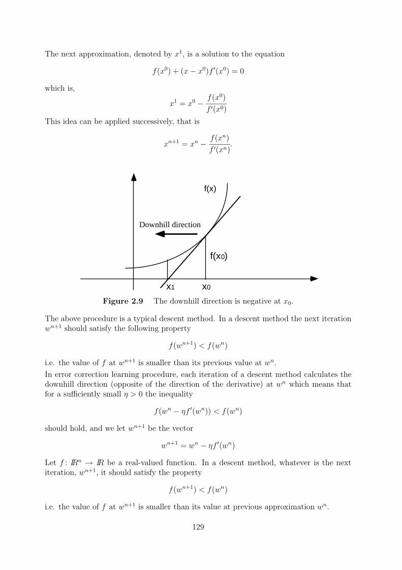
x0x1
f(x0)
f(x)
Downhill direction
The next approximation, denoted by x1, is a solution to the equation
f(x0) + (x− x0)f ′(x0) = 0
which is,
x1 = x0 −f(x0)
f ′(x0)
This idea can be applied successively, that is
xn+1 = xn −f(xn)
f ′(xn).
Figure 2.9 The downhill direction is negative at x0.
The above procedure is a typical descent method. In a descent method the next iterationwn+1 should satisfy the following property
f(wn+1) < f(wn)
i.e. the value of f at wn+1 is smaller than its previous value at wn.
In error correction learning procedure, each iteration of a descent method calculates thedownhill direction (opposite of the direction of the derivative) at wn which means thatfor a sufficiently small η > 0 the inequality
f(wn − ηf ′(wn)) < f(wn)
should hold, and we let wn+1 be the vector
wn+1 = wn − ηf ′(wn)
Let f : IRn → IR be a real-valued function. In a descent method, whatever is the nextiteration, wn+1, it should satisfy the property
f(wn+1) < f(wn)
i.e. the value of f at wn+1 is smaller than its value at previous approximation wn.
129
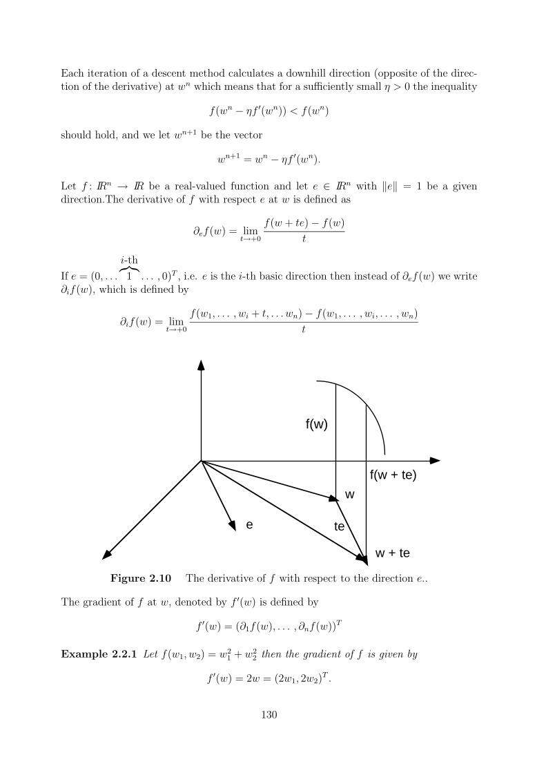
e te
f(w + te)
w
w + te
f(w)
Each iteration of a descent method calculates a downhill direction (opposite of the direc-tion of the derivative) at wn which means that for a sufficiently small η > 0 the inequality
f(wn − ηf ′(wn)) < f(wn)
should hold, and we let wn+1 be the vector
wn+1 = wn − ηf ′(wn).
Let f : IRn → IR be a real-valued function and let e ∈ IRn with ‖e‖ = 1 be a givendirection.The derivative of f with respect e at w is defined as
∂ef(w) = limt→+0
f(w + te)− f(w)
t
If e = (0, . . .
i-th︷︸︸︷1 . . . , 0)T , i.e. e is the i-th basic direction then instead of ∂ef(w) we write
∂if(w), which is defined by
∂if(w) = limt→+0
f(w1, . . . , wi + t, . . . wn)− f(w1, . . . , wi, . . . , wn)
t
Figure 2.10 The derivative of f with respect to the direction e..
The gradient of f at w, denoted by f ′(w) is defined by
f ′(w) = (∂1f(w), . . . , ∂nf(w))T
Example 2.2.1 Let f(w1, w2) = w21 + w2
2 then the gradient of f is given by
f ′(w) = 2w = (2w1, 2w2)T .
130
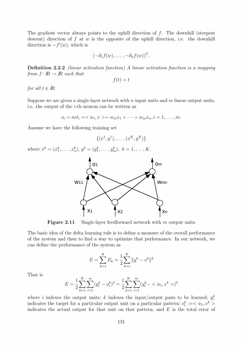
οm
x1 x2 xn
w11 wmn
ο1
The gradient vector always points to the uphill direction of f . The downhill (steepestdescent) direction of f at w is the opposite of the uphill direction, i.e. the downhilldirection is −f ′(w), which is
(−∂1f(w), . . . ,−∂nf(w))T .
Definition 2.2.2 (linear activation function) A linear activation function is a mappingfrom f : IR→ IR such that
f(t) = t
for all t ∈ IR.
Suppose we are given a single-layer network with n input units and m linear output units,i.e. the output of the i-th neuron can be written as
oi = neti =< wi, x >= wi1x1 + · · ·+ winxn, i = 1, . . . ,m.
Assume we have the following training set
{(x1, y1), . . . , (xK , yK)}
where xk = (xk1, . . . , xkn), yk = (yk1 , . . . , y
km), k = 1, . . . , K.
Figure 2.11 Single-layer feedforward network with m output units
The basic idea of the delta learning rule is to define a measure of the overall performanceof the system and then to find a way to optimize that performance. In our network, wecan define the performance of the system as
E =K∑k=1
Ek =1
2
K∑k=1
‖yk − ok‖2
That is
E =1
2
K∑k=1
m∑i=1
(yki − oki )2 =1
2
K∑k=1
m∑i=1
(yki− < wi, xk >)2
where i indexes the output units; k indexes the input/output pairs to be learned; ykiindicates the target for a particular output unit on a particular pattern; oki :=< wi, x
k >indicates the actual output for that unit on that pattern; and E is the total error of
131
the system. The goal, then, is to minimize this function. It turns out, if the outputfunctions are differentiable, that this problem has a simple solution: namely, we canassign a particular unit blame in proportion to the degree to which changes in that unit’sactivity lead to changes in the error. That is, we change the weights of the system inproportion to the derivative of the error with respect to the weights.
The rule for changing weights following presentation of input/output pair (xk, yk) is givenby the gradient descent method, i.e. we minimize the quadratic error function by usingthe following iteration process
wij := wij − η∂Ek
∂wij
where η > 0 is the learning rate.
Let us compute now the partial derivative of the error function Ek with respect to wij
∂Ek
∂wij=
∂Ek
∂netki
∂netki∂wij
= −(yki − oki )xkj
where netki = wi1xk1 + · · ·+ winx
kn.
That is,wij := wij + η(yki − oki )xkj
for j = 1, . . . , n.
Definition 2.2.3 The error signal term, denoted by δki and called delta, produced by thei-th output neuron is defined as
δki = −∂Ek
∂netki= (yki − oki )
For linear output units δki is nothing else but the difference between the desired and com-puted output values of the i-th neuron.
So the delta learning rule can be written as
wij := wij + ηδki xkj
for i = 1, . . . ,m and j = 1, . . . , n.
A key advantage of neural network systems is that these simple, yet powerful learningprocedures can be defined, allowing the systems to adapt to their environments.
The essential character of such networks is that they map similar input patterns to similaroutput patterns.
This characteristic is what allows these networks to make reasonable generalizations andperform reasonably on patterns that have never before been presented. The similarity ofpatterns in a connectionist system is determined by their overlap. The overlap in suchnetworks is determined outside the learning system itself whatever produces the patterns.The standard delta rule essentially implements gradient descent in sum-squared error forlinear activation functions.
It should be noted that the delta learning rule was introduced only recently for neuralnetwork training by McClelland and Rumelhart [22]. This rule parallels the discreteperceptron training rule. It also can be called the continuous perceptron training rule.
132
Summary 2.2.1 The delta learning rule with linear activation functions.
Given are K training pairs arranged in the training set
{(x1, y1), . . . , (xK , yK)}
where xk = (xk1, . . . , xkn) and yk = (yk1 , . . . , y
km), k = 1, . . . , K.
• Step 1 η > 0, Emax > 0 are chosen
• Step 2 Weights wij are initialized at small random values, k := 1, and the runningerror E is set to 0
• Step 3 Training starts here. Input xk is presented, x := xk, y := yk, and outputo = (o1, . . . , om)T is computed
o =< wi, x >= wTi x
for i = 1, . . . ,m.
• Step 4 Weights are updated
wij := wij + η(yi − oi)xj
• Step 5 Cumulative cycle error is computed by adding the present error to E
E := E +1
2‖y − o‖2
• Step 6 If k < K then k := k + 1 and we continue the training by going back toStep 3, otherwise we go to Step 7
• Step 7 The training cycle is completed. For E < Emax terminate the trainingsession. If E > Emax then E is set to 0 and we initiate a new training cycle by goingback to Step 3
133
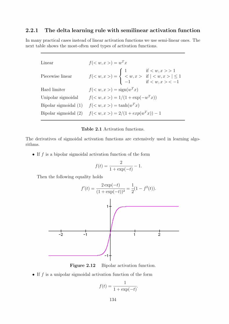
2.2.1 The delta learning rule with semilinear activation function
In many practical cases instead of linear activation functions we use semi-linear ones. Thenext table shows the most-often used types of activation functions.
Linear f(< w, x >) = wTx
Piecewise linear f(< w, x >) =
1 if < w, x >> 1< w, x > if | < w, x > | ≤ 1−1 if < w, x >< −1
Hard limiter f(< w, x >) = sign(wTx)
Unipolar sigmoidal f(< w, x >) = 1/(1 + exp(−wTx))
Bipolar sigmoidal (1) f(< w, x >) = tanh(wTx)
Bipolar sigmoidal (2) f(< w, x >) = 2/(1 + exp(wTx))− 1
Table 2.1 Activation functions.
The derivatives of sigmoidal activation functions are extensively used in learning algo-rithms.
• If f is a bipolar sigmoidal activation function of the form
f(t) =2
1 + exp(−t)− 1.
Then the following equality holds
f ′(t) =2 exp(−t)
(1 + exp(−t))2=
1
2(1− f 2(t)).
Figure 2.12 Bipolar activation function.
• If f is a unipolar sigmoidal activation function of the form
f(t) =1
1 + exp(−t).
134
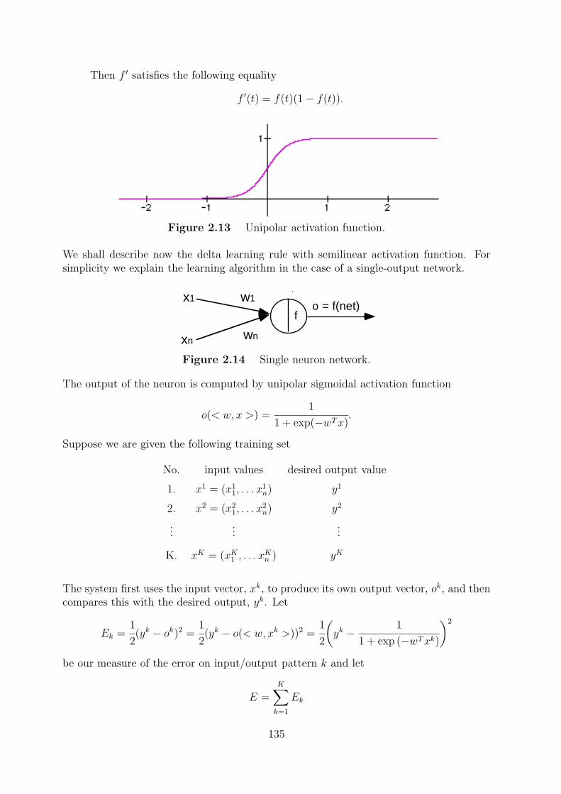
x1
xn
w1
wn
ο = f(net)f
Then f ′ satisfies the following equality
f ′(t) = f(t)(1− f(t)).
Figure 2.13 Unipolar activation function.
We shall describe now the delta learning rule with semilinear activation function. Forsimplicity we explain the learning algorithm in the case of a single-output network.
Figure 2.14 Single neuron network.
The output of the neuron is computed by unipolar sigmoidal activation function
o(< w, x >) =1
1 + exp(−wTx).
Suppose we are given the following training set
No. input values desired output value
1. x1 = (x11, . . . x
1n) y1
2. x2 = (x21, . . . x
2n) y2
......
...
K. xK = (xK1 , . . . xKn ) yK
The system first uses the input vector, xk, to produce its own output vector, ok, and thencompares this with the desired output, yk. Let
Ek =1
2(yk − ok)2 =
1
2(yk − o(< w, xk >))2 =
1
2
(yk −
1
1 + exp (−wTxk)
)2
be our measure of the error on input/output pattern k and let
E =K∑k=1
Ek
135
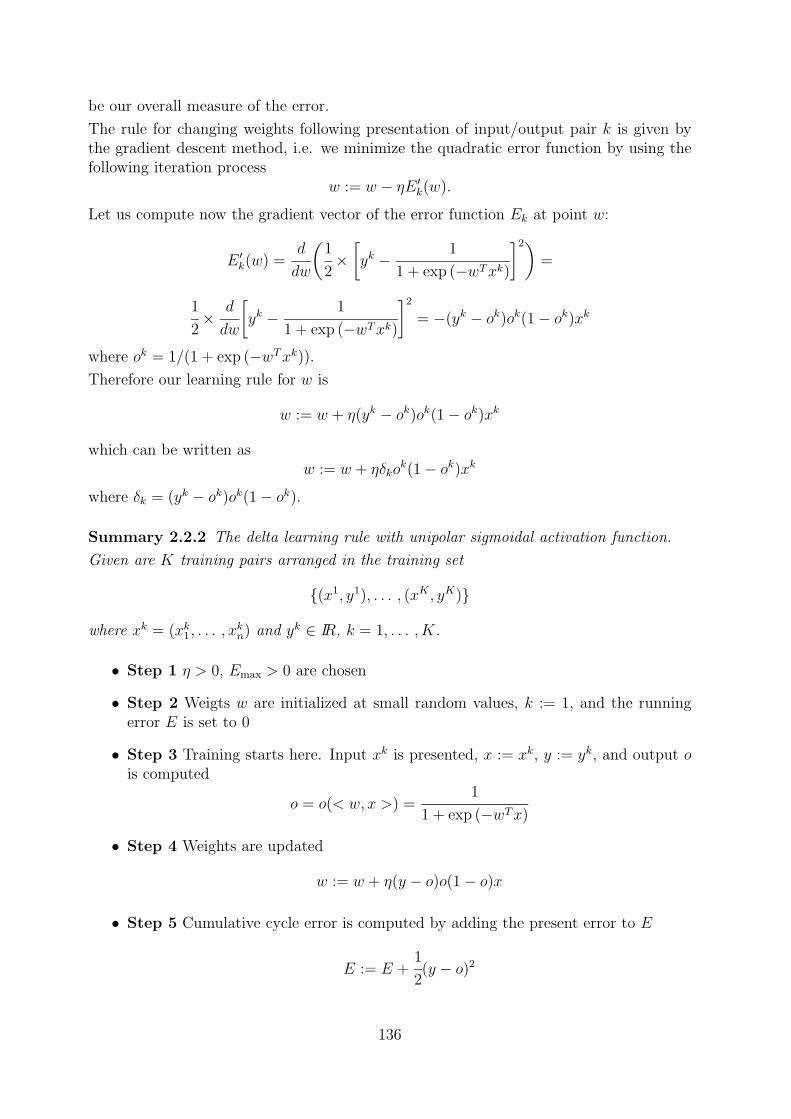
be our overall measure of the error.
The rule for changing weights following presentation of input/output pair k is given bythe gradient descent method, i.e. we minimize the quadratic error function by using thefollowing iteration process
w := w − ηE ′k(w).
Let us compute now the gradient vector of the error function Ek at point w:
E ′k(w) =d
dw
(1
2×[yk −
1
1 + exp (−wTxk)
]2)=
1
2×
d
dw
[yk −
1
1 + exp (−wTxk)
]2
= −(yk − ok)ok(1− ok)xk
where ok = 1/(1 + exp (−wTxk)).Therefore our learning rule for w is
w := w + η(yk − ok)ok(1− ok)xk
which can be written asw := w + ηδko
k(1− ok)xk
where δk = (yk − ok)ok(1− ok).
Summary 2.2.2 The delta learning rule with unipolar sigmoidal activation function.
Given are K training pairs arranged in the training set
{(x1, y1), . . . , (xK , yK)}
where xk = (xk1, . . . , xkn) and yk ∈ IR, k = 1, . . . , K.
• Step 1 η > 0, Emax > 0 are chosen
• Step 2 Weigts w are initialized at small random values, k := 1, and the runningerror E is set to 0
• Step 3 Training starts here. Input xk is presented, x := xk, y := yk, and output ois computed
o = o(< w, x >) =1
1 + exp (−wTx)
• Step 4 Weights are updated
w := w + η(y − o)o(1− o)x
• Step 5 Cumulative cycle error is computed by adding the present error to E
E := E +1
2(y − o)2
136
• Step 6 If k < K then k := k + 1 and we continue the training by going back toStep 3, otherwise we go to Step 7
• Step 7 The training cycle is completed. For E < Emax terminate the trainingsession. If E > Emax then E is set to 0 and we initiate a new training cycle by goingback to Step 3
In this case, without hidden units, the error surface is shaped like a bowl with only oneminimum, so gradient descent is guaranteed to find the best set of weights. With hiddenunits, however, it is not so obvious how to compute the derivatives, and the error surfaceis not concave upwards, so there is the danger of getting stuck in local minima.
We illustrate the delta learning rule with bipolar sigmoidal activation function f(t) =2/(1 + exp−t)− 1.
Example 2.2.2 The delta learning rule with bipolar sigmoidal activation function.
Given are K training pairs arranged in the training set
{(x1, y1), . . . , (xK , yK)}
where xk = (xk1, . . . , xkn) and yk ∈ IR, k = 1, . . . , K.
• Step 1 η > 0, Emax > 0 are chosen
• Step 2 Weigts w are initialized at small random values, k := 1, and the runningerror E is set to 0
• Step 3 Training starts here. Input xk is presented, x := xk, y := yk, and output ois computed
o = o(< w, x >) =2
1 + exp(−wTx)− 1
• Step 4 Weights are updated
w := w +1
2η(y − o)(1− o2)x
• Step 5 Cumulative cycle error is computed by adding the present error to E
E := E +1
2(y − o)2
• Step 6 If k < K then k := k + 1 and we continue the training by going back toStep 3, otherwise we go to Step 7
• Step 7 The training cycle is completed. For E < Emax terminate the trainingsession. If E > Emax then E is set to 0 and we initiate a new training cycle by goingback to Step 3
137
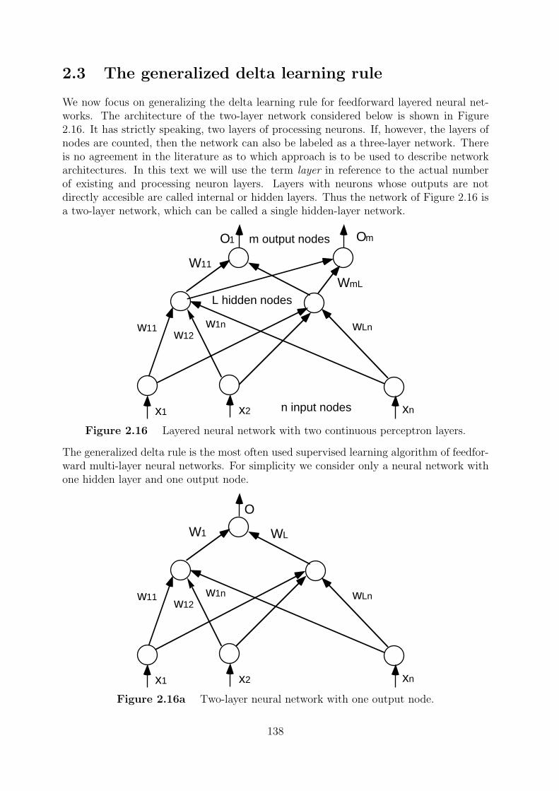
x1 x2 xn
w11 w12w1n wLn
L hidden nodes
W11
WmL
Ο1 Οmm output nodes
n input nodes
x1 x2 xn
w11 w12w1n wLn
W1 WL
Ο
2.3 The generalized delta learning rule
We now focus on generalizing the delta learning rule for feedforward layered neural net-works. The architecture of the two-layer network considered below is shown in Figure2.16. It has strictly speaking, two layers of processing neurons. If, however, the layers ofnodes are counted, then the network can also be labeled as a three-layer network. Thereis no agreement in the literature as to which approach is to be used to describe networkarchitectures. In this text we will use the term layer in reference to the actual numberof existing and processing neuron layers. Layers with neurons whose outputs are notdirectly accesible are called internal or hidden layers. Thus the network of Figure 2.16 isa two-layer network, which can be called a single hidden-layer network.
Figure 2.16 Layered neural network with two continuous perceptron layers.
The generalized delta rule is the most often used supervised learning algorithm of feedfor-ward multi-layer neural networks. For simplicity we consider only a neural network withone hidden layer and one output node.
Figure 2.16a Two-layer neural network with one output node.
138
The measure of the error on an input/output training pattern (xk, yk) is defined by
Ek(W,w) =1
2(yk −Ok)2
where Ok is the computed output and the overall measure of the error is
E(W,w) =K∑k=1
Ek(W,w).
If an input vector xk is presented to the network then it generates the following output
Ok =1
1 + exp(−W Tok)
where ok is the output vector of the hidden layer
okl =1
1 + exp(−wTl xk)and wl denotes the weight vector of the l-th hidden neuron, l = 1, . . . , L.
The rule for changing weights following presentation of input/output pair k is given bythe gradient descent method, i.e. we minimize the quadratic error function by using thefollowing iteration process
W := W − η∂Ek(W,w)
∂W,
wl := wl − η∂Ek(W,w)
∂wl,
for l = 1, . . . , L, and η > 0 is the learning rate.
By using the chain rule for derivatives of composed functions we get
∂Ek(W,w)
∂W=
1
2
∂
∂W
[yk −
1
1 + exp(−W Tok)
]2
= −(yk −Ok)Ok(1−Ok)ok
i.e. the rule for changing weights of the output unit is
W := W + η(yk −Ok)Ok(1−Ok)ok = W + ηδkok
that isWl := Wl + ηδko
kl ,
for l = 1, . . . , L, and we have used the notation δk = (yk −Ok)Ok(1−Ok).
Let us now compute the partial derivative of Ek with respect to wl
∂Ek(W,w)
∂wl= −Ok(1−Ok)Wlo
kl (1− okl )xk
i.e. the rule for changing weights of the hidden units is
wl := wl + ηδkWlokl (1− okl )xk, l = 1, . . . , L.
that iswlj := wlj + ηδkWlo
kl (1− okl )xkj , j = 1, . . . , n.
139
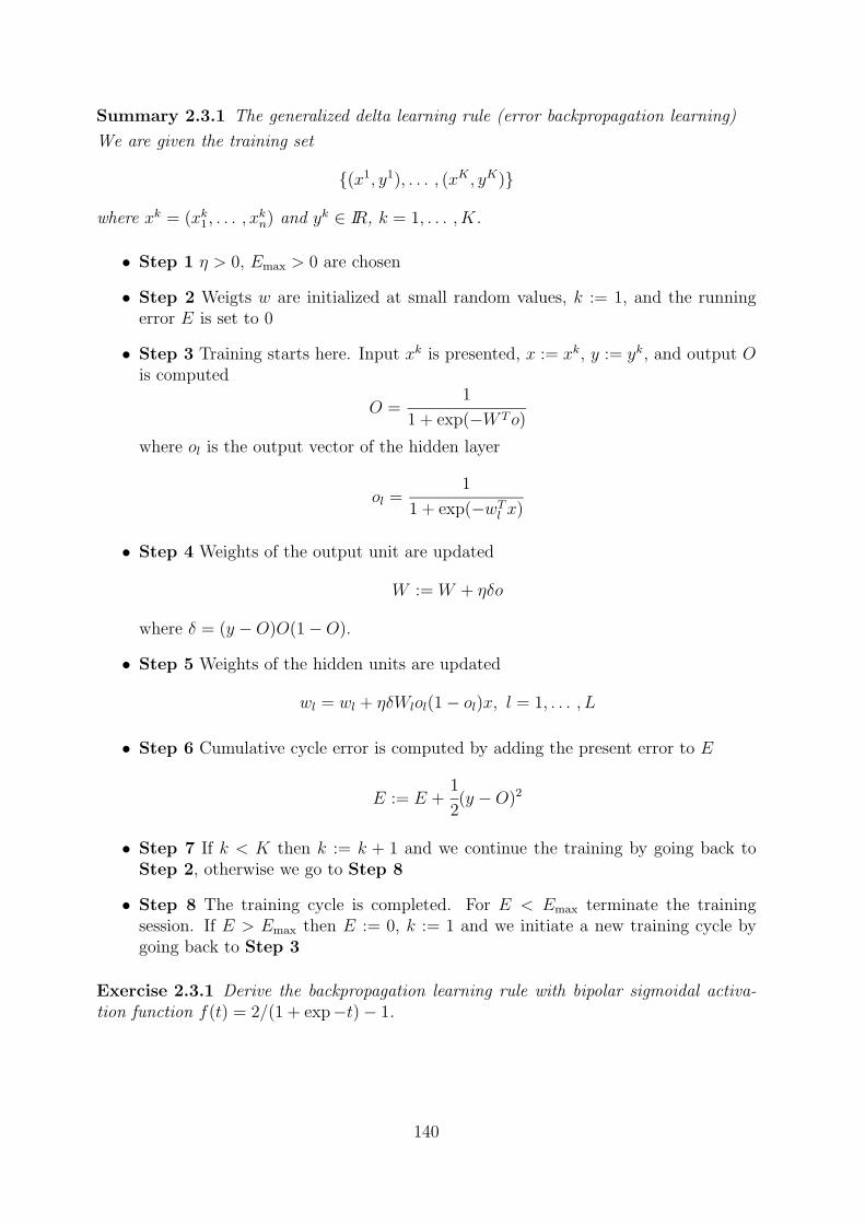
Summary 2.3.1 The generalized delta learning rule (error backpropagation learning)
We are given the training set
{(x1, y1), . . . , (xK , yK)}
where xk = (xk1, . . . , xkn) and yk ∈ IR, k = 1, . . . , K.
• Step 1 η > 0, Emax > 0 are chosen
• Step 2 Weigts w are initialized at small random values, k := 1, and the runningerror E is set to 0
• Step 3 Training starts here. Input xk is presented, x := xk, y := yk, and output Ois computed
O =1
1 + exp(−W To)
where ol is the output vector of the hidden layer
ol =1
1 + exp(−wTl x)
• Step 4 Weights of the output unit are updated
W := W + ηδo
where δ = (y −O)O(1−O).
• Step 5 Weights of the hidden units are updated
wl = wl + ηδWlol(1− ol)x, l = 1, . . . , L
• Step 6 Cumulative cycle error is computed by adding the present error to E
E := E +1
2(y −O)2
• Step 7 If k < K then k := k + 1 and we continue the training by going back toStep 2, otherwise we go to Step 8
• Step 8 The training cycle is completed. For E < Emax terminate the trainingsession. If E > Emax then E := 0, k := 1 and we initiate a new training cycle bygoing back to Step 3
Exercise 2.3.1 Derive the backpropagation learning rule with bipolar sigmoidal activa-tion function f(t) = 2/(1 + exp−t)− 1.
140
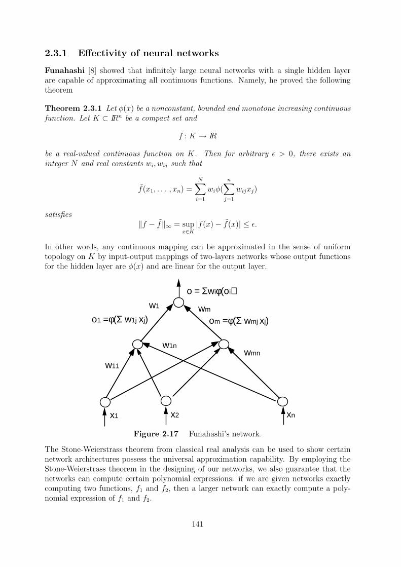
x1 x2 xn
w1 wm
w11
w1n
ο1 =φ(Σ w1j xj)
ο = Σwiφ(οi)
wmn
οm =φ(Σ wmj xj)
2.3.1 Effectivity of neural networks
Funahashi [8] showed that infinitely large neural networks with a single hidden layerare capable of approximating all continuous functions. Namely, he proved the followingtheorem
Theorem 2.3.1 Let φ(x) be a nonconstant, bounded and monotone increasing continuousfunction. Let K ⊂ IRn be a compact set and
f : K → IR
be a real-valued continuous function on K. Then for arbitrary ε > 0, there exists aninteger N and real constants wi, wij such that
f(x1, . . . , xn) =N∑i=1
wiφ(n∑j=1
wijxj)
satisfies‖f − f‖∞ = sup
x∈K|f(x)− f(x)| ≤ ε.
In other words, any continuous mapping can be approximated in the sense of uniformtopology on K by input-output mappings of two-layers networks whose output functionsfor the hidden layer are φ(x) and are linear for the output layer.
Figure 2.17 Funahashi’s network.
The Stone-Weierstrass theorem from classical real analysis can be used to show certainnetwork architectures possess the universal approximation capability. By employing theStone-Weierstrass theorem in the designing of our networks, we also guarantee that thenetworks can compute certain polynomial expressions: if we are given networks exactlycomputing two functions, f1 and f2, then a larger network can exactly compute a poly-nomial expression of f1 and f2.
141
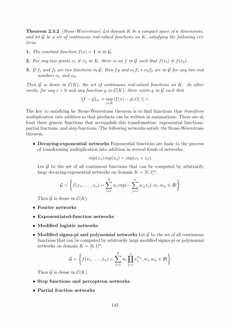
Theorem 2.3.2 (Stone-Weierstrass) Let domain K be a compact space of n dimensions,and let G be a set of continuous real-valued functions on K, satisfying the following cri-teria:
1. The constant function f(x) = 1 is in G.
2. For any two points x1 6= x2 in K, there is an f in G such that f(x1) 6= f(x2).
3. If f1 and f2 are two functions in G, then fg and α1f1 +α2f2 are in G for any two realnumbers α1 and α2.
Then G is dense in C(K), the set of continuous real-valued functions on K. In otherwords, for any ε > 0 and any function g in C(K), there exists g in G such that
‖f − g‖∞ = supx∈K|f(x)− g(x)| ≤ ε.
The key to satisfying he Stone-Weierstrass theorem is to find functions that transformmultiplication into addition so that products can be written as summations. There are atleast three generic functions that accomplish this transfomation: exponential functions,partial fractions, and step functions. The following networks satisfy the Stone-Weierstrasstheorem.
• Decaying-exponential networks Exponential functions are basic to the processof transforming multiplication into addition in several kinds of networks:
exp(x1) exp(x2) = exp(x1 + x2).
Let G be the set of all continuous functions that can be computed by arbitrarilylarge decaying-exponential networks on domain K = [0, 1]n:
G =
{f(x1, . . . , xn) =
N∑i=1
wi exp(−n∑j=1
wijxj), wi, wij ∈ IR}.
Then G is dense in C(K)
• Fourier networks
• Exponentiated-function networks
• Modified logistic networks
• Modified sigma-pi and polynomial networks Let G be the set of all continuousfunctions that can be computed by arbitrarily large modified sigma-pi or polynomialnetworks on domain K = [0, 1]n:
G =
{f(x1, . . . , xn) =
N∑i=1
wi
n∏j=1
xwijj , wi, wij ∈ IR
}.
Then G is dense in C(K).
• Step functions and perceptron networks
• Partial fraction networks
142
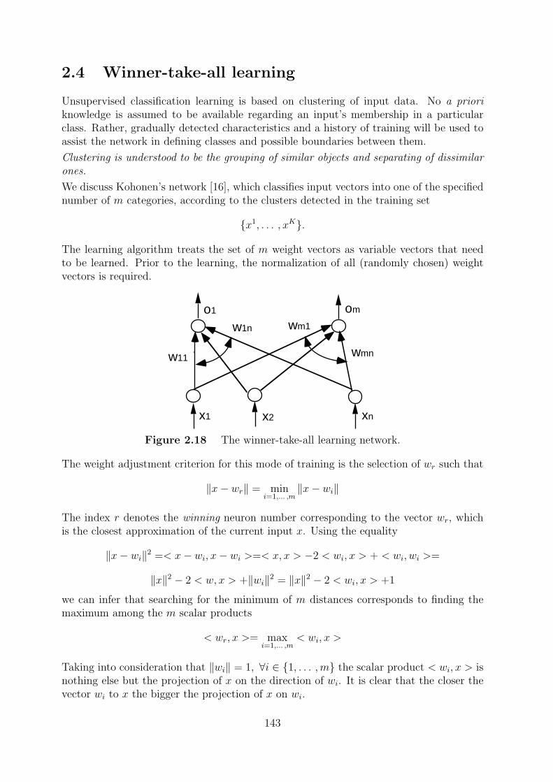
οm
x1 x2 xn
w11 wmn
ο1
w1n wm1
2.4 Winner-take-all learning
Unsupervised classification learning is based on clustering of input data. No a prioriknowledge is assumed to be available regarding an input’s membership in a particularclass. Rather, gradually detected characteristics and a history of training will be used toassist the network in defining classes and possible boundaries between them.
Clustering is understood to be the grouping of similar objects and separating of dissimilarones.
We discuss Kohonen’s network [16], which classifies input vectors into one of the specifiednumber of m categories, according to the clusters detected in the training set
{x1, . . . , xK}.
The learning algorithm treats the set of m weight vectors as variable vectors that needto be learned. Prior to the learning, the normalization of all (randomly chosen) weightvectors is required.
Figure 2.18 The winner-take-all learning network.
The weight adjustment criterion for this mode of training is the selection of wr such that
‖x− wr‖ = mini=1,... ,m
‖x− wi‖
The index r denotes the winning neuron number corresponding to the vector wr, whichis the closest approximation of the current input x. Using the equality
‖x− wi‖2 =< x− wi, x− wi >=< x, x > −2 < wi, x > + < wi, wi >=
‖x‖2 − 2 < w, x > +‖wi‖2 = ‖x‖2 − 2 < wi, x > +1
we can infer that searching for the minimum of m distances corresponds to finding themaximum among the m scalar products
< wr, x >= maxi=1,... ,m
< wi, x >
Taking into consideration that ‖wi‖ = 1, ∀i ∈ {1, . . . ,m} the scalar product < wi, x > isnothing else but the projection of x on the direction of wi. It is clear that the closer thevector wi to x the bigger the projection of x on wi.
143
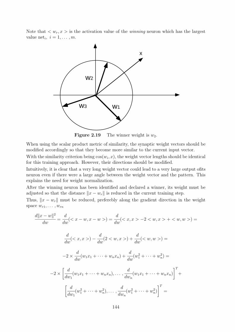
x
w1w3
w2
Note that < wr, x > is the activation value of the winning neuron which has the largestvalue neti, i = 1, . . . ,m.
Figure 2.19 The winner weight is w2.
When using the scalar product metric of similarity, the synaptic weight vectors should bemodified accordingly so that they become more similar to the current input vector.
With the similarity criterion being cos(wi, x), the weight vector lengths should be identicalfor this training approach. However, their directions should be modified.
Intuitively, it is clear that a very long weight vector could lead to a very large output ofitsneuron even if there were a large angle between the weight vector and the pattern. Thisexplains the need for weight normalization.
After the winning neuron has been identified and declared a winner, its weight must beadjusted so that the distance ‖x− wr‖ is reduced in the current training step.
Thus, ‖x − wr‖ must be reduced, preferebly along the gradient direction in the weightspace wr1, . . . , wrn
d‖x− w‖2
dw=
d
dw(< x− w, x− w >) =
d
dw(< x, x > −2 < w, x > + < w,w >) =
d
dw(< x, x >)−
d
dw(2 < w, x >) +
d
dw(< w,w >) =
−2×d
dw(w1x1 + · · ·+ wnxn) +
d
dw(w2
1 + · · ·+ w2n) =
−2×[d
dw1
(w1x1 + · · ·+ wnxn), . . . ,d
dwn(w1x1 + · · ·+ wnxn)
]T+
[d
dw1
(w21 + · · ·+ w2
n), . . . ,d
dwn(w2
1 + · · ·+ w2n)
]T=
144
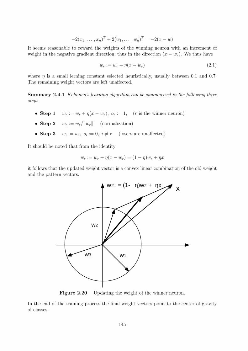
x
w1w3
w2
w2: = (1- η)w2 + ηx
−2(x1, . . . , xn)T + 2(w1, . . . , wn)T = −2(x− w)
It seems reasonable to reward the weights of the winning neuron with an increment ofweight in the negative gradient direction, thus in the direction (x− wr). We thus have
wr := wr + η(x− wr) (2.1)
where η is a small lerning constant selected heuristically, usually between 0.1 and 0.7.The remaining weight vectors are left unaffected.
Summary 2.4.1 Kohonen’s learning algorithm can be summarized in the following threesteps
• Step 1 wr := wr + η(x− wr), or := 1, (r is the winner neuron)
• Step 2 wr := wr/‖wr‖ (normalization)
• Step 3 wi := wi, oi := 0, i 6= r (losers are unaffected)
It should be noted that from the identity
wr := wr + η(x− wr) = (1− η)wr + ηx
it follows that the updated weight vector is a convex linear combination of the old weightand the pattern vectors.
Figure 2.20 Updating the weight of the winner neuron.
In the end of the training process the final weight vectors point to the center of gravityof classes.
145
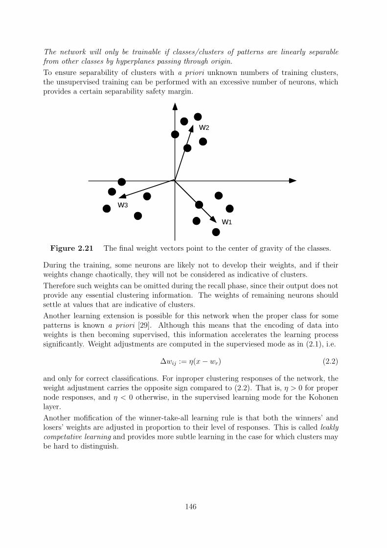
w1
w3
w2
The network will only be trainable if classes/clusters of patterns are linearly separablefrom other classes by hyperplanes passing through origin.
To ensure separability of clusters with a priori unknown numbers of training clusters,the unsupervised training can be performed with an excessive number of neurons, whichprovides a certain separability safety margin.
Figure 2.21 The final weight vectors point to the center of gravity of the classes.
During the training, some neurons are likely not to develop their weights, and if theirweights change chaotically, they will not be considered as indicative of clusters.
Therefore such weights can be omitted during the recall phase, since their output does notprovide any essential clustering information. The weights of remaining neurons shouldsettle at values that are indicative of clusters.
Another learning extension is possible for this network when the proper class for somepatterns is known a priori [29]. Although this means that the encoding of data intoweights is then becoming supervised, this information accelerates the learning processsignificantly. Weight adjustments are computed in the superviesed mode as in (2.1), i.e.
∆wij := η(x− wr) (2.2)
and only for correct classifications. For inproper clustering responses of the network, theweight adjustment carries the opposite sign compared to (2.2). That is, η > 0 for propernode responses, and η < 0 otherwise, in the supervised learning mode for the Kohonenlayer.
Another mofification of the winner-take-all learning rule is that both the winners’ andlosers’ weights are adjusted in proportion to their level of responses. This is called leaklycompetative learning and provides more subtle learning in the case for which clusters maybe hard to distinguish.
146
2.5 Applications of artificial neural networks
There are large classes of problems that appear to be more amenable to solution by neuralnetworks than by other available techniques. These tasks often involve ambiguity, such asthat inherent in handwritten character recognition. Problems of this sort are difficult totackle with conventional methods such as matched filtering or nearest neighbor classifica-tion, in part because the metrics used by the brain to compare patterns may not be veryclosely related to those chosen by an engineer designing a recognition system. Likewise,because reliable rules for recognizing a pattern are usually not at hand, fuzzy logic andexpert system designers also face the difficult and sometimes impossible task of findingacceptable descriptions of the complex relations governing class inclusion. In trainableneural network systems, these relations are abstracted directly from training data. More-over, because neural networks can be constructed with numbers of inputs and outputsranging into thousands, they can be used to attack problems that require consideration ofmore input variables than could be feasibly utilized by most other approaches. It shouldbe noted, however, that neural networks will not work well at solving problems for whichsufficiently large and general sets of training data are not obtainable. Drawing heavilyon [25] we provide a comprehensive list of applications of neural networks in Industry,Business and Science.
• The telecommunications industry. Many neural network applications are un-der development in the telecommunications industry for solving problems rangingfrom control of a nationwide switching network to management of an entire tele-phone company. Other aplications at the telephone circuit level turn out to bethe most significant commercial applications of neural networks in the world today.Modems, commonly used for computer-to-commputer communications and in ev-ery fax machine, have adaptive circuits for telephone line equalization and for echocancellation.
• Control of sound and vibration Active control of vibration and noise is accom-plished by using an adaptive actuator to generate equal and opposite vibration andnoise. This is being used in air-conditioning systems, in automotive systems, andin industrial applications.
• Particle accelerator beam control. The Stanford linear accelerator Center isnow using adaptive techniques to cancel disturbances that diminish the positioningaccuracy of opposing beams of positrons and electrons in a particle colloder.
• Credit card fraud detection. Several banks and credit card companies includingAmerican Express, Mellon Bank, First USA Bank, and others are currently usingneural networks to study patterns of credit card usage and and to detect transactionsthat are potentially fraudulent.
• Machine-printed character recognition. Commercial products performing ma-chine-printed character recognition have been introduced by a large number of com-panies and have been described in the literature.
• Hand-printed character recognition. Hecht-Nielsen Corp.’s Quickstrokes Au-tomated Data Entry System is being used to recognize handwritten forms at Avon’s
147
order-processing center and at the state of Wyoming’s Department of revenue. Inthe June 1992 issue of Systems Integration Business, Dennis Livingston reports thatbefore implementing the system, Wyoming was losing an estimated $300,000 peryear in interest income because so many cheks were being deposited late. CardiffSoftware offers a product called Teleform which uses Nestor’s hand-printed char-acter recognition system to convert a fax machine into an OCR scanner. PoqetComputer, now a subsidiary of Fujitsu, uses Nestor’s NestorWriter neural networksoftware to perform handwriting recognition for the penbased PC it announced inJanuary 1992 [26].
• Cursive handwriting recognition. Neural networks have proved useful in thedevelopment of algorithms for on-line cursive handwriting recognition [23]: A recentstartup company in Palo Alto, Lexicus, beginning with this basic technology hasdeveloped an impressive PC-based cursive handwriting system.
• Quality control in manufacturing. Neural networks are being used in a largenumber of quality control and quality assurance programs throughout industry.Applications include contaminant-level detection from spectroscopy data at chemicalplants and loudspeaker defect classification by CTS Electronics.
• Event detection in particle accelerators.
• Petroleum exploration. Oil companies including Arco and Texaco are usingneural networks to help determine the locations of underground oil and gas deposits.
• Medical applications. Commercial products by Neuromedical Systems Inc. areused for cancer screening and other medical applications [28]. The company marketselectrocardiograph and pap smear systems that rely on neural network technology.The pap smear system. Papnet, is able to help cytotechnologists spot cancerouscells, drastically reducing false/negative classifications. The system is used by theU.S. Food and Drug Administration [7].
• Financial forecasting and portfolio management. Neural networks are usedfor financial forecasting at a large number of investment firms and financial entitiesincluding Merill Lynch & Co., Salomon Brothers, Shearson Lehman Brothers Inc.,Citibank, and the World Bank. Using neural networks trained by genetic algorithms,Citibank’s Andrew Colin claims to be able to earn 25 % returns per year investingin the currency markets. A startup company, Promised Land Technologies, offers a$249 software package that is claimed to yield impressive annual returns [27].
• Loan approval. Chase Manhattan Bank reportedly uses a hybrid system utilizingpattern analysis and neural networks to evaluate corporate loan risk. Robert Marosereports in the May 1990 issue of AI Expert that the system, Creditview, helps loanofficers estimate the credit worthiness of corporate loan candidates.
• Real estate analysis
• Marketing analysis. The Target Marketing System developed by Churchill Sys-tem is currently in use by Veratex Corp. to optimize marketing strategy and cutmarketing costs by removing unlikely future customers from a list of potential cus-tomers [10].
148
• Electric arc furnace electrode position control. Electric arc furnaces are usedto melt scrap steel. The Intelligent Arc furnace controller systems installed byNeural Applications Corp. are reportedly saving millions of dollars per year perfurnace in increased furnace through-put and reduced electrode wear and electricityconsumption. The controller is currently being installed at furnaces worldwide.
• Semiconductor process control. Kopin Corp. has used neural networks to cutdopant concentration and deposition thickness errors in solar cell manufacturing bymore than a factor of two.
• Chemical process control. Pavilion Technologies has developed a neural networkprocess control package, Process Insights, which is helping Eastman Kodak and anumber of other companies reduce waste, improve product quality, and increaseplant throughput [9]. Neural network models are being used to perform sensitivitystudies, determine process set points, detect faults, and predict process performance.
• Petroleum refinery process control.
• Continuous-casting control during steel production
• Food and chemical formulation optimization.
• Nonlinear Applications on the Horizon. A large number of research programsare developing neural network solutions that are either likely to be used in the nearfuture or, particularly in the case of military applications, that may already beincorporated into products, albeit unadvertised. This category is much larger thanthe foregoing, so we present here only a few representative examples.
• Fighter flight and battle pattern quidance..
• Optical telescope focusing.
• Automobile applications. Ford Motor Co., General Motors, and other auto-mobile manufacturers are currently researching the possibility of widespread use ofneural networks in automobiles and in automobile production. Some of the areasthat are yielding promising results in the laboratory include engine fault detectionand diagnosis, antilock brake control, active-suspension control, and idle-speed con-trol. General Motors is having preliminary success using neural networks to modelsubjective customer ratings of automobiles based on their dynamic characteristicsto help engineers tailor vehicles to the market.
• Electric motor failure prediction. Siemens has reportedly developed a neu-ral network system that can accurately and inexpensively predict failure of largeinduction motors.
• Speech recognition. The Stanford Research Institute is currently involved inresearch combining neural networks with hidden Markov models and other tech-nologies in a highly successful speaker independent speech recognition system. Thetechnology will most likely be licensed to interested companies once perfected.
149
• Biomedical applications. Neural networks are rapidly finding diverse applica-tions in the biomedical sciences. They are being used widely in research on aminoacid sequencing in RNA and DNA, ECG and EEG waveform classification, pre-diction of patients’ reactions to drug treatments, prevention of anesthesia-relatedaccidents, arrhythmia recognition for implantable defibrillators patient mortalitypredictions, quantitative cytology, detection of breast cancer from mammograms,modeling schizophrenia, clinical diagnosis of lowerback pain, enhancement and clas-sification of medical images, lung nodule detection, diagnosis of hepatic masses,prediction of pulmonary embolism likelihood from ventilation-perfusion lung scans,and the study of interstitial lung disease.
• Drug development. One particularly promising area of medical research involvesthe use of neural networks in predicting the medicinal properties of substanceswithout expensive, time-consuming, and often inhumane animal testing.
• Control of copies. The Ricoh Corp. has successfully employed neural learningtechniques for control of several voltages in copies in order to preserve uniform copyquality despite changes in temperature, humidity, time since last copy, time sincechange in toner cartridge, and other variables. These variables influence copy qualityin highly nonlinear ways, which were learned through training of a backpropagationnetwork.
• The truck backer-upper. Vehicular control by artificial neural networks is atopic that has generated widespread interest. At Purdue University, tests havebeen performed using neural networks to control a model helicopter.
Perhaps the most important advantage of neural networks is their adaptivity. Neuralnetworks can automatically adjust their parameters (weights) to optimize their behavioras pattern recognizers, decision makers, system controllers, predictors, and so on.
Self-optimization allows the neural network to ”design” itself. The system designer firstdefines the neural network architecture, determines how the network connects to otherparts of the system, and chooses a training methodology for the network. The neuralnetwork then adapts to the application. Adaptivity allows the neural network to performwell even when the environment or the system being controlled varies over time. Thereare many control problems that can benefit from continual nonlinear modeling and adap-tation. Neural networks, such as those used by Pavilion in chemical process control, andby Neural Application Corp. in arc furnace control, are ideally suited to track problemsolutions in changing environments. Additionally, with some ”programmability”, such asthe choices regarding the number of neurons per layer and number of layers, a practitionercan use the same neural network in a wide variety of applications. Engineering time isthus saved.
Another example of the advantages of self-optimization is in the field of Expert Systems. Insome cases, instead of obtaining a set of rules through interaction between an experiencedexpert and a knowledge engineer, a neural system can be trained with examples of expertbehavior.
150
Bibliography
[1] I. Aleksander and H. Morton, An Introduction to Neural Computing (Chapmannand Hal, 1990).
[2] J.A. Anderson and E. Rosenfels eds., Neurocomputing: Foundations of Research(MIT Press, Cambridge, MA,1988).
[3] E. K. Blum and L. K. Li, Approximation theory and feedforward networks,Neural Networks, 4(1991) 511-515.
[4] P. Cardaliaguet, Approximation of a function and its derivative with a neuralnetwork, Neural Networks, 5(1992) 207-220.
[5] N.E.Cotter, The Stone-Weierstrass theorem and its applications to neural net-works, IEEE Transactions on Neural Networks, 1(1990) 290-295.
[6] J.E. Dayhoff, Neural Network Architectures: An Introduction (Van NostrandReinhold, New York,1990).
[7] A. Fuochi, Neural networks: No zealots yet but progress being made, Comput.Can., (January 20, 1992).
[8] K. Funahashi, On the Approximate Realization of Continuous Mappings by Neu-ral Networks, Neural Networks 2(1989) 183-192.
[9] C. Hall, Neural net technology: Ready for prime time? IEEE Expert (December1992) 2-4.
[10] D. Hammerstrom, Neural networks at work. IEEE Spectr. (June 1993) 26-32.
[11] D.O.Hebb, The Organization of Behavior (Wiley, New York, 1949).
[12] R.Hecht-Nielsen, Theory of the Backpropagation Neural Network, Proceedingsof International Conference on Neural Networks, Vol. 1, 1989 593-605.
[13] R.Hecht-Nielsen, Neurocomputing (Addison-Wesley Publishing Co., Reading,Mass., 1990).
[14] J.J.Hopfield, Neural networks and to physical systems with emergent collectivecomputational abilities, Proc. Natl. Acad. Sci., 79(1982) 2554-2558.
[15] K. Hornik, M. Stinchcombe and H. White, Universal Approximation of an Un-known Mapping and Its Derivatives Using Multilayer Freedforward Networks,Neural Networks, 3(1990) 551-560.
151
[16] T.Kohonen, Self-organization and Associative Memory, (Springer-Verlag, NewYork 1984).
[17] S.Y.Kung, Digital Neural Networks (Prentice Hall, Englewood Cliffs, New York,1993).
[18] V. Kurkova, Kolmogorov’s theorem and multilayer neural networks, Neural Net-works, 5(1992) 501-506.
[19] W.S.McCulloch and W.A.Pitts, A logical calculus of the ideas imminent in ner-vous activity, Bull. Math. Biophys. 5(1943) 115-133.
[20] M. Minsky and S. Papert, Perceptrons (MIT Press, Cambridge, Mass., 1969).
[21] F.Rosenblatt, The perceptron: A probabilistic model for information storage andorganization in the brain, Physic. Rev, 65(1958) 386-408.
[22] D.E.Rumelhart and J.L. McClelland and the PDP Research Group, ParallelDistributed Processing: Explorations in the Microstructure of Cognition (MITPress/Bradford Books, Cambridge, Mass., 1986).
[23] D.E. Rumelhart, Theory to practice: A case study - recognizing cursive hand-writing. In Proceedings of the Third NEC Research Symposium. SIAM, Philadel-phia, Pa., 1993.
[24] D.E.Rumelhart, B.Widrow and M.A.Lehr, The basic ideas in neural networks,Communications of ACM, 37(1994) 87-92.
[25] D.E.Rumelhart, B.Widrow and M.A.Lehr, Neural Networks: Applications inIndustry, Business and Science, Communications of ACM, 37(1994) 93-105.
[26] E.I. Schwartz and J.B. Treece, Smart programs go to work: How applied intelli-gence software makes decisions for the real world. Business Week (Mar. 2, 1992)97-105.
[27] E.I. Schwartz, Where neural networks are already at work: Putting AI to workin the markets, Business Week (Nov. 2, 1992) 136-137.
[28] J. Shandle, Neural networks are ready for prime time, Elect. Des., (February 18,1993), 51-58.
[29] P.I.Simpson, Artificial Neural Systems: Foundations, Paradigms, Applications,and Implementation (Pergamon Press, New York, 1990).
[30] P.D.Wasserman, Advanced Methods in Neural Computing, Van Nostrand Rein-hold, New York 1993.
[31] H. White, Connectionist Nonparametric Regression: Multilayer feedforward Net-works Can Learn Arbitrary Mappings, Neural Networks 3(1990) 535-549.
[32] J.M.Zurada, Introduction to Artificial Neural Systems (West Publishing Com-pany, New York, 1992).
152
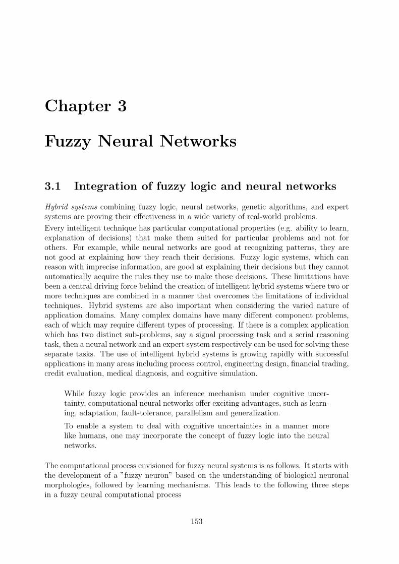
Chapter 3
Fuzzy Neural Networks
3.1 Integration of fuzzy logic and neural networks
Hybrid systems combining fuzzy logic, neural networks, genetic algorithms, and expertsystems are proving their effectiveness in a wide variety of real-world problems.
Every intelligent technique has particular computational properties (e.g. ability to learn,explanation of decisions) that make them suited for particular problems and not forothers. For example, while neural networks are good at recognizing patterns, they arenot good at explaining how they reach their decisions. Fuzzy logic systems, which canreason with imprecise information, are good at explaining their decisions but they cannotautomatically acquire the rules they use to make those decisions. These limitations havebeen a central driving force behind the creation of intelligent hybrid systems where two ormore techniques are combined in a manner that overcomes the limitations of individualtechniques. Hybrid systems are also important when considering the varied nature ofapplication domains. Many complex domains have many different component problems,each of which may require different types of processing. If there is a complex applicationwhich has two distinct sub-problems, say a signal processing task and a serial reasoningtask, then a neural network and an expert system respectively can be used for solving theseseparate tasks. The use of intelligent hybrid systems is growing rapidly with successfulapplications in many areas including process control, engineering design, financial trading,credit evaluation, medical diagnosis, and cognitive simulation.
While fuzzy logic provides an inference mechanism under cognitive uncer-tainty, computational neural networks offer exciting advantages, such as learn-ing, adaptation, fault-tolerance, parallelism and generalization.
To enable a system to deal with cognitive uncertainties in a manner morelike humans, one may incorporate the concept of fuzzy logic into the neuralnetworks.
The computational process envisioned for fuzzy neural systems is as follows. It starts withthe development of a ”fuzzy neuron” based on the understanding of biological neuronalmorphologies, followed by learning mechanisms. This leads to the following three stepsin a fuzzy neural computational process
153
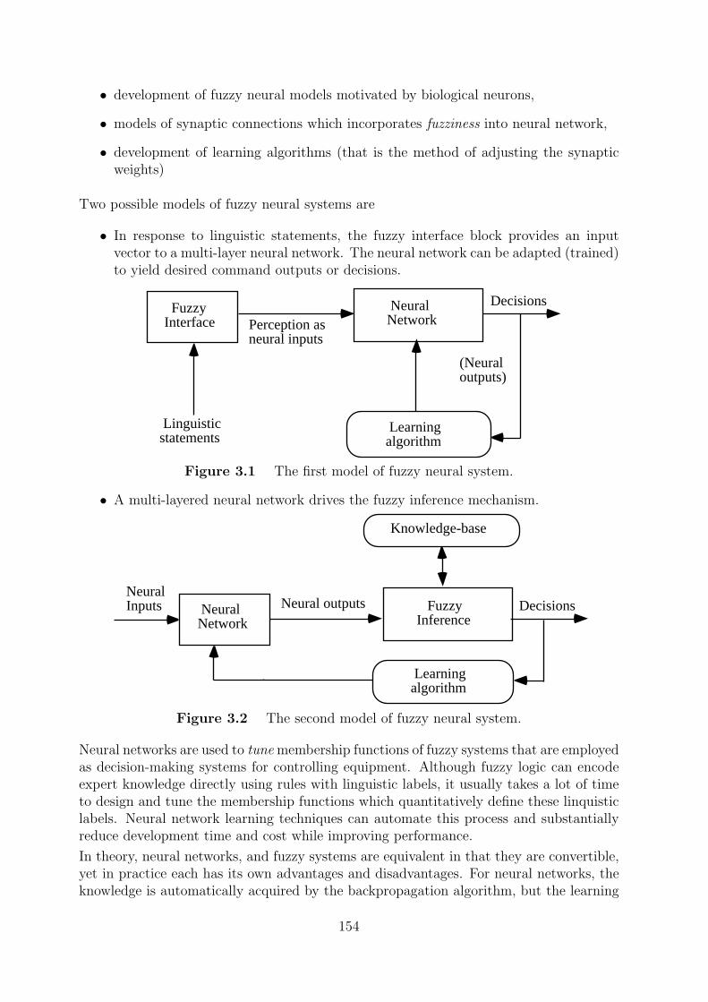
Linguisticstatements
NeuralNetwork
Decisions
Perception asneural inputs
(Neuraloutputs)
FuzzyInterface
Learningalgorithm
Neural Inputs Decisions Fuzzy
InferenceNeural outputs Neural
Network
Learningalgorithm
Knowledge-base
• development of fuzzy neural models motivated by biological neurons,
• models of synaptic connections which incorporates fuzziness into neural network,
• development of learning algorithms (that is the method of adjusting the synapticweights)
Two possible models of fuzzy neural systems are
• In response to linguistic statements, the fuzzy interface block provides an inputvector to a multi-layer neural network. The neural network can be adapted (trained)to yield desired command outputs or decisions.
Figure 3.1 The first model of fuzzy neural system.
• A multi-layered neural network drives the fuzzy inference mechanism.
Figure 3.2 The second model of fuzzy neural system.
Neural networks are used to tune membership functions of fuzzy systems that are employedas decision-making systems for controlling equipment. Although fuzzy logic can encodeexpert knowledge directly using rules with linguistic labels, it usually takes a lot of timeto design and tune the membership functions which quantitatively define these linquisticlabels. Neural network learning techniques can automate this process and substantiallyreduce development time and cost while improving performance.
In theory, neural networks, and fuzzy systems are equivalent in that they are convertible,yet in practice each has its own advantages and disadvantages. For neural networks, theknowledge is automatically acquired by the backpropagation algorithm, but the learning
154
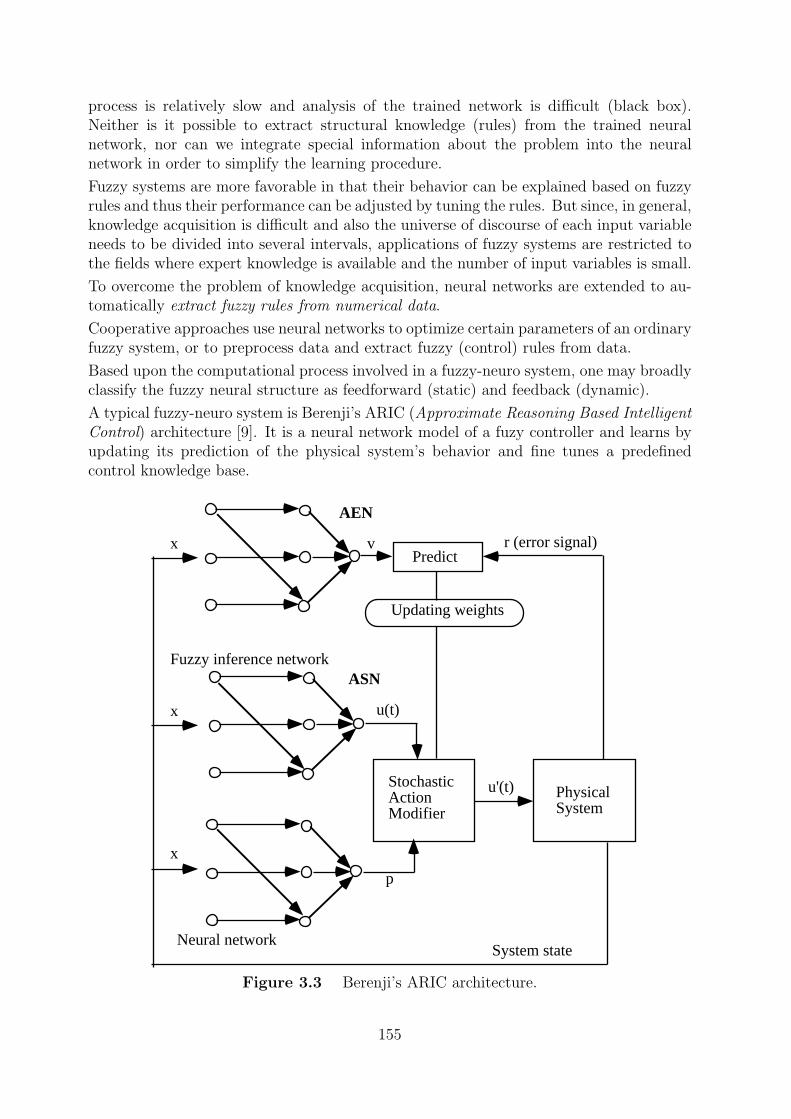
Predict
StochasticActionModifier
PhysicalSystem
AEN
ASN
u(t)
p
Fuzzy inference network
x
x
x
v
u'(t)
System stateNeural network
r (error signal)
Updating weights
process is relatively slow and analysis of the trained network is difficult (black box).Neither is it possible to extract structural knowledge (rules) from the trained neuralnetwork, nor can we integrate special information about the problem into the neuralnetwork in order to simplify the learning procedure.
Fuzzy systems are more favorable in that their behavior can be explained based on fuzzyrules and thus their performance can be adjusted by tuning the rules. But since, in general,knowledge acquisition is difficult and also the universe of discourse of each input variableneeds to be divided into several intervals, applications of fuzzy systems are restricted tothe fields where expert knowledge is available and the number of input variables is small.
To overcome the problem of knowledge acquisition, neural networks are extended to au-tomatically extract fuzzy rules from numerical data.
Cooperative approaches use neural networks to optimize certain parameters of an ordinaryfuzzy system, or to preprocess data and extract fuzzy (control) rules from data.
Based upon the computational process involved in a fuzzy-neuro system, one may broadlyclassify the fuzzy neural structure as feedforward (static) and feedback (dynamic).
A typical fuzzy-neuro system is Berenji’s ARIC (Approximate Reasoning Based IntelligentControl) architecture [9]. It is a neural network model of a fuzy controller and learns byupdating its prediction of the physical system’s behavior and fine tunes a predefinedcontrol knowledge base.
Figure 3.3 Berenji’s ARIC architecture.
155
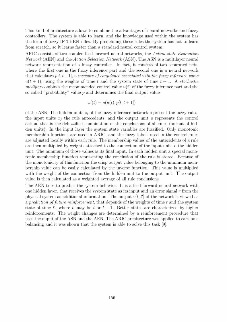
This kind of architecture allows to combine the advantages of neural networks and fuzzycontrollers. The system is able to learn, and the knowledge used within the system hasthe form of fuzzy IF-THEN rules. By predefining these rules the system has not to learnfrom scratch, so it learns faster than a standard neural control system.
ARIC consists of two coupled feed-forward neural networks, the Action-state EvaluationNetwork (AEN) and the Action Selection Network (ASN). The ASN is a multilayer neuralnetwork representation of a fuzzy controller. In fact, it consists of two separated nets,where the first one is the fuzzy inference part and the second one is a neural networkthat calculates p[t, t+1], a measure of confidence associated with the fuzzy inference valueu(t + 1), using the weights of time t and the system state of time t + 1. A stochasticmodifier combines the recommended control value u(t) of the fuzzy inference part and theso called ”probability” value p and determines the final output value
u′(t) = o(u(t), p[t, t+ 1])
of the ASN. The hidden units zi of the fuzzy inference network represent the fuzzy rules,the input units xj the rule antecedents, and the output unit u represents the controlaction, that is the defuzzified combination of the conclusions of all rules (output of hid-den units). In the input layer the system state variables are fuzzified. Only monotonicmembership functions are used in ARIC, and the fuzzy labels used in the control rulesare adjusted locally within each rule. The membership values of the antecedents of a ruleare then multiplied by weights attached to the connection of the input unit to the hiddenunit. The minimum of those values is its final input. In each hidden unit a special mono-tonic membership function representing the conclusion of the rule is stored. Because ofthe monotonicity of this function the crisp output value belonging to the minimum mem-bership value can be easily calculated by the inverse function. This value is multipliedwith the weight of the connection from the hidden unit to the output unit. The outputvalue is then calculated as a weighted average of all rule conclusions.
The AEN tries to predict the system behavior. It is a feed-forward neural network withone hidden layer, that receives the system state as its input and an error signal r from thephysical system as additional information. The output v[t, t′] of the network is viewed asa prediction of future reinforcement, that depends of the weights of time t and the systemstate of time t′, where t′ may be t or t + 1. Better states are characterized by higherreinforcements. The weight changes are determined by a reinforcement procedure thatuses the ouput of the ASN and the AEN. The ARIC architecture was applied to cart-polebalancing and it was shown that the system is able to solve this task [9].
156
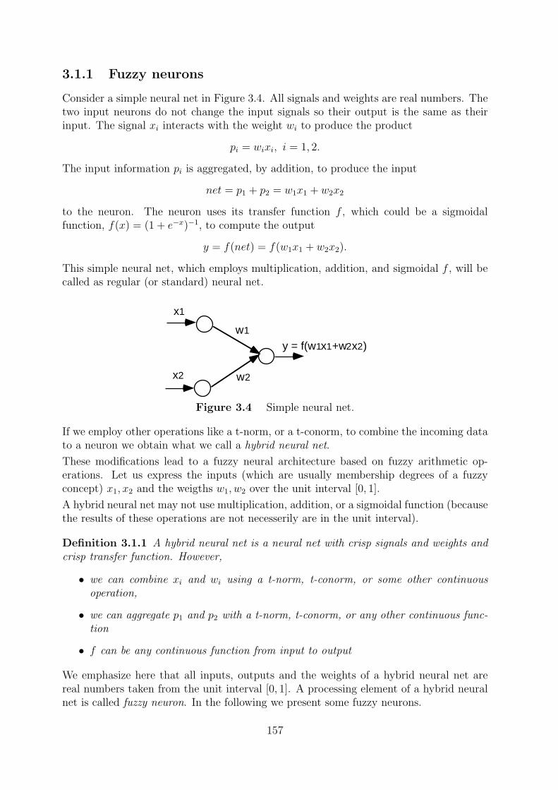
x1
x2
w1
w2
y = f(w1x1+w2x2)
3.1.1 Fuzzy neurons
Consider a simple neural net in Figure 3.4. All signals and weights are real numbers. Thetwo input neurons do not change the input signals so their output is the same as theirinput. The signal xi interacts with the weight wi to produce the product
pi = wixi, i = 1, 2.
The input information pi is aggregated, by addition, to produce the input
net = p1 + p2 = w1x1 + w2x2
to the neuron. The neuron uses its transfer function f , which could be a sigmoidalfunction, f(x) = (1 + e−x)−1, to compute the output
y = f(net) = f(w1x1 + w2x2).
This simple neural net, which employs multiplication, addition, and sigmoidal f , will becalled as regular (or standard) neural net.
Figure 3.4 Simple neural net.
If we employ other operations like a t-norm, or a t-conorm, to combine the incoming datato a neuron we obtain what we call a hybrid neural net.
These modifications lead to a fuzzy neural architecture based on fuzzy arithmetic op-erations. Let us express the inputs (which are usually membership degrees of a fuzzyconcept) x1, x2 and the weigths w1, w2 over the unit interval [0, 1].
A hybrid neural net may not use multiplication, addition, or a sigmoidal function (becausethe results of these operations are not necesserily are in the unit interval).
Definition 3.1.1 A hybrid neural net is a neural net with crisp signals and weights andcrisp transfer function. However,
• we can combine xi and wi using a t-norm, t-conorm, or some other continuousoperation,
• we can aggregate p1 and p2 with a t-norm, t-conorm, or any other continuous func-tion
• f can be any continuous function from input to output
We emphasize here that all inputs, outputs and the weights of a hybrid neural net arereal numbers taken from the unit interval [0, 1]. A processing element of a hybrid neuralnet is called fuzzy neuron. In the following we present some fuzzy neurons.
157
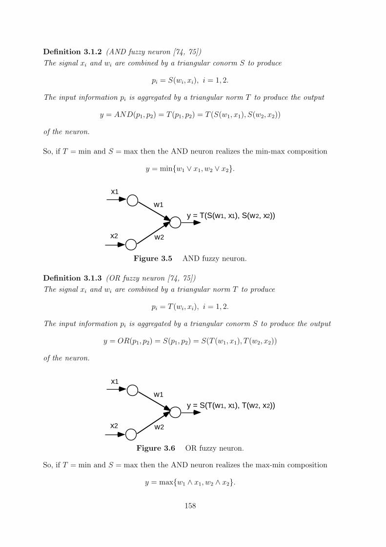
x1
x2
w1
w2
y = T(S(w1, x1), S(w2, x2))
x1
x2
w1
w2
y = S(T(w1, x1), T(w2, x2))
Definition 3.1.2 (AND fuzzy neuron [74, 75])
The signal xi and wi are combined by a triangular conorm S to produce
pi = S(wi, xi), i = 1, 2.
The input information pi is aggregated by a triangular norm T to produce the output
y = AND(p1, p2) = T (p1, p2) = T (S(w1, x1), S(w2, x2))
of the neuron.
So, if T = min and S = max then the AND neuron realizes the min-max composition
y = min{w1 ∨ x1, w2 ∨ x2}.
Figure 3.5 AND fuzzy neuron.
Definition 3.1.3 (OR fuzzy neuron [74, 75])
The signal xi and wi are combined by a triangular norm T to produce
pi = T (wi, xi), i = 1, 2.
The input information pi is aggregated by a triangular conorm S to produce the output
y = OR(p1, p2) = S(p1, p2) = S(T (w1, x1), T (w2, x2))
of the neuron.
Figure 3.6 OR fuzzy neuron.
So, if T = min and S = max then the AND neuron realizes the max-min composition
y = max{w1 ∧ x1, w2 ∧ x2}.
158
x1
x2
w1
w2
y=S(w1←x1, w2 ← x2)
The AND and OR fuzzy neurons realize pure logic operations on the membership values.The role of the connections is to differentiate between particular leveles of impact thatthe individual inputs might have on the result of aggregation. We note that (i) the higherthe value wi the stronger the impact of xi on the output y of an OR neuron, (ii) the lowerthe value wi the stronger the impact of xi on the output y of an AND neuron.
The range of the output value y for the AND neuron is computed by letting all xi equalto zero or one. In virtue of the monotonicity property of triangular norms, we obtain
y ∈ [T (w1, w2), 1]
and for the OR neuron one derives the boundaries
y ∈ [0, S(w1, w2)].
Definition 3.1.4 (Implication-OR fuzzy neuron [37, 39])
The signal xi and wi are combined by a fuzzy implication operator I to produce
pi = I(wi, xi) = wi ← xi, i = 1, 2.
The input information pi is aggregated by a triangular conorm S to produce the output
y = I(p1, p2) = S(p1, p2) = S(w1 ← x1, w2 ← x2)
of the neuron.
Figure 3.7 Implication-OR fuzzy neuron.
Definition 3.1.5 (Kwan and Cai’s fuzzy neuron [111])
The signal xi interacts with the weight wi to produce the product
pi = wixi, i = 1, . . . , n
The input information pi is aggregated by an agregation function h to produce the inputof the neuron
z = h(w1x1, w2x2, . . . , wnxn)
the state of the neuron is computed by
s = f(z − θ)where f is an activation function and θ is the activating threshold. And the m outputs ofthe neuron are computed by
yj = gj(s), j = 1, . . . ,m
where gj, j = 1, . . . ,m are the m output functions of the neuron which represent themembership functions of the input pattern x1, x2, . . . , xn in all the m fuzzy sets.
159
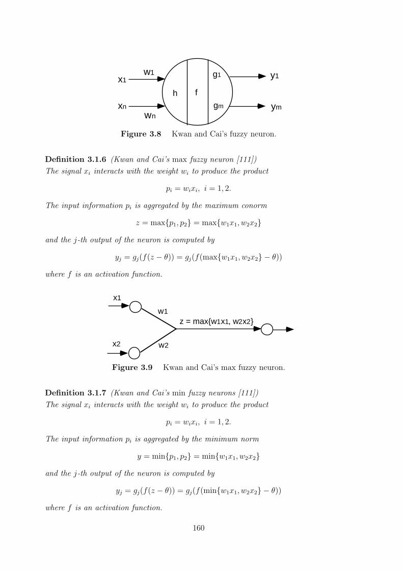
h f
g1
gm
x1
xn
w1
wn
y1
ym
x1
x2
w1
w2
z = max{w1x1, w2x2}
Figure 3.8 Kwan and Cai’s fuzzy neuron.
Definition 3.1.6 (Kwan and Cai’s max fuzzy neuron [111])
The signal xi interacts with the weight wi to produce the product
pi = wixi, i = 1, 2.
The input information pi is aggregated by the maximum conorm
z = max{p1, p2} = max{w1x1, w2x2}
and the j-th output of the neuron is computed by
yj = gj(f(z − θ)) = gj(f(max{w1x1, w2x2} − θ))
where f is an activation function.
Figure 3.9 Kwan and Cai’s max fuzzy neuron.
Definition 3.1.7 (Kwan and Cai’s min fuzzy neurons [111])
The signal xi interacts with the weight wi to produce the product
pi = wixi, i = 1, 2.
The input information pi is aggregated by the minimum norm
y = min{p1, p2} = min{w1x1, w2x2}
and the j-th output of the neuron is computed by
yj = gj(f(z − θ)) = gj(f(min{w1x1, w2x2} − θ))
where f is an activation function.
160
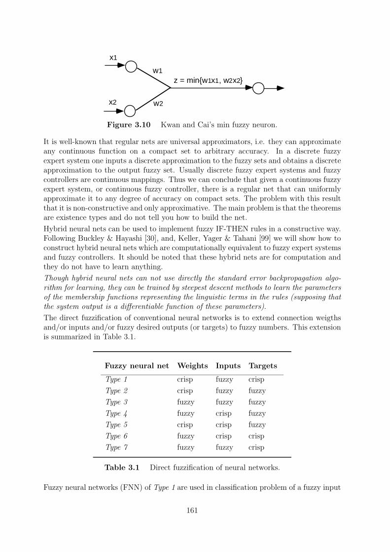
x1
x2
w1
w2
z = min{w1x1, w2x2}
Figure 3.10 Kwan and Cai’s min fuzzy neuron.
It is well-known that regular nets are universal approximators, i.e. they can approximateany continuous function on a compact set to arbitrary accuracy. In a discrete fuzzyexpert system one inputs a discrete approximation to the fuzzy sets and obtains a discreteapproximation to the output fuzzy set. Usually discrete fuzzy expert systems and fuzzycontrollers are continuous mappings. Thus we can conclude that given a continuous fuzzyexpert system, or continuous fuzzy controller, there is a regular net that can uniformlyapproximate it to any degree of accuracy on compact sets. The problem with this resultthat it is non-constructive and only approximative. The main problem is that the theoremsare existence types and do not tell you how to build the net.
Hybrid neural nets can be used to implement fuzzy IF-THEN rules in a constructive way.Following Buckley & Hayashi [30], and, Keller, Yager & Tahani [99] we will show how toconstruct hybrid neural nets which are computationally equivalent to fuzzy expert systemsand fuzzy controllers. It should be noted that these hybrid nets are for computation andthey do not have to learn anything.
Though hybrid neural nets can not use directly the standard error backpropagation algo-rithm for learning, they can be trained by steepest descent methods to learn the parametersof the membership functions representing the linguistic terms in the rules (supposing thatthe system output is a differentiable function of these parameters).
The direct fuzzification of conventional neural networks is to extend connection weigthsand/or inputs and/or fuzzy desired outputs (or targets) to fuzzy numbers. This extensionis summarized in Table 3.1.
Fuzzy neural net Weights Inputs Targets
Type 1 crisp fuzzy crisp
Type 2 crisp fuzzy fuzzy
Type 3 fuzzy fuzzy fuzzy
Type 4 fuzzy crisp fuzzy
Type 5 crisp crisp fuzzy
Type 6 fuzzy crisp crisp
Type 7 fuzzy fuzzy crisp
Table 3.1 Direct fuzzification of neural networks.
Fuzzy neural networks (FNN) of Type 1 are used in classification problem of a fuzzy input
161
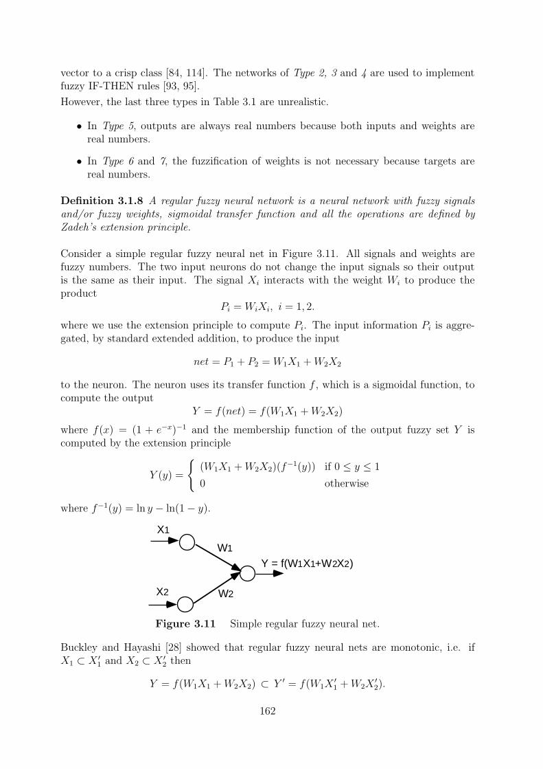
X1
X2
W1
W2
Y = f(W1X1+W2X2)
vector to a crisp class [84, 114]. The networks of Type 2, 3 and 4 are used to implementfuzzy IF-THEN rules [93, 95].
However, the last three types in Table 3.1 are unrealistic.
• In Type 5, outputs are always real numbers because both inputs and weights arereal numbers.
• In Type 6 and 7, the fuzzification of weights is not necessary because targets arereal numbers.
Definition 3.1.8 A regular fuzzy neural network is a neural network with fuzzy signalsand/or fuzzy weights, sigmoidal transfer function and all the operations are defined byZadeh’s extension principle.
Consider a simple regular fuzzy neural net in Figure 3.11. All signals and weights arefuzzy numbers. The two input neurons do not change the input signals so their outputis the same as their input. The signal Xi interacts with the weight Wi to produce theproduct
Pi = WiXi, i = 1, 2.
where we use the extension principle to compute Pi. The input information Pi is aggre-gated, by standard extended addition, to produce the input
net = P1 + P2 = W1X1 +W2X2
to the neuron. The neuron uses its transfer function f , which is a sigmoidal function, tocompute the output
Y = f(net) = f(W1X1 +W2X2)
where f(x) = (1 + e−x)−1 and the membership function of the output fuzzy set Y iscomputed by the extension principle
Y (y) =
{(W1X1 +W2X2)(f−1(y)) if 0 ≤ y ≤ 1
0 otherwise
where f−1(y) = ln y − ln(1− y).
Figure 3.11 Simple regular fuzzy neural net.
Buckley and Hayashi [28] showed that regular fuzzy neural nets are monotonic, i.e. ifX1 ⊂ X ′1 and X2 ⊂ X ′2 then
Y = f(W1X1 +W2X2) ⊂ Y ′ = f(W1X′1 +W2X
′2).
162
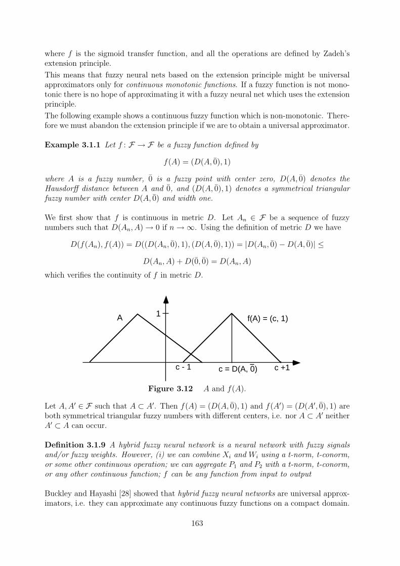
1A
c = D(A, 0)c - 1
f(A) = (c, 1)
c +1
where f is the sigmoid transfer function, and all the operations are defined by Zadeh’sextension principle.
This means that fuzzy neural nets based on the extension principle might be universalapproximators only for continuous monotonic functions. If a fuzzy function is not mono-tonic there is no hope of approximating it with a fuzzy neural net which uses the extensionprinciple.
The following example shows a continuous fuzzy function which is non-monotonic. There-fore we must abandon the extension principle if we are to obtain a universal approximator.
Example 3.1.1 Let f : F → F be a fuzzy function defined by
f(A) = (D(A, 0), 1)
where A is a fuzzy number, 0 is a fuzzy point with center zero, D(A, 0) denotes theHausdorff distance between A and 0, and (D(A, 0), 1) denotes a symmetrical triangularfuzzy number with center D(A, 0) and width one.
We first show that f is continuous in metric D. Let An ∈ F be a sequence of fuzzynumbers such that D(An, A)→ 0 if n→∞. Using the definition of metric D we have
D(f(An), f(A)) = D((D(An, 0), 1), (D(A, 0), 1)) = |D(An, 0)−D(A, 0)| ≤
D(An, A) +D(0, 0) = D(An, A)
which verifies the continuity of f in metric D.
Figure 3.12 A and f(A).
Let A,A′ ∈ F such that A ⊂ A′. Then f(A) = (D(A, 0), 1) and f(A′) = (D(A′, 0), 1) areboth symmetrical triangular fuzzy numbers with different centers, i.e. nor A ⊂ A′ neitherA′ ⊂ A can occur.
Definition 3.1.9 A hybrid fuzzy neural network is a neural network with fuzzy signalsand/or fuzzy weights. However, (i) we can combine Xi and Wi using a t-norm, t-conorm,or some other continuous operation; we can aggregate P1 and P2 with a t-norm, t-conorm,or any other continuous function; f can be any function from input to output
Buckley and Hayashi [28] showed that hybrid fuzzy neural networks are universal approx-imators, i.e. they can approximate any continuous fuzzy functions on a compact domain.
163
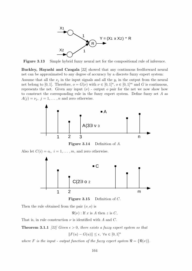
X1
X2 1
1
RY = (X1 x X2) ∗ R
1 2 n3
Α(3) = ν3
A
1 2
C
C(2) = ο2
m
Figure 3.13 Simple hybrid fuzzy neural net for the compositional rule of inference.
Buckley, Hayashi and Czogala [22] showed that any continuous feedforward neuralnet can be approximated to any degree of accuracy by a discrete fuzzy expert system:
Assume that all the νj in the input signals and all the yi in the output from the neuralnet belong to [0, 1]. Therefore, o = G(ν) with ν ∈ [0, 1]n, o ∈ [0, 1]m and G is continuous,represents the net. Given any input (ν) - output o pair for the net we now show howto construct the corresponding rule in the fuzzy expert system. Define fuzzy set A asA(j) = νj, j = 1, . . . , n and zero otherwise.
Figure 3.14 Definition of A.
Also let C(i) = oi, i = 1, . . . ,m, and zero otherwise.
Figure 3.15 Definition of C.
Then the rule obtained from the pair (ν, o) is
<(ν) : If x is A then z is C,
That is, in rule construction ν is identified with A and C.
Theorem 3.1.1 [22] Given ε > 0, there exists a fuzzy expert system so that
‖F (u)−G(u)‖ ≤ ε, ∀u ∈ [0, 1]n
where F is the input - output function of the fuzzy expert system < = {<(ν)}.
164
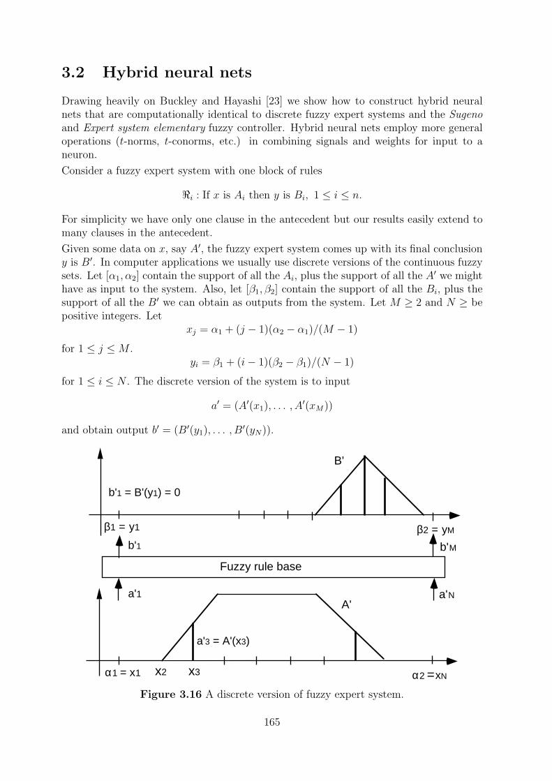
x2
β2 = yM
x3 α2 =xN α1 = x1
β1 = y1
A'
B'
a'3 = A'(x3)
Fuzzy rule base
a'1 a'N
b'1 b'M
b'1 = B'(y1) = 0
3.2 Hybrid neural nets
Drawing heavily on Buckley and Hayashi [23] we show how to construct hybrid neuralnets that are computationally identical to discrete fuzzy expert systems and the Sugenoand Expert system elementary fuzzy controller. Hybrid neural nets employ more generaloperations (t-norms, t-conorms, etc.) in combining signals and weights for input to aneuron.
Consider a fuzzy expert system with one block of rules
<i : If x is Ai then y is Bi, 1 ≤ i ≤ n.
For simplicity we have only one clause in the antecedent but our results easily extend tomany clauses in the antecedent.
Given some data on x, say A′, the fuzzy expert system comes up with its final conclusiony is B′. In computer applications we usually use discrete versions of the continuous fuzzysets. Let [α1, α2] contain the support of all the Ai, plus the support of all the A′ we mighthave as input to the system. Also, let [β1, β2] contain the support of all the Bi, plus thesupport of all the B′ we can obtain as outputs from the system. Let M ≥ 2 and N ≥ bepositive integers. Let
xj = α1 + (j − 1)(α2 − α1)/(M − 1)
for 1 ≤ j ≤M .yi = β1 + (i− 1)(β2 − β1)/(N − 1)
for 1 ≤ i ≤ N . The discrete version of the system is to input
a′ = (A′(x1), . . . , A′(xM))
and obtain output b′ = (B′(y1), . . . , B′(yN)).
Figure 3.16 A discrete version of fuzzy expert system.
165
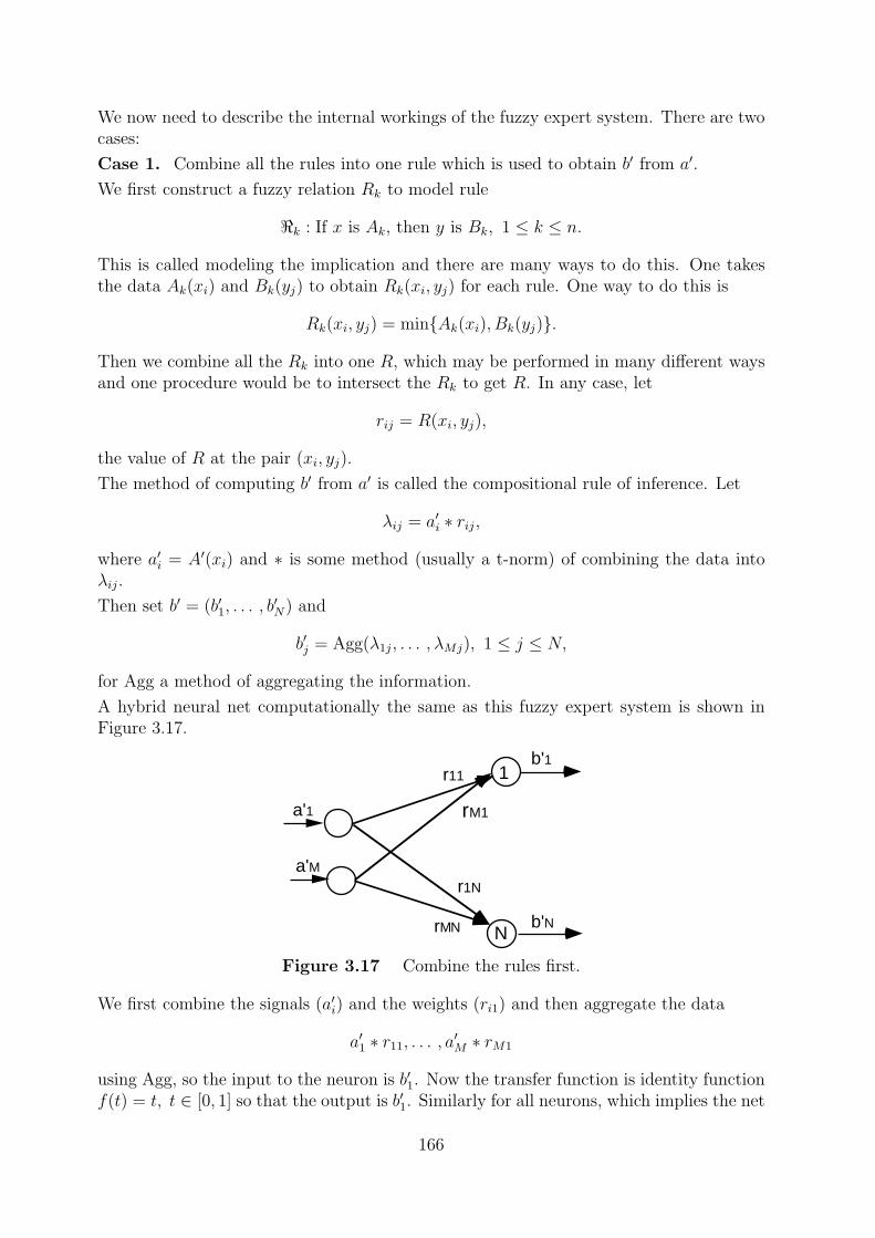
a'1
a'M
b'1
b'N
r11
rM1
r1N
rMN
1
N
We now need to describe the internal workings of the fuzzy expert system. There are twocases:
Case 1. Combine all the rules into one rule which is used to obtain b′ from a′.
We first construct a fuzzy relation Rk to model rule
<k : If x is Ak, then y is Bk, 1 ≤ k ≤ n.
This is called modeling the implication and there are many ways to do this. One takesthe data Ak(xi) and Bk(yj) to obtain Rk(xi, yj) for each rule. One way to do this is
Rk(xi, yj) = min{Ak(xi), Bk(yj)}.
Then we combine all the Rk into one R, which may be performed in many different waysand one procedure would be to intersect the Rk to get R. In any case, let
rij = R(xi, yj),
the value of R at the pair (xi, yj).
The method of computing b′ from a′ is called the compositional rule of inference. Let
λij = a′i ∗ rij,
where a′i = A′(xi) and ∗ is some method (usually a t-norm) of combining the data intoλij.
Then set b′ = (b′1, . . . , b′N) and
b′j = Agg(λ1j, . . . , λMj), 1 ≤ j ≤ N,
for Agg a method of aggregating the information.
A hybrid neural net computationally the same as this fuzzy expert system is shown inFigure 3.17.
Figure 3.17 Combine the rules first.
We first combine the signals (a′i) and the weights (ri1) and then aggregate the data
a′1 ∗ r11, . . . , a′M ∗ rM1
using Agg, so the input to the neuron is b′1. Now the transfer function is identity functionf(t) = t, t ∈ [0, 1] so that the output is b′1. Similarly for all neurons, which implies the net
166
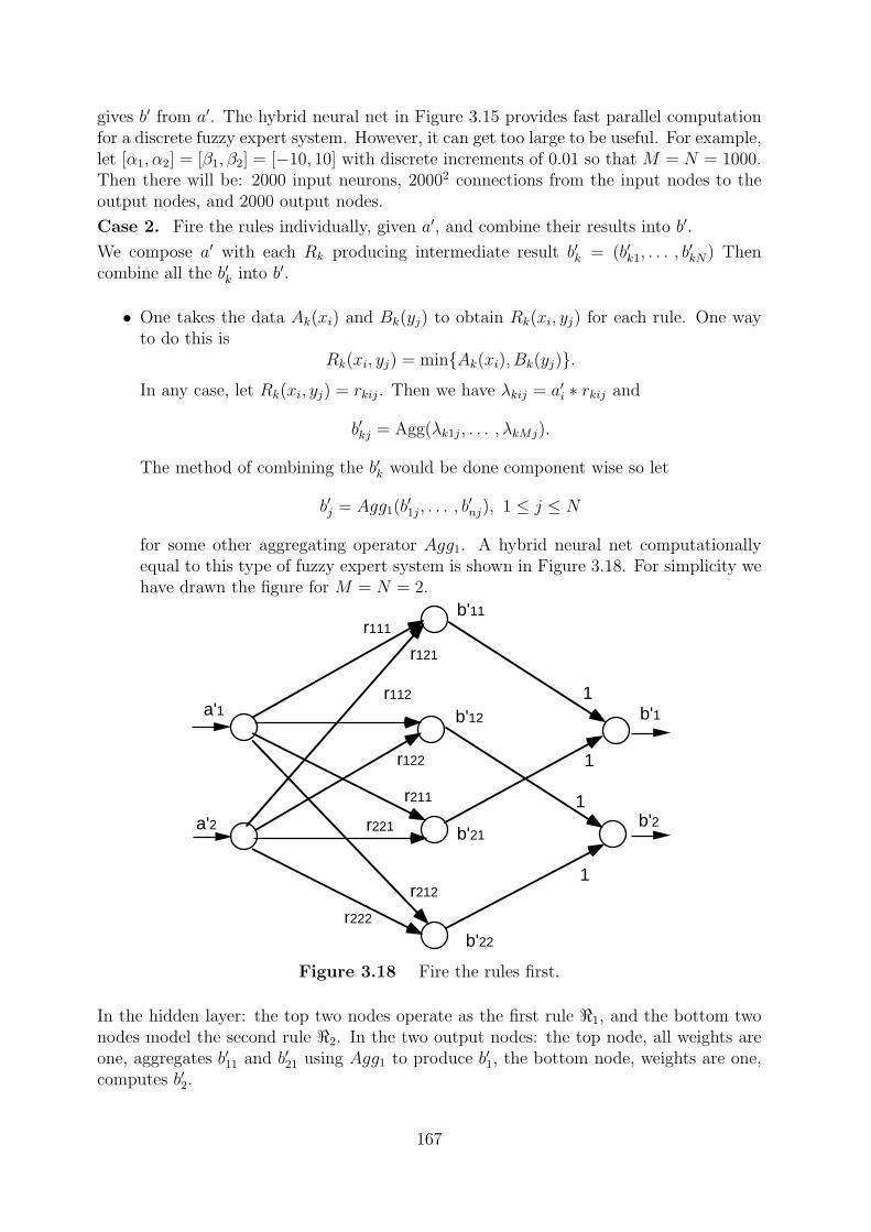
a'1
a'2
b'1
b'2
1
1
1
1
r111
r121
r112
r122
r211
r221
r212
r222
b'11
b'12
b'21
b'22
gives b′ from a′. The hybrid neural net in Figure 3.15 provides fast parallel computationfor a discrete fuzzy expert system. However, it can get too large to be useful. For example,let [α1, α2] = [β1, β2] = [−10, 10] with discrete increments of 0.01 so that M = N = 1000.Then there will be: 2000 input neurons, 20002 connections from the input nodes to theoutput nodes, and 2000 output nodes.
Case 2. Fire the rules individually, given a′, and combine their results into b′.
We compose a′ with each Rk producing intermediate result b′k = (b′k1, . . . , b′kN) Then
combine all the b′k into b′.
• One takes the data Ak(xi) and Bk(yj) to obtain Rk(xi, yj) for each rule. One wayto do this is
Rk(xi, yj) = min{Ak(xi), Bk(yj)}.In any case, let Rk(xi, yj) = rkij. Then we have λkij = a′i ∗ rkij and
b′kj = Agg(λk1j, . . . , λkMj).
The method of combining the b′k would be done component wise so let
b′j = Agg1(b′1j, . . . , b′nj), 1 ≤ j ≤ N
for some other aggregating operator Agg1. A hybrid neural net computationallyequal to this type of fuzzy expert system is shown in Figure 3.18. For simplicity wehave drawn the figure for M = N = 2.
Figure 3.18 Fire the rules first.
In the hidden layer: the top two nodes operate as the first rule <1, and the bottom twonodes model the second rule <2. In the two output nodes: the top node, all weights areone, aggregates b′11 and b′21 using Agg1 to produce b′1, the bottom node, weights are one,computes b′2.
167
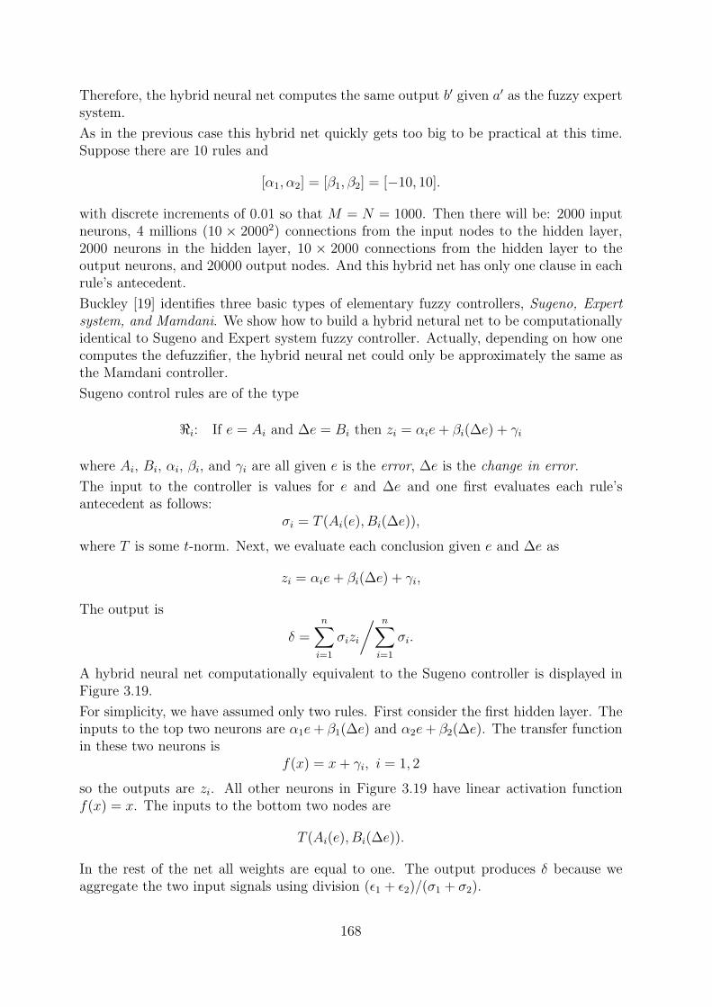
Therefore, the hybrid neural net computes the same output b′ given a′ as the fuzzy expertsystem.
As in the previous case this hybrid net quickly gets too big to be practical at this time.Suppose there are 10 rules and
[α1, α2] = [β1, β2] = [−10, 10].
with discrete increments of 0.01 so that M = N = 1000. Then there will be: 2000 inputneurons, 4 millions (10 × 20002) connections from the input nodes to the hidden layer,2000 neurons in the hidden layer, 10 × 2000 connections from the hidden layer to theoutput neurons, and 20000 output nodes. And this hybrid net has only one clause in eachrule’s antecedent.
Buckley [19] identifies three basic types of elementary fuzzy controllers, Sugeno, Expertsystem, and Mamdani. We show how to build a hybrid netural net to be computationallyidentical to Sugeno and Expert system fuzzy controller. Actually, depending on how onecomputes the defuzzifier, the hybrid neural net could only be approximately the same asthe Mamdani controller.
Sugeno control rules are of the type
<i: If e = Ai and ∆e = Bi then zi = αie+ βi(∆e) + γi
where Ai, Bi, αi, βi, and γi are all given e is the error, ∆e is the change in error.
The input to the controller is values for e and ∆e and one first evaluates each rule’santecedent as follows:
σi = T (Ai(e), Bi(∆e)),
where T is some t-norm. Next, we evaluate each conclusion given e and ∆e as
zi = αie+ βi(∆e) + γi,
The output is
δ =n∑i=1
σizi
/ n∑i=1
σi.
A hybrid neural net computationally equivalent to the Sugeno controller is displayed inFigure 3.19.
For simplicity, we have assumed only two rules. First consider the first hidden layer. Theinputs to the top two neurons are α1e+ β1(∆e) and α2e+ β2(∆e). The transfer functionin these two neurons is
f(x) = x+ γi, i = 1, 2
so the outputs are zi. All other neurons in Figure 3.19 have linear activation functionf(x) = x. The inputs to the bottom two nodes are
T (Ai(e), Bi(∆e)).
In the rest of the net all weights are equal to one. The output produces δ because weaggregate the two input signals using division (ε1 + ε2)/(σ1 + σ2).
168
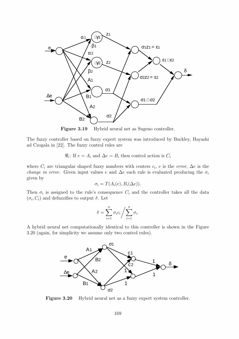
e
δ
α1
α2
β1
β2
z2
z1+γ1
+γ2
B1
B2
A2
A1
σ1
σ2
∆eσ1 + σ2
ε1 + ε2
σ1z1 = ε1
σ2z2 = ε2
e
∆e
δ1
1
A1
B1
A2
B2
σ1
σ2
c1
c2
1
1
Figure 3.19 Hybrid neural net as Sugeno controller.
The fuzzy controller based on fuzzy expert system was introduced by Buckley, Hayashiad Czogala in [22]. The fuzzy control rules are
<i: If e = Ai and ∆e = Bi then control action is Ci
where Ci are triangular shaped fuzzy numbers with centers ci, e is the error, ∆e is thechange in error. Given input values e and ∆e each rule is evaluated producing the σigiven by
σi = T (Ai(e), Bi(∆e)).
Then σi is assigned to the rule’s consequence Ci and the controller takes all the data(σi, Ci) and defuzzifies to output δ. Let
δ =n∑i=1
σici
/ n∑i=1
σi.
A hybrid neural net computationally identical to this controller is shown in the Figure3.20 (again, for simplicity we assume only two control rules).
Figure 3.20 Hybrid neural net as a fuzzy expert system controller.
169
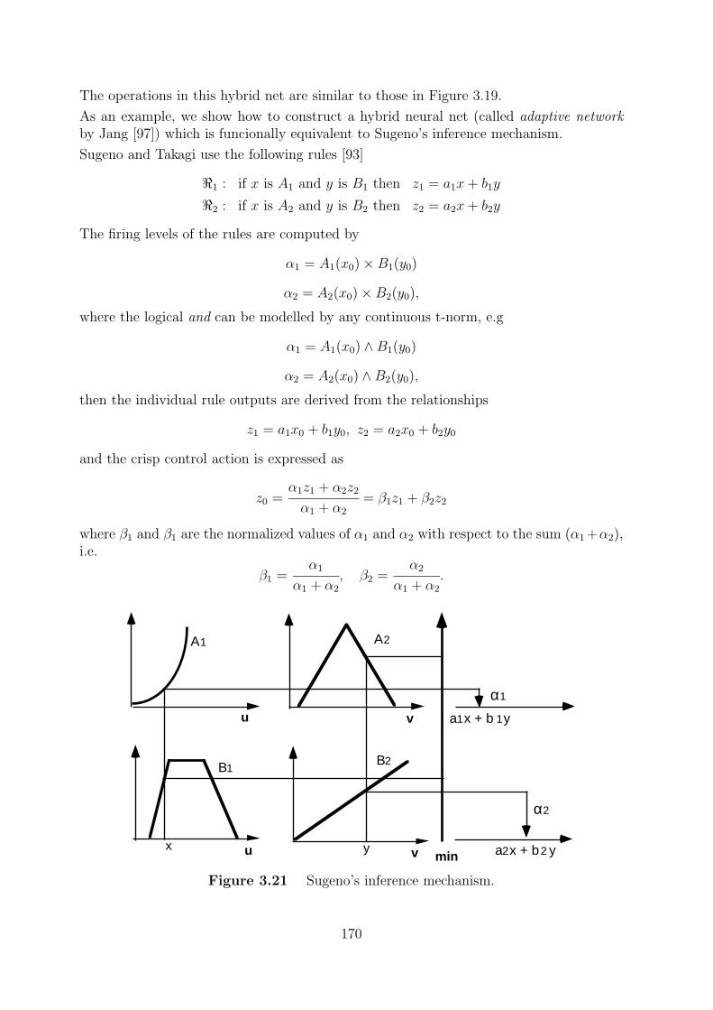
u v
u v min
α1
α2
A1
B1
A2
B2
a1x + b 1y
a2x + b2 yx y
The operations in this hybrid net are similar to those in Figure 3.19.
As an example, we show how to construct a hybrid neural net (called adaptive networkby Jang [97]) which is funcionally equivalent to Sugeno’s inference mechanism.
Sugeno and Takagi use the following rules [93]
<1 : if x is A1 and y is B1 then z1 = a1x+ b1y
<2 : if x is A2 and y is B2 then z2 = a2x+ b2y
The firing levels of the rules are computed by
α1 = A1(x0)×B1(y0)
α2 = A2(x0)×B2(y0),
where the logical and can be modelled by any continuous t-norm, e.g
α1 = A1(x0) ∧B1(y0)
α2 = A2(x0) ∧B2(y0),
then the individual rule outputs are derived from the relationships
z1 = a1x0 + b1y0, z2 = a2x0 + b2y0
and the crisp control action is expressed as
z0 =α1z1 + α2z2
α1 + α2
= β1z1 + β2z2
where β1 and β1 are the normalized values of α1 and α2 with respect to the sum (α1 +α2),i.e.
β1 =α1
α1 + α2
, β2 =α2
α1 + α2
.
Figure 3.21 Sugeno’s inference mechanism.
170
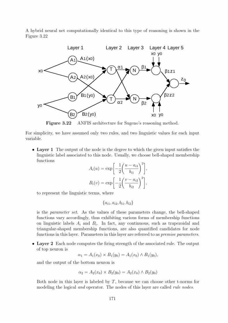
A1
A2
B1
B2
A1(x0)
A2(x0)
B1(y0)
B2(y0)
α1
α2
T
T
N
N
β1
β2
β1z1
β2z2
z0
Layer 1 Layer 2 Layer 3 Layer 4 Layer 5
x0
y0
x0
x0 y0
y0
A hybrid neural net computationally identical to this type of reasoning is shown in theFigure 3.22
Figure 3.22 ANFIS architecture for Sugeno’s reasoning method.
For simplicity, we have assumed only two rules, and two linguistic values for each inputvariable.
• Layer 1 The output of the node is the degree to which the given input satisfies thelinguistic label associated to this node. Usually, we choose bell-shaped membershipfunctions
Ai(u) = exp
[−
1
2
(u− ai1bi1
)2],
Bi(v) = exp
[−
1
2
(v − ai2bi2
)2],
to represent the linguistic terms, where
{ai1, ai2, bi1, bi2}
is the parameter set. As the values of these parameters change, the bell-shapedfunctions vary accordingly, thus exhibiting various forms of membership functionson linguistic labels Ai and Bi. In fact, any continuous, such as trapezoidal andtriangular-shaped membership functions, are also quantified candidates for nodefunctions in this layer. Parameters in this layer are referred to as premise parameters.
• Layer 2 Each node computes the firing strength of the associated rule. The outputof top neuron is
α1 = A1(x0)×B1(y0) = A1(x0) ∧B1(y0),
and the output of the bottom neuron is
α2 = A2(x0)×B2(y0) = A2(x0) ∧B2(y0)
Both node in this layer is labeled by T , because we can choose other t-norms formodeling the logical and operator. The nodes of this layer are called rule nodes.
171
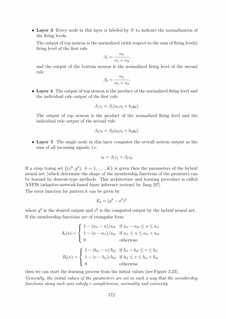
• Layer 3 Every node in this layer is labeled by N to indicate the normalization ofthe firing levels.
The output of top neuron is the normalized (with respect to the sum of firing levels)firing level of the first rule
β1 =α1
α1 + α2
,
and the output of the bottom neuron is the normalized firing level of the secondrule
β2 =α2
α1 + α2
,
• Layer 4 The output of top neuron is the product of the normalized firing level andthe individual rule output of the first rule
β1z1 = β1(a1x0 + b1y0),
The output of top neuron is the product of the normalized firing level and theindividual rule output of the second rule
β2z2 = β2(a2x0 + b2y0),
• Layer 5 The single node in this layer computes the overall system output as thesum of all incoming signals, i.e.
z0 = β1z1 + β2z2.
If a crisp traing set {(xk, yk), k = 1, . . . , K} is given then the parameters of the hybridneural net (which determine the shape of the membership functions of the premises) canbe learned by descent-type methods. This architecture and learning procedure is calledANFIS (adaptive-network-based fuzzy inference system) by Jang [97].
The error function for pattern k can be given by
Ek = (yk − ok)2
where yk is the desired output and ok is the computed output by the hybrid neural net.
If the membership functions are of triangular form
Ai(u) =
1− (ai1 − u)/ai2 if ai1 − ai2 ≤ u ≤ ai1
1− (u− ai1)/ai3 if ai1 ≤ u ≤ ai1 + ai3
0 otherwise
Bi(v) =
1− (bi1 − v)/bi2 if bi1 − bi2 ≤ v ≤ bi1
1− (v − bi1)/bi3 if bi1 ≤ v ≤ bi1 + bi3
0 otherwise
then we can start the learning process from the initial values (see Figure 3.23).
Generally, the initial values of the parameters are set in such a way that the membershipfunctions along each axis satisfy ε-completeness, normality and convexity.
172
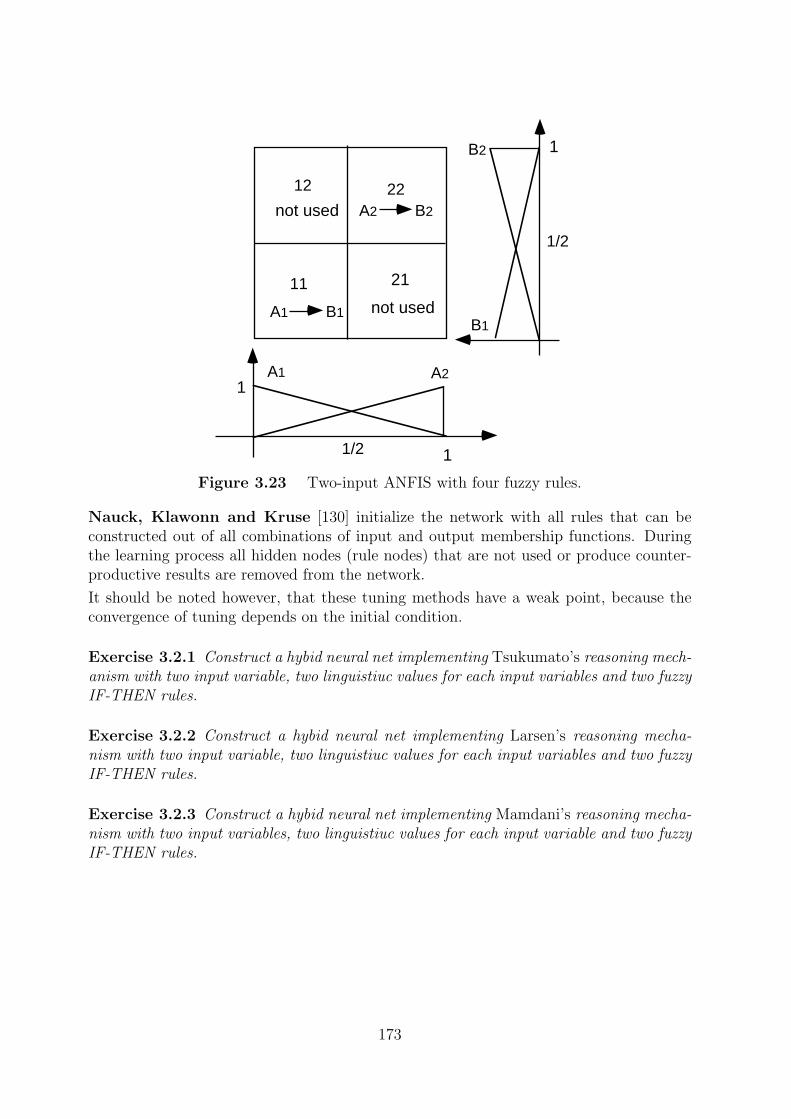
A1 A2
B1
B2
1
1
1
1/2
1/2
11
12 22
21
A1 B1 not used
not used A2 B2
Figure 3.23 Two-input ANFIS with four fuzzy rules.
Nauck, Klawonn and Kruse [130] initialize the network with all rules that can beconstructed out of all combinations of input and output membership functions. Duringthe learning process all hidden nodes (rule nodes) that are not used or produce counter-productive results are removed from the network.
It should be noted however, that these tuning methods have a weak point, because theconvergence of tuning depends on the initial condition.
Exercise 3.2.1 Construct a hybid neural net implementing Tsukumato’s reasoning mech-anism with two input variable, two linguistiuc values for each input variables and two fuzzyIF-THEN rules.
Exercise 3.2.2 Construct a hybid neural net implementing Larsen’s reasoning mecha-nism with two input variable, two linguistiuc values for each input variables and two fuzzyIF-THEN rules.
Exercise 3.2.3 Construct a hybid neural net implementing Mamdani’s reasoning mecha-nism with two input variables, two linguistiuc values for each input variable and two fuzzyIF-THEN rules.
173
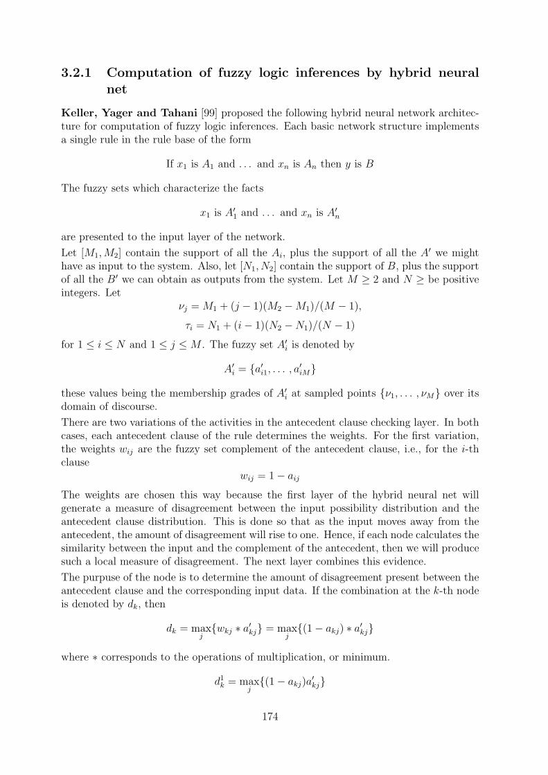
3.2.1 Computation of fuzzy logic inferences by hybrid neuralnet
Keller, Yager and Tahani [99] proposed the following hybrid neural network architec-ture for computation of fuzzy logic inferences. Each basic network structure implementsa single rule in the rule base of the form
If x1 is A1 and . . . and xn is An then y is B
The fuzzy sets which characterize the facts
x1 is A′1 and . . . and xn is A′n
are presented to the input layer of the network.
Let [M1,M2] contain the support of all the Ai, plus the support of all the A′ we mighthave as input to the system. Also, let [N1, N2] contain the support of B, plus the supportof all the B′ we can obtain as outputs from the system. Let M ≥ 2 and N ≥ be positiveintegers. Let
νj = M1 + (j − 1)(M2 −M1)/(M − 1),
τi = N1 + (i− 1)(N2 −N1)/(N − 1)
for 1 ≤ i ≤ N and 1 ≤ j ≤M . The fuzzy set A′i is denoted by
A′i = {a′i1, . . . , a′iM}
these values being the membership grades of A′i at sampled points {ν1, . . . , νM} over itsdomain of discourse.
There are two variations of the activities in the antecedent clause checking layer. In bothcases, each antecedent clause of the rule determines the weights. For the first variation,the weights wij are the fuzzy set complement of the antecedent clause, i.e., for the i-thclause
wij = 1− aijThe weights are chosen this way because the first layer of the hybrid neural net willgenerate a measure of disagreement between the input possibility distribution and theantecedent clause distribution. This is done so that as the input moves away from theantecedent, the amount of disagreement will rise to one. Hence, if each node calculates thesimilarity between the input and the complement of the antecedent, then we will producesuch a local measure of disagreement. The next layer combines this evidence.
The purpuse of the node is to determine the amount of disagreement present between theantecedent clause and the corresponding input data. If the combination at the k-th nodeis denoted by dk, then
dk = maxj{wkj ∗ a′kj} = max
j{(1− akj) ∗ a′kj}
where ∗ corresponds to the operations of multiplication, or minimum.
d1k = max
j{(1− akj)a′kj}
174
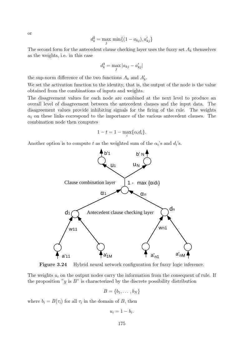
u1
d1dn
αnα1
b'1 b' N
a'11
w11 wn1
Clause combination layer
Antecedent clause checking layer
1 - max {αidi}
uN
a'1M a'nMa'n1
ord2k = max
jmin{(1− akj), a′kj}
The second form for the antecedent clause checking layer uses the fuzzy set Ak themselvesas the weights, i.e. in this case
d3k = max
j|akj − a′kj|
the sup-norm difference of the two functions Ak and A′k.
We set the activation function to the identity, that is, the output of the node is the valueobtained from the combinations of inputs and weights.
The disagreement values for each node are combined at the next level to produce anoverall level of disagreement between the antecedent clauses and the input data. Thedisagreement values provide inhibiting signals for the firing of the rule. The weightsαi on these links correspond to the importance of the various antecedent clauses. Thecombination node then computes
1− t = 1−maxi{αidi}.
Another option is to compute t as the weighted sum of the αi’s and di’s.
Figure 3.24 Hybrid neural network configuration for fuzzy logic inference.
The weights ui on the output nodes carry the information from the consequent of rule. Ifthe proposition ”y is B” is characterized by the discrete possibility distribution
B = {b1, . . . , bN}
where bi = B(τi) for all τi in the domain of B, then
ui = 1− bi.
175
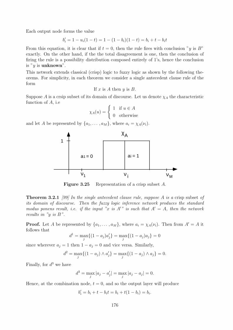
ν ν
χΑ
M1
1
ν i
ai = 1 a1 = 0
Each output node forms the value
b′i = 1− ui(1− t) = 1− (1− bi)(1− t) = bi + t− bitFrom this equation, it is clear that if t = 0, then the rule fires with conclusion ”y is B”exactly. On the other hand, if the the total disagreement is one, then the conclusion offiring the rule is a possibility distribution composed entirely of 1’s, hence the conclusionis ”y is unknown”.
This network extends classical (crisp) logic to fuzzy logic as shown by the following the-orems. For simplicity, in each theorem we consider a single antecedent clause rule of theform
If x is A then y is B.
Suppose A is a crsip subset of its domain of discourse. Let us denote χA the characteristicfunction of A, i.e
χA(u) =
{1 if u ∈ A0 otherwise
and let A be represented by {a1, . . . , aM}, where ai = χA(νi).
Figure 3.25 Representation of a crisp subset A.
Theorem 3.2.1 [99] In the single antecedent clause rule, suppose A is a crisp subset ofits domain of discourse. Then the fuzzy logic inference network produces the standardmodus ponens result, i.e. if the input ”x is A′” is such that A′ = A, then the networkresults in ”y is B”.
Proof. Let A be represented by {a1, . . . , aM}, where ai = χA(νi). Then from A′ = A itfollows that
d1 = maxj{(1− aj)a′j} = max
j{(1− aj)aj} = 0
since wherever aj = 1 then 1− aj = 0 and vice versa. Similarly,
d2 = maxj{(1− aj) ∧ a′j} = max
j{(1− aj) ∧ aj} = 0.
Finally, for d3 we have
d3 = maxj|aj − a′j| = max
j|aj − aj| = 0.
Hence, at the combination node, t = 0, and so the output layer will produce
b′i = bi + t− bit = bi + t(1− bi) = bi.
176
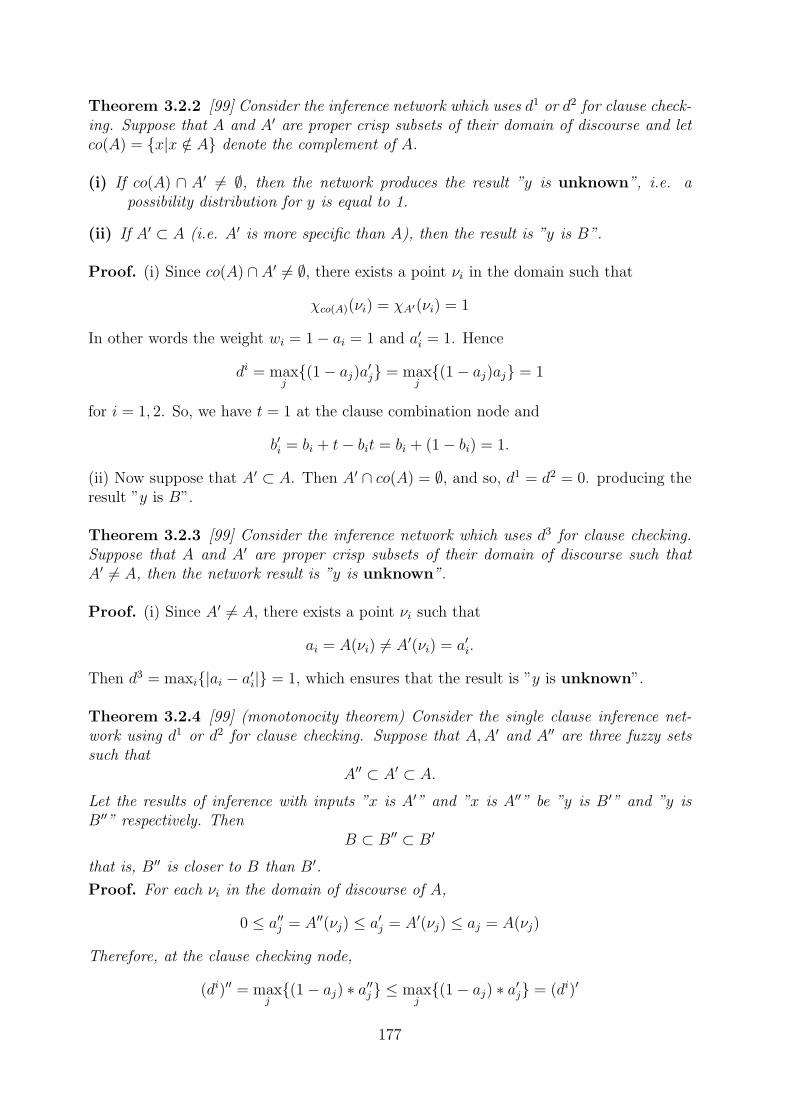
Theorem 3.2.2 [99] Consider the inference network which uses d1 or d2 for clause check-ing. Suppose that A and A′ are proper crisp subsets of their domain of discourse and letco(A) = {x|x /∈ A} denote the complement of A.
(i) If co(A) ∩ A′ 6= ∅, then the network produces the result ”y is unknown”, i.e. apossibility distribution for y is equal to 1.
(ii) If A′ ⊂ A (i.e. A′ is more specific than A), then the result is ”y is B”.
Proof. (i) Since co(A) ∩ A′ 6= ∅, there exists a point νi in the domain such that
χco(A)(νi) = χA′(νi) = 1
In other words the weight wi = 1− ai = 1 and a′i = 1. Hence
di = maxj{(1− aj)a′j} = max
j{(1− aj)aj} = 1
for i = 1, 2. So, we have t = 1 at the clause combination node and
b′i = bi + t− bit = bi + (1− bi) = 1.
(ii) Now suppose that A′ ⊂ A. Then A′ ∩ co(A) = ∅, and so, d1 = d2 = 0. producing theresult ”y is B”.
Theorem 3.2.3 [99] Consider the inference network which uses d3 for clause checking.Suppose that A and A′ are proper crisp subsets of their domain of discourse such thatA′ 6= A, then the network result is ”y is unknown”.
Proof. (i) Since A′ 6= A, there exists a point νi such that
ai = A(νi) 6= A′(νi) = a′i.
Then d3 = maxi{|ai − a′i|} = 1, which ensures that the result is ”y is unknown”.
Theorem 3.2.4 [99] (monotonocity theorem) Consider the single clause inference net-work using d1 or d2 for clause checking. Suppose that A,A′ and A′′ are three fuzzy setssuch that
A′′ ⊂ A′ ⊂ A.
Let the results of inference with inputs ”x is A′” and ”x is A′′” be ”y is B′” and ”y isB′′” respectively. Then
B ⊂ B′′ ⊂ B′
that is, B′′ is closer to B than B′.
Proof. For each νi in the domain of discourse of A,
0 ≤ a′′j = A′′(νj) ≤ a′j = A′(νj) ≤ aj = A(νj)
Therefore, at the clause checking node,
(di)′′ = maxj{(1− aj) ∗ a′′j} ≤ max
j{(1− aj) ∗ a′j} = (di)′
177
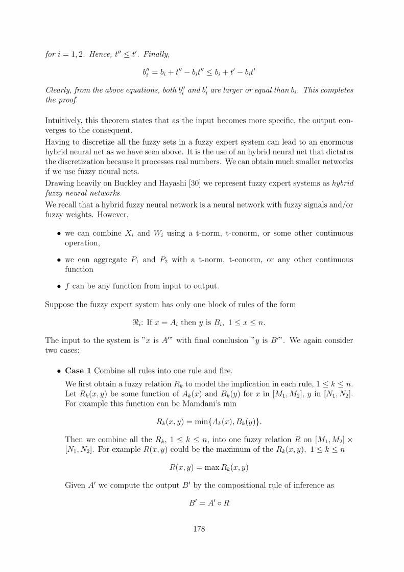
for i = 1, 2. Hence, t′′ ≤ t′. Finally,
b′′i = bi + t′′ − bit′′ ≤ bi + t′ − bit′
Clearly, from the above equations, both b′′i and b′i are larger or equal than bi. This completesthe proof.
Intuitively, this theorem states that as the input becomes more specific, the output con-verges to the consequent.
Having to discretize all the fuzzy sets in a fuzzy expert system can lead to an enormoushybrid neural net as we have seen above. It is the use of an hybrid neural net that dictatesthe discretization because it processes real numbers. We can obtain much smaller networksif we use fuzzy neural nets.
Drawing heavily on Buckley and Hayashi [30] we represent fuzzy expert systems as hybridfuzzy neural networks.
We recall that a hybrid fuzzy neural network is a neural network with fuzzy signals and/orfuzzy weights. However,
• we can combine Xi and Wi using a t-norm, t-conorm, or some other continuousoperation,
• we can aggregate P1 and P2 with a t-norm, t-conorm, or any other continuousfunction
• f can be any function from input to output.
Suppose the fuzzy expert system has only one block of rules of the form
<i: If x = Ai then y is Bi, 1 ≤ x ≤ n.
The input to the system is ”x is A′” with final conclusion ”y is B′”. We again considertwo cases:
• Case 1 Combine all rules into one rule and fire.
We first obtain a fuzzy relation Rk to model the implication in each rule, 1 ≤ k ≤ n.Let Rk(x, y) be some function of Ak(x) and Bk(y) for x in [M1,M2], y in [N1, N2].For example this function can be Mamdani’s min
Rk(x, y) = min{Ak(x), Bk(y)}.
Then we combine all the Rk, 1 ≤ k ≤ n, into one fuzzy relation R on [M1,M2] ×[N1, N2]. For example R(x, y) could be the maximum of the Rk(x, y), 1 ≤ k ≤ n
R(x, y) = maxRk(x, y)
Given A′ we compute the output B′ by the compositional rule of inference as
B′ = A′ ◦R
178
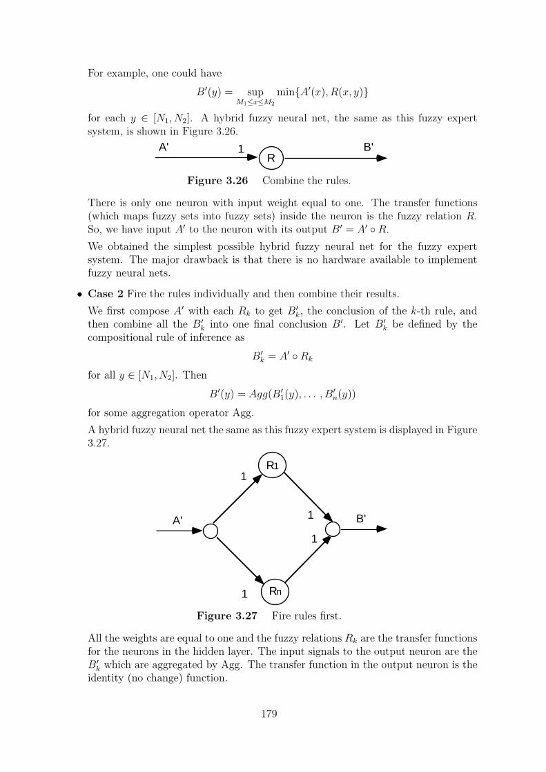
A' 1 B'R
A'
R1
Rn
B'
1
1
1
1
For example, one could have
B′(y) = supM1≤x≤M2
min{A′(x), R(x, y)}
for each y ∈ [N1, N2]. A hybrid fuzzy neural net, the same as this fuzzy expertsystem, is shown in Figure 3.26.
Figure 3.26 Combine the rules.
There is only one neuron with input weight equal to one. The transfer functions(which maps fuzzy sets into fuzzy sets) inside the neuron is the fuzzy relation R.So, we have input A′ to the neuron with its output B′ = A′ ◦R.
We obtained the simplest possible hybrid fuzzy neural net for the fuzzy expertsystem. The major drawback is that there is no hardware available to implementfuzzy neural nets.
• Case 2 Fire the rules individually and then combine their results.
We first compose A′ with each Rk to get B′k, the conclusion of the k-th rule, andthen combine all the B′k into one final conclusion B′. Let B′k be defined by thecompositional rule of inference as
B′k = A′ ◦Rk
for all y ∈ [N1, N2]. Then
B′(y) = Agg(B′1(y), . . . , B′n(y))
for some aggregation operator Agg.
A hybrid fuzzy neural net the same as this fuzzy expert system is displayed in Figure3.27.
Figure 3.27 Fire rules first.
All the weights are equal to one and the fuzzy relations Rk are the transfer functionsfor the neurons in the hidden layer. The input signals to the output neuron are theB′k which are aggregated by Agg. The transfer function in the output neuron is theidentity (no change) function.
179
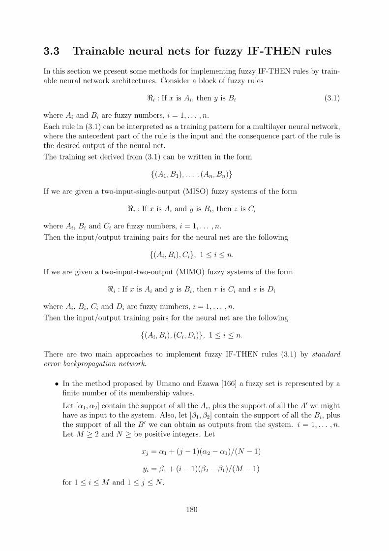
3.3 Trainable neural nets for fuzzy IF-THEN rules
In this section we present some methods for implementing fuzzy IF-THEN rules by train-able neural network architectures. Consider a block of fuzzy rules
<i : If x is Ai, then y is Bi (3.1)
where Ai and Bi are fuzzy numbers, i = 1, . . . , n.
Each rule in (3.1) can be interpreted as a training pattern for a multilayer neural network,where the antecedent part of the rule is the input and the consequence part of the rule isthe desired output of the neural net.
The training set derived from (3.1) can be written in the form
{(A1, B1), . . . , (An, Bn)}
If we are given a two-input-single-output (MISO) fuzzy systems of the form
<i : If x is Ai and y is Bi, then z is Ci
where Ai, Bi and Ci are fuzzy numbers, i = 1, . . . , n.
Then the input/output training pairs for the neural net are the following
{(Ai, Bi), Ci}, 1 ≤ i ≤ n.
If we are given a two-input-two-output (MIMO) fuzzy systems of the form
<i : If x is Ai and y is Bi, then r is Ci and s is Di
where Ai, Bi, Ci and Di are fuzzy numbers, i = 1, . . . , n.
Then the input/output training pairs for the neural net are the following
{(Ai, Bi), (Ci, Di)}, 1 ≤ i ≤ n.
There are two main approaches to implement fuzzy IF-THEN rules (3.1) by standarderror backpropagation network.
• In the method proposed by Umano and Ezawa [166] a fuzzy set is represented by afinite number of its membership values.
Let [α1, α2] contain the support of all the Ai, plus the support of all the A′ we mighthave as input to the system. Also, let [β1, β2] contain the support of all the Bi, plusthe support of all the B′ we can obtain as outputs from the system. i = 1, . . . , n.Let M ≥ 2 and N ≥ be positive integers. Let
xj = α1 + (j − 1)(α2 − α1)/(N − 1)
yi = β1 + (i− 1)(β2 − β1)/(M − 1)
for 1 ≤ i ≤M and 1 ≤ j ≤ N .
180
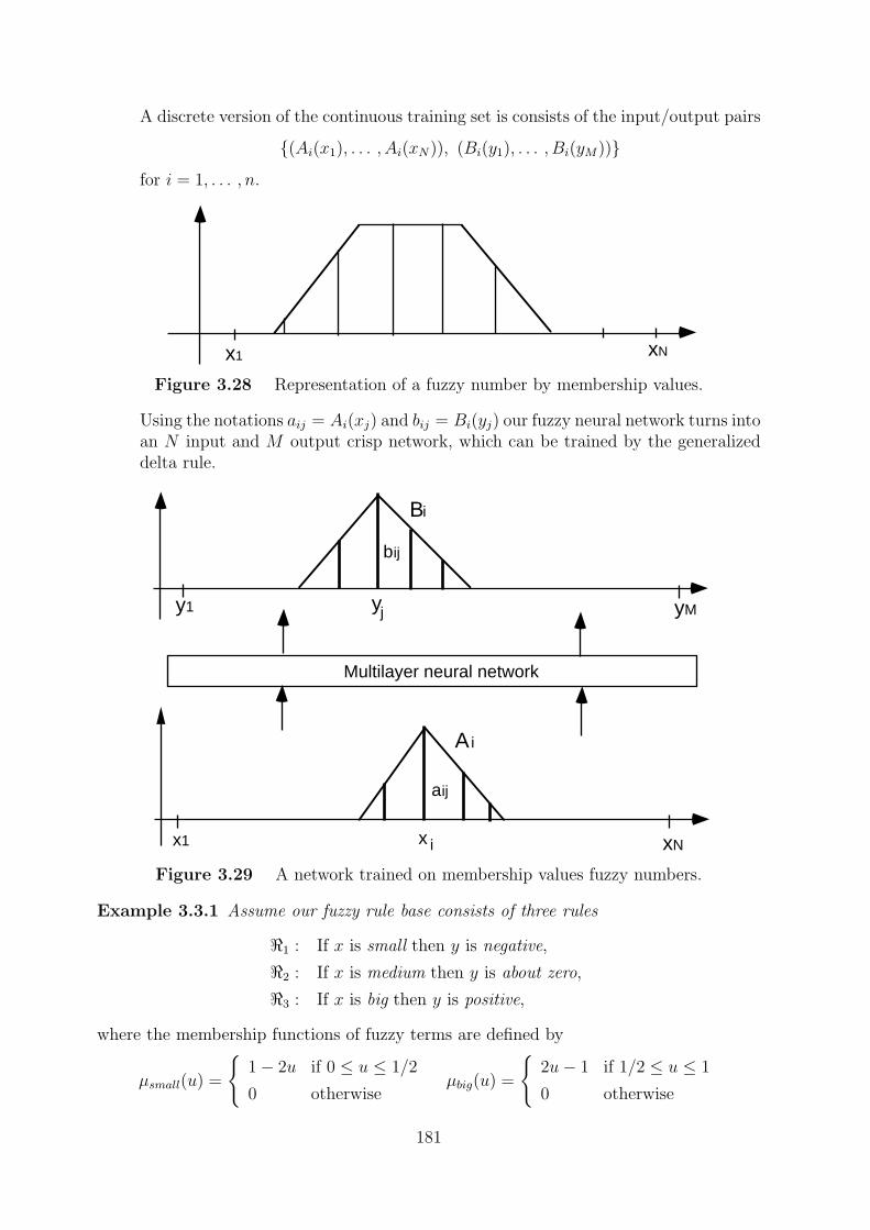
x1 xN
x1
y1 yM
xN
Ai
Bi
aij
bij
y
Multilayer neural network
j
x i
A discrete version of the continuous training set is consists of the input/output pairs
{(Ai(x1), . . . , Ai(xN)), (Bi(y1), . . . , Bi(yM))}for i = 1, . . . , n.
Figure 3.28 Representation of a fuzzy number by membership values.
Using the notations aij = Ai(xj) and bij = Bi(yj) our fuzzy neural network turns intoan N input and M output crisp network, which can be trained by the generalizeddelta rule.
Figure 3.29 A network trained on membership values fuzzy numbers.
Example 3.3.1 Assume our fuzzy rule base consists of three rules
<1 : If x is small then y is negative,
<2 : If x is medium then y is about zero,
<3 : If x is big then y is positive,
where the membership functions of fuzzy terms are defined by
µsmall(u) =
{1− 2u if 0 ≤ u ≤ 1/2
0 otherwiseµbig(u) =
{2u− 1 if 1/2 ≤ u ≤ 1
0 otherwise
181
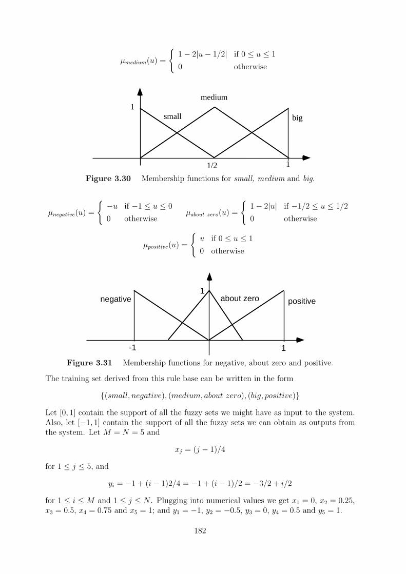
1small
medium
big
11/2
1
1
negative positiveabout zero
-1
µmedium(u) =
{1− 2|u− 1/2| if 0 ≤ u ≤ 1
0 otherwise
Figure 3.30 Membership functions for small, medium and big.
µnegative(u) =
{−u if −1 ≤ u ≤ 0
0 otherwiseµabout zero(u) =
{1− 2|u| if −1/2 ≤ u ≤ 1/2
0 otherwise
µpositive(u) =
{u if 0 ≤ u ≤ 1
0 otherwise
Figure 3.31 Membership functions for negative, about zero and positive.
The training set derived from this rule base can be written in the form
{(small, negative), (medium, about zero), (big, positive)}
Let [0, 1] contain the support of all the fuzzy sets we might have as input to the system.Also, let [−1, 1] contain the support of all the fuzzy sets we can obtain as outputs fromthe system. Let M = N = 5 and
xj = (j − 1)/4
for 1 ≤ j ≤ 5, and
yi = −1 + (i− 1)2/4 = −1 + (i− 1)/2 = −3/2 + i/2
for 1 ≤ i ≤ M and 1 ≤ j ≤ N . Plugging into numerical values we get x1 = 0, x2 = 0.25,x3 = 0.5, x4 = 0.75 and x5 = 1; and y1 = −1, y2 = −0.5, y3 = 0, y4 = 0.5 and y5 = 1.
182
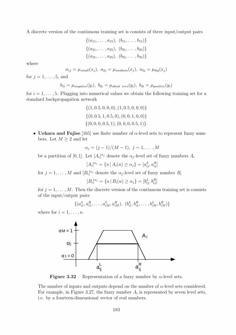
αΜ = 1
α j
α1 = 0
Ai
aij a ijL R
A discrete version of the continuous training set is consists of three input/output pairs
{(a11, . . . , a15), (b11, . . . , b15)}{(a21, . . . , a25), (b21, . . . , b25)}{(a31, . . . , a35), (b31, . . . , b35)}
wherea1j = µsmall(xj), a2j = µmedium(xj), a3j = µbig(xj)
for j = 1, . . . , 5, and
b1i = µnegative(yi), b2i = µabout zero(yi), b3i = µpositive(yi)
for i = 1, . . . , 5. Plugging into numerical values we obtain the following training set for astandard backpropagation network
{(1, 0.5, 0, 0, 0), (1, 0.5, 0, 0, 0)}{(0, 0.5, 1, 0.5, 0), (0, 0, 1, 0, 0)}{(0, 0, 0, 0.5, 1), (0, 0, 0, 0.5, 1)}.
• Uehara and Fujise [165] use finite number of α-level sets to represent fuzzy num-bers. Let M ≥ 2 and let
αj = (j − 1)/(M − 1), j = 1, . . . ,M
be a partition of [0, 1]. Let [Ai]αj denote the αj-level set of fuzzy numbers Ai
[Ai]αj = {u |Ai(u) ≥ αj} = [aLij, a
Rij]
for j = 1, . . . ,M and [Bi]αj denote the αj-level set of fuzzy number Bi
[Bi]αj = {u |Bi(u) ≥ αj} = [bLij, b
Rij]
for j = 1, . . . ,M . Then the discrete version of the continuous training set is consistsof the input/output pairs
{(aLi1, aRi1, . . . , aLiM , aRiM), (bLi1, bRi1, . . . , b
LiM , b
RiM)}
where for i = 1, . . . , n.
Figure 3.32 Representation of a fuzzy number by α-level sets.
The number of inputs and outputs depend on the number of α-level sets considered.For example, in Figure 3.27, the fuzzy number Ai is represented by seven level sets,i.e. by a fourteen-dimensional vector of real numbers.
183
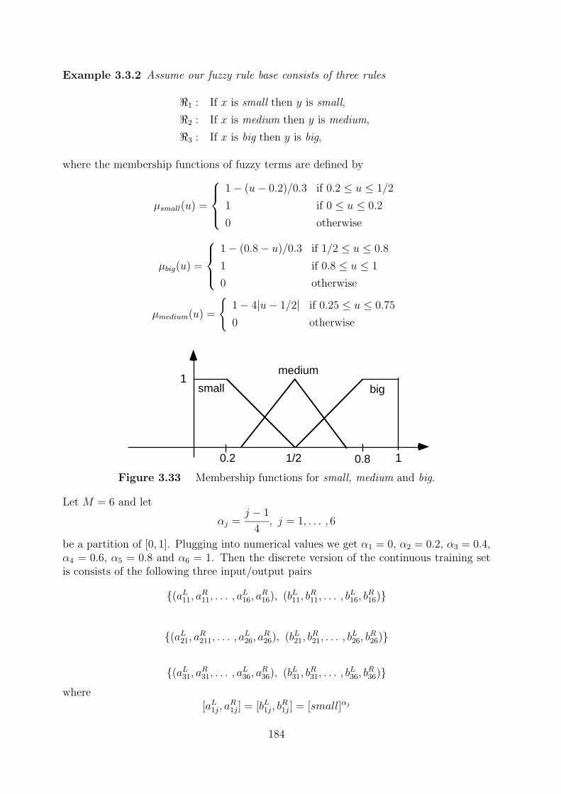
1small
medium
big
11/20.2 0.8
Example 3.3.2 Assume our fuzzy rule base consists of three rules
<1 : If x is small then y is small,
<2 : If x is medium then y is medium,
<3 : If x is big then y is big,
where the membership functions of fuzzy terms are defined by
µsmall(u) =
1− (u− 0.2)/0.3 if 0.2 ≤ u ≤ 1/2
1 if 0 ≤ u ≤ 0.2
0 otherwise
µbig(u) =
1− (0.8− u)/0.3 if 1/2 ≤ u ≤ 0.8
1 if 0.8 ≤ u ≤ 1
0 otherwise
µmedium(u) =
{1− 4|u− 1/2| if 0.25 ≤ u ≤ 0.75
0 otherwise
Figure 3.33 Membership functions for small, medium and big.
Let M = 6 and let
αj =j − 1
4, j = 1, . . . , 6
be a partition of [0, 1]. Plugging into numerical values we get α1 = 0, α2 = 0.2, α3 = 0.4,α4 = 0.6, α5 = 0.8 and α6 = 1. Then the discrete version of the continuous training setis consists of the following three input/output pairs
{(aL11, aR11, . . . , a
L16, a
R16), (bL11, b
R11, . . . , b
L16, b
R16)}
{(aL21, aR211, . . . , a
L26, a
R26), (bL21, b
R21, . . . , b
L26, b
R26)}
{(aL31, aR31, . . . , a
L36, a
R36), (bL31, b
R31, . . . , b
L36, b
R36)}
where[aL1j, a
R1j] = [bL1j, b
R1j] = [small]αj
184
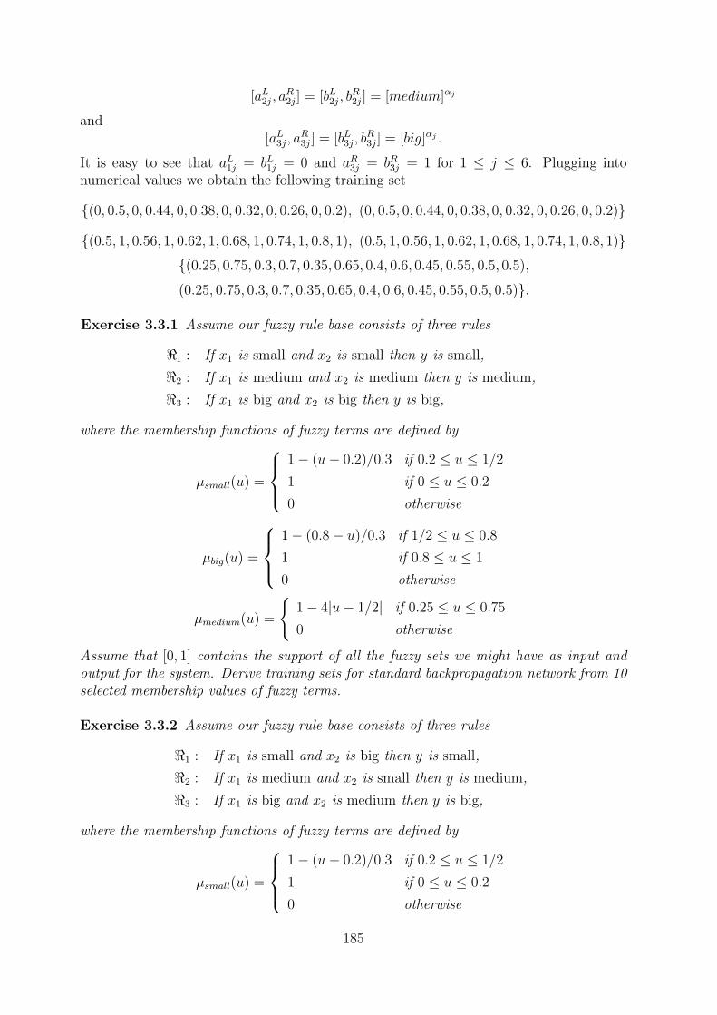
[aL2j, aR2j] = [bL2j, b
R2j] = [medium]αj
and[aL3j, a
R3j] = [bL3j, b
R3j] = [big]αj .
It is easy to see that aL1j = bL1j = 0 and aR3j = bR3j = 1 for 1 ≤ j ≤ 6. Plugging intonumerical values we obtain the following training set
{(0, 0.5, 0, 0.44, 0, 0.38, 0, 0.32, 0, 0.26, 0, 0.2), (0, 0.5, 0, 0.44, 0, 0.38, 0, 0.32, 0, 0.26, 0, 0.2)}
{(0.5, 1, 0.56, 1, 0.62, 1, 0.68, 1, 0.74, 1, 0.8, 1), (0.5, 1, 0.56, 1, 0.62, 1, 0.68, 1, 0.74, 1, 0.8, 1)}{(0.25, 0.75, 0.3, 0.7, 0.35, 0.65, 0.4, 0.6, 0.45, 0.55, 0.5, 0.5),
(0.25, 0.75, 0.3, 0.7, 0.35, 0.65, 0.4, 0.6, 0.45, 0.55, 0.5, 0.5)}.
Exercise 3.3.1 Assume our fuzzy rule base consists of three rules
<1 : If x1 is small and x2 is small then y is small,
<2 : If x1 is medium and x2 is medium then y is medium,
<3 : If x1 is big and x2 is big then y is big,
where the membership functions of fuzzy terms are defined by
µsmall(u) =
1− (u− 0.2)/0.3 if 0.2 ≤ u ≤ 1/2
1 if 0 ≤ u ≤ 0.2
0 otherwise
µbig(u) =
1− (0.8− u)/0.3 if 1/2 ≤ u ≤ 0.8
1 if 0.8 ≤ u ≤ 1
0 otherwise
µmedium(u) =
{1− 4|u− 1/2| if 0.25 ≤ u ≤ 0.75
0 otherwise
Assume that [0, 1] contains the support of all the fuzzy sets we might have as input andoutput for the system. Derive training sets for standard backpropagation network from 10selected membership values of fuzzy terms.
Exercise 3.3.2 Assume our fuzzy rule base consists of three rules
<1 : If x1 is small and x2 is big then y is small,
<2 : If x1 is medium and x2 is small then y is medium,
<3 : If x1 is big and x2 is medium then y is big,
where the membership functions of fuzzy terms are defined by
µsmall(u) =
1− (u− 0.2)/0.3 if 0.2 ≤ u ≤ 1/2
1 if 0 ≤ u ≤ 0.2
0 otherwise
185
µbig(u) =
1− (0.8− u)/0.3 if 1/2 ≤ u ≤ 0.8
1 if 0.8 ≤ u ≤ 1
0 otherwise
µmedium(u) =
{1− 4|u− 1/2| if 0.25 ≤ u ≤ 0.75
0 otherwise
Assume that [0, 1] contains the support of all the fuzzy sets we might have as input andoutput for the system. Derive training sets for standard backpropagation network from 10selected values of α-level sets of fuzzy terms.
186
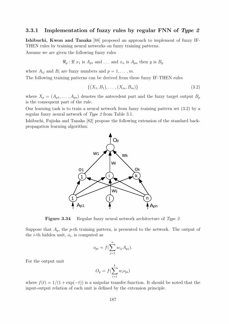
wij
wi
Οp
wkw1
Ap1 Apn
1 i k
1 j n
οkο1
3.3.1 Implementation of fuzzy rules by regular FNN of Type 2
Ishibuchi, Kwon and Tanaka [88] proposed an approach to implement of fuzzy IF-THEN rules by training neural networks on fuzzy training patterns.
Assume we are given the following fuzzy rules
<p : If x1 is Ap1 and . . . and xn is Apn then y is Bp
where Aij and Bi are fuzzy numbers and p = 1, . . . ,m.
The following training patterns can be derived from these fuzzy IF-THEN rules
{(X1, B1), . . . , (Xm, Bm)} (3.2)
where Xp = (Ap1, . . . , Apn) denotes the antecedent part and the fuzzy target output Bp
is the consequent part of the rule.
Our learning task is to train a neural network from fuzzy training pattern set (3.2) by aregular fuzzy neural network of Type 2 from Table 3.1.
Ishibuchi, Fujioka and Tanaka [82] propose the following extension of the standard back-propagation learning algorithm:
Figure 3.34 Regular fuzzy neural network architecture of Type 2.
Suppose that Ap, the p-th training pattern, is presented to the network. The output ofthe i-th hidden unit, oi, is computed as
opi = f(n∑j=1
wijApj).
For the output unit
Op = f(k∑i=1
wiopi)
where f(t) = 1/(1 + exp(−t)) is a unipolar transfer function. It should be noted that theinput-output relation of each unit is defined by the extension principle.
187
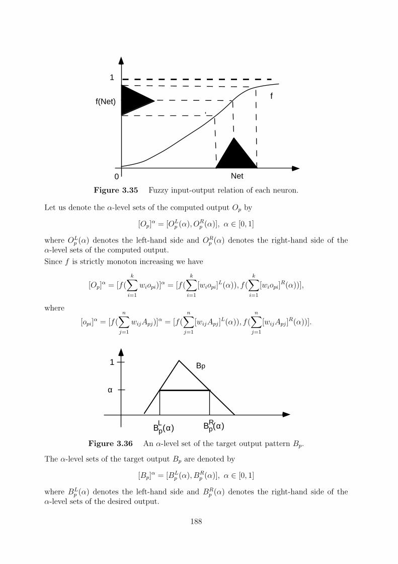
Net
f(Net)
0
1
f
α
Bp
B (α) L B (α) R
1
p p
Figure 3.35 Fuzzy input-output relation of each neuron.
Let us denote the α-level sets of the computed output Op by
[Op]α = [OL
p (α), ORp (α)], α ∈ [0, 1]
where OLp (α) denotes the left-hand side and OR
p (α) denotes the right-hand side of theα-level sets of the computed output.
Since f is strictly monoton increasing we have
[Op]α = [f(
k∑i=1
wiopi)]α = [f(
k∑i=1
[wiopi]L(α)), f(
k∑i=1
[wiopi]R(α))],
where
[opi]α = [f(
n∑j=1
wijApj)]α = [f(
n∑j=1
[wijApj]L(α)), f(
n∑j=1
[wijApj]R(α))].
Figure 3.36 An α-level set of the target output pattern Bp.
The α-level sets of the target output Bp are denoted by
[Bp]α = [BL
p (α), BRp (α)], α ∈ [0, 1]
where BLp (α) denotes the left-hand side and BR
p (α) denotes the right-hand side of theα-level sets of the desired output.
188
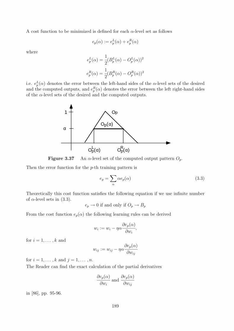
α
Οp
Ο (α)
1
p
Ο (α) p Ο (α) pL R
A cost function to be minimized is defined for each α-level set as follows
ep(α) := eLp (α) + eRp (α)
where
eLp (α) =1
2(BL
p (α)−OLp (α))2
eRp (α) =1
2(BR
p (α)−ORp (α))2
i.e. eLp (α) denotes the error between the left-hand sides of the α-level sets of the desiredand the computed outputs, and eRp (α) denotes the error between the left right-hand sidesof the α-level sets of the desired and the computed outputs.
Figure 3.37 An α-level set of the computed output pattern Op.
Then the error function for the p-th training pattern is
ep =∑α
αep(α) (3.3)
Theoretically this cost function satisfies the following equation if we use infinite numberof α-level sets in (3.3).
ep → 0 if and only if Op → Bp
From the cost function ep(α) the following learning rules can be derived
wi := wi − ηα∂ep(α)
∂wi,
for i = 1, . . . , k and
wij := wij − ηα∂ep(α)
∂wij
for i = 1, . . . , k and j = 1, . . . , n.
The Reader can find the exact calculation of the partial derivatives
∂ep(α)
∂wiand
∂ep(α)
∂wij
in [86], pp. 95-96.
189
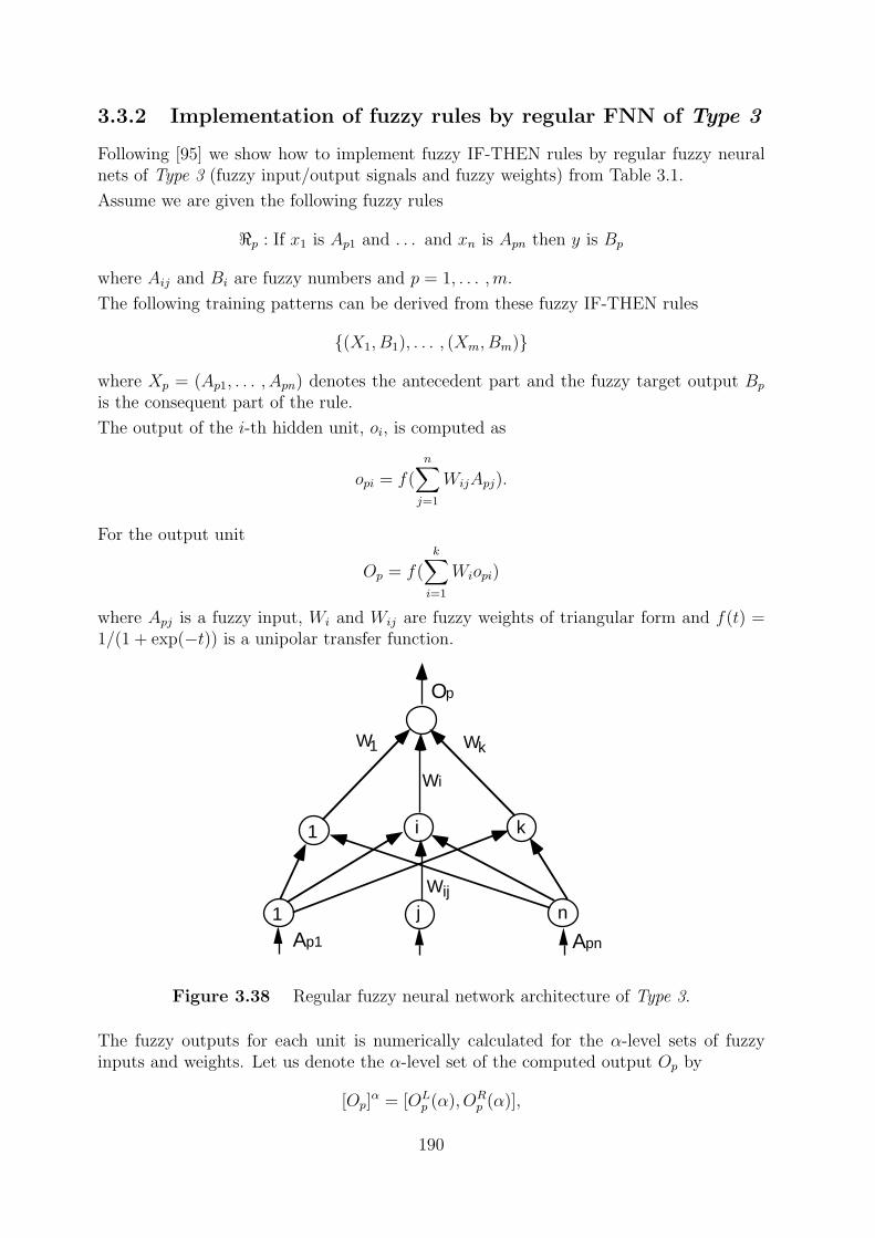
W
Wi
Οp
WW
Ap1 Apn
1 i k
1 j n
k1
ij
3.3.2 Implementation of fuzzy rules by regular FNN of Type 3
Following [95] we show how to implement fuzzy IF-THEN rules by regular fuzzy neuralnets of Type 3 (fuzzy input/output signals and fuzzy weights) from Table 3.1.
Assume we are given the following fuzzy rules
<p : If x1 is Ap1 and . . . and xn is Apn then y is Bp
where Aij and Bi are fuzzy numbers and p = 1, . . . ,m.
The following training patterns can be derived from these fuzzy IF-THEN rules
{(X1, B1), . . . , (Xm, Bm)}
where Xp = (Ap1, . . . , Apn) denotes the antecedent part and the fuzzy target output Bp
is the consequent part of the rule.
The output of the i-th hidden unit, oi, is computed as
opi = f(n∑j=1
WijApj).
For the output unit
Op = f(k∑i=1
Wiopi)
where Apj is a fuzzy input, Wi and Wij are fuzzy weights of triangular form and f(t) =1/(1 + exp(−t)) is a unipolar transfer function.
Figure 3.38 Regular fuzzy neural network architecture of Type 3.
The fuzzy outputs for each unit is numerically calculated for the α-level sets of fuzzyinputs and weights. Let us denote the α-level set of the computed output Op by
[Op]α = [OL
p (α), ORp (α)],
190
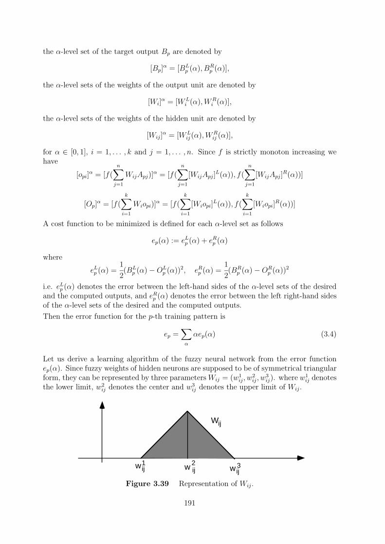
Wij
wij1 w ij
2wij
3
the α-level set of the target output Bp are denoted by
[Bp]α = [BL
p (α), BRp (α)],
the α-level sets of the weights of the output unit are denoted by
[Wi]α = [WL
i (α),WRi (α)],
the α-level sets of the weights of the hidden unit are denoted by
[Wij]α = [WL
ij (α),WRij (α)],
for α ∈ [0, 1], i = 1, . . . , k and j = 1, . . . , n. Since f is strictly monoton increasing wehave
[opi]α = [f(
n∑j=1
WijApj)]α = [f(
n∑j=1
[WijApj]L(α)), f(
n∑j=1
[WijApj]R(α))]
[Op]α = [f(
k∑i=1
Wiopi)]α = [f(
k∑i=1
[Wiopi]L(α)), f(
k∑i=1
[Wiopi]R(α))]
A cost function to be minimized is defined for each α-level set as follows
ep(α) := eLp (α) + eRp (α)
where
eLp (α) =1
2(BL
p (α)−OLp (α))2, eRp (α) =
1
2(BR
p (α)−ORp (α))2
i.e. eLp (α) denotes the error between the left-hand sides of the α-level sets of the desiredand the computed outputs, and eRp (α) denotes the error between the left right-hand sidesof the α-level sets of the desired and the computed outputs.
Then the error function for the p-th training pattern is
ep =∑α
αep(α) (3.4)
Let us derive a learning algorithm of the fuzzy neural network from the error functionep(α). Since fuzzy weights of hidden neurons are supposed to be of symmetrical triangularform, they can be represented by three parameters Wij = (w1
ij, w2ij, w
3ij). where w1
ij denotesthe lower limit, w2
ij denotes the center and w3ij denotes the upper limit of Wij.
Figure 3.39 Representation of Wij.
191
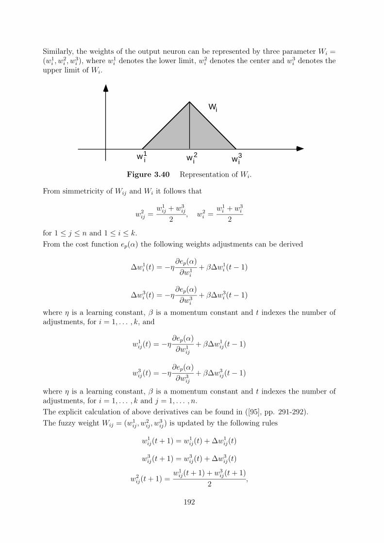
Wi
w i1 wi
2 wi3
Similarly, the weights of the output neuron can be represented by three parameter Wi =(w1
i , w2i , w
3i ), where w1
i denotes the lower limit, w2i denotes the center and w3
i denotes theupper limit of Wi.
Figure 3.40 Representation of Wi.
From simmetricity of Wij and Wi it follows that
w2ij =
w1ij + w3
ij
2, w2
i =w1i + w3
i
2
for 1 ≤ j ≤ n and 1 ≤ i ≤ k.
From the cost function ep(α) the following weights adjustments can be derived
∆w1i (t) = −η
∂ep(α)
∂w1i
+ β∆w1i (t− 1)
∆w3i (t) = −η
∂ep(α)
∂w3i
+ β∆w3i (t− 1)
where η is a learning constant, β is a momentum constant and t indexes the number ofadjustments, for i = 1, . . . , k, and
w1ij(t) = −η
∂ep(α)
∂w1ij
+ β∆w1ij(t− 1)
w3ij(t) = −η
∂ep(α)
∂w3ij
+ β∆w3ij(t− 1)
where η is a learning constant, β is a momentum constant and t indexes the number ofadjustments, for i = 1, . . . , k and j = 1, . . . , n.
The explicit calculation of above derivatives can be found in ([95], pp. 291-292).
The fuzzy weight Wij = (w1ij, w
2ij, w
3ij) is updated by the following rules
w1ij(t+ 1) = w1
ij(t) + ∆w1ij(t)
w3ij(t+ 1) = w3
ij(t) + ∆w3ij(t)
w2ij(t+ 1) =
w1ij(t+ 1) + w3
ij(t+ 1)
2,
192
for i = 1, . . . , k and j = 1, . . . , n. The fuzzy weight Wi = (w1i , w
2i , w
3i ) is updated in a
similar manner, i.e.w1i (t+ 1) = w1
i (t) + ∆w1i (t)
w3i (t+ 1) = w3
i (t) + ∆w3i (t)
w2i (t+ 1) =
w1i (t+ 1) + w3
i (t+ 1)
2,
for i = 1, . . . , k.
After the adjustment of Wi it can occur that its lower limit may become larger than itsupper limit. In this case, we use the following simple heuristics
w1i (t+ 1) := min{w1
i (t+ 1), w3i (t+ 1)}
w3i (t+ 1) := max{w1
i (t+ 1), w3i (t+ 1)}.
We employ the same heuristics for Wij.
w1ij(t+ 1) := min{w1
ij(t+ 1), w3ij(t+ 1)}
w3ij(t+ 1) := max{w1
ij(t+ 1), w3ij(t+ 1)}.
Let us assume that m input-output pairs
{(X1, B1), . . . , (Xm, Bm)}
where Xp = (Ap1, . . . , Apn), are given as training data.
We also assume that M values of α-level sets are used for the learning of the fuzzy neuralnetwork.
Summary 3.3.1 In this case, the learning algorithm can be summarized as follows:
• Step 1 Fuzzy weights are initialized at small random values, the running error Eis set to 0 and Emax > 0 is chosen
• Step 2 Repeat Step 3 for α = α1, α2, . . . , αM .
• Step 3 Repeat the following procedures for p = 1, 2, . . . ,m. Propagate Xp throughthe network and calculate the α-level set of the fuzzy output vector Op. Adjust thefuzzy weights using the error function ep(α).
• Step 4 Cumulative cycle error is computed by adding the present error to E.
• Step 5 The training cycle is completed. For E < Emax terminate the trainingsession. If E > Emax then E is set to 0 and we initiate a new training cycle bygoing back to Step 2.
193
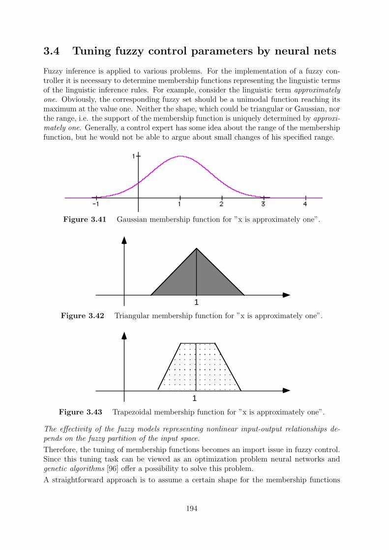
1
1
3.4 Tuning fuzzy control parameters by neural nets
Fuzzy inference is applied to various problems. For the implementation of a fuzzy con-troller it is necessary to determine membership functions representing the linguistic termsof the linguistic inference rules. For example, consider the linguistic term approximatelyone. Obviously, the corresponding fuzzy set should be a unimodal function reaching itsmaximum at the value one. Neither the shape, which could be triangular or Gaussian, northe range, i.e. the support of the membership function is uniquely determined by approxi-mately one. Generally, a control expert has some idea about the range of the membershipfunction, but he would not be able to argue about small changes of his specified range.
Figure 3.41 Gaussian membership function for ”x is approximately one”.
Figure 3.42 Triangular membership function for ”x is approximately one”.
Figure 3.43 Trapezoidal membership function for ”x is approximately one”.
The effectivity of the fuzzy models representing nonlinear input-output relationships de-pends on the fuzzy partition of the input space.
Therefore, the tuning of membership functions becomes an import issue in fuzzy control.Since this tuning task can be viewed as an optimization problem neural networks andgenetic algorithms [96] offer a possibility to solve this problem.
A straightforward approach is to assume a certain shape for the membership functions
194
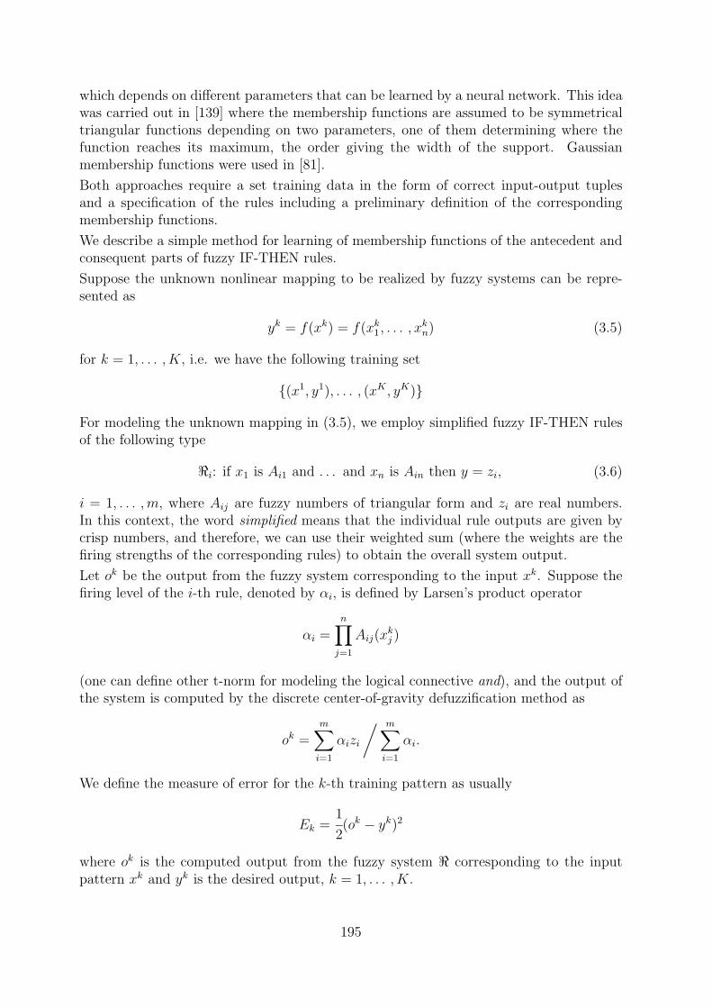
which depends on different parameters that can be learned by a neural network. This ideawas carried out in [139] where the membership functions are assumed to be symmetricaltriangular functions depending on two parameters, one of them determining where thefunction reaches its maximum, the order giving the width of the support. Gaussianmembership functions were used in [81].
Both approaches require a set training data in the form of correct input-output tuplesand a specification of the rules including a preliminary definition of the correspondingmembership functions.
We describe a simple method for learning of membership functions of the antecedent andconsequent parts of fuzzy IF-THEN rules.
Suppose the unknown nonlinear mapping to be realized by fuzzy systems can be repre-sented as
yk = f(xk) = f(xk1, . . . , xkn) (3.5)
for k = 1, . . . , K, i.e. we have the following training set
{(x1, y1), . . . , (xK , yK)}
For modeling the unknown mapping in (3.5), we employ simplified fuzzy IF-THEN rulesof the following type
<i: if x1 is Ai1 and . . . and xn is Ain then y = zi, (3.6)
i = 1, . . . ,m, where Aij are fuzzy numbers of triangular form and zi are real numbers.In this context, the word simplified means that the individual rule outputs are given bycrisp numbers, and therefore, we can use their weighted sum (where the weights are thefiring strengths of the corresponding rules) to obtain the overall system output.
Let ok be the output from the fuzzy system corresponding to the input xk. Suppose thefiring level of the i-th rule, denoted by αi, is defined by Larsen’s product operator
αi =n∏j=1
Aij(xkj )
(one can define other t-norm for modeling the logical connective and), and the output ofthe system is computed by the discrete center-of-gravity defuzzification method as
ok =m∑i=1
αizi
/ m∑i=1
αi.
We define the measure of error for the k-th training pattern as usually
Ek =1
2(ok − yk)2
where ok is the computed output from the fuzzy system < corresponding to the inputpattern xk and yk is the desired output, k = 1, . . . , K.
195
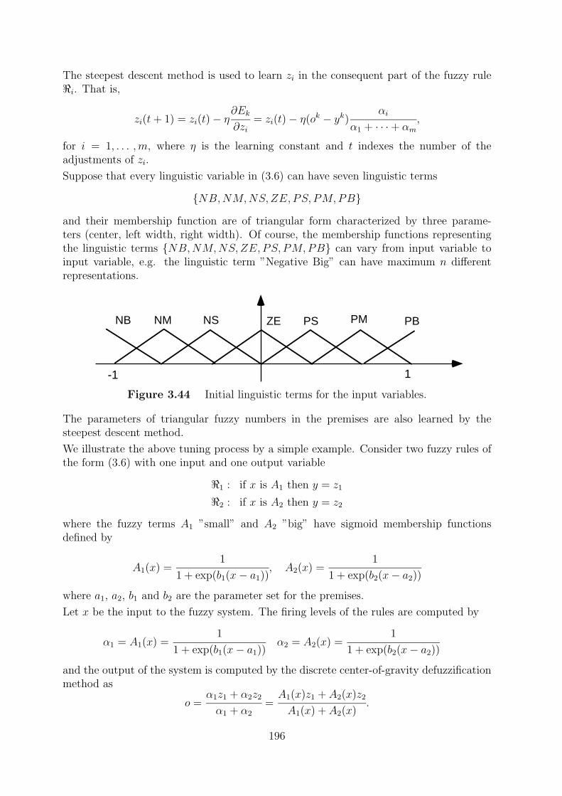
NB PBPMPSZENSNM
-1 1
The steepest descent method is used to learn zi in the consequent part of the fuzzy rule<i. That is,
zi(t+ 1) = zi(t)− η∂Ek
∂zi= zi(t)− η(ok − yk)
αi
α1 + · · ·+ αm,
for i = 1, . . . ,m, where η is the learning constant and t indexes the number of theadjustments of zi.
Suppose that every linguistic variable in (3.6) can have seven linguistic terms
{NB,NM,NS,ZE, PS, PM,PB}
and their membership function are of triangular form characterized by three parame-ters (center, left width, right width). Of course, the membership functions representingthe linguistic terms {NB,NM,NS,ZE, PS, PM,PB} can vary from input variable toinput variable, e.g. the linguistic term ”Negative Big” can have maximum n differentrepresentations.
Figure 3.44 Initial linguistic terms for the input variables.
The parameters of triangular fuzzy numbers in the premises are also learned by thesteepest descent method.
We illustrate the above tuning process by a simple example. Consider two fuzzy rules ofthe form (3.6) with one input and one output variable
<1 : if x is A1 then y = z1
<2 : if x is A2 then y = z2
where the fuzzy terms A1 ”small” and A2 ”big” have sigmoid membership functionsdefined by
A1(x) =1
1 + exp(b1(x− a1)), A2(x) =
1
1 + exp(b2(x− a2))
where a1, a2, b1 and b2 are the parameter set for the premises.
Let x be the input to the fuzzy system. The firing levels of the rules are computed by
α1 = A1(x) =1
1 + exp(b1(x− a1))α2 = A2(x) =
1
1 + exp(b2(x− a2))
and the output of the system is computed by the discrete center-of-gravity defuzzificationmethod as
o =α1z1 + α2z2
α1 + α2
=A1(x)z1 + A2(x)z2
A1(x) + A2(x).
196
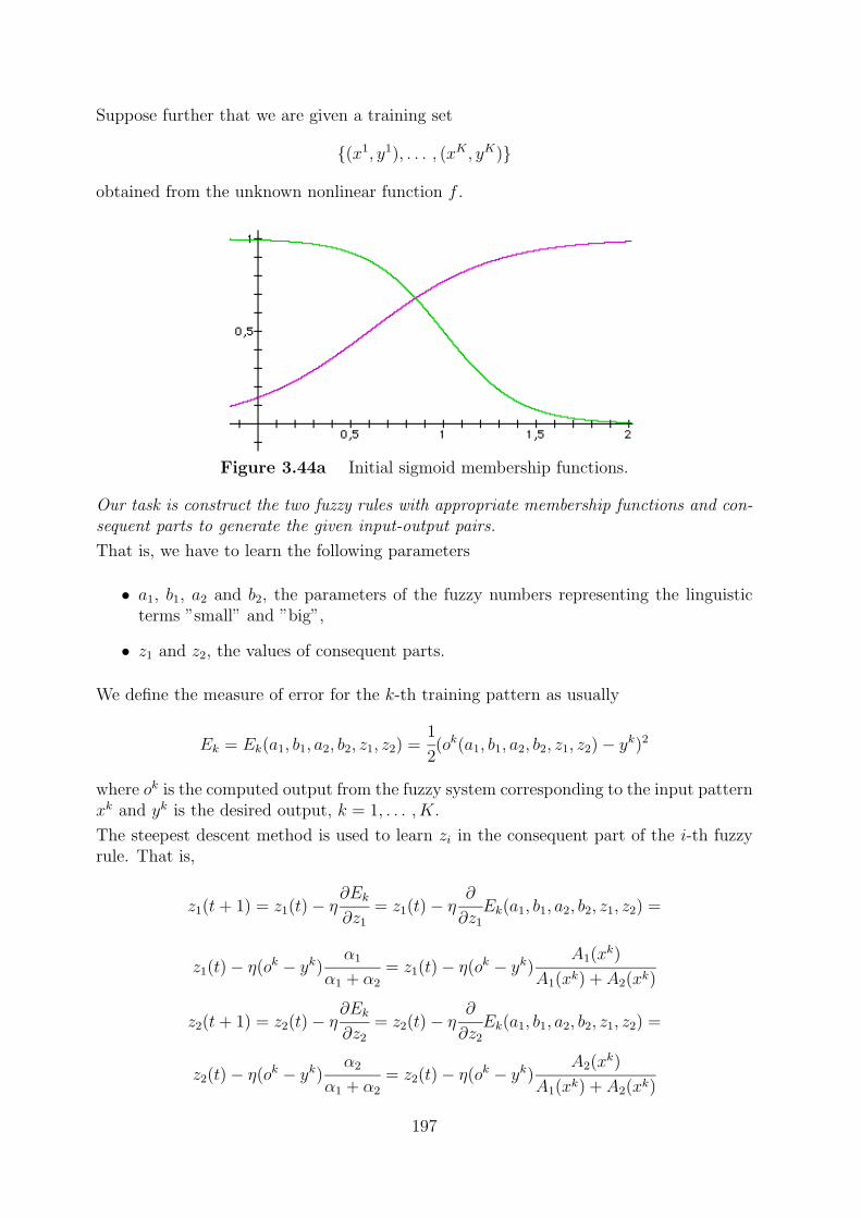
Suppose further that we are given a training set
{(x1, y1), . . . , (xK , yK)}
obtained from the unknown nonlinear function f .
Figure 3.44a Initial sigmoid membership functions.
Our task is construct the two fuzzy rules with appropriate membership functions and con-sequent parts to generate the given input-output pairs.
That is, we have to learn the following parameters
• a1, b1, a2 and b2, the parameters of the fuzzy numbers representing the linguisticterms ”small” and ”big”,
• z1 and z2, the values of consequent parts.
We define the measure of error for the k-th training pattern as usually
Ek = Ek(a1, b1, a2, b2, z1, z2) =1
2(ok(a1, b1, a2, b2, z1, z2)− yk)2
where ok is the computed output from the fuzzy system corresponding to the input patternxk and yk is the desired output, k = 1, . . . , K.
The steepest descent method is used to learn zi in the consequent part of the i-th fuzzyrule. That is,
z1(t+ 1) = z1(t)− η∂Ek
∂z1
= z1(t)− η∂
∂z1
Ek(a1, b1, a2, b2, z1, z2) =
z1(t)− η(ok − yk)α1
α1 + α2
= z1(t)− η(ok − yk)A1(xk)
A1(xk) + A2(xk)
z2(t+ 1) = z2(t)− η∂Ek
∂z2
= z2(t)− η∂
∂z2
Ek(a1, b1, a2, b2, z1, z2) =
z2(t)− η(ok − yk)α2
α1 + α2
= z2(t)− η(ok − yk)A2(xk)
A1(xk) + A2(xk)
197
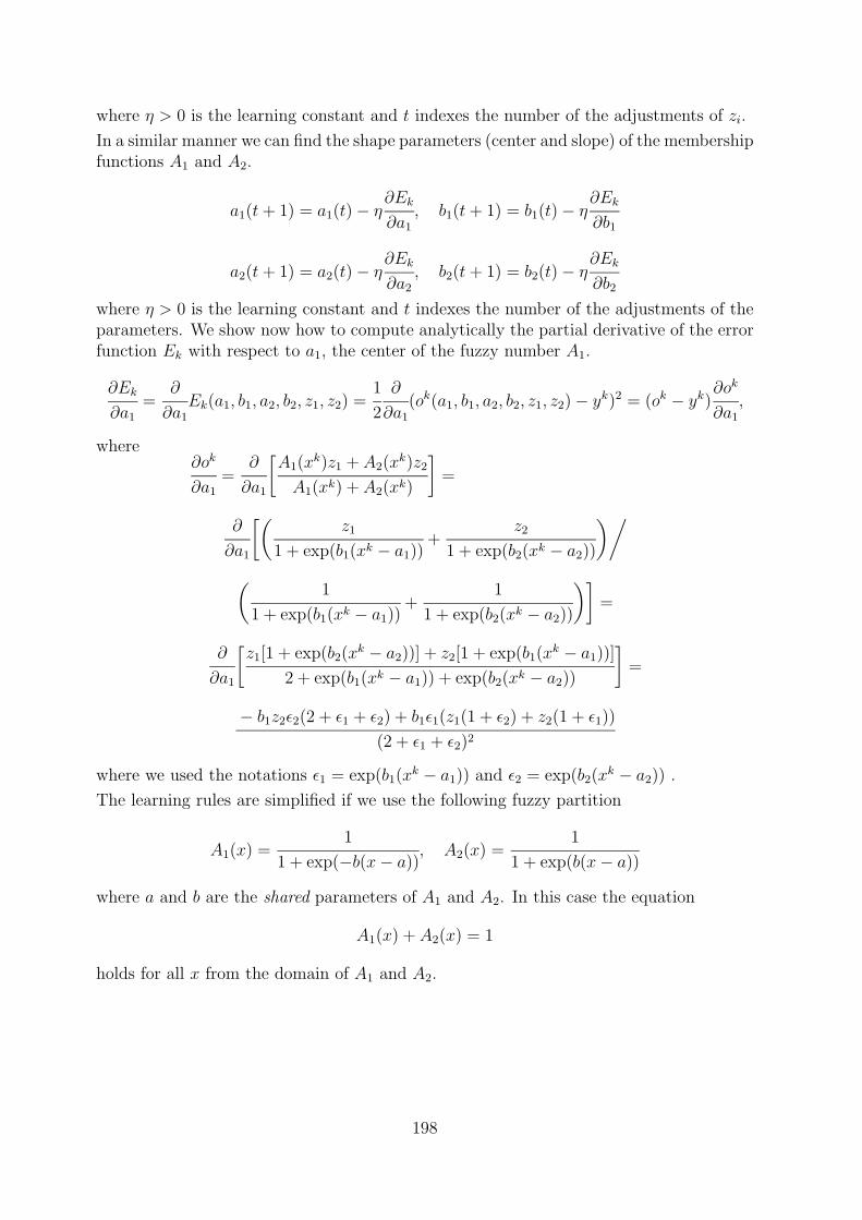
where η > 0 is the learning constant and t indexes the number of the adjustments of zi.
In a similar manner we can find the shape parameters (center and slope) of the membershipfunctions A1 and A2.
a1(t+ 1) = a1(t)− η∂Ek
∂a1
, b1(t+ 1) = b1(t)− η∂Ek
∂b1
a2(t+ 1) = a2(t)− η∂Ek
∂a2
, b2(t+ 1) = b2(t)− η∂Ek
∂b2
where η > 0 is the learning constant and t indexes the number of the adjustments of theparameters. We show now how to compute analytically the partial derivative of the errorfunction Ek with respect to a1, the center of the fuzzy number A1.
∂Ek
∂a1
=∂
∂a1
Ek(a1, b1, a2, b2, z1, z2) =1
2
∂
∂a1
(ok(a1, b1, a2, b2, z1, z2)− yk)2 = (ok − yk)∂ok
∂a1
,
where∂ok
∂a1
=∂
∂a1
[A1(xk)z1 + A2(xk)z2
A1(xk) + A2(xk)
]=
∂
∂a1
[(z1
1 + exp(b1(xk − a1))+
z2
1 + exp(b2(xk − a2))
)/(
1
1 + exp(b1(xk − a1))+
1
1 + exp(b2(xk − a2))
)]=
∂
∂a1
[z1[1 + exp(b2(xk − a2))] + z2[1 + exp(b1(xk − a1))]
2 + exp(b1(xk − a1)) + exp(b2(xk − a2))
]=
− b1z2ε2(2 + ε1 + ε2) + b1ε1(z1(1 + ε2) + z2(1 + ε1))
(2 + ε1 + ε2)2
where we used the notations ε1 = exp(b1(xk − a1)) and ε2 = exp(b2(xk − a2)) .
The learning rules are simplified if we use the following fuzzy partition
A1(x) =1
1 + exp(−b(x− a)), A2(x) =
1
1 + exp(b(x− a))
where a and b are the shared parameters of A1 and A2. In this case the equation
A1(x) + A2(x) = 1
holds for all x from the domain of A1 and A2.
198
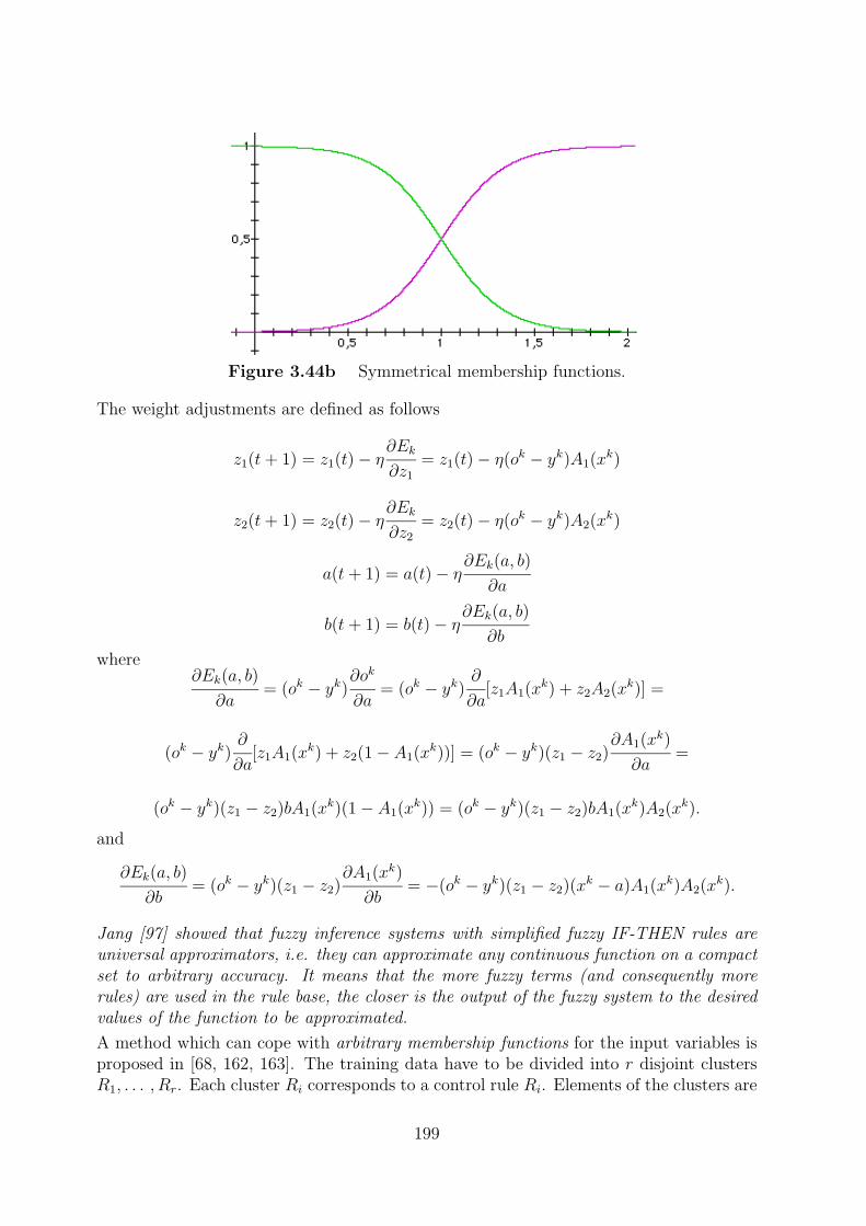
Figure 3.44b Symmetrical membership functions.
The weight adjustments are defined as follows
z1(t+ 1) = z1(t)− η∂Ek
∂z1
= z1(t)− η(ok − yk)A1(xk)
z2(t+ 1) = z2(t)− η∂Ek
∂z2
= z2(t)− η(ok − yk)A2(xk)
a(t+ 1) = a(t)− η∂Ek(a, b)
∂a
b(t+ 1) = b(t)− η∂Ek(a, b)
∂b
where∂Ek(a, b)
∂a= (ok − yk)
∂ok
∂a= (ok − yk)
∂
∂a[z1A1(xk) + z2A2(xk)] =
(ok − yk)∂
∂a[z1A1(xk) + z2(1− A1(xk))] = (ok − yk)(z1 − z2)
∂A1(xk)
∂a=
(ok − yk)(z1 − z2)bA1(xk)(1− A1(xk)) = (ok − yk)(z1 − z2)bA1(xk)A2(xk).
and
∂Ek(a, b)
∂b= (ok − yk)(z1 − z2)
∂A1(xk)
∂b= −(ok − yk)(z1 − z2)(xk − a)A1(xk)A2(xk).
Jang [97] showed that fuzzy inference systems with simplified fuzzy IF-THEN rules areuniversal approximators, i.e. they can approximate any continuous function on a compactset to arbitrary accuracy. It means that the more fuzzy terms (and consequently morerules) are used in the rule base, the closer is the output of the fuzzy system to the desiredvalues of the function to be approximated.
A method which can cope with arbitrary membership functions for the input variables isproposed in [68, 162, 163]. The training data have to be divided into r disjoint clustersR1, . . . , Rr. Each cluster Ri corresponds to a control rule Ri. Elements of the clusters are
199
tuples of input-output values of the form (x, y) where x can be a vector x = (x1, . . . , xn)of n input variables.
This means that the rules are not specified in terms of linguistic variables, but in the formof crisp input-output tuples.
A multilayer perceptron with n input units, some hidden layers, and r output units canbe used to learn these clusters. The input data for this learning task are the input vectorsof all clusters, i.e. the set
{x | ∃i ∃y : (x, y) ∈ Ri}.The target output tui(x) for input x at output unit ui is defined as
tui(x) =
{1 if there exists y such that (x, y) ∈ Ri
0 otherwise
After the network has learned its weights, arbitrary values for x can be taken as inputs.Then the output at output unit ui can be interpreted as the degree to which x matchesthe antecedent of rule Ri, i.e. the function
x→ oui
is the membership function for the fuzzy set representing the linguistic term on the left-hand side of rule Ri.
In case of a Mamdani type fuzzy controller the same technique can be applied to theoutput variable, resulting in a neural network which determines the fuzzy sets for theright-hand sides of the rules.
For Sugeno type fuzzy controller, where each rule yields a crisp output value togetherwith a number, specifying the matching degree for the antecedent of the rule, anothertechnique can be applied. For each rule Ri a neural network is trained with the input-output tuples of the set Ri. Thus these r neural networks determine the crisp outputvalues for the rules Ri, . . . , Rr.
These neural networks can also be used to eliminate unnecessary input variables in theinput vector x for the rules R1, . . . , Rr by neglecting one input variable in one of the rulesand comparing the control result with the one, when the variable is not neglected. If theperformance of the controller is not influenced by neglecting input variable xj in rule Ri,xj is unnecessary for Ri and can be left out.
ANFIS (Adaptive Neural Fuzzy Inference Systems) [97] is a great example of an archi-tecture for tuning fuzzy system parameters from input/output pairs of data. The fuzzyinference process is implemented as a generalized neural network, which is then tuned bygradient descent techniques. It is capable of tuning antecedent parameters as well as con-sequent parameters of fuzzy rules which use a softened trapezoidal membership function.It has been applied to a variety of problems, including chaotic time series prediction andthe IRIS cluster learning problem.
These tuning methods has a weak point, because the convergence of tuning depends on theinitial condition. Ishigami, Fukuda, Shibata and Arai [96] present a hybrid auto-tuningmethod of fuzzy inference using genetic algorithms and the generalized delta learning rule,which guarantees the optimal structure of the fuzzy model.
200
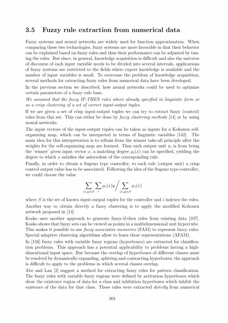
3.5 Fuzzy rule extraction from numerical data
Fuzzy systems and neural networks are widely used for function approximation. Whencomparing these two technologies, fuzzy systems are more favorable in that their behaviorcan be explained based on fuzzy rules and thus their performance can be adjusted by tun-ing the rules. But since, in general, knowledge acquisition is difficult and also the universeof discourse of each input variable needs to be divided into several intervals, applicationsof fuzzy systems are restricted to the fields where expert knowledge is available and thenumber of input variables is small. To overcome the problem of knowledge acquisition,several methods for extracting fuzzy rules from numerical data have been developed.
In the previous section we described, how neural networks could be used to optimizecertain parameters of a fuzzy rule base.
We assumed that the fuzzy IF-THEN rules where already specified in linguistic form oras a crisp clustering of a set of correct input-output tuples.
If we are given a set of crisp input-output tuples we can try to extract fuzzy (control)rules from this set. This can either be done by fuzzy clustering methods [14] or by usingneural networks.
The input vectors of the input-output tuples can be taken as inputs for a Kohonen self-organizing map, which can be interpreted in terms of linguistic variables [142]. Themain idea for this interpretation is to refrain from the winner take-all principle after theweights for the self-organizing map are learned. Thus each output unit ui is from beingthe ’winner’ given input vector x, a matching degree µi(x) can be specified, yielding thedegree to which x satisfies the antecedent of the corresponding rule.
Finally, in order to obtain a Sugeno type controller, to each rule (output unit) a crispcontrol output value has to be associated. Following the idea of the Sugeno type controller,we could choose the value ∑
(x,y)∈S
∑i
µi(x)y
/ ∑(x,y)∈S
µi(x)
where S is the set of known input-output tuples for the controller and i indexes the rules.
Another way to obtain directly a fuzzy clustering is to apply the modified Kohonennetwork proposed in [13].
Kosko uses another approach to generate fuzzy-if-then rules from existing data [107].Kosko shows that fuzzy sets can be viewed as points in a multidimensional unit hypercube.This makes it possible to use fuzzy associative memories (FAM) to represent fuzzy rules.Special adaptive clustering algorithms allow to learn these representations (AFAM).
In [156] fuzzy rules with variable fuzzy regions (hyperboxes) are extracted for classifica-tion problems. This approach has a potential applicability to problems having a high-dimentional input space. But because the overlap of hyperboxes of different classes mustbe resolved by dynamically expanding, splitting and contracting hyperboxes, the approachis difficult to apply to the problems in which several classes overlap.
Abe and Lan [2] suggest a method for extracting fuzzy rules for pattern classification.The fuzzy rules with variable fuzzy regions were defined by activation hyperboxes whichshow the existence region of data for a class and inhibition hyperboxes which inhibit theexistence of the data for that class. These rules were extracted directly from numerical
201
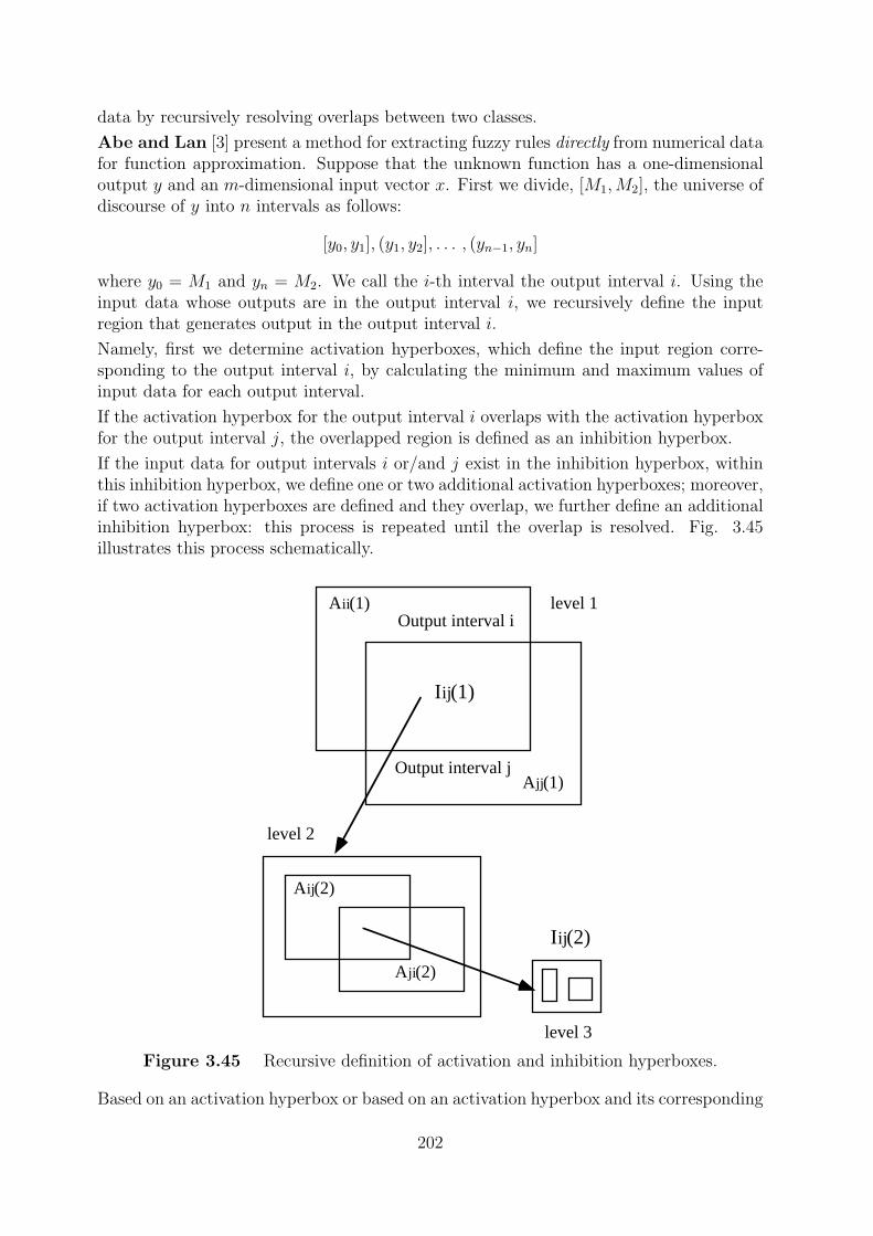
Output interval ilevel 1
level 2
level 3
Aii(1)
Ajj(1)Output interval j
I ij(1)
Aij(2)
Aji(2)
I ij(2)
data by recursively resolving overlaps between two classes.
Abe and Lan [3] present a method for extracting fuzzy rules directly from numerical datafor function approximation. Suppose that the unknown function has a one-dimensionaloutput y and an m-dimensional input vector x. First we divide, [M1,M2], the universe ofdiscourse of y into n intervals as follows:
[y0, y1], (y1, y2], . . . , (yn−1, yn]
where y0 = M1 and yn = M2. We call the i-th interval the output interval i. Using theinput data whose outputs are in the output interval i, we recursively define the inputregion that generates output in the output interval i.
Namely, first we determine activation hyperboxes, which define the input region corre-sponding to the output interval i, by calculating the minimum and maximum values ofinput data for each output interval.
If the activation hyperbox for the output interval i overlaps with the activation hyperboxfor the output interval j, the overlapped region is defined as an inhibition hyperbox.
If the input data for output intervals i or/and j exist in the inhibition hyperbox, withinthis inhibition hyperbox, we define one or two additional activation hyperboxes; moreover,if two activation hyperboxes are defined and they overlap, we further define an additionalinhibition hyperbox: this process is repeated until the overlap is resolved. Fig. 3.45illustrates this process schematically.
Figure 3.45 Recursive definition of activation and inhibition hyperboxes.
Based on an activation hyperbox or based on an activation hyperbox and its corresponding
202
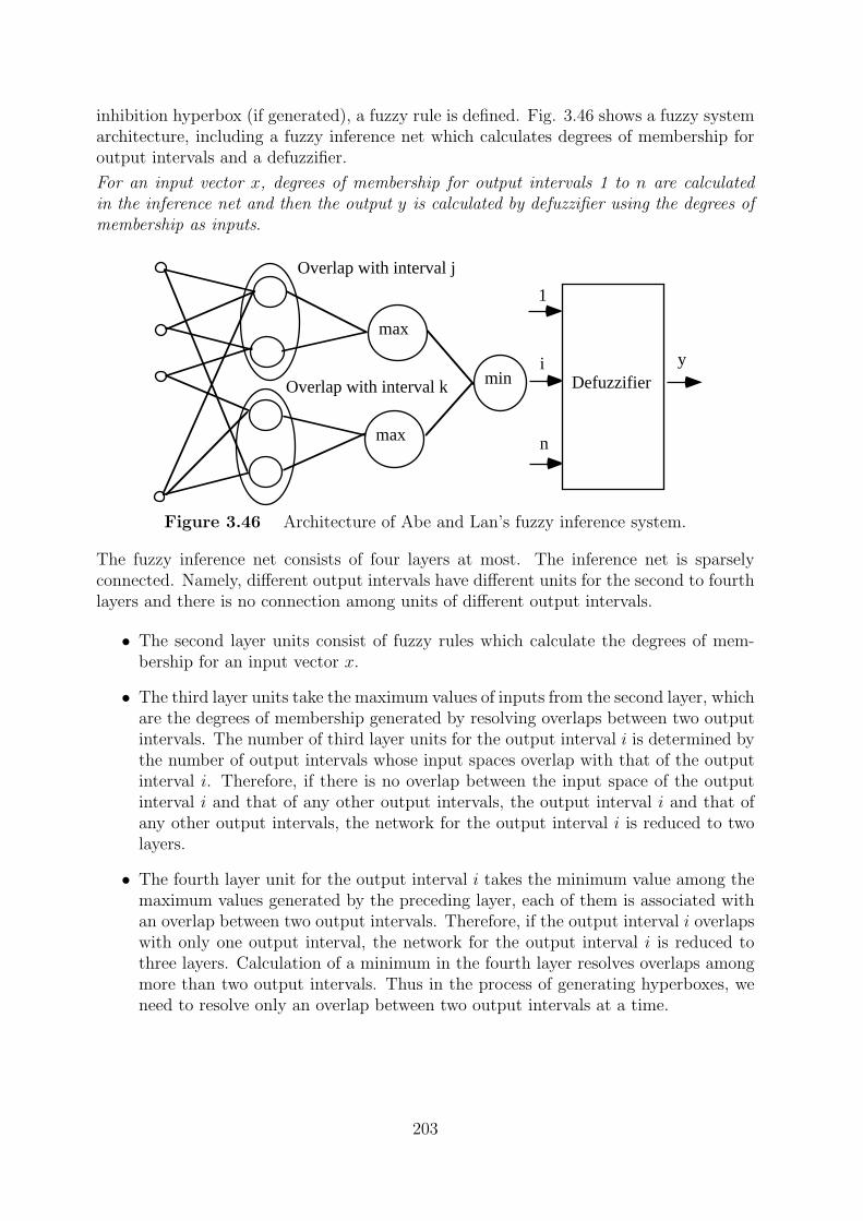
max
max
miny
1
i
n
Overlap with interval j
Overlap with interval k Defuzzifier
inhibition hyperbox (if generated), a fuzzy rule is defined. Fig. 3.46 shows a fuzzy systemarchitecture, including a fuzzy inference net which calculates degrees of membership foroutput intervals and a defuzzifier.
For an input vector x, degrees of membership for output intervals 1 to n are calculatedin the inference net and then the output y is calculated by defuzzifier using the degrees ofmembership as inputs.
Figure 3.46 Architecture of Abe and Lan’s fuzzy inference system.
The fuzzy inference net consists of four layers at most. The inference net is sparselyconnected. Namely, different output intervals have different units for the second to fourthlayers and there is no connection among units of different output intervals.
• The second layer units consist of fuzzy rules which calculate the degrees of mem-bership for an input vector x.
• The third layer units take the maximum values of inputs from the second layer, whichare the degrees of membership generated by resolving overlaps between two outputintervals. The number of third layer units for the output interval i is determined bythe number of output intervals whose input spaces overlap with that of the outputinterval i. Therefore, if there is no overlap between the input space of the outputinterval i and that of any other output intervals, the output interval i and that ofany other output intervals, the network for the output interval i is reduced to twolayers.
• The fourth layer unit for the output interval i takes the minimum value among themaximum values generated by the preceding layer, each of them is associated withan overlap between two output intervals. Therefore, if the output interval i overlapswith only one output interval, the network for the output interval i is reduced tothree layers. Calculation of a minimum in the fourth layer resolves overlaps amongmore than two output intervals. Thus in the process of generating hyperboxes, weneed to resolve only an overlap between two output intervals at a time.
203
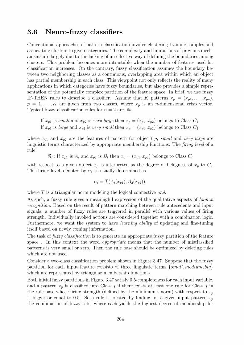
3.6 Neuro-fuzzy classifiers
Conventional approaches of pattern classification involve clustering training samples andassociating clusters to given categories. The complexity and limitations of previous mech-anisms are largely due to the lacking of an effective way of defining the boundaries amongclusters. This problem becomes more intractable when the number of features used forclassification increases. On the contrary, fuzzy classification assumes the boundary be-tween two neighboring classes as a continuous, overlapping area within which an objecthas partial membership in each class. This viewpoint not only reflects the reality of manyapplications in which categories have fuzzy boundaries, but also provides a simple repre-sentation of the potentially complex partition of the feature space. In brief, we use fuzzyIF-THEN rules to describe a classifier. Assume that K patterns xp = (xp1, . . . , xpn),p = 1, . . . , K are given from two classes, where xp is an n-dimensional crisp vector.Typical fuzzy classification rules for n = 2 are like
If xp1 is small and xp2 is very large then xp = (xp1, xp2) belongs to Class C1
If xp1 is large and xp2 is very small then xp = (xp1, xp2) belongs to Class C2
where xp1 and xp2 are the features of pattern (or object) p, small and very large arelinguistic terms characterized by appropriate membership functions. The firing level of arule
<i : If xp1 is Ai and xp2 is Bi then xp = (xp1, xp2) belongs to Class Ci
with respect to a given object xp is interpreted as the degree of belogness of xp to Ci.This firing level, denoted by αi, is usually determined as
αi = T (Ai(xp1), A2(xp2)),
where T is a triangular norm modeling the logical connective and.
As such, a fuzzy rule gives a meaningful expression of the qualitative aspects of humanrecognition. Based on the result of pattern matching between rule antecedents and inputsignals, a number of fuzzy rules are triggered in parallel with various values of firingstrength. Individually invoked actions are considered together with a combination logic.Furthermore, we want the system to have learning ability of updating and fine-tuningitself based on newly coming information.
The task of fuzzy classification is to generate an appropriate fuzzy partition of the featurespace . In this context the word appropriate means that the number of misclassifiedpatterns is very small or zero. Then the rule base should be optimized by deleting ruleswhich are not used.
Consider a two-class classification problem shown in Figure 3.47. Suppose that the fuzzypartition for each input feature consists of three linguistic terms {small,medium, big}which are represented by triangular membership functions.
Both initial fuzzy partitions in Figure 3.47 satisfy 0.5-completeness for each input variable,and a pattern xp is classified into Class j if there exists at least one rule for Class j inthe rule base whose firing strength (defined by the minimum t-norm) with respect to xpis bigger or equal to 0.5. So a rule is created by finding for a given input pattern xpthe combination of fuzzy sets, where each yields the highest degree of membership for
204
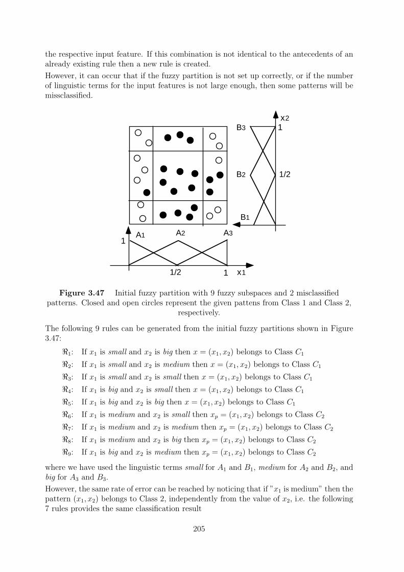
A1 A2 A3
B1
B2
B3
1
1
1
1/2
1/2
x1
x2
the respective input feature. If this combination is not identical to the antecedents of analready existing rule then a new rule is created.
However, it can occur that if the fuzzy partition is not set up correctly, or if the numberof linguistic terms for the input features is not large enough, then some patterns will bemissclassified.
Figure 3.47 Initial fuzzy partition with 9 fuzzy subspaces and 2 misclassifiedpatterns. Closed and open circles represent the given pattens from Class 1 and Class 2,
respectively.
The following 9 rules can be generated from the initial fuzzy partitions shown in Figure3.47:
<1: If x1 is small and x2 is big then x = (x1, x2) belongs to Class C1
<2: If x1 is small and x2 is medium then x = (x1, x2) belongs to Class C1
<3: If x1 is small and x2 is small then x = (x1, x2) belongs to Class C1
<4: If x1 is big and x2 is small then x = (x1, x2) belongs to Class C1
<5: If x1 is big and x2 is big then x = (x1, x2) belongs to Class C1
<6: If x1 is medium and x2 is small then xp = (x1, x2) belongs to Class C2
<7: If x1 is medium and x2 is medium then xp = (x1, x2) belongs to Class C2
<8: If x1 is medium and x2 is big then xp = (x1, x2) belongs to Class C2
<9: If x1 is big and x2 is medium then xp = (x1, x2) belongs to Class C2
where we have used the linguistic terms small for A1 and B1, medium for A2 and B2, andbig for A3 and B3.
However, the same rate of error can be reached by noticing that if ”x1 is medium” then thepattern (x1, x2) belongs to Class 2, independently from the value of x2, i.e. the following7 rules provides the same classification result
205
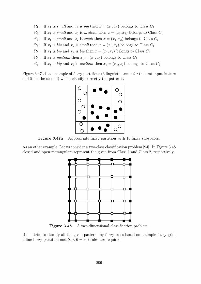
<1: If x1 is small and x2 is big then x = (x1, x2) belongs to Class C1
<2: If x1 is small and x2 is medium then x = (x1, x2) belongs to Class C1
<3: If x1 is small and x2 is small then x = (x1, x2) belongs to Class C1
<4: If x1 is big and x2 is small then x = (x1, x2) belongs to Class C1
<5: If x1 is big and x2 is big then x = (x1, x2) belongs to Class C1
<6: If x1 is medium then xp = (x1, x2) belongs to Class C2
<7: If x1 is big and x2 is medium then xp = (x1, x2) belongs to Class C2
Figure 3.47a is an example of fuzzy partitions (3 linguistic terms for the first input featureand 5 for the second) which classify correctly the patterns.
Figure 3.47a Appropriate fuzzy partition with 15 fuzzy subspaces.
As an other example, Let us consider a two-class classification problem [94]. In Figure 3.48closed and open rectangulars represent the given from Class 1 and Class 2, respectively.
Figure 3.48 A two-dimensional classification problem.
If one tries to classify all the given patterns by fuzzy rules based on a simple fuzzy grid,a fine fuzzy partition and (6× 6 = 36) rules are required.
206
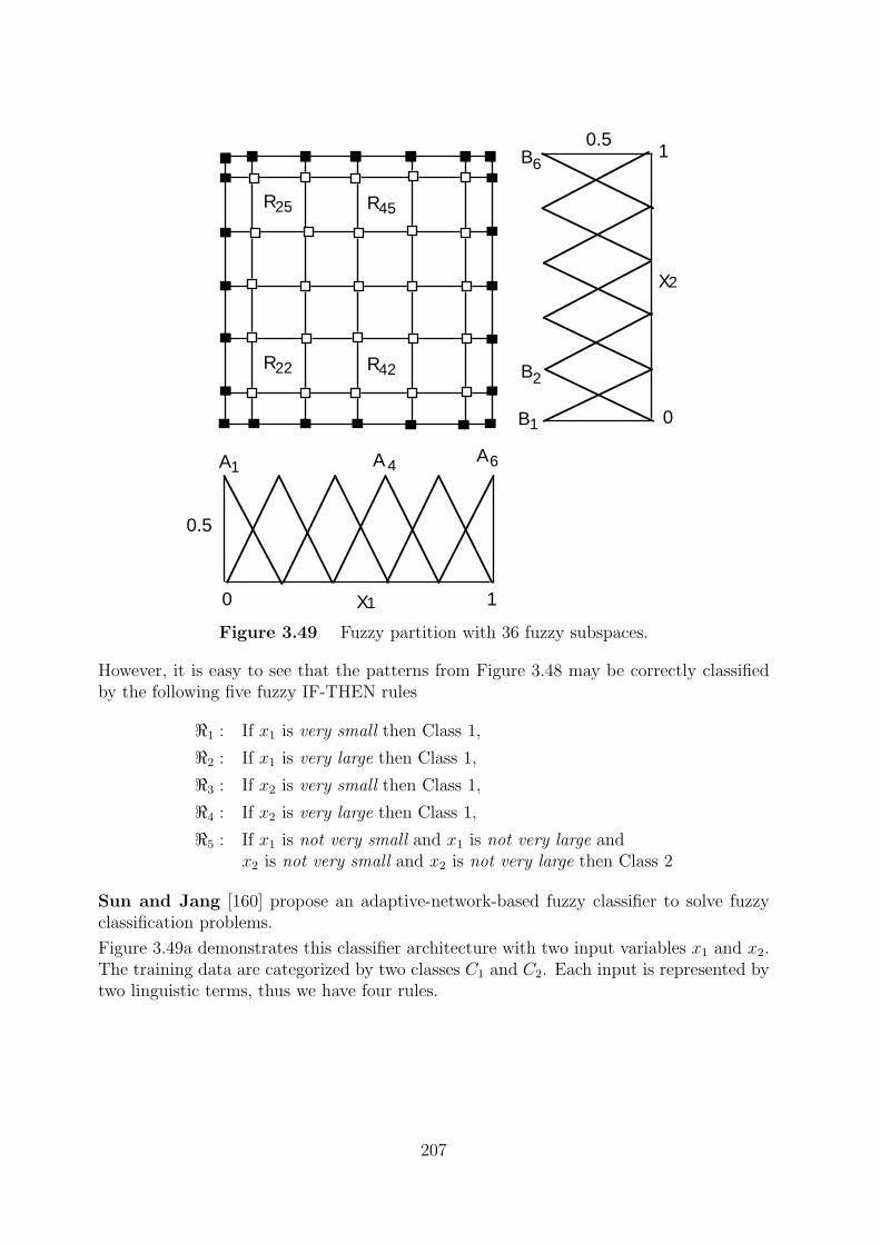
0 1X1
1
0
X2
0.5
0.5
R22 R42
R45R25
A 4A1A6
B
B
B1
2
6
Figure 3.49 Fuzzy partition with 36 fuzzy subspaces.
However, it is easy to see that the patterns from Figure 3.48 may be correctly classifiedby the following five fuzzy IF-THEN rules
<1 : If x1 is very small then Class 1,
<2 : If x1 is very large then Class 1,
<3 : If x2 is very small then Class 1,
<4 : If x2 is very large then Class 1,
<5 : If x1 is not very small and x1 is not very large andx2 is not very small and x2 is not very large then Class 2
Sun and Jang [160] propose an adaptive-network-based fuzzy classifier to solve fuzzyclassification problems.
Figure 3.49a demonstrates this classifier architecture with two input variables x1 and x2.The training data are categorized by two classes C1 and C2. Each input is represented bytwo linguistic terms, thus we have four rules.
207
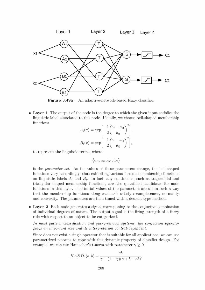
A1
A2
B1
B2
T
T
Layer 1 Layer 2 Layer 3 Layer 4
x1
x2
T
T
S
S
C1
C2
Figure 3.49a An adaptive-network-based fuzzy classifier.
• Layer 1 The output of the node is the degree to which the given input satisfies thelinguistic label associated to this node. Usually, we choose bell-shaped membershipfunctions
Ai(u) = exp
[−
1
2
(u− ai1bi1
)2],
Bi(v) = exp
[−
1
2
(v − ai2bi2
)2],
to represent the linguistic terms, where
{ai1, ai2, bi1, bi2}
is the parameter set. As the values of these parameters change, the bell-shapedfunctions vary accordingly, thus exhibiting various forms of membership functionson linguistic labels Ai and Bi. In fact, any continuous, such as trapezoidal andtriangular-shaped membership functions, are also quantified candidates for nodefunctions in this layer. The initial values of the parameters are set in such a waythat the membership functions along each axis satisfy ε-completeness, normalityand convexity. The parameters are then tuned with a descent-type method.
• Layer 2 Each node generates a signal corresponing to the conjuctive combinationof individual degrees of match. The output signal is the firing strength of a fuzzyrule with respect to an object to be categorized.
In most pattern classification and query-retrival systems, the conjuction operatorplays an important role and its interpretation context-dependent.
Since does not exist a single operator that is suitable for all applications, we can useparametrized t-norms to cope with this dynamic property of classifier design. Forexample, we can use Hamacher’s t-norm with parameter γ ≥ 0
HANDγ(a, b) =ab
γ + (1− γ)(a+ b− ab),
208
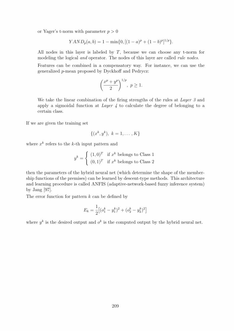
or Yager’s t-norm with parameter p > 0
Y ANDp(a, b) = 1−min{0, [(1− a)p + (1− b)p]1/p}.
All nodes in this layer is labeled by T , because we can choose any t-norm formodeling the logical and operator. The nodes of this layer are called rule nodes.
Features can be combined in a compensatory way. For instance, we can use thegeneralized p-mean proposed by Dyckhoff and Pedrycz:(
xp + yp
2
)1/p
, p ≥ 1.
We take the linear combination of the firing strengths of the rules at Layer 3 andapply a sigmoidal function at Layer 4 to calculate the degree of belonging to acertain class.
If we are given the training set
{(xk, yk), k = 1, . . . , K}
where xk refers to the k-th input pattern and
yk =
{(1, 0)T if xk belongs to Class 1
(0, 1)T if xk belongs to Class 2
then the parameters of the hybrid neural net (which determine the shape of the member-ship functions of the premises) can be learned by descent-type methods. This architectureand learning procedure is called ANFIS (adaptive-network-based fuzzy inference system)by Jang [97].
The error function for pattern k can be defined by
Ek =1
2
[(ok1 − yk1)2 + (ok2 − yk2)2
]where yk is the desired output and ok is the computed output by the hybrid neural net.
209
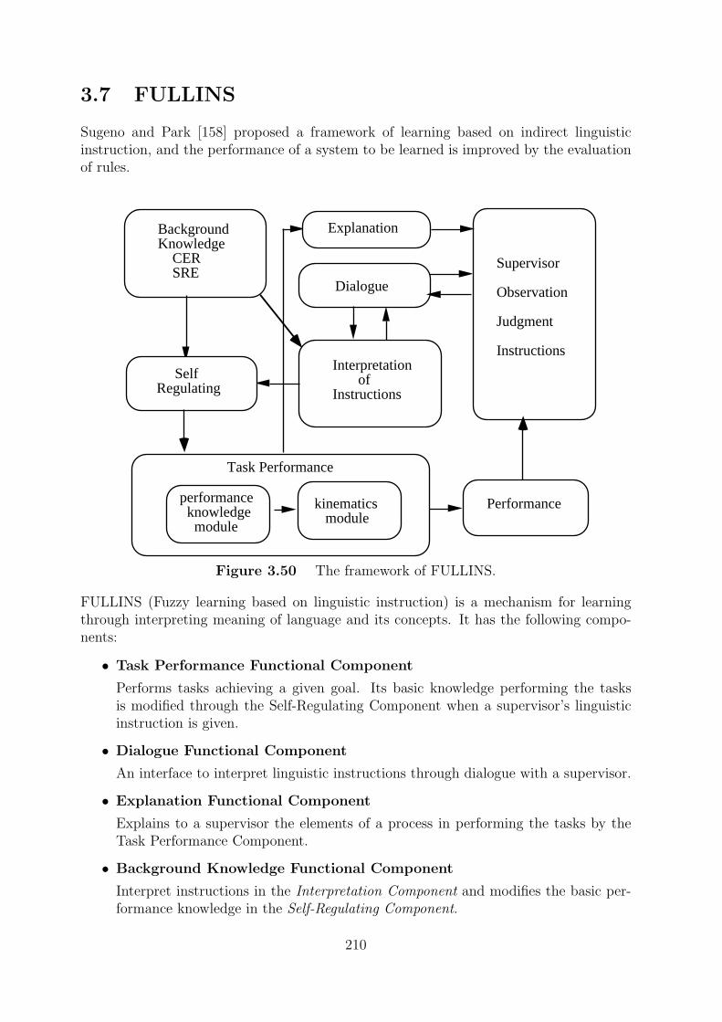
BackgroundKnowledge CER SRE
Interpretation ofInstructions
Dialogue
Performance
Supervisor Observation
Judgment
Instructions
SelfRegulating
Explanation
kinematics module
performance knowledge module
Task Performance
3.7 FULLINS
Sugeno and Park [158] proposed a framework of learning based on indirect linguisticinstruction, and the performance of a system to be learned is improved by the evaluationof rules.
Figure 3.50 The framework of FULLINS.
FULLINS (Fuzzy learning based on linguistic instruction) is a mechanism for learningthrough interpreting meaning of language and its concepts. It has the following compo-nents:
• Task Performance Functional Component
Performs tasks achieving a given goal. Its basic knowledge performing the tasksis modified through the Self-Regulating Component when a supervisor’s linguisticinstruction is given.
• Dialogue Functional Component
An interface to interpret linguistic instructions through dialogue with a supervisor.
• Explanation Functional Component
Explains to a supervisor the elements of a process in performing the tasks by theTask Performance Component.
• Background Knowledge Functional Component
Interpret instructions in the Interpretation Component and modifies the basic per-formance knowledge in the Self-Regulating Component.
210
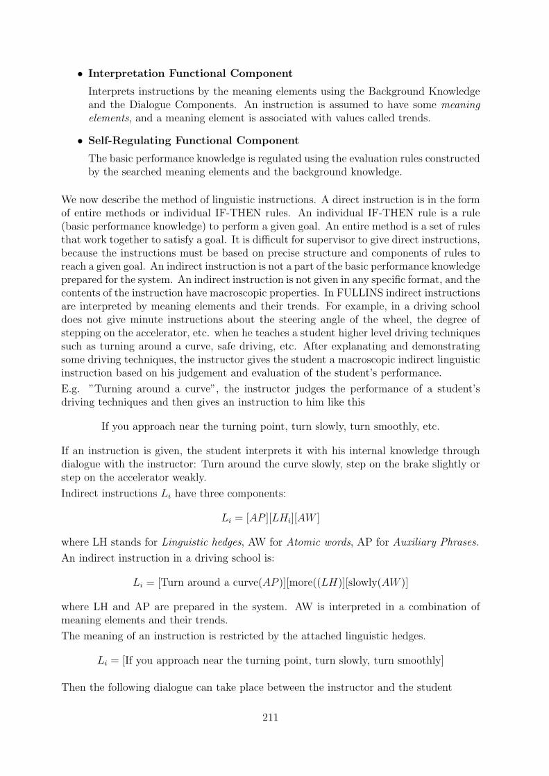
• Interpretation Functional Component
Interprets instructions by the meaning elements using the Background Knowledgeand the Dialogue Components. An instruction is assumed to have some meaningelements, and a meaning element is associated with values called trends.
• Self-Regulating Functional Component
The basic performance knowledge is regulated using the evaluation rules constructedby the searched meaning elements and the background knowledge.
We now describe the method of linguistic instructions. A direct instruction is in the formof entire methods or individual IF-THEN rules. An individual IF-THEN rule is a rule(basic performance knowledge) to perform a given goal. An entire method is a set of rulesthat work together to satisfy a goal. It is difficult for supervisor to give direct instructions,because the instructions must be based on precise structure and components of rules toreach a given goal. An indirect instruction is not a part of the basic performance knowledgeprepared for the system. An indirect instruction is not given in any specific format, and thecontents of the instruction have macroscopic properties. In FULLINS indirect instructionsare interpreted by meaning elements and their trends. For example, in a driving schooldoes not give minute instructions about the steering angle of the wheel, the degree ofstepping on the accelerator, etc. when he teaches a student higher level driving techniquessuch as turning around a curve, safe driving, etc. After explanating and demonstratingsome driving techniques, the instructor gives the student a macroscopic indirect linguisticinstruction based on his judgement and evaluation of the student’s performance.
E.g. ”Turning around a curve”, the instructor judges the performance of a student’sdriving techniques and then gives an instruction to him like this
If you approach near the turning point, turn slowly, turn smoothly, etc.
If an instruction is given, the student interprets it with his internal knowledge throughdialogue with the instructor: Turn around the curve slowly, step on the brake slightly orstep on the accelerator weakly.
Indirect instructions Li have three components:
Li = [AP ][LHi][AW ]
where LH stands for Linguistic hedges, AW for Atomic words, AP for Auxiliary Phrases.
An indirect instruction in a driving school is:
Li = [Turn around a curve(AP )][more((LH)][slowly(AW )]
where LH and AP are prepared in the system. AW is interpreted in a combination ofmeaning elements and their trends.
The meaning of an instruction is restricted by the attached linguistic hedges.
Li = [If you approach near the turning point, turn slowly, turn smoothly]
Then the following dialogue can take place between the instructor and the student
211
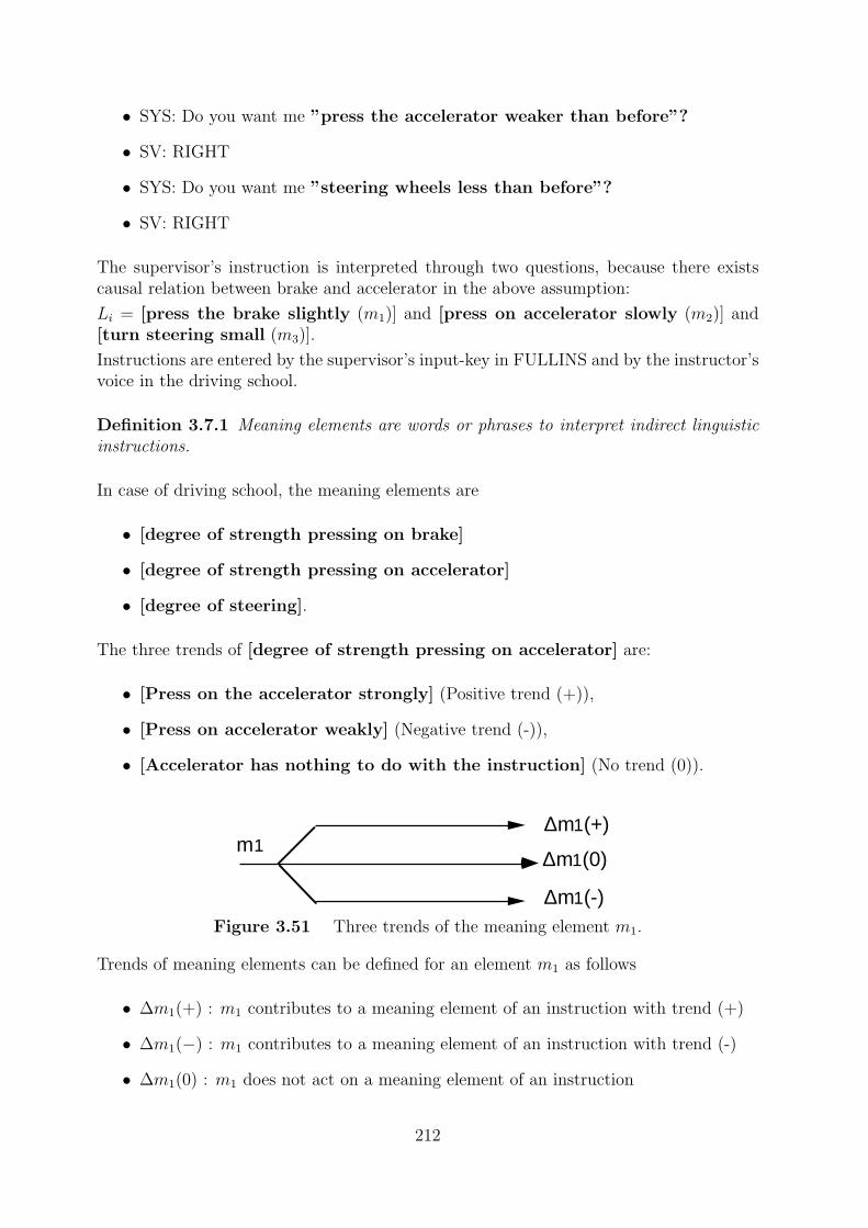
m1∆m1(+)
∆m1(-)
∆m1(0)
• SYS: Do you want me ”press the accelerator weaker than before”?
• SV: RIGHT
• SYS: Do you want me ”steering wheels less than before”?
• SV: RIGHT
The supervisor’s instruction is interpreted through two questions, because there existscausal relation between brake and accelerator in the above assumption:
Li = [press the brake slightly (m1)] and [press on accelerator slowly (m2)] and[turn steering small (m3)].
Instructions are entered by the supervisor’s input-key in FULLINS and by the instructor’svoice in the driving school.
Definition 3.7.1 Meaning elements are words or phrases to interpret indirect linguisticinstructions.
In case of driving school, the meaning elements are
• [degree of strength pressing on brake]
• [degree of strength pressing on accelerator]
• [degree of steering].
The three trends of [degree of strength pressing on accelerator] are:
• [Press on the accelerator strongly] (Positive trend (+)),
• [Press on accelerator weakly] (Negative trend (-)),
• [Accelerator has nothing to do with the instruction] (No trend (0)).
Figure 3.51 Three trends of the meaning element m1.
Trends of meaning elements can be defined for an element m1 as follows
• ∆m1(+) : m1 contributes to a meaning element of an instruction with trend (+)
• ∆m1(−) : m1 contributes to a meaning element of an instruction with trend (-)
• ∆m1(0) : m1 does not act on a meaning element of an instruction
212
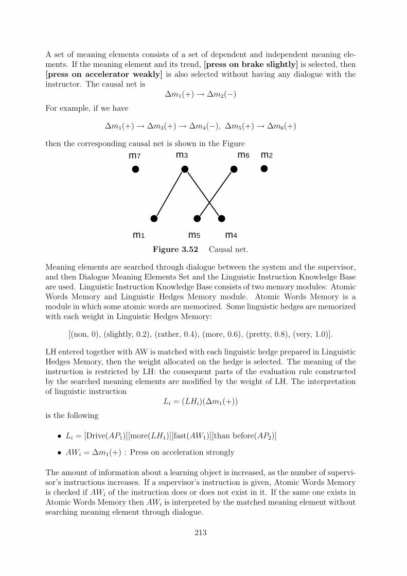
m7
m5m1
m3 m6 m2
m4
A set of meaning elements consists of a set of dependent and independent meaning ele-ments. If the meaning element and its trend, [press on brake slightly] is selected, then[press on accelerator weakly] is also selected without having any dialogue with theinstructor. The causal net is
∆m1(+)→ ∆m2(−)
For example, if we have
∆m1(+)→ ∆m3(+)→ ∆m4(−), ∆m5(+)→ ∆m6(+)
then the corresponding causal net is shown in the Figure
Figure 3.52 Causal net.
Meaning elements are searched through dialogue between the system and the supervisor,and then Dialogue Meaning Elements Set and the Linguistic Instruction Knowledge Baseare used. Linguistic Instruction Knowledge Base consists of two memory modules: AtomicWords Memory and Linguistic Hedges Memory module. Atomic Words Memory is amodule in which some atomic words are memorized. Some linguistic hedges are memorizedwith each weight in Linguistic Hedges Memory:
[(non, 0), (slightly, 0.2), (rather, 0.4), (more, 0.6), (pretty, 0.8), (very, 1.0)].
LH entered together with AW is matched with each linguistic hedge prepared in LinguisticHedges Memory, then the weight allocated on the hedge is selected. The meaning of theinstruction is restricted by LH: the consequent parts of the evaluation rule constructedby the searched meaning elements are modified by the weight of LH. The interpretationof linguistic instruction
Li = (LHi)(∆m1(+))
is the following
• Li = [Drive(AP1)][more(LH1)][fast(AW1)][than before(AP2)]
• AWi = ∆m1(+) : Press on acceleration strongly
The amount of information about a learning object is increased, as the number of supervi-sor’s instructions increases. If a supervisor’s instruction is given, Atomic Words Memoryis checked if AWi of the instruction does or does not exist in it. If the same one exists inAtomic Words Memory then AWi is interpreted by the matched meaning element withoutsearching meaning element through dialogue.
213
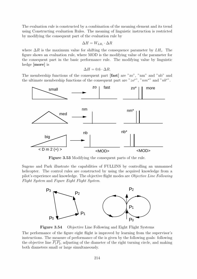
small fastzo zo* more
mednm nm*
bignb nb*
<MOD> <MOD>< D m 2 (+) >
P1
P2P3
P0 P0
P2
P1
The evaluation rule is constructed by a combination of the meaning element and its trendusing Constructing evaluation Rules. The meaning of linguistic instruction is restrictedby modifying the consequent part of the evaluation rule by
∆H = WLHi ·∆Rwhere ∆R is the maximum value for shifting the consequence parameter by LHi. Thefigure shows an evaluation rule, where MOD is the modifying value of the parameter forthe consequent part in the basic performance rule. The modifying value by linguistichedge [more] is
∆H = 0.6 ·∆R.The membership functions of the consequent part [fast] are ”zo”, ”nm” and ”nb” andthe ultimate membership functions of the consequent part are ”zo∗”, ”nm∗” and ”nb∗”.
Figure 3.53 Modifying the consequent parts of the rule.
Sugeno and Park illustrate the capabilities of FULLINS by controlling an unmannedhelicopter. The control rules are constructed by using the acquired knowledge from apilot’s experience and knowledge. The objective flight modes are Objective Line FollowingFlight System and Figure Eight Flight System.
Figure 3.54 Objective Line Following and Eight Flight Systems
The performance of the figure eight flight is improved by learning from the supervisor’sinstructions. The measure of performance of the is given by the following goals: followingthe objective line P1P2, adjusting of the diameter of the right turning circle, and makingboth diameters small or large simultaneously.
214
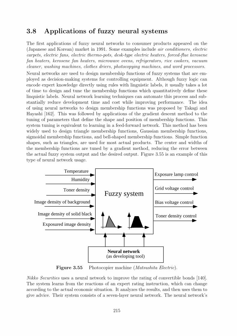
Temperature
Humidity
Toner density
Image density of solid black
Image density of background
Exposured image density
Exposure lamp control
Grid voltage control
Bias voltage control
Toner density control
Neural network(as developing tool)
Fuzzy system
3.8 Applications of fuzzy neural systems
The first applications of fuzzy neural networks to consumer products appeared on the(Japanese and Korean) market in 1991. Some examples include air conditioners, electriccarpets, electric fans, electric thermo-pots, desk-type electric heaters, forced-flue kerosenefan heaters, kerosene fan heaters, microwave ovens, refrigerators, rice cookers, vacuumcleaner, washing machines, clothes driers, photocopying machines, and word processors.
Neural networks are used to design membership functions of fuzzy systems that are em-ployed as decision-making systems for controlling equipment. Although fuzzy logic canencode expert knowledge directly using rules with linguistic labels, it usually takes a lotof time to design and tune the membership functions which quantitatively define theselinquistic labels. Neural network learning techniques can automate this process and sub-stantially reduce development time and cost while improving performance. The ideaof using neural networks to design membership functions was proposed by Takagi andHayashi [162]. This was followed by applications of the gradient descent method to thetuning of parameters that define the shape and position of membership functions. Thissystem tuning is equivalent to learning in a feed-forward network. This method has beenwidely used to design triangle membership functions, Gaussian membership functions,sigmoidal membership functions, and bell-shaped membership functions. Simple functionshapes, such as triangles, are used for most actual products. The center and widths ofthe membership functions are tuned by a gradient method, reducing the error betweenthe actual fuzzy system output and the desired output. Figure 3.55 is an example of thistype of neural network usage.
Figure 3.55 Photocopier machine (Matsushita Electric).
Nikko Securities uses a neural network to improve the rating of convertible bonds [140].The system learns from the reactions of an expert rating instruction, which can changeaccording to the actual economic situation. It analyzes the results, and then uses them togive advice. Their system consists of a seven-layer neural network. The neural network’s
215
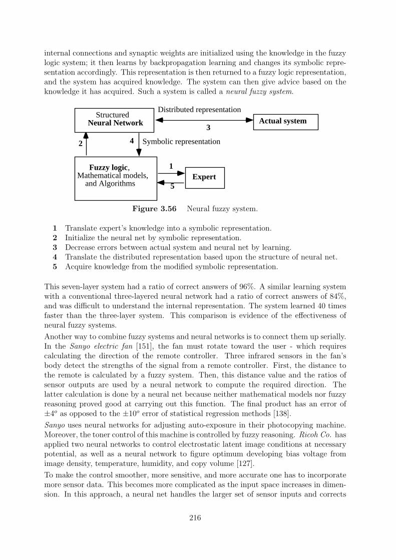
StructuredNeural Network Actual system
Expert1
5
Symbolic representation2 4
3
Distributed representation
Fuzzy logic,Mathematical models, and Algorithms
internal connections and synaptic weights are initialized using the knowledge in the fuzzylogic system; it then learns by backpropagation learning and changes its symbolic repre-sentation accordingly. This representation is then returned to a fuzzy logic representation,and the system has acquired knowledge. The system can then give advice based on theknowledge it has acquired. Such a system is called a neural fuzzy system.
Figure 3.56 Neural fuzzy system.
1 Translate expert’s knowledge into a symbolic representation.2 Initialize the neural net by symbolic representation.3 Decrease errors between actual system and neural net by learning.4 Translate the distributed representation based upon the structure of neural net.5 Acquire knowledge from the modified symbolic representation.
This seven-layer system had a ratio of correct answers of 96%. A similar learning systemwith a conventional three-layered neural network had a ratio of correct answers of 84%,and was difficult to understand the internal representation. The system learned 40 timesfaster than the three-layer system. This comparison is evidence of the effectiveness ofneural fuzzy systems.
Another way to combine fuzzy systems and neural networks is to connect them up serially.In the Sanyo electric fan [151], the fan must rotate toward the user - which requirescalculating the direction of the remote controller. Three infrared sensors in the fan’sbody detect the strengths of the signal from a remote controller. First, the distance tothe remote is calculated by a fuzzy system. Then, this distance value and the ratios ofsensor outputs are used by a neural network to compute the required direction. Thelatter calculation is done by a neural net because neither mathematical models nor fuzzyreasoning proved good at carrying out this function. The final product has an error of±4o as opposed to the ±10o error of statistical regression methods [138].
Sanyo uses neural networks for adjusting auto-exposure in their photocopying machine.Moreover, the toner control of this machine is controlled by fuzzy reasoning. Ricoh Co. hasapplied two neural networks to control electrostatic latent image conditions at necessarypotential, as well as a neural network to figure optimum developing bias voltage fromimage density, temperature, humidity, and copy volume [127].
To make the control smoother, more sensitive, and more accurate one has to incorporatemore sensor data. This becomes more complicated as the input space increases in dimen-sion. In this approach, a neural net handles the larger set of sensor inputs and corrects
216
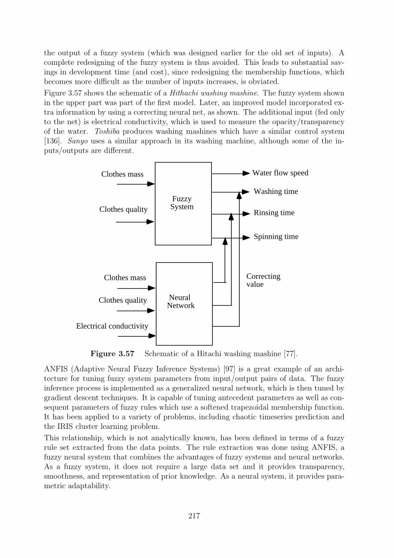
Clothes mass
Clothes quality
Clothes mass
Clothes quality
Water flow speed
Washing time
Rinsing time
Spinning time
Correctingvalue
NeuralNetwork
FuzzySystem
Electrical conductivity
the output of a fuzzy system (which was designed earlier for the old set of inputs). Acomplete redesigning of the fuzzy system is thus avoided. This leads to substantial sav-ings in development time (and cost), since redesigning the membership functions, whichbecomes more difficult as the number of inputs increases, is obviated.
Figure 3.57 shows the schematic of a Hithachi washing mashine. The fuzzy system shownin the upper part was part of the first model. Later, an improved model incorporated ex-tra information by using a correcting neural net, as shown. The additional input (fed onlyto the net) is electrical conductivity, which is used to measure the opacity/transparencyof the water. Toshiba produces washing mashines which have a similar control system[136]. Sanyo uses a similar approach in its washing machine, although some of the in-puts/outputs are different.
Figure 3.57 Schematic of a Hitachi washing mashine [77].
ANFIS (Adaptive Neural Fuzzy Inference Systems) [97] is a great example of an archi-tecture for tuning fuzzy system parameters from input/output pairs of data. The fuzzyinference process is implemented as a generalized neural network, which is then tuned bygradient descent techniques. It is capable of tuning antecedent parameters as well as con-sequent parameters of fuzzy rules which use a softened trapezoidal membership function.It has been applied to a variety of problems, including chaotic timeseries prediction andthe IRIS cluster learning problem.
This relationship, which is not analytically known, has been defined in terms of a fuzzyrule set extracted from the data points. The rule extraction was done using ANFIS, afuzzy neural system that combines the advantages of fuzzy systems and neural networks.As a fuzzy system, it does not require a large data set and it provides transparency,smoothness, and representation of prior knowledge. As a neural system, it provides para-metric adaptability.
217
Bibliography
[1] S. Abe and M.-S. Lan, A classifier using fuzzy rules extracted directly fromnumerical data, in: Proceedings of IEEE Internat. Conf. on Fuzzy Systems, SanFrancisco,1993 1191-1198.
[2] S. Abe and M.-S. Lan, Fuzzy rules extraction directly from numerical data forfunction approximation, IEEE Trans. Syst., Man, and Cybernetics, 25(1995)119-129.
[3] S. Abe and M.-S. Lan, A method for fuzzy rule extraction directly from nu-merical data and its application to pattern classification, IEEE Transactions onFuzzy Systems, 3(1995) 18-28.
[4] F. Aminzadeh and M. Jamshidi eds., Fuzzy Sets, Neural Networks, and Dis-tributed Artificial Intelligence (Prentice-Hall, Englewood Cliffs, 1994).
[5] P.E. An, S. Aslam-Mir, M. Brown, and C.J. Harris, A reinforcement learningapproach to on-line optimal control, in: Proc. of IEEE International Conferenceon Neural Networks, Orlando, Fl, 1994 2465–2471.
[6] K. Asakawa and H. Takagi, Neural Networks in Japan Communications of ACM,37(1994) 106-112.
[7] K.. Asai, M. Sugeno and T. Terano, Applied Fuzzy Systems (Academic Press,New York, 1994).
[8] A. Bastian, Handling the nonlinearity of a fuzzy logic controller at the transitionbetween rules, Fuzzy Sets and Systems, 71(1995) 369-387.
[9] H.R. Berenji, A reinforcement learning-based architecture for fuzzy logic control,Int. Journal Approximate Reasoning, 6(1992) 267-292.
[10] H.R. Berenji and P. Khedkar, Learning and tuning fuzzy logic controllersthrough reinforcements, IEEE Transactions on Neural Networks, 3(1992) 724-740.
[11] H.R. Berenji, R.N. Lea, Y. Jani, P. Khedkar, A.Malkani and J. Hoblit, Spaceshuttle attitude control by reinforcement learning and fuzzy logic, in: Proc.IEEE Internat. Conf. on Fuzzy Systems, San Francisco,1993 1396-1401.
[12] H.R. Berenji, Fuzzy systems that can learn, in: J.M. Zurada, R.J. Marks andC.J. Robinson eds., Computational Intelligence: Imitating Life (IEEE Press,New York, 1994) 23-30.
218
[13] J.C. Bezdek, E.C. Tsao and N.K. Pal, Fuzzy Kohonen clustering networks, in:Proc. IEEE Int. Conference on Fuzzy Systems 1992, San Diego, 1992 1035–1043.
[14] J.C. Bezdek and S.K. Pal eds., Fuzzy Models for Pattern Recognition (IEEEPress, New York, 1992).
[15] S.A. Billings, H.B. Jamaluddin, and S. Chen. Properties of neural networks withapplication to modelling nonlinear systems, Int. J. Control, 55(1992)193–224.
[16] A. Blanco, M. Delgado and I. Requena, Improved fuzzy neural networks forsolving relational equations, Fuzzy Sets and Systems, 72(1995) 311-322.
[17] M. Brown and C.J. Harris, A nonlinear adaptive controller: A comparison be-tween fuzzy logic control and neurocontrol. IMA J. Math. Control and Info.,8(1991) 239–265.
[18] M. Brown and C. Harris, Neurofuzzy Adaptive Modeling and Control (Prentice-Hall, Englewood Cliffs, 1994).
[19] J.J. Buckley, Theory of the fuzzy controller: An introduction, Fuzzy Sets andSystems, 51(1992) 249-258.
[20] J.J. Buckley and Y. Hayashi, Fuzzy neural nets and applications, Fuzzy Systemsand AI, 1(1992) 11-41.
[21] J.J. Buckley, Approximations between nets, controllers, expert systems andprocesses, in: Proceedings of 2nd Internat. Conf. on Fuzzy Logic and NeuralNetworks, Iizuka, Japan, 1992 89-90.
[22] J.J. Buckley, Y. Hayashi and E. Czogala, On the equivalence of neural nets andfuzzy expert systems, Fuzzy Sets and Systems, 53(1993) 129-134.
[23] J.J.Buckley, Sugeno type controllers are universal controllers, Fuzzy Sets andSystems, 53(1993) 299-304.
[24] J.J. Buckley and Y. Hayashi, Numerical relationships between neural networks,continuous functions, and fuzzy systems, Fuzzy Sets and Systems, 60(1993) 1-8.
[25] J.J. Buckley and Y. Hayashi, Hybrid neural nets can be fuzzy controllers andfuzzy expert systems, Fuzzy Sets and Systems, 60(1993) 135-142.
[26] J.J. Buckley and E. Czogala, Fuzzy models, fuzzy controllers and neural nets,Arch. Theoret. Appl. Comput. Sci., 5(1993) 149-165.
[27] J.J. Buckley and Y. Hayashi, Can fuzzy neural nets approximate continuousfuzzy functions? Fuzzy Sets and Systems, 61(1993) 43-51.
[28] J.J .Buckley and Y. Hayashi, Fuzzy neural networks, in: L.A. Zadeh andR.R. Yager eds., Fuzzy Sets, Neural Networks and Soft Computing (Van Nos-trand Reinhold, New York, 1994) 233-249.
[29] J.J .Buckley and Y. Hayashi, Fuzzy neural networks: A survey, Fuzzy Sets andSystems, 66(1994) 1-13.
219
[30] J.J .Buckley and Y. Hayashi, Neural nets for fuzzy systems, Fuzzy Sets andSystems, 71(1995) 265-276.
[31] G.A.Capenter et al, Fuzzy ARTMAP: A neural network architecture for incre-mental supervised learning of analog multidimensional maps, IEEE Transac-tions on Neural Networks, 3(1992) 698-713.
[32] S. Chen, S.A. Billings, and P.M. Grant, Recursive hybrid algorithm for non-linear system identification using radial basis function networks, Int. J. Control,55(1992) 1051–1070.
[33] F.C. Chen and M.H. Lin, On the learning and convergence of radial basis net-works, in: Proc. IEEE Int. Conf. Neural Networks, San Francisco, 1993 983–988.
[34] E. Cox, Adaptive fuzzy systems, IEEE Spectrum, , February 1993, 27–31.
[35] E. Cox, The Fuzzy system Handbook. A Practitioner’s Guide to Building, Using,and Maintaining Fuzzy Systems (Academic Press, New York, 1994).
[36] D. Dumitrescu, Fuzzy training procedures I, Fuzzy Sets and Systems, 56(1993)155-169.
[37] P. Eklund, H. Virtanen and T. Riisssanen, On the fuzzy logic nature of neuralnets, in: Proccedings of Neuro-Nimes, 1991 293–300.
[38] P. Eklund and F. Klawonn, A Formal Framework for Fuzzy Logic Based Diagno-sis, in: R.Lowen and M.Roubens eds., Proccedings of the Fourth IFSA Congress,vol. Mathematics, Brussels, 1991, 58-61.
[39] P. Eklund, M. Fogstrom and J. Forsstrom, A Generic Neuro-Fuzzy Toolfor Developing Medical Decision Support, in: P.Eklund ed., ProceedingsMEPP92,International Seminar on Fuzzy Control through Neural Interpreta-tions of Fuzzy Sets (Abo Akademis tryckeri, Abo, 1992) 1–27.
[40] P. Eklund, F. Klawonn, and D. Nauck, Distributing errors in neural fuzzy con-trol. in: Proc. 2nd Internat Conf. on Fuzzy Logic and Neural Networks, Iizuka,Japan, 1992 1139–1142.
[41] P. Eklund and F. Klawonn, Neural fuzzy logic programming, IEEE transactionson Neural Networks 3(1992) 815-818.
[42] P. Eklund, Neural Logic: A Basis for Second Generation Fuzzy Controllers, in:U.Hohle and E.P.Klement eds., Proceedings of 14th Linz Seminar on Fuzzy SetTheory, Johannes Kepler Universitat, 1992 19-23.
[43] P. Eklund and R. Fuller, A neuro-fuzzy approach to medical diagnostics,in:Proceedings of EUFIT’93 Conference, September 7-10, 1993, Aachen, Ger-many (Verlag der Augustinus Buchhandlung, Aachen, 1993) 810-813.
[44] P. Eklund, J. Forsstrom, A. Holm, M.. Nystrom, and G. Selen, Rule generationas an alternative to knowledge acquisition: A systems architecture for medicalinformatics, Fuzzy Sets and Systems, 66(1994) 195-205.
220
[45] P. Eklund, Network size versus preprocessing, in: R.R. Yager and L.A. Zadeheds., Fuzzy Sets, Neural Networks and Soft Computing (Van Nostrand, NewYork, 1994) 250-264.
[46] P. Eklund, A generic system for developing medical decision support, FuzzySystems A.I. Rep. Letters, 3(1994) 71-78.
[47] P. Eklund and J. Forsstrom, Computational intelligence for laboratory informa-tion systems, Scand. J. Clin. Lab. Invest., 55 Suppl. 222 (1995) 75-82.
[48] A.O. Esogbue, A fuzzy adaptive controller using reinforcement learning neuralnetworks, in: Proc. IEEE Internat. Conf. on Fuzzy Systems, San Francisco,1993178–183.
[49] J. Forsstrom, P. Eklund, H. Virtanen, J. Waxlax and J. Lahdevirta, DiagaiD: AConnectionists Approach to Determine the Information Value of Clinical Data,Artificial Intelligence in Medicine, 3 (1991) 193-201.
[50] T. Fukuda and T. Shibata, Fuzzy-neuro-GA based intelligent robotics, in:J.M. Zurada, R.J. Marks and C.J. Robinson eds., Computational Intelligence:Imitating Life (IEEE Press, New York, 1994) 352-363.
[51] M. Furukawa and T. Yamakawa, The design algorithms of membership functionsfor a fuzzy neuron, Fuzzy Sets and Systems, 71(1995) 329-343.
[52] S. Gallant, Neural Network Learning and Expert Systems, MIT Press, Cam-bridge, Mass., USA, 1993
[53] A. Geyer-Schulz, Fuzzy rule based Expert Systems and Genetic Learning(Physica-Verlag, Berlin, 1995).
[54] S. Giove, M. Nordio and A. Zorat, An Adaptive Fuzzy Control for AutomaticDialysis, in: E.P. Klement and W. Slany eds., Fuzzy Logic in Artificial Intelli-gence, (Springer-Verlag, Berlin 1993) 146-156.
[55] P.Y. Glorennec, Learning algorithms for neuro-fuzzy networks, in: A. Kandeland G. Langholz eds., Fuzzy Control Systems (CRC Press, New York, 1994)4-18.
[56] A. Gonzalez, R. Perez and J.L. Verdegay, Learning the structure of a fuzzy rule:A genetic approach, Fuzzy Systems A.I.Rep. Letters, 3(1994) 57-70.
[57] S. Goonatilake and S. Khebbal eds., Intelligent Hybrid Systems, John Wiley andSons, New York 1995.
[58] M.M. Gupta and J. Qi, On fuzzy neuron models, in: Proceedings of InternationalJoint Conference on Neural Networks, Seattle, 1991 431-436.
[59] M.M. Gupta and J. Qi, On fuzzy neuron models, in: L.A. Zadeh and J. Kacprzykeds., Fuzzy Logic for the Management of Uncertainty (J. Wiley, New York, 1992)479-491.
221
[60] M.M. Gupta, Fuzzy logic and neural networks, Proc. 2nd Internat. Conf. onFuzzy logic and Neural Networks, Iizuka, Japan, 1992 157-160.
[61] M.M. Gupta and M.B. Gorzalczany, Fuzzy neuro-computation technique and itsapplication to modeling and control, in: Proc. IEEE Internat. Conf on FuzzySystems, San Diego, 1992 1271-1274.
[62] M.M. Gupta and D.H. Rao, On the principles of fuzzy neural networks, FuzzySets and Systems, 59(1993) 271-279.
[63] S.K. Halgamuge and M. Glesner, Neural networks in designing fuzzy systemsfor real world applications, Fuzzy Sets and Systems, 65(1994) 1-12.
[64] C.J. Harris, C.G. Moore, and M. Brown, Intelligent control, aspects of fuzzylogic and neural networks (World Scientific Press, 1993).
[65] C.J. Harris ed., Advances in Intelligent Control (Taylor and Francis, London,1994).
[66] Y. Hayashi, J.J. Buckley and E. Czogala, Systems engineering applications offuzzy neural networks, Journal of Systems Engineering, 2(1992) 232-236.
[67] Y. Hayashi, J.J. Buckley and E. Czogala, Fuzzy neural controller, in: Proc.IEEE Internat. Conf on Fuzzy Systems, San Diego, 1992 197-202.
[68] Y. Hayashi, H. Nomura, H. Yamasaki and N. Wakami, Construction of fuzzyinference rules by NFD and NDFL, International Journal of Approximate Rea-soning, 6(1992) 241-266.
[69] Y. Hayashi, Neural expert system using fuzzy teaching input, in: Proc. IEEEInternat. Conf on Fuzzy Systems, San Diego, 1992 485-491.
[70] Y. Hayashi, J.J. Buckley and E. Czogala, Fuzzy neural network with fuzzysignals and weight, International Journal of Intelligent Systems, 8(1992) 527-537.
[71] Y. Hayashi, J.J. Buckley and E. Czogala, Direct fuzzification of neural networkand fuzzified delta rule, Proc. 2nd Internat. Conf. on Fuzzy logic and NeuralNetworks, Iizuka, Japan, 1992 73-76.
[72] Y. Hayashi and J.J. Buckley, Direct fuzzification of neural networks, in: Pro-ceedings of 1st Asian Fuzzy Systems Symposium, Singapore, 1993 560-567.
[73] Y. Hayashi and J.J. Buckley, Approximations between fuzzy expert systems andneural networks, International Journal of Approximate Reasoning, 10(1994) 63-73.
[74] K. Hirota and W. Pedrycz, Knowledge-based networks in classification problems,Fuzzy Sets and Systems, 51(1992) 1-27.
[75] K. Hirota and W. Pedrycz, OR/AND neuron in modeling fuzzy set connectives,IEEE Transactions on Fuzzy Systems, 2(994) 151-161.
222
[76] K. Hirota and W. Pedrycz, Fuzzy modelling environment for designing fuzzycontrollers, Fuzzy Sets and Systems, 70(1995) 287-301.
[77] Hitachi, Neuro and fuzzy logic automatic washing machine and fuzzy logic drier,Hitachi News Rel., No. 91-024 (Feb. 26, 1991). Hitachi, 1991 (in Japanese).
[78] S. Horikowa, T. Furuhashi and Y. Uchikawa, On fuzzy modeling using fuzzyneural networks with the backpropagation algorithm, IEEE Transactions onNeural Networks, 3(1992).
[79] S. Horikowa, T. Furuhashi and Y. Uchikawa, On identification of structuresin premises of a fuzzy model using a fuzzy neural network, in: Proc. IEEEInternational Conference on Fuzzy Systems, San Francisco, 1993 661-666.
[80] K.J. Hunt, D. Sbarbaro-Hofer, R. Zbikowski and P.J. Gawthrop, Neural net-works for control systems - a survey, Automatica, 28(1992) 1083–1112.
[81] H. Ichihashi, Iterative fuzzy modelling and a hierarchical network, in: R.Lowenand M.Roubens eds., Proceedings of the Fourth IFSA Congress, Vol. Engineer-ing, Brussels, 1991 49-52.
[82] H. Ishibuchi, R. Fujioka and H. Tanaka, An architecture of neural networksfor input vectors of fuzzy numbers, in: Proc. IEEE Internat. Conf on FuzzySystems, San Diego, 1992 1293-1300.
[83] H. Ishibuchi, K. Nozaki and H. Tanaka, Distributed representation of fuzzy rulesand its application to pattern classification, Fuzzy Sets and Systems, 52(1992)21-32.
[84] H. Ishibuchi and H. Tanaka, Approximate pattern classification using neuralnetworks, in: R.Lowen and M.Roubens eds., Fuzzy Logic: State of the Art(Kluwer, Dordrecht, 1993) 225-236.
[85] H. Ishibuchi, K. Nozaki and H. Tanaka, Efficient fuzzy partition of pattern spacefor classification problems, Fuzzy Sets and Systems, 59(1993) 295-304.
[86] H. Ishibuchi, R. Fujioka and H. Tanaka, Neural networks that learn from fuzzyIF-THEN rules, IEEE Transactions on Fuzzy Systems, 1(993) 85-97.
[87] H. Ishibuchi, H. Okada and H. Tanaka, Fuzzy neural networks with fuzzy weightsand fuzzy biases, in: Proc. IEEE Internat. Conference on Neural Networks, SanFrancisco, 1993 447-452.
[88] H. Ishibuchi, K. Kwon and H. Tanaka, Implementation of fuzzy IF-THEN rulesby fuzzy neural networks with fuzzy weights, in: Proceedings of EUFIT’93 Con-ference, September 7-10, 1993 Aachen, Germany, Verlag der Augustinus Buch-handlung, Aachen, 1993 209-215.
[89] H. Ishibuchi, K. Kwon and H. Tanaka, Learning of fuzzy neural networks fromfuzzy inputs and fuzzy targets, in: Proc. 5th IFSA World Congress, Seoul,Korea, 1993 147-150.
223
[90] H. Ishibuchi, K. Nozaki and H. Tanaka, Empirical study on learning in fuzzysystems, in: Proc. 2nd IEEE Internat. Conference on Fuzzy Systems, San Fran-cisco, 1993 606-611.
[91] H. Ishibuchi, K. Nozaki, N. Yamamato and H. Tanaka, Genetic operations forrule selection in fuzzy classification systems, in: Proc. 5th IFSA World Congress,Seoul, Korea, 1993 15-18.
[92] H. Ishibuchi, K. Nozaki, N. Yamamato, Selecting fuzzy rules by genetic algo-rithm for classification problems, in: Proc. 2nd IEEE Internat. Conference onFuzzy Systems, San Francisco, 1993 1119-1124.
[93] H. Ishibuchi, H. Okada and H. Tanaka, Interpolation of fuzzy IF-THEN rulesby neural networks, International Journal of Approximate Reasoning, 10(1994)3-27.
[94] H. Ishibuchi, K. Nozaki, N. Yamamato and H. Tanaka, Construction of fuzzyclassification systems with rectangular fuzzy rules using genetic algorithms,Fuzzy Sets and Systems, 65(1994) 237-253.
[95] H. Ishibuchi, K. Kwon and H. Tanaka, A learning algorithm of fuzzy neuralnetworks with triangular fuzzy weights, Fuzzy Sets and Systems, 71(1995) 277-293.
[96] H. Ishigami, T. Fukuda, T. Shibita and F. Arai, Structure optimization of fuzzyneural network by genetic algorithm, Fuzzy Sets and Systems, 71(1995) 257-264.
[97] J.-S. Roger Jang, ANFIS: Adaptive-network-based fuzzy inference system, IEEETrans. Syst., Man, and Cybernetics, 23(1993) 665-685.
[98] J.M. Keller and D. Hunt, Incorporating fuzzy membership functions into theperceptron algorithm, IEEE Transactions on Pattern. Anal. Mach. Intell.,7(1985) 693-699.
[99] J.M. Keller, R.R. Yager and H.Tahani, Neural network implementation of fuzzylogic, Fuzzy Sets and Systems, 45(1992) 1-12.
[100] J.M. Keller and H.Tahani, Backpropagation neural networks for fuzzy logic,Information Sciences, 6(1992) 205-221.
[101] J.M. Keller and H.Tahani, Implementation of conjunctive and disjunctive fuzzylogic rules with neural networks, International Journal of Approximate Reason-ing, 6(1992) 221-240.
[102] J.M. Keller, R. Krishnapuram, Z.H. Chen and O. Nasraoui, Fuzzy additivehybrid operators for network-based decision making, International Journal ofIntelligent Systems 9(1994) 1001-1023.
[103] E. Khan and P. Venkatapuram, Neufuz: Neural network based fuzzy logic designalgorithms, in: Proceedings of IEEE International Conf. on Fuzzy Systems, SanFrancisco, 1993 647–654.
224
[104] P.S. Khedkar, Learning as adaptive interpolation in neural fuzzy systems, in:J.M. Zurada, R.J. Marks and C.J. Robinson eds., Computational Intelligence:Imitating Life (IEEE Press, New York, 1994) 31-42.
[105] Y.S. Kim and S. Mitra, An adaptive integrated fuzzy clustering model for pat-tern recognition, Fuzzy Sets and Systems, 65(1994) 297-310.
[106] S.G. Kong and B. Kosko, Adaptive fuzzy systems for backing up a truck-and-trailer, IEEE Transactions on Neural Networks, 3(1992) 211-223.
[107] B. Kosko, Neural Networks and Fuzzy Systems (Prentice-Hall, Englewood Cliffs,1992).
[108] R. Krishnapuram and J. Lee, Fuzzy-set-based hierarchical networks for infor-mation fusion in computer vision, Neural Networks, 5(1992) 335-350.
[109] R. Kruse, J. Gebhardt and R. Palm eds., Fuzzy Systems in Computer Science(Vieweg, Braunschweig, 1994).
[110] D.C. Kuncicky, A fuzzy interpretation of neural networks, in: Proceedings of3rd IFSA Congress, 1989 113–116.
[111] H.K. Kwan and Y.Cai, A fuzzy neural network and its application to patternrecognition, IEEE Transactions on Fuzzy Systems, 3(1994) 185-193.
[112] S.C. Lee and E.T. Lee, Fuzzy sets and neural networks, Journal of Cybernetics4(1974) 83-103.
[113] S.C. Lee and E.T. Lee, Fuzzy neural networks, Math. Biosci. 23(1975) 151-177.
[114] H.-M. Lee and W.-T. Wang, A neural network architecture for classification offuzzy inputs, Fuzzy Sets and Systems, 63(1994) 159-173.
[115] M. Lee, S.Y. Lee and C.H. Park, Neuro-fuzzy identifiers and controllers, J. ofIntelligent Fuzzy Systems, 6(1994) 1-14.
[116] K.-M. Lee, D.-H. Kwang and H.L. Wang, A fuzzy neural network model forfuzzy inference and rule tuning,International Journal of Uncertainty, Fuzzinessand Knowledge-Based Systems, 3(1994) 265-277.
[117] C.T. Lin and C.S.G. Lee, Neural-network-based fuzzy logic control and decisionsystem, IEEE Transactions on Computers, 40(1991) 1320-1336.
[118] Y. Lin and G.A. Cunningham III, A new approach to fuzzy-neural system mod-eling, IEEE Transactions on Fuzzy systems, 3(1995) 190-198.
[119] C.T. Lin and Y.C. Lu, A neural fuzzy system with linguistic teaching signals,IEEE Transactions on Fuzzy Systems, 3(1995) 169-189.
[120] R.J. Machado and A.F. Rocha, A hybrid architecture for fuzzy connectionistexpert systems, in: A. Kandel and G. Langholz eds., Hybrid Architectures forIntelligent Systems (CRC Press, Boca Raton, FL, 1992).
225
[121] R.A. Marques Pereira, L. Mich and L. Gaio, Curve reconstruction with dynam-ical fuzzy grading and weakly continuous constraints, in: Proceedings of the 2ndWorkshop on Current Issues in Fuzzy Technologies, Trento, June 1992, (Dipar-timento di Informatica e Studi Aziendali, Universita di Trento 1993) 77-85.
[122] L. Medsker, Hybrid Neural Network and Expert Systems (Kluwer Academic Pub-lishers, Boston, 1994).
[123] S.Mitra and S.K.Pal, Neuro-fuzzy expert systems: overview with a case study,in: S.Tzafestas and A.N. Venetsanopoulos eds., Fuzzy Reasoning in Information,Decision and Control Systems ( Kluwer, Dordrecht, 1994) 121-143.
[124] S.Mitra and S.K.Pal, Self-organizing neural network as a fuzzy classifier, IEEETrans. Syst., Man, and Cybernetics, 24(1994) 385-399.
[125] S.Mitra and S.K.Pal, Fuzzy multi-layer perceptron, inferencing and rule gener-ation, IEEE Transactions on Neural Networks, 6(1995) 51-63.
[126] S.Mitra, Fuzzy MLP based expert system for medical diagnosis, Fuzzy sets andSystems, 65(1994) 285-296.
[127] T. Morita, M. Kanaya and T. Inagaki, Photo-copier image density control usingneural network and fuzzy theory. in: Proceedings of the Second InternationalWorkshop on Industrial Fuzzy Control and Intelligent Systems, 1992 10-16.
[128] D. Nauck, F. Klawonn and R. Kruse, Fuzzy sets, fuzzy controllers and neu-ral networks,Wissenschaftliche Zeitschrift der Humboldt-Universitat zu Berlin,reihe Medizin, 41(1992) 99-120.
[129] D. Nauck and R. Kruse, A fuzzy neural network learning fuzzy control rules andmembership functions by fuzzy error backpropagation, in: Proceedings of IEEEInt. Conference on Neural Networks, San Francisco, 1993 1022-1027.
[130] D. Nauck, F. Klawonn and R. Kruse, Combining neural networks and fuzzycontrollers, in: E.P. Klement and W. Slany eds., Fuzzy Logic in Artificial Intel-ligence, (Springer-Verlag, Berlin, 1993) 35-46.
[131] D. Nauck and R. Kruse, NEFCON-I: An X-Window based simulator for neuralfuzzy controllers, in: Proceedings of IEEE Int. Conference on Neural Networks,Orlando, 1994 1638-1643.
[132] D. Nauck, Fuzzy neuro systems: An overview, in: R. Kruse, J. Gebhardt andR. Palm eds., Fuzzy systems in Computer Science (Vieweg, Wiesbaden, 1994)91-107.
[133] D. Nauck, Building neural fuzzy controllers with NEFCON-I. in: R. Kruse,J. Gebhardt and R. Palm eds., Fuzzy systems in Computer Science (Vieweg,wiesbaden, 1994) 141-151.
[134] D. Nauck, F. Klawonn and R. Kruse, Neurale Netze und Fuzzy-Systeme (Vieweg,wiesbaden, 1994).
226
[135] D. Nauck and R. Kruse, NEFCLASS - A neuro-fuzzy approach for the classifi-cation of data, in: K.M. George et al eds., Applied Computing, Proceedings ofthe 1995 ACM Symposium on Applied Computing, Nashville, February 26-28,1995, ACM Press, 1995.
[136] R. Narita, H. Tatsumi and H. Kanou, Application of neural networks to house-hold applications. Toshba Rev. 46, 12 (December 1991) 935-938. (in Japanese)
[137] J. Nie and D. Linkens, Fuzzy Neural Control - Principles, Algorithms and Ap-plications (Prentice-Hall, Englewood Cliffs, 1994).
[138] Nikkei Electronics, New trend in consumer electronics: Combining neural net-works and fuzzy logic, Nikkei Elec., 528(1991) 165-169 (In Japanese).
[139] H. Nomura, I. Hayashi and N. Wakami, A learning method of fuzzy inferencerules by descent method, in: Proceedings of the IEEE International Conferenceon Fuzzy Systems, San Diego, 1992 203-210.
[140] H. Okada, N. Watanabe, A. Kawamura and K. Asakawa, Initializing multilayerneural networks with fuzzy logic. in: Proceedings of the International JointConference on Neural Networks, Baltimore, 1992 239-244.
[141] S.K.Pal and S.Mitra, Fuzzy versions of Kohonen’s net and MLP-based classi-fication: Performance evaluation for certain nonconvex decision regions, Infor-mation Sciences, 76(1994) 297-337.
[142] W. Pedrycz and W.C. Card, Linguistic interpretation of self-organizing maps,in: Proceedings of the IEEE International Conference on Fuzzy Systems, SanDiego, 1992 371–378.
[143] W. Pedrycz, Fuzzy Control and Fuzzy Systems (Wiley, New York, 1993).
[144] W. Pedrycz, Fuzzy Sets Engineering (CRC Press, Boca Raton, 1995).
[145] C. Posey, A.Kandel and G. Langholz, Fuzzy hybrid systems, in: A. Kandel andG. Langholz eds., Hybrid architectures for Intelligent Systems (CRC Press, BocaRaton, Florida, 1992) 174-196.
[146] G.V.S. Rajau and J Zhou, Adaptive hierarchical fuzzy controller, IEEE Trans.Syst., Man, and Cybernetics, 23(1993) 973-980.
[147] A.L. Ralescu ed., Fuzzy Logic in Artificial Intelligence, Proc. IJCAI’93 Work-shop, Chambery, France, Lecture Note in artificial Intelligence, Vol. 847(Springer, Berlin, 1994).
[148] J. Rasmussen, Diagnostic reasoning in action, IEEE Trans. Syst., Man, andCybernetics, 23(1993) 981-992.
[149] I. Requena and M. Delgado, R-FN: A model of fuzzy neuron, in: Proc. 2nd Int.Conf. on Fuzzy Logic & Neural Networks, Iizuka, Japan, 1992 793-796.
227
[150] T. Riissanen, An Experiment with Clustering, Proceedings MEPP92, Interna-tional Seminar on Fuzzy Control through Neural Interpretations of Fuzzy Sets,Mariehamn, Aland, June 15-19, 1992, Abo Akademi tryckeri, Abo, 1992, 57-65.
[151] Sanyo, Electric fan series in 1991, Sanyo News Rel., (March 14, 1991). Sanyo,1991 (In Japanese).
[152] E. Sanchez, Fuzzy logic knowledge systems and artificial neural networks inmedicine and biology, in: R.R. Yager and L.A. Zadeh eds., An Introduction toFuzzy Logic Applications in Intelligent Systems (Kluwer, Boston, 1992) 235-251.
[153] J.D. Schaffer, Combinations of genetic algorithms with neural networks or fuzzysystems, in: J.M. Zurada, R.J. Marks and C.J. Robinson eds., ComputationalIntelligence: Imitating Life (IEEE Press, New York, 1994) 371-382.
[154] R. Serra and G. Zanarini, Complex Systems and Cognitive Processes (SpringerVerlag, Berlin, 1990).
[155] J.J. Shann and H.C. Fu, A fuzzy neural network for rule acquiring on fuzzycontrol system, Fuzzy Sets and Systems, 71(1995) 345-357.
[156] P. Simpson, Fuzzy min-max neural networks: 1.Classification, IEEE Transac-tions on Neural Networks, 3(1992) 776-786.
[157] P. Simpson, Fuzzy min-max neural networks: 2.Clustering, IEEE Transactionson Fuzzy systems, 1(1993) 32-45.
[158] M. Sugeno and G.-K. Park, An approach to linguistic instruction based learning,International Journal of Uncertainty, Fuzziness and Knowledge-Based Systems,1(1993) 19-56.
[159] S.M. Sulzberger, N.N.Tschichold-Gurman and S.J. Vestli, FUN: Optimization offuzzy rule based systems using neural networks, in: Proc. IEEE Int. Conferenceon Neural Networks, San Francisco, 1993 312–316.
[160] C.-T. Sun and J.-S. Jang, A neuro-fuzzy classifier and its applications, in: Proc.IEEE Int. Conference on Neural Networks, San Francisco, 1993 94–98.
[161] H. Takagi, Fusion technology of fuzzy theory and neural networks - survey andfuture directions, in: Proc. First Int. Conf. on Fuzzy Logic & Neural Networks,1990 13–26.
[162] H. Takagi and I. Hayashi, NN-driven fuzzy reasoning. International Journal ofApproximate Reasoning, 3(1991) 191-212.
[163] H. Takagi, N. Suzuki, T. Koda and Y. Kojima, neural networks designed onapproximate reasoning architecture and their applications, IEEE Transactionson Neural Networks, 3(1992) 752-760.
[164] I.B.Turksen, Fuzzy expert systems for IE/OR/MS, Fuzzy Sets and Systems,51(1992) 1-27.
228
[165] K. Uehara and M. Fujise, Learning of fuzzy inference criteria with artificialneural network, in: Proc. 1st Int. Conf. on Fuzzy Logic & Neural Networks,Iizuka, Japan, 1990 193-198.
[166] M. Umano and Y, Ezawa, Execution of approximate reasoning by neural net-work, Proceedings of FAN Symposium, 1991 267-273 (in Japanese).
[167] H. Virtanen, Combining and incrementing fuzzy evidence - Heuristic and for-mal approaches to fuzzy logic programming, in: R.Lowen and M.Roubens eds.,Proccedings of the fourth IFSA Congress, vol. Mathematics, Brussels, 1991 200-203.
[168] L.-X. Wang and J.M. Mendel, Generating fuzzy rules by learning from examples,IEEE Trans. Syst., Man, and Cybernetics, 22(1992) 1414-1427.
[169] H. Watanabe et al., Application of fuzzy discriminant analysis for diagnosis ofvalvular heart disease, IEEE Transactions on Fuzzy Systems, 2(1994) 267- 276.
[170] P.J. Werbos, Neurocontrol and fuzzy logic: connections and designs, Interna-tional Journal of Approximate Reasoning, 6(1992) 185-219.
[171] R.R. Yager, Using fuzzy logic to build neural networks, in: R.Lowen andM.Roubens eds., Proceedings of the Fourth IFSA Congress, Vol. Artifical in-telligence, Brussels, 1991 210-213.
[172] R.R. Yager, Implementing fuzzy logic controllers using a neural network frame-work, Fuzzy Sets and Systems, 48(1992) 53-64.
[173] R.R. Yager and L.A. Zadeh eds., Fuzzy Sets, Neural Networks, and Soft Com-puting (Van Nostrand Reinhold, New York, 1994).
[174] T. Yamakawa, A neo fuzzy neuron and its applications to system identifica-tion and prediction of chaotic behaviour, in: J.M. Zurada, R.J. Marks andC.J. Robinson eds., Computational Intelligence: Imitating Life (IEEE Press,New York, 1994) 383-395.
[175] J. Yan, M. Ryan and J. Power, Using Fuzzy Logic - Towards Intelligent Systems(Prentice-Hall, Englewood Cliffs, 1994).
[176] Y. Yam and K.S. Leung eds., Future Directions of Fuzzy Theory and Systems(World Scientific, Singapore, 1994).
229
Chapter 4
Appendix
4.1 Case study: A portfolio problem
Suppose that our portfolio value depends on the currency fluctations on the global financemarket. There are three rules in our knowledge base:
<1 : if x1 is L1 and x2 is H2 and x3 is L3 then y = 200x1 + 100x2 + 100x3
<2 : if x1 is M1 and x2 is M2 and x3 is M3 then y = 200x1 − 100x2 + 100x3
<3 : if x1 is H1 and x2 is H2 and x3 is H3 then y = 200x1 − 100x2 − 100x3
where y is the portfolio value, the linguistic variables x1, x2 and x3 denote the exchangerates between USD and DEM, USD and SEK, and USD and FIM, respectively.
The rules should be interpreted as:
<1 : If the US dollar is weak against German mark and the US dollar is strong againstthe Swedish crown and the US dollar is weak against the Finnish mark then ourportfolio value is positive.
<2 : If the US dollar is medium against German mark and the US dollar is mediumagainst the Swedish crown and the US dollar is medium against the Finnish markthen our portfolio value is about zero.
<3 : If the US dollar is strong against German mark and the US dollar is strong againstthe Swedish crown and the US dollar is strong against the Finnish mark then ourportfolio value is negative.
Choose triangular membership functions for primary fuzzy sets {Li,Mi, Hsi}, i = 1, 2, 3,take the actual daily exchange rates, a1, a2 and a3, from newspapers and evaluate thedaily portfolio value by Sugeno’s reasoning mechanism, i.e.
• The firing levels of the rules are computed by
α1 = L1(a1) ∧H2(a2) ∧ L3(a3),
α2 = M1(a1) ∧M2(a2) ∧M3(a3),
α3 = H1(a1) ∧H2(a2) ∧H3(a3),
230
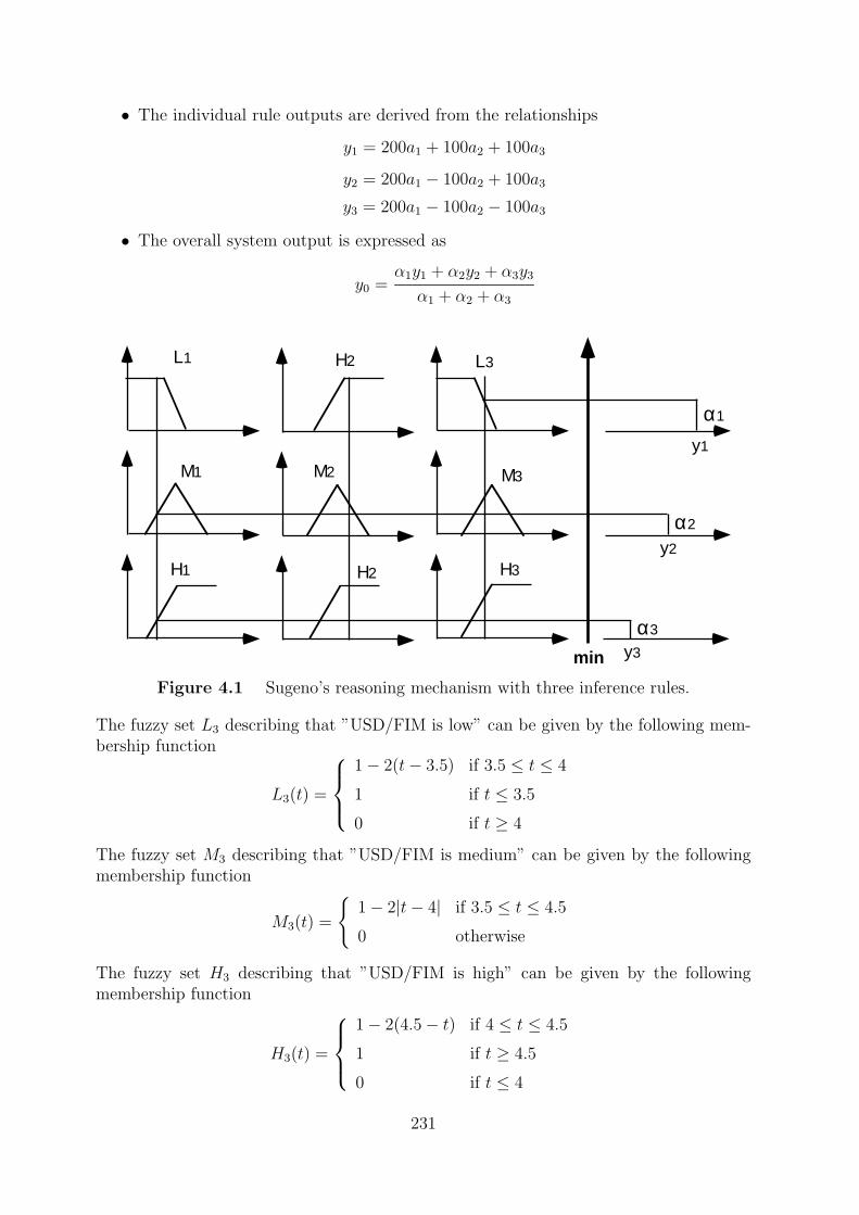
min
α1
α2
L1 L3H2
M1 M3M2
H1 H3
α3
y1
y3
y2
H2
• The individual rule outputs are derived from the relationships
y1 = 200a1 + 100a2 + 100a3
y2 = 200a1 − 100a2 + 100a3
y3 = 200a1 − 100a2 − 100a3
• The overall system output is expressed as
y0 =α1y1 + α2y2 + α3y3
α1 + α2 + α3
Figure 4.1 Sugeno’s reasoning mechanism with three inference rules.
The fuzzy set L3 describing that ”USD/FIM is low” can be given by the following mem-bership function
L3(t) =
1− 2(t− 3.5) if 3.5 ≤ t ≤ 4
1 if t ≤ 3.5
0 if t ≥ 4
The fuzzy set M3 describing that ”USD/FIM is medium” can be given by the followingmembership function
M3(t) =
{1− 2|t− 4| if 3.5 ≤ t ≤ 4.5
0 otherwise
The fuzzy set H3 describing that ”USD/FIM is high” can be given by the followingmembership function
H3(t) =
1− 2(4.5− t) if 4 ≤ t ≤ 4.5
1 if t ≥ 4.5
0 if t ≤ 4
231
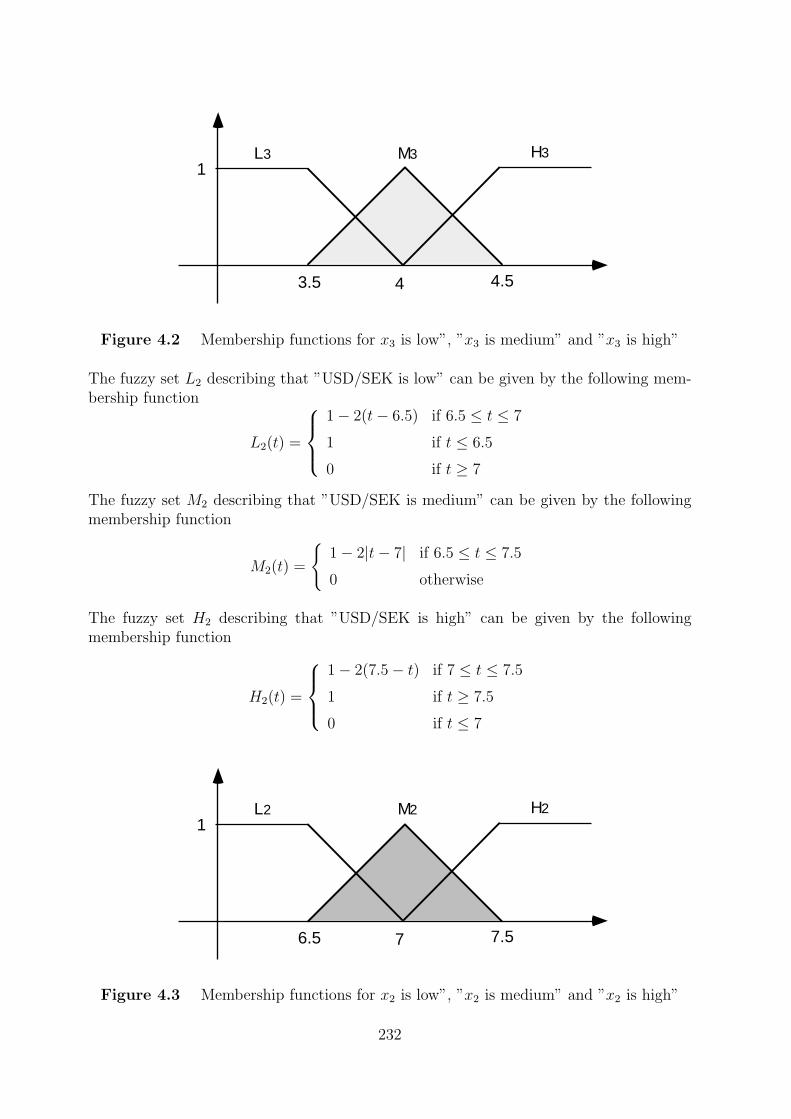
3.5 4 4.5
1H3L3 M3
6.5 7 7.5
1H2L2 M2
Figure 4.2 Membership functions for x3 is low”, ”x3 is medium” and ”x3 is high”
The fuzzy set L2 describing that ”USD/SEK is low” can be given by the following mem-bership function
L2(t) =
1− 2(t− 6.5) if 6.5 ≤ t ≤ 7
1 if t ≤ 6.5
0 if t ≥ 7
The fuzzy set M2 describing that ”USD/SEK is medium” can be given by the followingmembership function
M2(t) =
{1− 2|t− 7| if 6.5 ≤ t ≤ 7.5
0 otherwise
The fuzzy set H2 describing that ”USD/SEK is high” can be given by the followingmembership function
H2(t) =
1− 2(7.5− t) if 7 ≤ t ≤ 7.5
1 if t ≥ 7.5
0 if t ≤ 7
Figure 4.3 Membership functions for x2 is low”, ”x2 is medium” and ”x2 is high”
232
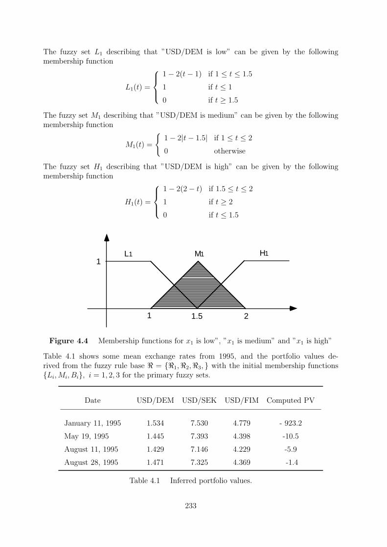
1 1.5 2
1H1L1 M1
The fuzzy set L1 describing that ”USD/DEM is low” can be given by the followingmembership function
L1(t) =
1− 2(t− 1) if 1 ≤ t ≤ 1.5
1 if t ≤ 1
0 if t ≥ 1.5
The fuzzy set M1 describing that ”USD/DEM is medium” can be given by the followingmembership function
M1(t) =
{1− 2|t− 1.5| if 1 ≤ t ≤ 2
0 otherwise
The fuzzy set H1 describing that ”USD/DEM is high” can be given by the followingmembership function
H1(t) =
1− 2(2− t) if 1.5 ≤ t ≤ 2
1 if t ≥ 2
0 if t ≤ 1.5
Figure 4.4 Membership functions for x1 is low”, ”x1 is medium” and ”x1 is high”
Table 4.1 shows some mean exchange rates from 1995, and the portfolio values de-rived from the fuzzy rule base < = {<1,<2,<3, } with the initial membership functions{Li,Mi, Bi}, i = 1, 2, 3 for the primary fuzzy sets.
Date USD/DEM USD/SEK USD/FIM Computed PV
January 11, 1995 1.534 7.530 4.779 - 923.2
May 19, 1995 1.445 7.393 4.398 -10.5
August 11, 1995 1.429 7.146 4.229 -5.9
August 28, 1995 1.471 7.325 4.369 -1.4
Table 4.1 Inferred portfolio values.
233
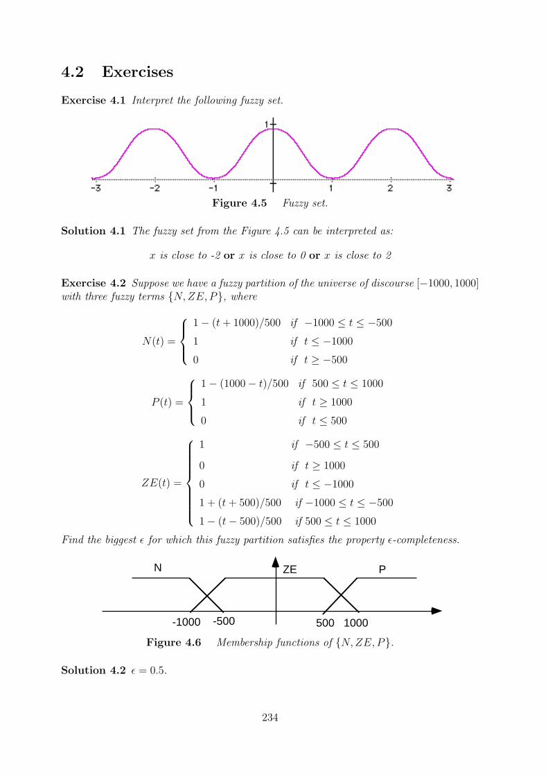
1000-1000
PN ZE
-500 500
4.2 Exercises
Exercise 4.1 Interpret the following fuzzy set.
Figure 4.5 Fuzzy set.
Solution 4.1 The fuzzy set from the Figure 4.5 can be interpreted as:
x is close to -2 or x is close to 0 or x is close to 2
Exercise 4.2 Suppose we have a fuzzy partition of the universe of discourse [−1000, 1000]with three fuzzy terms {N,ZE, P}, where
N(t) =
1− (t+ 1000)/500 if −1000 ≤ t ≤ −500
1 if t ≤ −1000
0 if t ≥ −500
P (t) =
1− (1000− t)/500 if 500 ≤ t ≤ 1000
1 if t ≥ 1000
0 if t ≤ 500
ZE(t) =
1 if −500 ≤ t ≤ 500
0 if t ≥ 1000
0 if t ≤ −1000
1 + (t+ 500)/500 if −1000 ≤ t ≤ −500
1− (t− 500)/500 if 500 ≤ t ≤ 1000
Find the biggest ε for which this fuzzy partition satisfies the property ε-completeness.
Figure 4.6 Membership functions of {N,ZE, P}.
Solution 4.2 ε = 0.5.
234
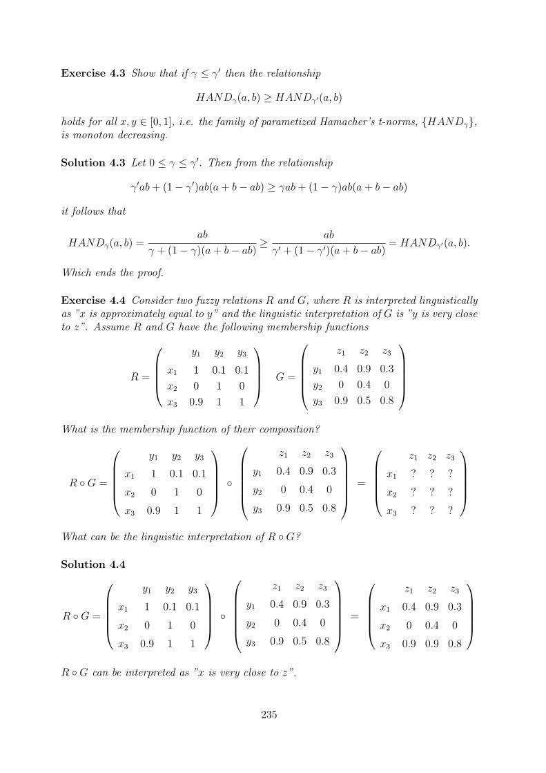
Exercise 4.3 Show that if γ ≤ γ′ then the relationship
HANDγ(a, b) ≥ HANDγ′(a, b)
holds for all x, y ∈ [0, 1], i.e. the family of parametized Hamacher’s t-norms, {HANDγ},is monoton decreasing.
Solution 4.3 Let 0 ≤ γ ≤ γ′. Then from the relationship
γ′ab+ (1− γ′)ab(a+ b− ab) ≥ γab+ (1− γ)ab(a+ b− ab)
it follows that
HANDγ(a, b) =ab
γ + (1− γ)(a+ b− ab) ≥ab
γ′ + (1− γ′)(a+ b− ab) = HANDγ′(a, b).
Which ends the proof.
Exercise 4.4 Consider two fuzzy relations R and G, where R is interpreted linguisticallyas ”x is approximately equal to y” and the linguistic interpretation of G is ”y is very closeto z”. Assume R and G have the following membership functions
R =
y1 y2 y3
x1 1 0.1 0.1
x2 0 1 0
x3 0.9 1 1
G =
z1 z2 z3
y1 0.4 0.9 0.3
y2 0 0.4 0
y3 0.9 0.5 0.8
What is the membership function of their composition?
R ◦G =
y1 y2 y3
x1 1 0.1 0.1
x2 0 1 0
x3 0.9 1 1
◦
z1 z2 z3
y1 0.4 0.9 0.3
y2 0 0.4 0
y3 0.9 0.5 0.8
=
z1 z2 z3
x1 ? ? ?
x2 ? ? ?
x3 ? ? ?
What can be the linguistic interpretation of R ◦G?
Solution 4.4
R ◦G =
y1 y2 y3
x1 1 0.1 0.1
x2 0 1 0
x3 0.9 1 1
◦
z1 z2 z3
y1 0.4 0.9 0.3
y2 0 0.4 0
y3 0.9 0.5 0.8
=
z1 z2 z3
x1 0.4 0.9 0.3
x2 0 0.4 0
x3 0.9 0.9 0.8
R ◦G can be interpreted as ”x is very close to z”.
235
Exercise 4.5 Assume the membership function of the fuzzy set A, big pressure is
A(u) =
1 if u ≥ 5
1− (5− u)/4 if 1 ≤ u ≤ 5
0 otherwise
Assume the membership function of the fuzzy set B, small volume is
B(v) =
1 if v ≤ 1
1− (v − 1)/4 if 1 ≤ v ≤ 5
0 otherwise
What is the truth value of the proposition?
”4 is big pressure”→ ”3 is small volume”
where → is the ÃLukasiewicz implication.
Solution 4.5 Using the definition of ÃLukasiewicz implication we get
”4 is big pressure”→ ”3 is small volume” ≡ A(4)→ B(3) = min{1− A(4) +B(3), 1}
and from A(4) = 0.75 and B(3) = 0.5 we get
”4 is big pressure”→ ”3 is small volume” = min{1− 0.75 + 0.5, 1} = 0.75
Exercise 4.6 Let A, A′, B ∈ F . Show that the Generalized Modus Ponens inferencerule with Godel implication satisfies
• Basic property: A ◦ (A→ B) = B
• Total indeterminance: ¬A ◦ (A→ B) = 1 where 1(t) = 1 for t ∈ IR
• Subset property: If A′ ⊂ A then A′ ◦ (A→ B) = B
• Superset property: A′ ◦ (A→ B) = B′ ⊂ B holds for any A′ ∈ F .
Solution 4.6 The Generalized Modus Ponens inference rule says
premise if x is A then y is Bfact x is A′
consequence: y is B′
where the consequence B′ is determined as a composition of the fact and the fuzzy impli-cation operator
B′ = A′ ◦ (A→ B)
that is,B′(v) = sup
u∈Umin{A′(u), (A→ B)(u, v)}, v ∈ V.
236
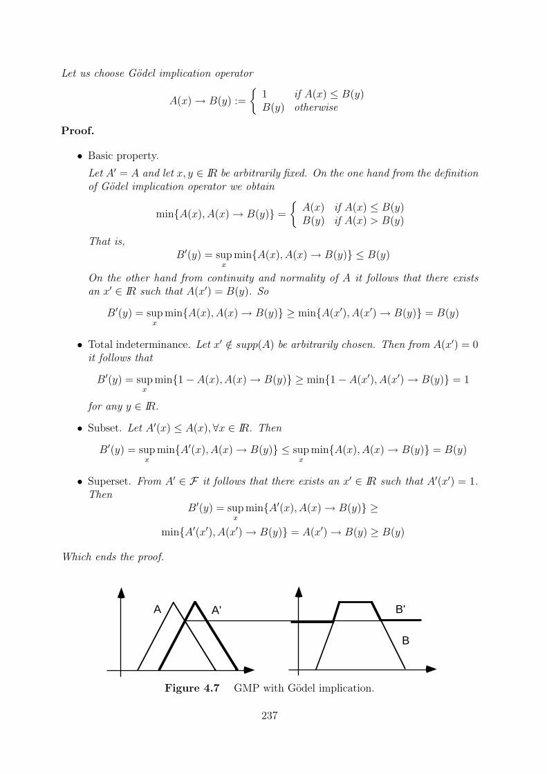
A B'
B
A'
Let us choose Godel implication operator
A(x)→ B(y) :=
{1 if A(x) ≤ B(y)B(y) otherwise
Proof.
• Basic property.
Let A′ = A and let x, y ∈ IR be arbitrarily fixed. On the one hand from the definitionof Godel implication operator we obtain
min{A(x), A(x)→ B(y)} =
{A(x) if A(x) ≤ B(y)B(y) if A(x) > B(y)
That is,B′(y) = sup
xmin{A(x), A(x)→ B(y)} ≤ B(y)
On the other hand from continuity and normality of A it follows that there existsan x′ ∈ IR such that A(x′) = B(y). So
B′(y) = supx
min{A(x), A(x)→ B(y)} ≥ min{A(x′), A(x′)→ B(y)} = B(y)
• Total indeterminance. Let x′ /∈ supp(A) be arbitrarily chosen. Then from A(x′) = 0it follows that
B′(y) = supx
min{1− A(x), A(x)→ B(y)} ≥ min{1− A(x′), A(x′)→ B(y)} = 1
for any y ∈ IR.
• Subset. Let A′(x) ≤ A(x), ∀x ∈ IR. Then
B′(y) = supx
min{A′(x), A(x)→ B(y)} ≤ supx
min{A(x), A(x)→ B(y)} = B(y)
• Superset. From A′ ∈ F it follows that there exists an x′ ∈ IR such that A′(x′) = 1.Then
B′(y) = supx
min{A′(x), A(x)→ B(y)} ≥
min{A′(x′), A(x′)→ B(y)} = A(x′)→ B(y) ≥ B(y)
Which ends the proof.
Figure 4.7 GMP with Godel implication.
237
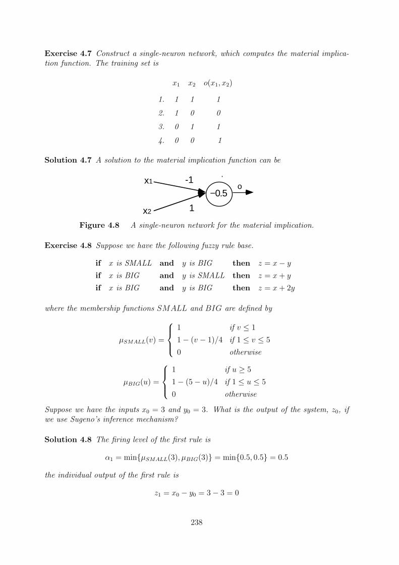
x1
x2
ο-1
1
−0.5
Exercise 4.7 Construct a single-neuron network, which computes the material implica-tion function. The training set is
x1 x2 o(x1, x2)
1. 1 1 1
2. 1 0 0
3. 0 1 1
4. 0 0 1
Solution 4.7 A solution to the material implication function can be
Figure 4.8 A single-neuron network for the material implication.
Exercise 4.8 Suppose we have the following fuzzy rule base.
if x is SMALL and y is BIG then z = x− yif x is BIG and y is SMALL then z = x+ y
if x is BIG and y is BIG then z = x+ 2y
where the membership functions SMALL and BIG are defined by
µSMALL(v) =
1 if v ≤ 1
1− (v − 1)/4 if 1 ≤ v ≤ 5
0 otherwise
µBIG(u) =
1 if u ≥ 5
1− (5− u)/4 if 1 ≤ u ≤ 5
0 otherwise
Suppose we have the inputs x0 = 3 and y0 = 3. What is the output of the system, z0, ifwe use Sugeno’s inference mechanism?
Solution 4.8 The firing level of the first rule is
α1 = min{µSMALL(3), µBIG(3)} = min{0.5, 0.5} = 0.5
the individual output of the first rule is
z1 = x0 − y0 = 3− 3 = 0
238
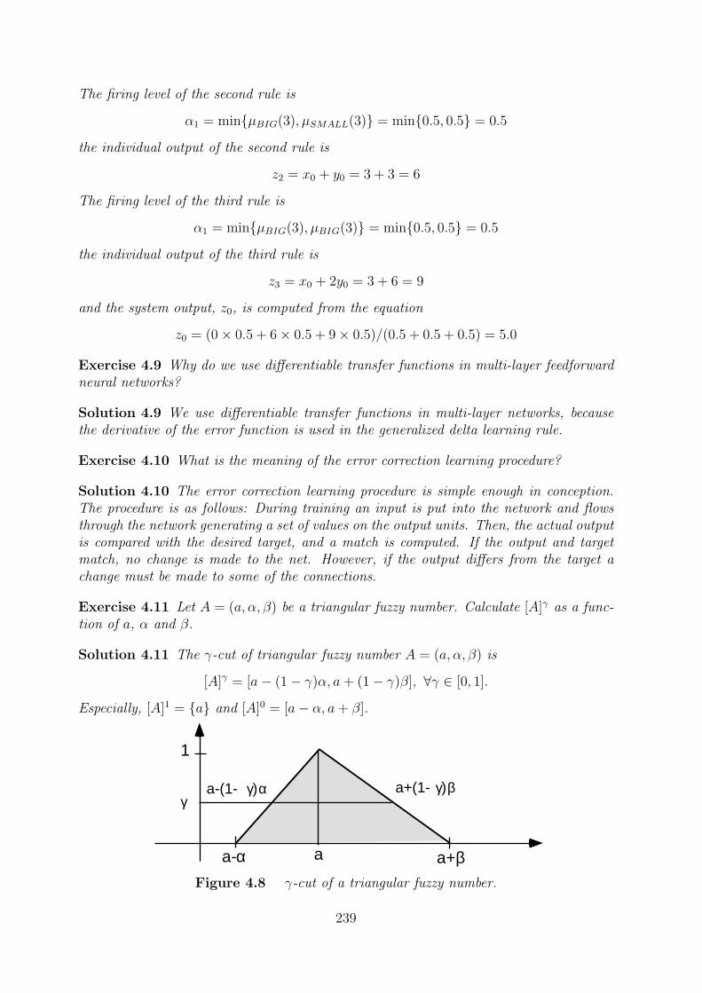
1
aa-α a+β
γa-(1- γ)α a+(1- γ)β
The firing level of the second rule is
α1 = min{µBIG(3), µSMALL(3)} = min{0.5, 0.5} = 0.5
the individual output of the second rule is
z2 = x0 + y0 = 3 + 3 = 6
The firing level of the third rule is
α1 = min{µBIG(3), µBIG(3)} = min{0.5, 0.5} = 0.5
the individual output of the third rule is
z3 = x0 + 2y0 = 3 + 6 = 9
and the system output, z0, is computed from the equation
z0 = (0× 0.5 + 6× 0.5 + 9× 0.5)/(0.5 + 0.5 + 0.5) = 5.0
Exercise 4.9 Why do we use differentiable transfer functions in multi-layer feedforwardneural networks?
Solution 4.9 We use differentiable transfer functions in multi-layer networks, becausethe derivative of the error function is used in the generalized delta learning rule.
Exercise 4.10 What is the meaning of the error correction learning procedure?
Solution 4.10 The error correction learning procedure is simple enough in conception.The procedure is as follows: During training an input is put into the network and flowsthrough the network generating a set of values on the output units. Then, the actual outputis compared with the desired target, and a match is computed. If the output and targetmatch, no change is made to the net. However, if the output differs from the target achange must be made to some of the connections.
Exercise 4.11 Let A = (a, α, β) be a triangular fuzzy number. Calculate [A]γ as a func-tion of a, α and β.
Solution 4.11 The γ-cut of triangular fuzzy number A = (a, α, β) is
[A]γ = [a− (1− γ)α, a+ (1− γ)β], ∀γ ∈ [0, 1].
Especially, [A]1 = {a} and [A]0 = [a− α, a+ β].
Figure 4.8 γ-cut of a triangular fuzzy number.
239
Exercise 4.12 Consider some alternative with the following scores on five criteria
Criteria: C1 C2 C3 C4 C5
Importance: VH VH M L VL
Score: M L OU VH OU
Calculate the unit score of this alternative.
Solution 4.12 In this case we have
U = min{Neg(V H) ∨M,Neg(V H) ∨ L,Neg(M) ∨OU,Neg(L) ∨ V H,Neg(V L) ∨OU}
= min{V L ∨M,V L ∨ L,M ∨OU,H ∨ V H, V H ∨OU} = min{M,L,OU, V H,OU} = L
Exercise 4.13 Let A = (a, α) and B = (b, β) be fuzzy numbers of symmetrical triangularform. Calculate their Hausdorff distances, D(A,B), as a function of a, b, α and β.
Solution 4.13 The γ-cuts of A and B can be written in the form
[A]γ = [a1(γ), a2(γ)] = [a− (1− γ)α, a+ (1− γ)α], ∀γ ∈ [0, 1].
[B]γ = [b1(γ), b2(γ)] = [b− (1− γ)β, b+ (1− γ)β], ∀γ ∈ [0, 1].
and from the definition of Hausdorff distance
D(A,B) = supγ∈[0,1]
max{|a1(γ)− b1(γ)|, |a2(γ)− b2(γ)|}
we get
D(A,B) = supγ∈[0,1]
max{|a− b+ (1− γ)(α− β)|, |a− b+ (1− γ)(β − α)|}
That is,D(A,B) = max{|a− b+ α− β|, |a− b+ β − α|}.
Exercise 4.14 The error function to be minimized is given by
E(w1, w2) =1
2[(w2 − w1)2 + (1− w1)2]
Find analytically the gradient vector
E ′(w) =
[∂1E(w)∂2E(w)
]Find analytically the weight vector w∗ that minimizes the error function such that
E ′(w) = 0.
Derive the steepest descent method for the minimization of E.
240
Solution 4.14 The gradient vector of E is
E ′(w) =
[(w1 − w2) + (w1 − 1)
(w2 − w1)
]=
[2w1 − w2 − 1w2 − w1
]and w∗(1, 1)T is the unique solution to the equation[
2w1 − w2 − 1w2 − w1
]=
[00
].
The steepest descent method for the minimization of E reads[w1(t+ 1)w2(t+ 1)
]= η
[2w1(t)− w2(t)− 1w2(t)− w1(t)
].
where η > 0 is the learning constant and t indexes the number of iterations. That is,
w1(t+ 1) = w1(t)− η(2w1(t)− w2(t)− 1)
w2(t+ 1) = w2(t)− η(w2(t)− w1(t))
Exercise 4.15 Let f be a bipolar sigmoidal activation function of the form
f(t) =2
1 + exp(−t)− 1.
Show that f satisfies the following differential equality
f ′(t) =1
2(1− f2(t)).
Solution 4.15 By using the chain rule for derivatives of composed functions we get
f ′(t) =2exp(−t)
[1 + exp(−t)]2.
From the identity1
2
[1−
(1− exp(−t)1 + exp(−t)
)2]=
2exp(−t)[1 + exp(−t)]2
we get2exp(−t)
[1 + exp(−t)]2 =1
2(1− f2(t)).
Which completes the proof.
Exercise 4.16 Let f be a unipolar sigmoidal activation function of the form
f(t) =1
1 + exp(−t).
Show that f satisfies the following differential equality
f ′(t) = f(t)(1− f(t)).
241
Solution 4.16 By using the chain rule for derivatives of composed functions we get
f ′(t) =exp(−t)
[1 + exp(−t)]2
and the identity
1
[1 + exp(−t)]2 =exp(−t)
1 + exp(−t)
(1−
exp(−t)1 + exp(−t)
)verifies the statement of the exercise.
Exercise 4.17 Construct a hybid neural net implementing Tsukumato’s reasoning mech-anism with two input variables, two linguistiuc values for each input variable and twofuzzy IF-THEN rules.
Solution 4.17 Consider the fuzzy rule base
<1 : if x is A1 and y is B1 then z is C1
<2 : if x is A2 and y is B2 then z is C2
where all linguistic terms are supposed to have monotonic membership functions.
The firing levels of the rules are computed by
α1 = A1(x0)×B1(y0)
α2 = A2(x0)×B2(y0),
where the logical and can be modelled by any continuous t-norm, e.g
α1 = A1(x0) ∧B1(y0)
α2 = A2(x0) ∧B2(y0),
In this mode of reasoning the individual crisp control actions z1 and z2 are computed as
z1 = C−11 (α1) and z2 = C−1
2 (α2)
and the overall control action is expressed as
z0 =α1z1 + α2z2
α1 + α2
= β1z1 + β2z2
where β1 and β1 are the normalized values of α1 and α2 with respect to the sum (α1 +α2),i.e.
β1 =α1
α1 + α2
, β2 =α2
α1 + α2
.
242
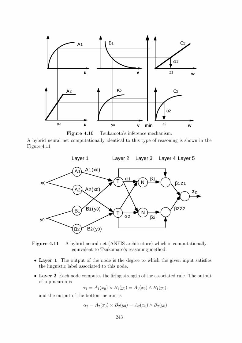
u v w
uxo vyo wmin
A1
B2
C1
A2
B1
C2
z2
z1
α2
α1
A1
A2
B1
B2
A1(x0)
A2(x0)
B1(y0)
B2(y0)
α1
α2
T
T
N
N
β1
β2
β1z1
β2z2
z0
Layer 1 Layer 2 Layer 3 Layer 4 Layer 5
x0
y0
Figure 4.10 Tsukamoto’s inference mechanism.
A hybrid neural net computationally identical to this type of reasoning is shown in theFigure 4.11
Figure 4.11 A hybrid neural net (ANFIS architecture) which is computationallyequivalent to Tsukomato’s reasoning method.
• Layer 1 The output of the node is the degree to which the given input satisfiesthe linguistic label associated to this node.
• Layer 2 Each node computes the firing strength of the associated rule. The outputof top neuron is
α1 = A1(x0)×B1(y0) = A1(x0) ∧B1(y0),
and the output of the bottom neuron is
α2 = A2(x0)×B2(y0) = A2(x0) ∧B2(y0)
243
Both nodes in this layer is labeled by T , because we can choose other t-norms formodeling the logical and operator. The nodes of this layer are called rule nodes.
• Layer 3 Every node in this layer is labeled by N to indicate the normalization ofthe firing levels.
The output of top neuron is the normalized (with respect to the sum of firing levels)firing level of the first rule
β1 =α1
α1 + α2
,
and the output of the bottom neuron is the normalized firing level of the secondrule
β2 =α2
α1 + α2
,
• Layer 4 The output of top neuron is the product of the normalized firing level andthe individual rule output of the first rule
β1z1 = β1C−11 (α1).
The output of top neuron is the product of the normalized firing level and theindividual rule output of the second rule
β2z2 = β2C−12 (α2),
• Layer 5 The single node in this layer computes the overall system output as thesum of all incoming signals, i.e.
z0 = β1z1 + β2z2.
Exercise 4.18 Show that fuzzy inference systems with simplified fuzzy IF-THEN rulesare universal approximators.
Solution 4.18 Consider a fuzzy inference systems with two simplified fuzzy IF-THENrules
<1: if x1 is A11 and x2 is A12 then y = z1
<2: if x1 is A21 and x2 is A22 then y = z2
Suppose that the output of the system < = {<1,<2} for a given input is computed by
z =α1z1 + α2z2
α1 + α2
(4.1)
where α1 and α2 denote the firing strengths of the rules with respect to given input vector.Let z′ be the output of the system < for some other input.
We recall the Stone-Weierstrass theorem:
Theorem 4.2.1 Let domain K be a compact space of n dimensions, and let G be a setof continuous real-valued functions on K, satisfying the following criteria:
244
1. The constant function f(x) = 1 is in G.
2. For any two points x1 6= x2 in K, there is an f in G such that f(x1) 6= f(x2).
3. If f1 and f2 are two functions in G, then fg and α1f1 +α2f2 are in G for any two realnumbers α1 and α2.
Then G is dense in C(K), the set of continuous real-valued functions on K. In otherwords, for any ε > 0 and any function g in C(K), there exists g in G such that
‖f − g‖∞ = supx∈K|f(x)− g(x)| ≤ ε.
Proof. We show that az + bz′, ∀a, b ∈ IR and zz′ can be written in the form (4.1)which means that fuzzy inference systems with simplified fuzzy IF-THEN rules satisfythe conditions of Stone-Weierstrass theorem, i.e. they can approximate all continuousfunctions on a compact domain.
For az + bz′ we get
az + bz′ = aα1z1 + α2z2
α1 + α2
+ bα′1z
′1 + α′2z
′2
α′1 + α′2=
a(α1z1 + α2z2)(α′1 + α′2) + b(α′1z′1 + α′2z
′2)(α1 + α2)
(α1 + α2)(α′1 + α′2)=
α1α′1(az1 + bz′1) + α1α
′2(az1 + bz′2) + α2α
′1(az2 + bz′1) + α2α
′2(az2 + bz′2)
α1α′1 + α1α′2 + α2α′1 + α2α′2
So, zz′ is the output of a fuzzy inference system with four simplified fuzzy IF-THEN,where the individual rule outputs are: az1 + bz′1, az1 + bz′2, az2 + bz′1 and az2 + bz′2, andthe firing strengths of the associated rules are α1α
′1, α1α
′2, α2α
′1 and α2α
′2, respectively.
Finally, for zz′ we obtain
zz′ =α1z1 + α2z2
α1 + α2
×α′1z
′1 + α′2z
′2
α′1 + α′2=α1α
′1z1z
′1 + α1α
′2z1z
′2 + α2α
′1z2z
′1 + α2α
′2z2z
′2
α1α′1 + α1α′2 + α2α′1 + α2α′2
So, zz′ is the output of a fuzzy inference system with four simplified fuzzy IF-THEN,where the individual rule outputs are: z1z
′1, z1z
′2, z2z
′1 and z2z
′2, and the firing strengths
of the associated rules are α1α′1, α1α
′2, α2α
′1 and α2α
′2, respectively.
Which completes the proof.
Exercise 4.19 Let A1 = (a1, α) and A2 = (a2, α) be fuzzy numbers of symmetric trian-gular form. Compute analytically the membership function of their product-sum, A1⊕A2,defined by
(A1 ⊕ A2)(y) = supx1+x2=y
PAND(A1(x1), A2(x2)) = supx1+x2=y
A1(x1)A2(x2).
Solution 4.19 The membership functions of A1 = (a1, α) and A2 = (a2, α) are definedby
245
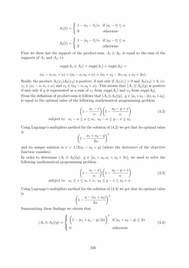
A1(t) =
{1− |a1 − t|/α if |a1 − t| ≤ α
0 otherwise
A2(t) =
{1− |a2 − t|/α if |a2 − t| ≤ α
0 otherwise
First we show hat the support of the product-sum, A1 ⊕ A2, is equal to the sum of thesupports of A1 and A2, i.e.
supp(A1 ⊕ A2) = supp(A1) + supp(A2) =
(a1 − α, a1 + α) + (a2 − α, a2 + α) = (a1 + a2 − 2α, a1 + a2 + 2α).
Really, the product A1(x1)A2(x2) is positive, if and only if A1(x1) > 0 and A2(x2) > 0, i.e.x1 ∈ (a1 − α, a1 + α) and x2 ∈ (a2 − α, a2 + α). This means that (A1 ⊕A2)(y) is positiveif and only if y is represented as a sum of x1 from supp(A1) and x2 from supp(A2).
From the definition of product-sum it follows that (A1⊕A2)(y), y ∈ [a1 +a2−2α, a1 +a2],is equal to the optimal value of the following mathematical programming problem(
1−a1 − xα
)(1−
a2 − y + x
α
)(4.2)
subject to a1 − α ≤ x ≤ a1, a2 − α ≤ y − x ≤ a2.
Using Lagrange’s multipliers method for the solution of (4.2) we get that its optimal valueis (
1−a1 + a2 − y
2α
)2
and its unique solution is x = 1/2(a1 − a2 + y) (where the derivative of the objectivefunction vanishes).
In order to determine (A1 ⊕ A2)(y), y ∈ [a1 + a2, a1 + a2 + 2α], we need to solve thefollowing mathematical programming problem(
1−a1 − xα
)(1−
a2 − y + x
α
)(4.3)
subject to a1 ≤ x ≤ a1 + α, a2 ≤ y − x ≤ a2 + α.
Using Lagrange’s multipliers method for the solution of (4.3) we get that its optimal valueis (
1−y − (a1 + a2)
2α
)2
.
Summarizing these findings we obtain that
(A1 ⊕ A2)(y) =
(
1− |a1 + a2 − y|/2α)2
if |a1 + a2 − y| ≤ 2α
0 otherwise
(4.4)
246
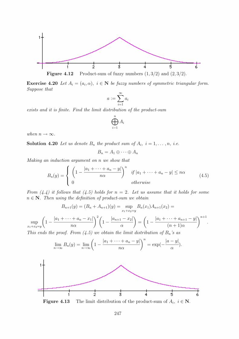
Figure 4.12 Product-sum of fuzzy numbers (1, 3/2) and (2, 3/2).
Exercise 4.20 Let Ai = (ai, α), i ∈ N be fuzzy numbers of symmetric triangular form.Suppose that
a :=∞∑i=1
ai
exists and it is finite. Find the limit distribution of the product-sumn⊕i=1
Ai
when n→∞.
Solution 4.20 Let us denote Bn the product sum of Ai, i = 1, . . . , n, i.e.
Bn = A1 ⊕ · · · ⊕ AnMaking an induction argument on n we show that
Bn(y) =
(
1−|a1 + · · ·+ an − y|
nα
)nif |a1 + · · ·+ an − y| ≤ nα
0 otherwise
(4.5)
From (4.4) it follows that (4.5) holds for n = 2. Let us assume that it holds for somen ∈ N. Then using the definition of product-sum we obtain
Bn+1(y) = (Bn + An+1)(y) = supx1+x2=y
Bn(x1)An+1(x2) =
supx1+x2=y
(1−|a1 + · · ·+ an − x1|
nα
)2(1−|an+1 − x2|
α
)=
(1−|a1 + · · ·+ an+1 − y|
(n+ 1)α
)n+1
.
This ends the proof. From (4.5) we obtain the limit distribution of Bn’s as
limn→∞
Bn(y) = limn→∞
(1−|a1 + · · ·+ an − y|
nα
)n= exp(−
|a− y|α
).
Figure 4.13 The limit distribution of the product-sum of Ai, i ∈ N.
247
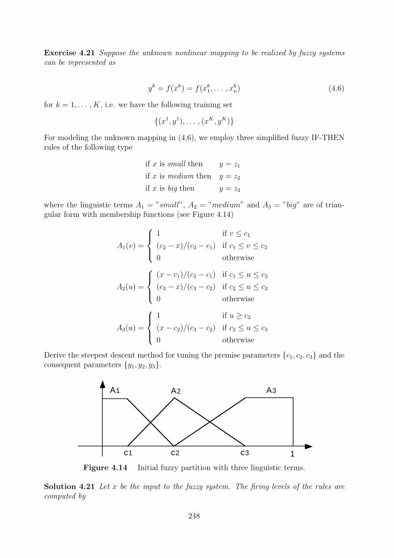
c1 c2 c3 1
A1 A2 A3
Exercise 4.21 Suppose the unknown nonlinear mapping to be realized by fuzzy systemscan be represented as
yk = f(xk) = f(xk1, . . . , xkn) (4.6)
for k = 1, . . . , K, i.e. we have the following training set
{(x1, y1), . . . , (xK , yK)}
For modeling the unknown mapping in (4.6), we employ three simplified fuzzy IF-THENrules of the following type
if x is small then y = z1
if x is medium then y = z2
if x is big then y = z3
where the linguistic terms A1 = ”small”, A2 = ”medium” and A3 = ”big” are of trian-gular form with membership functions (see Figure 4.14)
A1(v) =
1 if v ≤ c1
(c2 − x)/(c2 − c1) if c1 ≤ v ≤ c2
0 otherwise
A2(u) =
(x− c1)/(c2 − c1) if c1 ≤ u ≤ c2
(c3 − x)/(c3 − c2) if c2 ≤ u ≤ c3
0 otherwise
A3(u) =
1 if u ≥ c3
(x− c2)/(c3 − c2) if c2 ≤ u ≤ c3
0 otherwise
Derive the steepest descent method for tuning the premise parameters {c1, c2, c3} and theconsequent parameters {y1, y2, y3}.
Figure 4.14 Initial fuzzy partition with three linguistic terms.
Solution 4.21 Let x be the input to the fuzzy system. The firing levels of the rules arecomputed by
248
α1 = A1(x), α2 = A2(x), α3 = A3(x),
and the output of the system is computed by
o =α1z1 + α2z2 + α3z3
α1 + α2 + α3
=A1(x)z1 + A2(x)z2 + A3(x)z3
A1(x) + A2(x) + A3(x)= A1(x)z1 + A2(x)z2 + A3(x)z3
where we have used the identity A1(x) + A2(x) + A3(x) = 1 for all x ∈ [0, 1]. We definethe measure of error for the k-th training pattern as usually
Ek = Ek(c1, c2, c3, z1, z2, z3) =1
2(ok(c1, c2, c3, z1, z2, z3)− yk)2
where ok is the computed output from the fuzzy system corresponding to the input patternxk and yk is the desired output, k = 1, . . . , K.
The steepest descent method is used to learn zi in the consequent part of the i-th fuzzyrule. That is,
z1(t+ 1) = z1(t)− η∂Ek
∂z1
= z1(t)− η(ok − yk)A1(xk)
z2(t+ 1) = z2(t)− η∂Ek
∂z2
= z2(t)− η(ok − yk)A2(xk)
z3(t+ 1) = z3(t)− η∂Ek
∂z3
= z3(t)− η(ok − yk)A3(xk)
where xk is the input to the system, η > 0 is the learning constant and t indexes thenumber of the adjustments of zi.
In a similar manner we can tune the centers of A1, A2 and A3.
c1(t+ 1) = c1(t)− η∂Ek
∂c1
, c2(t+ 1) = c2(t)− η∂Ek
∂c2
, c3(t+ 1) = c3(t)− η∂Ek
∂c3
,
where η > 0 is the learning constant and t indexes the number of the adjustments of theparameters.
The partial derivative of the error function Ek with respect to c1 can be written as
∂Ek
∂c1
= (ok − yk)∂ok
∂c1
= (ok − yk)(x− c1)
(c2 − c1)2(z1 − z2)
if c1 ≤ xk ≤ c2, and zero otherwise.
It should be noted that the adjustments of a center can not be done independently ofother centers, because the inequality
0 ≤ c1(t+ 1) < c2(t+ 1) < c3(t+ 1) ≤ 1
must hold for all t.
249
Index
C∞ distance, 42R-implication, 47S-implication, 47α-cut, 10, 190ε-completeness, 80, 172ÃLukasiewicz t-conorm, 21ÃLukasiewicz t-norm, 20
activation function, 120, 157activation hyperbox , 202AND fuzzy neuron, 158andlike OWA operator, 94ANFIS architecture, 172ARIC architecture, 155arithmetic mean, 92artificial neuron, 119averaging operator, 91
bag, 89ball and beam system, 85basic property of GMP, 54binary fuzzy relation, 25bipolar activation function, 134
Cartesian product, 27center-of-gravity defuzzification, 72centroid defuzzification, 87clause checking layer, 175complement of a fuzzy set, 19composition of fuzzy relations, 28compositional rule of inference, 52conjunction rule, 51convex fuzzy set, 11crisp control action, 75crisp relation, 24cumulative error, 125, 136, 193
data base strategy, 80defuzzification, 72degree of membership, 9delta learning rule, 133
descent method, 129discrete Hamming distance, 43discretization, 80disjunction rule, 51downhill direction, 129
empty fuzzy set, 15entailment rule, 51equality of fuzzy sets, 15error correction learning, 123error function, 172, 191, 195, 198, 209error signal, 132Eucledean norm, 122extended addition, 35extended division, 36extended multiplication, 36extended subtraction, 35extension principle, 32
feature space, 204firing strength, 75, 170, 196, 242FNN of Type 1, 161FNN of Type 2, 187FNN of Type 5, 162FNN of Type 6, 162FNN of Type 3, 190Funahashi’s theorem, 141fuzzification operator, 69fuzzy classification, 204fuzzy control rule, 67fuzzy implication, 46fuzzy logic controller, 67fuzzy mapping, 36fuzzy max, 39fuzzy min, 40fuzzy neuron, 157fuzzy number, 11fuzzy number of type LR, 14fuzzy partition, 48, 81, 204, 234fuzzy point, 16
250
fuzzy quantity, 9fuzzy relation, 25, 235fuzzy rule extraction, 202fuzzy screening system, 100fuzzy set, 9fuzzy subsethood, 15fuzzy training set, 187
Gaines implication, 47Gaussian membership function, 86generalized p-mean, 92, 209generalized delta rule, 140Generalized Modus Ponens, 52Generalized Modus Tollens, 53genetic algorithms, 194geometric mean, 92gradient vector, 130Godel implication, 47
Hamacher’s t-conorm, 21Hamacher’s t-norm, 20, 235Hamming distance, 42harmonic mean, 92Hausdorff distance, 42height defuzzification, 73hidden layer, 138hybrid fuzzy neural network, 163hybrid neural net, 157, 243
identity quantifier, 99implication-OR fuzzy neuron, 159individual rule output, 75, 88, 170, 231inference mechanism, 75inhibition hyperbox, 202intersection of fuzzy sets, 18
Kleene-Dienes implication, 47Kleene-Dienes-ÃLukasiewicz, 47Kohonen’s learning algorithm, 145Kwan and Cai’s fuzzy neuron, 159
Larsen implication, 47Larsen’s inference mechanism, 79learning of membership functions, 195learning rate, 124, 198linear activation function, 131linear combination of fuzzy numbers, 37linear threshold unit, 120linguistic modifiers, 49
linguistic quantifiers, 96linguistic variable, 48
Mamdani implication, 47Mamdani’s inference mechanism, 75Mamdani-type FLC, 68maximum t-conorm, 21measure of andness, 94measure of dispersion, 95measure of orness, 94MICA operator, 90middle-of-maxima method, 72minimum t-norm, 20Modus Ponens, 52Modus Tollens, 53
negation rule, 52Nguyen’s theorem, 38normal fuzzy set, 10
OR fuzzy neuron, 158orlike OWA operator, 94overall system output, 75, 88, 231OWA operator, 92
parity function, 127partial derivative, 130perceptron learning, 124portfolio value, 230probabilistic t-conorm, 21probabilistic t-norm, 20projection of a fuzzy relation, 27projection rule, 52
quasi-arithmetic mean, 92
regular fuzzy neural net, 162regular neural net, 157removal of the threshold, 121
scalar product, 121simplified fuzzy rules, 195single-layer feedforward net, 123singleton fuzzifier, 86slope, 198steepest descent method, 196, 197Stone-Weierstrass theorem, 142subset property of GMP, 54Sugeno’s inference mechanism, 77
251

sup-T composition, 29sup-T compositional rule, 53superset property of GMP, 55supervised learning, 138support, 10
t-conorm-based union, 22t-norm implication, 47t-norm-based intersection, 22threshold-level, 120total indeterminance, 54trade-offs , 91training set, 122, 197trapezoidal fuzzy number, 13triangular conorm, 20triangular fuzzy number, 12triangular norm, 19Tsukamoto’s inference mechanism, 76
Uehara and Fujise’s method, 183Umano and Ezawa’s method , 180union of fuzzy sets, 18unipolar activation function, 134unit score, 102universal approximators, 87universal fuzzy set, 16unsupervised learning, 143
week t-norm, 20weight vector, 120window type OWA operator, 94
XOR problem, 127
Yager’s t-conorm, 21Yager’s t-norm, 20, 209
252