
Design of Auxiliary Passive Magnetic Bearing for Cryogenic ...
51
Design of Auxiliary Passive Magnetic Bearing for Cryogenic Turboexpander A Thesis Submitted in Partial Fulfilment of the Requirements for the Award of the Degree of Master of Technology in Cryogenics and Vacuum Technology by Hulash Ram Sahu Department of Mechanical Engineering National Institute of Technology, Rourkela Rourkela-769008, Odisha, INDIA May, 2015
Transcript of Design of Auxiliary Passive Magnetic Bearing for Cryogenic ...

Design of Auxiliary Passive Magnetic Bearing
for
Cryogenic Turboexpander
A Thesis Submitted in Partial Fulfilment
of the Requirements for the Award of the Degree of
Master of Technology
in
Cryogenics and Vacuum Technology
by
Hulash Ram Sahu
Department of Mechanical Engineering
National Institute of Technology, Rourkela
Rourkela-769008, Odisha, INDIA
May, 2015

Design of Auxiliary Passive Magnetic Bearing
for
Cryogenic Turboexpander
A Thesis Submitted in Partial Fulfilment
of the Requirements for the Award of the Degree of
Master of Technology
in
Cryogenics and Vacuum Technology
by
Hulash Ram Sahu (Roll No.– 213ME5456)
Under the Guidance of
Prof. Ranjit Kumar Sahoo
&
Prof. Suraj Kumar Behera
Department of Mechanical Engineering
National Institute of Technology, Rourkela
Rourkela-769008, Odisha (India)
2013-2015

i
DEPARTMENT OF MECHANICAL ENGINEERING
NATIONAL INSTITUTE OF TECHNOLOGY
ROURKELA, ODISHA-769008
–––––––––––––––––––––––––––––––––––––––––––––
CERTIFICATE
This is to certify that the thesis entitled ―Design of Auxiliary Passive Magnetic
Bearing for Cryogenic Turboexpander‖ by Hulash Ram Sahu, submitted to the
National Institute of Technology (NIT), Rourkela for the award of Master of Technology
in Cryogenics and Vacuum Technology, is a record of bona fide research work carried out
by him in the Department of Mechanical Engineering, under my supervision and guidance.
I believe that this thesis fulfils part of the requirements for the award of the degree of Master
of Technology. The results embodied in the thesis have not been submitted for the award of
any other degree elsewhere.
Place: Rourkela Prof. R. K. Sahoo
Date: Department of Mechanical Engineering
National Institute of Technology
Rourkela, Odisha-769008
ii
ACKNOWLEDGEMENT
It is with a feeling of great pleasure that I would like to express my greatest gratitude and
respect to my Supervisor Prof. Ranjit Kumar Sahoo, Dept. of Mechanical Engineering,
NIT Rourkela, for his guidance, valuable suggestions and endless support. I consider myself
extremely lucky to be able to work under the guidance of such a dynamic personality.
I heartily thank to Prof. Suraj Kumar Behera, Dept. of Mechanical Engineering, NIT
Rourkela, for their great support during the entire project. It was impossible for me to
complete my project without their help.
I would like to express my thanks to all my classmates, all staffs and faculty members of
the mechanical engineering department for making my stay in NIT Rourkela, very pleasant
and memorable.
Special thanks to my parents & elders without their blessings & moral enrichment I could not
have landed with this outcome.
Date: Hulash Ram Sahu
Roll. No.- 213ME5456
M.Tech. (Cryogenics and Vacuum Technology)

iii
CONTENTS
CERTIFICATE i
ACKNOWLEDGEMENT ii
CONTENTS iii
ABSTRACT v
LIST OF FIGURES vi
LIST OF TABLES ix
NOMENCLATURE x
CHAPTER-1
INTRODUCTION
1.1 Use of turboexpander 1
1.2 Turboexpander based cycles 2
1.3 Necessity of turboexpander 2
1.4 Bearings used for turboexpander 3
1.4.1 Rolling element bearings 3
1.4.2 Oil lubricated bearings 3
1.4.3 Gas lubricated bearings 4
1.4.3.1 Aerostatic thrust bearing 4
1.4.3.2 Aerodynamic thrust bearing 5
1.4.3.3 Thrust foil bearing 5
1.4.3.4 Rubber stabilized aerostatic journal bearings 5
1.4.3.5 Pivot less tilting pad journal bearings 5
1.4.3.6 Aerodynamic journal bearings 6
1.4.3.7 Journal air foil bearing 6
1.5 Magnetic bearings 6
1.6 Objectives 7
CHAPTER-2
LITERATURE REVIEW
2.1 Introduction 8
2.2 Invention of magnet 8
2.3 Development of passive magnetic bearing 9
2.4 Development of passive magnetic bearing based systems 9
iv
CHAPTER-3
MODELLING OF MAGNETIC BEARING DOMAIN
3.1 Introduction 12
3.2 Basics of magnetic forces 12
3.2.1 Force between two long parallel current carrying wires 13
3.2.2 Axial force acting between two concentric circular coils 13
3.3 Permanent magnet configurations 14
3.4 Bearing configurations 15
3.4.1 Configurations of bearing pair-1 15
3.4.2 Configurations of bearing pair-2 16
3.4.3 Configurations of bearing pair-3 17
3.5 Model description 18
3.5.1 Model description for pair-1 18
3.5.2 Model description for pair-2 19
3.5.3 Model description for pair-3 19
3.6 FEMM steps 20
CHAPTER-4
RESULTS AND DISCUSSION
4.1 Repulsive force variation for N42 and N52 type of neodymium magnets 26
4.2 Variation of magnetic flux density for a particular dimension of magnets 28
4.3 Variation of magnetic field intensity 30
4.4 Magnetic flux density and field intensity distribution around the magnet
blocks
32
CHAPTER-5
CONCLUSIONS
5.1 Conclusions 36
5.2 Scope for future work 36
REFERENCES 37

v
ABSTRACT
In the modern time of industrialisation high performance, high precision, smooth operations
are a very vital requirement for a machine system. Such a very essential system is
turboexpander which is used in the several applications to provide very low-temperature
cooling and refrigeration. Nowadays, turboexpander systems are using gas bearings to
operate friction free, noiseless and for smooth operation. The main problem for these
turboexpander systems is a heavy contact of rotor parts with the static parts at the time of
start-up and shut-down of the machinery.
The rotary system of the modern turboexpanders, after using gas bearings to support against
radial as well as axial thrust are facing the wearing problem with the static parts at the time of
start and stop. To avoid the problem, an auxiliary passive magnetic bearing is modelled by
using Finite Element Method Magnetics (FEMM) that can suspend the rotor system without
heavy contact with the lower thrust bearing surface during start-up and shut-down. This
magnetic bearing has to levitate a designed rotary system of weight approximately 2.64 N,
which consists a rotor, a brake compressor and a turbine wheel. This pair of magnet bearings
is axially magnetised and can levitate the rotor at an appropriate distance. After the
simulation of different bearing dimensions with two types of Neodymium (NdFeB) alloy
magnet of Grade N42 and N52, it is found that the grade N52 gives better values of repulsive
forces at same gap and dimensions as compared to grade N42. It is also important to know
that N52 has lower operating temperature (70oC) as compared to N42 (80
oC). So according to
the operating conditions any of the above grades can be used as an auxiliary passive magnetic
bearing.
Keywords: Turboexpander, auxiliary passive magnetic bearing, neodymium permanent
magnet, FEMM, N42, N52.

vi
LIST OF FIGURES
Figure No. Title Page No.
1.1 Steady flow cycles with and without active expansion devices for
cryogenic refrigeration
1
1.2 Basic cross-section of turboexpander assembly 6
3.1 Surface current model of permanent ring magnet 12
3.2 Two pairs of current carrying wires in different directions 13
3.3 Two pairs of current carrying circular wires in different
directions
14
3.4(a) Installation view of the magnet bearings 15
3.4(b) Dimensions and isometric view of arrangement of the 1st pair of
axially magnetized magnets to be used for simulation purpose
15
3.5 Dimensions and isometric view of arrangement of the 2nd
pair of
axially magnetised magnets to be used for simulation purpose
16
3.6 Dimensions and isometric view of arrangement of the 3rd
pair of
axially magnetised magnets to be used for simulation purpose
17
3.7 Model description of the element to be analysed for the 1st pair of
magnets
18
3.8 Model description of the element to be analysed for 2nd
pair of
magnets
19
3.9 Model description of the element to be analysed for 3rd
pair of
magnets
19
3.10(a) Created mesh for 1st pair of N42 type magnets. 23
3.10(b) Closer view of mesh 23
3.11 Magnetic field lines for the pair of magnet after analysing 24
4.1 Repulsive force distribution for a N42 type ring magnet of
dimension 15×10×5 mm and 15×10×5 mm at 3 different
coercive strength values
26
4.2 Repulsive force variation for 3 different combinations of N42
type ring magnets
27
4.3 Repulsive force variation for 3 different combinations of N52
type ring magnets
28

vii
4.4 Flux density(B) variation for a N42 type ring magnets of
dimensions 15×10×5 and 15×10×5 separated by a distance of 5
mm
29
4.5 Flux density(B) variation for a N52 type ring magnets of
dimensions 15×10×5 and 15×10×5 separated by a distance of 5
mm
30
4.6 Comparative magnetic field intensity(H) graph for a N42 type of
ring magnets separated by a gap of 5 mm
31
4.7 Comparative magnetic field intensity(H) graph for a N52 type of
ring magnets separated by a gap of 5 mm
32
4.8(a) Magnetic flux density distribution plot for N42 type ring magnets
of dimensions 14×10×5 mm and 14×10×5 mm for a gap of 5 mm
33
4.8(b) Field intensity(H) distribution plot for N42 type ring magnets of
dimensions 14×10×5 mm and 14×10×5 mm for a gap of 5 mm
33
4.9(a) Magnetic flux density(B) distribution plot for N42 type ring
magnets of dimensions 15×10×5 mm and 15×10×5 mm for a gap
of 5 mm
33
4.9(b) Field intensity(H) distribution plot for N42 type ring magnets of
dimensions 15×10×5 mm and 15×10×5 mm for a gap of 5 mm
33
4.10(a) Magnetic flux density(B) distribution plot for N42 type ring
magnets of dimensions 15×10×5 mm and 19.05×12.7×3.175 mm
for a gap of 5 mm
34
4.10(b) Field intensity(H) distribution plot for N42 type ring magnets of
dimensions 15×10×5 mm and 19.05×12.7×3.175 mm for a gap of
5 mm
34
4.11(a) Magnetic flux density(B) distribution plot for N52 type ring
magnets of dimensions 14×10×5 mm and 14×10×5 mm for a gap
of 5 mm
34
4.11(b) Field intensity(H) distribution plot for N52 type ring magnets of
dimensions 14×10×5 mm and 14×10×5 mm for a gap of 5 mm
34
4.12(a) Magnetic flux density(B) distribution plot for N52 type ring
magnets of dimensions 15×10×5 mm and 15×10×5 mm for a gap
of 5 mm
35
4.12(b) Field intensity(H) distribution plot for N52 type ring magnets of
dimensions 15×10×5 mm and 15×10×5 mm for a gap of 5 mm
35
4.13(a) Magnetic flux density(B) distribution plot for N52 type ring
magnets of dimensions 15×10×5 mm and 19.05×12.7×3.175 mm
for a gap of 5 mm
35
viii
4.13(b) Field intensity(H) distribution plot for N52 type ring magnets of
dimensions 15×10×5 mm and 19.05×12.7×3.175 mm for a gap of
5 mm
35

ix
LIST OF TABLES
Table No. Title Page No.
3.1 Permanent magnet characteristics for passive magnetic
bearing
14
3.2 Dimensions of the ring magnets used for passive magnetic
bearing
14
3.3 Dimensions of the bearing pair-1 15
3.4 Dimensions of the bearing pair-2 16
3.5 Dimensions of the bearing pair-3 17
4.1 Values of repulsive force obtained for all pairs of magnets 28
4.2 Flux density variation data for ring magnets in straight lines
having dimensions of 15×10×5 mm and 15×10×5 mm
separated by a distance of 5 mm
29
4.3 Data obtained for variation of magnetic field intensity along
the lines joining the outer diameter of each magnetic pair at a
gap of 5 mm
31
x
NOMENCLATURE
B Magnetic field density, Tesla
D Diameter of lower circular wire, mm
d Diameter of upper circular wire, mm
dF Fraction of force between parallel wires, N
dl Fraction of length of parallel wires, mm
F Force between the parallel wires, N
Fres Force between the parallel circular wires, N
fw-w Force per unit length between parallel wires, N
Fw-w Total force between parallel wires, N
g Difference between the diameters of wires, mm
H Magnetic field intensity, Amp per metre
Hc Coercive strength, Amp per metre
Ia Current in upper wire, Amp
Ib Current in lower wire, Amp
l Length of parallel wires, mm
N North Pole of magnet
S South pole of magnet
z Vertical distance between the circular wires, mm
refQ Mass of fluid refrigerated or liquefied, kg per hr
μ r Relative permeability in radial direction
μ z Relative permeability in vertical direction
µo Relative permeability in space
α Angle between the diametrical and horizontal plane, degrees
ρ Distance between parallel wires, mm

xi
σ Electrical conductivity, Simons per metre
Subscripts
a Wire-1
b Wire-2
c Coercive
o Space or vacuum
r Radial direction
ref Refrigerated or liquefied
res Resultant force
w-w Between one wire to another
z Vertical direction

1
Chapter -1
Introduction
The only viable source of oxygen, nitrogen and argon is the atmosphere. The gases can be
produced from air by a process of low temperature distillation, popularly known as ―air
separation‖. The cryogenic distillation process, operating at temperatures below 100 K, offers
several advantages over its room temperature counterparts.
1.1. Use of turboexpander
In the present, atmospheric as well as natural gases are harnessed and utilized for the
particular field of application. From the development of superconducting magnets, and cryo-
cooled rocket engines to the gas welding using oxyacetylene, these gases showing its vital
presence for the human comfort, so it is the reason why the consumption of these gases is
considered as the industrial progression of the civilization.
Fig 1.1: Steady flow cycles with and without active expansion devices for cryogenic
refrigeration [20].

2
Cryogenic process plants in recent years are almost based on the low-pressure cycles and
generate refrigeration by using an expansion turbine. The steady flow cycles, with and
without an active expansion device, have been illustrated by Fig. 1.1.
1.2. Turboexpander based cycles
Cryogenic liquefaction cycles can be grouped under three broad categories:
a) Throttle expansion cycles without an active device, e.g. Linde and Mixed
Refrigerant Cycles,
b) Expander cycles, e.g., Claude, Brayton, Collins and Kapitza cycles, and
c) Regenerative refrigeration cycles, e.g. Stirling, Gifford McMahon and Pulse Tube
systems.
The Linde process, which was extensively used for small scale air separation till recently,
does not use an active expansion device; but the operating pressure ( > 100 bar), and
energy demand ( >2 kWh/sm3 of oxygen) are high. The Mixed Refrigerant Cycle has been
proven to be efficient in large-scale liquefaction of natural gas (T = 112K) but has not been
applied to air separation. Regenerative cycles (Stirling, G-M and Pulse Tube) have been
widely used in low-power cryo-refrigerators, but will not be economical in larger
applications.
In contrast, air separation systems employing an active expansion device, such as an
expansion turbine, use low pressure (between 6 and 50 bar) and show significantly better
energy efficiency, (between 0.5 and 1.5 kWh/sm3 of oxygen). Other advantages of expansion
cycles are low capital cost and flexible product mix. Once fitted to a system, turbines are
quite maintenance free, leading to a reduction in process idle time in both large and small
plants.
1.3. Necessity of turboexpander
Liquid hydrogen is used as a rocket fuel, and as an intermediate in the production of heavy
water. The primary application of liquid helium is in cooling superconducting devices e.g.
MRI, NMR, SQUIDs etc. The most successful processes for the production of liquid
hydrogen and helium are based on expansion turbines.
The importance of the expansion turbine as an industrial product is well established. Unlike
their counterparts in aircraft propulsion or power generation, cryogenic turbo expanders are
usually small in size and need to operate continuously for years. This is made possible by the
use of gas lubricated bearings, which use the process gas as the lubricant. While larger

3
machines use axial flow geometry, cryogenic turbines universally adopt mixed flow, radial
inlet and axial discharge, configuration.
1.4. Bearings used for turboexpander
The bearing of a cryogenic expansion turbine brings a challenging task to the designer.
Supply pressure and mass flow rate, size and overall diameter of a cryogenic turboexpander
for the same expansion ratio is much lower in comparison to its high-temperature counterpart
owing to the higher density of the cold gas, which necessitates smaller gas freeways.
Moreover, cryogenic expansion turbines generally handle much lower mass flow rates than
power turbines. Usually, turbine based cryogenic refrigerators run at speeds between
1,00,000 rpm and 5,00,000 rpm. This high speed, coupled with the necessity of preventing
contamination of the process gas with the bearing lubricant, limits the options available to the
bearing designer.
1.4.1. Rolling element bearings
At the beginning of turboexpander development, Kapitza, followed by the team at the
University of Reading, used rolling element bearings. His designed turbine was for a
maximum speed of 40,000 rpm, but there is another one at the University that was supposed
to run at speeds up to 3,00,000 rpm. The life of the bearing was found to be very short, close
to one hour in both cases. This bearing comprises of an inner ring, an outer ring, rolling
elements like balls, or cylindrical or tapered rollers, detached by retainers and lubricated by
grease. The inner ring is shrink-fitted to the rotary shaft.
The rotational speed of the rollers in operation is much higher than that of the shaft by a
factor directly proportional to the ratio of the shaft and the roller radii. Due to this rollers run
at an extremely high speed causing fatigue damage and deterioration of the grease due to
intensive heating. Another difficulty in a high-speed rotor is the absence of damping to pass
over critical speeds. This problem is overcome by settling flexible mounting of the bearings,
which additionally complicates the system. Due to this kind of difficulties the use of rolling
element bearings is stopped in high-speed cryogenic expansion turbine.
1.4.2. Oil lubricated bearings
Oil lubricated bearings are still largely used in expansion turbines employed in tonnage air
separation plants. It is reported that the use of oil-lubricated bearings in helium liquefiers is
also available. Although using these bearings, one needs appropriate seals to stop the leakage
of oil to the cold end of the rotor. While this is not very difficult in larger rotors, the sealing
4
poses problems in smaller units. Apart from the sealing problem, the high operating speeds of
small rotors, coupled with the high viscosity of oil, induce large power loss resulting in heat
generation at the bearings. This increases the chance of oil degradation and resultant
maintenance problems.
1.4.3. Gas lubricated bearings
Gas bearings have developed as the most satisfactory solution for supporting small, high-
speed cryogenic expansion turbine rotors. The benefits offered by gas bearings stem from the
fact that gases are chemically stable over a much wider temperature range than liquids and
essentially possess lower viscosity. Process gas is utilized as the lubricant for a clean
operation of the turboexpander. Gas having lower viscosity offers a low friction substitute to
the oil lubricated bearings, causing lower heat generation.
Though, a lower viscosity of the lubricant exhibit lower load carrying capacity and damping
of gas bearings, and, as a result, are more liable to instabilities than oil lubricated bearings.
The problem of half speed whirl instability also occurs in self-acting bearings. Aerostatic
instability is not the only problem that occurs in externally pressurised bearings, but it also
encounter half speed whirl at high rotor speeds. High mechanical precision is demanded in
gas bearings and is less tolerant to manufacturing errors. Thus, it‘s a challenging task for
engineers to design and develop gas bearings.
Generally, two types of bearings used for the turboexpander rotor:
A. Thrust bearings
i. Aerostatic thrust bearing
ii. Aerodynamic thrust bearing
iii. Thrust foil bearing
B. Journal bearings
i. Rubber stabilized aerostatic journal bearing
ii. Pivot less tilting pad journal bearing
iii. Aerodynamic journal bearing
iv. Journal air foil bearing
1.4.3.1. Aerostatic thrust bearing
A double or combined thrust bearing consists of a pair of thrust plates, with the shaft collar in
between, forming the bearing surfaces. A compressor is required to produce the pressure in
an aerostatic bearing. These types of bearings can support axial loads acting on the rotor. An

5
inherent disadvantage of aerostatic bearings is that a pressure source and an exhaust sink are
needed.
1.4.3.2. Aerodynamic thrust bearing
It has shallow angled grooves cut in one of the bearing cut in one of the bearing surfaces.
Aerodynamic thrust bearings increase the systems autonomy as no external supply of
pressurised air is required during operation. Aerodynamic thrust bearings are nowadays at the
focus of interest in high-speed micro-turbomachinery, as far as high efficiency on one side
and the environmental issues at the other one are concerned.
1.4.3.3. Thrust foil bearing
These bearings present several substantial advantages for challenging working conditions
such as very high operational speeds and extreme temperatures compared to other bearings.
The top foil follows the bump foil in its distortion, has no deflection between two bumps, and
does not interact with the bump deflection.
Bump foil Gas bearings consist of three parts:
a. Top foil
b. Bump foil structure
c. The bearing housing
Advantages:
(a). Self-acting. (b). Rotor dynamically stable. (c). Better wear resistant. (d). Accommodate
misalignment. (e). High ability to damp. (f). Accommodate thermal growth.
1.4.3.4. Rubber stabilized aerostatic journal bearings
Rubber Stabilised Aerostatic Journal Bearings consists of a plain aerostatic bearing mounted
on a pair of rubber O-rings. The O-rings convert the rigid aerostatic bearing to a flexible one
so that enough damping is provided to pass over the limiting speed of half speed whirl.
1.4.3.5. Pivot less tilting pad journal bearings
This bearing comprises of three high-density metal-impregnated graphite pads surrounded by
gas films on all sides, within the pad housing and which floats around the journal. Tilting pad
journal bearings has got one distinct advantage that it is almost free from half speed whirling.
Bearing surface is formed by the front face of each pad and also consists a back face, a
network of three holes in one plane with two such planes located symmetrically across the
pad length, and a trailing edge wedge.

6
1.4.3.6. Aerodynamic journal bearings
In a herringbone grooved journal bearing, the grooves are cut in the form of two opposing
helices.
1.4.3.7. Journal air foil bearing
As the shaft rotates an aerodynamic pressure is generated between the rotating shaft and the
smooth top foil due to wedging. Aerodynamic pressure determines the load carrying capacity
of the shaft and it deforms the top foil and bump foil to prevent contact between rotor and
bearing, which results in zero wear of the bearings.
Fig 1.2: Basic cross-section of turboexpander assembly.
1.5. Magnetic bearings
Of getting on, magnetic bearings are being used to support cryogenic expansion turbine
rotors. Both passive and active types of the magnetic bearings are in use today. The passive
magnetic bearing, initially used by Sulzer Brothers, Switzerland, consist of two permanent
ring-shaped magnets, one is fitted on the rotor and the other one is fitted on the housing.

7
These magnets are magnetised in a direction opposite to each other to form a repulsive type
magnetic support. The magnets serve to support the weight of the rotor during start-up and
shut-down operations. Once the rotor gains speed, the aerodynamic bearings come into effect
and take up the full load. These magnets are passive in the sense that their strength is not
dynamically controlled in response to changes in the load. Such bearings are used only as
auxiliary bearings. This type of bearing can reduce the power loss by replacing it with the
metallic bearings and can easily sustain axial and radial load.
An active magnetic bearing is a kind of position-controlled servomechanism. This bearing
consists of a set of electromagnets arranged circumferentially around the shaft. The currents
in the coils can be adjusted to vary the magnitude of magnetic force for controlling the shaft
position. The rotor position is sensed using magnetic sensors. These bearings offer several
advantages over gas-lubricated bearings. Performance is independent of process gas
conditions and fabrication is relatively easier. The biggest hindrance towards a large-scale
use of active magnetic bearings is intricate and expensive control system.
1.6. Objectives
The objectives of the present work are given below:
The main objective is to design an efficient auxiliary passive magnetic bearing, by
using permanent magnets, for cryogenic turboexpander system.
The designed magnetic bearing has to sustain the weight of the rotor as well as should
be capable to levitate the rotor system at appropriate height.

8
Chapter -2
Literature Review
2.1. Introduction
Magnetic forces are the reason behind the levitation provided by the magnetic bearings to
support an object without contact with the other part of the system. As compared to
conventional bearings, having problem of interference with the shaft and lubrication is must,
magnetic bearings provide the rotor system a contactless operating environment and due to
this the chances of friction and resulting wear can be eliminated. Repeated start and stop [3]
of rotor results into wear of bearing surface in aerodynamic bearings, so passive magnet
bearing is a solution to provide initial lift and it can be used as auxiliary bearings in high-
speed applications.
The magnetic bearings are generally designed for the mechanical systems to diminish the
problem of maintenance as well as to remove lubrication compulsion, which is an important
part for the traditional bearings i.e. ball bearings, sliding bearings etc. In general, magnetic
bearings are used in the applications where the environment is not favourable for the
traditional bearings and for the ease of operation [4].
2.2. Invention of magnet
The first magnetic material is said to have discovered around 600 BC by a Cretan Shepherd,
when he observed that the iron and metallic objects were heading towards stone, in an area of
Greek, named Magnesia. Actually, it was a stone of natural ferric ferrite (Fe3O4) and called
Lodestone by Greek Philosophers. In 1917, K. Honda and T. Takai developed Cobalt Steel
magnet, a new type of permanent magnet with increased coercive strength by adding cobalt
to tungsten steel. Quench-hardened steel magnets were developed for commercial use in 1919
[10].
Alnico magnet was invented in 1930, by I. Mishima, which was an alloy consists of iron,
nickel and aluminium. J.J. Went and others, in 1952, developed ceramic magnets, an alloy of
barium, strontium and lead-iron oxides. In 1966, Dr. Karl J. Strnat developed a high energy
product (18 MGOe), cobalt-samarium (SmCo5), rare earth magnet and in 1972, developed
advanced rare earth magnet (Sm2Co17) of higher energy product (30 MGOe). A magnetic
9
alloy of Neodymium-Iron-Boron (Nd2Fe14B) with high energy product (35 MGOe) is
invented by General Motors and their partners [10].
2.3. Development of passive magnetic bearing
A vertically orientated, axially magnetised suspension systems i.e. passive magnet bearings
developed by Faus[11], which could be used to levitate the rotor systems of electrical
measuring instruments. Mendelsohn[12] modified the bearing [11] and proposed that the new
repulsion bearing can be more effectively suspend the mechanical elements and found that
the new bearing can save much space and provide greater economy. In this case, ring
magnets were radially magnetized. A radial magnetic bearing is developed by Rava[13].
Timmerman[14] developed the active magnet bearing for levitating rotary systems.
Permanent passive magnet bearing developed by Baermann[15] with different combinations
of axially and radially magnetised magnets, which could be used for electric meters.
2.4. Development of passive magnetic bearing based systems
Hirai et al. [1] developed and performed test with a cryogenic turbo-expander which consists
of an active magnetic bearing support in a reverse-Brayton cycle refrigerator and neon is used
as working fluid. They developed a prototype turboexpander operate between 1 MPa to 0.5
MPa to improve the outcome of previous work which was a prototype of neon refrigerator,
worked between 2 MPa to 1 MPa and with a 2 kW cooling power at 70 K.
Han et al. [2] proposed a unique single permanent magnet ring based hybrid magnetic bearing
having five degrees of freedom which is utilised in turboexpanders. The magnetic bearing
unit consists of two radial magnetic bearings with 4 poles each and a thrust magnetic bearing
which controls 5 degrees of freedom of the bearing system. They succeeded to construct the
bias flux for the hybrid magnet bearing with the help of a permanent magnet bearing and
found as an outcome very high speed, low cost, small size and less power loss of the system
can be achieved. They modelled and analysed the hybrid magnetic bearing system with the
help of 3D FEM and equivalent magnetic circuit method.
Werner et al. [3] patented a gas bearing having an ability of self-pressurising which is
included with a permanent magnet bearing and the purpose of the magnet bearing is to
support the rotor body and to maintain a particular space between the static part and rotary
part at least during start up and stopping of the system. They designed different processes

10
having different positions of shaft and bearings i.e. horizontal and vertical, some magnets are
radially magnetized and some are axially.
Moser et al. [4] performed simulation to optimize the cylindrical passive magnet bearing and
designed an optimised cylindrical multilayer passive magnet bearing. They suggested that
passive magnet bearing is to be used in such places where conventional bearings suffer from
wear and tear and active magnet bearings can‘t be used due to the restriction of cost and
construction for the system. Their suggestion is also for using the passive magnet bearing for
very small and high-speed bearings where availability of low friction solution is very low.
They developed a very small bearing which can run at very high speed. They concluded that
the aspect ratio of bearing doesn‘t influence the optimal configuration and is based on the gap
between rotor and stator.
Falkowski and Henzel [5] presented an assembly of passive magnetic bearing with the
formation of Halbach array. For the experiment, NdFeB(N35) ring magnets of sizes 60×70
mm and 75×85 mm, with 10 mm and 30 mm thickness for both magnets, are used with
differentially orientated magnetization. The maximum value of load carrying capacity of the
designed magnet bearing is 200 N and the rotor rotates at 2000 rpm. The experimental
bearing confirms the magnetic suspension and steadiness of the operational rotor.
Bekinal et al. [6] designed and analysed the thrust bearing made up of permanent magnets
having five degrees of freedom for three ring pairs of the inner (rotor) rings in the
arrangement. They did their experiment with two type of pattern arranged for permanent
magnet i.e. first is conventional and other is Halbach. They concluded that axial force
increases with radial displacement and decreases with the angular displacement of rotor ring.
Kumbernuss et al. [7] invented a unique magnetic suspension bearing appropriate for Vertical
Axis Wind Turbines and the developed magnetic force can support rotor weight. They
concluded that the addition of a mild-steel sheet to the bearing rotor cause almost unified
magnetic field and the idea to attach a mild steel plate into an axial passive magnetic bearing
is favourable to its performance. They recommended that by using better materials for
permanent magnet and decreasing the air-gap between the rotor and stator, the performance
in terms of lower levitation force is overcome.
Kuroki et al. [8] designed a unique and very small magnet bearing which is to use for a rotor
of diameter 2 mm. They constructed a micro system, in which rotor rotated without any

11
mechanical contact at a speed of 39,000 rpm, for a rotor of 2 mm diameter and calculated the
stiffness, accuracy and power consumption of the system.
Jinji et al [9] investigated and configured the axial magnetic bearing of passive type in
combination with the properly arranged Halbach magnetized array in a magnetically
suspended control moment gyro (MSCMG). By using Finite Element Method, they examined
the levitation force between the magnet bearings and stiffness of the magnets. To verify the
performance of the bearing system they developed a prototype which assured that the
experimental value of calculated force and angular stiffness is less than that of the analytical
solution by 5% and 11% respectively. The purpose of using magnetic bearing is to provide
angular stiffness to produce gyro moment so that when used in the system it can reduce the
power loss. They also concluded that the power loss after using the passive magnet bearing is
3 W.

12
Chapter -3
Modelling of Magnetic Bearing Domain
3.1. Introduction
Passive magnetic bearings are generally made up of permanent magnets, so there is no any
electronic kind of control system used for it to get work. No any external means of a control
system is required for this type of magnetic bearings. The analysis of the magnetic bearing in
static condition is performed. The bearing has to support the weight of the rotor system by the
force of magnetic repulsion, which consists of a turbine wheel, a brake compressor and a
shaft as well as a little axial thrust exerted by the rotor system during the start and stop of the
turboexpander. This is because, the aerostatic thrust bearing and aerodynamic tilting pad
journal bearing starts working a little later after starting the turboexpander. Due to that,
during starting and stopping, the rotor system makes a heavy contact with the static parts,
which can be hazardous for the expansion system and system can be damaged. That is the
reason for designing an axial magnet bearing for the smooth operation of the turboexpander
system.
3.2. Basics of magnetic forces
To calculate the forces between the magnets knowing some basics of magnetic forces is well.
That can be done by considering the very initial step to determine the forces acting between
two small current-carrying wires. Here two types of wire combinations are shown. According
to Amperes circuital law, an axially magnetised ring magnet can be treated as a combination
of two current-carrying wires as shown in Fig. 3.1.
Ring Magnet Equivalent Surface current
sheets
Simplified model using line
conductors
Fig 3.1: Surface current model of permanent ring magnet [18].

13
3.2.1. Force between two long parallel current carrying wires
Here shown in figure are the two infinitely long parallel current carrying coils which is
generally used to define the ampere: at a distance of one metre two infinitely long parallel
coils with one ampere of current in each, exerts a force of 2x10⁻⁷
N on each other. This
definition is well established for a coil having a negligible diameter as compared to distance
separated. It is illustrated by Fig. 3.2.
Fig 3.2: Two pairs of current carrying wires in different directions [18].
The equation of force per unit length is given by
. .
.2 .
o a bw w
I IdF Nf
dl m
For the long conductors of length l, and neglecting all end effects, the force acting between
the coils is
. .
. .2 .
o a bw w
I IdFF l N
dl
3.2.2. Axial force acting between two concentric circular coils
The magnetic force acting between the circular coils is shown in the below figure. This is the
basic consideration for a ring magnet which can be considered as a group of magnetic coils.
2 2
..sin . .
2
a b ores
I IF l N
z g
where,
.2
.2.
tan tan
D dl
z z
g D d

14
Fig 3.3: Two pairs of current carrying circular wires in different directions [18].
3.3. Permanent magnet configurations
In current research work Neodymium (NdFeB) alloy magnets are used because it is the
strongest permanent magnet amongst the others in present time. The magnets are axially
magnetised according to the necessity.
Table 3.1: Permanent magnet characteristics for passive magnetic bearing [16].
Type Grade Coercive
Strength,
Hc, (A/m)
Relative
Permeability
Electrical
Conductivity
σ, (MS/m)
B-H Curve Maximum Energy
Product, (B×H),
(MGOe) µr µz
NdFeB
N42
9,57,500
1.05
1.05
0.667
Linear
42
N52
8,91,300
-
-
0.667
Non-Linear
52
Table 3.2: Dimensions of the ring magnets used for passive magnetic bearing.
Grade Ring magnet dimensions, (mm)
(Outer diameter ×Inner diameter ×Thickness)
Operating
temperature/
Curie
temperature
oC [17]
Pair-1 Pair-2 Pair-3
Upper
magnet
Lower
magnet
Upper
magnet
Lower
magnet
Upper
magnet
Lower
magnet
N42
14×10x5
14×10×5
15×10×5
15×10×5
15×10×5
19.05×12.7×3.125
80/220
N52
14×10x5
14×10×5
15×10×5
15×10×5
15×10×5
19.05×12.7×3.125
70/210

15
The field strength of these magnets is very high, which results in increased load carrying
capacity than others. The dimensions of the magnet bearings are based on the dimensions of
the shaft and the space available between the insulator and shaft at the lower end of the rotor.
3.4. Bearing configurations
In this project work, three pairs of magnet bearings with different sizes is analysed. Those
three pairs of magnets is going to be analysed for two different grades of Neodymium-Iron-
Boron (NdFeB) alloy magnets i.e. N42 and N52.
3.4.1. Configurations of bearing pair-1:
(a) (b)
Fig 3.4: (a). Installation view of the magnet bearings , (b).Dimensions and isometric view of
arrangement of the 1st pair of axially magnetized magnets to be used for simulation
purpose.
Table 3.3: Dimensions of the bearing pair-1.
Grade of
magnet
Upper magnet
dimensions, (mm)
Lower magnet
dimensions, (mm)
Gap between the
magnets, (mm)
N42 14×10×5 14×10×5 0 to 8
N52 14×10×5 14×10×5 0 to 8

16
3.4.2. Configurations of bearing pair-2:
Fig 3.5: Dimensions and isometric view of arrangement of the 2nd
pair of axially magnetised
magnets to be used for simulation purpose.
Table 3.4: Dimensions of the Bearing Pair-2.
Grade of
magnet
Upper magnet
dimensions, (mm)
Lower magnet
dimensions, (mm)
Gap between the
magnets, (mm)
N42 15×10×5 15×10×5 0 to 8
N52 15×10×5 15×10×5 0 to 8
Fig. 3.4(b), Fig. 3.5 and Fig. 3.6 shows the cross-section of three different configurations of
magnet bearing. The different configurations have unequal rotor parts as well as unequal
stator parts. All this configurations of the magnetic bearing pairs give different data for the
bearing, because, the interaction between the magnetic fields causes the magnetic field lines
to travel through different routes. What are the optimal magnet dimensions and how it can be
calculated are the some questions, the answer will be given in the next chapters.
Fig 3.4(a) shows the position on the shaft where magnet bearing is to be located. The only
difference between the configurations in Fig. 3.4(b), Fig. 3.5 and Fig. 3.6 is, for a particular

17
pair of rotor and stator magnets, just vary the outer diameter of rotor magnet while inner
diameter remains constant and in case of stator magnets vary the inner as well as the outer
diameter and thickness of the magnets. This combination of different configurations helps to
get a good comparison between the configurations. In these bearing configurations, one
magnet in each pair is attached with the rotor and the second magnet is fixed to the Teflon
insulator which is a part of bearing housing. All the bearing pairs are axially magnetized and
used only by taking the account for axial repulsive force to levitate the rotor without any
contact with the stator parts.
3.4.3. Configurations of bearing pair-3:
Fig 3.6: Dimensions and isometric view of arrangement of the 3rd
pair of axially magnetised
magnets to be used for simulation purpose.
Table 3.5: Dimensions of the bearing pair-3.
Grade of
magnet
Upper magnet
dimensions, (mm)
Lower magnet
dimensions, (mm)
Gap between the
magnets, (mm)
N42 15×10×5 19.05×12.7×3.175 0 to 8
N52 15×10×5 19.05×12.7×3.175 0 to 8
18
3.5. Model description
A simple model of the magnet bearing will be analysed in this section. In this project, no
mathematical formulation is done for the model and only simulation is performed for
modelling. The bearings have been optimised in six different configurations and modelling of
all the configurations is performed on modelling software Finite Element Method Magnetics
(FEMM).
This programme was developed by David Meeker and introduced as FEMM [16]. This
software is appropriate for solving the low frequency electromagnetic, heat flow and current
flow problems on 2D planar and axisymmetric domains. The software can‘t be used for
solving in 3D mode because it was not designed as 3D Finite Element Programme. Therefore
it is not used to calculate radial stiffness for the magnet bearings. This software is very useful
to calculate the axial forces between the magnets, magnetic flux density, field intensity and
various other characteristics of electromagnetic models in 2D. There is two ways to calculate
the forces by this software; first is by using Lorentz Force and the other is Weighted Stress
Force. Forces between the two magnets is calculated by using Weighted Stress Tensor
method individually on each block of magnet and taken an average force for the pair. By
selecting right mesh size for the model and small mesh size near surface we can get very
good results.
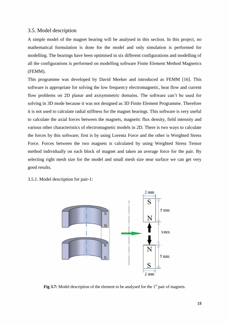
3.5.1. Model description for pair-1:
Fig 3.7: Model description of the element to be analysed for the 1st pair of magnets.
19
3.5.2. Model description for pair-2:
Fig 3.8: Model description of the element to be analysed for 2nd
pair of magnets.
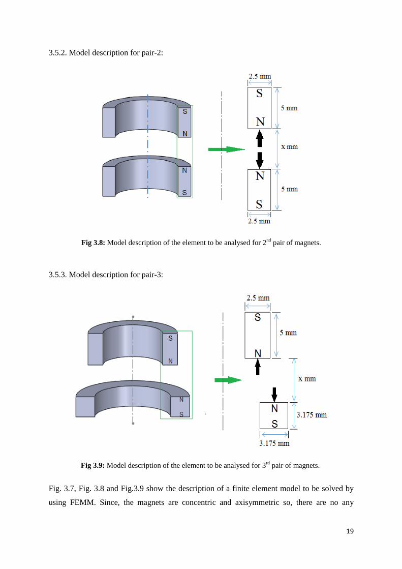
3.5.3. Model description for pair-3:
Fig 3.9: Model description of the element to be analysed for 3rd
pair of magnets.
Fig. 3.7, Fig. 3.8 and Fig.3.9 show the description of a finite element model to be solved by
using FEMM. Since, the magnets are concentric and axisymmetric so, there are no any
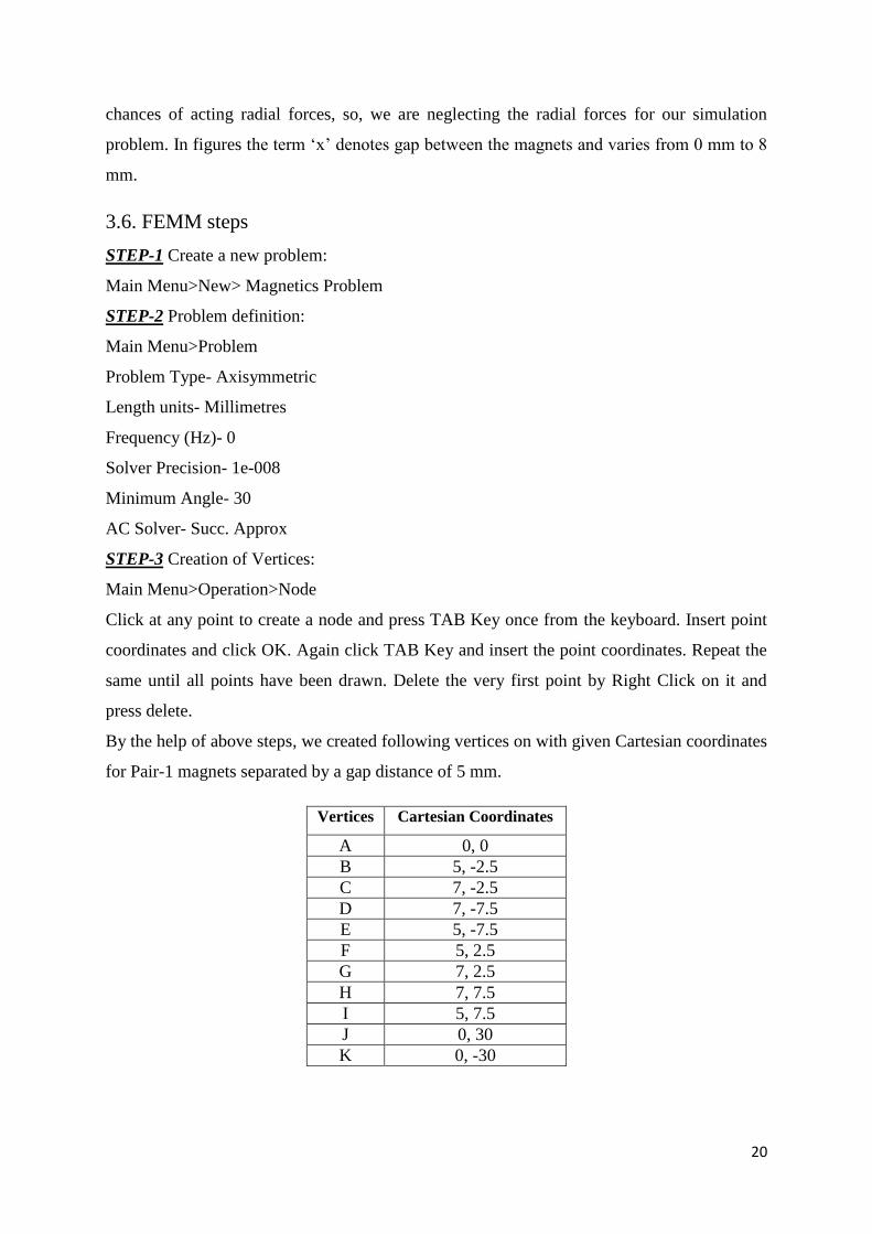
20
chances of acting radial forces, so, we are neglecting the radial forces for our simulation
problem. In figures the term ‗x‘ denotes gap between the magnets and varies from 0 mm to 8
mm.
3.6. FEMM steps
STEP-1 Create a new problem:
Main Menu>New> Magnetics Problem
STEP-2 Problem definition:
Main Menu>Problem
Problem Type- Axisymmetric
Length units- Millimetres
Frequency (Hz)- 0
Solver Precision- 1e-008
Minimum Angle- 30
AC Solver- Succ. Approx
STEP-3 Creation of Vertices:
Main Menu>Operation>Node
Click at any point to create a node and press TAB Key once from the keyboard. Insert point
coordinates and click OK. Again click TAB Key and insert the point coordinates. Repeat the
same until all points have been drawn. Delete the very first point by Right Click on it and
press delete.
By the help of above steps, we created following vertices on with given Cartesian coordinates
for Pair-1 magnets separated by a gap distance of 5 mm.
Vertices Cartesian Coordinates
A 0, 0
B 5, -2.5
C 7, -2.5
D 7, -7.5
E 5, -7.5
F 5, 2.5
G 7, 2.5
H 7, 7.5
I 5, 7.5
J 0, 30
K 0, -30

21
STEP-4 Creation of line:
Main Menu>Operation>Segment
Click on a vertices and click on another one. Repeat the process and select the other vertices
to create segments.
Create the lines by joining the Vertices as BC, CD, DE, EB, FG, GH, HI, IF, JK
STEP-5 Creation of Arc:
Main Menu>Operation>Arc Segment
Click on a vertices and click on another one to create an Arc as KJ. A window will open
> Arc Segment Properties
Arc Angle- 180
Max. Segment, Degrees- 1
Boundary cond. - <None>
STEP-6 Creation of Blocks:
Main menu>Operation>Block
Just create blocks by clicking inside the BCDE, FGHI and inside of Arc Segment KJ. In this
case three numbers of blocks is to be created.
STEP-7 Select Appropriate Material from Materials Library:
Main Menu>Properties> Materials Library
Library Materials- First click on Air. Drag and drop it to a Model Materials column at right.
Select an appropriate Material for other blocks. Drag and drop it too at right. In the current
case-
PM Materials>NdFeB Magnets>NdFeB 42 MGOe and click OK.
STEP-8 Define Materials:
In case when the particular material is not available in the Materials Library
Main Menu>Properties>Materials>Add Property
Then input the properties of that material with name
Name-
B-H Curve-
Linear Material Properties
Relative µx-
Relative µy-
Coercivity-
Electrical Conductivity-
22
Click OK.
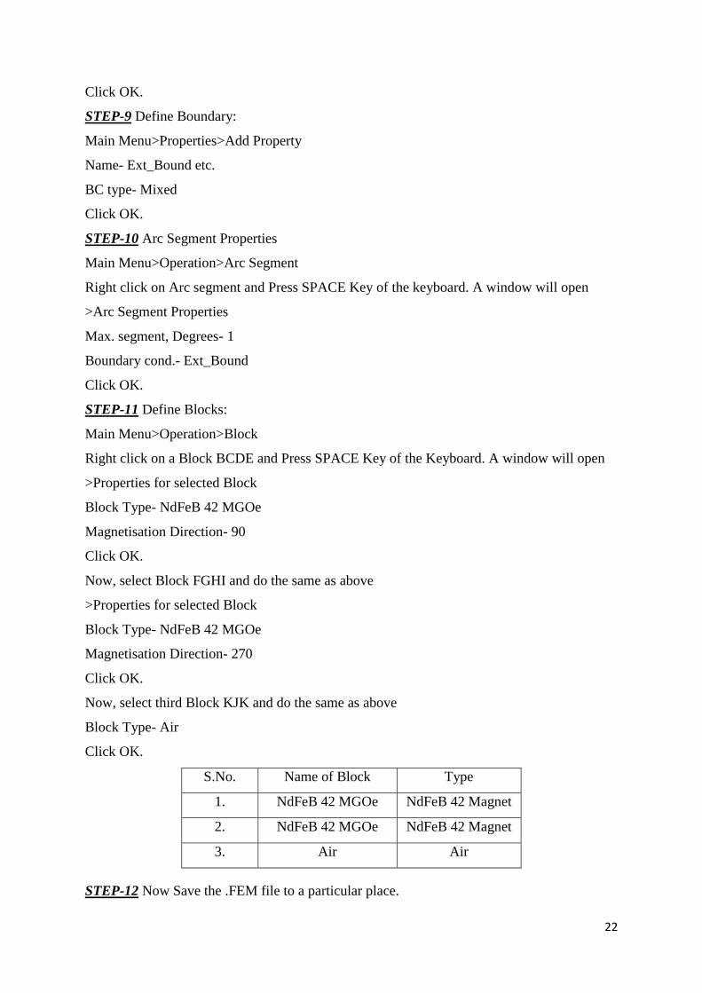
STEP-9 Define Boundary:
Main Menu>Properties>Add Property
Name- Ext_Bound etc.
BC type- Mixed
Click OK.
STEP-10 Arc Segment Properties
Main Menu>Operation>Arc Segment
Right click on Arc segment and Press SPACE Key of the keyboard. A window will open
>Arc Segment Properties
Max. segment, Degrees- 1
Boundary cond.- Ext_Bound
Click OK.
STEP-11 Define Blocks:
Main Menu>Operation>Block
Right click on a Block BCDE and Press SPACE Key of the Keyboard. A window will open
>Properties for selected Block
Block Type- NdFeB 42 MGOe
Magnetisation Direction- 90
Click OK.
Now, select Block FGHI and do the same as above
>Properties for selected Block
Block Type- NdFeB 42 MGOe
Magnetisation Direction- 270
Click OK.
Now, select third Block KJK and do the same as above
Block Type- Air
Click OK.
S.No. Name of Block Type
1. NdFeB 42 MGOe NdFeB 42 Magnet
2. NdFeB 42 MGOe NdFeB 42 Magnet
3. Air Air
STEP-12 Now Save the .FEM file to a particular place.

23
STEP-13 Create Mesh:
Main Menu>Mesh>Create Mesh
The mesh will be created.
(a) (b)
Fig 3.10: (a). Created mesh for 1st pair of N42 type magnets. (b). Closer view of mesh.
STEP-14 Run Analysis:
Main Menu>Analysis>Analyze>View Results
Fig 3.11: Magnetic Field lines for the pair of magnet after analysing.
24
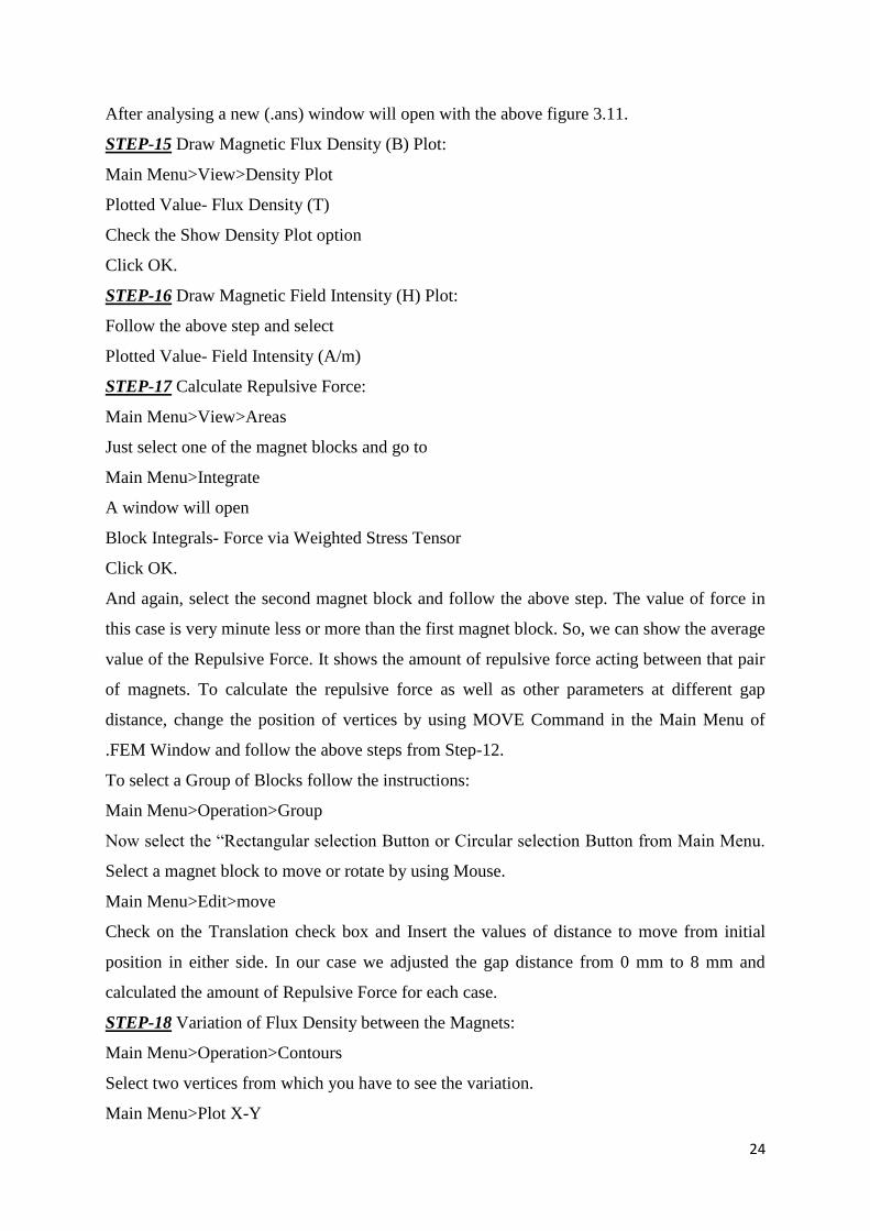
After analysing a new (.ans) window will open with the above figure 3.11.
STEP-15 Draw Magnetic Flux Density (B) Plot:
Main Menu>View>Density Plot
Plotted Value- Flux Density (T)
Check the Show Density Plot option
Click OK.
STEP-16 Draw Magnetic Field Intensity (H) Plot:
Follow the above step and select
Plotted Value- Field Intensity (A/m)
STEP-17 Calculate Repulsive Force:
Main Menu>View>Areas
Just select one of the magnet blocks and go to
Main Menu>Integrate
A window will open
Block Integrals- Force via Weighted Stress Tensor
Click OK.
And again, select the second magnet block and follow the above step. The value of force in
this case is very minute less or more than the first magnet block. So, we can show the average
value of the Repulsive Force. It shows the amount of repulsive force acting between that pair
of magnets. To calculate the repulsive force as well as other parameters at different gap
distance, change the position of vertices by using MOVE Command in the Main Menu of
.FEM Window and follow the above steps from Step-12.
To select a Group of Blocks follow the instructions:
Main Menu>Operation>Group
Now select the ―Rectangular selection Button or Circular selection Button from Main Menu.
Select a magnet block to move or rotate by using Mouse.
Main Menu>Edit>move
Check on the Translation check box and Insert the values of distance to move from initial
position in either side. In our case we adjusted the gap distance from 0 mm to 8 mm and
calculated the amount of Repulsive Force for each case.
STEP-18 Variation of Flux Density between the Magnets:
Main Menu>Operation>Contours
Select two vertices from which you have to see the variation.
Main Menu>Plot X-Y

25
Plot Type- |B| (Magnitude of flux density)
Number of points in plot- Insert any number of points
Check the Write data to text file check box, if you want to get the values in tabulation form.
Click OK.
It will show the values of Magnetic flux density at each point of that line.
STEP-19 Variation of Magnetic Field Intensity (H) between the magnets:
Follow the above step and choose
Plot Type- |H| (Magnitude of field Intensity).
STEP-20 Vector plot of Magnetic Flux Density and Field Intensity:
Main Menu>View>Vector Plot
Vector Plot Type- Select either B or H
Scaling Factor- Insert 1 or more
Click OK.
To calculate the above characteristics for the other pairs of N42 type magnets, just follow all
the above steps. To calculate the same for the pairs of N52 type magnets, also follow the
above steps except Step-7. Just do some changes in the details as follows:
STEP-7(For N52) Select Appropriate Material from Materials Library:
Main Menu>Properties> Materials Library
Library Materials- First click on Air. Drag and drop it to a Model Materials column at right.
Select an appropriate Material for other blocks. Drag and drop it too at right. In current case-
PM Materials>NdFeB Magnets>NdFeB 52 MGOe and click OK.

26
Chapter -4
Results and Discussion
In the Fig. 4.1, it is shown that as the coercive strength of the magnetic material increases, the
value of repulsive force also increases. For a particular grade of magnetic material, the value
of coercive strength, as well as operating temperature, remains unaffected with the variation
to the shape and size of the magnet. The below figure shows that as the gap between the two
magnets increases, the intensity of repulsive force decreases and when the gap between the
two magnets decreases, the value of repulsive force increases. The repulsive force is
maximum at a distance zero i.e. no gap between the magnets. The average value of coercive
strength is taken for N42 magnets, since; it varies between 9,15,000 A/m to 10,00,000 A/m
and the average value is 9,57,500 A/m. All the simulation for N42 type ring magnets is
performed by considering the coercive strength as 9,57,500 A/m. As the below graph shows,
the maximum value of magnetic repulsion force varies approximately between 38 N to 48 N
so, the mid-value of force, as well as related specifications, is considered for the modelling.
Fig 4.1: Repulsive force distribution for a N42 type ring magnet of dimension 15×10×5 mm and
15×10×5 mm at 3 different coercive strength values.
4.1. Repulsive force variation for N42 and N52 type of neodymium magnets
Fig. 4.2 shows the variation of repulsive force for the three configurations of the N42 type
permanent ring magnet. It is clear from the graph that greater the surface area of magnets
0
5
10
15
20
25
30
35
40
45
50
0 1 2 3 4 5 6 7 8 9
Rep
uls
ive
Forc
e(N
ewto
n)
Distance(mm)
Distance Vs Repulsive Force
Hc=915000 A/mHc=957500 A/mHc=1000000 A/m

27
facing each other, as well as the thickness of the magnets in the direction of magnetisation,
greater, will be the force of repulsion. The force of repulsion is maximum for pair-2 magnet
configurations as compared to other pairs.
Fig 4.2: Repulsive force variation for 3 different combinations of N42 type ring magnets.
Fig 4.3: Repulsive force variation for 3 different combinations of N52 type ring magnets.
0
5
10
15
20
25
30
35
40
45
0 1 2 3 4 5 6 7 8 9
Rep
uls
ive
Fo
ece(
New
ton
)
Distance(mm)
Distance Vs Repulsive Force
14x10x5 mm and 14x10x5 mm
15x10x5 mm and 15x10x5 mm
15x10x5 mm and19.05x12.7x3.175 mm
0
10
20
30
40
50
60
70
0 1 2 3 4 5 6 7 8 9
Rep
uls
ive
Forc
e(N
ewto
n)
Distance(mm)
Distance Vs Repulsive Force
14x10x5 mm and 14x10x5 mm
15x10x5 mm and 15x10x5 mm
15x10x5 mm and19.05x12.7x3.175 mm

28
Fig. 4.3 shows that the value of repulsive force for the second pair of magnets is much higher
than other pairs for a gap of less than 5 mm. It is clear from the graph that as the gap distance
increases the repulsive force strength decreases and about a distance of 8 mm all the pairs
shows an equal amount of repulsive force. Fig. 4.2 and Fig. 4.3 also shows that the value of
repulsive force is more for N52 magnets than that of N42 magnets for all three
configurations.
Table 4.1: Values of Repulsive force obtained for all pairs of magnets.
Distance
between
the
magnets,
(in mm)
Repulsive force acting between the magnets, (in Newton)
N42 type magnet N52 type magnet
Pair-1 Pair-2 Pair-3 Pair-1 Pair-2 Pair-3
0 35.5828 42.7638 8.49991 48.8915 58.6974 6.5592
0.5 20.3406 26.4249 8.35504 24.1313 30.8559 8.30656
1 13.4081 18.2791 7.701 16.6688 22.3013 8.94975
1.5 9.28972 13.5062 6.76867 11.885 16.9316 8.36613
2 6.95397 10.1107 5.82803 9.02119 13.9256 7.40412
2.5 5.18955 7.88378 5.12155 6.79888 10.1887 6.56901
3 4.07553 6.10376 4.39932 5.37332 7.959 5.72181
3.5 3.30084 5.08226 3.7232 4.36996 6.66411 4.85906
4 2.7101 4.23307 3.25344 3.60134 5.56894 4.26117
4.5 2.2631 3.52262 2.7886 3.01648 4.64938 3.66924
5 1.95334 3.04169 2.52921 2.60523 4.02785 3.33434
5.5 1.70631 2.64306 2.16239 2.28246 3.51001 2.85429
6 1.44046 2.31853 1.94965 1.92933 3.08405 2.58318
6.5 1.27065 2.08985 1.799 1.7041 2.77803 2.39063
7 1.11023 1.85008 1.56414 1.49042 2.4685 2.08154
7.5 1.02011 1.5932 1.40548 1.37319 2.13256 1.87218
8 0.932356 1.43214 1.30339 1.25422 1.91868 1.73517
4.2. Variation of magnetic flux density for a particular dimension of magnets
Fig. 4.4 shows the variation of magnetic flux density for second pair of N42 type permanent
magnet and the graph illustrates that the density of magnetic flux is more at the outer corners,
radius of 7.5 mm, of the ring magnets as compared to the density of magnetic flux at inner

29
corners i.e. at radius of 5 mm. The flux density is minimum at the middle of the facing
surfaces at a radius of 6.25 mm. The density also varies more between the middle of the gap
and it is maximum at outer corners, minimum at inner corners. From the graph, it is clear that
the variation of flux density is very low at a radius of 6.25 mm i.e. between the middle of the
edges of inner and outer corners. The variation of flux density is also shown by fig. 4.5, for a
N52 type of permanent ring magnet of same dimensions as in Fig. 4.4.
Table 4.2: Flux density variation data for ring magnets in straight lines having dimensions of
15×10×5 mm and 15×10×5 mm separated by a distance of 5 mm.
Distance
between the
magnets,
(in mm)
Magnetic flux density, B (in Tesla)
N42 type magnet N52 type magnet
r =5 mm r =6.25 mm r =7.25 mm r =5 mm r =6.25 mm r =7.25
mm
0.00E+00 1.18E+00 4.65E-01 1.24E+00 1.47E+00 4.95E-01 1.48E+00
5.56E-01 2.60E-01 3.14E-01 3.85E-01 2.92E-01 3.44E-01 4.34E-01
1.11E+00 1.39E-01 2.00E-01 2.58E-01 1.57E-01 2.23E-01 2.92E-01
1.67E+00 7.23E-02 1.38E-01 2.00E-01 8.20E-02 1.54E-01 2.26E-01
2.22E+00 3.44E-02 8.29E-02 1.74E-01 3.93E-02 9.27E-02 1.97E-01
2.78E+00 3.43E-02 8.47E-02 1.75E-01 3.92E-02 9.46E-02 1.98E-01
3.33E+00 7.45E-02 1.28E-01 1.99E-01 8.43E-02 1.43E-01 2.25E-01
3.89E+00 1.38E-01 2.05E-01 2.60E-01 1.55E-01 2.27E-01 2.94E-01
4.44E+00 2.59E-01 3.17E-01 3.79E-01 2.91E-01 3.47E-01 4.29E-01
5.00E+00 1.11E+00 4.67E-01 1.24E+00 1.33E+00 4.99E-01 1.47E+00
Fig 4.4: Flux density(B) variation for a N42 type ring magnets of dimensions 15×10×5 and
15×10×5 separated by a distance of 5 mm.
0.00E+00
2.00E-01
4.00E-01
6.00E-01
8.00E-01
1.00E+00
1.20E+00
1.40E+00
0.00E+00 1.00E+00 2.00E+00 3.00E+00 4.00E+00 5.00E+00 6.00E+00
Mag
net
ic f
lux
den
sity
,B (
Tes
la)
Distance (mm)
r=5 mm
r=6.25 mm
r=7.5 mm

30
The difference between the both models is that the density of magnetic flux is more for N52
type magnets than that of the N42 type magnets, near the surfaces, but the variation is about
equal at the middle of the gap at radius 6.25 mm.
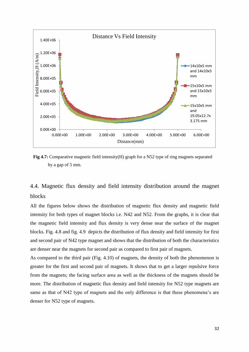
4.3. Variation of magnetic field intensity
The variation of magnetic field intensity has also been analysed between the magnets of both
types i.e. N42 and N52, for a gap of 5 mm between the magnets. In figure 4.6, it is shown that
the second pair of magnets possesses the maximum intensity of the magnetic field at their
surfaces. The variation of field intensity for the first pair and third pair of magnets are almost
equal and is closer to the variation for second pair. At near the middle of the gap, we can see
that the variation is more as compared to the near the surfaces.
Fig. 4.7 also depicts the variation of the intensity of magnetic field for N52 type magnet
pairs. The difference between the field intensity distribution for N42 type and N52 type of
magnets is that N52 type magnets possesses more field intensity near the faces, while field
intensity variation is nearly same at the middle of the ring magnets. This shows that the N52
type magnets are stronger than the same dimensions of the N42 type magnets.
Fig 4.5: Flux density(B) variation for a N52 type ring magnets of dimensions 15×10×5 and
15×10×5 separated by a distance of 5 mm.
0.00E+00
2.00E-01
4.00E-01
6.00E-01
8.00E-01
1.00E+00
1.20E+00
1.40E+00
1.60E+00
0.00E+00 1.00E+00 2.00E+00 3.00E+00 4.00E+00 5.00E+00 6.00E+00
Mag
net
ic f
lux
den
sity
, B
(T
esla
)
Distance (mm)
r=5 mm
r=6.25 mm
r= 7.5 mm

31
Table 4.3: Data obtained for variation of magnetic field intensity along the lines joining the
outer diameter of each magnetic pair at a gap of 5 mm.
Distance between
the magnets,
(in mm)
Magnetic field intensity, H (in A/m)
N42 type magnet N52 type magnet
Pair-1 Pair-2 Pair-3 Pair-1 Pair-2 Pair-3
0.00E+00 9.35E+05 9.84E+05 9.30E+05 1.13E+06 1.17E+06 1.11E+06
5.05E-01 2.86E+05 3.22E+05 2.75E+05 3.24E+05 3.63E+05 3.13E+05
1.01E+00 1.91E+05 2.18E+05 1.81E+05 2.17E+05 2.47E+05 2.07E+05
1.52E+00 1.40E+05 1.69E+05 1.41E+05 1.59E+05 1.91E+05 1.60E+05
2.02E+00 1.14E+05 1.43E+05 1.23E+05 1.30E+05 1.62E+05 1.39E+05
2.53E+00 1.07E+05 1.34E+05 1.24E+05 1.21E+05 1.51E+05 1.40E+05
3.03E+00 1.18E+05 1.46E+05 1.41E+05 1.35E+05 1.66E+05 1.59E+05
3.48E+00 1.39E+05 1.70E+05 1.70E+05 1.58E+05 1.92E+05 1.91E+05
3.99E+00 1.86E+05 2.20E+05 2.17E+05 2.12E+05 2.48E+05 2.43E+05
4.49E+00 2.91E+05 3.15E+05 3.17E+05 3.30E+05 3.56E+05 3.54E+05
5.00E+00 9.52E+05 9.84E+05 9.51E+05 1.14E+06 1.17E+06 1.14E+06
Fig 4.6: Comparative magnetic field intensity(H) graph for a N42 type of ring magnets separated
by a gap of 5 mm.
0.00E+00
2.00E+05
4.00E+05
6.00E+05
8.00E+05
1.00E+06
1.20E+06
0.00E+00 1.00E+00 2.00E+00 3.00E+00 4.00E+00 5.00E+00 6.00E+00
Fie
ld I
nte
nsi
ty,H
(A
/m)
Distance(mm)
Distance Vs Field Intensity
14x10x5 mmand 14x10x5mm
15x10x5 mmand 15x10x5mm
15x10x5 mmand19.05x12.7x3.175 mm
32
Fig 4.7: Comparative magnetic field intensity(H) graph for a N52 type of ring magnets separated
by a gap of 5 mm.
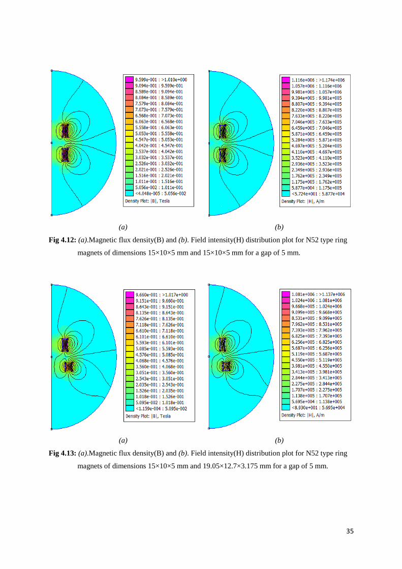
4.4. Magnetic flux density and field intensity distribution around the magnet
blocks
All the figures below shows the distribution of magnetic flux density and magnetic field
intensity for both types of magnet blocks i.e. N42 and N52. From the graphs, it is clear that
the magnetic field intensity and flux density is very dense near the surface of the magnet
blocks. Fig. 4.8 and fig. 4.9 depicts the distribution of flux density and field intensity for first
and second pair of N42 type magnet and shows that the distribution of both the characteristics
are denser near the magnets for second pair as compared to first pair of magnets.
As compared to the third pair (Fig. 4.10) of magnets, the density of both the phenomenon is
greater for the first and second pair of magnets. It shows that to get a larger repulsive force
from the magnets; the facing surface area as well as the thickness of the magnets should be
more. The distribution of magnetic flux density and field intensity for N52 type magnets are
same as that of N42 type of magnets and the only difference is that these phenomena‘s are
denser for N52 type of magnets.
0.00E+00
2.00E+05
4.00E+05
6.00E+05
8.00E+05
1.00E+06
1.20E+06
1.40E+06
0.00E+00 1.00E+00 2.00E+00 3.00E+00 4.00E+00 5.00E+00 6.00E+00
Fie
ld I
nte
nsi
ty,H
(A
/m)
Distance(mm)
Distance Vs Field Intensity
14x10x5 mmand 14x10x5mm
15x10x5 mmand 15x10x5mm
15x10x5 mmand19.05x12.7x3.175 mm

33
(a) (b)
Fig 4.8: (a).Magnetic flux density(B) and (b). Field intensity(H) distribution plot for N42 type ring
magnets of dimensions 14×10×5 mm and 14×10×5 mm for a gap of 5 mm.
(a) (b)
Fig 4.9: (a).Magnetic flux density(B) and (b). Field intensity(H) distribution plot for N42 type ring
magnets of dimensions 15×10×5 mm and 15×10×5 mm for a gap of 5 mm.

34
(a) (b)
Fig 4.10: (a).Magnetic flux density(B) and (b). Field intensity(H) distribution plot for N42 type ring
magnets of dimensions 15×10×5 mm and 19.05×12.7×3.175 mm for a gap of 5 mm.
(a) (b)
Fig 4.11: (a).Magnetic flux density(B) and (b). Field intensity(H) distribution plot for N52 type ring
magnets of dimensions 14×10×5 mm and 14×10×5 mm for a gap of 5 mm.
35
(a) (b)
Fig 4.12: (a).Magnetic flux density(B) and (b). Field intensity(H) distribution plot for N52 type ring
magnets of dimensions 15×10×5 mm and 15×10×5 mm for a gap of 5 mm.
(a) (b)
Fig 4.13: (a).Magnetic flux density(B) and (b). Field intensity(H) distribution plot for N52 type ring
magnets of dimensions 15×10×5 mm and 19.05×12.7×3.175 mm for a gap of 5 mm.

36
Chapter -5
Conclusions
5.1. Conclusions
The simulation of the passive magnet bearing is performed to obtain an efficient way to
levitate the rotor of the turboexpander. This project is performed to find out a strong magnet
bearing which can suspend the rotor contactless at small clearances as well as can withstand
up to a certain temperature without losing its magnetic property. From the result section it is
observed that to achieve a greater repulsive force from any magnet pair, surface area of the
magnets, facing each other, thickness and type of magnetic material are the key factors.
The result shows that Neodymium (NdFeB) alloy magnet of grade N42 exert lower repulsive
force as compared to the grade N52 for the equal gap and dimensions. It is also important to
know that N52 has lower operating temperature (70oC) as compared to N42 (80
oC). So
according to the operating conditions any of the above grade of magnets can be used as
passive magnet bearing. For the current research work, it is suggested that magnets of grade
either N42 or N52, which is having dimensions of 15mm×10mm×5mm for each magnet can
be used for the suspension of rotor of the turboexpander. This is due to its more suspension
property as compared to other magnetic pairs.
5.2. Scope for future work
In present research work modelling of the passive magnet bearing by using modelling
software Finite Element Method Magnetics (FEMM) is performed, considering the problem
as a static problem. Modelling of the same bearing can be performed by considering it as a
dynamic problem i.e. the lower magnet remains static and the upper magnet bearing is in
motion. Experiments can also be performed on the magnet bearings in static as well as in
dynamic conditions and the experimental value can be compared with the value calculated
from simulation modelling.
37
References
1. Hirai, H., Hirokawa, M., Yoshida, S., Kamioka, Y., Takaike, A., Hayashi, H., and
Shiohara, Y. (2010). Development of a Neon Cryogenic turbo‐expander with
Magnetic Bearings. In Transactions of the Cryogenic Engineering Conference—CEC:
Advances in Cryogenic Engineering, 1218(1), 895-902.
2. Han, B., Liu, X., and Zheng, S. (2014). A Novel Integral 5-DOFs Hybrid Magnetic
Bearing with One Permanent Magnet Ring Used for Turboexpander. Mathematical
Problems in Engineering, 2014(162561).
3. Werner, P. (1978). "Self-pressurizing floating gas bearing having a magnetic bearing
therein." U.S. Patent No. 4,128,280.
4. Moser, R., Sandtner, J., and Bleuler, H. (2006). Optimization of repulsive passive
magnetic bearings. IEEE Transactions on Magnetics, 42(8), 2038-2042.
5. Falkowski, K., and Henzel, M. (2010). High efficiency radial passive magnetic
bearing. Solid State Phenomena, 164, 360-365.
6. Bekinal, S. I., Anil, T. R. R., Jana, S., Kulkarni, S. S., Sawant, A., Patil, N., and
Dhond, S. (2013). Permanent magnet thrust bearing: theoretical and experimental
results. Progress in Electromagnetics Research B, 56, 269-287.
7. Kumbernuss, J., Jian, C., Wang, J., Yang, H. X., and Fu, W. N. (2012). A novel
magnetic levitated bearing system for Vertical Axis Wind Turbines (VAWT). Applied
Energy, 90(1), 148-153.
8. Kuroki, J., Shinshi, T., Li, L., and Shimokohbe, A. (2005). Miniaturization of a one-
axis-controlled magnetic bearing. Precision Engineering, 29(2), 208-218.
9. Jinji, S., Yuan, R., and Jiancheng, F. (2011). Passive axial magnetic bearing with
Halbach magnetized array in magnetically suspended control moment gyro
application. Journal of Magnetism and Magnetic Materials, 323(15), 2103-2107.
10. http://www.rare-earth-magnets.com/history-of-magnetism-and-electricity/ (2015).
11. Faus, H. T. (1943). "Magnetic suspension." U.S. Patent No. 2,315,408.
12. Mendelsohn, L. I. (1953). "Repulsion type magnetic suspension." U.S. Patent No.
2,658,805.
13. Rava, E. (1976). "Radial magnetic bearing." U.S. Patent No. 3,954,310.
14. Timmerman, J. (1957). "Anisotropic permanent magnetic cylindrical member." U.S.
Patent No. 2,803,765.
15. Baermann, M. (1966). "Permanent magnetic bearing." U.S. Patent No. 3,233,950.

38
16. Meeker, D. "FEMM - Finite Element Method Magnetics", http://femm.foster-
miller.net. (2015).
17. http://www.amazingmagnets.com/magnetgrades.aspx (2015).
18. Granström, M. (2011). "Design och Analys av ettmagnetlager med 1-frihetsgrad."
19. Hamler, A., Gorican, V., Štumberger, B., Jesenik, M., and Trlep, M. (2004). Passive
magnetic bearing. Journal of magnetism and magnetic materials, 272, 2379-2380.
20. Ghosh, P. (2002). Analytical and Experimental Studies on Cryogenic Turboexpander.
A PhD. Thesis, Cryogenic Engineering Centre, IIT Kharagpur.
21. Samanta, P., and Hirani, H. (2008). Magnetic bearing configurations: Theoretical and
experimental studies. IEEE Transactions on Magnetics, 44(2), 292-300.
22. Ravaud, R., Lemarquand, G., and Lemarquand, V. (2009). Force and stiffness of
passive magnetic bearings using permanent magnets. Part 2: Radial magnetization.
IEEE Transactions on Magnetics, 45(9), 3334-3342.