Design of an experimental device for the … · POLITECNICO DI MILANO Scuola di Ingegneria...
110
POLITECNICO DI MILANO Scuola di Ingegneria Industriale Master of Science in Space Engineering DESIGN OF AN EXPERIMENTAL DEVICE FOR THE CHARACTERIZATION OF SOLAR CELLS IN LILT ENVIRONMENTS Relatore: Prof. Franco Bernelli Correlatore: Ing. Francesco Topputo Thesis by: Gioele ZGRAGGEN Matr. n. 754829 Academic Year 2012-2013
Transcript of Design of an experimental device for the … · POLITECNICO DI MILANO Scuola di Ingegneria...

POLITECNICO DI MILANOScuola di Ingegneria Industriale
Master of Science inSpace Engineering
DESIGN OF AN EXPERIMENTAL
DEVICE FOR THE CHARACTERIZATION
OF SOLAR CELLS IN LILT
ENVIRONMENTS
Relatore: Prof. Franco BernelliCorrelatore: Ing. Francesco Topputo
Thesis by:
Gioele ZGRAGGENMatr. n. 754829
Academic Year 2012-2013


”The best way to learn to flya spacecraft is to fly one.”
Wild Andy


Ringraziamenti
Vorrei innanzitutto ringraziare l’Ing. Francesco Topputo, per avermi datola disponibilita di lavorare a questa tesi, ma soprattutto per avermi seguitoin ogni momento, grazie ad i suoi insegnamenti ho imparato molto durantel’arco di questa tesi. Diverse persone sono state fondamentali per il lavorosvolto e senza di esse non sarei riuscito a svolgere tutto il lavoro: l’Ing.Giuseppe D’Amore, grazie alle sue conoscenze in elettrotecnica mi ha aiutatonella realizzazione della scheda elettronica, cosı come l’Ing. Alberto Dolara,l’Ing. Mauro Massari, grazie alle sue conoscenze ed alla sua disponibilita sonoriuscito a risolvere diversi problemi, l’Ing. Silvio Ferragina e l’Ing. MauroStrada per la realizzazione della serpentina di raffreddamento, l’Ing. MariaRosaria Pagano, l’Ing. Paolo Rubini e l’Ing. Alessandro Mattironi per iconsigli e gli aiuti nelle varie prove in laboratorio, infine il mio vicino di tesiAndrea Binci.Oltre a loro voglio ringraziare tutta la mia famiglia e i miei amici che mi sonsempre stati vicini in tutti questi anni.


Abstract
On March 2, 2004 at 07:17 UT the Rosetta Mission left from Kourou onthe Ariane 5 G+ launcher with the aim to arrive in 2014 on the comet67P/Churyumov-Gerasimenko. After reaching the comet, Rosetta will re-lease its lander Philae that will land on the comet. Its nominal life is guar-anteed by non-rechargeable primary batteries for a period of five comet days;further extension of the mission may be provided by six solar panels on thefaces of the lander Philae.The first purpose of this thesis is to create an environment similar to thatof the comet, mainly consisting in low temperatures (around -100°C) andlow solar intensity (0.11 Solar Constant); such conditions allows us study thebehaviour of the solar cells in both beginning and end of life (BOL, EOL).Indeed, for the EOL case, such test has never been performed before. For thisreason it has been built an experimental apparatus so as to be able to per-form the tests in these conditions and to store all the data into a computingenvironment.
Keywords:Solar cells; Low Intensity Low Temperature; Characterization I-V curve;Experimental device; Philae; Rosetta mission.
i

Sommario
Il 2 Marzo 2004 alle 07:17 UT e partita da Kourou con il lanciatore Ariane5 G+ la missione Rosetta con lo scopo di arrivare nel 2014 sulla cometa67P/Churyumov-Gerasimenko. Dopo aver raggiunto la cometa, Rosettasgancera il suo lander Philae che atterrera sulla cometa. La durata nom-inale di questa fase e di 5 giorni ed e garantita da batterie primarie nonricaricabili, un’ ulteriore prolungamento della missione puo essere reso pos-sibile da sei pannelli fotovoltaici presenti sulla facce di Philae.Lo scopo di questa tesi e di ricreare un ambiente simile a quello della cometa,ossia a basse temperature (attorno ai -100°C) e bassa intensita solare (0.11Solar Constant). Tali condizioni sono infatti necessarie per studiare il com-portamento delle celle solari a inizio vita (BOL) e fine vita (EOL), dato cheper il secondo caso non sono mai stati effettuati dei test. Per questo motivosi e costruito un apparato sperimentale in modo tale da poter effettuare delleprove in tali condizioni e elaborare tutti i dati direttamente al calcolatore.
Parole chiave:Celle solari; Bassa intensita bassa temperatura; Caratterizzazione curvaI-V; Apparato sperimentale; Philae; Missione Rosetta.
ii

Contents
Estratto in italiano xi
1 Introduction 1
2 Photovoltaic effect 32.1 Solar intensity . . . . . . . . . . . . . . . . . . . . . . . . . . . 32.2 Semiconductor materials . . . . . . . . . . . . . . . . . . . . . 42.3 Photovoltaic principle . . . . . . . . . . . . . . . . . . . . . . . 62.4 Characteristic of solar cells . . . . . . . . . . . . . . . . . . . . 62.5 Single junction silicon solar cells . . . . . . . . . . . . . . . . . 102.6 III-V solar cells . . . . . . . . . . . . . . . . . . . . . . . . . . 102.7 Temperature effects . . . . . . . . . . . . . . . . . . . . . . . . 11
2.7.1 Energy-gap . . . . . . . . . . . . . . . . . . . . . . . . 112.7.2 Carrier mobility . . . . . . . . . . . . . . . . . . . . . . 122.7.3 Dark currents and lifetimes . . . . . . . . . . . . . . . 13
2.8 Solar intensity effect . . . . . . . . . . . . . . . . . . . . . . . 132.9 Possible causes of performance loss in LILT conditions . . . . 142.10 Radiation damage . . . . . . . . . . . . . . . . . . . . . . . . . 15
2.10.1 Ionization . . . . . . . . . . . . . . . . . . . . . . . . . 152.10.2 Atomic displacements . . . . . . . . . . . . . . . . . . . 162.10.3 Electron displacement damage . . . . . . . . . . . . . . 162.10.4 Proton displacement damage . . . . . . . . . . . . . . . 172.10.5 Neutron displacement damage . . . . . . . . . . . . . . 17
3 Rosetta mission 183.1 Mission analysis . . . . . . . . . . . . . . . . . . . . . . . . . . 193.2 The comet . . . . . . . . . . . . . . . . . . . . . . . . . . . . . 23
3.2.1 What is a comet . . . . . . . . . . . . . . . . . . . . . 233.2.2 Characteristics of 67P/CG . . . . . . . . . . . . . . . . 233.2.3 The nucleus . . . . . . . . . . . . . . . . . . . . . . . . 253.2.4 Study of the comet . . . . . . . . . . . . . . . . . . . . 26
iii

Contents
3.2.5 Radiation on the comet . . . . . . . . . . . . . . . . . 263.2.6 Dimensions and shape . . . . . . . . . . . . . . . . . . 273.2.7 Axis of rotation . . . . . . . . . . . . . . . . . . . . . . 303.2.8 Shadow in a crater . . . . . . . . . . . . . . . . . . . . 303.2.9 Gas production . . . . . . . . . . . . . . . . . . . . . . 313.2.10 Dust production . . . . . . . . . . . . . . . . . . . . . . 333.2.11 Dynamics of comet dust . . . . . . . . . . . . . . . . . 363.2.12 Optical opacity due to dust . . . . . . . . . . . . . . . 393.2.13 Lighting conditions . . . . . . . . . . . . . . . . . . . . 40
3.3 The spacecraft . . . . . . . . . . . . . . . . . . . . . . . . . . . 423.4 The lander Philae . . . . . . . . . . . . . . . . . . . . . . . . . 44
3.4.1 Philae design . . . . . . . . . . . . . . . . . . . . . . . 473.4.2 Philae Power SubSystem . . . . . . . . . . . . . . . . . 473.4.3 Solar arrays design . . . . . . . . . . . . . . . . . . . . 483.4.4 General description of the solar cells . . . . . . . . . . 503.4.5 Output power . . . . . . . . . . . . . . . . . . . . . . . 513.4.6 Variation due to Solar Constant . . . . . . . . . . . . . 523.4.7 Degradation due to Radiation . . . . . . . . . . . . . . 523.4.8 Variation due to temperature . . . . . . . . . . . . . . 533.4.9 Variation with incidence angle . . . . . . . . . . . . . . 53
4 Design of the experimental apparatus for LILT measure-ments 544.1 Base plate and cooling coil . . . . . . . . . . . . . . . . . . . . 544.2 Electronic board . . . . . . . . . . . . . . . . . . . . . . . . . 56
4.2.1 Deriving the equations of a charging capacitor by PVgenerator . . . . . . . . . . . . . . . . . . . . . . . . . 57
4.2.2 Description of the board . . . . . . . . . . . . . . . . . 614.2.3 Software for data acquisition . . . . . . . . . . . . . . . 654.2.4 Characterization of the operational amplifier . . . . . . 66
5 Tests 745.1 State of test . . . . . . . . . . . . . . . . . . . . . . . . . . . . 74
5.1.1 Tests carried out . . . . . . . . . . . . . . . . . . . . . 745.1.2 Alenia report . . . . . . . . . . . . . . . . . . . . . . . 745.1.3 Test made by Politecnico di Milano . . . . . . . . . . . 755.1.4 Test made by INTA . . . . . . . . . . . . . . . . . . . . 755.1.5 Tests to be made . . . . . . . . . . . . . . . . . . . . . 75
5.2 Dark current characterisation . . . . . . . . . . . . . . . . . . 765.2.1 Experiment on Philae solar cell . . . . . . . . . . . . . 765.2.2 Experiment made at Polimi . . . . . . . . . . . . . . . 78
iv

Contents
5.2.3 Consideration . . . . . . . . . . . . . . . . . . . . . . . 805.3 Laboratory conditions test . . . . . . . . . . . . . . . . . . . . 80
6 Conclusions 846.1 Future developments . . . . . . . . . . . . . . . . . . . . . . . 85
List of acronyms and abbreviations 86
Bibliography 87
v

List of Figures
1.1 Graphic representation of the LILT area [1]. . . . . . . . . . . 2
2.1 Spectrum of the radiation outside the Earth’s atmospherecompared to spectrum of a 5800 K blackbody. . . . . . . . . . 4
2.2 Diagram of the two-dimensional covalent bonds between thesilicon atoms [15]. . . . . . . . . . . . . . . . . . . . . . . . . . 5
2.3 Silicon drugged with boron and phosphorus, which generatesfree charge carriers, that are positive (holes) or negative (elec-trons) [15]. . . . . . . . . . . . . . . . . . . . . . . . . . . . . . 6
2.4 Simplified diagram of a solar cell in which are depicted thebasic elements [15]. . . . . . . . . . . . . . . . . . . . . . . . . 7
2.5 (a)Example of I-V curve of a solar cell illuminated. (b) Exam-ple of I-V curve in accordance with the generator convention[15]. . . . . . . . . . . . . . . . . . . . . . . . . . . . . . . . . 8
2.6 Conventional solar cell model with photo current IL, diodecurrent I0, shunt resistance Rsh, series resistance Rs, outputvoltage V , output current I and load resistance RL [29]. . . . 9
2.7 Energy that can be used by a silicon solar cell. . . . . . . . . . 10
2.8 Energy that can be used by a triple junction solar cell. . . . . 11
2.9 Typical LILT degradation phenomena can become apparentunder LILT measurement conditions.[19] . . . . . . . . . . . . 14
3.1 Graphical representation of the orbit of Rosetta [3]. . . . . . . 20
3.2 Trend of the distance between Rosetta and the Sun, and thelight intensity [1]. . . . . . . . . . . . . . . . . . . . . . . . . . 21
3.3 Trend of the solar intensity in W/m2 on Rosetta spacecraftduring all the mission time [1]. . . . . . . . . . . . . . . . . . . 22
3.4 Trend of the solar intensity in SC for the period of operationof Philae on the comet [1]. . . . . . . . . . . . . . . . . . . . . 22
3.5 Discovery image of comet 67P/Churyumov–Gerasimenko in1969 [9]. . . . . . . . . . . . . . . . . . . . . . . . . . . . . . . 24
vi

List of Figures
3.6 The prograde (top row) and the retrograde (bottom row) so-lutions for the threedimensional shape of the nucleus of comet67P/CG reconstructed from the inversion of the 2003 HSTand 2005 NTT light curves. For each solution, three viewsof the reconstructed 3-D shape model are displayed at threedifferent rotational phase angles: 350°, 80°, and pole-on viewof the 80° model [33]. . . . . . . . . . . . . . . . . . . . . . . . 28
3.7 Light curves from HST and NNT. The dots represent therecorded data and lines the best-fit for the two solutions [9]. . 29
3.8 Constraints on the direction of the rotational axis of the nu-cleus of comet 67P/Churyumov-Gerasimenko as determinedby different authors [9]. . . . . . . . . . . . . . . . . . . . . . . 31
3.9 Observed gas production rates versus time from perihelion forComet 67P/Churyumov–Gerasimenko [9]. . . . . . . . . . . . 32
3.10 Solid line: phase function of an individual dust particle asgiven in Divine (1981), but here normalised to j(α = 0) = 1.Dashed line: geometric phase function jgeo(α) Muller (1999)[13]. . . . . . . . . . . . . . . . . . . . . . . . . . . . . . . . . 34
3.11 Observed Afρ values as function of heliocentric distance rh [13]. 35
3.12 Observed Afρ values corrected for phase angle through divi-sion by the geometric phase function and power law fit forphase-angle-corrected [13]. . . . . . . . . . . . . . . . . . . . . 35
3.13 Measured H2O production rates with corresponding power law[13]. . . . . . . . . . . . . . . . . . . . . . . . . . . . . . . . . 36
3.14 Synchrones are shown projected in the comet orbit plane (left)and image plane (right). The solid lines correspond to syn-chrones for different period of times, the dashed lines corre-spond to syndynes for different values of β [13]. . . . . . . . . 37
3.15 Number fraction over particle radius for the three differentialsize distributions [13]. . . . . . . . . . . . . . . . . . . . . . . . 38
3.16 Trend of the value of Afτ and τ as a function of distance fromthe Sun [1] . . . . . . . . . . . . . . . . . . . . . . . . . . . . . 39
3.17 Performance of the light intensity with and without τ as afunction of distance from the Sun [1]. . . . . . . . . . . . . . . 40
3.18 Light intensity of the soil of the comet as a function of the daysat perihelion. Are indicated respectively, the day of the landerlanding, the spring equinox, the perihelion and the nominalend of mission, 31/12/2015 [1]. . . . . . . . . . . . . . . . . . . 41
3.19 Light intensity on a horizontal panel during the first 10-daymission at the equator [1]. . . . . . . . . . . . . . . . . . . . . 41
vii

List of Figures
3.20 Vector Sun at intervals of one hour for a landing probe onthe equator, from the first day of the mission to the comet’sperihelion [1]. . . . . . . . . . . . . . . . . . . . . . . . . . . . 42
3.21 The Rosetta spacecraft and its scientific payload [3]. . . . . . . 44
3.22 Rosetta Lander, Philae, in landed configuration [32]. . . . . . . 45
3.23 Philae landing scenario [30]. . . . . . . . . . . . . . . . . . . . 45
3.24 Philae solar array [29]. . . . . . . . . . . . . . . . . . . . . . . 49
3.25 Conventional solar cell I-V curve in 3 quadrants. In quadrantI, power is produced; in quadrant II, the cell is reverse-biased[29]. . . . . . . . . . . . . . . . . . . . . . . . . . . . . . . . . 51
4.1 Internal vista of half (coil made with Autodesk Inventor). . . . 55
4.2 External vista of half coil (made with Autodesk Inventor). . . 55
4.3 Image of the copper coil. . . . . . . . . . . . . . . . . . . . . . 56
4.4 Test on the aluminium coil at low temperature with liquidnitrogen. . . . . . . . . . . . . . . . . . . . . . . . . . . . . . . 57
4.5 Equivalent circuit of a PV cell, module or array (PV generator)with a capacitor as load. . . . . . . . . . . . . . . . . . . . . . 57
4.6 Pictures of the first part of the electronic board. . . . . . . . . 61
4.7 Pictures of the second part of the electronic board. . . . . . . 62
4.8 Sketch of the scheme of the electronic board. . . . . . . . . . . 64
4.9 Sketch of the two operational amplifier for the current. . . . . 64
4.10 Pictures of the experimental apparatus in laboratory for test-ing the electronic board. . . . . . . . . . . . . . . . . . . . . . 66
4.11 Blocks in Simulink file for the management of the relays of theelectronic board. . . . . . . . . . . . . . . . . . . . . . . . . . 67
4.12 Blocks in Simulink file for the acquisition of the values of volt-age and current. . . . . . . . . . . . . . . . . . . . . . . . . . . 67
4.13 Graph of the current in mA and respective gain, G1 is withonly one operational amplifier, G2 with two operational am-plifier, in both cases the theoretical gain must be 706. . . . . . 73
5.1 Terminal I–V characteristics under full, partial, and zero illu-minations. . . . . . . . . . . . . . . . . . . . . . . . . . . . . . 78
5.2 Reverse (dark) I-V characteristics for different temperaturespresent in LUM. Irev in mA, Urev in V [29]. . . . . . . . . . . 78
5.3 Reverse (dark) I-V characteristics for different temperaturesin thermal vacuum chamber at the Polimi. I in mA, V in V. . 79
5.4 The cell in the thermal vacuum chamber. . . . . . . . . . . . . 80
5.5 Voltage in function of time for the test made on a cell atambient conditions. . . . . . . . . . . . . . . . . . . . . . . . . 81
viii

List of Figures
5.6 Current in function of time for the test made on a cell atambient conditions. . . . . . . . . . . . . . . . . . . . . . . . . 82
5.7 Curve I-V for the test made on a cell at ambient conditions inthe values of scale of the usb device. . . . . . . . . . . . . . . . 82
5.8 Curve I-V for the test made on a cell at ambient conditions. . 83
ix

List of Tables
2.1 Energy gap parameters for the two equations. . . . . . . . . . 122.2 Typical values of cross section dislocation in the silicon . . . . 17
3.1 The mission falls into several distinct phases [3]. . . . . . . . . 213.2 Minimum and maximum solar intensity during the Philae pe-
riod on the comet. . . . . . . . . . . . . . . . . . . . . . . . . 233.3 Comet 67P/CG parameters [6]. . . . . . . . . . . . . . . . . . 253.4 Principal physical parameters for the comet 67P/CG. . . . . . 293.5 Measurements of production rates by various authors. . . . . . 323.6 Values of α and γ found in the literature. . . . . . . . . . . . . 383.7 Number of strings and cells per module . . . . . . . . . . . . . 493.8 The Kelly cosine values of the photocurrent in silicon cells [23] 53
4.1 List of components used for the electronic board. . . . . . . . 634.2 Resistances that can be inserted in the second amplifier of the
current and respective gain of the operational amplifier. . . . . 654.3 Calculation of the gain for the voltage with the operational
amplifier “A”, the theoretical gain is 5. . . . . . . . . . . . . . 694.4 Calculation of the gain for the voltage with the operational
amplifier “E”, the theoretical gain is 5. . . . . . . . . . . . . . 704.5 Calculation of the gain for the current with two operational
amplifier insert, the first with a theoretical gain of 706, thesecond a theoretical gain of 1. . . . . . . . . . . . . . . . . . . 71
4.6 Calculation of the gain for the current with only one opera-tional amplifier insert, with a theoretical gain of 706. . . . . . 72
5.1 Characteristics of the tests made on the orbiter and on thelander of Rosetta at INTA . . . . . . . . . . . . . . . . . . . . 76
5.2 Summarizing table of the documents . . . . . . . . . . . . . . 77
x
Estratto in italiano
Progettazione di un apparato sperimentale per
la caratterizzazione di celle solari in ambiente
LILT
In queste pagine vengono ripresi i principali temi che sono trattati all’internodella tesi, lo scopo di essa era andare a costruire un apparato sperimentalein grado di caratterizzare le celle solari del lander Philae.
L’effetto fotovoltaico Il principio di funzionamento delle celle solari e laconversione fotovoltaica, che converte l’energia della luce direttamente in en-ergia elettrica.Le celle solari sono essenzialmente costituite da strati di materiale semicon-duttore con caratteristiche diverse. I principali materiali semiconduttori diinteresse per questo tipo di applicazione sono solidi cristallini, costituiti daelementi della IV colonna della tavola periodica di Mendelejev (silicio e ger-manio), o composti binari costituiti da elementi della III e V colonna (adesempio arseniuro di gallio, GaAs). L’effetto fotovoltaico e la creazione ditensione o di corrente elettrica in un materiale per esposizione alla luce.Quando la luce del sole o di qualsiasi altra luce e incidente su di una super-ficie di materiale, gli elettroni presenti nella banda di valenza di un atomometallico assorbono l’energia e, essendo eccitato, saltano alla banda di con-duzione e diventano liberi. Ora questi elettroni liberi sono attratti da unelettrodo caricato positivamente e quindi il circuito si completa e l’energiadella luce viene convertita in energia elettrica.
La missione rosetta E una missione dell’agnzia spaziale europea ESA,sviluppata a partire dagli anni ’90 con l’obbiettivo di atterrare e campionareil nucleo di una cometa. Rosetta e stata lanciata nel 2004 con lo scopo di rag-giungere la cometa 67P/Churyumov-Gerasimenko nel 2014 ad una distanzadi 3 AU, dopo aver viaggiato dieci anni nello spazio e sorvolato gli asteroidi
xi

Estratto in italiano
2867 Steins e Lutetia 21.Una volta raggiunta la cometa l’orbiter Rosetta iniziera ad orbitare intornoad essa, in modo da identificare il miglior posto e traiettoria per farci atter-rare il suo lander Philae, esso sara poi responsabile di effettuare una serie dicampionamenti sulla superficie.Durante i dieci anni di volo l’orbiter, grazie a due pannelli solari lunghi 14metri, si occupera di alimentare il lander, ma dal momento dello sgancio Phi-lae dovra provvedere autonomamente al proprio funzionamento. Per questomotivo su di esso vi e una batteria primaria non ricaricabile di 1000 Wh eduna secondaria di 130 Wh alimentata da una serie di pannelli presenti sullesuperfici del lander.La fase operativa di prima ricerca scientifica (FSS) della durata di 5 giornicometari (circa 60 ore) e garantita dalla batteria primaria, mentre per l’estensionedella missione si fa affidamento sul funzionamento dei pannelli solari. I 6pannelli solari hanno un estensione di 1.4 m2 e sono composti da 1224 cellesolari a bassa intensita e bassa temperatura (LILT). Il sistema produrra unapotenza totale di 8 W, che verra incanalata su un bus di 28 V attraverso unsistema di 5 MPPT (Maximum Power Point Tracker).
Le celle solari di Philae Le celle solari sono state progettate per fun-zionare a temperature attorno ad i -160C e a intensita solari pari a 0.11 SC.La loro grandezza e di 33.7 x 32.4 mm e lo spessore 200 µm. Alla temper-atura di 25C e sotto un illuminazione pari a 1 SC si ottiene una tensioneVoc attorno ai 640 mV e una corrente Isc attorno a 520 mA, per temperatureed intensita inferiori la tensione aumenta, mentre la corrente diminuisce.
Apparato sperimentale Per definire le prestazioni delle celle solari e fon-damentale ricostruire la curva I-V (corrente tensione). Per questo motivo si eandati a costruire una serpentina sulla quale vi e appoggiata la cella per farlaraffreddare, una scheda elettronica che riceva i valori di tensione e correnteper mandarli al computer e tramite un file matlab ricostruire la curva.
La basetta e la serpentina di raffreddamento La serpentina e costi-tuita da due parti tenute insieme tramite 15 viti e bulloni. Entrambe le partisono state lavorate con macchine utensili in modo tale che congiungendolesi crei una serpentina tra le due parti, inoltre all’estremita di una di essee stata creata una superficie apposita per appoggiare la serpentina, denom-inata basetta della cella, le sue grandezze sono leggermente piu grandi diquelle della cella, inoltre vi e una scanalatura per i cavi della termocoppia inmodo da sapere a che temperatura si trova la cella. Le dimensioni finali diessa sono 80 x 70 x 18 mm ed il materiale e rame che e un ottimo conduttore
xii

termico.La serpentina verra poi collegata alla bombola di azoto liquido in modo daottenere temperature sotto i -100C.
La scheda elettronica Per ricreare la curva I-V e trasmettere i dati alcomputer e stata costruita una scheda elettronica, la quale e attaccata aduna scheda di acquisizione dati per immagazzinare i dati e gestire le op-erazioni tramite un programma apposito al computer: Matlab affiancato aSimulink.La scheda e composta principalmente da amplificatori, resistenze, conden-satori e switches.L’idea che ci sta dietro e quella di creare un cortocircuito in cui si ha correntemassima e tensione nulla, poi chiudendo il circuito si inizia a caricare dei con-densatori in modo da diminuire la corrente ed aumentare la tensione fino adavere corrente nulla e tensione massima, in questo modo si ripercorrono tuttii punti della curva I-V.La gestione della simulazione e controllata tramite un file in matlab che fapartire un file di Simulink, al suo interno sono gestiti i tempi di apertura echiusura degli switches per far partire la raccolta dei dati, infine con matlabvengono ricreate le curve tensione-corrente.Durante la realizzazione di essa sono stati riscontrati diversi problemi, perquesto motivo sono state fatte delle prove sugli amplificatori operazionali esi e scoperto che per la corrente non lavorano linearmente.
Test Per vedere l’effettivo funzionamento della scheda elettronica sono stateeffettuate delle prove in laboratorio a temperatura ambiente. Per l’illuminazionedella cella si e utilizzata una semplice lampadina a filo incandescente, spo-stando la distanza della lampadina dalla cella era possibile cambiare l’intesitadi illuminazione della cella.I risultati finali mostrano il reale andamento della curva I-V ma con un po’ diproblemi. Il primo riguarda i punti di partenza, i quali non partono dall’assedelle ordinate, ma sono spostati verso destra, questo problema e causatodalle resistenze interne alla cella e dalle resistenze in serie ai condensatori.Il secondo problema riscontrato sono i vari disturbi i quali fanno formare lacurva I-V da piu punti sparsi, quindi la curva e piu spessa.Un altro test che si e andati a fare e sulla corrente scura, la cella e statainserita in una camera scura, quindi senza nessuna fonte di illuminazione, sie poi andati ad alimentare una tensione sempre maggiore nella cella, fino avedere ad un certo punto che la cella iniziava a trasmettere una certa corrente.
xiii

Estratto in italiano
Conclusione e sviluppi futuri Questa tesi mostra le basi per la creazionedi un apparato sperimentale per la caratteizzazione delle celle solari in am-biente LILT, con la creazione di una serpentina piu basetta per il raffredda-mento delle celle solari, i cui test effettuati mostrani il buon funzionamentodi essa, inoltre la creazione di una scheda elettronica in grado di ricostruirela curva I-V delle celle solari.Questa tesi e un punto di partenza, gli steps fondamentali per creare unapparato sperimentale e i tests da fare sono elencati qui di seguito:
• Progettazione e costruzione della basetta e della serpentina di raffred-damento: entrambi realizzati all’interno di questa tesi.
• Progettazione e costruzione della scheda elettronica per ricreare lacurva I-V: realizzata all’interno di questa tesi, anche se ulteriori testse miglioramenti devono essere ancora effettuati.
• Progettazione e realizzazione del box per le prove: questo elemento chedeve essere ancora realizzato e molto importante per effettuare provesperimentali a basse temperature, poiche bisogna ricreare un ambientechiuso per non avere problemi di condensazione sulla cella, e bisognafare in modo che la cella riceva luce solo dalla lampada.
• Lampada solare: bisogna costruire o comprare una lampada che abbialo stesso spettro del sole, inoltre ad essa bisogna applicare dei filtri peravere un’intensita solare piu bassa.
• Tests a temperatura ambiente: servono per vedere se la scheda funzionacorrettamente.
• Tests in condizioni LILT a BOL: i risultati servono per essere con-frontati con i risultati gia esistenti.
• Tests in condizioni LILT a EOL: le celle devono essere invecchiate ar-tificialmente, dopodice e possibile effettuare tali tests, essi sono moltoimportanti poiche non sono mai stati effettuati sulle celle solari di Phi-lae.
• Tests con la presenza di ombreggiamento.
• Tests con la presenza di polvere sulla cella: dato che non si conosconobene le condizioni ambientali sulla cometa e possibile che sui pannellisi formino dei residui di polvere.
xiv

Chapter 1
Introduction
During the last twenty years, there has been a very fast progress in the de-velopment and production of high efficiency space solar cells, thanks to thereplacement of the silicon solar cells with the multi-junction solar cells, theefficiency of solar cells actually increased by more than 50% from the begin-ning of nineties to today.Photovoltaic solar cells were initially used for Earth orbiting spacecrafts and,successively, for interplanetary mission. In deed, they were developed to solvethe problems linked to the use of the Radioisotopes Thermoelectric Gener-ators (RTGs). The use of photovoltaic power is now required during thelaunch for safety reasons and because of the new international norm for en-vironment protection that limits the use of RTGs. As a consequence, theactivity on photovoltaic cells has largely increased and particularly on thoseworking in Low Intensity and Low Temperature (LILT) conditions.The first mission of the NASA discovery program, the NEAR (Near EarthAsteroid Rendezvous) was the first solar-powered spacecraft to fly beyondthe orbit of Mars at a distance of 2.2 AU; indeed, this occurred thanks tothe use of GaAs (Gallium Arsenide) single junction solar cells. The NEARmission was launched in 1996 and ended in 2001.In 2002, an other important NASA exploration mission, Stardust (launchedin 1999 and ended in 2011), reached the record of 2.72 AU thanks to the useof silicon solar cells.The first deep space mission of ESA that employed the photovoltaic poweris Rosetta. Rosetta spacecraft has a power generator of only two giant solarpanels with a length of 14 m and a total area of 64 m2; it allows Rosetta tooperate as far as 5.25 AU (over 790 million kilometres from the Sun), wherethe sunlight intensity is less than 4% of the one on Earth and the tempera-ture is lower than −100°C.The goal of the Rosetta mission is to land on a comet and to perform experi-

Chapter 1. Introduction
ments on it. The studies of comets are crucial to understand the origin of thesolar system. Indeed, comets are originated together with the Sun and plan-ets, but, in contrast to them, they have not changed since then and, thereforethey carry a message from the time the planetary system was formed, i.e.4.5 billion years ago.Given the inverse square decrease of solar intensity with the solar distance,in order to operate at far distance, it is necessary to build a relatively largephotovoltaic power system. As shown in Figure 1.1, it is possible to considerthe LILT area as the region starting from the orbit of Mars and delimited bythe orbit of Jupiter.
Figure 1.1: Graphic representation of the LILT area [1].
For the Rosetta mission and future mission is important to understand howthe LILT solar cell work, for example when there are problems of shading ordust on the cells. For this reason is important to recreate in laboratory aspace ambient, with low temperature and solar intensity very low. The scopeof this thesis is to create an experimental equipment that is able to coolinga single solar cell to temperature around -100°C, and to create an electronicboard able to take the values of voltage and current from the cell and sendall the data to a computing environment for crate the I-V curve. This is thefirst step for crate a complete experimental equipment for characterizationthe LILT solar cells.
2

Chapter 2
Photovoltaic effect
The working principle of the solar cells is the photovoltaic conversion, thatconverts the energy of light directly into electricity.The first experiment on the photovoltaic effect dates back to the 1839, whenthe French physicist A. E. Becquerel (1820-1891) experimented the firstprototype of photovoltaic cell. In 1888 Russian physicist Aleksandr Stoletovbuilt the first photoelectric cell based on the outer photoelectric effect dis-covered by Heinrich Hertz earlier in 1887. But the first practical solar cellswas developed only in 1954 by Chapin, Fuller and Pearson.The solar cells are essentially made of layers of semiconductor materials withdifferent characteristics. The main semiconductor materials of interest forthis type of application are solids crystalline consisting of elements of columnIV of the periodic table of Mendelejev (silicon and germanium), or binarycompounds, consisting of elements of the III and V column (for examplegallium arsenide, GaAs).
2.1 Solar intensity
The solar spectrum of irradiation is similar to a blackbody with a tempera-ture around 5778 K [7]. The irradiation of the sun on the outer atmospherewhen the Sun and Earth are spaced at 1 AU, that means Earth/Sun distanceis 149597890 km, is called the solar constant. Currently accepted values areabout 1360 W/m2 (the NASA value given in ASTM E 490-73a is 1353 ±21W/m2). The World Meteorological Organization (WMO) promotes a valueof 1367 W/m2, in both cases in Air Mass 0 (AM0). This acronym indicatesthe spectrum after that solar radiation has passed through the atmosphere, inparticular the coefficient of 0 indicates the absence of it. The solar constantis the total integrated irradiation over the entire spectrum (the area underthe curve in Figure 2.1) plus the 3.7% at shorter and longer wavelengths.

Chapter 2. Photovoltaic effect
The irradiation falling on the Earth’s atmosphere changes over a year byabout 6.6% due to the variation in the Earth/Sun distance. Moreover, solaractivity variations cause irradiation changes of up to 1%.The spectrum of the solar radiation outside the Earth’s atmosphere is in therange of 200− 2500 nm, includes 96.3% of the total irradiation with most ofthe remaining 3.7% at longer wavelengths. Many applications involve only aselected region of the entire spectrum. Through the Earth’s atmosphere, the
Figure 2.1: Spectrum of the radiation outside the Earth’s atmosphere com-pared to spectrum of a 5800 K blackbody.
solar radiation is further modified to phenomena effect of absorption (mainlydue to water vapour and ozone) and scattering and, to the ground, only apart of the spectrum AM0 is available for photovoltaic conversion.
2.2 Semiconductor materials
One possible classification for solid materials stands in conductor, isolatingand semiconductor. In conductor there is no energy gap between the valenceband and conductor band; the electrons can circulate free. In isolating theenergy gap is very big, for this reason is not possible to transfer electronsfrom the band of valence to the conductive. In semiconductor, the energygap existing between the two bands can be filled with the administering ofa suitable quantity of energy. The presence of impurity in material operatea reduction of the energy gap, with the addition of intermediate band ac-ceptatrice or contributor of electrons. This elements are commonly named
4

2.2. Semiconductor materials
“doping elements”, when are injected purposely in the material.In chemistry a covalent bond involves the sharing of pairs of electrons be-tween atoms. The stable balance of attractive and repulsive forces betweenatoms when they share electrons is known as covalent bonding. In the caseof elementary semiconductors, such as Si and Ge, the tendency to completethe outer shell is realized with the formation of covalent bonds between pairsof identical atoms, in which each atom of the pair puts in sharing one of itsfour valence electrons to form the bond. Every atom in the crystal formsthen four identical bonds with four other identical atoms, sharing with themits electrons. Figure 2.2 shows a diagram of the two-dimensional covalentbonds between the silicon atoms. It is possible to dope the silicon with
Figure 2.2: Diagram of the two-dimensional covalent bonds between thesilicon atoms [15].
boron (Z = 5) and phosphorus (Z = 15), in order to generate free chargecarries, that have negative sign (electrons) or positive sign (holes), that ispossible to see in Figure 2.3. When a doped semiconductor contains excessholes it is called “p-type”, and when it contains excess free electrons it isknown as “n-type”. The semiconductor material used in devices is dopedunder highly controlled conditions to precisely control the location and con-centration of p- and n-type dopants. A single semiconductor crystal can havemultiple p- and n-type regions. When a p semiconductor is coupled with an semiconductor a p-n junction is generated, they are defined as base andemitter. In the junction region it is created a depletion region, where the freeelectron in n tends to migrate in p, creating an electric field direct from nto p. If it connects the junction to an external load, a transient current willcirculate in the circuit, but will run out quickly. If we want to recreate theeffect of “generator” of the junction, it is necessary that the charges flowed
5

Chapter 2. Photovoltaic effect
Figure 2.3: Silicon drugged with boron and phosphorus, which generates freecharge carriers, that are positive (holes) or negative (electrons) [15].
in the external circuit are restored in the two semiconductors , recreating theinitial situation: this happens through the photovoltaic effect.
2.3 Photovoltaic principle
The photovoltaic effect is the creation of voltage or electric current in amaterial upon exposure to light. When the sunlight or any other light isincident upon a material surface, the electrons present in the valence band ofthe metallic atom absorb energy and, being excited, jump to the conductionband and become free. Now, these free electrons are attracted by a positivelycharged electrode and thus the circuit completes and the light energy isconverted into electric energy.
2.4 Characteristic of solar cells
If no load is applied to the photovoltaic cell, and it there is no shorting linkbetween the metal contacts duplex, the photovoltaic process shows a voltageof maximum open circuit called Voc at its extremes (in this condition thecurrent in the device is zero). In short circuit condition, however, betweenthe front and back of the cell, we measure a maximum current called Isc withno voltage at the ends.When there is an external load, the current Isc decreases by an amountequal to the dark current of the cell and in the opposite direction of the onegenerated by the photovoltaic process. This is because with an external load
6

2.4. Characteristic of solar cells
Figure 2.4: Simplified diagram of a solar cell in which are depicted the basicelements [15].
the cell becomes a diode to which is applied a voltage; like this in the celltogether with a current generated by the photovoltaic effect, there will alsobe a diode current. If we choose by convention that the photo current ispositive, the total current within the cell is given by the sum of the short-circuit current (Isc) with the dark current (Id):
I = Iph − Id
where Iph is the photo generated current (when a null load is applied corre-sponds to Isc). The dark current is:
Id = Is
[e
(qVKT
)− 1
]where Is is the dark current of saturation, K the constant of Stefan Boltz-mann, T is the absolute temperature and q the electron charge. The char-acteristics will be shown in Figure 2.5: here it is possible to locate the pointof maximum power, Pmax, which corresponds to current and voltage maxi-mum power, Vmp and Imp, respectively. The open circuit voltage, Voc, can beexpressed as:
Voc =KT
qlog
(IphIs− 1
)An other fundamental parameter is the fill factor that show the ratio be-
tween the maximum power and the product of open circuit voltage and shortcircuit current:
FF =ImpVmpIscVoc
=PmaxIscVoc
7

Chapter 2. Photovoltaic effect
Figure 2.5: (a)Example of I-V curve of a solar cell illuminated. (b) Exampleof I-V curve in accordance with the generator convention [15].
Finally, it is necessary to take into consideration also the efficiency of thesolar cell, defined as the ratio between maximum power produced and totalpower incident on the surface:
η =PmaxPinc
There are many factors that limit the efficiency of conversion; the main im-portant concerns the energy-gap. The semiconductor materials characterizedby a low value of energy-gap are able to absorb a larger portion of the spec-trum of light radiation with respect to the materials of high energy-gap, andtherefore they are capable of generating a greater photovoltaic current. Pho-tons with energy lower than the Energy-gap don’t generate pairs of electron-hole, while those with higher energy generate only one couple, dissipating therest in heat. This is one of the limiting factors in the efficiency of conversion.Decreasing the energy-gap also decreases the value of Voc due to the darkcurrent.Other limiting factors are:
• Optical properties (Egap characteristic, refractive index, absorption)and transport of the material (carrier mobility, life times, lengths ofdiffusion).
• Cell Structure, thickness and doping of the layers (absorption and gen-eration of carriers).
• Effects of recombination of the carriers before they are collected fromthe contacts.
• Parasitic resistances.
8

2.4. Characteristic of solar cells
• Configuring the metal grid.
• Properties of the antireflect layer.
• Level of sunstroke.
• Spectral distribution.
• Operating temperature.
• Effects due to radiation of the space environment.
Figure 2.6 shows the equivalent electrical diagram, in a lumped parameterway, of a solar cell. This is replaced by a constant current generator, IL, inparallel with the junction, having the symbol of the diode, Rs is the seriesresistance, Rsh is the shunt resistance and RL the load resistance. When thecell is connected to a load resistor it has a clear passage of current I and avoltage drop V.
Figure 2.6: Conventional solar cell model with photo current IL, diode cur-rent I0, shunt resistance Rsh, series resistance Rs, output voltage V , outputcurrent I and load resistance RL [29].
A mathematical model con be described with the formula:
I(V ) = Isc − (Isc − Im)e−Vm ln(1− Im
Isc)
Vm−Voc
(e−
V ln(1− ImIsc
)
Vm−Voc − 1
)where Vm and Im are voltage and current at maximum power point.The photovoltaic current is linearly dependent on the intensity of light inci-dent on the junction: Iph is proportional to the number of carriers generatedand hence the number of absorbed photons. In general, the photovoltaiccurrent density generated is expressed with the relation:
Jph =
∫ ∞0
P (λ)Srext(λ)dλ
9

Chapter 2. Photovoltaic effect
where P (λ) is the density of the incident solar power function of the wave-length, while Srext is the external spectral response of the material (de-fined as the ratio between the current produced and the incident power of amonochromatic beam).
2.5 Single junction silicon solar cells
The solar cells of Rosetta have the spectrum showed in Figure 2.4, with asingle junction p/n based on silicon. This type of cells allows to obtain aconversion efficiency of around 15% under conditions of AM0 and 25°C oftemperature. In Figure 2.7 is possible to see that silicon solar cells absorb
Figure 2.7: Energy that can be used by a silicon solar cell.
the visible part of the solar spectrum (380 − 700 nm) more than infraredportion (700 nm to 1 mm) of spectrum. Crystalline silicon has a energy gap(Eg) of 1.1 eV at 300 K.
2.6 III-V solar cells
The silicon solar cells were preferred until a few years ago for use in spacedue to their very low cost and because the technology was already developed.Now, however, for address many of the limitations that they were suffering,uses solar cells consisting of group III-V semiconductors such as GaAs, insingle or multi junction grown on germanium. This latest technology is ofgreat interest in the field of space due to the high conversion efficiency (thatcan reach to 28− 30%) and resistance to cosmic radiation.The multi-junction solar cells are made with the aim to exploit as muchas possible across the visible spectrum of light, going to optimize each layer
10

2.7. Temperature effects
Figure 2.8: Energy that can be used by a triple junction solar cell.
based on the portion of the spectrum absorbed (Figure 2.8). From the studiesthat are performed by CESI, in around few years they can obtain solar cellswith an efficiency of 35%, with a decrease of thickness and costs [18].
2.7 Temperature effects
The maximum conversion efficiency of a solar cell is bounded by the temper-ature of operation, due to the fact that many of the parameters that are thebasis of the photovoltaic device show a temperature dependence.
2.7.1 Energy-gap
An increase of the temperature corresponds to a lower value of energy gap dueto an increase of the motion of agitation of atoms. The mean interatomic dis-tance increases and the electrons see a minor potential; as a consequence, theallowed energies are lower. However, as the temperature increases, the opencircuit voltage shows a rapid decrease due to the exponential dependence ofthe saturation current on the temperature (which increases the denominator)and by the Energy-gap in accordance with the relation:
Is ∝ e−EgapKT
If the deterioration of fill factor is added to this effect, the outcome is adegradation of the efficiency [2].The energy gap (Eg) for most of the semiconductors has a decreasing trendwith the temperature. It can be described by two equations depending on
11
Chapter 2. Photovoltaic effect
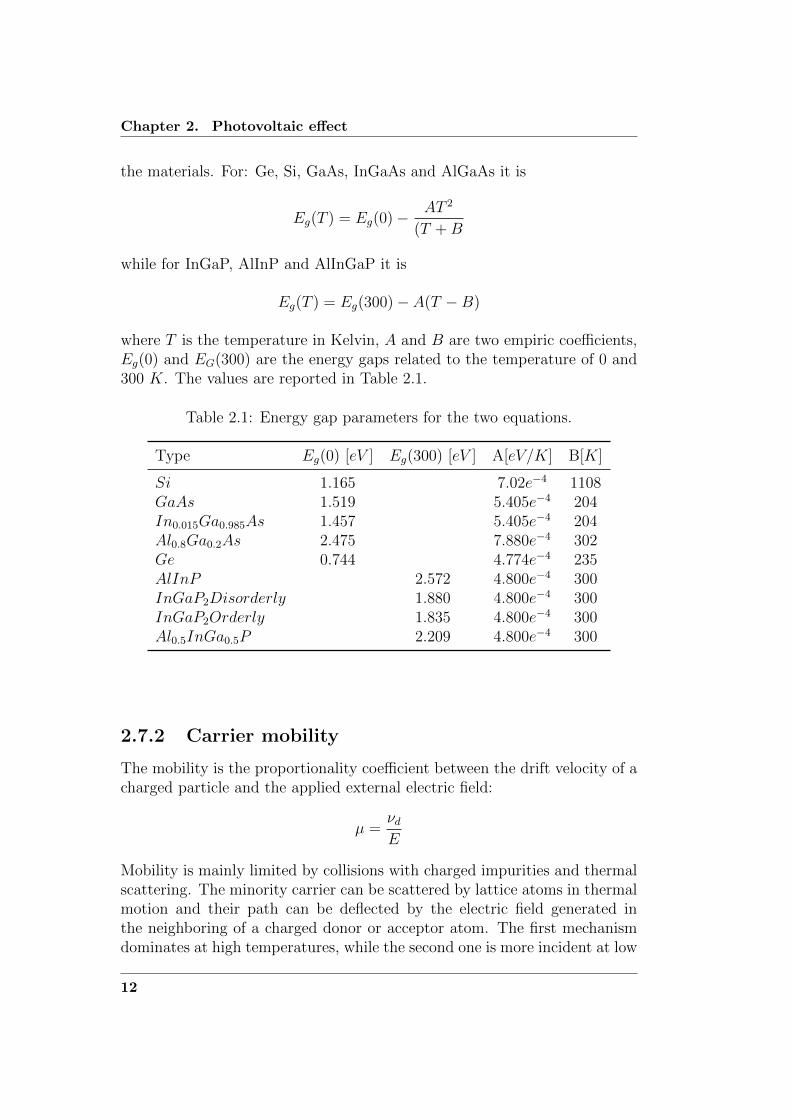
the materials. For: Ge, Si, GaAs, InGaAs and AlGaAs it is
Eg(T ) = Eg(0)− AT 2
(T +B
while for InGaP, AlInP and AlInGaP it is
Eg(T ) = Eg(300)− A(T −B)
where T is the temperature in Kelvin, A and B are two empiric coefficients,Eg(0) and EG(300) are the energy gaps related to the temperature of 0 and300 K. The values are reported in Table 2.1.
Table 2.1: Energy gap parameters for the two equations.
Type Eg(0) [eV ] Eg(300) [eV ] A[eV/K] B[K]
Si 1.165 7.02e−4 1108GaAs 1.519 5.405e−4 204In0.015Ga0.985As 1.457 5.405e−4 204Al0.8Ga0.2As 2.475 7.880e−4 302Ge 0.744 4.774e−4 235AlInP 2.572 4.800e−4 300InGaP2Disorderly 1.880 4.800e−4 300InGaP2Orderly 1.835 4.800e−4 300Al0.5InGa0.5P 2.209 4.800e−4 300
2.7.2 Carrier mobility
The mobility is the proportionality coefficient between the drift velocity of acharged particle and the applied external electric field:
µ =νdE
Mobility is mainly limited by collisions with charged impurities and thermalscattering. The minority carrier can be scattered by lattice atoms in thermalmotion and their path can be deflected by the electric field generated inthe neighboring of a charged donor or acceptor atom. The first mechanismdominates at high temperatures, while the second one is more incident at low
12

2.8. Solar intensity effect
temperature and in high doped material. The overall effect on the mobilitycan be approximated with the Matthienssen relation:
µ =
(1
µph+
1
µi
)−1Where the first term represent the thermal scattering and the second theimpurity scattering.Both for the GaAs cells and for the Silicon ones, mobility decreases withincreasing doping of the semiconductor, and the temperature dependencebecomes less sensitive.
2.7.3 Dark currents and lifetimes
Under operating conditions of solar cells, opposite to the photo generatedcurrent is generated a dark current, due to the establishment of a directbias voltage between its terminals. At the base of the dark current, whichgoes to deteriorate the performance of the solar cell, there are mainly threemechanisms of transport of carriers through the depletion region: diffusion,recombination and tunnel. The first two are depending on the temperatureand the third not (see [15] for more details).The lifetimes of minority carrier remain approximately constant over thetemperature of −50°C, for lower temperatures they drop slightly (for moredetails see [2]).
2.8 Solar intensity effect
If the temperature is held constant, the current output decreases linearlywith decreasing intensity, while the voltage output decreases logarithmically.The photo generated current (Jph), in fact, is directly proportional to thenumber of incident photons (F (λ)). As shown in the equation 2.1, this isexpressed by the integral over the incident wavelength range of the productbetween the density of incident photons and the cell quantum efficiency,being this last term the ratio between the number of generate carriers andthe number of incident photon per unit wavelength.
Jph = q
∫ ∞0
F (λ)QE(λ)dλ (2.1)
While the open circuit voltage depends on the short circuit logarithm.At lower solar insolation the leakage current becomes comparable with thephoto generated current and the shunt resistance assumes considerable im-portance, reducing the Fill Factor and the output voltage.
13

Chapter 2. Photovoltaic effect
2.9 Possible causes of performance loss in LILT
conditions
Solar cells which exhibit good performance in AM0 condition may have asignificant loss in fill factor, and thus in the power generator, in LILT condi-tions.This loss in fill factor is mainly due to two effects which show up under lowintensity and low temperature conditions: respectively the shunt effect andthe flat spot phenomena. The way these features affect the solar cell I-Vcharacteristic at LILT conditions is showed in Figure 2.9. The Flat Spot isrevealed as a triple slope in the IV curve (Broken-Knee), and its origin isassociated with a particular type of defect called Metal Semiconductor Like.
The shunt is a preferential path parallel to the junction for the current
Figure 2.9: Typical LILT degradation phenomena can become apparent un-der LILT measurement conditions.[19]
crossing the cell. Those paths can be caused by:
• Crystal defects on the surface of the cell which enable metal intrusionin the semiconductor from the metallization.
• Edge effects: typically defects created on the cell edge during the cellcut.
• Crystal defects that activate below a certain current density flow.
14

2.10. Radiation damage
• Doping diffusion from the tunnel layers.
• An excess of doping in the emitter or base layers.
2.10 Radiation damage
In an environment such as space, solar cells interact with particles withmass, high energy and possibly charge, such as electrons, protons, neutronsand ions.When one of these particles is absorbed by a material in general may occurseveral phenomena of interaction between the particle energy and the atomicstructure of the material [20].The dominant interactions are:
• Inelastic Collisions with Atomic Electrons. Inelastic collisions withbound atomic electrons are usually the predominant mechanism bywhich an energetic charged particle loses kinetic energy in an absorber.In such collisions, electrons experience a transition to an excited state(excitation) or to an unbound state (ionization).
• Elastic Collisions with Atomic Nuclei. Energetic charged particles mayhave coulombic interactions with the positive charge of the atomic nu-cleus through Rutherford scattering. In some cases the amount of en-ergy transferred to the atom will displace it from its position in a crys-talline lattice. If sufficient energy is transferred to displace an atomfrom its lattice site, that atom will probably be energetic enough todisplace many other atoms.
• Inelastic Collisions with Atomic Nuclei. Highly energetic protons un-dergo inelastic collisions with the atomic nucleus. In this process theenergetic proton interacts with the nucleus and leaves the nucleus in anexcited or activated state. The excited nucleus emits energetic nucleonsand the recoiling nucleus is displaced from its lattice site.
2.10.1 Ionization
The main types of radiation damage in solar cells are mainly due to ionizationand displacement of atoms.The ionization occurs when an electron in the outermost orbital is removedfrom the atom. To quantify the ionization radiation refers to the dose ofradiation absorbed by the material, expressed in rad (1 erg/g or 0.01 J/Kg).In this way different radiation exposure can be traced to the absorbed doses,
15

Chapter 2. Photovoltaic effect
reflecting the damage suffered by ionization in the material of interest. Forthe electrons absorbed, the dose is calculated from the incident fluence φ[e/cm2] (particles through the unit area integrated for a certain time).
Dose(rad) = 1.610−8dE
dxφ
where dEdx
[Mev·cm2
g] is the electron stopping power in the material of interest.
This concept can be applied to electron, gamma and X-ray radiations of allenergies, while for the protons only for those producing a homogeneous dam-age in the material, given that protons generally cause a damage localized inthe vicinity of the track of the particle.The main effect of ionization is the reduction of the coefficient of light trans-mission of cell’s coverage; the blackening is due to formation of color center-ing in the protection, and caused by excitation of electrons in the conductionband which end up trapped impurities in the atomic lattice. Other effectscaused by the ionization radiation may be leakage currents in the cell.
2.10.2 Atomic displacements
The atomic displacement is caused by the collision of fast particles in thecrystal lattice, so atoms are moved by their position in the lattice, whichgives rise to defects and imperfections that produce significant changes inthe equilibrium carrier concentrations and a minority carrier lifetime.The dislocation of the atoms requires a certain minimum amount of energy.When an incident particle has an energy equal to or greater than this thresh-old, the dislocation can be estimated with the following relationship:
Nd = naσνφ
where Nd is the number of displacements per unit volume, na the numberof atom per unit volume of absorber (5 · 1022 silicon atoms/cm3), σ thedisplacement cross section (cm2), ν the average displacements per primarydisplacement and φ the radiation fluence (particles/cm2).
2.10.3 Electron displacement damage
In the case of dislocation due to the electron it is possible to found in thelattice gaps whose distribution is not uniform. In fact the gaps left by sec-ondary dislocations lie relatively close to the primary gaps generated fromthe initial impact with the high energy particle.In n-type silicon, it has been shown that vacancies react with oxygen impu-rities to form close coupled vacancy-oxygen pairs, and with impurity donor
16

2.10. Radiation damage
atoms, such as phosphorus and arsenic, to form close coupled vacancy-donorpairs. Both defects are electrically active and can become negatively chargedby accepting an electron from the conduction band.
2.10.4 Proton displacement damage
The displacement generated by the protons is considerably different becausethe displacement cross sections are several orders of magnitude larger thanthose for fast electrons and vary rapidly with proton energy.The dislocation caused by the proton is highly inhomogeneous, since themany secondary dislocations occur near the site of the primary dislocation.
2.10.5 Neutron displacement damage
In the case of the neutron Coulomb forces are not involved but a collision ofthe rigid type occurs. The value of cross-section of displacement is smallerthan those of the electron and the proton, and this means that the numberof primary dislocations is smaller. In addition, the energy is transferred insupport of the reformation of the bonds between the atoms of the crystalstructure. The main importance of the displacement defects produced by
Table 2.2: Typical values of cross section dislocation in the silicon
Cross section dislocation
Electron 1 MeV 68 · 10−24cm2
Proton 1 MeV 3.5 · 10−20cm2
Neutron 1MeV 2.4 · 10−24cm2
the irradiation of silicon solar cells is in their effect on the minority carrierlifetime of the silicon. In particular, the lifetime in the bulk p-type silicon ofan n/p solar cell is the major radiation sensitive parameter.
17

Chapter 3
Rosetta mission
The Rosetta mission is designed to obtain the most detailed study of a cometever attempted. To reach this pourpose the Rosetta space probe is associ-ated to a lander, named Philae, which will attempt to make the frst-evercontrolled landing on a comet.The Rosetta mission was approved in 1993 by European Space Agency (ESA)Science Programme Committee, and it is one of the most important missionof the Horizon 2000 program.In the original mission plan Rosetta was set to be launched in January 2003to rendezvous with the comet 46P/Wirtanen, and to enter in orbit aroundit, in 2011. However, in December 2002 the planned launch vehicle Ariane5 turned out to be a failure. Therefore a new plan was made to target an-other comet, the 67P Churyumov–Gerasimenko (67P/CG), with launch on2 March 2004 and rendezvous in 2014.The mission name is taken from the Egyptian town of Rashid, or Rosetta,where, in 1979, archaeologists found a stone carrying inscriptions in three dif-ferent ancient languages. Archaeologists were able to decipher them thanksto the help of similar scripts on an obelisk from the town of Philae; thespacecraft’s lander has thus been named “Philae”. Indeed, space-scientistsof Rosetta mission wish to be as well successful as archeologists of Rosettastone in deciphering the data gathered from the 67P/CG comet [37].Rosetta mission is principally aimed at studying
1. the origin of comets,
2. the relationship between cometary and interstellar material,
3. its implications with regard to the origin and the evolution of the solarsystem.
To achieve these goals, the followings milestones (scientific objectives) havebeen defined: [6]:

3.1. Mission analysis
• Global characterization of the nucleus, determination of dynamic prop-erties, surface morphology and composition.
• Determination of the chemical, mineralogical and isotopic compositionsof volatiles and refractories in a cometary nucleus.
• Determination of the physical properties and interrelation of volatilesand refractories in a cometary nucleus.
• Study of the development of cometary activity and the processes in thesurface layer of the nucleus and the inner coma (dust/gas interaction).
• Global characterization of asteroids, including determination of dy-namic properties, surface morphology and composition.
3.1 Mission analysis
On 2 March 2004, after the reorganization of the mission due to the problemswith the Ariane 5 ECA launcher, Rosetta mission was successfully launchedby the Ariane 5 G+ from Kourou in French Guiana. The orbit which hasbeen inserted will bring in about ten years (4,300 days mission) to the comet67P/CG through a series of fly-by around some system Solar bodies. Thetimeline of the proposed assignment is described in table 3.1 whereas theRosetta orbit and the most important points of the mission are reported inFigure 3.1. It is important to note that during the period that Rosetta isorbiting the comet 67P/CG, the latter is going to reach the closest point tothe Sun in its orbit.During the mission period, the variation of the solar intensity is being calcu-lated on the basis of the following equation:
S ′ =S
d2
where “S” is the solar intensity of reference, “d” is the distance of Rosettaspacecraft from the Sun (it is measured in AU), and “S’ ” the relative solarintensity value.The expected values of distance between the Sun and Rosetta at differenttime-points of the entire mission period and the relative solar intensity valuesare reported in Figure 3.2 and in Figure 3.3.
Moreover, Figure 3.4 shows the trend of the solar intensity in SC for theperiod of operation of the Philae lander. At the beginning of Philae mission,the comet will be located between Mars and Jupiter orbits, so that the de-tected solar intensity values will be the lowest; instead, in a more advanced
19

Chapter 3. Rosetta mission
Figure 3.1: Graphical representation of the orbit of Rosetta [3].
20

3.1. Mission analysis
Table 3.1: The mission falls into several distinct phases [3].
Event Nominal date
Launch 2 March 2004First Earth gravity assist 4 March 2005Mars gravity assist 25 February 2007Second Earth gravity assist 13 November 2007Asteroid 2867 Steins flyby 5 September 2008Third Earth gravity assist 13 November 2009Asteroid 21 Lutetia flyby 10 July 2010Rendezvous manoeuvre 1 23 January 2011Enter deep space hibernation July 2011Exit deep space hibernation January 2014Rendezvous manoeuvre 2 between 4.5 and 4.0 AU 22 May 2014Start of near-nucleus operations at 3.25 AU 22 August 2014Lander Philae Delivery 10 November 2014Start of comet escort 16 November 2014Perihelion Passage August 2015End of nominal Mission 31 December 2015
Figure 3.2: Trend of the distance between Rosetta and the Sun, and the lightintensity [1].
21

Chapter 3. Rosetta mission
Figure 3.3: Trend of the solar intensity in W/m2 on Rosetta spacecraft duringall the mission time [1].
phase of the Philae mission, the comet will be positioned between Mars andthe Earth orbits, corresponding to its perihelion period, thus reaching itsmaximum values of solar intensity.
The minimum and the maximum solar intensity values that the lander
Figure 3.4: Trend of the solar intensity in SC for the period of operation ofPhilae on the comet [1].
would detect during the mission period are illustrated in Figure 3.2. It isimportant to consider that during the perihelion phase of its orbit, whichis expected in 2015, the comet 67P/ CG would be closest to the Sun thanduring its previous perihelion phase in 2002: i.e 1.2433 AU instead of 1.29
22

3.2. The comet
AU.
Table 3.2: Minimum and maximum solar intensity during the Philae periodon the comet.
Date SC Intensity [W/m2] Sun distance [AU]
Min 11/11/2014 0.11102 151.87 3.0013Max 13/08/2015 0.64695 885.03 1.2433
3.2 The comet
3.2.1 What is a comet
Comets are small, fragile, irregularly shaped bodies composed mostly of amixture of water ice, dust, and carbon- and silicon-based compounds. Theyhave highly elliptical orbits that repeatedly bring them very close to the Sunand then swing them into space. Comets have three distinct parts: a nucleus,a coma, and a tail. The solid core is called the nucleus, which develops acoma with one or more tails when a comet sweeps close to the Sun. Thecoma is the dusty, fuzzy cloud around the nucleus of a comet, and the tailextends from the comet and points away from the Sun. The coma and tailsof a comet are transient features, present only when the comet is near theSun [8].
3.2.2 Characteristics of 67P/CG
The comet 67P/CG was discovered in 1969, when several astronomers fromKiev visited the Alma-Ata Astrophysical Institute to conduct a survey ofcomets. On 20 September, Klim Churyumov was examining photographsof comet 32P/Comas Sola taken by Svetlana Gerasimenko when he found acomet-like object near the edge of the plate. He assumed that the faint ob-ject was the expected periodic comet, but upon returning to Kiev, he studiedthe plates very carefully and eventually realized that a new comet had beenfound, less than two degrees from comet Comas Sola.
The comet has a particularly unusual history. Up to 1840 its periheliondistance was 4.0 AU (four Sun-Earth distances or about 600 million km)and the comet was completely unobservable from Earth. That year, a fairly
23

Chapter 3. Rosetta mission
Figure 3.5: Discovery image of comet 67P/Churyumov–Gerasimenko in 1969[9].
close encounter with Jupiter caused the orbit to move inwards to a periheliondistance of 3.0 AU (450 million km). Over the next century, the periheliongradually decreased further to 2.77 AU. Then, in 1959, a further Jupiter en-counter reduced the perihelion to just 1.29 AU. It currently completes oneorbit of the Sun every 6.57 years.The comet has now been observed from Earth on six approaches to the Sun- 1969 (discovery), 1976, 1982, 1989, 1996 and 2002. It is unusually activefor a short period object and it has a coma (a diffuse cloud of dust and gassurrounding the solid nucleus) and often a tail at perihelion. During the2002/2003 apparition, the tail was up to 10 arcminutes long as seen fromEarth, with a bright central condensation in a faint extended coma. Even7 months after perihelion the tail continued to be very well developed, al-though it subsequently faded rapidly.The comet typically reaches a magnitude around 12, although this is be-cause the comet has outburst at perihelion at three of its last four returnsin 1982/83, 1996/97 and 2002/03. Despite being a relatively active object,even at the peak of outburst the dust production rate is some 40 times lowerthan for 1P/Halley. Nevertheless, 67P/CG is classed as a dusty comet.
24

3.2. The comet
The peak dust production rate in 2002/03 was estimated at approximately60kg per second, although values as high as 220kg per second were reportedin 1982/83. The gas to dust emission ratio is approximately 2.[6]Sixty-one images of comet 67P/CG were taken with the Wide Field Plane-tary Camera 2 on board the Hubble Space Telescope (HST) on 11-12 March2003. The HST’s sharp vision enabled astronomers to isolate the comet’snucleus from the coma. The images showed that the nucleus measures fiveby three kilometres and has an ellipsoidal (rugby ball) shape. It rotates oncein approximately 12 hours. It is composed of a highly porous mixture, incertain percentages of ice of water (the main component), CO2, CO, carboncompounds, nitrate and silicate dust. The main characteristic of the 67P/CGcomet are reported in the Ttable 3.3.
Table 3.3: Comet 67P/CG parameters [6].
Comet 67P/Churyumov-Gerasimenko
Diameter of nucleus - estimated (km) 3 x 5Rotation period (hours) ∼ 12Orbital period (years) 6.57Perihelion distance from Sun (million km) 194 (1.29AU)Aphelion distance from Sun (million km) 858 (5.74AU)Orbital eccentricity 0.632Orbital inclination (degrees) 7.12Year of discovery 1969Discoverers Klim Churyumov and
Svetlana Gerasimenko
3.2.3 The nucleus
The evolution of the nucleus is governed, first, by heat transfer due to con-ductive and radiative transfer, and second, by exchange of latent heat dueto the motion of the gas through the porosity, and heat received through thesurface in dependence on its thermo-optical properties (such as albedo andemissivity), in particular by the percentage coverage of the crust of dust, andby the distance of the Sun.At the beginning of its life, the comet’s nucleus can be described as a simpleand homogenous body. Instead, during the approach to the Sun, the energy
25

Chapter 3. Rosetta mission
input through the surface increases the temperature and the ice begins tosublimate, the first component that begin to sublimate is CO, followed byCO2, while H2O requires higher temperatures. The sublimation of the iceallows the expulsion of dust particles from the nucleus, or their return on thesurface, this depending on the forces into play. All these mechanisms lead tothe formation of crust of dust and to the differentiation of substrates. Underthe crust, which may or may not be present in different percentages, stillpersist a homogeneous nucleus [1].
3.2.4 Study of the comet
Following the designation of the 67P/CG comet as the new target of Rosettamission, space-scientists started to study the physical, geometrical and chem-ical characteristics of that comet. The most important observations theymade are listed below:
• European Southern Observatory and Very Large Telescope (VLT) at LaSilla in Chile, between 11 February 2003 and 26 June 2003: spectrummeasurements - photometry to determine the rate of production of gasand dust.
• Hubble Space Telescope (HST), January 2003: observations to deter-mine the nucleus (assumed value of albedo), the rotation period andthe color index.
• Spitzer Space Telescope : observations to determine the thermal emis-sion of the comet 67P/CG. These measurements combined with thosein the visible allowed the use of the radiometric techniques to derive thesize and the albedo (correlated which is correlated with the estimate ofthe first.
• European Southern Observatory with the New Technology Telescope(NTT), 3.5 m (2005): Photometry in the visible to measure the periodof rotation, the effective radius, the phase function and the color.
3.2.5 Radiation on the comet
Radiation may be defined as the emission and propagation of energy throughfree space or through a material medium. The space radiation environment iscomposed of cosmic rays, electromagnetic radiation, Van Allen belt radiation,auroral particles, and solar flare particles.The study of radiation is critical for determining the electrical behavior of
26

3.2. The comet
the Solar cells; in fact, the radiation causes strong degradation which isdependent on the type of radiation encountered and on the residence time ina given area of space.Radiation in interplanetary space consists of an energetic cosmic flux andpulses of radiation associated with solar flares. In addition to these sources ofinterplanetary radiation, there also exist a continuous ejection of low energyparticles from the sun (primarily protons and electrons) known as the solarwind. The distribution of the solar wind particles is assumed to obey theinverse-square law with the sun acting as a point source.Cosmic rays of galactic origin consist of protons (∼ 93%) and alpha particles(∼ 7%) along with smaller amounts of heavier elements. Proton (p+) is apositively charged particle of mass number 1 (having a mass of 1.672 x 10⁻²⁷
kg) and a charge equal in magnitude to the electron (i.e. 1.602 x 10⁻¹⁹
coulombs); it is also the nucleus of a hydrogen atom. Alpha particle (alpha)is a positively charged particle identical to all properties of the nucleus of ahelium atom, consisting of two protons and two neutrons. The energy of theprotons is in the range of 5 x 10⁸ eV to 2 x 10¹⁰ eV. Although energies arequite high, the free space flux of particles is 2.5 particles pro cm−2s−1. Sincethis flux is small, radiation damage due to cosmic rays usually needs to beconsidered only on very long space flights [5].
3.2.6 Dimensions and shape
In order to determine the size and shape of the nucleus of the comet 67P/CG,astronomers have performed multiple visual observations of the comet withthe Hubble Space Telescope (HST) and the New Technology Telescope (NTT),and also infrared observations with the Spitzer Space Telescope (SST). Thesize and shape have been then obtained by inverse analyses of photometriclight curves in function of time.The measurements made in the visible through HST and NTT first let tothe prediction of two independent models of nuclear shape and size underthe following assumptions:
1. value of geometric albedo1 of 0.04
2. coefficient phase2 of 0.04 mag/deg.
1The geometric albedo of an object is defined as the ratio of the brightness at α = 0 (αphase angle, i.e. the angle between the light source and the observer), and the brightnessof an ideal flat surface, completely reflective and diffusive, with the same cross section.
2Relative to the phase function j(α) which gives the ratio of the intensity diffuse in thedirection of alpha respect to the intensity diffused to α = 0
27

Chapter 3. Rosetta mission
Those models, indeed resulting from a limited amount of information, arethe best-fitting from the observations made up to 2006 and predict an highlyirregular area for the comet 67P/CG.Under given constraints of smoothness of surface and inertia matrix (suchas rotation about the main axis), the two models of nuclear shape can berepresented graphically in three dimensions, one prograde and one retrograde,as shown in Figure 3.6.According to these models, the rotation period of the comet 67P/CG would
Figure 3.6: The prograde (top row) and the retrograde (bottom row) solu-tions for the threedimensional shape of the nucleus of comet 67P/CG recon-structed from the inversion of the 2003 HST and 2005 NTT light curves. Foreach solution, three views of the reconstructed 3-D shape model are displayedat three different rotational phase angles: 350°, 80°, and pole-on view of the80° model [33].
be 12.68 ± 0.03 hours and the orientation of the rotational axis would bedefined. Indeed, thanks to the observations of the heat flow through theSST, it has been possible to remove the uncertainty of the albedo value, andthereby to obtain a better estimate of the nuclear size of the comet.The Table 3.4 shows the best estimates of physical parameters, obtained fromthe observations made until 2006. In particular, the density of the nucleuswould be in a range between 100 and 500 kg/m3, with a most likely value of370Kg/m3. It also provides the moments of inertia and the coefficients of thesecond degree and order C20 and C22 harmonic expansion of the gravitationalfield of the model calculated.
28

3.2. The comet
Figure 3.7: Light curves from HST and NNT. The dots represent the recordeddata and lines the best-fit for the two solutions [9].
Table 3.4: Principal physical parameters for the comet 67P/CG.
Solution Prograde Retrograde
x length 4.74km 4.49kmy length 3.77km 3.53kmz length 2.92km 2.93kmVolume 21.2km3 21.3km3
Area 40.2km2 40.1km2
Mass (500kg/m3) 1.0e13kg 1.0e13kgMass (100kg/m3) 2.1e12kg 2.1e12kgMass (5370kg/m3) 7.8e12kg 7.9e12kgInertia ratio Ix/Iz 0.7 0.67Inertia ratio Iy/Iz 0.86 0.86C20 −0.33/r20 −0.35/r20C22 0.060/r20 0.060/r20
29

Chapter 3. Rosetta mission
3.2.7 Axis of rotation
The nuclear rotational axis of the comet 67/CG has been studied by variousastronomers using different techniques .Each technique used as a starting point some of the constraints that must bemet by the resulting light curves and different view geometries observed fromthe nucleus structure (jets, fans, shells, etc.). To determine the direction ofthe rotational axis is necessary to provide two angles that can be expressedwith respect to the ecliptic coordinates (λ and β), or in terms of right ascen-sion and declination (AR and δ). Maybe the most known hypothesis havebeen found by Lamy [9] ; through the HST light curves he identified 4 hy-pothesis, two of which are indeed improbable: the first (likely) hypothesis fitswith the prograde solution and identifies λ = 51°±20° and β = 54°±10° andcorresponds to a clockwise rotation; the second likely hypothesis fits withthe retrograde solution and identifies λ = 245°±20° and β = −50°±10° andcorresponds to an anticlockwise rotation.Additional likely hypotheses for the nuclear rotational axis of the comet67/CG have been proposed by Davidsson and Gutierrez [10]; by using athermo-physical model and by applying all the constraints inferred by theobservations, they have identified two likely intervals for the rotational axis:the first interval is defined by an obliquity (the angle between the spin axisand the angular momentum vector of the cometary orbit) of 120 ° ±30 ° anda topic (the clockwise angle from the point of the vernal equinox of the cometand the subsolar meridian at perihelion) of 60° ±15° ; the second interval ischaracterized by a skew of 60°±30° and an argument of 240°±15°. Other in-teresting solutions have been proposed by Chesley (2004), Schleicher (2006)and Weiler (2004) [9].Taken together the proposed hypotheses led to the idea that the orientationof the rotational axis is included in a region expressed in celestial coordinatesRA = 220°(+50° /− 30°) and δ = −70° ±10° (counterclockwise rotation) orin a region expressed in celestial coordinates AR = 40° (+50°/ − 30°) andδ = 70°±10° (clockwise rotation). Figure 3.8 summarizes the so far proposedlikely solutions.
3.2.8 Shadow in a crater
The time-window of light availability on the surface of a comet is an impor-tant parameter to take in account when landing on a comet. Since cometshave craters on their surface, the time-window of light availability is pre-dicted by determining the length of the shadow cast by crater walls [11]; theshadow length is measured on the floor of the depression from the central
30

3.2. The comet
Figure 3.8: Constraints on the direction of the rotational axis of the nucleusof comet 67P/Churyumov-Gerasimenko as determined by different authors[9].
rim to the crater wall along the direction θ, and is currently calculated byusing a simple geometric condition resulting in the following relationship:
rsh = −zd tanα cos(θ − ζ
)±(r2d − z2d tan2 α sin2
(θ − ζ
))0.5
where dr is the distance from the crater wall to the crater center measuredon the floor of the depression, dz is the crater depth and the angle ζ is theazimuth of the Sun. Here the plus sign indicates the case in which the cratercenter is illuminated.
3.2.9 Gas production
The measurements made during the 1982 and 1996 apparitions, which oc-curred when 67/CG was at its perihelion, let to determine the productionrate of five gas species: OH (used for calculating the production rate ofH2O), CN , C2, C3, and NH. Instead, during the 2002 apparition only asingle measurement for the CN has been collected.As illustrated in Table 3.5, the authors which have contributed to the spectrameasurements to assess the gas production rates of 67/CG are many [9].
The production rate of some species can be approximated by the method
31

Chapter 3. Rosetta mission
Table 3.5: Measurements of production rates by various authors.
Authors and year Species
Cochran (1992) CN,C2, C3
Storrs (1992) CNOsip (1992) OH,CNSchleicher (2006) OH,CN,C2, C3, NHHanner (1985), Crovisier (2002), Makinen (2004) OHWeiler (2004), Schulz (2004) CN
Figure 3.9: Observed gas production rates versus time from perihelion forComet 67P/Churyumov–Gerasimenko [9].
of least squares, which leads to the following equation:
log10(Qx) =3∑i=0
ai
(T − b1b2
)iWhere Qx is the speed of production of the gas species X expressed inmolecules/sec, T is the number of days from perihelion (which is a positivevalue if it refers to the post-perihelion period), and a and b are species-specificcoefficients.If“T” falls outside the range of validity, a simplified formula can be used (but
32

3.2. The comet
only as a first approximation):
Qx = Ajr−Bj
h
Where A and B are species-specific and also perihelion period-specific coef-ficients, meaning that their value depend also on the considered perihelionperiod ( pre- or post-perihelion).
3.2.10 Dust production
Dust is one of the main elements presents in the emissions from the cometarysurface. Attaining an adequate level of exposure to dusts is of decisive im-portance for the achievement of some goals of Rosetta mission; however, theimpact or the deposit of dust on some sensitive surfaces of the satellite maybe dangerous for its activity and may thereby cause a failure of the mission.When previous investigative missions, such as Giotto and Deep Impact, madetheir close approach to the comets, the space probes were hit by large sizedust particles, mainly in the order of a few millimeters, which damaged someof their scientific sensors and caused a relevant deviation from their desiredattitude. However the approach speed of Giotto and Deep Impact was muchhigher (in the order of Km/s) than that expected for Rosetta (a few m/s).It is therefore necessary to have a model of the foliage of 67P/CG order topredict the flow and the speed of the powders inside a function of time andspace. Through a study of the flow of the powders is also possible to havean estimation of the level of light radiation on the surface, so going to checkthe operating conditions of the solar panels of the lander Philae.Several authors have addressed this problem [12] [13] by recovering theparameters required by astronomical observations or using those of othercomets, such as those measured in-situ for comet Halley explored by Giottoin 1986 (such as the mass distribution). From the data of similar comets itcan be seen that water and CO are the main elements of the gases, while thepowder particles are formed by silicates and carbonaceous materials with asize ranging from a few nanometers to millimeters.To go back to the production of powder of a comet were used the parameterAfρ that is obtained by photometric observations and defined as the productof the albedo (the reflectivity of the grain), fill factor (related to the opticaldensity of the foliage, it describes how much occupies the canopy than thefield of view) and ρ (radius of the crown). The parameter Afρ is related tospeed of production Qd,j relative of to the particle size Sj with the emissionrate vd,j, to the value of albedo geometric p and the phase function j(α),
33

Chapter 3. Rosetta mission
according to the relation:
Afρ = 2πpj(α)∑j
s2jQd,j
vd,j
The albedo geometric p and the phase function j(α) link the cross-sectionof a particle of dust with the light diffused by it. The phase angle α is theangle between the direction of the observer and that of the incident radiation,viewed from the particle that spreads. The geometric albedo of an object isdefined as the ratio of the intensity reflected back from the object, α = 0,and the total intensity diffused. The phase function j(α) provides the ratioof the intensity diffused in the direction α respect to the intensity diffusedto α = 0. For the 67P/CG is considered the function of geometric phaserepresented in Figure 3.10 , assuming a geometry emission axial-symmetricwith peak activity in the subsolar point. This hypothesis is required and
Figure 3.10: Solid line: phase function of an individual dust particle asgiven in Divine (1981), but here normalised to j(α = 0) = 1. Dashed line:geometric phase function jgeo(α) Muller (1999) [13].
the reason is that if an observer looks in the direction perpendicular to thedirection of emission of the particle, this will tend to leave the field of viewvery quickly than when you look in a parallel direction. Hence the number ofparticles inside the field of view (which may dramatically influence the valueof Afρ measured) depends on the angle between the direction of emission ofthe particles and the direction of the observer.The values of Afρ measured for 67P/CG were recorded during its approachto perihelion of 1982/1983, 1996/1997 and 2002/2003 by several authors(Storrs 1992; Osip 1992; A ’Hearn 1995; Kidger 2003; Lamy 2003; Weiler2004; Schulz 2004; Feldman 2004; Schleicher 2006) and the results are shownin Figure 3.11 as a function of days at perihelion. By adopting the correctionphase angle for the geometric phase function were obtained values for Afρ
34
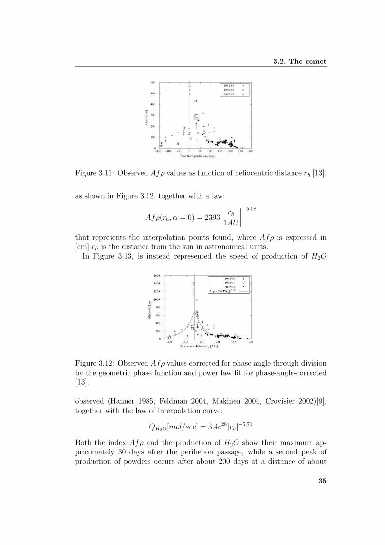
3.2. The comet
Figure 3.11: Observed Afρ values as function of heliocentric distance rh [13].
as shown in Figure 3.12, together with a law:
Afρ(rh, α = 0) = 2393
∣∣∣∣ rh1AU
∣∣∣∣−5.08that represents the interpolation points found, where Afρ is expressed in[cm] rh is the distance from the sun in astronomical units.
In Figure 3.13, is instead represented the speed of production of H2O
Figure 3.12: Observed Afρ values corrected for phase angle through divisionby the geometric phase function and power law fit for phase-angle-corrected[13].
observed (Hanner 1985, Feldman 2004, Makinen 2004, Crovisier 2002)[9],together with the law of interpolation curve:
QH2O[mol/sec] = 3.4e28|rh|−5.71
Both the index Afρ and the production of H2O show their maximum ap-proximately 30 days after the perihelion passage, while a second peak ofproduction of powders occurs after about 200 days at a distance of about
35

Chapter 3. Rosetta mission
2.5 AU. Soon after, between 2.5 and 3 AU may be noted a sharp decline inproduction of dust, and beyond 3 AU all the checks show a pointed nucleus[14].
Figure 3.13: Measured H2O production rates with corresponding power law[13].
3.2.11 Dynamics of comet dust
A comet is an agglomeration of ice and dust. When the comet reaches thedistance of about 3 AU, the ice near the surface begins to sublimate releasingthe dust trapped in it. Inside the canopy, within a few rays from the surfaceof the nucleus, the motion of the powder grains is coupled with the flowof gases emitted from the nucleus and are accelerated; over ten times theradius of the core expanding gas becomes too diluted to exert an appropriateforce and the flow of powder is decoupled from that of the gas; in this zonethe particles have reached their maximum speed, said final speed, which isproportional to 1√
ρswhere ρ is the density of the particle of radius s, and is
used to interface the part of the crown in which case the acceleration of theparticles, dominated by the forces of emission and the severity of the nucleusof the comet, with the part where the dynamics is governed by radiationpressure and the severity of the Sun.In addition to the canopy, the powders form the typical tail direct in theopposite direction to the Sun, because of the pressure of radiation, withinwhich the position of the particle is a function of the pressure coefficient ofβ radiation and the emission time. The coefficient β takes into account theradiation pressure and the gravity of the Sun, and it is defined as:
β =3L
16πcGM
Qpr
ρs
36

3.2. The comet
Where L and M are the luminosity and the mass of the Sun, c is the speedof light, G is the gravitational constant and qpr is the efficiency of the radia-tion pressure, that represents the properties of absorption and scattering ofgrain averaged over the entire solar spectrum and depends on the material.In order to understand the formation of dust tails, the concepts of synchronesand syndynes were introduced by Bredikhin (1903). Synchrones are the po-sitions of particles of different β emitted at a given time, while syndynesdescribe the positions of particles of fixed β and varying emission time. Bothterms refer to hypothetical particles emitted with zero velocity relative tothe nucleus. Since, realistically, the initial velocity of a dust grain is differentfrom zero, the resulting synchrone or syndyne will have a finite cross sectionwith a radius proportional to the product of dust emission speed and timeelapsed since emission. In particular, grains released at a given time withisotropic speed will form a spherical shell the centre of which moves alongthe appropriate syndyne.While for particle sizes on the order of the dominant wavelengths of the solar
Figure 3.14: Synchrones are shown projected in the comet orbit plane (left)and image plane (right). The solid lines correspond to synchrones for dif-ferent period of times, the dashed lines correspond to syndynes for differentvalues of β [13].
spectrum (0.01 ... 1µm) β depends sensitively on material, shape, structureand size of the particles (Burns et al., 1979), it is about constant for muchsmaller particles and proportional to 1
ρsfor large ones, i.e. in the geometric
optics regime (Gustafson, 1994) [13].In the literature, both the exponents γ of the cumulative mass distributionF (m) ∼ m− γ and α of the differential size distribution g(s) ∼ sα are com-monly used. If a constant particle bulk density is assumed in the concernedinterval, the exponents γ and α are related as α = −3γ − 1.In Table 3.6 are shown the exponents determined by several authors through
37

Chapter 3. Rosetta mission
the use of photometric observations of the comet 67P/CG and by in-situmeasurements of other comets (Halley 1986), while the Figure shows thechart who sets the trend of the percentage of particles as a function of size.Agarwal proposed different mathematical models which allow to reproduce
Table 3.6: Values of α and γ found in the literature.
α γ
Divine and Newburn −4.3 1.1Agarwal −3.7 0.9Fulle −3.3 0.8
Figure 3.15: Number fraction over particle radius for the three differentialsize distributions [13].
the evolution of the canopy and the mass flow emitted. The first simpli-fied model is defined as a model radialsymmetric in which the activity ofthe surface is uniformly distributed on the surface of the comet; the secondis a model based on insulation (Insulation driven), for which the surface ishomogeneous and issuing activity is proportional to the amount of radiationreceived; finally the model jets, in which the activity on the surface of thecomet is described by a Gaussian centred in the subsolar point.Additionally, for all models is considered a core of spherical shape of radius2 Km in which the grains of powder are divided into classes depending onthe mass, and is also considered to be a constant density for grains of 1000Kg/m3. In a first step is calculated by the flow of gas, at which the pow-der is coupled at least in the instants immediately after issuance from thenucleus; thereafter the trajectories of the grains are integrated consideringthe severity of the core and the resistance force exerted by the gas. For sim-plicity gases are considered H2O and CO, whose production speed are used
38

3.2. The comet
as input to the model, together with the values of Afρ, the phase function,mass distribution and final velocities determined.
3.2.12 Optical opacity due to dust
A study of optical opacity due to dust has been carried out in accordance withthe standard Insulation driven and jets [13]. The optical opacity (OpticalDepth, τ) is a measure of transparency and expresses the amount of lightremoved from a radius by diffusion or absorption. If I0 is the intensity oflight at the source, and I is the intensity of light observed after a certainpath, τ is defined by the following expression:
I
I0= e−τ
The optical opacity in the case of a comet is influenced by the parametersAfρ, phase function, albedo of dust and efficiency of extinction. The firstthree parameters are easily obtained through observations from Earth, whilefor the last estimate is a value between 1 and 2. For the optical opacityhas been identified, for the worst conditions, a maximum value of 0.2, takinginto account the line of sight to the Sun-surface of the nucleus in the subsolarpoint at perihelion, considering the model jet, then the most burdensome.Since the optical opacity is proportional to the value of Afρ, by the law ofinterpolation, has determined a value of τ for all the way from the cometat 3 AU until perihelion as shown in the Figure 3.16, while in the Figure3.17 is shown the trend light intensity as a function of distance from the Sunconsidering the optical opacity calculated.
Figure 3.16: Trend of the value of Afτ and τ as a function of distance fromthe Sun [1]
.
39

Chapter 3. Rosetta mission
Figure 3.17: Performance of the light intensity with and without τ as afunction of distance from the Sun [1].
3.2.13 Lighting conditions
At this point it is possible to make some reasonable assumptions and calculatethe variation of the light radiation on the surface of the comet 67P/CG afunction of time. Considering only the period of the mission of the landerPhilae (counting the day of landing), 10 November 2014, as the first day oras −276 day before the perihelion of the comet that will be at 13 August2015. Shall be adopted various hypotheses derived from the discussions inthe preceding paragraphs, including the inclination axis, which is directedtoward the north right ascension of 40° and declination of 70°. The periodis assumed, as mentioned earlier, of a duration of 12.68 hours. Also forsimplicity is assumed a spherical shape for the nucleus of the comet. Withthe choice made on the axis will be had the spring equinox (here correspondsto a aerocentric longitude at 0°) on 13 March 2015 (which correspond tothe 123 days of the mission of the lander) and the autumnal equinox on 26December 2015. The value of optical opacity τ assumes variable and followsthe trend described in the previous section, while in the first approximationthe contribution of the scattered light is considered negligible. A solar panelon the surface of the comet will then receive a light radiation equal to:
I(r, τ, δ, φ, dφ, w, dw) =
i(r)−τmz sin(φ+ dφ) sin(δ) + cos(φ+ dφ) cos(δ) cos(w + dw)
Where I(r) is the total light radiation at a distance r of the comet from theSun, mz is the air mass (in this case we consider the comet’s coma as anatmosphere), φ is the latitude and dφ is the tilt angle of the solar panel tothe north, δ is the declination of the Sun, then w is the hour angle of theSun (= 0 at noon) and dw is the inclination of the panel towards the east.
40

3.2. The comet
Whereas a horizontal panel relative to the surface of the comet. Considering
Figure 3.18: Light intensity of the soil of the comet as a function of the daysat perihelion. Are indicated respectively, the day of the lander landing, thespring equinox, the perihelion and the nominal end of mission, 31/12/2015[1].
the landing equator we can calculate the radiation intensity during the hoursof the day, for example for the first 10 days of mission is obtained the graphof Figure 3.19. In addition, by calculating the vector Sun, always starting
Figure 3.19: Light intensity on a horizontal panel during the first 10-daymission at the equator [1].
from the equator landing day until the day of perihelion, is obtained thegraph of Figure 3.20.
41
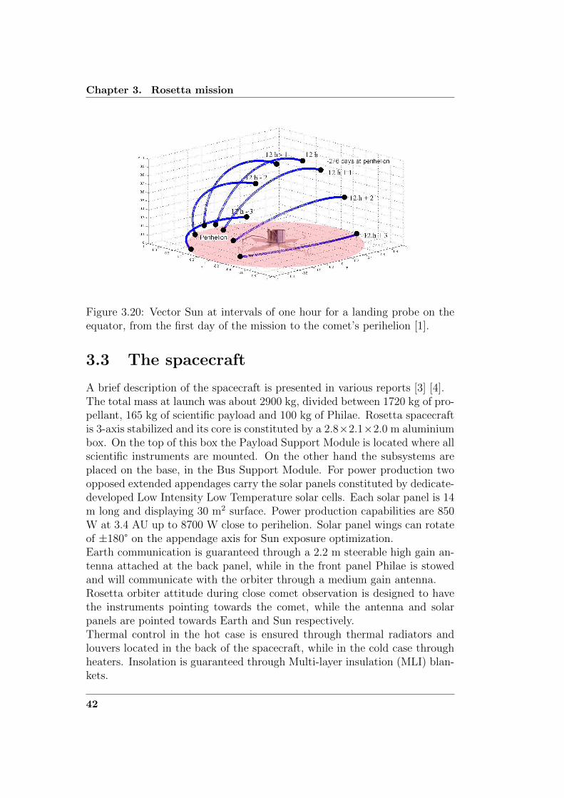
Chapter 3. Rosetta mission
Figure 3.20: Vector Sun at intervals of one hour for a landing probe on theequator, from the first day of the mission to the comet’s perihelion [1].
3.3 The spacecraft
A brief description of the spacecraft is presented in various reports [3] [4].The total mass at launch was about 2900 kg, divided between 1720 kg of pro-pellant, 165 kg of scientific payload and 100 kg of Philae. Rosetta spacecraftis 3-axis stabilized and its core is constituted by a 2.8×2.1×2.0 m aluminiumbox. On the top of this box the Payload Support Module is located where allscientific instruments are mounted. On the other hand the subsystems areplaced on the base, in the Bus Support Module. For power production twoopposed extended appendages carry the solar panels constituted by dedicate-developed Low Intensity Low Temperature solar cells. Each solar panel is 14m long and displaying 30 m2 surface. Power production capabilities are 850W at 3.4 AU up to 8700 W close to perihelion. Solar panel wings can rotateof ±180° on the appendage axis for Sun exposure optimization.Earth communication is guaranteed through a 2.2 m steerable high gain an-tenna attached at the back panel, while in the front panel Philae is stowedand will communicate with the orbiter through a medium gain antenna.Rosetta orbiter attitude during close comet observation is designed to havethe instruments pointing towards the comet, while the antenna and solarpanels are pointed towards Earth and Sun respectively.Thermal control in the hot case is ensured through thermal radiators andlouvers located in the back of the spacecraft, while in the cold case throughheaters. Insolation is guaranteed through Multi-layer insulation (MLI) blan-kets.
42

3.3. The spacecraft
For propulsion 10 bi-propellant thrusters of 24 N are used, and can be alsoexploited for attitude control. [16]The scientific instruments on board of the Rosetta orbiter are [3]:
• ALICE An ultraviolet imaging spectrograph (Alan Stern, SRI, Boul-der (USA))
• OSIRIS Optical, Spectroscopic, and Infrared Remote Imaging System(Horst-Uwe Keller, MPS, Lindau (D))
• VIRTIS Visible and Infrared Thermal Imaging Spectrometer (Angio-letta Coradini, IAS-CNR, Rome, (I))
• MIRO Microwave Instrument for the Rosetta Orbiter (Sam Gulkis,JPL, Pasadena, (USA))
• CONSERT Comet Nucleus Sounding Experiment by Radiowave Trans-mission (Wlodek Kofman, LPG, CNRS/UJF, Grenoble (F))
• ROSINA Rosetta Orbiter Spectrometer for Ion and Neutral Analysis(Hans Balsiger, Universitat Bern (CH)
• MIDAS Micro-Imaging Dust Analysis System (Willi Riedler, IWF,Graz, (A))
• COSIMA Cometary Secondary Ion Mass Analyzer (Martin Hilchen-bach (formerly Jochen Kissel), MPS, Lindau (D))
• GIADA Grain Impact Analyzer and Dust Accumulator (Luigi Colan-gelo, INAF, Naples (I))
• RPC Rosetta Plasma Consortium (Anders Eriksson (formerly RolfBostrom), IRF Uppsala IRF Uppsala, (S), Jim Burch, SRI, San Anto-nio, (USA), Karl-Heinz Glassmeier, IGEP, Braunschweig, (D), RickardLundin, IRF, Kiruna (S), Jean-Gabriele Trotignon, LPCE/CNRS, Or-leans (F), Chris Carr, Imperial College, London (ENG))
• RSI Radio Science Investigation (Martin Patzold, Universitat Koln(D))
43

Chapter 3. Rosetta mission
Figure 3.21: The Rosetta spacecraft and its scientific payload [3].
3.4 The lander Philae
The lander Philae will investigate the comet 67P/CG in-situ, while the spaceprobe Rosetta will operate from orbit. The Lander system has been providedby an international consortium (Germany (lead), France, Italy, Hungary,Finland, UK, Ireland and Austria) and supports a scientific payload of 10instruments [39]. It is operated by the Lander Control Center (LCC) atDLR, Cologne, and the Science Operation and Navigation Center (SONC)at CNES, Toulouse, via the European Spacecraft Operations Center (ESOC)in Darmstadt. Since the launch the lander has been operational during com-missioning, by performing several checkout as well as some activities forcalibration and failure investigation. The location of Philae in the Rosettaconfiguration is visible in 3.21.All the manoeuvres during flight are performed by Rosetta, while Philae isprepared to the descent and on-comet operations. The lander entered in thehibernation phase together with the space probe pending to reach the targetcomet. However separation, descent and landing strategy are not yet fullyoutlined as there’s the necessity to characterize first the comet nucleus fromorbit, where shape, state of rotation, gravitational field as well as gas anddust environment are relevant key parameters.The deployed configuration of the Lander is visible in Figure 3.22. The lan-der is designed to detach itself from the main spacecraft and fall towards thecomet along a ballistic trajectory (see Figure 3.23). To reduce the chanceof bouncing during initial impact the legs are designed to damp during thelanding, and to avoid possible detachment from the comet surface it will
44

3.4. The lander Philae
harpoon itself to it. Eventually is possible to activate a motor on the Lid toobtain a tighter anchoring to the comet nucleus. The lander main operative
Figure 3.22: Rosetta Lander, Philae, in landed configuration [32].
Figure 3.23: Philae landing scenario [30].
phases are Separation, Descent, and Landing (SDL), First Science Sequence(FSS) and Long Term Science (LTS). The first two phases last for 5 cometdays (i.e. about 60 hours) after the separation from Rosetta space probe and
45

Chapter 3. Rosetta mission
the power demand is satisfied by the primary battery. The LTS instead willlast depending on the success of the Solar Array System (SAS) to producepower [32]. The total mass is about 100 kg, and most of the surface is coveredwith solar cells, with the objective of extending LTS by providing additionalpower to the PSS (Power SubSystem) to charge the secondary battery.The scientific objectives of the Lander are the determination of the compo-sition of cometary surface matter, including the possible presence of organicmaterials, as well as the investigation of the structure and physical, chemicaland mineralogical properties of a comet’s surface, including the local depthstructure (stratigraphy) and global internal structure of a comet’s nucleus.Communication with Earth of all the data and the telemetry will be throughthe high gain antenna on Rosetta space probe, which will function as com-munication bridge. [17]The Rosetta lander scientific instruments are [3]
• APX Alpha Proton X-ray Spectrometer (G. Klingelhofer/R.Rieder;University of Mainz/ Max Planck Inst. (D))
• COSAC The COmetary SAmpling and Composition (F. Goesmann,H. Rosenbauer; MPS, Max Planck Inst. (D))
• Ptolemy Evolved Gas Analyzer (I.Wright, C.Pillinger, J.Zarnecki; OpenUniversity (UK))
• CIVA Comet Nucleus Infrared and Visible Analyzer (J.P.Bibring; IAS(F))
• ROLIS Rosetta Lander Imaging System (S.Mottola; DLR (D))
• CONSERT COmet Nucleus Sounding Experiment by Radiowave Trans-mission (W.Kofman; LPG (F))
• MUPUS MUlti-PUrpose Sensors for Surface and Sub-Surface Science(T.Spohn; University of Munster (D))
• ROMAP Rosetta Lander Magnetometer and Plasma Monitor (U.Auster,I.Apathy; Max Planck I. extraterr. Physics, TU Braunschweig(D)/KFKI (H))
• SESAME Surface Electric Sounding and Acoustic Monitoring Experi-ment (K.Seidensticker, D.Mohlmann, W.Schmidt, I.Apathy; DLR (D)/FMI (SF)/ KFKI (H))
• SD2 The sampling, drilling and distribution subsystem (A.Ercoli-Finzi;Politecnico di Milano (I))
46

3.4. The lander Philae
3.4.1 Philae design
Philae main body shape is a trapezoidal box, constituted of carbon fibre andcarbon fibre with aluminium honeycomb. It consists of a ground plate, anexperiment platform and a polygonal sandwich construction, the Solar Hood,covering the Warm Compartment and carrying the solar generator. On theexternal faces (named WALLs) the 6 LILT solar arrays are mounted and con-stitute the Solar Hood [4]. The produced power is stored in the secondarybatteries, although Philae is provided also with primary non rechargeablebatteries useful for the First Science Sequence (this aspect is treated exten-sively in subsection 3.4.2). Only one face of the box is open, the Balcony,and it serves as payload support and external interface. The main body coreis called Warm Compartment which is thermally insulated with respect tothe external environment through an MLI blanket and contains all the vitalsubsystems of the spacecraft.Philae main body is supported on a tripodal landing gear, each of the threefoot is provided with integrated sensors and ice screws. The latter are nec-essary to guarantee stability and firmness on the cometary soil. Philae isalso provided with a harpoon, deployable through a 2.5 m tether which isdesigned to grab, hold and fix the lander to the comet soil during the landingmanoeuvre.Philae mechanical capabilities permit to the lander to rotate of 360° aroundits z axis, this solution permits to define a “working circle” for collectionof samples, deployment of instruments and orientation of the solar arrays.Philae has also a small tilting capability of about ±5°.Philae attitude during the Separation Descending landing manoeuvre is guar-anteed through a flywheel and also through cold gas impulsive chemicalthrusters.Communication of Philae with Rosetta is performed through a series of s-band antennas placed on the external body of the lander, antennas switchon periodically using a mechanical device. [16]
3.4.2 Philae Power SubSystem
The Power SubSystem (PSS) is the system demanded to manage the powergeneration, control and distribution on the lander.During the cruise phase, when Philae is attached to the Orbiter, all thesystems are powered via ESS (Electrical Support System) by the Rosettapower system. Remarkable is that the Rosetta mission is the first deep spacemission that will go beyond the main asteroid belt relying only on solar cellsfor power generation [40].
47

Chapter 3. Rosetta mission
As Philae is detached, power provision is given by a Battery unit, consistingof a Primary and Secondary unit, and the Solar Array (SA) Generator. Themain source of power is represented by the lander Primary Battery, withcapacity of 1200 Wh (1000 Wh at comet arrival) capable of feeding thelander up to 5 days to assure the minimum scientific research required bythe mission profile, with a support of a Secondary Battery, initial and oncomet capacity of 150 Wh and 130 Wh respectively. The Secondary Batteryis rechargeable through Solar Arrays.This configuration is adopted to make it possible the execution of Long TermScience (LTS), so maximizing the scientific return of the mission by extendingthe operational life of Philae: as the comet approaches the perihelion of theorbit the solar radiation increases. Power distribution is basically performedvia the Lander Primary Bus (non-stabilized, +28 V baseline) [40].During the comet in-situ investigations there is power production thanksto the 1.4 m2 Solar Arrays which will produce about 8 W . This result isachieved thanks to new LILT solar cells capable to generate energy in thevery tough environment in which Rosetta and Philae will have to survive andwork.The architecture chosen for the electrical system is the Maximum PowerPoint Tracker system: it places Maximum Power Point Trackers (MPPT)between the solar panels and the loads.Solar cells have complex relationship between solar irradiation, temperatureand total resistance that produces a non-linear output efficiency, know asthe I-V curve: the use of the MPPT is to obtain the maximum power outof a solar panel by sampling the output of the cells and applying the properresistance.While the MPPT conversion efficiency from the solar cell output to the landerbus is relatively high (around 95% or higher) the major loss derives by thescanning along the I-V curve to reach the maximum power point, where theloss is generally higher, up to 25% [17].
3.4.3 Solar arrays design
The Philae’s solar arrays was projected to be utilized at the atmosphericcondition of the comet 67P/CG, this means low temperature around -160°Cand at the solar distance of 3 AU. For this reason LILT solar cells have beenused.The Solar cells are mounted on the surfaces of the Solar hood, which coversthe Lander internal compartment. Following the surface orientation, eacharray is orientated towards another direction, to enable the Lander to gen-erate power whenever possible without solar hood movements to follow the
48

3.4. The lander Philae
Sun. Only the Lander “balcony” (Lander X-direction) is not covered withSolar cells. Due to the Solar hood partitioning, the solar generator consistsof 8 panels, which are grouped in 6 electrical sections. Two panels (Balcony1 and Balcony 2) are prolonging the solar hood panels Wall 1 respectivelyWall 5 until the end of the Lander balcony (see Figure 3.24).
Figure 3.24: Philae solar array [29].
The solar array are connected to MPPT to adapt the generated voltages andcurrents to the Lander Primary Bus requirements. Since Wall 1/Balcony 1and Wall 5/Balcony 2 are facing opposite direction on the Solar hood, andthus never will be illuminated at the same time, both outputs are connectedto the same MPPT.The electric component of the Philae solar array is composed of 1224 solarcells of the same dimension 33.7 × 32.4 mm2 and 200 µm of thickness. Table3.7 shows the division of cells in the panels.
Table 3.7: Number of strings and cells per module
Electric section Strings inpanel (p)
Cells instring (s)
Array dimension [m2](active cell area)
LID 2 115 0.25113Wall 1 and Balcony 1 2 127 0.27734Wall 2 2 81 0.17688Wall 3 2 81 0.17688Wall 4 2 81 0.17688Wall 5 and Balcony 2 2 127 0.27734
total solar cells 1224 1.33645
49

Chapter 3. Rosetta mission
3.4.4 General description of the solar cells
The solar cells are silicon of the type 10LiTHI-ETA®3ID/200, them weredeveloped by RWE in the years 1990-96 [29]. The main characteristic of thecell are:
• 10 ohm cm CZ base material.
• N+/pp+ structure.
• Front and rear side oxide passivation.
• All rear side reflector.
• Photolitography defined grid lines.
• Heavy n++ diffusion under the front contact grid and p+ guard ringchannel-stopper around the edges of the cell.
• Shallow, radiation resistant emitter.
• Back surface field with local p+.
• Non reflective front surface by inverted pyramids.
• Coverglass: CMX Pilkington 100 µm thickness, not conducting.
• Blocking diodes: Microsemi JANS 1N5811 (1 per string, 12 in totalsince there are 12 strings; there is another diode after each MPPT).
• Wiring: generally with AWG 24 (cross section 0.2047 mm2).
• Cement for cover-glassing/lay-down: Siliconic resin RTV-S695/RTV-S691.
N.B.: It is not clear whether the PHILAE solar cell coverglass is antireflection(AR) coated. The documentation is contradictory.The conservative approach is to consider the glassed solar cells as not beingAR-coated. [29]The n+ emitter and the p+ channel-stopper form a diode n+/p+, whichin reverse bias works as an integrated by-pass diode with a reversible Zenerbreak-through voltage of 6-8 V.
50

3.4. The lander Philae
Figure 3.25: Conventional solar cell I-V curve in 3 quadrants. In quadrantI, power is produced; in quadrant II, the cell is reverse-biased [29].
3.4.5 Output power
The precise prediction of the output power of Philae’s solar generator is animportant requirement for successful planning of the LTS phase. The usableoutput power and its integral, output energy, depends on a multitude ofparameters (listed below) and will be affected with a degree of uncertaintydepending on the complexity of models and measured data used.The usable output power of the Philae solar generator depends on:
• Solar array cell constants (BOL, EOL, temperature dependence).
• Areas and normal vectors of panels/strings.
• String parameters (diode drop, harness/connector resistance, cell mis-match losses).
• Solar constant and heliocentric distance: direct beam irradiation at theLander location (and coma dust optical depth).
• Comet albedo (for scattered light if significant): indirect irradiation atthe Lander location.
• Incidence angle between panel normal and sun direction .
• Temperature of solar cell (from complete Thermal Mathematical Modelor approximate models) function of (direct and indirect) solar irradia-tion and temperature of comet surface with the Lander horizon.
• Cumulated equivalent radiation fluences at time of Lander mission.
• “Remaining factors” (degradation factors apart from radiation dam-age).
51

Chapter 3. Rosetta mission
• Dust model (if dust/ice degradation is assumed).
• MPPT model (efficiency or dissipation as function of input power, volt-age, current, temperature, . . . ).
• Shadowing (fraction of each cell of a particular string shadowed).
3.4.6 Variation due to Solar Constant
Given a certain solar constant S, the electrical parameters of the I-V curveare calculated through
ISC =S
SrefISC,ref
VOC = VOC,ref +
(1− S
Sref
)ISC,refRS +
aKT
qln
(S
Sref
)Imp = Vmp,ref −
(1− S
Sref
)ISC,ref
Vmp = Vmp,ref +
(1− S
Sref
)ISC,refRS +
aKT
qln
(S
Sref
)where the subscript “ref” indicates the reference values measured at Sref(RS, a, K, and T are constants).
3.4.7 Degradation due to Radiation
Once the characteristic parameters of the I-V curve have been calculated inBOL condition, their propagation to EOL condition can be done with
XEOL,SC(Tref ) = XBOL,SC(Tref)RFx
where X is the generic parameter (i.e., Isc, Voc, Imp, Vmp), Tref is the refer-ence temperature, and RFx is the remaining factor of the parameter X, Trefis the reference temperature at which the parameters are measured. If X hasto be computed at a different temperature, the variation of the temperaturecoefficients with the fluence has to be considered. Nevertheless, this relationis non trivial and, in first approximation, the temperature coefficients areconsidered not to vary with the radiation.
52

3.4. The lander Philae
3.4.8 Variation due to temperature
The temperature effect on the parameter X is taken into account through
XEOL,SC(T ) = XEOL,SC(Tref )− βEOL,SC(Tref − T ) (3.1)
βEOL,SC =∂X
∂TEOL,SC (3.2)
where β is the temperature coefficient. In Equation 3.1 the temperature co-efficient has to be computed in EOL condition.Note also that the linear variation of parameters with temperature is anapproximation applicable over finite temperature ranges. Generally, the pa-rameters can be expressed as polynomials in T (up to 5th order for extremetemperature ranges -160°C to +160°C).
3.4.9 Variation with incidence angle
The ideal response of solar cells to the incidence angle follows the cosine.However, due to Fresnel reflection and multiple reflections in the systemAR-coating, glass, adhesive, cell the real factor (called “Kelley cosine” inthe engineering literature) is a function that drops to zero faster than thecosine and is zero for θ > 85°: Beyond 50°, the electrical output deviates
Table 3.8: The Kelly cosine values of the photocurrent in silicon cells [23]
Incidence angle [°] Mathematical cosine value Kelly cosine value
30 0.866 0.86650 0.643 0.63560 0.500 0.45080 0.174 0.10085 0.087 0
significantly from the cosine law, and the cell generates no power beyond85°, although the mathematical cosine law predicts 7.5% power production.
53

Chapter 4
Design of the experimentalapparatus for LILTmeasurements
The I–V characteristics (or I–V curve) of a photovoltaic cell, module or arrayis the important key for identifying its quality and performance as a functionof varying environmental parameters, such as solar radiation and ambienttemperature. The curve indicates the characteristic parameters of the pho-tovoltaic generator represented in short circuit current, open circuit voltageand the point of maximum power at which the generator would work at itspeak efficiency [38]. For this reason it is realized an experimental apparatusthat cools down the solar cell under illumination, measure the I-V curve andsend all the data of current and voltage to a computer environment.
4.1 Base plate and cooling coil
The first component realized is the cooling coil. The aim of this piece is tocool the temperature of the solar cell with the aid of liquid nitrogen. Thedimensions of the cooling coil are 80×70×18 mm and the material is copper,that is one of the best thermal conductive material.The component is composed of two pieces, which are hold together trough 15screws. In the first piece (see Figure 4.1) there is only the incision of the halfcoil and the holes for the screws. The second pieces (Figure 4.2) is identicalto the first, with in addition an incision on the top for putting the cell andthe cables.In the first hole of the coil there is the screw thread for the connection of theliquid nitrogen tube, while the nitrogen coming out from the second hole isin largely gas.

4.1. Base plate and cooling coil
Figure 4.1: Internal vista of half (coil made with Autodesk Inventor).
Figure 4.2: External vista of half coil (made with Autodesk Inventor).
In Figure 4.3 it is possible to see the final cooling coil with the connectionfor the nitrogen liquid pipe.Before building the definitive cooling coil it was build one in aluminium.With this prototype we have made the first test with the liquid nitrogen andit was possible to note the following problems:
• To establish the temperature of the solar cell is fundamental to inserta thermocouple under the solar cell.
• Between the coil and the solar cell it is necessary to put a thermal filler,to be sure that the cell adheres at the coil, and that the measure of thethermocouple is correct.
• The positive pole of the solar cell must not be in contact with thecopper, for this reason the solar cell is isolated with an electric isolatingtape.
55

Chapter 4. Design of the experimental apparatus for LILTmeasurements
Figure 4.3: Image of the copper coil.
• The space for the tabs of the cells must be sufficiently larger and deepfor not having problems of interference with the coil.
• When the liquid nitrogen passes in the coil, for the low temperaturethe air condenses on the cell (see Figure 4.4), so it is necessary to makethe test in a small box in which it is putted gaseous nitrogen.
4.2 Electronic board
To generate the I-V curve for a solar cell it is sufficient to create a smallcircuit with a series of resistances. Changing the number of resistances itis possible to measure different values of voltage and current to recreate theI-V curve. The problem of this method is that it is very long if are necessarya lot of point and is not much precise. For take the values in few secondsit has been built an electronic board with resistances, capacitors and othercomponents, that is able to recreate the curve and send all the data directlyto the computer.The measuring method utilized is to load the photovoltaic generator by acapacitor and to charge it fully from short circuit to open circuit, and torecord the respective voltage and current on function of time. Then withthese values the I-V curve can be plotted.
56

4.2. Electronic board
Figure 4.4: Test on the aluminium coil at low temperature with liquid nitro-gen.
4.2.1 Deriving the equations of a charging capacitorby PV generator
The equivalent circuit of a poly- or mono-crystalline PV cell, PV module orPV array (PV generator) with its output terminals (a, b) and the capacitor(C) as a load and a shorting switch (s), is presented in Figure 4.5.
Figure 4.5: Equivalent circuit of a PV cell, module or array (PV generator)with a capacitor as load.
Considering that Rsh Rs which means that Ish I [34], and applying
57

Chapter 4. Design of the experimental apparatus for LILTmeasurements
the Kirchoffs current and voltage laws to the above circuit, we obtain thefollowing equations:
ID + I = Iph (4.1)
RSI + V = VD (4.2)
where Iph is the generated photocurrent (that is constant in time, becausethe illumination is constant), ID is the diode current, I is the load current(or the capacitor charging current), VD is the diode voltage, RS is the seriesresistance and V is the voltage at the load. Differentiating Eqs. 4.1 and 4.2with respect to time, we obtain the following first-order differential equations:
dIDdt
+dI
dt=dIphdt
= 0 (4.3)
RsdI
dt+dV
dt=dVDdt
(4.4)
The characteristic equation of the diode is given by [35]
ID = I0
[exp
(VDAVT
)− 1
](4.5)
VD = VT ln
(ID + I0I0
)(4.6)
where VT is thermal voltage, A is the ideality factor (A≈1) and I0 is thereverse saturation current of diode (for Si diode I0 = 106 A/cm2). In addition,it applies for the capacitor:
dV
dt=I
C(4.7)
VD = VT ln
(Iph − I + I0
I0
)(4.8)
dVDdt
= −VT
(1
Iph − I + I0
)dI
dt(4.9)
Substituting 4.7 and 4.9 in Eq. 4.4 we obtain the first-order differentialequation [
RS +VT
(Iph − I + I0)
]dI
dt+I
C= 0 (4.10)
58
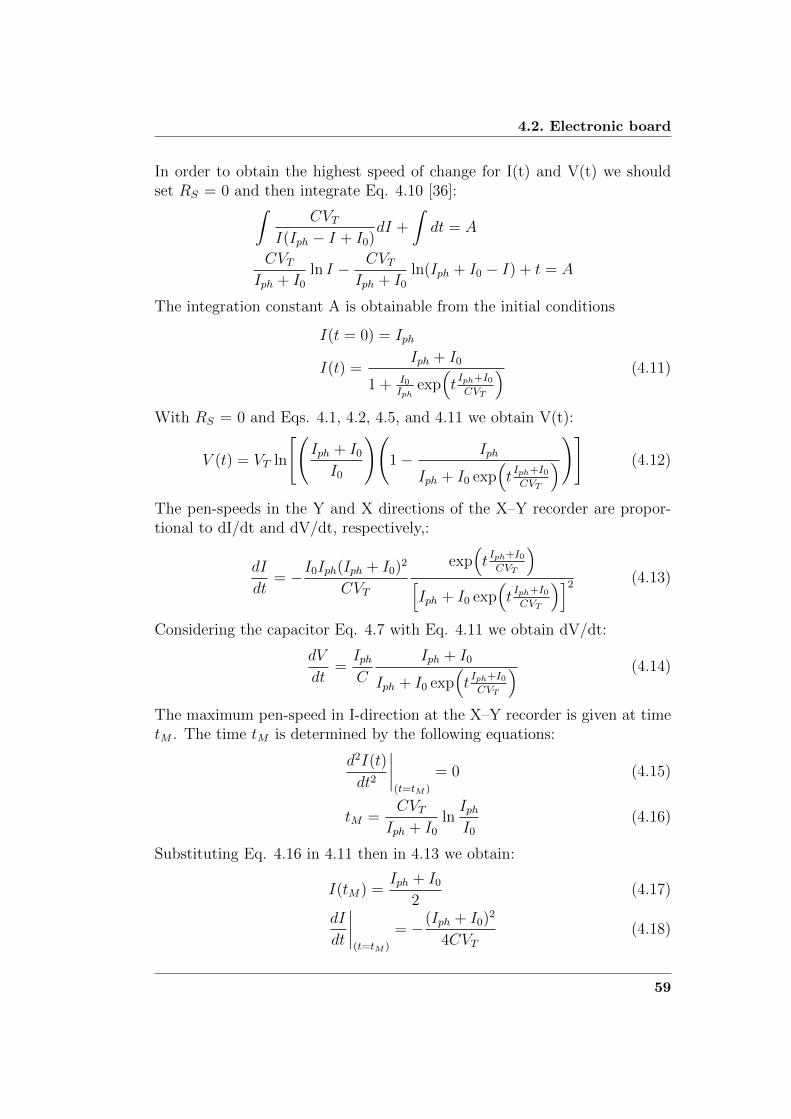
4.2. Electronic board
In order to obtain the highest speed of change for I(t) and V(t) we shouldset RS = 0 and then integrate Eq. 4.10 [36]:∫
CVTI(Iph − I + I0)
dI +
∫dt = A
CVTIph + I0
ln I − CVTIph + I0
ln(Iph + I0 − I) + t = A
The integration constant A is obtainable from the initial conditions
I(t = 0) = Iph
I(t) =Iph + I0
1 + I0Iph
exp(tIph+I0CVT
) (4.11)
With RS = 0 and Eqs. 4.1, 4.2, 4.5, and 4.11 we obtain V(t):
V (t) = VT ln
[(Iph + I0I0
)(1− Iph
Iph + I0 exp(tIph+I0CVT
))] (4.12)
The pen-speeds in the Y and X directions of the X–Y recorder are propor-tional to dI/dt and dV/dt, respectively,:
dI
dt= −I0Iph(Iph + I0)
2
CVT
exp(tIph+I0CVT
)[Iph + I0 exp
(tIph+I0CVT
)]2 (4.13)
Considering the capacitor Eq. 4.7 with Eq. 4.11 we obtain dV/dt:
dV
dt=IphC
Iph + I0
Iph + I0 exp(tIph+I0CVT
) (4.14)
The maximum pen-speed in I-direction at the X–Y recorder is given at timetM . The time tM is determined by the following equations:
d2I(t)
dt2
∣∣∣∣(t=tM )
= 0 (4.15)
tM =CVT
Iph + I0lnIphI0
(4.16)
Substituting Eq. 4.16 in 4.11 then in 4.13 we obtain:
I(tM) =Iph + I0
2(4.17)
dI
dt
∣∣∣∣(t=tM )
= −(Iph + I0)2
4CVT(4.18)
59

Chapter 4. Design of the experimental apparatus for LILTmeasurements
The maximum pen-speed in V-direction at the X–Y recorder is given at timet = 0. Substituting this value in Eqs. 4.12 and 4.14.
V (0) = 0 (4.19)
dV
dt
∣∣∣∣t=0
=IphC
(4.20)
At t=0, V(0)=0 and the short circuit current (Isc) of the PV generator flowsin the capacitor; setting t=0 in Eq. 4.11 we obtain
I(0) = Iph ≈ Isc (4.21)
At t=∞ the capacitor C will be fully charged. Substituting t=∞ in Eq.4.12, we obtain the open circuit voltage (Voc) of the PV generator:
Voc = VT lnIph + I0I0
(4.22)
Since Iph I0 and Iph ≈ Isc, Eq. 4.22 will be
VT =Voc
ln IscI0
(4.23)
Setting this value in Eq. 4.16, with Iph = Isc in Eq. 4.17, 4.18 and 4.20 weobtain:
tM = CVocIsc
(4.24)
I(tM) =Isc2
(4.25)∣∣∣∣dIdt∣∣∣∣(t=tM )
= − I2sc4CVT
(4.26)
dV
dt
∣∣∣∣t=0,V (0)=0
=IscC
(4.27)
The charging process of the capacitor is assumed to last tS (settling time)when I(t) ≈ I0 and, with Eq. 4.23, we obtain tS:
tS = 2CVocIsc
(4.28)
or
C =ts2
IscVoc
(4.29)
Therefore, the capacitor size is directly and indirectly proportional to theshort circuit and open circuit voltage of the PV generator, respectively. Fur-thermore, the higher the speed of the measuring system, the smaller will bethe size of the required capacitor [38].
60

4.2. Electronic board
4.2.2 Description of the board
In the Figures 4.6 and 4.7 are reported the pictures of the electronic boardand in Table 4.1 all components utilized.
Figure 4.6: Pictures of the first part of the electronic board.
In the following subsection are reported the layout of the principal compo-nents that permit to the electronic board to work, all the description referto the pictures mentioned above.The solar cell is attached at the terminals numbered with 1 (there are twoentrance for “+” and two for “-”), the positive pole is under the cell andthe negative are the two small tongues situated on the top of the cell, in theboard the positive is signed with a “+”.The board is fed with two different voltages attached at the component num-bered with 2 (the components with numbers from 1 to 5 and 7 are in theFigure 4.6, numbers from 6 to 9 are in Figure 4.7), a voltage of 5.07 is at-tached at “+” mark and a voltage of -0.44 is connected to the “-” sign, allthe ground cable going into “m” mark (not visible in the figure).At the terminal 3 are attached the cable that measured the voltage and thecurrent of the cell, and send all the measures to a matlab file trough the1208FS-USB device.It’s important to note that there are different switches in the board. Theswitch with the number 4 positioned in the part with one point “•” indicates
61

Chapter 4. Design of the experimental apparatus for LILTmeasurements
Figure 4.7: Pictures of the second part of the electronic board.
that only one amplifier for the current is in function, in the case that theswitch is on two points “••” indicates that one more amplifier is in function.When the position of this switch is changed the power that feeds the elec-tronic board must be turned off.The switches at point 5 are to decide what resistance to insert for the gain ofthe second amplifier, portrayed below. The switches at point 6 in the secondboard are to decide what capacitor to use, it is possible to use more thanone.The two boards are connected trough a bridge cable signed with number 7for all two boards and trough a bridge cable for the power supply of 5.07,from the terminal at point 2 in first board to the terminal at point 9 in thesecond board.In the terminal numbered with 8 arrives the cable from the 1208FS-USBdevices that commands the relays of the board.In Figure 4.8 it is reported the sketch of function of the electronic board.At the begin there is the photovoltaic solar cell, that is attached with thered cable at the positive and black cable at the negative. In parallel there isattached an operational amplifier that amplify the values of voltage of theo-retical 5 times. At a later stage there are two operational amplifier (Figure4.9) positioned in series at the extremity of a resistance. This element is
62

4.2. Electronic board
Table 4.1: List of components used for the electronic board.
Component Quantities Specifications
Amplifier 3 AD 8853Resistance 2 100 KΩ
3 301 Ω1 40.2 KΩ1 3.92 KΩ1 475 KΩ1 909 KΩ1 18.2 KΩ1 16.5 KΩ1 14 KΩ
Capacitor 1 1 F2 0.68 F2 0.047 F3 0.1 µF2 1200 pF1 79.3 pF1 10 µF
Ceramic disc Capacitor 2 1.2 nFRadial silveredmica Capacitor 3 100 pF
1 1000 pF1 82 pF
Radial tantalum Capacitor 1 1 µFNon-polar electrolytic SU 1 10 µFRelay photovoltaic 3 PVN012APbFUltra Low Noise, PrecisionVoltage Reference
1 ISL21090
Logical buffer 1Jumper switch 8
important for changing the current in voltage, after that the first amplifiergives amplification of theoretical 706, the second amplifier can be made infunction with the switch positioned on two points ••; in this case a more am-plify is in function, the values can be decided on the basis of the resistanceinserted.
63

Chapter 4. Design of the experimental apparatus for LILTmeasurements
Figure 4.8: Sketch of the scheme of the electronic board.
Figure 4.9: Sketch of the two operational amplifier for the current.
The gain of an operational amplify is given by the resistances used:
G = 2R2
R1
64

4.2. Electronic board
In this case the resistance R2 (in the Figure 4.9 is named R6) is fixed at 100kΩ, the resistance R1 (in Figure 4.9 is R5) con be inserted trough a switch,in Table 4.2 are reported the values of the resistances with the respectivegain of the operational amplifier:
Table 4.2: Resistances that can be inserted in the second amplifier of thecurrent and respective gain of the operational amplifier.
Value of resistance R1 [kΩ] Gain of the amplifier
200 1100 218.2 10.9816.5 12.1214 14.28
After the amplifiers there are two relays in parallel. The “Short CircuitRelay” when is closed cut the rest of the circuit and permits to all the currentto pass to this part. The “Relay” when closed permits at the current togo in the capacitor, whereas the “Discharge Relay” permits at the variableresistance to be inserted in the circuit. How this relays work is described inthe subsection 4.2.3.
4.2.3 Software for data acquisition
The management of the data acquisition and the commands is done by theUSB-1208FS and it is interfaced with the “data acquisition toolbox” of mat-lab (Simulink). To start the data acquisition it is necessary to run the matlabfile “data acquisition”, this permits Simulink to start the simulation for col-lecting all data. In Simulink there are two blocks that command the USB,one is a digital output that commands the three relay of the circuit: Dis-charge Relay, Relay and Short Circuit Relay, as shown in Figure 4.8, thesecond is an analog input block that receives the values of voltage and cur-rent.In the Figure 4.11 it is possible to see the diagram that manage the relays.In principle there is a clock that manages the time, the switches that managethe relays are activated at different time.At the beginning all the relays are open. At time 1 the system closes the“Discharge Relay”, in this way the configuration permits to the capacitor todischarge trough the resistance insert in parallel with the capacitor. At time2 the “Short Circuit Relay” is closed; at this moment all the current passes
65

Chapter 4. Design of the experimental apparatus for LILTmeasurements
Figure 4.10: Pictures of the experimental apparatus in laboratory for testingthe electronic board.
trough this line. At time 3 the last Relay is closed with no consequenceson the circuit. At time 4 the “Discharge Relay” would be opened in orderto permit to the current to charge the capacitor when at time 5 the “ShortCircuit Relay” would be opened. From time 5 to time 10 happens the chargeof the capacitor, then the simulation finishes.For all the simulation the program collects all the data, but to recreate the I-V characteristic it is important to consider only the data when the capacitorbegins to charge till the end of the simulation.
4.2.4 Characterization of the operational amplifier
The operational amplifiers were chosen to work at precise values of gain,unfortunately the value of gain is different from the theory.Initially, 4 operational amplifiers were taken. These were soldered at the basewith a soldering iron tip at 300°C, these are named: A, B, C and D. Later,cause the values were strange, other four operational amplifiers were taken,three of them were soldered with hot-air welding and pasta at 300°C, becauseit was thought that the type of welding could be a cause of the problems,them were named: E, F and G. The last amplifier, named H, was solderedas the first four.
66

4.2. Electronic board
Figure 4.11: Blocks in Simulink file for the management of the relays of theelectronic board.
Figure 4.12: Blocks in Simulink file for the acquisition of the values of voltageand current.
To verify the effective gain, a test was made for the voltage and one for thecurrent.As said in subsection 4.2.2 the gain for an amplifier is given by the relationbetween the resistances, that is:
G = 2R2
R1
For the voltage R2 is 100 kΩ and R1 40.2 kΩ that make a gain of 4.975,whereas for the first amplifier of the current R2 is 1384 kΩ and R1 is 3.92
67

Chapter 4. Design of the experimental apparatus for LILTmeasurements
kΩ, so the gain is 706.12.For the voltage were tested all the amplifiers to verify if all them work in thesame mode.For this verification it was taken a generator of voltage and used in placeof the cell, then the circuit was powered with a voltage of 5.07 and -0.44 topermit at the operational amplifier to work. The value of the generator waschanged from zero to 1 Volt with small intervals, and these were the Vin.With a multimeter the values of voltage after the operational amplifier wereregistered, named Vout, these values are in the range of -2.5 and +2.5, thatis the range of working of the schedule, for calculation the gain this valuesare adjusted with the addition of +2.5.To calculate the gain for the voltage the following formula was utilized:
G =(Vout + 2.5)− Vref
Vin
where Vref is a value of voltage, that can be addicted in the operational am-plifier, for have the exit voltage in a range required.Following are reported the values for the calculation of the gain for the am-plifier A (Table 4.3) and E (Table 4.4).With this result it is possible to note that the values of gain are around thevalue of 5 expected, only the firsts numbers are slightly lower.For the fact that all the operational amplifiers worked in similar mode, it wasdecided that, for characterization the gain for the current, is necessary to useonly two amplifiers: one when is used only one amplification and two whenthere is an other amplification, but to compare the results in the second casethe gain of the second amplifier is one.Initially the circuit was made in short circuit condition, in this mode the cur-rent is at his maximum, so at Isc, and the voltage is null. In this conditionis possible to calculate the gain with the following formula:
G =IoutIin
where Iin is the current generated from a generator of current from 0 to 7 Aand changed in Volts with a resistance, Iout is the voltage after the gain.Observing this result, Table 4.6 with only one amplifier and Table 4.5 withtwo, it is immediately evident that for values of current under 200 mA thegain is not constant and significantly under the theoretical value. From200 mA to 700 mA the gain remain around 700, that is little less than 706theoretical. In the second case the values of gain are a little less than in thefirst, but remain the strange trend of the curve. To mark this problem theresults are inserted in a graph (see Figure 4.13), in that is possible to read
68

4.2. Electronic board
Table 4.3: Calculation of the gain for the voltage with the operational am-plifier “A”, the theoretical gain is 5.
Vout [V] Vout+2.5 [V] Vin [V] Vref [V] G error %
-2.482 0.018 0.004 0 4.286-2.233 0.267 0.054 0 4.944 -13.323-1.984 0.516 0.104 0 4.971 -0.536-1.732 0.768 0.154 0 4.987 -0.319-1.481 1.019 0.204 0 4.995 -0.162-1.230 1.270 0.254 0 5.000 -0.098-0.981 1.519 0.303 0 5.013 -0.263-0.731 1.769 0.354 0 4.997 0.321-0.481 2.019 0.404 0 4.998 -0.007-0.230 2.270 0.454 0 5.000 -0.0500.018 2.518 0.504 0 4.996 0.0790.283 2.783 0.554 0 5.023 -0.5460.541 3.041 0.604 0 5.035 -0.2240.809 3.309 0.654 0 5.060 -0.4911.065 3.565 0.704 0 5.064 -0.0851.341 3.841 0.754 0 5.094 -0.5941.597 4.097 0.804 0 5.096 -0.0321.832 4.332 0.854 0 5.073 0.4572.056 4.556 0.904 0 5.040 0.6502.270 4.770 0.954 0 5.000 0.7962.425 4.925 0.994 0 4.955 0.9142.452 4.952 1.000 0 4.952 0.055
the gain in function of the current for both cases.To understand this problem the technical support of the Analog Device wascontacted, from this exchange of emails was identify some possible causes ofthis problem were identified:
• The operational amplifier is very small, for this reason the resistancesand capacitors used must be very small (in dimension).
• The components attached symmetrical must have symmetrical lengthof cables.
• The components must be soldered near the operational amplifier, thepresence of cable can be given losses and interferences.
69

Chapter 4. Design of the experimental apparatus for LILTmeasurements
Table 4.4: Calculation of the gain for the voltage with the operational am-plifier “E”, the theoretical gain is 5.
Vout [V] Vout+2.5 [V] Vin [V] Vref [V] G error %
-2.482 0.018 0.004 0 4.286-2.234 0.266 0.054 0 4.926 -12.997-1.984 0.516 0.104 0 4.971 -0.909-1.732 0.768 0.154 0 4.984 -0.267-1.482 1.018 0.204 0 4.992 -0.145-1.231 1.270 0.254 0 4.998 -0.127-0.982 1.518 0.304 0 4.996 0.033-0.731 1.769 0.354 0 4.997 -0.005-0.481 2.019 0.404 0 4.997 -0.008-0.231 2.269 0.454 0 4.997 0.0020.017 2.517 0.504 0 4.994 0.0650.266 2.766 0.554 0 4.993 0.0170.516 3.016 0.604 0 4.993 0.0050.763 3.263 0.654 0 4.989 0.0651.011 3.511 0.704 0 4.987 0.0421.263 3.763 0.754 0 4.991 -0.0701.522 4.022 0.804 0 5.002 -0.2351.778 4.278 0.854 0 5.009 -0.1372.027 4.527 0.904 0 5.008 0.0322.253 4.753 0.954 0 4.982 0.5132.424 4.924 0.994 0 4.954 0.5742.467 4.967 1.000 0 4.967 -0.267
Searching to solve this problem it was taken the first amplifier for the current(in Figure 4.6 is the amplifier in middle), and the principal resistances wassoldered directly to the amplifier. Unfortunately, this change did not lead toany improvement.
70

4.2. Electronic board
Table 4.5: Calculation of the gain for the current with two operational am-plifier insert, the first with a theoretical gain of 706, the second a theoreticalgain of 1.
Iout [A] Iin [V] Iin [mA] G1
0.039 0.099 9.92 393.1450.140 0.243 24.3 574.0740.217 0.353 35.3 614.7310.325 0.504 50.44 643.5370.388 0.594 59.35 652.9910.457 0.693 69.26 659.8330.530 0.797 79.7 664.9940.608 0.907 90.68 670.1590.695 1.030 102.96 675.0190.700 1.036 103.6 675.6760.755 1.118 111.8 675.3130.989 1.457 145.7 678.4491.411 2.045 204.5 689.9761.688 2.442 244.2 691.2371.925 2.774 277.4 693.9442.115 3.044 304.4 694.8092.418 3.472 347.2 696.4292.715 3.891 389.1 697.7642.835 4.064 406.37 697.6403.052 4.364 436.44 699.2943.645 5.204 520.4 700.4234.315 6.162 616.2 700.2604.716 6.730 673 700.7435.053 7.266 726.6 695.445
71

Chapter 4. Design of the experimental apparatus for LILTmeasurements
Table 4.6: Calculation of the gain for the current with only one operationalamplifier insert, with a theoretical gain of 706.
Iout [A] Iin [V] Iin [mA] G2
0.041 0.095 9.5 431.5790.121 0.208 20.8 581.7310.188 0.303 30.3 620.4620.333 0.508 50.8 655.5120.393 0.593 59.3 662.2260.454 0.681 68.13 665.6390.535 0.795 79.48 672.4960.615 0.907 90.7 677.6190.699 1.027 102.7 681.0130.687 1.009 100.87 681.0750.757 1.109 110.9 682.5970.956 1.390 139 687.7701.403 2.020 202 694.5541.719 2.470 247 695.9511.925 2.763 276.3 696.7062.151 3.083 308.3 697.6972.367 3.390 339 698.2302.666 3.815 381.5 698.8202.848 4.070 407 699.7543.066 4.380 438 700.0003.667 5.232 523.2 700.8794.315 6.155 615.45 701.1134.693 6.687 668.7 701.8094.923 7.013 701.3 701.982
72

4.2. Electronic board
Figure 4.13: Graph of the current in mA and respective gain, G1 is with onlyone operational amplifier, G2 with two operational amplifier, in both casesthe theoretical gain must be 706.
73

Chapter 5
Tests
5.1 State of test
5.1.1 Tests carried out
The solar cells on the Philae lander were submitted to different tests ofcharacterization, experimental and numerical, which were mainly carried outby the Politecnico di Milano, the Officine Galileo (now selex Galileo) and theESTEC (European Space Research and Technology Centre). The resultsobtained by the Officine Galileo and by the ESTEC are described in theAlenia report. All the tests were carried out at BOL. Indeed, the data forthe EOL were obtained using the test carried out on Rosetta orbiter solarcells at EOL by INTA (Instituto Nacional de Tecnica Aeroespacial).
5.1.2 Alenia report
In the Alenia reports are the results of the tests carried out during the man-ufacturing of 6 panels. The tests were carried out by Officine Galileo andESTEC, the first, however, has only used single flash, while the second singleand multiple flash. In both cases, the tests were done in a laboratory envi-ronment, at a temperature of +25°C and at the solar constant of 1 and 0.11.The tests of Galileo have been made in different phases: after manufacturingand after thermal vacuum chamber; while those of ESTEC have been madebefore and after acoustic noise.These tests show that the Philae solar array complies all requirements ateach tested condition. The panel Wall 2 is an exception since it seems tohave degradations in the Vmax and Imax in the first test on the acoustic noisehowever the Pmax remains constant. These tests are given in the documententitled Alenia SD0646 “Hood solar panels test” [24].

5.1. State of test
The document SD0621 ”Rosetta Lander Solar Array Design Report” [25] de-scribes the tests performed by Officine Galileo on 6 panels at 0.11 SC, +20°Cand -80°C. It also compares results from Officine Galileo with those providedby INTA.Another remarkable document is the SP00000852 “Solar array simulator sup-port software” [26], which results from Galileo’s studies. This documentis the manual for the software that simulates the behaviour of the panels.The simulator has the following input: the radiation dose from 0 to 6.4 in10× 1014 e cm−2, the temperature from -150 to +50 °C, the solar constantfrom 0 to 1, the direction angle of latitude alpha from -180° to +180°, theangle beta (which defines the direction of longitude ) from 0° to 90°, and thenumber of damaged strings for each section from 0 to 2. Is important to notethat the software has a good accuracy for values at BOL at environmentaltemperature (error less than 1%), but so far it has not been validated withdata from a space mission.
5.1.3 Test made by Politecnico di Milano
The tests were carried out by Stefano Brambillasca in 2009 as part of histhesis “Celle solari per missioni verso corpi celesti lontani dal sole” [1]; theywere performed in LILT condition at CESI (Centro Elettrotecnico Sperimen-tale Italiano).Such tests were made on 10 cells approved by the Max Planck Institut furSonnensystemforschung as appropriate to the mission (“good for flight”)They were carried out at BOL; a first test was done at a temperature of+25°C at 1 and 0.1 SC, then tests were performed at 0.1 SC and by varyingthe temperature from +25°C to -120°C with intervals of 10°C between 0 and100 and intervals of 5°C between 100 and 120.
5.1.4 Test made by INTA
Most of tests made by INTA have been carried out on the Rosetta orbitercells which indeed are larger than the cells of the lander: 23,39 cm2 versus10,92 cm2 of Philae. The performed tests are shown in Table 5.1.Using data from the cells of the orbiter at EOL were obtained, by applying
certain formulas, data at EOL for the cells of the lander.
5.1.5 Tests to be made
In the document “Remaining questions regarding Rosetta Philae solar gen-erator” [31] Dr. J. Biele from DLR mentions some tests that could done by
75
Chapter 5. Tests
Table 5.1: Characteristics of the tests made on the orbiter and on the landerof Rosetta at INTA
Orbiter (cells area 23,39 cm2)
SC Temp(°C) Fluence (10× 1014 e cm−2)
1 from +25 to +150 from 0 to 90.03 from -155 to +25 from 0 to 90.11 +25 00.11 from -130 to +25 3.2 and 6.4
Lander (cell area 10,92 cm2)
SC Temp(°C) Fluence (1× 10¹⁴ e cm−2)
0.11 +25 0
PoliMi in the future; he suggests to remeasure cells at BOL, and after irradi-ation of the cells measure the values at EOL (but with a wire mesh filter torecheck the TC at BOL) , to record the IV curve in detail (512 points) andto measure the IV curve at low intensity 0.0121 SC with 2 filters 0.11.Other tests to be performed are those envisaging the partial coverage (shad-owing) of cells and panels to analyse their respective behaviour at EOL.These tests are crucial since during the landing on the comet there is a riskof dust or ice deposition on the panels.
5.2 Dark current characterisation
As mentioned in the Chapter 2, the relationship between the current andthe voltage of a solar cell can be illustraed on a graph. Figure 5.1 showsthat the position of the curve depends on the intensity of illumination; ifthere is no illumination, the cell is in situation of dark current so that thecurve in the first quadrant overlaps with the X axis, while the graph in thesecond quadrant is flat and suddenly grows exponentially, forming the socalled “knee”.
5.2.1 Experiment on Philae solar cell
The reverse characterization of the cells is critically important to face theproblem of shadowing. In fact, the Philae solar cells can reach the voltage
76

5.2. Dark current characterisation
Table 5.2: Summarizing table of the documents
Document S.C. Temp. °C Fluence Note
Solar hood pan-els test report
0.11 and 1 +25 BOL test on all pan-els after manu-facturing
Solar hood pan-els test report
0.11 and 1 +25 BOL test on allpanels afterthermal vacuumchamber
Solar hood pan-els test report
0.11 and 1 +25 BOL test on all pan-els after acousticnoise
Rosetta Landersolar array de-sign report
0.11 -80 e +20 BOL test on all panels
Report on LILTMEASURE-MENTS ofphilae solar cells
0.11 and 1 +25 BOL test on 10 cells
Report on LILTMEASURE-MENTS ofphilae solar cells
0.11 0–120 BOL test on 10 cells
Solar array unitdescription Issdraft
0.11 and 1 25 BOL test on all panels
Solar array sim-ulator supportsoftware
0-1 -150-+50 0-6.4x10¹⁴e/cm2
program for sim-ulations
of 7 V (the value of the voltage depends on the current, the temperatureand the solar intensity), however, in dark condition a solar cell reaches only−6/− 8 V. Given that there are eleven cells in a string, some problems mayoccur when ten of them are illuminated and only one is in shadow, since inthis case the resulting voltage is zero.The Figure 5.2 reports the reverse dark characterisation for philae solar cellsas described in the lander user manual [29]; according to the table the ab-solute breakdown voltage VB increases with the increase of the temperature,
77

Chapter 5. Tests
which indicates breakdown by the avalanche mechanism [22].The lander user manual gives the following formula for the nearly linearhigh-current portion (50− 200 mA) of the reverse I-V dark curve:
Vreversedark(I, t) = −(7.63+2.4I)−(0.00485+0.0031I)t+(6.4·10−6−1.0·10−4I)t2
where I is in Ampere, V in Volt, t in °C.
5.2.2 Experiment made at Polimi
The experiments reported by LUM were carried out with strings of 1 or 9cells in a thermal chamber and different temperatures were tested: +60°C,
Figure 5.1: Terminal I–V characteristics under full, partial, and zero illumi-nations.
Figure 5.2: Reverse (dark) I-V characteristics for different temperaturespresent in LUM. Irev in mA, Urev in V [29].
78

5.2. Dark current characterisation
+20°C, 0°C and -60°C. In the graphs showing their results the characteristiccurves have been normalized to 1 cell.The experiments at the Polimi were repeated using only one cell (the numberof the cell is L012203) in the thermal vacuum chamber and the temperaturesof: +23.2°C, −0.3°C and −20.1°C. For the temperature of 23.2°C the experi-ments were performed with and without vacuum, for the other temperaturesthey were made only with vacuum conditions.The temperature values which were choosen for the experiments are the meantemperature of each point of the curve. For the first point of the curve, whenthe current is zero, the temperature remains constant; instead, by increasingthe cell voltage the intensity of the current also increases thus causing a cellheating; for the last point of the curve, the increase of the temperature isaround +14 in the first case and +6.5 in the cold case.During the experiment the cell in the chamber is connected with a cable to agenerator of voltage, starting with a voltage of zero Volt and increasing withintervals of 0.5 Volt until -5 Volt; subsequently the intervals are of 0.2 untilreaching -8 Volt; after this value are only considered the points at −8.1 and−8.15 Volt (but not for the cold case).
Figure 5.3: Reverse (dark) I-V characteristics for different temperatures inthermal vacuum chamber at the Polimi. I in mA, V in V.
79

Chapter 5. Tests
Figure 5.4: The cell in the thermal vacuum chamber.
5.2.3 Consideration
By observing the chart of the results obtained at Polimi (Figure 5.3, it isinteresting to observe that the values of the first linear part are the same forall trials, and that for the first trial the values with and without vacuum areapproximately the same. When comparing the two experiments, from thePolimi and from the LUM it appears that in both cases the curve becomesprogressively narrower with the cooling of the cell; moreover the knee of thecurve is situate in the same position, between -7 and -8 Volt.Taken together, it is possible to conclude that the results obtained at Polimiare consistent with the values presented by the LUM.
5.3 Laboratory conditions test
For testing the validity of the electronic board different tests at different val-ues of solar intensity hare been made. For the illumination of the solar cellit is taken a small incandescent lamp, changing the distance from the cell itis possible to obtain different values of intensity.Below are reported the results for a test made with the cell number L012203.All the test is monitored with the aid of two multimeters, in this mode ispossible to know the Isc, that in this case is 35.1 mA, and the Voc, for this
80

5.3. Laboratory conditions test
case is 0.527 V.At the end of the simulation the program shows four different graph.The first is the graph of the voltage versus the time (Figure 5.5); it can beseen that at time 5.5 s the electronic board begins to charge the capacitors.
0 1 2 3 4 5 6 7 8 9 10−1.6
−1.4
−1.2
−1
−0.8
−0.6
−0.4
−0.2
0
0.2
T [s]
V
Tension in function of time
Figure 5.5: Voltage in function of time for the test made on a cell at ambientconditions.
The second is the current in function of time, in Figure 5.6, in this graph itcan be seen that many points are out of the trend of the graph, caused byproblems of disturbance.The third graph that the program gives is the I-V curve (Figure 5.7), takenfrom the values of the former two graphs beginning from the time of 5 s, butin this case the values are in the range of the usb device, that is between thevalues of −2.5 and +2.5.The last graph, Figure 5.8, is the I-V curve in the real scale; unfortunatelythe points of beginning of the graph (up left) aren’t at the value of zero, butare shifted to right, this is given by problems of resistance inside the cell andin the capacitor, but for the graph is not a big problem because the first partof the I-V curve is linear.Observing the results is immediately noticed that there are many interfer-ences and there isn’t a line but a lot of oscillations, this is caused probablyby the lamp, but there were not enough tests to determine the true cause ofthe problem.
81

Chapter 5. Tests
0 1 2 3 4 5 6 7 8 9 10−2.5
−2.45
−2.4
−2.35
−2.3
−2.25
T [s]
I
Current in function of time
Figure 5.6: Current in function of time for the test made on a cell at ambientconditions.
−1.6 −1.4 −1.2 −1 −0.8 −0.6 −0.4 −0.2 0 0.2−2.5
−2.45
−2.4
−2.35
−2.3
−2.25
V
I
I−V curve
Figure 5.7: Curve I-V for the test made on a cell at ambient conditions inthe values of scale of the usb device.
82

5.3. Laboratory conditions test
0 0.1 0.2 0.3 0.4 0.50
5
10
15
20
25
30
35
40
V [V]
I [m
A]
I−V curve
Figure 5.8: Curve I-V for the test made on a cell at ambient conditions.
83

Chapter 6
Conclusions
The objective pursued for the present work was to create an experimentalequipment for characterization of solar cells at low intensity and low temper-ature. At this scope was realized a cooling coil that permits the cell to reachtemperatures under -100°C and an electronic board that takes the valuesof current and voltage from the cells and sends all the data directly to thecomputer.The test made on the cooling coil showed that it doesn’t have leakage whenit is in function, that reaches low temperature rapidly, and that the cell mustbe in contact with the coil to have the same temperature measured. Onlysmall devices must be done; the first is to create a slot to permit to insert acable for the positive pole of the cell, the second is to find a system to adherewell the cell at the coil.The most problematic work was to create the electronic board. In the boardwere inserted different resistances and amplifiers for have different gains, butwith the test, it results that the operational amplifiers work in strange modefor the different values of current. An other problem found is in the capaci-tors for the charge: initially were inserted different capacitors with differentvalues that could be inserted or not in the circuit; but the problem of allcapacitors used is that all have a big resistance in series, and this doesn’tpermit to have a lot of point in the I-V curve for the first part, when thecapacitors begin to charge. For this reason it is necessary to replace this withcapacitors with a smaller resistance in series. Moreover with the equation4.29 is possible to have an idea of the value of the capacitor. The result fromthe test showed that there are a lot of interferences in the result, but thegraph shows the trend of a normal I-V curve. For this reason it is necessaryto make other tests and changes on the board to make it effective to itspurpose.

6.1. Future developments
6.1 Future developments
To recreate the final experimental apparatus there is still much work tobe done. Below are summarized the key points for the construction of theexperimental device and the tests to be performed:
• Design of the base plate and cooling coil: both are made in this thesis.
• Design of the electronic board: it is made in this thesis, but some testsmust be done to perform the perfect working of the electronic board,and the capacitors must be changed for have more points in the firstpart of the curve.
• Box for made the experiments: the box must have an exit for thecables and the pipe for the liquid nitrogen, but is necessary to designan entrance with gaseous nitrogen to not have problems of condensationon the cell. The upper face of the box must be transparent to permitthe solar lamp to illuminate the cell, the other walls is better if theyare dark for not have problems of interference. An other propertyto consider in the design is that the cell on the cooling coil must bechanged a lot of time.
• Solar lamp: is necessary that this lamp have different filter to makethe tests at different values of solar intensity.
• Tests at ambient conditions.
• Tests at LILT conditions at BOL: this test are important to confrontnew results with the existent results.
• Test at LILT conditions at EOL: it is possible to perform these testsafter artificially irradiation of the solar cells.
• Tests whit a partial shadowing.
• Test with the presence of dust.
85

List of acronyms andabbreviations
67P/CG 67P/Churyumov-GerasimenkoAM0 Air Mass 0AR AntireflectionASTM American Society for Testing and MaterialsAU Astronomical UnitBOL Begin of lifeCESI Centro Elettrotecnico Sperimentale ItalianoDLR Deutschen Zentrums fur Luft- und RaumfahrtEOL End of lifeESA European Space AgencyFSS First Science SequenceHST Hubble Space TelescopeLILT Low Intensity Low TemperatureLTS Long Term ScienceLUM Lander User ManualMLI Multi-layer insulationMPPT Maximum Power Point TrackerNASA National Aeronautics and Space AdministrationNTT New Technology TelescopePolimi Politecnico di MilanoRTG Radioisotopes Thermoelectric GeneratorSA Solar ArraySAS Solar Array SystemSC Solar ConstantSDL Separation, Descent, and LandingWMO World Meteorological Organization

Bibliography
[1] Stefano Brambillasca, Celle solari per missioni verso corpi celesti lontanidal Sole, Tesi di Laurea Politecnico di Milano, 2007/2008.
[2] Giulia Damonte, Analysis and characterization of Solar cells for missionto Jupiter, Tesi di Laurea Politecnico di Milano, 2005/2006.
[3] K.-H. Glassmeier, H. Boehnhardt, D. Koschny, et al., The Rosetta mis-sion: flying towards the origin of the solar system, Space Science Re-views, Springer, 2007.
[4] KM. Pesco and A. E. Finzi, Rosetta Space Mission - The Solar Ar-ray Photovoltaic Assembly, at XIX Congresso Nazionale AIDAA, Forlı- Italy, 2007.
[5] Hans S. Rauschenbach, Solar cell array design handbook, volume 1, Na-tional Aeronautics and Space Administration, Springer, 1976.
[6] European Space Agency, Rosetta mission, http://sci.esa.int/science-e/www/area/index.cfm?fareaid=13
[7] Wikipedia, The Free Encyclopedia, http://www.wikipedia.org
[8] Amazing Space, http://http://amazing-space.stsci.edu/
[9] P. Lamy, I. Toth, et al., A portrait of the nucleus of comet67p/Churyumov-Gerasimenko, Space Science Reviews, Springer, 2007.
[10] Bjorn J.R. Davidsson, Pedro J. Gutierrez, Nucleus properties of Comet67P/Churyumov–Gerasimenko estimated from non-gravitational forcemodeling, Icarus Vol. 176, Elsevier, 2005.
[11] Konrad J. Kossacki , Jacek Leliwa-Kopysty´nski, Slawomira Szutowicz,Evolution of depressions on Comet 67P/Churyumov–Gerasimenko: Roleof ice metamorphism, Icarus Vol. 184, Elsevier, 2006.

Bibliography
[12] Masateru Ishiguro, Cometary Dust Trail Associated with Rosetta Mis-sion Target:67P/Churyumov-Gerasimenko, Icarus , 2007.
[13] J. Agarwal, M. Muller, G. Eberhard, Dust environment modelling ofcomet 67P/Churyumov-Gerasimenko, Space Science Reviews Vol. 128,Springer, 2006.
[14] R. Schulz, J. A. Stuwe, H. Boehnhardt, Rosetta target comet67P/Churyumov-Gerasimenko, Postperihelion gas and dust productionrates, Astronomy & Astrophysics, Eso, 2004.
[15] Flavio Iurato, Ottimizzazione di celle solari al GaAs per missioni sullasuperficie di Marte, Tesi di Laurea Politecnico di Milano, 2003/2004.
[16] Giulio Pinzan, Landing Site Selection for Rosetta Lander Philae througha Multidisciplinary Approach, Tesi di Laurea Politecnico di Milano,2011/2012.
[17] Gianluca M. Caputo, On-comet attitude determination of Rosetta landerPhilae through nonlinear optimal system identification, Tesi di LaureaPolitecnico di Milano, 2011/2012.
[18] CESI, Solar cells achievements & road map for space and Earth, Seminarat Politecnico di Milano, 2012.
[19] C.J. Gerderloos, R.J. Walters, et al., Low Intensity Low TemperaturePerformance of Advanced Solar Cells, IEEE, 2002.
[20] H.Y. Tada, J.R. Carter, et al., Solar Cell Radiation handbook, NASA,JPL, 1982.
[21] Harold J. Hovel, Semiconductors and Semimetals, Vol. 11: Solar Cells,Academic Press, 1975.
[22] S. M. Sze, Physics of Semiconductor Devices, Wiley-Interscience, 1969.
[23] Mukund R. Patel, Spacecraft power systems, CRC Press, 2005.
[24] Gwenael Beltrame, Luca Vallini, Solar hood panels test report, Alenia,2001.
[25] Gwenael Beltrame, Rosetta lander solar array design report, Alenia,2001.
[26] M. Barela, Solar array simulator support software, Galileo Avionica,2004.
88

Bibliography
[27] Gwenael Beltrame, Luca Vallini, Flight panels test plan and procedure,Alenia, 2001.
[28] Francesco Topputo, Report on LILT mesuraments of philae solar cells,Politecnico di Milano, 2007.
[29] J. Biele, Solar array unit description Iss draft, LUM, 2011.
[30] J. Biele and S. Ulamec, Capabilities of Philae, the Rosetta Lander, SpaceScience Review, vol. 138, pp. 275-289, 2008.
[31] J. Biele, Remaining questions regarding Rosetta PHILAE solar genera-tor, Comments after telecon with Gianfelice D’Accolti, 27.04.2012.
[32] J. Biele and S. Ulamec, From the Rosetta lander Philae to an asteroidhopper:lander concepts for small bodies missions, report and presenta-tion, German Aerospace Center (DLR), 2004.
[33] Imre Toth, What’s new about 67P/CG? - Characterization of the phys-ical properties of the nucleus of comet 67P/CG, 3rd Post-Launch work-shop of the Rosetta Philae Science Team, Konkoly Observatory Bu-dapest, 17 December 2007.
[34] Mahmoud Marwan, Ismail Naban, Analytical and graphical methods fordetermination of solar cell parameters and investigations of shadowingeffect, Int J Sol Energy, UK, vol. 9, pp. 179–192, 1990.
[35] L. Nashelsky, R. Boylestad, Electronic devices and circuit theory, 6thed. Englewood Cliffs, NJ: Prentice Hall, 1996.
[36] Mahmoud Marwan, Investigations on characteristic parameters andpower degradation of amorphous silicon solar modules based on long-term outdoor testing, International Energy Journal, Vol. 2 No. 2, De-cember 2001.
[37] DLR Rosetta Mission Brochure - Journey to a comet, Deutsches Zen-trum for Luft und Raumfahrt, 2008.
[38] Marwan M. Mahmoud, Transient analysis of a PV power generatorcharging a capacitor for measurement of the I–V characteristics, Re-newable Energy, vol. 31 (13) Elsevier, 2006.
[39] VV.AA., Rosetta Lander - System Status after Five Years in Space,Aerotecnica Vol.88, No.4, 2009.
89

Bibliography
[40] F. Topputo, F. Bernelli-Zazzera, F. Ercoli-Finzi, Solar Array Simulatorsfor Low Power Space Missions, Proceedings of the 3rd CEAS Air &Space Conference, 2011.
90