Design of a Linear High Precision Ultrasonic Motor

ABSTRACT

BAUER, MARKUS GEORG. Design of a Linear High Precision Ultrasonic

Piezoelectric Motor. (Under the direction of Dr. Thomas A.Dow.)

To understand the operating principles of linear ultrasonic piezoelectric motors, a motor

made by Nanomotion Ltd. was examined and a model of the driving process was

developed. A new motor has been designed that uses the same driving process but

improves resolution, speed, efficiency and especially controllability. All designs involve

at least two independently driven piezoelectric elements, one generating the normal load

at the interface and the second generating the tangential driving force. The greatest

challenges in developing this motor are 1) the actuator needs to have two different mode

shapes at nearly the same frequency and 2) each mode shape must be exclusively excited

by one actuator and not by the other. The quality of the operation of the motor directly

depends on how well the excitation of both vibrations can be separated.

Finite element analysis (FEA) has been used to model the actuator and predict the

dynamic properties of a future prototype. The model includes all significant features that

have to be considered such as the anisotropy of the piezoelectric material, the exact

properties and the dimensions of the actuators (including all joints). Several prototypes

have been built, and the resulting mode shapes and natural frequencies have been

measured and compared to the computer models. The design concepts as well as the

modeling techniques have been iteratively improved.

Open loop testing has shown that the motor generates slideway motion such that the

steady state slideway velocity is proportional to the excitation voltage. To fully

characterize the motor and to demonstrate its full potential for positioning tasks, the

motor has been tested in a closed loop control system. Despite saturation of the control

input and nonlinearities in dynamics of the motor-slideway system, it was shown that a

simple feedback control system using proportional gain or proportional-integrating

control algorithms can be used to achieve a stable responsive positioning system.

DESIGN OF A LINEAR HIGH PRECISION

ULTRASONIC PIEZOELECTRIC MOTOR

by

MARKUS G. BAUER

A dissertation submitted to the Graduate Faculty of

North Carolina State University

in partial fulfillment of the

requirements for the degree of

Doctor of Philosophy

MECHANICAL ENGINEERING

Raleigh

2001

APPROVED BY:

ii

BIOGRAPHY

Markus Georg Bauer was born in Remscheid, Germany. He received his Master's degree

in mechanical engineering (Diplom-Ingenieur) in March 1998 at RWTH-Aachen

(University of Aachen, Germany). For his Master's thesis, he designed a computer-

controlled robotic manipulator arm using piezoelectric actuators to control joint

impedance and incremental angular encoders for position feedback.

He is currently pursuing a Ph.D. degree in mechanical engineering and is employed as a

research assistant at the precision engineering center in Raleigh, North Carolina.

iii

ACKNOWLEDGEMENTS

I would like to thank the following people for their advice, support and friendship

throughout the course of my graduate work at the PEC.

Very special thanks to my dear wife Myriam. Without her I would have never found the

PEC and missed many things. Thanks for all the love and support you gave me during

the last three years and for helping me make full sentences out of all these green and red

words.

Dr Dow for being my advisor and for providing a challenging and fascinating project in

an excellent environment in which to conduct research, for his guidance and for his belief

in my ability to solve all the many small and big problems which I encountered during

my research.

Drs. Richard Keltie, Ron Scattergood and Paul Ro for teaching excellent courses and for

serving on my committee.

Burleigh Instruments for inspiring this project and for their financial support of the PEC.

Alex, Wendy, Ena, Cathy, Laura for doing their part to make the PEC a great place and

especially Ken for solving so many of my computer problems and providing inside into

the PC31 card when Innovative Integration did not.

All my friends and fellow students at the PEC, for their friendship, many lunches and

discussions: Bradley (for orienting me to the PEC), Byoung (for being an inspiration and

for contributing to the 20 lb. weight gain at the Bean Sprout), Daran, David (for home-

cooked meals enjoyed until after 9 p.m., and for relieving me of seminar duty), Edd (for

teaching me how an American should be), Eddi, Matias (for his encouragement--we

made it, man!), Matt, Mike, Nobu (for continuing the PEC lunchtime tradition) and

Wonbo.

iv

TABLE OF CONTENTS

LIST OF TABLES ........................................................................................................vii

LIST OF FIGURES......................................................................................................viii

LIST OF SYMBOLS AND ABBREVIATIONS ............................................................ xi

1 Introduction.............................................................................................................1

1.1 Precision Actuators ..........................................................................................1

1.2 Ultrasonic Motors ............................................................................................3

1.2.1 Travelling Wave Motors ..........................................................................4

1.2.2 Standing Wave Motors.............................................................................6

1.3 Actuator Materials ......................................................................................... 10

1.3.1 Piezoelectric Actuators........................................................................... 10

1.3.1.1 The Piezoelectric Effect ..................................................................... 11

1.3.1.2 PZT Materials for Ultrasonic Motors.................................................. 13

1.3.1.3 Actuator Types................................................................................... 14

1.3.2 Electrostriction....................................................................................... 14

1.3.3 Magnetostriction .................................................................................... 16

2 Ultrasonic Standing Wave Motors ......................................................................... 20

2.1 Driving Process for Standing Wave Motors ................................................... 21

2.2 The Nanomotion Motor ................................................................................. 23

2.2.1 Motor Specifications .............................................................................. 24

2.2.2 Measurements of Force and Motion ....................................................... 25

2.2.3 Limitations of the Nanomotion Motor .................................................... 28

2.3 Model of the Driving Process......................................................................... 29

2.3.1 Equation of Motion ................................................................................ 29

2.3.2 Limitations of the Model ........................................................................ 31

2.3.3 Model Verification................................................................................. 31

2.4 Requirements for the New Motor Design ....................................................... 34

3 Actuator Design..................................................................................................... 36

3.1 Vibration Analysis ......................................................................................... 37

3.1.1 Analytical Methods ................................................................................ 40

3.1.2 Numerical Analysis................................................................................ 41

v

3.1.2.1 ANSYS .............................................................................................. 42

3.1.2.2 Boundary Conditions.......................................................................... 42

3.2 Vibration Measurements ................................................................................ 43

3.2.1 Piezoelectric Force Sensor ..................................................................... 45

3.2.2 Optical Displacement Sensor.................................................................. 45

3.3 Prototypes...................................................................................................... 46

3.3.1 L-shaped Prototype ................................................................................ 46

3.3.2 T-shaped Prototype ................................................................................ 50

3.3.2.1 Experimental Results.......................................................................... 51

3.3.2.2 Thermal Effects.................................................................................. 53

3.3.3 I-shaped Prototypes................................................................................ 55

3.3.3.1 Actuator Excitation and Resonances................................................... 57

3.3.3.2 Motor Performance ............................................................................ 58

3.3.4 I+ Prototype ............................................................................................ 59

3.3.4.1 Actuator Design ................................................................................. 59

3.3.4.2 Actuator Construction ........................................................................ 60

3.3.4.3 Actuator Excitation and Resonances................................................... 62

3.3.4.4 Motor Support.................................................................................... 63

3.3.4.5 Open Loop Motor Performance .......................................................... 65

4 Closed Loop Position Control................................................................................ 68

4.1 System Setup ................................................................................................. 69

4.1.1 Computer-Motor Interface...................................................................... 70

4.1.1.1 Motor Excitation ................................................................................ 71

4.1.1.2 Position Feedback .............................................................................. 73

4.2 System Analysis ............................................................................................ 73

4.2.1 Transfer Functions ................................................................................. 73

4.2.2 Stability ................................................................................................. 75

4.2.3 Steady State Accuracy............................................................................ 78

4.3 Controller Implementation ............................................................................. 81

4.4 Closed Loop System Response ...................................................................... 83

4.4.1 P-Control ............................................................................................... 83

vi

4.4.2 PID-Control ........................................................................................... 85

4.4.3 Gain Scheduling PID Controller............................................................. 87

4.4.4 Control Parameters................................................................................. 90

4.5 Closed Loop Performance Summary.............................................................. 90

5 Conclusion ............................................................................................................ 92

5.1 Driving Process ............................................................................................. 92

5.2 Actuator Design............................................................................................. 93

5.3 Closed Loop Position Control ........................................................................ 95

5.4 Future Research ............................................................................................. 96

REFERENCES ............................................................................................................. 98

Appendix A - Piezoelectric Materials .......................................................................... 101

Appendix B - Sliding Friction ..................................................................................... 105

Friction Measurement Apparatus ......................................................................... 106

Friction Measurements ........................................................................................ 107

Results................................................................................................................. 109

Appendix C – Solving the Equation of Motion for the Slideway.................................. 110

Appendix D - Optical Displacement Sensor................................................................. 114

Appendix E – Brief Description of the Design of an FEA Model................................. 116

Appendix F – Calculated Mode Shapes for the L, T, I and I+ prototypes ...................... 118

Appendix G - Prototype Manufacturing and Assembly (I+ Prototype).......................... 124

Appendix H – General Design Considerations............................................................. 128

Appendix I - Circuit Diagram of the Computer-Motor Interface .................................. 131

Appendix J – Source Code for the Control Program .................................................... 135

vii

LIST OF TABLES

Table 1.1: Properties of Soft PZT and Hard PZT ........................................................... 13

Table 2.1. Specifications of the Motor [7] .................................................................... 25

Table 4.1: Summarized Gain and Phase Margins........................................................... 77

viii

LIST OF FIGURES

Figure 1.1: Driving Process of Travelling Wave Motors..................................................4

Figure 1.2: Ring-type Travelling Wave Motor, Used in Canon Autofocus Lenses ...........6

Figure 1.3: Ultrasonically driven standing wave motor ....................................................7

Figure 1.4: Standing Wave Motors by Kumada (left) and Bein (right) .............................8

Figure 1.5: Motor by Nanomotion Ltd.[6] .......................................................................9

Figure 1.6: The Inverse Piezoelectric Effect. ................................................................. 11

Figure 1.7: Polarization of Piezoelectric Ceramics [11] ................................................. 12

Figure 1.8: Electrostrictive Strain vs. Electric Field (Material: PMN-15) [11]................ 15

Figure 1.9: Joule Magnetostriction Caused by Application of a Magnetic Field [13]...... 17

Figure 1.10: Magnetostriction, Basic Mechanism [13]................................................... 17

Figure 2.1: Motion of the Motor Tip for Different Phase Angles ................................... 21

Figure 2.2: Photograph of the Nanomotion Motor ......................................................... 23

Figure 2.3: Nanomotion Motor, Mode Shapes [6].......................................................... 24

Figure 2.4: Slideway Velocity for Constant Excitation (Nanomotion Motor) ................. 26

Figure 2.5: Excitation Voltage vs. Slideway Velocity (Nanomotion Motor)................... 27

Figure 2.6: Equation of Motion for the Slideway ........................................................... 30

Figure 2.7: Slideway Velocity for maximum Motor Excitation...................................... 32

Figure 2.8: Theoretical Effect of Changes in the Thrust Force ....................................... 33

Figure 2.9: Theoretical Effect of Changes the Phase between the Thrust Force and the

Normal Force ........................................................................................................ 34

Figure 3.1: Modal Participation ..................................................................................... 38

Figure 3.2: Mass-Spring Model (a) and Continuos Beam in Bending (b) of a Rectangular

Actuator ................................................................................................................ 41

Figure 3.3: Mode Shape Measurements ......................................................................... 44

Figure 3.4: Optical Displacement Sensor....................................................................... 46

Figure 3.5: L-Shaped Prototype..................................................................................... 47

Figure 3.6: Mode Shape Measurement of the L-shaped Prototype ................................. 49

Figure 3.7: T-shaped Prototype ..................................................................................... 50

Figure 3.8: Force Measurement, ±100V Excitation........................................................ 52

Figure 3.9: Temperature Measurement .......................................................................... 53

ix

Figure 3.10: I-shaped Prototype..................................................................................... 56

Figure 3.11: Mode-Shapes with Corresponding Resonant Frequencies .......................... 58

Figure 3.12: I+ Prototype ............................................................................................... 60

Figure 3.13: Composition of the I+ Actuator .................................................................. 61

Figure 3.14: Motor Support ........................................................................................... 64

Figure 3.15: Slideway Velocity for Different Excitation Voltages ................................. 66

Figure 3.16: Steady-State Slideway Velocity................................................................. 66

Figure 4.1: Photograph of the Motor-Slideway System.................................................. 68

Figure 4.2: Block Diagram of the Closed Loop System ................................................. 69

Figure 4.3: Schematic of the Computer-Motor Interface ................................................ 71

Figure 4.4: Bode plot of the linearized transfer functions GM0.5, GM

2.5, GM5.0 ( Equation

(4.5 – (4.7) ) 76

Figure 4.5: Simplified Block Diagram of Closed Loop System...................................... 79

Figure 4.6: System Response to a Step Input Using P-feedback Control (Kp=0.15)........ 84

Figure 4.7: Steady-State Position Error Using P-control (KP=0.15)................................ 85

Figure 4.8: Closed Loop PI-control Measured and Simulated System Response ............ 86

Figure 4.9: SIMULINK Model ...................................................................................... 87

Figure 4.10: System Response using a Gain scheduling PID Control (KP=0.15,

KI=1,KD=0.02)....................................................................................................... 88

Figure 4.11: Position Error Using a Gain Scheduling PID Control................................. 89

Figure A.1: Piezo-Kinetics Material Datasheet ............................................................ 104

Figure B.1: Experimental Setup................................................................................... 106

Figure B.2: Simplified Model of the Experiment ......................................................... 107

Figure B.3: Measured Friction Forces vs. Sliding Velocity for Different Excitation

Frequencies, Normal Force = 8.2N.............................................................................. 108

Figure D.1: Calibration curve for the optical displacement sensor ............................... 114

Figure F.1: Resonance f10=44.826kHz ......................................................................... 118


Figure F.3: Resonance f3=39.543kHz .......................................................................... 119

Figure F4: Resonance f4=43.979kHz ........................................................................... 120

Figure F5: Resonance f4=52.633kHz ........................................................................... 120

x





Figure F.10: Resonance f3=41.275kHz ........................................................................ 123

Figure G.1: Actuator components................................................................................ 126

Figure G.2: Cut the Actuator Shape Step 1 .................................................................. 126



Figure I.1: Circuit Plan of the Computer – Motor Interface.......................................... 131

Figure I.2: Schematic of a Second Order Low Pass Filter ............................................ 132

Figure I.3: Filter Transfer Function for R1=2.2kΩ, R2=888Ω, R3=1.4kΩ, C1=10nF,

C2=1.2nF .................................................................................................................... 134

xi

LIST OF SYMBOLS AND ABBREVIATIONS

∆l ............................................................................................................. Length change

∆W .........................................................................................Energy dissipated per cycle

( )δtan ............................................................................... Loss factor (material damping)

ε ............................................................................................................Mechanical strain

η ......................................................................................................................Loss factor

ϕ, ϕ0 ............................................................... Phase between tip motion and normal force

ϕM ................................................................................................................ Phase margin

µ .....................................Coefficient of friction between the tip and the slideway surface

ω, ω* .....................................................................Circular frequency (in radians/second)

C(s) ................................................................Position input function (in Laplace domain)

D.............................................................................................Controller transfer function

D(s)..................................................... Controller transfer function in the Laplace domain

D(z)................................................................Controller transfer function in the z-domain

E ....................................................................................... Young’s modulus, electric field

ek ...................................................................... Discrete position error in the time domain

E(s) ...........................................................................Position error in the Laplace domain

esteady-state .................................................................................... Steady-state position error

F ..........................................................................Amplitude of the dynamic normal force

f ....................................................................................................frequency in Hz or kHz

F0 ................................................................................................................. Preload force

FF ................................................................................................................ Friction force

FThrust ............................................................................................. Thrust force (at the tip)

FTip,N ............... Normal force at the motor tip caused by the longitudinal actuator vibration

FN, Fnormal ...................................................Normal force (relative to the slideway surface)

GCL .......................................................................................Closed loop transfer function

GM ................ Transfer function of the motor-slideway system (includes power amplifiers)

gM...................................................................................................................Gain margin

xii

H.............................................................................................................Magnetic field H

k ................................................................................. Index in the discrete control system

KC......................................................................................................................................................................................Slope of the ramp input

KD ............................................................................................................. Derivative gain

KI .................................................................................................................. Integral gain

KP........................................................................................................... Proportional gain

L ........................................................................................................................... Length

m...................................................................................................... Mass of the slideway

Q....................................................................... Quality factor (=η1

for low damping loss)

T ..............................................................................................Sampling rate (in seconds)

uk.........................................................................Discrete controller output (time domain)

u(s)....................................................................... Controller output in the laplace domain

U ..........................................................................................................................Voltage

U*............................................................................................................................................................................................Linearization voltage

U(s)..................................................................ExcitationvVoltage in the Laplace domain

×v .................................................Steady state slideway velocity (for constant excitation)

vmin .......................................................... Smallest increment in the velocity measurement

W.........................................................................The total vibration energy in the system

x .........................................................................Direction, coordinate of slideway motion

x& .......................................................................................................... Slideway velocity

x&& .................................................................................................... Slideway acceleration

X(s) .................................................................... Slideway position in the Laplace domain

x(t) ............................................ Coordinate of slideway (in direction of slideway motion)

y ......................................................................................................................... Direction

z ....................................................................................Direction, time delay in z-domain

z& ................................................................Velocity of the tip motion in sliding direction

z0 .........................................................................................Amplitude of the tip-vibration

z(t) .......................................... Coordinate of tip motion (in direction of slideway motion)

xiii

FEA ...............................................................................................Finite element analysis

P-controller ............................................................................ Proportional gain controller

PI-controller .............................................................. Proportional Integral gain controller

PID-controller .......................................... Proportional Integral Derivative gain controller

PZT........................................................ Lead Zirconate Tiatanate (piezoelectric ceramic)

PMN .................................................... Lead-Magnesium-Niobate (piezoelectric ceramic)

1 INTRODUCTION

1.1 Precision Actuators

The demand for high precision positioning has grown rapidly in different fields ranging

from biology to machining. Positioning systems needed for many high technology

applications must satisfy an ever-increasing demand for high resolution and accuracy,

quick response time as well as high acceleration and high velocity. Precision actuators

are currently used in applications that require resolution and accuracy in the sub-micron

range; in the near future, this requirement will be in the sub-nanometer range. In terms of

precision, linear actuators have improved in position accuracy from tens of micrometers

in the 1920-1930's to tens of nanometers in the 1980-1990's. Early in the 21st century,

position accuracy of linear actuators is expected to be less than 1 nm [1].

Electromagnetic AC, DC and stepper motors are commonly used for simple positioning

tasks that do not require high resolution and accuracy [2]. Rotational electromagnetic

motors are easily available in almost any size from a few watts to several kilowatts. To

convert rotational motion into linear motion or to increase the resolution for high

precision actuation systems, different types of transmissions can be used. One possible

way to realize precise positioning over a long range of motion would be to use a DC

motor followed by a ball screw drive that is attached to a linear slideway [2]. For normal

and precision positioning accuracy, these actuators are generally preferred because of

their high stiffness, high output force, long range, and low cost. The resolution and

accuracy of ball and lead screw drives are usually limited by the resolution of motors that

are used to drive them, the backlash between the screw and threaded drive, and the non-

linearities of friction forces such as the slip-stick phenomenon. For slightly better

accuracy, higher performance ball screw drives and hydraulic actuators have been

developed with sub-micron accuracy and nanometer resolution. For sub-nanometer

accuracy and resolution, devices using piezoelectric materials have been developed.

2

For applications that require a range of motion on the order of 10 µm, actuators made

from active materials [1], such as piezoelectric materials, can be used. Positioning of the

object of interest is achieved by the deformation of the active material, which is linearly

dependent upon an applied voltage. Therefore, the displacement has an infinitely high

resolution (theoretically). The resolution is limited more by the device which supplies

the signal, such as a control system or an amplifier, than by the hysteresis of the material

itself. Advantages of such actuators using active materials include high stiffness, high

strength, and small size [1].

One technique to achieve long range motion and still exploit the advantages of active

materials requires a structure with multiple actuators. One of the first designs to generate

linear, long-range motion was the Burleigh Inchworm®, developed in the 1970's by

Burleigh Instruments. This design is centered around a single piezoelectric extension

element that has a piezoelectric clamping elements at each end. The three elements work

together to move the center rod. The clamps act as brakes that alternately grip and

release the rod while the extension element moves the rod. By proper synchronization of

the extension and clamp elements, linear motion is achieved. However, since the design

uses a single extension element, motion must pause during the retraction of the extension

element. This produces the characteristic stop and go motion associated with inchworm

type motors.

To achieve constant velocity with an inchworm type motor, the design and control

algorithms were modified by A. D. Ruxton [3] and J. C. Fasick[1] at the PEC. As a

continuation of the PEC concept, Burleigh Instruments designed and prototyped a

mechanism, the Inchworm® II, with two pairs of extension and clamping piezoelectric

actuators. The discontinuous clamping and unclamping can excite resonant frequencies

of the mechanism itself and those of attached structures and limit the speed capability.

Testing of both the PEC and Burleigh mechanism revealed a disturbance (a discontinuous

step) in the motion during each clamp change [1]. The velocity was limited by the

resonance frequencies of the extension actuator, the clamps and the stroke of the

extension actuator. While Inchworm type actuators provide high open loop positioning

3

resolution (and up to 20nm closed loop resolution using appropriate feedback sensors),

the maximum velocity is limited to about 2mm/s. The average lifetime travel is about

2000m. Applications that require a longer lifetime or a higher velocity require a different

solution.

1.2 Ultrasonic Motors

The development of ultrasonic motors has led to a new actuator type that has many

attractive properties for precision positioning tasks. Ultrasonic motors use mechanical

vibrations to produce a cyclic friction based driving force between one stationary and one

moving component.

Unlike electromagnetic motors, ultrasonic motors generate an electromagnetic field no

larger than a capacitor. They operate using electric fields, which means that they can be

used in environments where electromagnetic fields are not permitted. Ultrasonic motors

can be used directly for precise positioning without the need for gears or other

transmissions in linear or rotary drives. Because the driving process is based on friction,

most ultrasonic motors automatically maintain their position when the power source is

turned off. On the other hand, the wear associated with the frictional contact can

potentially lead to problems. The major disadvantage of this technology is the power

required to generate the high frequency vibration. For most designs a high-voltage high-

frequency power source is needed to drive the motor. For the motor to be efficient,

power amplifiers have to be designed to match the operating conditions and the electrical

properties of the motor. The nature of the active materials used to build the actuator in

combination with the need to operate at frequencies above 20kHz limit the motor’s size

and makes it difficult to design efficient amplifiers.

Ultrasonic motors can be used for positioning application that require small actuators

with high resolution. They are suitable actuators for robots, especially miniaturized

devices as well as actuators for the use in space and consumer goods such as camera

lenses. Canon introduced the first auto-focus camera lens that uses an ultrasonic motor in

4

1987 [4]). Depending on the specific design, ultrasonic motors have velocities up to 1m/s

(with the potential to be even faster) and a resolution below 1µm.

Discussion of the driving process requires that motors be classified into two main types:

travelling wave motors and standing wave motors. Both the process by which ultrasonic

motors generate slideway motion and the process by which travelling waves or standing

waves are excited in the motor are different for each type. Further differentiation, by

kind of vibrational mode, order of resonant modes, shape of the actuator, the active

material, the direction of motion generated (linear, rotary) affects more specific details of

the individual design than operating principle.

1.2.1 Travelling Wave Motors

Figure 1.1: Driving Process of Travelling Wave Motors

5

Travelling wave motors make use of the fact that if travelling waves propagate through

an overall stationary elastic beam, the particles on its surface undergo elliptical motion.

This process is illustrated in Figure 1.1. Material in the mid-surface of the beam does not

move in x-direction. The preload between movable and stationary motor component

provides frictional contact around the anti-nodes of the wave. The motion of the

travelling wave causes the location of the contact areas to change with the wave

propagation. To illustrate how a travelling wave in an overall stationary beam can be

used to produce motion, the trajectory of a surface particle has to be observed: At time 1

in Figure 1.1 the surface particle is just on the right of the contact area. Later, at time 2,

the wave has propagated such that the same surface particle has moved to the center of

the contact area. At time 3 the surface particle is about to leave the contact area. The

motion of the surface particle on the elastic beam as shown in Figure 1.1 illustrates how

the travelling wave generates a thrust force, which acts in opposite direction as the

propagation of the travelling wave. The path of the surface element as sketched in Figure

1.1 demonstrates why “elliptical displacement motion” is commonly used to explain the

operation principle of ultrasonic motors [4]. Note that only the surface motion within the

contact area affects the movable body. A standing wave would only move the particles

straight up and down in y-direction and as a result provide neither motion nor friction

force in x-direction. The velocity of a travelling motor is directly proportional to the

propagation velocity of the travelling wave and the distance between the neutral plane of

the beam and the surface that contacts the rotor.

The first working prototype of a travelling wave type ultrasonic motor was built and

tested by T. Sashida in 1982 [4]. The first successful commercial application followed

in 1987 when Canon introduced an autofocus lens that was driven by a ring shaped

travelling wave type ultrasonic motor, shown in Figure 1.2.

6

Figure 1.2: Ring-type Travelling Wave Motor, Used in Canon Autofocus Lenses

Piezoelectric elements excite a travelling wave in the stator. The teeth in the stator

increase flexibility and amplifies the motion of contact surface. The rotor is equipped

with a flexible flange to provide continuous contact around the ring without

compromising the circumferential rigidity. This motor offers a maximum velocity of 40

revolutions per minute (150mm/s surface circumferential velocity), 35% power efficiency

(max) and a maximum power of 0.8W.

1.2.2 Standing Wave Motors

The first ultrasonic standing wave motor was proposed by H.V.Barth in 1973 [4]. A rotor

is driven by pressing a piezoelectric ”Horn” against it, as illustrated in Figure 1.3.

7

Figure 1.3: Ultrasonically driven standing wave motor

Elongation of the piezoelectric element causes a force normal to the rotor surface. This

force causes the piezoelectric element to bend, which results in a thrust force that moves

the rotor. For clockwise rotation the vibrator on the left is used, for counterclockwise

rotation, only the vibrator on the right is excited. Although this principle had been

proven to work, there have not been any reports of an application using this motor [4].

In contrast to travelling wave motors where the moving object rides on the “crest” of a

number of waves, standing wave motors require only a single point of contact between

motor and moved object. “Elliptical displacement motion”, as commonly used in the

discussion of travelling wave motors, is present at the contact point, but since there is

only a single contact point, it remains in contact through the entire path of the motion.

The motor slides back and forth along the surface of the slideway while the vibration

normal to the sliding surface provides a variable normal force. This combination creates

a friction based driving force between one stationary component, the motor, and the slide

to be moved.

A wide variety of ultrasonic standing wave motors have been proposed. A motor by

Kumada [4], as shown in Figure 1.4 a) uses a single lagrangian-type actuator. The

actuator consists of a piezoelectric disk that is mounted (and preloaded) between two

8

large cylinders. The stiffness of the piezoelectric disk and the preload in combination

with the mass of the cylinders determines the natural frequency at which the actuator is

operated. A slot in the end cap, which is not in line with the ridge on top of it, causes the

end cap to twist when the longitudinal actuator vibration compresses it. This design

enables a single actuator to cause elliptical displacement motion and thus drives the rotor

Figure 1.4: Standing Wave Motors by Kumada (left) and Bein (right)

A different motor developed by Bein [5] (Figure 1.4 b) uses the fourth bending mode and

the first longitudinal mode to generate linear motion with up to 160mm/s velocity and

0.25N force (see Figure 1.4). The motor consists of a steel base that has thin layers of

piezoelectric material to excite the desired vibration. Excitation of the outer piezoelectric

elements predominantly excites the fourth bending mode, which causes actuator motion

in slideway direction between motor and slideway. The excitation of the actuator in the

center of the actuator primarily excites the first longitudinal vibration mode of the

actuator. The unsymmetrical design leads to secondary excitation of the first bending

9

(along with the fist longitudinal mode), which generates the vertical component of the

“elliptical displacement motion” required to generate slideway motion.

The only standing wave motor that is commercially available is made by Nanomotion

Ltd. [6]. This motor, as shown in Figure 1.5, uses a combination of a flexural and a

longitudinal vibration of a rectangular block of piezoelectric material to impose a

sinusoidal driving force on a linear or rotational stage.

Figure 1.5: Motor by Nanomotion Ltd.[6]

Excitation of electrode sections 1 and 4 excites the second bending mode and the first

longitudinal mode at a certain phase relationship. To change direction, electrode sections

2 and 4 are excited and the bending motion of the actuator is reversed. The excitation

frequency is constant at 39.6 kHz. This is called “velocity mode”. For fine positioning

this motor uses a different mode of operation: the "stepping mode". In stepping mode, a

saw-tooth voltage is applied to either pair of electrode sections, which makes the actuator

move slowly in one direction, while maintaining static friction, and then retract quickly.

The force applied by the sudden retraction and the inertia of the system overcomes the

static friction and initiates sliding between motor and slideway. According to the user

manual [7], the motor reaches a maximum velocity of 250mm/s and a resolution “better

than 100nm” in stepping mode.

10

1.3 Actuator Materials

The development of ultrasonic motors is closely associated with the availability of active

material to efficiently generate high frequency vibrations within an elastic body. Most

ultrasonic travelling wave motors are designed using a metal beam or disk that is excited

by thin layers of active material. If the active material is thin compared to the entire

actuator, its properties will not influence the dynamic behavior of the actuator

considerably and thus can be neglected for the most part of the design process. However,

for the design of standing wave motors, it is beneficial to use actuators that consist almost

entirely of the active material. Then, the vibrating medium must be stiff enough to allow

resonant vibrations in the ultrasonic range (above 20kHz). Its dynamic behavior

(resulting mainly from stiffness, density and damping losses) must also be known to

model the actuator dynamics.

Active actuator materials that use the piezoelectric effect are most commonly used in

ultrasonic motors. Recent progress in the development of electrostrictive and

magnetostrictive materials encourages the use of those materials for the design of

ultrasonic motors.

1.3.1 Piezoelectric Actuators

The piezoelectric effect was first observed on tourmaline crystals by the brothers Pierre

and Jacques Curie in 1880. The phenomenon of electrical polarization of crystals caused

by deformation in certain directions, was later given the name “piezoelectricity” by

Hankel. In 1881, Pierre and Jacques Curie proved experimentally the reverse action of

the piezoelectric effect, namely the mechanical deformation of crystals due to an applied

electric field. Simultaneously, the piezoelectric effect was discovered in a number of

other crystals, like quartz, zinc blende and Rochelle salt (tartaric acid) [8]. Today,

11

common piezoelectric ceramics are Lead Zirconate Titanates (PZT), Barium Titanate and

Lead Nickel Niobate materials.

1.3.1.1 The Piezoelectric Effect

In nonconductors (dielectrics), as opposed to conductors, electrons cannot move through

the material in the presence of electric fields. However, for a number of materials there is

an unbalance of electric polarization on a microscopic level, so to speak, a certain

displacement of positive and negative charges within the body. These are commonly

called dipoles. When most of these dipoles are oriented in the same direction, which

does not need to coincide with the electric field, the dielectric is ”polarized” on a

macroscopic level. When mechanical strain is applied to the material, the dipoles will

deform and the electrical equilibrium will change, which results in an electrical field on a

macroscopic level. This is called the piezoelectric effect. When an electric field is

applied in polarization direction, each dipole experiences an electric force, which cause

strain: the positive end of the dipole is pulled towards the negative electrode and vice

verse. This is called the inverse piezoelectric effect, which is sketched in Figure 1.6.

Figure 1.6: The Inverse Piezoelectric Effect.

12

Consequently, any non-conducting material that has oriented dipoles has piezoelectric

properties. Wood, for example, consists of oriented cellulose fibers that have dipole

characteristics. The piezoelectric strain of wood is in the same order of magnitude as

common piezoceramic materials [9]. Note that many polymers also have piezoelectric

properties if the polymer molecules are oriented during processing.

A lack of symmetry in the crystal structure is a requirement for monocrystalline materials

to have piezoelectric properties. This means that there is at least one axis in the crystal

where the atomic arrangement appears different if one proceeds in opposite directions

along it. For this reason, all piezoelectric crystals are anisotropic.

A polycrystalline material, when cooled below the Curie temperature in the absence of an

electric field, consists of many monocrystalline domains (Figure 1.7 on the left), all of

which have their individual microscopic polarization direction. Above the curie

temperature, the individual domains are able to flip to orient in the direction nearest to the

electric field, with the result that the crystal as a whole becomes an electric dipole. This

state is shown in Figure 1.7 on the right. Cooling the material to room temperature in the

presence of the electric field freezes the orientation of the individual dipoles. Within a

certain range of stress, which depends on the actual material, the variation of dipole

moment (~ electric field) with stress is approximately linear and reversible [10].

Figure 1.7: Polarization of Piezoelectric Ceramics [11]

13

Piezoelectric ceramics are the most commonly used piezoelectric materials. They are

polycrystalline materials with many randomly oriented domains. After firing, a ceramic

body is isotropic and exhibits no macroscopic piezoelectric effect. Components may be

made piezoelectric in any direction by a “poling treatment“ which involves exposing the

ceramic to a high electric field at temperature not far below the Curie temperature.

1.3.1.2 PZT Materials for Ultrasonic Motors

Today, piezoelectric ceramics (mostly PZT) are available from many different

manufacturers, who use a variety of processes to achieve certain material properties.

Generally PZT materials are divided into Soft and Hard PZTs. Their most important

properties relevant to the design of ultrasonic motors are compared in Table 1.1.

Table 1.1: Properties of Soft PZT and Hard PZT

Soft PZT Hard PZT Effect on:

Increased dielectric

constant

Decreased dielectric

constant

Actuator capacitance

( causes electric loss)

High dielectric loss Low dielectric loss Electric loss

Low mechanical Q (~50) High mechanical Q (~900) Resonance amplification

(High Q ~ low Damping)

Lower E-modulus Higher E-modulus Actuator stiffness

High strain coefficient Low strain coefficient Actuator stroke

The material of choice for the design of ultrasonic piezoelectric standing wave motors is

the family of Hard PZTs. The objective is to excite the actuators at one of the mechanical

resonances, which must be above 20kHz (to be ultrasonic). The actuator stroke is

amplified by the resonance effect, which increases with decreasing mechanical damping.

Although Hard PZTs have a much strain coefficient (smaller stroke), they exhibit lower

damping losses, increases the amplitude at resonance and also minimizes heat generation

in the actuator.

14

1.3.1.3 Actuator Types

Because piezoelectric materials require an electric field typically between 3000V/mm and

300V/mm and the largest strain is in direction of the electric field, actuators have been

developed that consist of a stack of parallel layers of piezoelectric material. The actuator

is made from a large number of thin layers (typically ~20µm) of piezoelectric material

which are separated by electrodes and glue layers. This small spacing of electrodes

allows the application of a strong electric field at low excitation voltages. If stacked

actuator with 20µm thick layers requires 60V to achieve maximal strain, a 3mm thick

piece of the same material requires 9000V to do the same. The orientation of the

electrodes allows the application of a strong electric field in the direction of primary

material strain, which makes stacked piezoelectric actuators a good solution for

applications that require a large static displacement. They cannot be operated near

resonance because the material experiences high internal stresses due to the mismatch in

stiffness between the different materials (piezoelectric ceramic, electrodes and glue)

within the composite structure. In addition, the large number of soft glue layers accounts

for high elastic damping losses that lower the resonance amplification and also cause an

increase the actuator temperature to the point where the glue fails.

Although the motor performance is directly proportional to the actuator strain, the use of

solid PZT material is highly recommended for the design of ultrasonic motors. The

benefits of Hard PZTs are lower dynamic stresses, lower damping and thus higher

resonance strain, which results in a more stable and more robust motor. In this

configuration, the electric field is orthogonal to intended strain direction and a higher

voltage is required to reach the nominal strain.

1.3.2 Electrostriction

The nature of the electrostrictive effect is very similar to the piezoelectric effect. While

the piezoelectric effect can be characterized by linear electromechanical coupling

15

(between stain and the electric field), electrostriction displays behavior of second-order

electromechanical coupling [12].

Piezoelectricity: ε = ≈ ⋅∆l

lconst E (1.1)

Electrostriction: ε = ≈ ⋅∆l

lconst E2 (1.2)

where: l: Length; ∆l : Length change; ε : mechanical strain; E: electric field

This means, that in electrostrictive materials the direction of the electric field does not

influence the strain. The effect is illustrated in Figure 1.8. Note that there is no inverse

electrostrictive effect: mechanical stress does not generate an electric field.

Figure 1.8: Electrostrictive Strain vs. Electric Field (Material: PMN-15) [11]

Electrostrictive materials based on PMN (lead-magnesium-niobate) crystals have recently

been developed that seem to show a performance in respect of strain and damping losses

which is similar to the most advanced PZTs. One potential benefit of this using

electrostrictive instead of piezoelectric materials could be that if the actuator is excited

with a symmetric AC voltage, the resulting mechanical vibration has twice the frequency

of the electrical excitation.

16

Both PZTs and PMN can be selected that have comparable Young’s modulus, density

and strength. Strain coefficients which are slightly larger that those of soft PZT, and a

Quality Factor Q, which is about as high as the one of hard PZTs make PMN based

materials look promising for the use in resonating actuators, i.e. ultrasonic motors. The

ability to double the frequency by using a symmetric excitation certainly is an advantage

when it comes to high-voltage high-frequency power amplifiers, because the because the

amplifier bandwidth can be half the frequency of the actuator vibration. On the other

hand, the in comparison to PZTs large dielectric coefficient accounts for 40-times higher

capacitive losses.

The main reason why PMN has not been used in the ultrasonic motors is that both the

material itself as well reliable data of material properties are not widely available. In

summary, the material is much more expensive than a suitable PZT. However, the

comparison to PZTs is difficult and exact modeling of the actuator dynamics is virtually

impossible without a complete list of material properties.

1.3.3 Magnetostriction

Magnetostriction can be described most generally as the deformation of a body in

response to a change in its magnetization (magnetic moment per unit volume). In other

words, a magnetostrictive material will change shape when it is subjected to a magnetic

field (Compare: Piezoelectric and electrostrictive materials change shape in an electric

field!). All magnetic materials exhibit magnetostriction to some degree. The highest

magnetostriction of a pure element is observed with Cobalt, which saturates at 60

microstrain. However, of technical significance are alloy materials that experience Giant

Magnetostriction (strains in the order of 0.2%). This effect occurs in a small number of

materials containing rare earth elements [13].

17

Figure 1.9: Joule Magnetostriction Caused by Application of a Magnetic Field [13].

The mechanism of magnetostriction at an atomic level is relatively complex subject. The

basic idea is that there are magnetic dipoles within the material. These dipole domains

have a certain magnetic orientation whereas the individual domains are oriented

randomly within the material. The magnetic dipoles orient in the direction of an applied

magnetic field H as shown in Figure 1.10. The material will elongate in direction of the

field and grow smaller in the other directions.

Figure 1.10: Magnetostriction, Basic Mechanism [13]

18

At the first glance, piezoelectric and magnetostrictive materials should be suitable for the

same applications that include sound and vibration sources, active damping elements,

vibrational (ultrasonic) motors, force and pressure sensors and linear high precision

actuators. The strain (~0.16%), Young’s modulus (~50GPa) density (~9000kg/m3), and

thus the wave speed in the material, should be very similar. If only the active material

were considered, the natural frequencies of a sensor or actuator would be similar

compared to piezoelectric materials. For applications that operate at low frequencies

(below 1kHz), magnetostrictive materials might even have advantages over piezoelectric

materials because their static strain is larger.

For use in resonators, especially standing wave motors, the magnification of the

amplitude at resonance is more important than the DC stroke, because near resonance the

system response is dominated by the mechanical loss factor (or Q-factor), which is lower

than suitable piezoelectric or electrostrictive materials.

The need to generate a magnetic field (and its implementation) is the main reason why

magnetostrictive materials are not a good alternative for ultrasonic motors:

• Electromagnets are heavy and require space. The additional mass of the coils,

required for magnetostriction, will decrease the natural frequency and thus the

bandwidth of the system (for other applications, the higher strain of magnetostrictive

materials could be of advantage).

• Strong magnetic fields are required to generate required strain. Eddy-currents and the

resistive and inductive losses of the coils cause most of the energy losses of

magnetostrictive actuators. Eddie currents also increase with frequency, which limits

the bandwidth to about 10kHz for currently available materials [13].

• Ultrasonic motors require several actuators that are very close to each other.

Magnetic fields must be contained to the volume of the intended actuator material and

must not influence any of the other actuators.

19

To this date piezoelectric materials have the general advantage of availability and price.

Because piezoelectric materials have been widely used for a much longer time, many

more different materials are commercially available. Piezoelectric materials are also

cheaper and all necessary material properties are available.

20

2 ULTRASONIC STANDING WAVE MOTORS

Piezoelectric motors that use travelling waves have been the subject of many publications

in recent years. These motors are commercially available (e.g. Canon’s autofocus drive)

and are suited for applications that require a fast response time, power-off holding

capabilities and high resolution without backlash. Whereas extensive research has been

conducted on piezoelectric travelling wave motors, very few successful piezoelectric

standing wave motors have been reported [4]. Compared to piezoelectric travelling wave

motors, standing wave motors generally have the advantage of a very simple and very

light mechanical design, and they can be used directly in linear or rotational drives.

Control related problems, which occur mainly while moving slowly or changing

direction, are an obstacle for precise positioning and have prevented widespread use to

date. To overcome those problems, a motor by Nanomotion Ltd., which is the only

commercially available piezoelectric standing wave motor, uses an additional fine

positioning mode.

This chapter begins by describing the driving process of standing wave motors. A

piezoelectric motor made by Nanomotion Ltd. is then presented as an example of a

commercially available standing wave motor, which was used to study the driving

process. By using the principles learned from this motor, an equation of motion for the

general driving process could be developed. The solution to this theoretical equation is

then compared to the measured velocity of the Nanomotion motor. The greatest benefit

of the model of the general driving process lies in the insight gained into the effects of

different parameters of the actuator vibration on the theoretical motor performance.

These are the basis for the design of the improved ultrasonic standing wave motor, which

is discussed in Chapter 3.

Before a strategy can be proposed to design an improved piezoelectric standing wave

motor that does not show the limitations of existing motors, the operating principle must

be fully understood. To accomplish this, the analysis of piezoelectric standing wave

motors can be separated into two domains: the motion of the tip and the effect of this

21

motion when it is loaded against a slideway. Motion normal to the sliding surface turns

into a dynamic normal force and motion in the sliding direction experiences sliding

friction, which creates a thrust force. It is essential to first understand how both

components of the oscillating tip motion interact to generate slideway motion.

Subsequently, an actuator needs to be designed that is capable of generating the required

tip motion.

2.1 Driving Process for Standing Wave Motors

The first step in understanding how standing wave motors work requires better

knowledge of how the oscillating motion of the motor tip generates slideway motion. To

accomplish this goal, the tip motion is examined more closely. The curves shown in

Figure 2.1 represent the motion of a single point at the end of the tip that is in contact

with the slideway surface.

Figure 2.1: Motion of the Motor Tip for Different Phase Angles

The tip motion is the product of a two-dimensional vibration at the interface between

motor tip and slideway. The motion in each direction can be represented with a

22

sinusoidal function. As the vibration in both directions has the same frequency, the phase

between them is constant. The amplitudes of each of the two components as well as the

phase between them are the three quantities that determine the shape of the curves as

shown in Figure 2.1. For simplicity the amplitudes are normalized. During operation,

the motor is preloaded against the slideway, such that the tip does not move away from

the slideway surface. The actuator vibration then causes strain in the actuator, which is

experienced as a normal force through the stiffness of the contact point. To generate

slideway motion, the motor tip slides back and forth along the slideway surface. Motor

and slideway interact via a friction-based force, which depends on the direction of

relative motion, the coefficient of friction and the magnitude of the normal force. The

inertia of the slideway is too large for the slideway to actually follow the motion of the

motor tip. However, the direction of the relative sliding velocity between tip and

slideway changes, which determines the direction of the friction force, which then

accelerates (and decelerates) the slideway in the respective direction. In order for the

reciprocating tip motion to generate continuous slideway motion, the average normal

force must be larger during the part of the cycle when the tip is sliding in the direction of

the desired slideway motion. The slideway is accelerated more during this part of the

cycle than it is decelerated when the tip retracts under the influence of a smaller than

average normal force.

The phase angle between the sliding motion and the normal force controls the time during

a cycle when the slideway is accelerated and decelerated, because the magnitude of the

dynamic normal force influences the amount of frictional force that is present in the

system. A relative phase angle of 90°, as drawn in Figure 2.1, means that the normal

force, and thus the friction force, is smaller than average when the tip moves from the left

to the right, resulting in a minimal acceleration in this direction. In this case, the friction

force at any time during the second part of the cycle is larger than during the first half,

meaning that the acceleration from the right to the left is at a maximum (for given

amplitudes). In addition, at a 90° phase angle, the maximal tip velocity coincides with

the maximal friction force. Smaller as well as larger phase angles result in a lesser

overall slideway acceleration, smaller maximum slideway velocity and lower motor

23

efficiency. A phase of 270° reverses the slideway direction. The tip motion has the same

shape as shown in Figure 2.1 for 90°, but the motion is in the opposite direction.

2.2 The Nanomotion Motor

The standing-wave motor produced by Nanomotion Ltd. [6], [7] is an example of a

motor that uses the driving process described in the preceding section. This motor was

used to study the general process by which slideway motion is produced in the velocity

mode. A photograph of the motor is shown in Figure 2.2. The preload spring presses the

motor to the right against the motor case. A ceramic tip is attached to the actuator and

transmits the forces from the actuator onto the object that is to be moved. When the

motor is loaded against a slideway, the preload spring is compressed further and the

actuator loses contact with the motor case. It is then supported only by two small steel

rollers on one side and two rubber pieces that allow horizontal motion in order to apply a

constant preload but constrain motor movement in the slideway direction (vertical as in

Figure 2.2). Motor motion in the slideway direction is generally undesirable, because it

allows the slideway to move independently from the motor excitation.

Figure 2.2: Photograph of the Nanomotion Motor

24

This motor uses the first longitudinal resonance of a rectangular-shaped piezoelectric

actuator to generate a sinusoidal normal force and the second bending resonance to

generate a force in the direction of motion. The actuator is made from a single block of

piezoelectric material, that has a common electrode on one side but on the opposite side

the electrode is divided into four sections. Excitation of electrode sections 14 and 20 (as

labeled in Figure 2.3) with a sinusoidal voltage at the operating frequency of 39.6kHz

results in slideway motion in one direction. Excitation of electrode sections 16 and 18

with the same voltage results in slideway motion in the opposite direction. The

amplitude of the excitation determines the velocity.

Figure 2.3: Nanomotion Motor, Mode Shapes [6]

2.2.1 Motor Specifications

Nanomotion Ltd. produces a number of piezoelectric motors with different specifications,

however all of them use the same actuator. The differences lie in the number of actuators

used in parallel. Multiple parallel actuators proportionally increase the driving force and

smooth the motor velocity by averaging the effects of multiple frictional contacts, which

minimizes the influence of individual disturbances. To obtain deeper understanding of

25

the operation of linear ultrasonic piezoelectric motors, the motor with a single actuator

(PCLM Series, Model SP-1), a matching amplifier and a high precision linear stage with

a range of 30 mm were obtained. The most important motor specifications, as supplied

by Nanomotion Ltd., are summarized in Table 2.1.

Table 2.1. Specifications of the Motor [7]

Maximum velocity (load dependent) 250 mm/s

Maximum force 5.3 N

Resolution (smallest step) 20 nm

Static holding force 9 N

Operational frequency 39.6 kHz

Maximum operating voltage 240 V

Maximum operating current (load dependent) 0.0875 A

Ambient operating temperature 0° to 50° C

2.2.2 Measurements of Force and Motion

Because both vibrations are forced upon the actuator at the same frequency, the combined

motion of the tip is dominated by this one frequency. The amplitude of the dynamic

normal force was measured to be ±12.5N using a piezoelectric force sensor. The force

sensor was mounted between the motor and ground. Alternatively, the dynamic normal

force at the tip can be estimated by measuring the longitudinal motion at the preload

spring.

With the assumption that the longitudinal motion within the actuator is symmetric with

respect to its center, the longitudinal motion at the tip is similar to the longitudinal motion

at the preload spring. Any influence of the stiffness of the tip-slideway contact on the

longitudinal mode shape is neglected in this case, which is a reasonable assumption since

the stiffness of the contact point is much less than the stiffness of the actuator material.

Both methods yield almost identical results.

26

The tip displacement caused by the bending vibration of the actuator is more difficult to

measure without changing the boundary conditions of the actuator vibration. However,

the bending displacement can be measured at a location between the end of the tip and

the motor support. Assuming both the actuator and the tip do not deform significantly

between the location of the measurement and the end of the tip, the amplitude of the end

of the tip can be estimated to about ±4 µm (for the maximum excitation voltage). As

already mentioned in Chapter 1, the Nanomotion motor reverses the direction of slideway

motion by exciting different regions of the actuator. Although the phase between

longitudinal and bending vibration of the actuator changes with the motor preload, this

change is not significant if the motor is set up correctly. Measurements showed that the

phase is between 70° and 110° or –70° and -110°, based on which electrodes are

activated (1 and 4 or 2 and 3).

Figure 2.4: Slideway Velocity for Constant Excitation (Nanomotion Motor)

Figure 2.4 shows the slideway velocity when an excitation with constant amplitude is

applied at the actuator. The motor is capable of accelerating a slideway with a mass of

27

2.28kg to a maximum velocity of 235mm/s in less than one second. To achieve the

maximum velocity, the preload has to be carefully adjusted while monitoring the

slideway speed. This behavior demonstrates how sensitive the motor is to changes in the

surface topography.

The smallest velocity, vmin, that can be computed from the position measurement of the

slideway is limited by the resolution of the encoder, which is 11.08_m and the data

collection rate (500Hz or once every 2ms). The smallest velocity is equal to the change

in position of one encoder increment from one measurement to the next. The resolution

of the velocity as shown in Figure 2.4 is given by:

s

mm

s

mv 54.5

002.0

08.11min ==

µ(2.1)

The steady state velocities for constant motor excitation from Figure 2.4 are plotted as a

function of the excitation voltage in Figure 2.5.

Figure 2.5: Excitation Voltage vs. Slideway Velocity (Nanomotion Motor)

28

The slideway does not move until the excitation voltage reaches about 150V, more than

half its maximum, because the thrust force at the motor tip must overcome static friction

(a result of the static preload) to allow relative motion between slideway and motor.

Once slideway motion is initiated, sliding friction replaces static friction at the motor-

slideway interface, which results in a sudden jump in the slideway velocity. Reducing

the excitation from its maximum also reduces the slideway velocity down to zero, which

changes the sliding fiction to static friction.

The steady state velocity of the Nanomotion motor is very sensitive with respect to the

motor preload. Please note the variations in the motor velocity in Figure 2.4. Small

changes in preload cause the steady state velocity to vary between about 230 and 260

mm/s. Lower excitation voltages lead to random transitions between static friction and

sliding friction, which was not considered in the model. An excitation of 140V (compare

to Figure 2.5) of the Nanomotion motor does not produce enough thrust force to

overcome static friction and thereby cannot move the slideway whereas actuator vibration

of any amplitude in the model predicts slideway motion

2.2.3 Limitations of the Nanomotion Motor

The major disadvantages of the Nanomotion motor are revealed in Figure 2.4 and Figure

2.5. These measurements also reveal the two major disadvantages of the Nanomotion

Motor:

1) The steady-state velocity is not very constant, especially at slow velocities. It seems to

be almost impossible to move slower than about 20mm/s at a constant excitation without

occasional standstill (Figure 2.4).

2) When the steady-state slideway from Figure 2.4 is directly compared with the

excitation voltage in Figure 2.5, it can be seen that the steady-state slideway velocity is

not proportional to the excitation voltage.

To change the direction of motion, a much larger change in excitation voltage is required

than to just increase or decrease slideway velocity in the same direction. In order to

29

obtain such different excitation voltages, the controller gain must be directly linked to the

slideway velocity and direction. Thus, a constant controller gain is likely to cause

instability. Both the hysteresis for small slideway velocities and the nonlinear response

to the control signal are great challenges for the design of a stable control algorithm with

reasonably fast response time and high resolution.

In addition to the stability problems at slow motor velocities mentioned in the previous

paragraph, the soft motor support, which is also different in each direction, allows the

slideway to move independently of the motor tip–slideway contact. This makes the

system sensitive to external disturbances.

2.3 Model of the Driving Process

The next step towards creating a motor which avoids some of the shortcomings of the

Nanomotion motor involved understanding the driving process. The equation of motion

was derived using the driving process as described in Chapter 2.1. The slideway velocity

predicted by the model can be verified by comparing it to the actual velocity of the

Nanomotion motor. These results then enabled determination of requirements for a new

motor design and helped to predict its performance

.

2.3.1 Equation of Motion

The amount of acceleration that is experienced by the slideway during each individual

cycle is relatively small considering maximum frictional forces on the order of 10N and

maximum actuator strokes around 2µm. However, the analysis of the Nanomotion motor

showed that repeating this cycle 40,000 times per second make it is possible to generate

slideway velocities on the order of 250mm/s. To verify the concept mentioned above and

to be able to analyze the influence of phase, sliding motion, normal force and preload on

the slideway motion, a model of this process had to be developed.

30

The model that was used to obtain the equation of motion for the slideway is shown in

Figure 2.6. The slideway (mass m and coordinate x) is accelerated by the friction force

FF. The direction of the friction force depends on the direction of the relative speed of

slideway and motor tip.

Figure 2.6: Equation of Motion for the Slideway

Case a) zx && > : ( ) ( )tFtxm Nµ−=&& (2.2)

Case b) zx && < : ( ) ( )tFtxm Nµ=&& (2.3)

Both cases combined: ( ) ( ) ( )[ ] ( )tFtztxsignumtxm N&&&& −= (2.4)

With: ( )tFFFN ωcos0 += (2.5)

( ) ( )00 sin ϕω −= tztz (2.6)

( ) ( )00 cos ϕωω −= tztz& (2.7)

Substituting equation (2.5) and (2.7) into (2.4) yields the complete equation of motion for

the slideway:

( ) ( ) ( )[ ] ( )( )tFFtztxsignumm

tx ?+−−= ωϕωωµ

coscos 000&&& (2.8)

31

x(t): coordinate of slideway (in direction of slideway motion)

z(t): coordinate of tip motion (in direction of slideway motion)

F0: preload force

F: amplitude of sinusoidal normal force, must not be larger than F0

z0: amplitude of tip-motion

ϕ0 : phase between tip motion and -force

m: mass of the slideway

µ : coefficient of friction between the tip and the slideway surface

An analysis of the friction between motor tip and slideway can be found in Appendix B.

The coefficient of friction, µ, for an alumina tip sliding on an alumina surface has a value

of 0.182 and does not depend on sliding velocity of excitation frequency.

2.3.2 Limitations of the Model

The two main assumptions for creating the slideway motion model were that the normal

force at the tip is always compressive and that only sliding friction acts between the

motor and the slideway. A non-compressive normal force would mean that motor and

slideway lose contact. Experiments have not indicated that this happens, but it is a

potential complication not accounted for in the model. The impact of the tip coming back

onto the slideway surface would cause a lot of wear and in addition excite all resonances

in the system (some of which are in the sonic range) which is not desirable.

2.3.3 Model Verification

To conclude the analysis of how standing wave motors generate slideway motion, the

model can be verified by using the parameters of the Nanomotion motor. The predicted

motor performance can then be compared to the motor specifications and the

measurements.

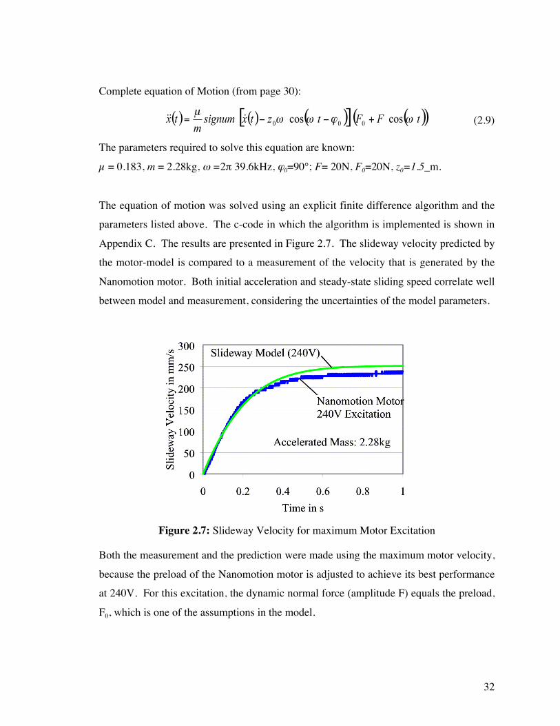
32

Complete equation of Motion (from page 30):


tx ωϕωωµ

coscos 000 +−−= &&& (2.9)

The parameters required to solve this equation are known:

µ = 0.183, m = 2.28kg, ω =2π 39.6kHz, ϕ0=90°; F= 20N, F0=20N, z0=1.5_m.

The equation of motion was solved using an explicit finite difference algorithm and the

parameters listed above. The c-code in which the algorithm is implemented is shown in

Appendix C. The results are presented in Figure 2.7. The slideway velocity predicted by

the motor-model is compared to a measurement of the velocity that is generated by the

Nanomotion motor. Both initial acceleration and steady-state sliding speed correlate well

between model and measurement, considering the uncertainties of the model parameters.

Figure 2.7: Slideway Velocity for maximum Motor Excitation

Both the measurement and the prediction were made using the maximum motor velocity,

because the preload of the Nanomotion motor is adjusted to achieve its best performance

at 240V. For this excitation, the dynamic normal force (amplitude F) equals the preload,

F0, which is one of the assumptions in the model.

33

To find out what effect the variation of phase and thrust force have on the slideway

motion as predicted by the model, the equation of motion is solved repeatedly for a

variety of values for ϕ0 and z0. Their effect is evaluated in respect of their effect on initial

acceleration and steady-state velocity, because initial acceleration and steady-state

velocity are the two major parameters that can be used to characterize motor

performance. A thrust force excitation of 400V is equivalent of a tip-vibration in the

slideway direction with an amplitude of z0=2.3µm. All other parameters were kept

constant:

Slideway mass = 1kg , excitation frequency = 41kHz, preload force = 10N, amplitude of

the dynamic normal force = 10N

The graphs in Figure 2.8 shows that solving the equation of motion for the motor-

slideway system for different amounts of thrust force excitation predicts that the steady

state slideway velocity is linearly proportional to the amplitude of the thrust force.

Figure 2.8: Theoretical Effect of Changes in the Thrust Force

It is assumed that the actuator excitation is linearly proportional to the amplitude of the

resulting vibration. The initial slideway acceleration does not seem to depend on the

thrust forces.

34

Figure 2.9 show the effect of variation of the phase between the dynamic normal force

and the sliding motion of the tip. The phase influences both initial acceleration and

steady-state slideway velocity. At a phase of zero the motor does not produce slideway

motion. The relationship between phase and slideway acceleration or steady-state

velocity is not linear, but continuous. Thus the both phase angle and the excitation of the

thrust force are suitable parameters to control slideway motion.

Figure 2.9: Theoretical Effect of Changes the Phase between the Thrust Force and the

Normal Force

What is not shown on the plot in Figure 2.9 is that for negative phase angles as well as

negative thrust forces the predicted acceleration acts in the opposite direction and the

steady state velocity has the same magnitude with the slideway moving in the opposite

direction.

2.4 Requirements for the New Motor Design

The proposed design of the new motor is based on the same driving processes as the

velocity mode of the Nanomotion motor (see page 9 in Chapter1). The main goal for the

35

design of an improved ultrasonic standing wave motor is that it performs as predicted by

the model for slideway motion: i.e. any excitation results in slideway motion and

slideway velocity. The key for such motor performance is the design of an actuator that

allows the independent excitation of dynamic normal force and thrust force. Both forces

are generated by actuator vibrations that have almost identical resonances but that are still

independent of one another. This design would make it possible to excite the dynamic

normal force with a constant amplitude. The problems associated with the transition

between static friction and sliding friction at slow slideway velocities are eliminated,

because once per cycle the normal load goes to zero, and any thrust force will initiate

sliding between motor tip and slideway.

If both actuator vibrations are independent, phase and/or thrust force determines the

slideway velocity. This offers three different ways to control the slideway motion:

1) The phase is constant at +90° or -90° and the thrust force determines the slideway

velocity. This is the most efficient mode of operation.

2) The thrust force is constant and the phase determines the slideway velocity. In order

for this strategy to perform well, the phase must not vary over time or slideway

position.

3) A combination of 1) and 2). If two control parameters are used, slower slideway

velocities are achieved with larger control parameters, which effectively lowers the

influence of electrical noise and nonlinearities in the amplifiers.

36

3 ACTUATOR DESIGN

The main objective of this project was to design a piezoelectric actuator that allows the

independent excitation of a dynamic normal force and a sliding motion, which is

proportional to the friction based thrust force. As the strain of the actuator material is

very small, the resonance effect is used to increase the amplitude of the vibration. Thus,

the actuator needs to have a resonance that predominantly generates the dynamic normal

force and another resonance that when excited only results in tip vibration in the slideway

direction. Then all parameters that determine the shape of the “sliding motion – normal

force” ellipse, shown in Figure 2.1, can be changed to control the slideway motion.

The major requirements for the dynamic behavior of the actuator are:

1 ) The two resonances of interest must be within 500Hz, so that one excitation

frequency excites both resonances.

2) Both resonances must (practically) not be coupled: the excitation of one vibration

must not excite the other and vice versa.

3) The prototype must be able to generate a dynamic normal force on the order of ±

20N.

4) The resonances must not change significantly over time.

5) Special attention must be paid to the boundary conditions of the actuator, for the

design as well as for the modeling of the prototype resonances. These conditions

include the location and method of motor support, as well as the influences of the

preload spring and the tip on both resonant frequency and the corresponding mode

shapes.

To develop a prototype which meets the specifications above, an actuator geometry has to

be identified which could generate the desired tip motion. Once a potential shape has

been found, dimensions which lead to the desired dynamic behavior must be determined.

Three different techniques have been used to in the actuator analysis and synthesis:

discrete methods using mass spring-models, distributed parameter models that use the

closed form solution of beam and rod elements and finite element analysis (FEA).

37

Discrete mass-spring models are a quick way to estimate the resonances of a system.

This methods require enormous simplifications in modeling the actuators and thus does

not predict the resonances precisely enough. Methods using distributed parameter

models yield better results, but models that accurately represent the actuator require

complex calculations that take a long time. FEA is the most useful tool to predict

actuator behavior, however this method is very time consuming because every iteration

requires the design of a new model.

Once the prototype is designed and built, measurements have to be performed to analyze

the actuators with the goal to iteratively improve modeling techniques. The concept of

modal analysis has to be mentioned, as both actuator synthesis and analysis is based on

resonance frequencies and mode shapes. The analysis of the systems resonances and

mode shapes cannot be used to predict the amplitude of the vibration, which determines

the slideway velocity and acceleration. The amplitudes of the actuator vibrations mostly

depend on how close the excitation is to the resonance and how much the air resistance

on the actuator surface and the damping losses in the glue layers affect the total damping

coefficient of the actuator. When a prototype is built, the actuator vibration needs to be

measured and then used in the slideway-motion-model (as presented in Chapter 2) to

predict the motor performance.

3.1 Vibration Analysis

For the dynamic analysis of undamped continuous or discrete systems the two most

important characteristics are natural frequency and mode shape [15]. They depend only

on the properties of the system, such as inertia and stiffness, and on boundary conditions,

including attached springs or masses. Mode shapes and natural frequencies do not

depend on excitation or initial conditions, thus offering a simplified method to

characterize a complex system.

38

Practically speaking, the natural frequency of an elastic body is characterized by a

relative maximum in the system’s response to a wide spectrum of excitation frequencies.

A mode shape represents the deformation of the resonating system at one point in time.

If an undamped system is excited with exactly one of its natural frequencies, the

amplitude of motion is theoretically infinite. However, in the presence of damping, the

system will deflect in a shape proportional to the mode shape and oscillate with the

excitation frequency (the natural frequency for that mode).

Mathematically, a natural frequency or eigenvalue represents a nontrivial solution to the

differential equation of the system. Mode shapes are the eigenvectors for the

corresponding eigenvalues (natural frequencies). Each eigenvalue substituted back into

the general solution represents one possible solution to the homogeneous differential

equation of the system. Mode shapes cannot yield any information on amplitude or phase

at any given coordinate since they do not depend on initial conditions, time or forcing

functions. For this reason they are commonly normalized.

Figure 3.1: Modal Participation

39

Only the complete solution to the equation of motion describes the actual motion of the

system. This solution can be obtained by linear superposition of all possible mode shapes

in combination with modal participation factors. Figure 3.1 sketches the composition of

a frequency spectrum for a system with three resonances or three degrees of freedom.

Note that Figure 3.1 is not drawn to scale as the spacing between the resonances is much

larger than what is represented and the relative amplitudes decrease more rapidly with the

order of the resonance than what is drawn.

The modal participation factors determine how much each mode influences the actual

vibration of the system. The modal participation depends on initial conditions for

homogeneous problems or forcing functions for transient problems. Generally, the closer

the natural frequency of a mode is to the excitation frequency and the closer the static

deflection of the excitation force is to the shape of the mode, the larger the participation

factor of that mode. For example, if the system in Figure 3.1 is excited near its first

fundamental frequency, the system response consists of approximately 96% of mode 1,

approximately 3% of mode 2 and 1% of mode 3. When excited between modes, at

frequency ω*, this ratio changes and the resulting vibration consists of 55% of mode 2,

40% of mode3 and to 5% of mode1.

Although modal participation factors can be calculated, for most real systems this is a

difficult process and the quality of the results largely depends on hard to control factors

such as the damping ratio and the excitation force. For the development of the motor, it

seems more feasible to design an actuator that has two mode shapes, each of which

resembles one of the desired actuator vibrations. Their frequency must be close together,

but excitation and geometry need to be chosen in such a way that the modal participation

factors are very selective. For example, the participation factor for excitation 1 and the

first mode is very large but small (ideally zero) for the second mode. Excitation 2,

although at the same frequency as excitation 1, results in little or no participation of the

first mode but almost 100% participation of the second mode. How well this goal can be

achieved directly determines the quality of the motor.

40

3.1.1 Analytical Methods

Three different techniques have been used in analysis and synthesis of the actuator:

discrete methods using mass-spring models, distributed parameter models that use the

closed form solution of beam and rod elements and finite element analysis (FEA). Figure

3.2 shows how a model of a piezoelectric actuator can be created.

Discrete models reduce the real system to spring, mass and damper elements. The

masses are modeled as if they are concentrated at one point and the spring elements must

be chosen such that they represent the elasticity in the real system. Whereas the real

actuator can vibrate in every direction with an infinite number of resonances, the discrete

mass-spring model in Figure 3.2 reduces the problem to two degrees of freedom in one

direction. The same simplifications that make mass-spring models so easy to solve cause

limitations in their use: The number of masses used in the model determines the highest

order of resonance that can be predicted. Also, determining the equivalent masses in the

models is in part based on assumptions of how the actuator vibrates. The quality of the

result of the mass-spring model largely depends on how accurately the real system is

represented by the model. However, mass-spring models offer a quick method to define

relationships between certain parameters such as length or width of the actuator and the

natural frequencies of the system.

Methods using distributed parameter models yield better overall results. In the example

shown in Figure 3.2, very few modeling assumptions have to be made. The vibration of

the piezoelectric ceramic can be described using the closed form solution of a beam or

rod element. An infinite number of resonant modes can be predicted. This solution,

which is based on the complete equation of motion of the entire length of the element, is

available in general form for simple geometries (strings, rods, beams etc.) [15] [16].

Applying the appropriate boundary conditions (preload spring and tip-stiffness) to the

general beam vibration solution is the only modeling that has to be done in the distributed

parameter model. To model more complex geometries, multiple beam elements can be

connected via the corresponding boundary conditions. This makes it easy to model

41

systems that consist of different materials or include non-trivial shapes. The main

disadvantages of using distributed parameter systems are a) that computation time

increases exponentially with the number of elements in the model and b) that the solution

process becomes very complicated if non-isotropic materials have to be modeled.

Piezoelectric materials, for example, are highly anisotropic.

Figure 3.2: Mass-Spring Model (a) and Continuos Beam in Bending (b) of a Rectangular

Actuator

3.1.2 Numerical Analysis

Repeated analysis of different prototypes showed that it is essential to consider the

anisotropic material properties of the piezoelectric ceramic, the exact dimensions of the

prototype and the different material of all components, especially all glue joints. The thin

layers of epoxy glue between all components influence the natural frequency of the

structure.

Rather than using very complex models with distributed parameter elements, an iterative

process based on several FEA models was designed to numerically determine all natural

42

frequencies and mode shapes of a system. The results were then analyzed and the

dimensions of the system were modified. This process was repeated until a system was

obtained for which the two desired longitudinal modes were at similar frequencies.

3.1.2.1 ANSYS

ANSYS (an FEA program) is a powerful tool to perform modal analysis. It allows the

operator to design accurate models of the prototype that consider anisotropic materials, to

include the influence of the piezoelectric effect on the material stiffness, the exact

geometry as well as complex boundary conditions. Resonances for modes in all three

dimensions can be predicted.

The major sources of error using FEA based modal analysis are caused by the limited

number of elements used in the model and by simplifications in the boundary conditions.

The use of thin elements leads to errors. Modeling thin features in the prototype such as

flexure elements or glue joints that are only 50µm thick, leads to numerical problems

within the glue elements. The number of elements needed to obtain an acceptable aspect

ratio of the glue elements by far exceeds the available memory to store elements and

results.

3.1.2.2 Boundary Conditions

The main boundary conditions in the actuator model are given by the tip-slideway

contact, the preload spring and the motor support. The motor support is only considered

in the final model, because it must not influence resonances and mode shapes of the

actuator. Constraining any part of the model that is not a node will influence the result.

Once the analysis is completed, the motor support can be included. If the location of the

support is chosen correctly, neither the predicted mode shapes nor any resonance will

change.

43

The preload spring is too soft for its stiffness to have a significant influence on the result.

Its mass, specifically its rotational inertia, does make a difference and needs to be

considered. The tip-slideway contact has been modeled as a linear spring element. Its

stiffness was determined using the equations for Hertzian deflection, given that the

contact area is determined solely by the static preload. The contact stiffness theoretically

increases for increasing contact forces and vice versa, but this effect cannot be considered

as modal analysis does not yield information about vibration amplitudes. Measurements

proved that this simplification does not affect the predictions.

Thus, using discrete parameter models, the actuator model can be reduced to a few beam

elements, and a solution can be obtained quickly that directly yields information on the

influence of individual parameters on the resonances and mode shapes. This solution is

not precise enough to be used alone as a method to construct a prototype; however, this

method can be used as a base to start finite elements analysis to fine-tune the actuator.

This greatly reduces the number of FEA model iterations.

3.2 Vibration Measurements

The first prototypes that were built based on the vibration analysis as described above did

not generate slideway motion the way it had been expected. This demonstrates the

importance of measuring and calculating both the resonance frequency and the mode

shapes, which iteratively improves the actuator design. In addition measurements of the

amplitudes of the actuator vibrations, which cannot be predicted by modal analysis, allow

comparison of the observed motor performance to the one predicted by the model for

slideway motion in Chapter 2.

Whereas resonances are relatively easy to measure, mode shapes measurements are more

difficult to perform. In real, vibrating systems generally more than one mode shape is

present. Calculated mode shapes usually describe the motion of the center plane of the

vibrating object.

44

In the experimental vibration analysis, actuator motion can only be measured on the

surface. Although analysis might be a two-dimensional problem, one needs to be aware

that the object that is being measured experiences strain in all three directions. For

example, the longitudinal vibration of an actuator as in Figure 3.3 on the left also causes

the thickness of the actuator to change. If the vibration amplitude is only measured at a

single location, this measurement cannot be clearly distinguished from the measurement

of a bending vibration of the same actuator as sketched in Figure 3.3 on the right. Only

when the vibration amplitude is measured at multiple locations along the actuator surface,

as shown in Figure 3.3 on the bottom, can the phase between excitation and every

individual measurement be used to distinguish between longitudinal and bending motion.

Figure 3.3: Mode Shape Measurements

45

3.2.1 Piezoelectric Force Sensor

To evaluate the ability of a prototype to move a slideway, the most desirable

measurement would be to directly measure the forces at the tip because only the forces or

motion at the tip cause slideway motion. As long as the stiffness of the force sensor is

similar to the stiffness of the slideway, the measurement does not influence the tip

vibration. One way to measure forces at the tip is to use a piezoelectric force sensor.

Piezoelectric force sensors use the piezoelectric effect in which an external force causes

strain which results in a charge imbalance in the material that can be detected. A

piezoelectric force sensor by Kistler (type 9251A) is available for those measurements.

Its bandwidth is limited by the resonance of the mass that is attached to the sensor and the

stiffness of the sensor itself (sensor stiffness =300N/µm). For the sensor to resonate at a

frequency of 40kHz, a mass of 4.7g needs to be attached to it. Furthermore, the

sensitivity of the sensor changes when the measured frequency is close to the sensor

resonance. In this case, the sensor still gives limited information about the resonance

frequency, but the measured amplitude exceeds the true amplitude.

3.2.2 Optical Displacement Sensor

Another way to measure actuator vibration is to use an optical displacement sensor. This

device is characterized by a high bandwidth (above 100kHz) and a range of about 0.5mm

with nanometer resolution, which is more than sufficient. As this sensor does not need to

touch the vibrating actuator, it is ideal because it cannot affect the vibration by measuring

it.

This sensor uses light, emitted though an optical fiber onto the vibrating surface. The

reflected light is collected with additional optical fibers that are arranged around the

emitting fiber. The amount of light reflected off the diffuse surface, as shown in the

calibration curve of the device in Figure 3.4, depends on the distance between the sensor

and the target. The calibration curve in Figure 3.1 also reveals that there are two regions

46

where the sensor output is linearly proportional to the distance from the target, labeled

“Front Slope” with a range between 0.3mm and 0.7mm, and “Back Slope” with a range

between 1.1 and 1.7mm. The gradient of the respective slope is the sensitivity of the

instrument.

Figure 3.4: Optical Displacement Sensor

Among other things, the sensitivity depends on the optical properties of the surface.

Damage to the actuator surface, such as scratches, impair the quality of the

measurements. Because the instrument needs to be calibrated for every surface,

reflective Mylar tape is attached to the actuator. A detailed description of the calibration

and setup procedure can be found in Appendix D.

3.3 Prototypes

3.3.1 L-shaped Prototype

The goal of this project was to design an actuator that allows the excitation of a 2-

dimensional vibration as described in Chapter 2.3. The first potential solution was to

47

arrange two piezoelectric actuators at a 90° angle and to use the longitudinal vibration of

each actuator to generate one component of the desired vibration.

The design principle which was implemented in the first prototype, is sketched in Figure

3.5. Two orthogonal beams of solid piezoelectric ceramic were glued at right angles to a

metal block, to which a wear resistant alumina tip was attached. Actuator 1 provides

excitation in the direction of slideway motion, and Actuator 2 changes the normal load at

the contact point between the ceramic tip on the motor and the slideway drive surface.

The spring is used to preload actuator 2, which mainly provides the friction force

between motor and slideway. Keeping the brittle piezoelectric ceramic compressed

would be beneficial to avoid fractures but the load required to completely balance the

tensile stress is greater than the buckling load of the structure.

Figure 3.5: L-Shaped Prototype

48

The control strategy for this design is to excite both actuators with the same frequency

and to change the phase between the excitation of Actuator 1 and Actuator 2 to reverse

the direction of slideway motion. The two masses at the ends were instrumental in

adjusting the position of the vibration nodes (points of zero amplitude). The location of

these nodes is an important aspect of the design because this is where the motor is

attached to the frame to support the drive loads.

Experiments showed that, when Actuator 2 was excited with +/- 100V at 44.8kHz, the

motor produced considerable slideway motion (in only one direction) and a pushing force

of approximately 5N. The excitation of actuator 1, however, does not influence the

motor’s performance notably. A change in phase between both excitations changes the

magnitude of the pushing force and slideway velocity to some extent, but does not allow

a reversal of the direction of motion.

This observation led to the conclusion that mode shapes of the actuator vibrations must

be measured in order to understand the actuator vibration that leads to the observed

behavior. The optical displacement sensor is used as described in Chapter 3.2.2, and the

measurement is triggered by the excitation voltage, which allows measurement of the

phase at each location. This shows whether the measured location moves closer to the

sensor or away from it at the reference time. The measurements were repeated for

multiple points along the actuator surface. The results are shown in Figure 3.6. The

measured mode shapes are projected above the contour of the prototype. The excitation

of actuator 2 at 44.8kHz (Figure 3.6 on the left) causes the tip to vibrate in the vertical

direction, which primarily excites a longitudinal resonance (this cannot be displayed

together with the mode shape). The mode shape measurement at 44.8kHz revealed a

significant component of bending excitation in actuator 2 at that frequency, which was

not predicted in the actuator analysis.

49

Figure 3.6: Mode Shape Measurement of the L-shaped Prototype

The measurement in Figure 3.6 on the right shows that excitation of Actuator 1 generates

horizontal tip motion in addition to a bending moment, which then causes a bending

vibration in Actuator 2. Although excitation of Actuator 1 causes the prototype to vibrate

at the predicted mode shape, the horizontal tip motion caused by the bending motion of

Actuator 2 when Actuator 2 is excited, is larger than the tip motion caused by the

longitudinal excitation of Actuator 1. Consequently the excitation of Actuator 2 alone

generates the excitation “force-motion ellipse” at the tip, which is responsible for the

observed slideway motion.

50

3.3.2 T-shaped Prototype

A prototype with a T-shaped geometry was introduced to add symmetry to the L-shaped

design with respect to the bending motion of Actuator 1 when Actuator 2 is excited. The

goal of this design is to be able to excite Actuator 2 without causing any tip motion in the

direction of slideway travel. Figure 3.7 shows a sketch of the T-shaped prototype. For

any symmetric design, the bending moments within Actuators 1 and 3 caused by the

longitudinal vibration of Actuator 2 are equal in magnitude but opposite in phase and thus

effectively cancel each other at the tip. It is not possible to implement the same

improvement for the longitudinal excitation of Actuators 1 and 3. When Actuators 1 and

3 are excited to generate sliding motion, bending vibration occurs in Actuator 2. The

dimensions of the motor can be chosen such that rotation of the tip is small; however it

cannot be eliminated entirely by symmetry as was done for the other direction.

Consequently, longitudinal excitation of Actuators 1 and 3 results in bending motion of

Actuator 2, which in turn leads to bending in Actuators 1 and 3. Since bending of these is

a component of the mode shape that generates the normal force at the tip, the longitudinal

excitation of Actuators 1 and 3 also results in a dynamic normal force at the tip.

Although both modes are still slightly coupled, the advantage of this prototype is that the

effect of one mode on the other is much smaller than in the L-shaped prototype.

Figure 3.7: T-shaped Prototype

51

The masses at the free ends of the actuators are a very effective tool to adjust the

resonance frequencies and node positions. An increase in mass generally lowers the

resonance frequency of the longitudinal resonance of the respective actuator and the

nodes moves closer toward the mass. The prototype is supported via four rubber cylinder

which are located at the common longitudinal and bending nodes at Actuators 1 and 3.

Rubber was chosen, because it is soft and light and thus very unlikely to influence the

dynamic behavior of the motor to the extent to which it was observed in the L-shaped

prototype. For future motor operation, a stronger support is requires to maintain the

motor alignment, but the current configuration permits easier analysis of the actuator.

3.3.2.1 Experimental Results

Experiments showed that a dynamic normal force of +/- 30N was generated for an

excitation voltage of +/-100V at Actuator 2. Unlike Prototype 1, it could be confirmed

that the excitation of Actuator 2 in Prototype 2 generates predominantly a dynamic

normal force at the tip while the thrust force is very small. A maximum slideway

velocity was measured at about 0.5m/s, when both actuators were simultaneously excited

and the phase was set to the optimal value.

The basic experimental setup and a measurement of the tip forces as a function of the

excitation frequency are shown in Figure 3.8. The motor is preloaded against a

aluminum oxide plate which is mounted onto the piezoelectric force sensor, which

measures forces in the horizontal direction (slideway motion) and vertical direction. The

presented measurement represents several similar measurements. The excitation

frequency was swept through a much larger range than shown in Figure 3.8, however

only the motor’s response at frequencies around the two resonances of interest is relevant.

52

Figure 3.8: Force Measurement, ±100V Excitation

The resonance of the force measurement setup limits the bandwidth of the force sensor.

This resonance is composed of the sensor stiffness and the mass of the sensor, the preload

bolt and the aluminum oxide plate. It is difficult to exactly predict its resonance

frequency, but assuming a mass of 3g mounted onto the sensor leads to a sensor

resonance at 50kHz. As the components of the experimental setup add up to a very

similar mass, the measured frequency is close to the sensor resonance and thus the

sensitivity of the force sensor changes within the measured frequency spectrum. The

frequency of the resonance peaks in Figure 3.8 should be unaffected.

One problem with the operation of this motor is that there is no clear mechanism by

which the resonances can be adjusted relative to each other. As the graph of the force

measurement in Figure 3.8 shows, the natural frequency of the mode that generates the

thrust force is about 2.5kHz above the resonance that generates the normal force. This

difference should be reduced to approximately 500 Hz for the motor to utilize the full

potential of the resonance effect. No matter how well the analysis is done to develop the

motor, it is virtually impossible to build the prototype such that both resonances are at

53

exactly the same frequency. Therefore it must be possible to modify the length or width

of one actuator or the attached mass to fine-tune the motor, in the model and after a

prototype has been built. This does not seem feasible with either the L-shaped or the T-

shaped design, because all alterations of the L-shaped and T-shapes prototypes influenced

both mode shapes and resonant frequencies to about the same extent. If, for example, the

length of one actuator is reduced, each individual resonance increases, but the difference

between both resonances does not change significantly. Based on the force spectrum

shown in Figure 3.8, it is amazing that the T-shaped prototype is capable of generating

slideway motion of 500mm/s.

3.3.2.2 Thermal Effects

Slideway motion was generated with the t-shaped prototype even though the resonances

of the actuator were about 2.5kHz apart,. However after about 5 minutes of operation, it

was observed that the motor performance decreased. Repeated measurements of the

frequency spectrum showed that the resonance had changed. Eventually the prototype

came apart at the glue joints.

Figure 3.9: Temperature Measurement

54

Constant excitation at the operating resonance caused the actuator to get very hot. Figure

3.9 shows one of many temperature measurements on the steel mass at the bottom of

Actuator 2 and at the connection between the actuators (aluminum). In the experiment

shown in Figure 3.9 the temperature at the end of Actuator 2 increased to well above

160°C after less just 22 seconds of motor excitation. The steel mass was replaced with a

ceramic mass to see if the magnetic permeability or the electrical conductivity of the

material was the source of the problem. The altered actuator seemed to stay cool at first,

but further experiments showed that this was misleading. Using the steel mass, heat that

is generated in the actuator is quickly conducted through the steel and can be measured at

the surface. A ceramic mass does not conduct heat as well, so even if heat is generated in

the middle of the actuator, it cannot be as easily detected at the surface.

The heat in the prototype is a result of the elastic damping of the glue caused by strain

energy in the vibrating system. A model of the prototype was developed by calculating

the strain energy in a simple beam that vibrates similarly to Actuator 2 in Figure 3.9 on

the left. The amplitude of the vibration was set to 10µm, which is the upper limit of the

vibration that can be expected in the prototype. All components were initially assumed to

have the (low) damping loss of the piezo-ceramic material. Under these conditions, the

temperature within the actuator reached a steady state value of about 60°C. Such a

temperature would barely be acceptable for stable operation of the motor.

The loss factor η, also called ( )δtan , is a material constant that relates the total vibration

energy in the system, W, to the energy dissipated per cycle, ∆W.

ηπ2=∆

W

W (3.1)

Thus, with a loss factor of η = ⋅ −1 111 10 3. as specified by the manufacturer, 0.7% of the

vibration energy is lost during each cycle. Information about the loss factors of the epoxy

that was used to build the prototypes could not be obtained; however, epoxy-materials

typically used in fiber reinforced composites [16] are between η= 22 10 3⋅ − and

55

η= 43 10 3⋅ − which is equivalent to an energy loss of 14% and 27% (of the systems

energy per cycle) respectively.

Since the epoxy-glue has a considerably higher damping loss and experiences higher

strain than the rest of the actuator (for the same stress), it can be assumed that although

the volume of the epoxy is fairly small, most of the heat is generated within the glue

joints. The poor heat conductivity of the piezoelectric material, which is approximately

1.2W/(kgK), makes it even more difficult to detect a temperature increase in the center of

the actuator and also keeps the heat in the glue joint where it causes most damage. When

the glue reaches its temperature limit, the polymers within the glue disintegrate and the

glue loses its strength.

To lower the amount of kinetic energy that is transformed into heat, the same actuator

could be made from a single piece of piezoelectric material, thus eliminating the glue

joints between the actuators. Because this change in design neither solves the problem of

coupling between both modes nor shows a strategy to individually adjust one resonance

relative to the other, a different prototype had to be developed.

3.3.3 I-shaped Prototypes

The main motivation for the development of the I-shaped prototype, which is illustrated

in Figure 3.10, was to eliminate the glue joints found in the first two prototypes as well as

the problem of the coupling between different mode shapes. The basic idea was to use a

longitudinal and a bending resonance in a beam shaped actuator. Both resonances are

geometrically independent (uncoupled) and the bending resonance does not excite the

longitudinal resonance as long as the design is symmetric in all directions.

The electric field is applied between one of the electrodes on the outer surface (1) or (2)

(in Figure 3.10) and the brass electrode in the center. Applying a sinusoidal voltage at

the outer electrodes (1) extends and contracts the upper half of the actuator and thus

excites the bending mode. An electric field that extends across the actuator will excite

56

the longitudinal mode of vibration. This is done by applying voltage to the inner

electrodes (2). Because these two modes are orthogonal, it is virtually impossible to have

any interaction between them.

Figure 3.10: I-shaped Prototype

This design does not have highly stressed glue joints. The main glue joint is loaded in

shear, not in tension and compression as was the case in the previous designs. Because

these resonances are determined by fewer factors than those of the T-shaped prototype,

the dynamic analysis of the I-shape is relatively straight forward. Analytical solutions for

simple beam vibrations can be used to approximate the desired dynamic behavior

followed by FEA models to obtain more precise results.

The masses at the end of the actuator are the primary tool to individually change the

longitudinal resonance and node positions independently of the bending vibration. If the

inertia is located at a point that experiences large amplitudes of motion, it lowers the

natural frequency of the respective mode and moves the node towards it. The

57

longitudinal mode shape has an anti-node at the end, the bending mode shape has a node

close to the end. This means that the inertia of the mass has a bigger effect on the

longitudinal vibration than on the bending resonance.

3.3.3.1 Actuator Excitation and Resonances

The I-shaped prototype uses the fifth bending mode to generate a dynamic normal force

and the second longitudinal mode to generate sliding motion in a very similar manner to

the T-shaped prototype. The results of the finite element model that was used to design

the prototype is shown in Figure 3.11. The actuator vibration was measured at two

locations. The measurement at the end of the actuator yields information about the

longitudinal resonance. The large peak slightly above 35kHz is the first longitudinal

resonance, the smaller peak at 64kHz is caused by the second longitudinal resonance.

The second measurement was performed to determine the bending resonance of the

actuator. Both the frequencies of the bending resonance and the longitudinal resonance

correspond well with the prediction. From the results shown in Figure 3.11, it is

impossible to gain information about the mode shapes. However, the measured

resonances are within 1kHz of the predicted resonant frequencies.

The decision to use the second longitudinal mode means that the motor can be supported

at the two nodes of the second longitudinal mode shape. This also means that the motor

needs to have a bending mode that has nodes at these two locations. To use the first

bending mode would be ideal, but its natural frequency is much too low. The third

bending mode (as well as all modes with even numbers) could not be used because the

node locations could not be made to match the nodes of the longitudinal mode. However,

using the fifth bending mode, dimensions could be found such that both resonant

frequencies and node locations match. The best tip location is in the middle of the

actuator, as shown in Figure 3.10 and Figure 3.11, because that is the location on an anti-

node of both mode shapes and the bending mode does not have a component in the

longitudinal direction of the actuator. Thus the bending vibration will only generate a

dynamic normal force but no sliding motion or thrust force.

58

Figure 3.11: Mode-Shapes with Corresponding Resonant Frequencies

3.3.3.2 Motor Performance

Initial measurements of the frequency spectrum for the forces at the tip indicated that the

resonances for the normal force and for the thrust force differed by about 2 kHz. This

difference was carefully reduced by adjusting the masses at the ends of the motor.

Despite matching resonances, this prototype was not capable of generating slideway

motion. Even after both resonances had been adjusted to be close to the driving

frequency of 63.1kHz, the dynamic normal force of +/-4N was too small to overcome the

static frictional forces induced by the preload. Although the I-shaped Prototype has not

been tested with the highest possible electrical field (+/-800V at the electrodes),

extrapolation based on measurements at lower excitation voltages suggests that the

59

required dynamic normal force of +/- 20N cannot be achieved, even if power amplifiers

capable of supplying the maximal voltage at 63kHz were available.

A new prototype had to be developed, that is more efficient in generating a dynamic

normal force but that still exhibits the major advantages of the I-shaped prototype.

3.3.4 I+ Prototype

The basic ideas of the design concept of the I+ prototype are 1) to use the modes of the

lowest possible order and 2) to use a longitudinal mode to generate the dynamic normal

force. In general, the lower the order of a vibration, the larger the amplitude for the same

kinetic energy. Because the best location for the motor support is at the common nodes

of both resonances, using the first longitudinal resonance of a beam-shaped actuator

means that the motor can only be supported at one node (which is in the middle of the

actuator). Consequently, the bending mode that generates the thrust force at the tip must

have a node in the center of the actuator as well.

3.3.4.1 Actuator Design

A sketch of the I+ design is shown in Figure 3.12. The two pieces of piezoelectric

material are polarized in opposite directions. Exciting electrodes 2 and 5 with a

sinusoidal excitation voltage excites only the longitudinal vibration mode. This allows

the adjustment of the dynamic normal force at the tip such that the normal force

alternates between almost no compression and twice the preload. The bending vibration

is effectively excited with a sinusoidal voltage at electrodes 1 and 4 and with the inverse

of this voltage at electrodes 3 and 6. This concept is very similar to the I-shaped design.

Note that when both vibrations are excited, the entire volume of the actuator is being

used.

60

Figure 3.12: I+ Prototype

This prototype is dimensioned such that the first longitudinal and the second bending

resonance (s-shaped) can be excited at 41.5kHz. If the design is symmetrical with respect

to its center, both mode shapes have a common node at the center. This simplifies the

design process, because only the resonant frequencies, but not the node locations, have to

be considered during the design process.

3.3.4.2 Actuator Construction

An improvement over the previous prototype lies in the composition of the actuator.

With the I-shaped prototype, the electrodes on the sides of the piezoelectric plate facing

the center electrode were removed when the thickness of the piezos was reduced from 3

to 2 mm. Figure 3.13 shows the composition of the actuator. It consists of two

piezoelectric plates that are glued together with a brass electrode in between the plates.

Holes in the brass electrode allow the glue to directly bond the piezoelectric plates to one

another, which minimizes the thickness of the glue layer.

61

Figure 3.13: Composition of the I+ Actuator

The electric field has to go from the outer electrode through the piezoelectric material,

then through the epoxy layer to the center electrode (which is the electrical ground for all

signals). For the I+ design, the silver electrodes were left on both surfaces of the

piezoelectric plate when they were glued to the center electrode. The idea is that the glue

acts from the silver electrode on the surface of the piezoelectric plate through the holes of

the center electrode to the surface of the other piezoelectric plate. The surface roughness

of the center electrode, especially around the holes, in combination with a very thin

epoxy layer will allow the center electrode and the silver electrode on the surface of the

piezoelectric material to touch. This will prevent the electric field from diminishing over

the width of the epoxy layer. A stronger field is left to excite the piezoelectric material.

The use of epoxy, which has silver particles to make it electrically conductive, led to a

small but detectable increase in vibration amplitude. However, not enough prototypes

were tested to confirm whether this difference could be attributed primarily to the

62

conductivity of the epoxy or to small differences in the actuator dimensions leading to

better excitation of both resonances.

3.3.4.3 Actuator Excitation and Resonances

Measurements showed that the first version of the I+ Prototype was capable of generating

the required dynamic normal force of +/-20N and the longitudinal resonance within

200Hz of the predicted frequency. However, the bending resonance was about 4 kHz

higher than expected. After the original FEA model had been checked for errors and the

dimensions of the prototype were compared to the model, no deviations could be found.

To solely investigate the dynamics of the actuator without any influences from the

preload and the tip-slideway contact, experiments were performed where the actuator was

not preloaded and thus not in contact with the slideway. The model was altered

accordingly. The measured resonant frequencies, mode shapes and amplitudes were in

agreement with all predictions. Thus, the problem that the bending resonance is 4kHz

higher than predicted, has to be due to incorrect modeling of the boundary conditions

(motor support, preload spring, tip-slideway contact).

Since the influence of the frictional forces under sliding conditions on the resonance must

be much smaller than the effect of the stiffness and the inertia of the actuator, the tip (in

the FEA model) was not constrained in any way in the sliding direction. The assumption

that the frictional force is negligible is valid when the motor is running and both actuator

vibrations are at resonance. When only the resonance in the sliding direction is excited,

the motor does not produce slideway motion and the tip never slides along the slideway

surface. In this case the resonance is higher because the tip experiences an elastic

resistance. In other words, to compare the measured resonances to the predicted

resonance, the stiffness of the tip-slideway contact must be included in the FEA model to

correctly predict both actuator resonances when excited individually. Whether or not the

tip slides along the slideway surface thus has a significant influence on the boundary

conditions needed to design an appropriate model. To determine these conditions, spring

elements were added to the FEA model of the I+ prototype. The corresponding tip

63

stiffness in the slideway direction was determined using an FEA model of the tip. A

force of 10N was applied tangentially on the tip and compared to the displacements it

generated. With this stiffness the FEA model of the I+ prototype exactly predicted the

measured resonance. Note that the additional springs in the slideway direction in the

model are added solely for the purpose of explaining the measured resonances when

excited individually. Prototypes of both designs are able to produce slideway motion.

The final prototype is based on the model that includes the tip stiffness in the direction of

slideway motion, mainly because it is possible to individually measure each resonance

and thus evaluate the modeling success.

The operational frequency varies from one motor to another. The manufacturing process

resulted in slightly different actuator dimensions for each individual prototype, which

caused the resonances to vary between 40.0 and 41.5 kHz for the five prototypes of the I+

design that were built. It should be mentioned that small deviations from the modeled

actuator dimensions influence both resonances to a similar extent, which means that for

all tested I+ type prototypes, both resonances were close enough to maintain an almost

identical motor performance.

3.3.4.4 Motor Support

For all prototypes to this point, a soft support consisting of two rubber cylinders was used

because the softer it is the less potential it has to affect the dynamic properties of the

motor. A soft support does reduce the bandwidth of the motor-slideway system because

it introduces the possibility for the slideway mass and the motor support stiffness to

resonate.

In addition, a soft motor support allows the driving forces to rotate the motor. If the

motor loses its alignment with the slideway (90º to the slideway surface), a certain

component of the longitudinal vibration that is supposed to generate only a dynamic

normal force also acts in the sliding direction. This process is illustrated in Figure 3.14

a). In terms of controlling the slideway position, the motor rotation means that the phase

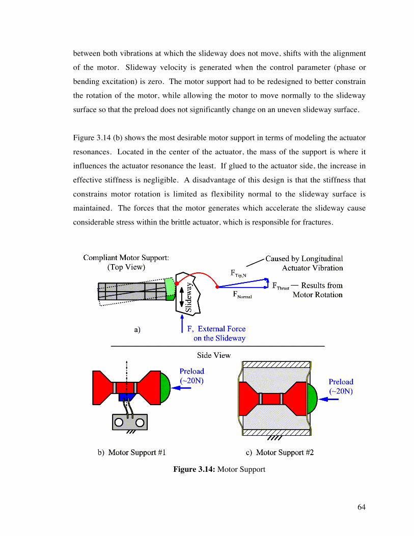
64

between both vibrations at which the slideway does not move, shifts with the alignment

of the motor. Slideway velocity is generated when the control parameter (phase or

bending excitation) is zero. The motor support had to be redesigned to better constrain

the rotation of the motor, while allowing the motor to move normally to the slideway

surface so that the preload does not significantly change on an uneven slideway surface.

Figure 3.14 (b) shows the most desirable motor support in terms of modeling the actuator

resonances. Located in the center of the actuator, the mass of the support is where it

influences the actuator resonance the least. If glued to the actuator side, the increase in

effective stiffness is negligible. A disadvantage of this design is that the stiffness that

constrains motor rotation is limited as flexibility normal to the slideway surface is

maintained. The forces that the motor generates which accelerate the slideway cause

considerable stress within the brittle actuator, which is responsible for fractures.

Figure 3.14: Motor Support

65

The motor support as shown in Figure 3.14 (c) offers the highest possible resistance to

rotation of the motor. The motor forces are not transmitted through the actuator, which

has prevented actuator fractures to date. The flexures in this support are not located at

nodes of the actuator as they were added to the design after the actuator itself was built,

This impedes both bending vibration and the longitudinal vibration. The maximal motor

velocity is reduced from 500mm/s using the flexure as shown in Figure 3.14 b) to

300mm/s using the flexure elements on both ends of the actuator (c). On the other hand,

the motor preload can be increased significantly without breaking the motor, which leads

to an increased slideway acceleration.

3.3.4.5 Open Loop Motor Performance

Figure 3.15 shows series of measurements of the slideway velocity when a constant

bending excitation is applied to an initially motionless slideway. Motor support #2, as

defined in Figure 3.14, is used to hold the actuator in place. In this experiment, an air

bearing spindle is used as the slideway. Its inertia is equivalent to a linear slideway with

a mass of 2.28 kg. When the excitation voltage is applied, the slideway accelerates until

a steady state velocity is reached. The slideway velocity is very constant for both high

and low levels of excitation. Changing the phase leads to very similar motor

performance except that the same bending excitation results in slower slideway motion.

The latter decreases to a standstill for a phase of 0º or 180º. It should be noted that the

initial acceleration is virtually independent of the excitation amplitude. Instead, it

depends on the preload, the accelerated mass, the coefficient of friction, and the phase.

The steady state slideway velocity is linearly proportional to the bending excitation. This

becomes apparent when the steady-state slideway velocity from the measurement in

Figure 3.15 on the left is plotted as a function of the excitation voltage as done in Figure

3.16.

66

Figure 3.15: Slideway Velocity for Different Excitation Voltages

Figure 3.16: Steady-State Slideway Velocity

The measurement of the steady-state slideway velocity in Figure 3.16 shows that, unlike

most conventional standing wave motors, any excitation of the bending amplitude or

thrust force results in slideway motion. The smallest obtainable constant slideway

67

velocity is essentially limited by the noise and the linearity of the electric components

that generate and amplify the sinusoidal excitation voltage. For negative excitation

voltages the slideway velocity has virtually the same magnitude but the direction of

motion is reversed.

68

4 CLOSED LOOP POSITION CONTROL

The new ultrasonic piezoelectric motor whose development was described in Chapter 3

was designed as an actuator for applications that require fast response time, high

resolution and power off holding abilities. Open loop testing has shown that the motor

generates slideway motion such that the steady state velocity is proportional to the

bending excitation. To fully characterize the motor and to demonstrate its full potential

for positioning tasks, the motor has to be tested in a closed loop control system. This

chapter will describe the process of finding a simple control strategy that leads to

satisfactory motor performance.

The system’s response to a step input is seen as the most important characteristic. The

system is evaluated in respect to stability, steady-state accuracy, response time and the

possibility to avoid overshoot using simple proportional gain and PID-control algorithms.

It is the goal of this research to characterize the motor and to show its basic performance,

including typical sources of error, but not to develop a specific control algorithm.

Figure 4.1: Photograph of the Motor-Slideway System

69

4.1 System Setup

Figure 4.2 shows a block diagram of the closed loop control system. The Computer-

Motor interface transforms the control parameter into the signals that are required to

drive the motor. The two voltages that oscillate at the motor frequency of 40kHz are

modulated such that the control parameter is proportional to either the phase angle

between both motor vibrations or to the amplitude of the signal that excites the thrust

force. Power amplifiers are used to achieve a maximum output voltage of +/- 500V at the

actuator. The slideway position, the goal of the control effort, is measured using an

incremental encoder with a resolution of 11.08µm and compared to the commanded

position. The error is the difference between commanded and measured slideway

position, which is the basis for the control algorithm to compute the appropriate motor

control value.

Figure 4.2: Block Diagram of the Closed Loop System

It seems practical to use a single transfer function that represents the behavior of the

computer-motor interface, the power amplifiers (Trek 50/750) and the motor-slideway

system. This transfer function GM(s) describes the slideway position as a function of the

70

control parameter. The use of a different control parameter required a different transfer

function.

The controller is implemented using a computer, which allows almost unlimited

flexibility of the controller algorithms. The sampling rate is the frequency at which the

slideway position is measured and made available for the controller and at which the

updated amplitude and/or phase values are sent to the motor. The sampling rate needs to

be slower than the motor operating frequency, and at least 10 times higher than the

bandwidth of the system. It is also limited by the ability of the computer to perform all

necessary calculations and the speed of the interface to collect and emit the data. A

sampling rate of 500Hz is sufficient considering the large inertia of the slideway, which

is equivalent of 2.28kg in linear motion.

4.1.1 Computer-Motor Interface

The main purpose of the computer-motor interface is to generate two sinusoidal voltages

at the motor’s operating frequency of 40kHz and to transform the control parameter,

which is determined by the controller and stored in the computer memory, into either the

phase angle between both motor vibrations or into the amplitude of the signal that excites

the thrust force. A schematic of the computer-motor interface is sketched in Figure 4.3.

It consists of two major components: An Innovative Integration PC31 digital signal

processing board (DSP-board) and an external analog circuitry, which is described later

in this chapter. The DSP-board was programmed in C and compiled with a Texas

Instruments Compiler that was developed to support the PC31 hardware.

The PC31 card has many more features than are required in this application. The

components that were utilized in this application are three programmable clocks, four

D/A converter channels on two separate chips with an update rate of 100kHz as well as

six 8-bit digital input channels.

71

4.1.1.1 Motor Excitation

For the operation of the motor, the computer-motor interface board needs to generate two

sinusoidal voltages. It must be possible to adjust the amplitude of these vibrations or the

phase between them in very small increments for control purposes. As discussed in

Chapter 2.4, either the phase between normal force and thrust force or the amplitude of

the bending vibration can be used to control the slideway motion. If the amplitude of the

bending excitation is used to control the motor, then the phase between both motor

vibrations must be exactly 90 degrees to maximize efficiency. Because the actuator

operates at resonance, its vibrations lag behind its excitation (90 degrees if excited

exactly at resonance). The amount of phase lag is different for each vibration and

depends on how close the excitation is to the respective resonance.

Figure 4.3: Schematic of the Computer-Motor Interface

72

The analog circuitry of the computer-motor interface (Figure 4.3) functions as follows:

The clocks can be programmed to emit 50ns wide pulses at a rate of 80kHz. The

minimum delay between pulses is also 50ns, which equals a phase of 1.39 degrees at the

40kHz operating frequency. Each clock pulse switches the state of a D-type flip flop

which generates a square wave with a frequency of half the pulse rate and 50% duty

cycle. The flip flops are then used to drive an analog switch. This switch swaps the

output between a constant voltage from one of the D/A channels and its negative

counterpart. The result is a symmetric square wave whose frequency is half the pulse rate

of the clock and whose amplitude is set by the output voltage at the D/A converter.

Initial tests of the circuit revealed the need to synchronize the flip flops. If one flip flop

ever changes its state independently of the clock pulse, one output changes phase by

180°, which reverses the direction of motion of the slideway and thus makes the motor

control useless. Noise generated in the PC31 board by the sampling interrupt does in fact

randomly trigger one or the other flip flop at a rate higher than once per 5 seconds. The

solution to this problem was to connect both flip flops such that they are coupled to one

another. The state one flip-flop can only become low if the other flip flop is high. This

has the effect that the phase between channels is synchronized as long as most of the

conversion signals are at the correct time. In this case, even if one flip flop changes state

one time too many, the output during the following cycle has the correct phase.

Disturbances that come at a rate slower than the clock pulses (80 kHz) do not

permanently change the phase between both channels. Because the synchronization of

the flip flops limits the maximal phase offset to 180˚, a phase greater than 180˚ can be

generated by inverting the output voltage (from the D/A converter).

Active low pass filters transform each square wave into a sine-wave. Their gain can be

adjusted to compensate for any errors that might result in unsymmetrical actuator

excitation. Errors in the phase of the signals that occur in all components and especially

in the filter (90 degrees, as the filter cut off frequency is the operating frequency) are

absorbed into the static phase offset that is characteristic of each motor and operating

frequency, which has to be set before the motor is used. One of the signals is split into an

73

inverted and non-inverted sine wave needed to exclusively excite the bending motion of

the actuator.

4.1.1.2 Position Feedback

An incremental line encoder (two channels with a resolution of 7200 lines per revolution)

is used to measure the slideway position. A quadrature converter chip is used to convert

the encoder output (two square waves that are 90° out of phase) into a signal with 28,800

pulses per spindle revolution. These pulses are counted using four 4-bit up/down counter

chips and fed into the digital input port of the PC31 card. The latch prevents that the

count gets transferred into the DSP board while the counter is changing state.

4.2 System Analysis

The analysis of the dynamic properties of the motor-slideway system is done for the I+

prototype using Motor Support #2 (as in Figure 3.14 c). Two flexure elements on both

ends of the actuator form a very stiff support, which leads to a much longer prototype life

and higher system bandwidth. Using Motor Support#1 (as in Figure 3.14 b) on the

identical piezoelectric actuator results in higher slideway velocities and motor efficiency.

However, Motor Support #1 is less ideal in terms of system’s dynamics than Motor

Support #2, because it allows slideway motion by deformation of the motor support. If

the motor support is compliant enough for the resonance formed by slideway mass and

motor support stiffness to be on the same order of magnitude as the system’s bandwidth,

it can lead to instability. In this case it needs to be considered in the transfer function. In

addition, the same force that deforms the support flexure also causes higher stresses in

the brittle material of the piezoelectric actuator, which can lead to actuator fracture.

4.2.1 Transfer Functions

One option to design the control algorithm to obtain a satisfactory system performance is

to identify the transfer function of the motor, Gm. This transfer function describes the

74

relationship between excitation voltage (input) and the system response (output) such as

position, velocity and acceleration. The derivation of the equation of motion is based

upon the open loop measurements of the motor as shown in (Figure 3.15).

Consider a mass m that is being moved by the motor. When accelerated from standstill,

the mass experiences the force, F0. When the slideway velocity, x& , is equal to the

steady-state velocity, ×v , the effective motor force is equal to zero (as the slideway does

not continue to accelerate). The equation of motion of the slideway can then be written

as follows:

m x F x Fx

v⋅ = = ⋅ −

∞

«« ( «)«

0 1 ( 4.1)

As the steady state velocity is linearly proportional to the excitation voltage, Equation

(4.1) can be written in the form:

«« «*x U x K K U⋅ + ⋅ = ⋅1 2 ( 4.2)

U=U*, excitation voltage

x coordinate of slideway motion (in mm)

The constants K1=10V/s and K 2=600mm/s2 were determined by matching the initial

acceleration and steady-state velocity to the slideway model, which is presented in

Chapter 2. They depend on slideway mass (2.28kg), friction (µ=0.2), preload (10N),

phase (90˚), the specific performance of each individual actuator and longitudinal

actuator vibration (± 10N) at a frequency of 40kHz. Note that this equation assumes that

the magnitude of the excitation of the bending vibration is used to control the slideway

motion.

To directly derive the transfer function Gm from the equation of motion, Equation (4.2),

the system’s response ( xandxx &&& , ) must be expressed as a function of the input variable,

U. The term «« *x U⋅ makes the equation nonlinear. The equation can be linearized by

replacing *U in Equation (4.2) with a constant voltage. The closer the excitation voltage

75

is to the linearization voltage *U , the better the linearized equation predicts the real

systems dynamics. U is the amplitude of the bending excitation that determines the

slideway velocity

Assume: *U =2.5V and substitute into Equation (4.2):

«« . «x x U⋅ + ⋅ = ⋅2 5 10 600 ( 4.3)

or «« «x x U+ ⋅ = ⋅4 240 ( 4.4)

Laplace transformation leads to:

G sX s

U s s sM2 5

26044

. ( )( )( )

= = ⋅+ ⋅

( 4.5)

Substituting a different linearization voltage *U into the equation and performing the

Laplace transformation again leads to alternative transfer functions for the same system:

*U =0.5V: G sX s

U s s sM0 5

2602020

. ( )( )( )

= = ⋅+ ⋅

( 4.6)

*U =5V: G sX s

U s s sM5 0

26022

. ( )( )( )

= = ⋅+ ⋅

( 4.7)

4.2.2 Stability

Two quantities that measure the stability of the system are gain margin and phase margin.

The gain margin is the factor by which the gain is below marginal stability. The phase

margin is the amount by which the phase of ( )ωjGm exceeds -180º when ( ) 1=ωjGm .

A phase smaller than -180º at the frequency for which ( ) 1=ωjGm means that the closed

loop system is unstable. Thus, if the gain is increased by the gain margin or if the phase

is decreased by the phase margin (at the respective frequency), the closed loop system

becomes marginally stable.

76

The linearized transfer functions for *U =0.5V, 2.5V and 5V are plotted in a Bode

diagram in Figure 4.4. A Bode diagram yields information about the frequency response

of the system. It can be used as a quick tool to determine the stability of the closed loop

system. The gain margin, gM5.0, and the phase margin, ϕM

5.0, for one of the three possible

transfer functions )(0.5 sGM are sketched in Figure 4.3. Phase margin and gain margin for

any other transfer function can be obtained using the same method on the respective plot.

These plots reflect the simplification, which results when the equation of motion was

linearized for specific voltages. The choice of this linearization voltage clearly affects

the prediction of the dynamic behavior of the motor, which is closely related to the

stability of the closed loop system.

Figure 4.4: Bode plot of the linearized transfer functions GM0.5, GM

2.5, GM5.0

( Equation (4.5 – (4.7) )

77

The gain margins and phase margins for three linearized transfer functions GM0.5 GM

2.5 and

GM5.0, Equation (4.5) to (4.7), are summarized in Table 4.1. Linearization at a bending

excitation of 5V yields the smallest stability margins. Thus, for any of the controller

designs that are based on the transfer function GM5.0(s), the system will be stable.

However, which linearization best represents the motor slideway system cannot be

determines at this point.

Table 4.1: Summarized Gain and Phase Margins

Linearization Voltage *U Gain Margin (in dB) Phase Margin (in degree)

0.5 V 88.7 32.1

2.5 V 86.8 14.7

5.0 V 80.8 10.4

It should be mentioned that phase margins and gain margins are positive for all possible

transfer functions of the system. This means that that the closed loop system is stable

independent of the linearization voltage even if no additional control algorithm is used.

Simple proportional gain control with a proportional gain of less than KP=11000

(≈80.8dB) should lead to stable operation of the motor. Restricting the maximum motor

excitation can be expected to lead to increased stability, but also to slower response time.

An additional nonlinearity is introduced to the system by the saturation of the power

amplifiers. To achieve a fast response, the motor needs to run at maximum speed for as

long as possible. As the control voltage for the bending excitation is limited to 5 V (into

the power amplifier or 500V at the motor), large position commands saturate the motor

excitation, which means the input parameter cannot be proportional to the motor velocity.

78

4.2.3 Steady State Accuracy

The analysis and design of control systems involves changing the systems behavior to

achieve certain characteristics such as stability, response time or steady state error.

Whereas stability is absolutely required, it is not always clear which of the many other

possible characteristics are necessary. This depends mostly on the application and cannot

be discussed on a general basis.

One very important quantity for position control is the steady-state error. The steady-

state error is a measure of how well the system is able to follow the input command.

Thus it depends on the system and the input. In discrete systems, the position error can

only be measured in certain increments. Thus, the steady state error can only be zero in

very special cases when the position command is an exact multiple of the measurement

resolution. The smallest possible error is achieved when the slideway position is within

one encoder interval of the desired position. For simplicity and in the absence of specific

performance specifications, only the system’s response to a step input and a ramp input

were considered. In reaction to the step input, the system works to achieve the

commanded position. A steady state error of zero is achieved if the slideway reaches the

commanded position. A ramp input means that the commanded position changes

(linearly) with time. The system’s response to a ramp input is a measure of how well the

motor can follow the given path.

For an analysis of the nature of the closed loop system response, consider a system as

sketched in Figure 4.5. This system is a simplification of the one sketched in Figure 4.2.

The transfer functions of the computer-motor interface, the power amplifiers and the

motor-slideway system are summarized into one transfer function and the controller uses

a simple proportional gain algorithm. KP is the proportional gain.

79

Figure 4.5: Simplified Block Diagram of Closed Loop System

The closed loop transfer function of the system is:

X s

C sG s

K G s

K G sCLp M

p M

( )( )

= ( ) =⋅ ( )

+ ⋅ ( )1( 4.8 )

The system is assumed to be continuous (no saturation effects) and the motor transfer

function GM(s) is linearized for an excitation of 5V. This transfer function has the

smallest stability margin of those presented in Chapter 4.2.1, but in this context, any of

the possible transfer functions could be used. Linearization of the equation of motion for

any other excitation voltage will lead to the same conclusion.

Assume the motor-slideway system is described by equation 4.7: )()( 0.5 sGsG MM =

G ss sM ( ) = ⋅+ ⋅

60222 ( 4.9 )

The error is: E s X s C s C s G sCL( ) ( ) ( ) ( ) ( )= − = ⋅ −( )1 ( 4.10 )

The steady state position error is given by applying the Final Value Theorem [18]:

e s E s s C s G s C s sK

s s Ksteady states o s o

CLs o

p

p−

→ → →= ⋅ = ⋅ ⋅ −( ) = ⋅ ⋅ −

⋅ + +

lim ( ) lim ( ) ( ) lim ( )

( )1 1

120

2 120

( 4.11 )

80

For a step input, C(s)=1/s, the steady state error is zero.

e ss

K

s s Ksteady states o

p

p−

→= ⋅ ⋅ −

⋅ + +

=lim

( )1

1120

2 1200 ( 4.12 )

However, for a ramp input, 2c

s

KC(s) = ,the steady state error is:

e sK

s

K

s s KK

s

s s K

K

Ksteady states o

c p

ps o

cp

c

p−

→ →= ⋅ ⋅ −

⋅ + +

= ⋅

+⋅ + +

=lim

( )lim

( )2 1120

2 1202

2 120 60

( 4.13 )

This relationship shows that the steady state error for a ramp input is proportional to the

slope of the ramp (comparable to the feedrate) and inversely proportional to the gain Kp.

Practically speaking, if the motor has to follow a trajectory or if a external disturbance

has the characteristic of a ramp input, a steady state following error will exist. In this

respect the motor resembles an electromagnetic motor.

To avoid a steady state error, the next step was to modify the control algorithm with an

integrating term (KI/s), which produces a proportional-integral (PI) controller.

The transfer function of a PI controller is:

s

KKsD IP +=)( ( 4.14 )

The closed loop transfer function of this system becomes:

X s

C sG s

D s G s

D s G s

K s K

s s K s KCLM

M

P I

P I

( )( )

= ( ) = ⋅ ( )+ ⋅ ( )

=+( )

+ + +( )

( )1

120

2 120 1203 2 ( 4.15 )

Similarly as done in Equation (4.11), the steady state position error is given by applying

the Final Value Theorem [18]:

81

e s E s s C s G s C s ss s

s s K s Ksteady states o s o

CLs o

P I−

→ → →= ⋅ = ⋅ ⋅ −( ) = ⋅ ⋅

+( )+ + +

lim ( ) lim ( ) ( ) lim ( )1

22 120 120

2

3 2

( 4.16 )

For a ramp input, 2c

s

KC(s) = substituted into Equation (4.16), the steady state error is

zero. A steady state error of zero can be achieved independently of the controller gains

KP and KI or the slope of the ramp input Kc. Thus, a PI controller can be used to achieve a

following error of zero or to compensate for disturbances that have the same effect on the

position of the motor as a ramp input function.

4.3 Controller Implementation

The most basic control algorithm that can be used in a closed loop system in proportional

gain or P-control. The control parameter, U, is proportional to the error, e or E(s). When

represented in any of the common domains (Laplace, z or time domain), no

transformation is necessary.

In the Laplace domain the controller is described by:

u s K e sP( ) ( )= ⋅ ( 4.17 )

When the controller is implemented in a digital computer, it becomes necessary to

express the control action in terms of discrete values. For the analysis and synthesis of

control systems, the transfer function has to be transformed from the s-domain into the z-

domain. The implementation of a P-controller is very simple in any domain, because at

any sampling event k, the output uk is proportional to the error ek.

u K ek P k= ⋅ ( 4.18 )

In the Laplace domain, a proportional-integral-derivative gain controller (PID controller)

is represented by

82

D s KK

sK sp

id( ) = + + ⋅ ( 4.19 )

KP=proportional gain, KI=integral gain, KD=derivative gain

Transformation of the transfer function of a PID controller or almost any other algorithm

is more difficult to implement than the P-controller from Equation (4.17), however it can

be done from the z-domain. The control action can only take place at discrete time steps,

so derivatives and integrals need to be expresses in terms of the present error (ek), past

errors (ek-1, ek-2) as well as past output values (uk-1) which can be saved in the computer

memory. k is the index of the sampling event. The derivative transformation uses a

trapezoidal approximation to integrate the error signal and the derivative transformation

(from the z-domain to the time domain) uses a forward difference approximation. These

methods are only one type of approximation [18] that can be used to implement a control

algorithm.

Z-transformation of the controller transfer function (Equation 4.19) leads to:

D z K KT z

zK

z

T z

u z

e zp i d( )( )( )

= ++−

+

−⋅

=

211

1( 4.20)

u(z)= controller output, e(z)=controller input (=error), T= sampling interval

To convert Equation 4.20 into a form that can be implemented in the computer code, the

controller output has to be expressed as a (discrete) function of the controller input.

Multiplication with z-1 (in the z-domain) means a delay of one sampling cycle (old value)

in the time domain.

Equation (4.19) becomes:

u z z e z K KT K

Te z z K K

TK

Te z z

K

Tp id

p i dd( ) ( ) ( ) ( ) ( )⋅ − = ⋅ + ⋅ +

− ⋅ ⋅ − ⋅ + ⋅

+ ⋅ ⋅− − −1

2 221 1 2

( 4.21)

In this form, the equation can easily be converted into the time domain:

83

u u e K KT K

Te K K

TK

Te

K

Tk k k p id

k p i d kd= + ⋅ + ⋅ +

− ⋅ − ⋅ + ⋅

+ ⋅− − −1 1 22 2

2( 4.22)

With the digital controller in place, the controller gains can be determined empirically or

with the help of classic control techniques [18], [19], and the computer can then be used

to examine the effects of the controller gains on the system.

4.4 Closed Loop System Response

To evaluate the ability of the motor to position the slideway, it was tested in a closed loop

control system using several basic control algorithms. It is the goal of this research to

characterize the motor, and to show its basic characteristics such as typical sources of

error, but not to develop a specific control algorithm. This characterization can be the

basis of future development of control algorithms that solve specific problems.

4.4.1 P-Control

The first step to characterize the motor is to use a proportional gain controller. A block

diagram of the system used in the experiment is shown in Figure 4.2, or in a more

simplified form in Figure 4.5. The proportional gain Kp was empirically set to a value of

0.15, which results in the fastest response time without overshoot. Smaller values for KP

resulted in a slower system response and larger gains cause overshoot, which also

increased the time to reach the final slideway position. Figure 4.6 shows the response of

the system to different step inputs. The slideway position was normalized to

accommodate the results for step inputs between 5mm and 500mm on the same plot. The

average slideway velocity for the 500mm step input is 260mm/s, only slightly below the

maximum open loop motor velocity of 300mm/s.

84

Figure 4.6: System Response to a Step Input Using P-feedback Control (Kp=0.15)

Another characteristic of this system is that step sizes greater than 33.3mm (for KP=0.15)

result in a control parameter that saturates the amplifier. Thus, during most of the

measurements in Figure 4.6 the amplifier was operating at its maximum voltage, which

means that the motor excitation is not proportional to the control parameter (or to the

error). Despite these non-linearities, the measurements show that a proportional gain

algorithm leads to a stable, responsive positioning system which is in agreement with all

of the possible transfer functions developed in Chapter 4.2.1.

Despite these promising results, a small steady-state position error was observed. It was

too small to be distinguished in the plot in Figure 4.6, especially when compared to the

step size (0.0042% for the 100mm step in Figure 4.6). Figure 4.7 shows the position

error from the measurements presented in Figure 4.6. It must be noted that the steady-

state position error does not depend on the stepsize. It depends in part on the gain Kp and

on the absolute slideway position, but mainly on the amount of slideway velocity that is

generated by the longitudinal actuator vibration alone.

85

Figure 4.7: Steady-State Position Error Using P-control (KP=0.15)

A slow slideway motion (up to 3mm/s), which is independent of the motor control input,

was observed. This motion is caused by misalignment of the motor, due to a longitudinal

actuator vibration that is not normal to the slideway surface, variations of the surface

orientation of the slideway, and a small amount of bending vibration that is excited along

with the longitudinal vibration. This slideway velocity has an effect on the system

similar to a ramp input (see Chapter 4.2.3) when only a P-controller is used. The P-

controller does not offer compensation that is fast enough to move the slideway to the

commanded position before the motor error (or the new position command) causes an

additional position error. The motor error in combination with the system analysis in

Chapter 4.2.3 (effect of the ramp input) explains the existence of a small steady state

position error, up to approximately 550µm, that was observed during the experiments.

4.4.2 PID-Control

Control algorithms with integrating properties, such as PI or PID algorithms, can be used

to compensate for the steady-state position error. In general, integral gain eliminates

86

steady state position error and decreases response time but also causes overshoot. D-gain

increases damping but slows down system response time [18]. The goal was therefore to

implement a PID control and to empirically find controller gains that lead to satisfactory

system performance, i.e. to eliminate steady state error while maintaining a fast response

without overshoot.

Figure 4.8: Closed Loop PI-control Measured and Simulated System Response

The closed loop system response for a 50mm step input using three combinations of

proportional, integral and derivative gains is shown in Figure 4.8. Parameter set A shows

fast response but also a steady state position error, which is 50µm in this specific

measurement. Integral gain in parameter sets B and C eliminates the steady-state error

but also cause overshoot. The derivative gain can be increased until the overshoot is

virtually eliminated, but this results in very slow response and steady-state error.

Another way to find appropriate controller gains is to use the transfer function of the

system, which was derived from the open loop motor performance (as shown in Figure

87

3.15). Linearization of the (theoretical) transfer function for different excitation voltages

leads to ambiguity as different dynamic properties are predicted. This has been done in

Chapter 4.2.1. To determine which linearization voltage in the equation of motion

(Equation 4.2) leads to a transfer function that adequately describes the real motor-

slideway system a SIMULINK model was made. A diagram of this model is shown in

Figure 4.9. The SIMULINK model was made using a PID controller element, an element

that limits the controller output to simulate the saturation of the amplifier at +/- 5V and

the transfer function of the system, which was specified in the Laplace domain. Because

the sampling rate of the system is at 500Hz, much higher than the bandwidth of the

motor-slideway system, there is no need to use the transfer function in the z-domain

(which takes significantly longer for SIMULINK to compute the results).

Figure 4.9: SIMULINK Model

The simulations were made using the same controller gains as in the measurements

shown in Figure 4.8 while the three transfer functions presented in Chapter 4.2.1 were

used. The results shown in Figure 4.8 are based on linearization with the lowest

excitation voltage. For the transfer function based on linearization at high voltages (e.g.

5V), the predicted slideway response is almost unstable.

4.4.3 Gain Scheduling PID Controller

The p-control is fast and stable for step sizes from 1mm to 500mm, and overshoot can be

avoided by empirically adjusting KP. However, the problem with this control is that it

88

causes a steady-state position error. The PI-control, in contrast, is fast and does not have

a steady-state position error, but it causes overshoot. The D-component could be used to

dampen overshoot, but this would slow down response time.

A gain scheduling control strategy [19] is used to combine the advantages of the

proportional gain controller for large position errors and the ability of a PI or PID

controller to compensate for the motor errors. Because the control algorithm is

implemented in a computer, it is very easy to switch between different algorithms

depending on the error. P-control can be used for large errors. When the error is very

small (<1mm) the computer selects a PID-controller. Because the overshoot using a PID-

controller seems to be mostly related to the stepsize, using PID-control for the last 1mm

error in a 100mm step, will only produce about 0.4mm overshoot. This overshoot can be

reduced further by choosing different gains KI and KD, but then response time changes

too.

Figure 4.10: System Response using a Gain scheduling PID Control (KP=0.15,

KI=1,KD=0.02)

89

Figure 4.10 shows the systems response to step inputs of different sizes using a gain

scheduling PID controller. On this scale the response looks similar to the one shown in

Figure 4.6 for proportional gain control. The curve for the 10mm step shows a blip at

about 90% of the commanded slideway position. This is when the controller switches

from P to PID.

Figure 4.11 shows the position error in µm for step input command for the data shown in

Figure 4.10. Naturally, the commanded position is reached faster with the smaller

stepsizes; the significance of this figure is that the final slideway position is within one

encoder increment (11.08µm) of the commanded position. The overshoot of 150µm

maximum can be reduced by increasing the derivative gain without significantly reducing

the response time.

Figure 4.11: Position Error Using a Gain Scheduling PID Control

90

4.4.4 Control Parameters

The preceding sections in this chapter are based on the use of the bending excitation to

control the slideway motion. Maintaining a constant longitudinal excitation and a phase

between the bending vibration and the longitudinal vibration at 90° is the most efficient

way of operating the motor. Open loop analysis of the motor (see Chapter 3) shows that

the motor velocity can also be controlled using the phase (at constant bending and

longitudinal vibrations) or phase and bending amplitude in combination. Using just the

phase to control slideway motion is very inefficient and even led to open loop instability

around 0° because the phase changes by about +/-10°, which then makes the motor sway

back and forth.

Using a combination of both phase and bending amplitude to control the motor leads to

smoother open loop velocity at slow slideway velocities because the motor efficiency is

reduced. The control voltages are larger (for the same motor velocity) which means that

the electrical noise and amplifier nonlinearities are a smaller part of the signal. For the

investigated closed loop system with proportional gain control and an encoder resolution

of 110.8µm no significant difference in performance could be detected using either

control method. This is why all results presented in this chapter were obtained using

bending excitation as the control parameter.

4.5 Closed Loop Performance Summary

Despite saturation of the control input and nonlinearities in the dynamics of the motor-

slideway system, it was shown that the ultrasonic standing wave motor with a simple,

proportional gain feedback controller is stable and suitable for controlling the slideway

position. The controller gain can be adjusted to avoid overshoot. Coupling between

longitudinal and bending vibration causes uncontrolled slideway motion which is

responsible for a small steady-state position error that cannot be eliminated using a

proportional gain feedback controller.

91

A PI-control algorithm eliminates this steady state error but also causes overshoot. A

combination of P- and PI- or PID-control algorithms combines the advantages of both

methods to achieve a very fast motor response to step inputs without causing overshoot.

A computer-based gain scheduling controller selects a P-controller for large position

errors. When the error is smaller than a particular value (1mm), PID-control is used to

reduce the error down to zero.

At this time, a specific use for this motor has not been determined, and thus requirements

for the system remain to be defined. However, a transfer function for the motor-slideway

system has been developed and experimentally verified. This can be used in the future to

develop control algorithms aimed at achieving specific dynamic properties such as speed,

stability, tracking accuracy and disturbance rejection.

92

5 CONCLUSION

This dissertation describes the design of an ultrasonic standing wave motors whose

slideway velocity is linearly proportional to the excitation voltage. This design improves

the accuracy, resolution and controllability of currently available technology. This is

possible by designing an actuator that allows independent excitation of two orthogonal,

uncoupled vibration modes at the same frequency. To develop such a motor, four major

prototypes were built and tested. The final prototype demonstrated the desired behavior.

A maximum slideway velocity of up to 300mm/s was recorded. To fully characterize the

motor, and to demonstrate its full potential for positioning tasks, the motor was tested in a

closed loop control system. Despite saturation of the control input and nonlinearities in

the dynamics of the motor-slideway system, a simple gain scheduling PID controller was

sufficient to obtain position accuracy better than 11µm, which is the resolution of the

encoder that was used for position feedback

5.1 Driving Process

Piezoelectric standing wave motors generate motion using a combination of flexural,

torsional and/or longitudinal vibrations of a piezoelectric actuator. One of the vibration

components produces a normal force, while the other vibration component generates

motion (or thrust force) that is perpendicular to the normal force. This combination

creates a friction based driving force between one stationary component, the motor, and

the slideway to be moved. Piezoelectric standing wave motors have the potential to

achieve both high velocities (1m/s) and sub-µm resolution in a small, compact and

inexpensive package. The operation of these motors is absolutely silent, if the operating

frequency is above the audible spectrum, typically around 40kHz. Although

commercially available piezoelectric standing wave motors perform very well at high

slideway velocities, fine positioning requires additional features and advanced control

algorithms.

93

A model for the driving process of ultrasonic standing wave motors was developed based

on measurements and observations using a commercially available motor by Nanomotion

Ltd. The greatest benefit of the model of the general driving process lies in the insight

gained into the effects of different parameters of the actuator vibration on the theoretical

motor performance. The key for optimal motor performance is the design of an actuator

that allows the independent excitation of dynamic normal force and thrust force. Both

forces are generated by actuator vibrations that have almost identical resonances but that

are still independent of one another.

Such a design makes it possible to excite the dynamic normal force with a constant

amplitude. Once per cycle the normal load goes to zero, and any thrust force between

motor and slideway will initiate sliding between motor tip and slideway. Then, the

slideway velocity is linearly proportional to the excitation of the vibration that causes the

thrust force. The most efficient motor operation can be achieved when the phase is close

to 90º and variation in the amplitude of the thrust force is used to set the slideway

velocity.

5.2 Actuator Design

To develop a prototype which meets the specifications above, four different actuator

geometries were identified in the hope of generating the desired tip motion. These were

described as the L-shape, T-shape, I-shape and I+ prototypes.

FEA based modal analysis was the most valuable tool to calculate the natural frequencies

and mode shapes of the proposed prototype. The results were then analyzed and the

dimensions of the system were modified. This process was repeated until a system was

created in which the two desired vibrational modes were at similar frequencies. Repeated

analysis of different prototypes showed that it is essential to consider the anisotropic

material properties of the piezoelectric ceramic, the exact dimensions of the prototype

and the different materials of all components, especially all glue joints, because the thin

94

layers of epoxy glue between all components influence the natural frequency of the

structure.

The L-shaped prototype was capable of moving a slideway. The design goals were not

fulfilled, because the direction of motion could not be controlled. Improvements led to

the T-shaped design, which generated considerable controllable slideway motion.

However, problems with this design include the fact that the resonances are still coupled

to a small extent, which is in part due to the complex geometry of the actuator. Heat

generation within the glue joints, caused by damping losses in combination with poor

heat conductivity of the surrounding piezoelectric material, makes the glue joints fail

after a few minutes of continuous operation. Because this change in design does not

completely solve the problem of coupling between both modes and because there is no

clear strategy to individually adjust one resonance relative to the other, a different

prototype had to be developed. The I-shaped prototype did not generate slideway

motion, because the amplitudes of the actuator vibrations were too small. However, its

design showed a way to geometrically uncouple the excitation of both actuator

resonances of interest.

A combination of the motor concepts of the T-shaped and the I-shaped prototypes

together with improved dynamic models finally led to the design of the I+ Prototype. The

resonances of interest are virtually not coupled and their frequencies can easily be

adjusted. This allows the adjustment of the dynamic normal force at the tip such that the

normal force alternates between almost no compression and twice the preload. Because

the efficiency of exciting a vibration (vibration amplitude per excitation energy)

decreases with the order of the resonance, the I+ prototype uses resonances of the lowest

possible order (first longitudinal and second bending modes).

To avoid any interactions between the motor and the structure beyond the motor support,

the motor support must be located at the common node, which is in the center of the

actuator. If the motor support is located near an anti-node, the stiffness of the support

influences the natural frequencies and mode shapes, vibrations are transmitted into the

95

motor base, and the amplitudes of the desired resonances are reduced. The stiffness of

the motor in the direction of slideway travel greatly influences the dynamic behavior of

the motor-slideway system. If the slideway is accelerated, inertia forces rotate the motor

and a certain component of the dynamic normal force is redirected towards the slideway

motion, which again influences the acceleration. The support of the I+ prototype is stiff

enough to keep the effect small and thus not to cause instability of the motor-slideway

system.

When the excitation voltage is applied to the actuator, the slideway accelerates until a

steady state velocity, which is linearly proportional to the bending excitation, is reached.

The initial acceleration is virtually independent of the excitation amplitude. Instead, it

depends on the preload, the accelerated mass, the coefficient of friction, and the phase

between both actuator vibrations.

5.3 Closed Loop Position Control

To evaluate the ability of the motor to position the slideway, it was tested in a closed loop

control system using simple control algorithms. A computer/motor interface was

developed that transforms the control parameter into the motor drive signals. The two

voltages that oscillate at the motor frequency of 40kHz are modulated such that the

control parameter is proportional to either the phase angle between both motor vibrations

or to the amplitude of the signal that excites the thrust force

A transfer function for the motor-slideway system has been developed and

experimentally verified, that might aid the development of specific future control

algorithms for given system requirements such as speed, stability, tracking accuracy and

disturbance rejection. The most basic motor characteristic in closed loop configuration is

that the slideway position is proportional to the integral of the actuator excitation. If a

proportional gain controller is used, any position error results in an actuator excitation

proportional to the error. Because the motor generates slideway motion until the error is

zero, the steady state error will be driven to zero for an ideal implementation of this

96

principle. In this respect, the ultrasonic standing wave motor resembles an

electromagnetic motor.

Initial measurements were performed using a proportional gain controller. The gain was

empirically adjusted to yield the fastest response time without overshoot. Despite

nonlinearities in the transfer function of the system and saturation of the power amplifiers

for large stepsizes, measurements showed that the proportional gain algorithm leads to a

stable, responsive positioning system. However, a small steady-state position error was

observed, which is the result of a slow slideway velocity (up to about 3mm/s) that is

independent of the motor control input, caused by misalignment of the motor and

coupling between the two motor vibrations.

Using a gain scheduling PID control strategy combines the advantages of the proportional

gain controller for large position errors and the PID controller to avoid steady-state

errors. P-control offers greater robustness for large stepsizes when the control parameter

is saturated and the motor runs at its maximum velocity which is required for a fast

response time. When the position error is small, PID-control is used to reduce the error

below the encoder resolution.

5.4 Future Research

Although the piezoelectric standing wave motor developed through this project

demonstrates that the design principle is a significant improvement over similar existing

motors, future implementation of this concept may involve certain changes and

improvements. The greatest potential for increasing the performance of piezoelectric

standing wave motors lies in decreasing their size. Smaller actuators resonate at higher

frequencies, which linearly influences the slideway velocity, and thinner actuators require

lower voltages and less energy to obtain the same bending displacement. Actuators that

resonate at higher frequencies require power amplifiers that are able to supply the

necessary signal at the motor frequency. Amplifiers that use the resonance of an L-C

circuit to generate the required frequency and power to compensate for the energy lost by

97

charging and discharging the piezoelectric actuator (which acts as an electrical

capacitance) are ideal to achieve a high motor efficiency but are unsuitable for evaluating

a prototype. At the same time, a stronger more durable actuator could be developed that

allows the application of a higher preload which directly results in an increased slideway

acceleration.

Other possible areas of future development lie in the manufacturing process and material

selection. Smaller tolerances during the manufacturing process of the motor parts,

especially the piezoelectric plates, are required to have the same operating frequency for

all motors. Active materials with higher strain coefficients and the same low damping

loss factor as the material used in this project (a Navy Type III piezoeceramic) will lead

to higher slideway velocities at the same excitation.

Potential applications for this and similar motors are in the field of nano-robotics, high

precision laboratory equipment, AF camera lenses and low power actuators in airplanes

and satellites.

THE END

98

REFERENCES

[1] Fasick, John Craig, “Development of a Nanometer Resolution Constant Velocity

Piezotranslator”, Masters Thesis, North Carolina State University, Raleigh 1998.

[2] Slocum, Alexander, “Precision Machine Design”, Prentice Hall, 1992

[3] Ruxton, Alexander Davis, “The Design and Implementation of a Constant

Velocity Piezoelectric Actuation Motor”, Masters Thesis, North Carolina State

University, Raleigh 1996.

[4] Ueha, S., Tomikawa, Y., Kurosawa, “Ultrasonic Motors - Theory and

Applications”, Clarendon Press, Oxford 1993.

[5] Bein, T. “A Linear Ultrasonic Motor Using the First Longitudinal and the Fourth

Bending Mode”, Smart Mater. Struct. 6, pp. 619-627,1997.

[6] Zumeris, J., “Ceramis Motor”, US Patent 5,616,980, April 1, 1997

[7] Nanomotion Ltd, HR1 Ultrasonic Motor User Manual

[8] Zelenka, Jiri, “Piezoelectric Resonators and their Applications”, College of

Mechanical and Textile Engineering, Liberec, Czechoslovakia, 1986

[9] Bazhenov, V.A., “Piezoelectric Properties of wood”, original text: Moscow 1959

[10] Randeraat, J and Setterington, R.E., “Piezoelectric Ceramics”, London 1974

[11] TRS Ceramics, “Electro-Active Materials for Cryogenic Actuators”

[12] Nickels, Annabel Susan, “The Development of Lead Zirconate Titanate Thin

Films for Piezoelectric Microactuators”, Doctoral Dissertation, University of

California, Berkley, 1998

[13] Göran Engdahl, “Handbook of Giant Magnetostrictive Materials”, Royal Institute

of Technology, Stockholm, Sweden, 2000

[14] P. Rehbein, J. Wallascheck, “Friction and Wear Behavior of Polymer / Steel and

Alumina / Alumina Under High-Frequency Fretting Conditions, Wear 216 (1998)

97-105

[15] Meirovitch, L., “Analytical Methods in Vibrations”, Macmillan Ltd., London

1967

[16] Inman, Daniel, “Engineering Vibration”, Prentice Hall, 1996

99

[17] Weiqun Gu, “Interfacial Adhesion Evaluation of Uniaxial Fiber-Reinforces-

Polymer Composites by Vibration Damping of Cantilever Beam”, Doctoral

Dissertation, Virginia Polytechnic Institute, Blacksburg, Virginia, 1997

[18] G.Franklin, J. Powell, A.Emami-Naeini, “Feedback Control of Dynamic

Systems”, 3rd edition, Addison-Wesley 1995

[19] W. Levine, “The Control Handbook”, CRC Press 1995, p. 393ff

APPENDICES

101

APPENDIX A - PIEZOELECTRIC MATERIALS

The piezoelectric material that was used in this project was purchased from:

Piezo-Kinetics:

P.O. Box 756, Mill Road & Pine Street, Bellefonte, PA 16823. USA.

Telephone (814) 355-1593

Fax (814) 355-4342

http://www.piezo-kinetics.com

Similar materials can also be purchased from:

EDO Electro-Ceramic Products, http://www.edoceramic.som

Or

FERROPERM, http://www.ferroperm-piezo.com/

The datasheet for all piezoelectric materials from Piezo-Kinetics is shown in Figure A.1.

Material #802 was chosen because of its high quality factor Q, availability and price.

The material properties that were needed for the prototype design were density,

transverse charge coefficient d31, longitudinal charge coefficient d33, Poisson’s ratio and

the compliances s11E and s33

E

To include the piezoelectric effect in the FEA model, ANSYS requires the use of the

stiffness matrix [c] and the piezoelectric matrix [e]

102

In General: σ ε= ⋅[ ]C :

σ

σ

σ

τ

τ

τ

x

y

z

xy

yz

xz

C C C C C C

C C C C C C

C C C C C C

C C C C C C

C C C C C C

C C C C C C

=

11 12 13 14 15 16

21 22 23 24 25 26

31 32 33 34 35 36

41 42 43 44 45 46

51 52 53 54 55 56

61 62 63 64 65 66

⋅

ε

ε

ε

γ

γ

γ

x

y

z

xy

yz

xz

(A.1)

The stiffness matrix is C

E E E

E E E

E E E

G

G

G

x

xy

y

xz

z

yx

x y

yz

z

zx

x

zxy

y z

xy

yz

xz

− =

− −

− −

− −

1

10 0 0

10 0 0

10 0 0

0 0 01

0 0

0 0 0 01

0

0 0 0 0 01

ν ν

ν ν

ν ν

(A.2)

with:

xxyyx

yxxy EEE

EEG

ν2++= (A.3)

yyzyz

zyyz EEE

EEG

ν2++= (A.4)

zxzxz

zxxz EEE

EEG

ν2++= (A.5)

E EN

mx y= =⋅ −

110 4 10 12 2.

(A.6)

EN

mz = ⋅ −

113 5 10 12 2.

(A.7)

ννννννν ====== zyzxyzyxxzxy v (A.8)

103

The compliance matrix for PKI 802 is:

Cm

N=

⋅

13 327 5 988 5 988 0 0 0

5 987 13 328 5 988 0 0 0

4 612 4 612 10 267 0 0 0

0 0 0 3 670 0 0

0 0 0 0 3 0988 0

0 0 0 0 0 3 0988

10102

. . .

. . .

. . .

.

.

.

(A.9)

The piezoelectric matrix [e]: [ ] [ ] [ ]e C d T= ⋅ (A.10)

with [ ]d

d

d

d d d

=

0 0 0 0 0

0 0 0 0 0

0 0 0

15

15

31 31 33

(A.11)

Thus, the “piezoelectric” matrix for PKI 802 as required by ANSYS is

[ ]

.

.

.

.

.

eN

Vm=

−

−

0 0 6 1424

0 0 6 1424

0 0 13 3625

0 11 744 0

9 9163 0 0

0 0 0

(A.12)

104

Figu

re A

.1: P

iezo

-Kin

etic

s M

ater

ial D

atas

heet

105

APPENDIX B - SLIDING FRICTION

Of the parameters needed to simulate the slideway motion, the characteristics of the

motor–slideway contact are still unknown. The magnitude of the coefficient of friction

has to be determined and it should be ruled out that it depends on any of the operating

parameters of the motor such as sliding velocity or frequency. In this case the coefficient

of friction would have to be measured at conditions similar to those that exist during the

operation of the motor.

Most travelling wave motors use a polymer based material between rotor and stator

which is necessary to provide a continuous contact between motor and stator. During

operation of the motor, polymer particles are sheared off and form a viscous layer

between both motor components. Because of this layer, the frictional contact shows

characteristics of liquid friction, which generally depends on sliding velocity. Rehbein

and Wallascheck [14] investigated this phenomenon and suggested that the coefficient of

friction does not only depend on relative sliding velocity but also on frequency.

The Nanomotion motor uses an aluminum oxide tip that slides on an aluminum oxide

surface, which is mounted on the slideway. Since standing wave motors use one contact

point which is subject to friction, wear resistance is the most important criterion for

material selection. No polymer coating is needed and thus the buildup of viscous layers

is unlikely. In the absence of lubricants and chemically reactive materials to form

viscous boundary layers, it can be assumed that dry friction characterizes the contact

between motor tip and slideway. Information regarding dry sliding friction between two

sliding aluminum oxide surfaces could not be found in the literature and thus, had to be

obtained from experimentally.

106

Friction Measurement Apparatus

To design an experiment that simulates conditions similar to the motor–slideway contact,

an aluminum oxide (Al2O3) plate was moved along the motor tip using a piezoelectric fast

tool servo. Figure B.1 shows the experimental setup.

Figure B.1: Experimental Setup

The fast tool servo is used to generate the sinusoidal motion needed for this experiment.

It is capable of moving tools with an amplitude of more than 20µm at frequencies of up

to 500Hz. The dynamic forces imposed on the tip can be measured with a piezoelectric

force sensor. The position of both the driven plate and the tip are measured with an

optical displacement sensor.

107

Friction Measurements

During the experiments, the Fast Tool Servo actuated the Al2O3 plate with an amplitude

of 10µm and frequencies of up to 70Hz. It was not possible to utilize the full potential of

the Fast Tool Servo, because this excited resonances within the experimental setup.

Measurements were performed for three different excitation frequencies and the frictional

forces are plotted as a function of sliding speed, because these relationships are of most

interest. The normal force is kept constant (at 8.2N for the data shown in Figure B.3),

which means that the measured frictional forces are proportional to the coefficient of

friction.

Figure B.2: Simplified Model of the Experiment

The friction forces initiated by the motion of the Fast Tool Servo also deform the force

sensor, which results in a motion of the tip. This raises the following problems: As

friction depends on the relative speed of both components, both tip motion and servo

motion must be measured and the difference is compared to the measured force. To plot

108

sliding velocity versus friction force, the measured position data have to be differentiated,

which, if done directly from the measured data, results in mostly noise. Fitting a Fourier

Series to the data allows noise-free differentiation, which leads to the plots as shown in

Figure B.3, which are exemplary for ten individual measurement series. The numbers

indicate the order in which the data was measured. The Fourier Series curve fit works

well to reproduce and differentiate the sinusoidal servo motion to compute the servo

velocity. However, it is impossible to fit the transient tip motion to any Fourier Series as

the tip moves only shortly after the relative sliding direction changes.

Figure B.3: Measured Friction Forces vs. Sliding Velocity for Different Excitation

Frequencies, Normal Force = 8.2N

Region 1: The relative sliding velocity is zero (after being negative) and is increasing

with time. As the tip was been pushed in negative direction before (in section 4), a

positive servo velocity moves the tip in the positive direction until static friction is

exceeded and the plate starts to slide along the tip surface. Until this point, the servo

velocity differs from the relative sliding velocity.

109

Region 2: The static friction force is exceeded and the servo slides relative to the tip

(which does not move). It can be observed in Figure B.3 that once the friction force has

reached about 1.5N, it does not change with sliding velocity or frequency, until the servo

reverses direction.

Region 3 and 4: These regions are identical to 1 and 2, except that the velocities and

forces are in the reversed direction.

Results

Within the range of the experiments as described above, there is no indication that the

steady state friction force (after the transition caused by the change in direction), depends

on either sliding velocity or excitation frequency. Repeated measurements reveal a

coefficient of sliding friction of 0.182 (see Figure B.3). The experiments are limited by a

resonance within the experimental setup to frequencies below 60 Hz, which limits the

velocity to 4mm/s.

110

APPENDIX C – SOLVING THE EQUATION OF MOTION FOR

THE SLIDEWAY

The equation of motion as presented in Chapter 2 cannot be solved in a closed form. It

was done using a finite difference algorithm. The equation and the c-code that was used

to solve it is listed below.

Complete equation of motion (equation 2.9 from page 30):


tx ωϕωωµ

coscos 000 +−−= &&& (C.1)

Alternatively MATLAB can also be used to solve equation C.1 (using a RUNGE

KUTTA algorithm). However, on a computer with a G3 processor at 233MHZ, the

solution for two seconds of slideway motion takes about four hours using MATLAB

compared to about two minutes using the finite difference algorithm in C.

Source code for ACTUATOR.C (Thank’s Ken!):

/* actuator dynamics March 24, 1999 */

#include <SIOUX.h>#include <Fonts.h>#include <time.h>#include <string.h>#include <math.h>#include <stdio.h>#include <stdlib.h>#include <console.h>

#define pi 3.1415926535897932384626433832795028842#define pi_two 1.5707963267948966192313216916397514420#define two_pi 6.2831853071795864769252867665590057684#define signum(ex) ( (ex<0.0) ? -1 : 1 )#define min(x,y) ((x)<=(y)?(x):(y))#define max(x,y) ((x)>=(y)?(x):(y))

#define def_limit 1.4 /*Simulation interval in seconds */#define def_delta_t 1.0e-8 /* time step: 1e-8 recommended */#define def_sec_start 1 /* data to save at start in seconds */

111

#define def_sec_end 1 /* data to save at end in seconds */#define def_interval 1.4e-3 /* save interval in seconds */#define def_phi -1.57079 /* phase angle in radians */#define def_arg_fname "actuator_dynamics.arg"

#define def_mu 0.2 /* */#define def_M 2.285 /* */#define def_F0 19.0 /* */#define def_F 19 /* */#define def_stroke 0.5575e-6 /* */#define def_freq 41.4e3 /* */#define def_n 1 /* stroke has multiple frequency of normalforce */

#define time_string_len 256#define prt_hdr \ " delta slide" \ " delta total\n" \ " time force velocity speed" \ " distance distance\n"

#define arg_fmt "%lf %lf %lf %lf %lf %lf %lf %lf %lf %lf %lf %lf\n"#define prt_fmt "%10.6f %9.4f %9.4f %10.6f %14.6e %14.6g\n"

#define parm_fmt \ "actuator dynamics simulation...\n\n" \ "total time = %6.3f sec, increment = %4.1e sec\n" \ "phase = %6.4f, mu = %6.3f, M = %6.3f, FO = %6.3f, F =%6.3f\n" \ "stroke = %6.3e, frequency = %6.3e\n\n" \ "executing %6.3e simulation steps,\n" \ "saving %d data records at %4.1e sec intervals\n\n"#define actuator_help \ "actuator dynamics simulation...\n" \ "arguments: argfile limit start end interval dt\n" \ " -- enter * to select default value in []\n" \ " if subsequent argument entries aredesired\n\n" \ " argfile argument file [%s]\n" \ " -- limit, start, end, interval, dt, phi,\n" \ " mu, M, F0, F, stroke and frequency\n" \ " limit simulation time (sec) [%6.3e]\n" \ " start data to save at start (sec) [%6.3e]\n" \ " end data to save at end (sec) [%6.3e]\n" \ " interval save interval (sec) [%6.3e]\n" \ " dt time increment (sec) [%6.3e]\n"

int main ( int argc, char *argv[] ) int argi,n; long i, skip, np_start, np_end, nsteps; double limit, sec_start, sec_end, interval; double stime, force, speed_actuator, speed_slide; double delta_t, delta_v, delta_d, distance, phi; double mu, M, F0, F, stroke, freq, omega; struct tm *tm_start, *tm_end;

112

char time_string [time_string_len], *arg_fname; time_t lclTime_start, lclTime_end; clock_t clk_start, clk_end; FILE *arg_fp;

limit = def_limit; sec_start = def_sec_start; sec_end = def_sec_end; interval = def_interval; delta_t = def_delta_t; phi = def_phi; mu = def_mu; M = def_M; F0 = def_F0; F = def_F; stroke = def_stroke; freq = def_freq; n = def_n; arg_fname = def_arg_fname;

stime = 0.0; speed_slide = 0.0; distance = 0.0;

SIOUXSettings.autocloseonquit = false; SIOUXSettings.asktosaveonclose = false; SIOUXSettings.showstatusline = true; SIOUXSettings.columns = 80; SIOUXSettings.rows = 40; SIOUXSettings.toppixel = 80; SIOUXSettings.leftpixel = 15; SIOUXSettings.fontsize = 12; /* SIOUXSettings.fontid = kFontIDCourier; */ SIOUXSettings.fontface = normal;

argi = 1; argc = ccommand ( &argv ); if ( *argv[argi] == '?' ) printf ( actuator_help, def_arg_fname, limit, sec_start, sec_end, interval, delta_t ); exit (0);

if ( argi < argc ) if ( *argv[argi] != '*' ) arg_fname = argv [argi]; ++argi;

if ( ( arg_fp = fopen ( arg_fname, "r" ) ) != NULL ) fscanf ( arg_fp, arg_fmt, &limit, &sec_start, &sec_end, &interval, &delta_t, &phi, &mu, &M, &F0, &F, &stroke, &freq ); fclose ( arg_fp );

if ( argi < argc ) if ( *argv[argi] != '*' ) limit = atof ( argv [argi] ); ++argi; if ( argi < argc ) if ( *argv[argi] != '*' ) sec_start = atof ( argv [argi] ); ++argi;

113

if ( argi < argc ) if ( *argv[argi] != '*' ) sec_end = atof ( argv [argi] ); ++argi; if ( argi < argc ) if ( *argv[argi] != '*' ) interval = atof ( argv [argi] ); ++argi; if ( argi < argc ) if ( *argv[argi] != '*' ) delta_t = atof ( argv [argi] ); ++argi;

omega = two_pi * freq; nsteps = limit / delta_t; np_start = sec_start / delta_t; np_end = sec_end / delta_t; skip = interval / delta_t; printf (parm_fmt, limit, delta_t, phi, mu, M, F0, F, stroke, freq, (double) nsteps, ( ( (np_start + np_end) >= nsteps) ? nsteps / skip + 1 : (np_start + np_end) / skip + 2 ), interval );

clk_start = clock(); lclTime_start = time (NULL); tm_start = localtime (&lclTime_start); strftime (time_string, time_string_len, "Start time: %X\n",tm_start); puts (time_string); printf (prt_hdr);

for (i = 0; i <= nsteps; i++ ) speed_actuator = stroke * omega * cos (n*omega*stime+phi); force = F0 + F * sin (omega*stime); delta_v = signum (speed_actuator-speed_slide) * mu * force / M; speed_slide += delta_t * delta_v; delta_d = speed_slide * delta_t; distance += delta_d; stime += delta_t; if ( (i <= np_start) || ( (nsteps-i) <= np_end) ) if ( ( i % skip ) == 0 ) printf (prt_fmt, stime, force, delta_v, speed_slide, delta_d, distance);

clk_end = clock(); lclTime_end = time (NULL); tm_end = localtime (&lclTime_end); strftime (time_string, time_string_len, "\nEnd time: %X", tm_end); puts (time_string); printf ("Elapsed time: %4.2f seconds\n", (double)(clk_end - clk_start) / CLOCKS_PER_SEC ); return (0);

114

APPENDIX D - OPTICAL DISPLACEMENT SENSOR

Calibration procedure:

• Mount sensor on z-axis of diamond turning machine and use reflective Mylar tape as

the target.

• Set the light level to maximum.

• Move the sensor close to the target.

• Move the sensor away from the target in small increments and write down the reading

(in volts) from the sensor display.

• Repeat for the second channel.

The curves in Figure D.1 are based on such a measurement.

Figure D.1: Calibration curve for the optical displacement sensor

Sensitivity:

The sensor output (as a function of the distance from the target) has two linear regions:

the front slope and the back slope. As the reflectivity of the target changes to some extent

115

the sensitivity has to be adjusted to a peak (in Figure D.1) of 2V (3V works too, but it has

to be consistent between measurement and calibration.).

Sensitivity adjusted to a peak of 2V (sensor output):

Front Slope A: 0.314 mm/V

Front Slope B: 0.307 mm/V

Back Slope A: 1.064 mm/V

Back Slope B: 1.023mm/V

Setup for the measurement:

• Apply Mylar tape on the target (careful, it is electrically conductive).

• The sensor has to be perpendicular to the target!!

• Move the sensor back and forth to find the maximum output voltage.

• Adjust the amplifier gain such that the output is greater than 2V, but as close to this

value as possible.

• Adjust the light level such that the reading on the screen is 2V.

• Move to the center of the front slope (gives a linear range of about 0.4mm). The

reading on the screen should be close to 1V.

• Start the measurement.

Note that the amplified output (A1, A2 , B1 and B2) have a 15Hz or 150Hz high pass

filter!

116

APPENDIX E – BRIEF DESCRIPTION OF THE DESIGN OF

AN FEA MODEL

This brief description is intended for someone who is familiar (to some extend) with the

generation of finite element models in ANSYS (Release 5.4 and 5.5). It is recommended

that one work through the examples 2 and 9 in the “ASNSYS Expanded Workbook”

first.

• Make a sketch of the desired design with all dimensions.

In the “Preprocessor”:

• If the piezoelectric effect is modeled, the electric field must be in the z-direction (in

ANSYS).

• Enter material properties.

• Piezoelectric material is anisotropic.

• Make a list of numbers that correspond to materials.

• Elements: tetrahedral elements work adequately for most geometries. Brick elements

are better, but they need more computer memory, thus fewer elements can be used.

The use of more tetrahedral elements led to better results in this project.

• Enter volumes to make the model. Components that consist of the same material can

be combined using the “add” command. Components that consist of different

materials, are connected using the “glue” command before the model is meshed.

• ANSYS automatically divides each line into a set number of elements. For thin

elements such as the glue layer and for longer elements, it is not recommended that

one use the default number. ASNYS tries to make cubic elements so the corners

should the have divisions of similar size. Glue layer: set line division (in the MESH

window) to 1; for long side of the piezo: set to 20 or 40, depending on overall

dimensions).

• Select material (number) and mesh volumes.

117

• Make nodes for the spring elements (far away from the actuator so they don’t get

distorted).

• Individually select nodes and add spring element. It is helpful to have 3 views of the

model on the screen from different perspectives to make sure the correct nodes are

used.

• If half the actuator is modeled: select only the nodes on the symmetry-surface (top

menu) and apply symmetric boundary conditions.

• Open the “select menu” again and select all nodes (if this is not done, ANSYS will

not see any nodes other than the ones in the symmetry plane).

• Click on “FINISH” in the main menu and open the solution menu.

In the “Solution” menue:

• Analysis type: Harmonic, then specify frequency range and number of modes to be

calculated (more modes require more memory).

• Click on “solve” and wait for result.

“General Postprocessor”:

• To view results choose a mode (note: the first mode shape is not automatically

selected.

118

APPENDIX F – CALCULATED MODE SHAPES FOR THE L,

T, I AND I+ PROTOTYPES

These mode shapes were the basis for building the respective prototypes. The mode

numbers depend on the frequency range for which modal analysis was performed and on

the number of degrees of freedom in the model. When only half the actuator is modeled,

symmetry-boundary conditions do not allow motion normal to the symmetry plane, thus

the number of calculated mode shapes is reduced.

L-shaped Prototype

a) Neglect the support

Figure F.1: Resonance f10=44.826kHz

119


b) Include the entire support:


120

Figure F4: Resonance f4=43.979kHz

T-shaped Prototype

Figure F5: Resonance f4=52.633kHz

121


I-shaped Pototype


122


I+ Prototype


123


124

A PPENDIX G - PROTOTYPE M ANUFACTURING AND

ASSEMBLY (I+ PROTOTYPE)

Procedure:

• Cut rectangular pieces of piezoelectric material (use diamond cut off saw).

• Cover one side with layout fluid and mark desired actuator shape.

• Use diamond wire saw to cut out final shape.

• Sand to exact dimensions (also makes surface smoother and reduces risk of fracture).

• Cut tip out of Al2O3 ball (1/2” diameter, use diamond cut off saw).

• Cut center electrode out of 25µm thick brass shim.

• Punch many holes in the brass shim using a thumbtack or similar device.

• Cut and grind flexure plates (spring steel).

• Machine the flexure support (make one out of machinable ceramic, the base part out

of plastic).

• Glue both actuator plates and center electrode using conductive epoxy.

• Polarization of piezos must be in opposite directions.

• Apply constant pressure (fixture and spring plungers).

• Make sure piezoelectric plates are aligned.

• Heat up to 80 to 100° C for 1 hour, then leave to cure overnight.

• Sand ends until they are flat.

• Glue tip on one end using nonconductive epoxy, heat up to 80 to 100° C for 1 hour,

then leave to cure overnight.

• Separate electrode sections.

• Mark separation line.

• Hold actuator over diamond wheel and carefully scratch off electrode along the

lines.

• Apply insulating paint around electrode separations.

• Glue flexure using non-conductive epoxy or superglue, use spacers to determine the

exact flexure length.

125

• Glue flexure to actuator using non-conductive epoxy.

• Locate bending nodes, scratch off small section of insulation and solder wires to

electrodes.

Materials:

Piezoelectric material PKI 802, 3mm thick plates with silver electrodes on both sides

Epoxy:

• Dexter Hysol 9430 worked best (adhesion to the silver electrodes and the

piezoelectric ceramic can be problematic.

• Conductive epoxy (has silver particles in it that make it electrically conductive)

increases the efficiency when used between the electrode and the piezoelectric

material. It is not as strong as the nonconductive epoxy.

Solder wires to the electrodes:

• Wires should be as thin as possible because a bending moment in the wires can cause

the wire and a section of the electrode to separate from the actuator.

• Set the soldering iron to low-medium temperature.

• cover wire with solder, let cool then apply a thin coat of flux

• press wire to actuator surface then press soldering iron against the wire for about one

second. If the actuator gets too hot it can depolarize or break.

• Solder the wires close to a node of the actuator vibration. The mass of the solder

should be as small as possible to not influence the actuator vibration significantly.

126

Figure G.1: Actuator components

Figure G.2: Cut the Actuator Shape Step 1

127

Figure G.3: Cut the Actuator Shape Step 2 Figure G.4: Cut the Actuator Shape Step 3

128

APPENDIX H – GENERAL DESIGN CONSIDERATIONS

General:

• Use resonances of low order. The vibration amplitude decreases approximately with

the square of the resonance order (as a general trend).

• Need dynamic normal force of about +/-40N.

• Excite as much volume of the motor as possible.

• What are critical dimensions of the actuators? For example, the height of actuators in

bending vibration has to be made with small tolerances.

• Location and geometry of a mass is important. Rotational and translational inertia of

masses can be used to change the relative frequency of two modes.

• The resonance of the sliding mode (normal to the slideway surface) is influenced by

the tip-slideway contact.

• A layer of glue at the neutral plane for bending decreases the bending resonances

(shear is not present).

• The preload can be used to fine-tune the resonance.

• Ceramic bearing balls work well for the tip.

• Check prototype for heat generation.

• Use measurements of the motion of the actuator surface to measure resonances and to

verify the mode shapes.

• Longitudinal resonance works best to generate dynamic normal force.

• Apply the excitation voltage to section of the actuator for which the corresponding

mode shape has most strain. This increases the vibration amplitude for the same

excitation voltage.

Glue joints

• Avoid glue joints if possible.

• No glue joints at locations of high relative stress or strain.

• Model the exact geometry and dimensions of the glue joints.

129

• Use glass beads in the glue to set the thickness (for constant and predictable glue

thickness).

• Load glue in shear, not in tension.

• Let the stiffness change gradually at glue joints.

Modeling

• Include Hertz-deflection in tip stiffness. Using a 30% lower tip stiffness leads to the

best results (this is probably causes by the compliance of the glue layer between the

tip and the piezo).

• Model motor without support, then add support at a common node. Resonance and

node position should not change.

• Make mode shapes as symmetric as possible (uncouple the excitation of modes by

geometry rather than by exact dimensions).

• Verify material properties in a simple experiment (Measure resonances of the

piezoelectric plate and compare to FEM model and test data supplied with the order).

• Masses can be used to increase vibration amplitudes a certain locations and to adjust

resonant frequencies and node positions

• Check if increasing the number of elements used (FEA) changes the results.

• Model half the motor and apply symmetry-conditions to save elements.

• The tangential stiffness of the tip is about the same as in normal direction. If the

resonances of the actuator are measured when each vibration is excited individually

the tip does not slide in slideway direction and the boundary condition in slideway

direction has to be considered in the model.

Support

• Need stiff support in sliding direction, so the entire motor is not moved by the forces

that act on the slideway. A stiffer support results in the better performance of the

motor-slideway system.

• Need soft support in normal direction to sliding surface, so that motor can adjust to

different positions.

130

• Both mode shapes must have common nodes, which determine the location of the

support.

• Do not attach anything to the motor at locations that are not nodes.

• The preload spring should not be attached near an anti-node.

• Rubber can be used to test the motor dynamics with minimal influence and add

flexure later.

Sandwich design

• Electric field must not act through glue layer (even if it is very thin).

• A glue layer at the neutral plane (for bending) reduces the bending stiffness.

• Glass beads in the glue help to predict the glue thickness but change the stiffness of

the glue layer. Actuators that were glued without glass beads worked better.

• conductive Epoxy between both piezoelectric plates increased the vibration

amplitude.

• The optimal glue layer is very thin and its thickness is predictable.

• Wide actuators produce relatively small bending amplitude (thin actuators have low

structural strength).

131

APPENDIX I - CIRCUIT DIAGRAM OF THE COMPUTER-

MOTOR INTERFACE

132

Active Second Order Low Pass Filter

A second order low pass filter is used to convert the square wave that is generated in the

analog switches into a sinusoidal waveform that is required to excite the actuator. The

cutoff frequency is set to 40kHz to best suppress all higher harmonics of the square wave.

Figure I.2: Schematic of a Second Order Low Pass Filter

Calculate the transfer function of the filter:

iC2=iR2 (I.1)

iR1+iR2+iR3-iC1=0 (I.2)

iC2=Uout-j_C2 (I.3)

iR2=UI/R2 (I.4)

iR1=(Uin-UI)/R1 (I.5)

iR3=(Uout-UI)/R3 (I.6)

iC1=UI/R1 (I.7)

Substitute Equation (I.4) to (I.7) into (I.1) and (I.2), eliminate UI and solve for Uout/Uin:

133

U

U

RR

j CR R

RR R j C C R R

out

in

=

+ +

+ ( )

3

2

22 3

12 3

21 2 2 31 ω ω

(I.8)

Equation (I.8) has the same format as the equation for a mechanical vibration of a system

with two degrees of freedom:

Av

j

=

+ −

0

0 0

2

1ωω

αωω

(I.9)

ω0: Natural frequency

α: damping ratio

Thus:

2

30 R

Rv = (I.10)

32210

1RRCC

=ω (I.11)

and

α ω= +

0 2

2 3

12 3C

R R

RR R (I.12)

134

Figure I.3: Filter Transfer Function for R1=2.2kΩ, R2=888Ω, R3=1.4kΩ, C1=10nF,

C2=1.2nF

135

APPENDIX J – SOURCE C ODE FOR THE C O N TROL

PROGRAM

The control program software is for use with an Innovative Integration PC31 DSP card.

The program was written in C and can be compiled with a Texas Instruments TMS320 C

compiler. The main file is “count2.c”, the other required files are “count2v.asm” (vector

table assembly) and “count2.cmd” (linker command file).

To run the control program, start the terminal program and download the file

“countr2.out”

Main DSP Program: “Count2.c”

/*--------------------------------------------------------------------Counter2.C 07-03-2001

PC31 is connected to LS7083 encoder conversion chip CTC0 to trigger sampling Process

TCLK0 AND TCLK1 to time the motor operating frequency Interrupt Jumpers: JP17 default Jumper J1: 2 closed - connect CTC0 to system clock 1 closed - does not matter 0 closed - does not matter

Jumper JPADC: Close 1-2(T1): have 82C54 Timer CLC0 trigger A/Dconversion Jumper 54A and 54B: open to have +/-10V Range for both A/D channels Jumper JP50 close 3-4 (Vcc) Jumper JP50 close 11-12 (Vcc)----*/

#include "stdio.h"#include "stdlib.h"#include "periph.h"#include "math.h"

#define timer0_register (volatile int*)0x808024 /*count register fortimer TCLK0 */#define timer1_register (volatile int*)0x808034 /*count register fortimer TCLK1 */

#define vpc ( -20.0 / 65536.0 ) /* volts per count */

136

#define cpv ( 65536.0 / 20.0 ) /* counts per volt */#define max_long_volts ( 2.0 ) /* max voltage magnitude */#define max_bend_volts ( 4.5 ) /* max voltage magnitude */#define max_bend_offset ( 0.5 ) /* max voltage magnitude */#define error_max (200)#define _ACQ_SIZE 3000

float mmposition,old_mmposition,velocity,old_velocity,acceleration;float avg_velocity,old_velocity1,old_velocity2,old_velocity3;float ,old_velocity4,old_velocity5,old_velocity6,old_velocity7;float encoder_scale,delta_t,analog1_in_V,analog2_in_V;float bending_amplitude_V,long_amplitude_V,phase,zero_phase,rel_phase;float cpd,Kp,Ki,Ksensor,Kd,error,old_old_error,old_error, answer;float pos_command,bits,op_period,freq1,freq2,old_output;float sim_time[_ACQ_SIZE],data1[_ACQ_SIZE],data2[_ACQ_SIZE];float store_bending_amplitude_V,store_long_amplitude_V;

int offset_bending_amplitude,bending_amplitude,long_amplitude;int zero_position,position,wrap,delta_counts,counts,counts_old;int phase_count,amplitude_out;int freq,op_freq,tick,acquire_tick,acquire,analog1_in,analog2_in;int loopnumber=0,oldtick,time,wait_tick;int low,high,count_high,count_low;int change_phase,phase_sign,old_bits;int s_size,j;int motor_ctl,pcontrol;

char motor_str[20];

volatile int adc_input;

void c_int02 (void); /* need to tell compiler that c_int02 is afunction, defined further down *//* c_int02 is call for interupt using timer CTC0 */

/* -----------------------------------------------------------------*//* -----------------------------------------------------------------*/

/* initialisation routine: */

static void initialize(void)MHZ = detect_cpu_speed(); /* Frequency of PC31 */tick=0;clrscr();enable_analog(); /*Initiate A/D converter*/enable_interrupts();

install_int_vector(c_int02,02);

asm(" OR 2, IE");

/* set_IE ( get_IE() |0x0008); /* for interrupt c_int04 *//* set_IE ( get_IE() |0x0100); /* for interrupt c_int09 *//* set_IE ( get_IE() |0x0200); /* for interrupt c_int10 */

enable_cache();

137

enable_interrupts();

*SER_TD = 0; while ((*SER_GC &2) ==0);*SER_TD = 0; while ((*SER_GC &2) ==0);

/* send zeros to serial port, this *//* seems to help initializing it */

freq=500; /*sampling frequency in Hz*/op_freq=40000; /*operational frequency of the motor, in Hz*/timer(0,freq); /* set frequency of CTC0*/timer(4,op_freq*2); /*set timer 4(TCLK0) and 5(TCLK1) to interrupt at 2x motor frequency*/timer(5,op_freq*2);op_period=(MHZ*1e6)/(op_freq*4);cpd=(float)(op_period/360); /* timercounts per degree */

*PIA_D=0x9b; /* Set 8255#1 ports A and B to input mode */

position=0;wrap=0;mmposition=0.0;old_mmposition=0.0;velocity=0.0;old_velocity=0.0;old_velocity1=0.0;old_velocity2=0.0;old_velocity3=0.0;old_velocity4=0.0;old_velocity5=0.0;old_velocity6=0.0;old_velocity7=0.0;acceleration=0.0;encoder_scale=3.1415926*101.6/(7200*4); /*in mm per count*/delta_t=1/(freq);analog1_in=0;analog1_in_V=0.0;analog2_in=0;analog2_in_V=0.0;bending_amplitude_V=0.0;long_amplitude_V=0.2;store_bending_amplitude_V=0;store_long_amplitude_V=0;change_phase=0;rel_phase=90.0;zero_phase=-135.0;phase=zero_phase+rel_phase;phase_count=0;Ksensor=1.0;pcontrol=0;pos_command=50;offset_bending_amplitude=0.3378*cpv; /* offset in counts */Kp=1.0;Kd=0.1;Ki=0.0001;phase_sign=1;bits=0;old_bits=0;

138

set_abits(bits);acquire=0;acquire_tick=0;motor_ctl=0;strcpy(motor_str,"Motor Disabled");

/* -------------------------------------------------------------*//* wait /*/* -------------------------------------------------------------*/

void wait(int time) /* waiting in ms */

oldtick=tick;tick=0;

wait_tick=(int)(time/1000*freq);

while(wait_tick>tick) gotoxy(10,10); printf("Please wait %6d seconds ",(int)((wait_tick-tick)/freq));

tick=oldtick;clrscr();

/*-------------------------------------------------------------- Prompts and scans standard input for a floating point value. Repeats until a valid conversion is achieved.----------------------------------------------------------------*/float scanfloat ( char *prompt, float value ) char buffer [128];

do printf ( prompt, value ); if ( gets ( buffer ) == NULL ) continue; if ( buffer [0] == '\0' ) break; while ( sscanf ( buffer, "%f", &value ) != 1 ); return ( value );

/* -------------------------------------------------------------*/void set_zero_phase(void)clrscr();gotoxy(5,5);zero_phase=scanfloat("\nEnter 0-phase angle in degrees [%3.0f]:",zero_phase); /* ask for zero-phase in degrees */phase=zero_phase+rel_phase;change_phase=1;

139

clrscr();

/* -------------------------------------------------------------*/void set_phase(void)clrscr();gotoxy(5,5);rel_phase=scanfloat("\nEnter relative phase angle in degrees [%3.0f]:",rel_phase);phase=rel_phase+zero_phase;change_phase=1;gotoxy(10,26);clrscr();

/* -------------------------------------------------------------*/void set_offset(void)float input;

input=offset_bending_amplitude*vpc;clrscr();gotoxy(5,5);input=scanfloat("\nEnter bending voltage offset in Volts [%5.4f]:",input);offset_bending_amplitude=input*cpv;

if(offset_bending_amplitude>cpv*max_bend_offset)offset_bending_amplitude=(cpv*max_bend_offset);

if(offset_bending_amplitude<(-cpv*max_bend_offset))offset_bending_amplitude=(-cpv*max_bend_offset);

clrscr();

/*--------------------------------------------------------------------- Set Sampling Rate--------------------------------------------------------------------*/void set_samplingrate(void)clrscr();gotoxy(5,5);freq1=freq;freq2=(float)(op_freq)/1000;disable_interrupts();

freq1=scanfloat("\nEnter Sampling Frequency in Hz [%6.3f]: ",freq1);freq=(int)(freq1);

freq2=scanfloat("\nEnter Motor Frequency in kHz [%6.3f]: ",freq2);op_freq=(int)(1000*freq2);

timer(0,freq); /* set frequency of CTC0*/

140

timer(4,op_freq*2); /*set timer 4(TCLK0) and 5(TCLK1) to interrupt at 2x motor frequency*/timer(5,op_freq*2);op_period=(MHZ*1e6)/(op_freq*4);cpd=(float)(op_period/360); /* timercounts per degree */

enable_interrupts();clrscr();

/*-------------------------------------------------------------------- Set Controller gains--------------------------------------------------------------------*/void set_gains(void)clrscr();gotoxy(5,5);Kp=scanfloat("\nEnter proprotional Gain (Kp) [%6.5f]: ",Kp);Kd=scanfloat("\nEnter derivative Gain (Kd) [%8.5f]: ",Kd);Ki=scanfloat("\nEnter integral Gain (Ki) [%8.5f]: ",Ki);

clrscr();

/*--------------------------------------------------------------------- Set ABITS (pin 19)---------------------------------------------------------------------*/void set_bits(void)clrscr();gotoxy(5,5);bits=scanfloat("\nEnter ABITS value (0 to 15) [%3.0f]: ",bits); /* bits=5 enablesflip-flops*/*ABITS=(int)(bits);clrscr();

/*--------------------------------------------------------------------- Set the amplitude of long. excitation, determines the dynamic normalforce---------------------------------------------------------------------*/void set_long_amplitude(void)long_amplitude_V=scanfloat("\nEnter long. Amplitude [%3.1f] V:",long_amplitude_V);bending_amplitude_V=scanfloat("\nEnter bending Amplitude [%3.1f] V:",bending_amplitude_V);store_bending_amplitude_V=bending_amplitude_V;store_long_amplitude_V=long_amplitude_V;

clrscr();

141

/*--------------------------------------------------------------------Step input: set everything to zero and record System response for 4096datapoints---------------------------------------------------------------------*/void step_input(void)acquire=0; motor_ctl=0; bits=0; *ABITS=(int)(bits);

store_bending_amplitude_V=bending_amplitude_V; store_long_amplitude_V=long_amplitude_V; bending_amplitude_V=0; long_amplitude_V=0;

counter_reset();counter_reset();

wait(2000);

motor_ctl=1;acquire=1;bits=5;*ABITS=(int)(bits);wait(100);bending_amplitude_V=store_bending_amplitude_V;long_amplitude_V=store_long_amplitude_V;

/*--------------------------------------------------------------------P-control---------------------------------------------------------------------*/void p_control(void)acquire=0; motor_ctl=0; bits=0; *ABITS=(int)(bits);

store_bending_amplitude_V=bending_amplitude_V;store_long_amplitude_V=long_amplitude_V;bending_amplitude_V=0;long_amplitude_V=0;gotoxy(5,5);answer=scanfloat("\n Right direction? YES = 1 [%2.0f]: \n ",answer);if (answer!=1) return;pos_command=scanfloat("\n Sepsize in mm? [%6.2f] \n: ",pos_command);set_gains();counter_reset();counter_reset();

wait(2000);

motor_ctl=1;

142

acquire=1;bits=5;*ABITS=(int)(bits);wait(100);pcontrol=1;long_amplitude_V=store_long_amplitude_V;

/*--------------------------------------------------------------------Acquire position data into memory buffer---------------------------------------------------------------------*/

void acquire_data(void)acquire_tick=acquire_tick+1;sim_time[acquire_tick]=(float)(acquire_tick)/freq;data1[acquire_tick]=mmposition;data2[acquire_tick]=bending_amplitude_V;

if (acquire_tick>_ACQ_SIZE-1) disable_interrupts(); if (pcontrol==1) pcontrol=0; bending_amplitude_V=0;

acquire=0; acquire_tick=0; save_data(); enable_interrupts(); wait(2000); clrscr();

/*-------------------------------------------------------------------- Save Data into File on HD--------------------------------------------------------------------*/void save_data(void)int num_written,s_handle;char f_buffer[128];clrscr();

s_handle=fopen("save.dat","w");

s_size=sprintf(f_buffer ,"Time(sec) Position(mm) Volts\n"); fwrite(f_buffer,sizeof(char),s_size,s_handle);

for (j=1;j<_ACQ_SIZE;j++) s_size=sprintf(f_buffer ,"%6.4f %10.5f %10.5f\n",sim_time[j], data1[j], data2[j]);

143

/* printf("BUFFER #%d: %s \n",j,f_buffer); */ num_written=fwrite(f_buffer,sizeof(char),s_size,s_handle); /* printf("Wrote %d items \n",num_written); */ fclose(s_handle);printf("A total of %d datapoints have been saved in the file'save.dat'",_ACQ_SIZE);

/*--------------------------------------------------------------------- Motor enable / disable --------------------------------------------------------------------*/void motor_enable(void)if (motor_ctl == 0) motor_ctl=1; bits=5; *ABITS=(int)(bits); bending_amplitude_V=store_bending_amplitude_V; long_amplitude_V=store_long_amplitude_V; strcpy(motor_str,"Motor Enabled "); else motor_ctl=0; bits=0; *ABITS=(int)(bits); store_bending_amplitude_V=bending_amplitude_V; store_long_amplitude_V=long_amplitude_V; bending_amplitude_V=0; long_amplitude_V=0; strcpy(motor_str,"Motor Disabled ");

/*-------------------------------------------------------------------- Quit Programm and reset output---------------------------------------------------------------------*/void quit(void)long_amplitude_V=0.0;bending_amplitude_V=0.0;set_abits(2);

clrscr();gotoxy(10,20);printf("BYE");wait(2000);disable_interrupts();

/*-------------------------------------------------------------------*/void counter_reset(void)

144

clrscr();disable_interrupts();

/* set up counters */*PIA_D=0x9b; /* Set 8255#1 ports A and B to input mode */*PIA_C=0x79; /* Send reset (neccessary?) */wait(50);*PIA_C=0x7d; /* Release Reset (neccessary?) */

wrap=0;loopnumber=0;position=0;zero_position=0;

old_mmposition=0.0;mmposition=0.0;tick=0;enable_interrupts();

old_bits=bits;bits=2;set_abits(bits);wait(100);bits=old_bits;set_abits(bits);pcontrol=0;old_output=0;old_old_error=0;old_error=0;

/*--------------------------------------------------------------------- Read encoder counts and compute position, velocity and acceleration---------------------------------------------------------------------*/

void getcounts(void)

count_high=*PIA_B;count_low=*PIA_A;high=(count_high & 0x000000ff);low=(count_low & 0x000000ff);counts=(high<<8) | (low);

delta_counts=counts-counts_old;counts_old=counts;

if (delta_counts>32700) wrap=wrap-1; if (delta_counts<-32700) wrap=wrap+1;

145

position=counts+wrap*65536+zero_position;mmposition=position*encoder_scale;velocity=(mmposition-old_mmposition)*freq;old_mmposition=mmposition;acceleration=(velocity-old_velocity)*freq;avg_velocity=(velocity+old_velocity+old_velocity1+old_velocity2+old_velocity3+old_velocity4+old_velocity5+old_velocity6+old_velocity7)/9;

old_velocity7=old_velocity6;old_velocity6=old_velocity5;old_velocity5=old_velocity4;old_velocity4=old_velocity3;old_velocity3=old_velocity2;old_velocity2=old_velocity1;old_velocity1=old_velocity;old_velocity=velocity;

/*---------------------------------------------------------handle sreen prints of position, velocity and acceleration-----------------------------------------------------------*/void print_on_screen ( void ) gotoxy(28, 0); bold(); printf("Encoder test program\n"); normal(); gotoxy(30,1); printf(" R -- Reset \n"); printf(" Q -- Quit \n"); gotoxy(1,1); printf(" G -- Set Gains \n"); printf(" D -- Aquire Data \n"); printf(" 0 -- Set zero-phase \n"); printf(" P -- Set phase \n"); printf(" A -- Set Normal Force \n"); printf(" B -- Set ABITS \n"); printf(" S -- Set Sampling Rate\n"); printf(" M -- Enable/Disable Motor \n"); printf(" 1 -- Step Input \n"); printf(" 2 -- P-control w. feedback \n");

gotoxy(35,5);printf(" %s \n",motor_str);gotoxy(35,7);if (acquire==1) printf("Collecting Datapoint # %d \n",acquire_tick);

gotoxy(10,12);printf("Interrupt count %d, %d %d %d\n",loopnumber,tick,acquire_tick,acquire);

gotoxy(10,13);printf("Encoder Counts %d \n",counts);gotoxy(10,14);

146

printf("Position in counts %d \n",position);gotoxy(10,15);printf("Position in mm %6.3f \n",mmposition);gotoxy(10,16);printf("Velocity in mm/s: %6.3f average velocity(9): %6.3f \n",velocity,avg_velocity);gotoxy(10,17);printf("Acceleration in g %6.3f \n ",acceleration);gotoxy(10,18);printf("Phase, rel. phas %4.1f %4.1f \n",phase,rel_phase);gotoxy(10,19);printf("Analog input in V (Pin10 of DB37) %6f\n",analog1_in_V);gotoxy(10,20);printf("Analog input in V (Pin6 of DB37) %6f\n",analog2_in_V);gotoxy(10,21);printf("Longitudinal exciation (in V, pin16) %6d%6f\n",long_amplitude,long_amplitude_V);gotoxy(10,22);printf("Bending Excitation (in V, pin14), offset %6d %6f %6f\n",bending_amplitude,bending_amplitude_V,offset_bending_amplitude*vpc);gotoxy(10,23);printf("max_bend_volts %7f \n ",max_bend_volts);

/*--------------------------------------------------------------------- control routine : use position command and position feedback tocalculate output parameters (long. and bending amplitude, phase) thatdrive the motor--------------------------------------------------------------------*/void control(void)analog1_in=(adc_input>>16);analog2_in=(adc_input & 0x0000ffff);

analog1_in_V=analog1_in*(-1)*vpc;

error=(pos_command-mmposition*Ksensor);if (error>error_max) error=error_max;if (error<-error_max) error=-error_max;if (pcontrol==3) bending_amplitude_V=analog1_in_V;if (pcontrol==1) if ((error>1) | (error<-1)) bending_amplitude_V=error*Kp; else

bending_amplitude_V=old_output+error*(Kp+Ki/(2*freq)+Kd*freq)-old_error*(Kp-Ki/(2*freq)+2*Kd*freq)+old_old_error*Kd*freq; old_output=bending_amplitude_V; old_old_error=old_error; old_error=error;

if (bending_amplitude_V>max_bend_volts)bending_amplitude_V=(max_bend_volts);

147

if (bending_amplitude_V<(-max_bend_volts)) bending_amplitude_V=(-max_bend_volts);

/* rel_phase=sin(bending_amplitude_V/max_bend_volts*1.570796)*90; */

/*---------------------------------------------------------------*/

void prepare_DA_output(void)

if (phase>180) phase_sign=-1; phase_count=(cpd*(phase-180)); else phase_sign=1; phase_count=(cpd*phase);

if (bending_amplitude_V>max_bend_volts)bending_amplitude_V=max_bend_volts;if (bending_amplitude_V<-max_bend_volts) bending_amplitude_V=-max_bend_volts;

if (offset_bending_amplitude>cpv*max_bend_offset)offset_bending_amplitude=(cpv*max_bend_offset);if (offset_bending_amplitude<(-cpv*max_bend_offset))offset_bending_amplitude=(-cpv*max_bend_offset);

bending_amplitude=(int)(offset_bending_amplitude+bending_amplitude_V*cpv*phase_sign);

if (long_amplitude_V>max_long_volts) long_amplitude_V=max_long_volts;if (long_amplitude_V<(-max_long_volts)) long_amplitude_V=-max_long_volts;

long_amplitude=(int)(long_amplitude_V*cpv);

amplitude_out=(((long_amplitude << 16) &(0xffff0000))|((bending_amplitude) & (0x0000ffff))); /*bending (pin 104) at low16 bits of output number*/ /*longitudinal (pin 16?) at high 16 bits of output number*/

/*----------------------------------------------------------- Sampling Interupt Routine This handler is invoked whenever CTC0 expires.

DAC0: high 16bits at pin 16, low 16bits on pin 14

ADC Channel A, pin10, high 16 bits (adc0)ADC Channel B, pin6, low 16bits (adc4)------------------------------------------------------------------*/

148

void c_int02 ( void ) tick=tick+1; getcounts(); adc_input=*SER_RD; /* read analog input */

if (acquire==1) acquire_data();

control(); prepare_DA_output();

if (change_phase==1) *timer0_register=phase_count+*timer1_register; /* setphase delay of counter TCLK0 */ change_phase=0;

*SER_TD=(amplitude_out); /* send data to serial port */ *DAC0; /* update DAC0 */

/*---------------------------------------------------------*/

void main ( void )int previous,serviced,loop=1;int chx,j;

initialize();set_gains();set_zero_phase();

while ( loop ) if ( ( chx = kbd_hit() ) != 0 ) chx &= 0x7f; getchar(); switch ( chx ) case 'R': gotoxy(1,35);printf("Reset ");counter_reset();break;

case 'r': gotoxy(1,35);printf("Reset ");counter_reset();break;case 'q': gotoxy(1,35);printf(" Quit ");loop=0;break;case 'Q': gotoxy(1,35);printf(" Quit ");loop=0;break;case '1': gotoxy(1,35);printf(" Step input ");step_input();break;case 'g': gotoxy(1,35);printf(" Set Gains ");set_gains();break;case 'd': gotoxy(1,35);printf(" Acquire Data ");acquire=1;break;case '0': gotoxy(1,35);printf(" Set zero-phase");set_zero_phase();break;case 'p': gotoxy(1,35);printf(" Set phase ");set_phase();break;case 'b': gotoxy(1,35);printf(" Change ABITS ");set_bits();break;case 'a': gotoxy(1,35);printf(" Set Amplitudes");set_long_amplitude();break;

149

case 's': gotoxy(1,35);printf(" Set Samplig Rate ");set_samplingrate();break;case 'm': gotoxy(1,35);printf(" Motor On/Off ");motor_enable();break;case '2': gotoxy(1,35);printf(" Feedback Control");counter_reset();p_control();break;case '3': gotoxy(1,35);printf(" Follow external Signal");pcontrol=3;break;case 'o': gotoxy(1,35);printf(" Bending Offset Voltage");set_offset();break;

print_on_screen(); loopnumber+=1; quit();monitor();

END

150

Vector Table Assembly, defines interrupt vectors: “Count2v.asm”

* TITL 'Interrupt vectors for Count2.C program'* .global _c_int00,_c_int02 .global _c_intXX

break .set 040h ; Entry point of monitor interrupt is; fixed in memory at 0x040

** Reset and interrupt vector table specification. This* arrangement assumes that during linking, the following* text segment will be placed to start at the origin of the* vector table.*

.sect "MC_vec" ; Named section

.word _c_int00 ; Hardware reset vector

.word _c_intXX ; EI0 (01) .word _c_int02 ; EI1 (02) .word break ; EI2 (03) .word _c_intXX ; EI3 (04)

.word _c_intXX ; Serial port 0 XMT (05)

.word _c_intXX ; Serial port 0 RCV (06)


.word _c_intXX ; Serial port 1 RCV (08) .word _c_intXX ; Timer 0 (09) .word _c_intXX ; Timer 1 (10)

.word _c_intXX ; DMA (11)

.space 20 ; Reserved

.word break ; Break interrupt

.space 31 ; Space for next 31 traps (33-63)** 'Boot Loader Interrupt vectors'** Reset and interrupt vector table specification. This* arrangement assumes that during bootup, the loader will place the* following text segment will be placed to start at the origin of the* vector table.*

.sect "BL_vec" ; Named sectionBR _c_int00 ; Hardware reset vectorBR _c_intXX ; EI0 (01)

BR _c_int02 ; EI1 (02) BR _c_intXX ; EI2 (03) BR _c_intXX ; EI3 (04)

BR _c_intXX ; Serial port 0 XMT (05)BR _c_intXX ; Serial port 0 RCV (06)BR _c_intXX ; Serial port 1 XMT (07)BR _c_intXX ; Serial port 1 RCV (08)

BR _c_intXX ; Timer 0 (09) BR _c_intXX ; Timer 1 (10)

BR _c_intXX ; DMA (11).space 20 ; Reserved.space 32 ; Space for 32 traps (32-63)

151

Linker File: “Count2.cmd”

* TITL 'Interrupt vectors for Count2.C program'* .global _c_int00,_c_int02 .global _c_intXX

break .set 040h ; Entry point of monitor interrupt is; fixed in memory at 0x040

** Reset and interrupt vector table specification. This* arrangement assumes that during linking, the following* text segment will be placed to start at the origin of the* vector table.*

.sect "MC_vec" ; Named section

.word _c_int00 ; Hardware reset vector

.word _c_intXX ; EI0 (01) .word _c_int02 ; EI1 (02) .word break ; EI2 (03) .word _c_intXX ; EI3 (04)


.word _c_intXX ; Serial port 0 RCV (06)


.word _c_intXX ; Serial port 1 RCV (08) .word _c_intXX ; Timer 0 (09) .word _c_intXX ; Timer 1 (10)

.word _c_intXX ; DMA (11)

.space 20 ; Reserved

.word break ; Break interrupt

.space 31 ; Space for next 31 traps (33-63)** 'Boot Loader Interrupt vectors'** Reset and interrupt vector table specification. This* arrangement assumes that during bootup, the loader will place the* following text segment will be placed to start at the origin of the* vector table.*

.sect "BL_vec" ; Named sectionBR _c_int00 ; Hardware reset vectorBR _c_intXX ; EI0 (01)

BR _c_int02 ; EI1 (02) BR _c_intXX ; EI2 (03) BR _c_intXX ; EI3 (04)

BR _c_intXX ; Serial port 0 XMT (05)BR _c_intXX ; Serial port 0 RCV (06)BR _c_intXX ; Serial port 1 XMT (07)BR _c_intXX ; Serial port 1 RCV (08)

BR _c_intXX ; Timer 0 (09) BR _c_intXX ; Timer 1 (10)

BR _c_intXX ; DMA (11).space 20 ; Reserved.space 32 ; Space for 32 traps (32-63)

Design of a Linear High Precision Ultrasonic Motor

Documents

Transcript of Design of a Linear High Precision Ultrasonic Motor