Design of a hydraulic anti-lock braking system (ABS… · Design of a hydraulic anti-lock braking...

Journal of Mechanical Science and Technology 24 (5) (2010) 1141~1149

www.springerlink.com/content/1738-494x DOI 10.1007/s12206-010-0320-9

Design of a hydraulic anti-lock braking system (ABS) for a motorcycle†

Chun-Kuei Huang and Ming-Chang Shih* Department of Mechanical Engineering, National Cheng-Kung University ,Tainan, Taiwan, ROC

(Manuscript Received May 24, 2009; Revised January 14, 2010; Accepted March 4, 2010)

----------------------------------------------------------------------------------------------------------------------------------------------------------------------------------------------------------------------------------------------------------------------------------------------

Abstract This work presents a hydraulic anti-lock braking system (ABS) for a motorcycle. The ABS has a hydraulic modulator and an

intelligent controller. The hydraulic modulator is analyzed, and then equipped on a scooter for road tests. The intelligent control-ler controls the hydraulic modulator by estimated vehicle velocity to calculate the slip ratio of the wheels in real time. The per-formance of the hydraulic modulator and intelligent controller are assessed by the hardware-in-the-loop (HIL) simulations and road tests. In HIL simulation, the ABS is tested for different initial braking velocities on roads with different adhesive coefficients. Furthermore, both HIL simulations and road tests are conducted on a one-phase pavement road and three-phase pavement road.

Keywords: Anti-lock brake system; Intelligent controller; Hardware-in-the loop simulation; Real road test ---------------------------------------------------------------------------------------------------------------------------------------------------------------------------------------------------------------------------------------------------------------------------------------------- 1. Introduction

In recent decades, many anti-lock braking systems have been developed and installed on vehicles. However, most are designed for cars or trucks, not for motorcycles. In Asia, the motorcycle is a primary mode of transportation. Therefore, an ABS for motorcycles is needed [1-6]. Generally, when motor-cycles brake, those without ABSs usually trip bringing injury to riders. On wet roads in particular, riders cannot control motorcycles when the braking pressure exceeds a threshold value and the wheels lock. However, the wheels on a motor-cycle equipped with an ABS would not lock during sudden braking, allowing the rider to steer the motorcycle efficiently. Moreover, an ABS on a motorcycle can reduce braking dis-tance. However, most ABSs installed on four-wheel vehicles have hydraulic pumps and tanks. Both the size and cost of hydraulic pump and tanks limit their use on motorcycles mak-ing the ABSs installed on four-wheel vehicles unsuitable for motorcycles. This study presents an ABS for motorcycles, and tested it on a scooter.

The slip ratio is the most widely used index of the relation-ship between a tire and the road. Therefore, it is one of the most important issues in ABS research [7-10]. The slip ratio is derived by S=(vehicle velocity − wheel velocity)/vehicle ve-locity. The Pacejka research [9] showed that when the slip ratio is in the range of 8–30%, vehicle steering can be con-

trolled because the lateral adhesive and longitudinal adhesive coefficients are high. Based on this, the slip ratio in this work is set at 20%.

In this work, the ABS is only equipped on the rear wheel of the scooter in both HIL simulations and the road tests. The front wheel is utilized to measure vehicle velocity, which is then compared with the estimated vehicle velocity calculated by the intelligent controller. Briefly, the front wheel of a mo-torcycle does not go on brake in the HIL simulation or the real road test. Only the rear wheel brakes using the ABS.

2. System description

Fig. 1 presents the scheme of the ABS. When a rider acti-vates the brakes, the brake oil passes through the hydraulic modulator from the brake pump, and regulates brake oil pres-sure in the hydraulic modulator. The regulated brake oil is then sent to the brake calipers. When a wheel locks, the con-troller tells the hydraulic modulator to reduce brake oil pres-sure. Similarly, when brake oil pressure is insufficient, the controller tells the hydraulic modulator to increase brake oil pressure in the hydraulic modulator.

2.1 Hydraulic modulator

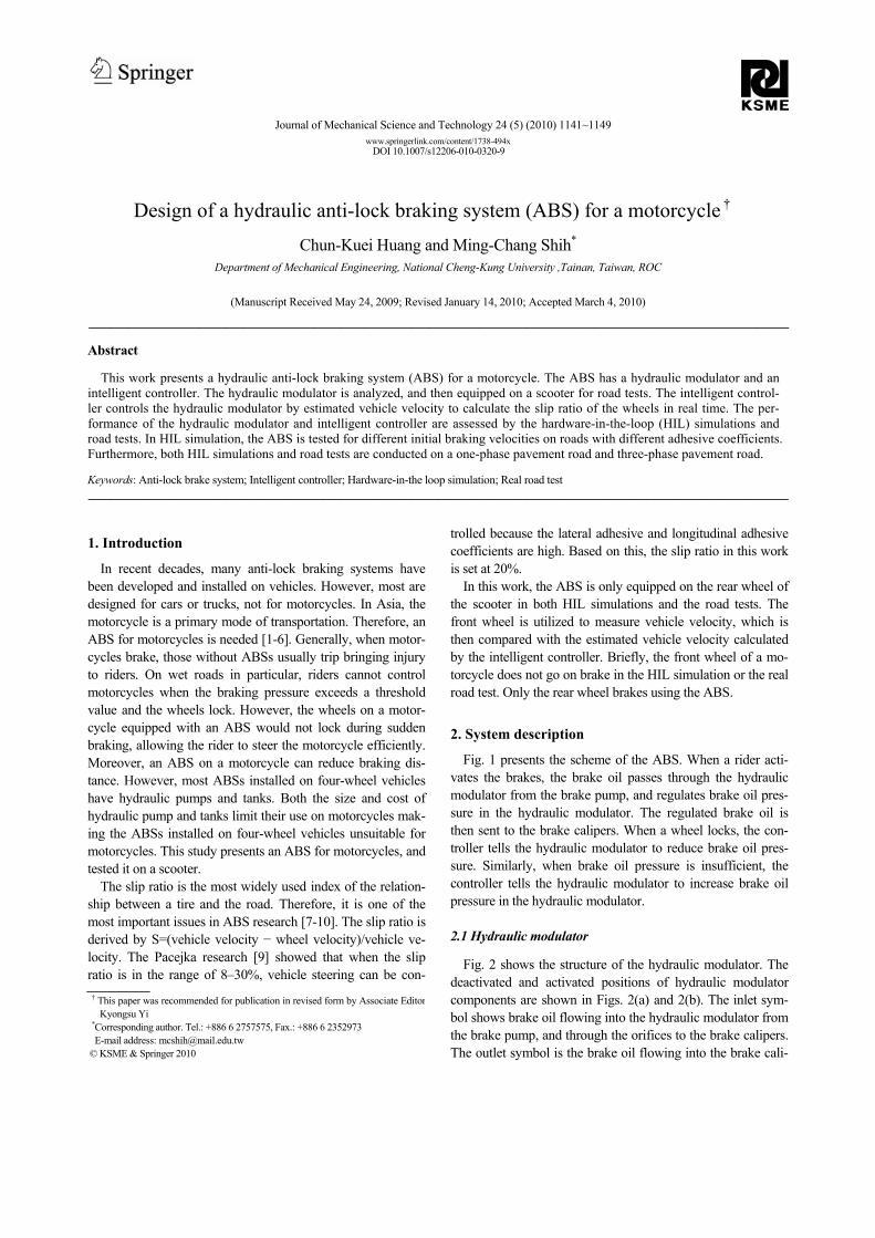
Fig. 2 shows the structure of the hydraulic modulator. The deactivated and activated positions of hydraulic modulator components are shown in Figs. 2(a) and 2(b). The inlet sym-bol shows brake oil flowing into the hydraulic modulator from the brake pump, and through the orifices to the brake calipers. The outlet symbol is the brake oil flowing into the brake cali-

† This paper was recommended for publication in revised form by Associate EditorKyongsu Yi

*Corresponding author. Tel.: +886 6 2757575, Fax.: +886 6 2352973 E-mail address: [email protected]

© KSME & Springer 2010

1142 C.-K. Huang and M.-C. Shih / Journal of Mechanical Science and Technology 24 (5) (2010) 1141~1149

pers from the hydraulic modulator. When the hydraulic modu-lator is deactivated, a rider can brakes a motorcycle in the usual manner, as long as motorcycle velocity is not too fast for the ABS or oil pressure does not cause the wheel to lock.

When the ABS is deactivated, the position of the spool is as shown Fig. 2(a). If brake pressure exceeds the target value calculated by the controller, the controller sends signals to the stepping motor and the spool is raised simultaneously by the motor as shown in Fig. 2(b). At this moment, brake oil from the brake pump is separated by the hydraulic modulator. The volume of Chamber D, which is between the spool and the bottom case, is increases; thus, oil brake pressure in the brake calipers decreases. That is, the controller can reduce brake pressure by increasing the volume of chamber D or can in-crease brake pressure by reducing the volume of chamber D. Briefly, the controller regulates the volume of chamber D such that the brake pressure in the calipers conforms to the target pressure.

The target pressure is calculated by the intelligent controller. When motorcycle velocity is zero and the ABS is not in use, the spool in modulator returns to its initial position [Fig. 2(a)]. The cylinder barrel is made by Teflon, which can lower the friction force when the spool is moving.

Generally, when an ABS is installed on a car, the brake

pedal will vibrate when the hydraulic modulator adjusts brak-ing pressure. For motorcycles, this vibration can cause a driver to lose control of the brake handle; thus, this vibration must be prevented. The hydraulic modulator in this study obstructs the brake oil out of the orifice by the spool [Fig. 2(b)]. When the hydraulic modulator is regulated, oil pressure from the brake pump and brake calipers are isolated; therefore, a rider will not feel vibrations from the brake handle during emergency brak-ing.

2.2 Mathematical analysis

Fig. 3 shows the relationship of the modulator, dynamics, and controller. In this section, the mathematical analyses of brake pump and ABS modulator are presented in 2.2.1 and 2.2.2. Section 2.2.3 discusses the mathematical model of vehi-cle dynamics and wheel dynamics. Section 2.2.4 presents the tire model. All these mathematical models were used in the simulation.

2.2.1 Brake pump

The dynamics of brake pump can be derived by

0( )m m m m m m mF A P P C X M x− ⋅ − − ⋅ = ⋅ && (1)

2 ( )m d p m sQ C A P Pρ

= ⋅ − (2)

0

m mm

mo m

V QPV V

β β= =&

& (3)

where mA and mX are the cross-section area and the dis-placement of the piston in brake pump, mC is the damping ratio, mP is the brake pressure in the brake pump, moV is the initial volume of mV , and pA is the area of the throttle in the brake pump.

Fig. 1. Scheme of the ABS.

(a) Inactivated (b) Operating

1. Motor 2. Upper case 3. Bottom case 4. Spool 5. Cylinder barrel Fig. 2. Structure of the hydraulic modulator.

Fig. 3. Scheme of a motorcycle.

Fig. 4. Mathematical symbols of brake pump.

C.-K. Huang and M.-C. Shih / Journal of Mechanical Science and Technology 24 (5) (2010) 1141~1149 1143

2.2.2 ABS modulator

Fig. 5 shows the mathematical symbols of the spool and cyl-inder barrel in the hydraulic modulator.

Oil flow rate aQ from the brake pump to the hydraulic modulator is

12 ( )a d s aQ C A P Pρ

= ⋅ ⋅ − (4)

where, sP is the oil pressure from the brake pump, aP is oil pressure in the volume aV , 1A is the cross-section area of orifice A , and ρ is the mass density.

Flow rates bQ and cQ are defined as

22 ( )b d a bQ C A P Pρ

= ⋅ ⋅ − (5)

32 ( )c d b cQ C A P Pρ

= ⋅ ⋅ − (6)

where, bP and cP are oil pressure in the volume bV and the volume cV , dC is the discharge coefficient, and. 2A and

3A are the cross-section area of orifice B and C . Therefore, the derivatives of pressure aP , bP and cP are

derived by a a

a be

V dPQ Qdtβ

− = (7)

b bb c

e

V dPQ Qdtβ

− = (8)

0 4c c c

c ce

dV V dPQ V V A Xdt dtβ

= + = + ⋅ (9)

where, eβ is the bulk modulus, and bV is the volume be-tween the upper case and the cylinder barrel. The volume cV is the total volume of chamber D and the caliper as shown in Fig. 2(b). X defines the movement of the spool, and 4A is the cross-section area of the spool.

2.2.3 Vehicle and wheel dynamics

In this work, the motorcycle is run in a straight line without camber or steer angle. Fig. 6 shows the force condition on the vehicle and the wheels. The vehicle model can be described as follows:

int

int

( ) /

( ) /f b G w w

r b G w w

N M g L F H F H L

N M g L F H F H L

= ⋅ ⋅ + ⋅ − ⋅

= ⋅ ⋅ − ⋅ + ⋅ (10)

where the subscripts f and r represent the front and the rear axle, respectively; N is the normal force of each wheel; M is the total mass of the motorcycle and rider; L is the distance between the front and rear wheel. aL and bL are the distance from the center of gravity to the front axle and the rear axle; wF is the longitudinal wind load equals 20.15 vV⋅ [5], vV is the vehicle velocity and the inertial force is defined as int w f rF M a F F F= ⋅ = − + + . The damping ratio and stiff-ness of the suspension system and the effects of rider postures are ignored. In Fig 6(b), the wheel dynamic equation is

t bI T Tω⋅ = −& (11) where I is the moment of inertia, and ω is the angular ve-locity. cbb PKT ⋅= is the brake torque, where bK is the tor-que gain and cP is oil pressure in the caliper. RFT it ⋅= is the torque from the tire force, where iF is the longitudinal force and R is the radius of the wheel [5]. 2.2.4 Tire model

Tire models [8-10] can be used to analyze the adhesive force between a tire and road. Many studies have attempted to develop a mathematical formula for tire, and it has two major groups. One group comprises the theoretical models based on tire construction. Another uses experimental results to define the parameters of tire models. In this work, the Pacejka ‘magic formula tire model’ is adopted. As the motorcycle run in a

Fig. 5. Mathematical symbols of hydraulic modulator.

　 (a)

(b)

Fig. 6. Force condition on the vehicle and the wheels.


straight line, the lateral forces from the tire are ignored. The longitudinal adhesive coefficient is defined as follows:

i iF N µ= ⋅ ,i f r= (12)

sin( arctan{ [arctan( )]})

i i

i

D C B S E B SB S

µ = ⋅ ⋅ ⋅ − ⋅

− ⋅ (13)

where

max 1 1D C Vµ= + ⋅ (14)

2 32 arcsin( ) ln(1 )s

vC C C VDµ

π= + ⋅ + ⋅ (15)

4 5 6tan{ / exp[ /(1 )]}s vC C C C VBC D C D

+ += =

⋅ ⋅ (16)

71tan( / 2 )

tan ( )m

vm m

B S CE C VB S B S

π−

⋅ −= + ⋅

⋅ − ⋅ (17)

8 9 vf C C V= + ⋅ (18)

iS is the slip ratio, maxµ is the maximum value of µ , and mS is the shifted slip ratio when the peak maxµ occurs. The

parameters 1C ~ 9C are derived from the Pacejka model [9].

3. Controller design

Fig. 7 shows the block diagram of motorcycle, which in-clude the proposed hydraulic modulator, controller, vehicle dynamics, wheel dynamics, and the tire model. The control-ler has pressure control logic and a sliding-mode controller.

The pressure control logic uses the pressure in the brake ca-lipers )(kPc and the angular velocity of wheel )(kω as commands, then determines the value of target brake pressure

refP . Target brake pressure is defined as the standard value of pressure in brake calipers. Moreover, the sliding-mode con-troller causes the pressure in brake calipers to track the target brake pressure. Section 3.1 defines the pressure control logic and Section 3.2 discusses the sliding-mode controller.

3.1 Pressure control logic

Fig. 8 shows the block diagram of pressure control logic. The pressure control logic has a velocity-estimated logic and a fuzzy controller.

First, the velocity-estimated slip ratio )(~

kSr is determined by the velocity estimation logic, which uses the angular veloc-ity )(kω and the braking pressure in calipers )(kPc as its inputs, by the following equations:

( ) _ ( )r r rS k S ref S K∆ = − % (19) ( ) ( ) ( 1)c cP k P k P k∆ = − − (20)

where refSr _ is the standard value of the slip ratio defined at 0.2.

Then, )(kSr∆ and )(kP∆ are sent to the fuzzy controller and the value of )(1 kPa is determined. Therefore, the target brake pressure can be determined by

0( ) ( )ref aP k P P k= + (21)

1( ) ( 1) ( )a a aP k P k P k= − + (22) where 0P is initial pressure, which can make the spool ob-struct the brake oil from brake pump move fast when ABS is operating. In this study, it is set at 25 bar. The velocity estima-tion logic is introduced in Section 3.1.1, and the parameters of fuzzy controller are discussed in Section 3.1.2.

Fig. 7. Block diagram of motorcycle with the ABS.

Fig. 8. Block diagram of pressure control logic.


3.1.1 Velocity estimation logic

In the ABS controller design, slip ratio is the most impor-tant factor in determining whether a wheel is locked, because tire longitudinal force (braking force) and lateral force (han-dling force) are related to slip ratio. If the controller wants to adjust the slip ratio, wheel angular velocity and vehicle veloc-ity must be measured in real time. However, vehicle velocity is not easily measured on real cars. Thus, the control rules on automobiles mostly use angular acceleration of wheels com-pared to threshold values, as Wu has done previously [11]. Lu [5] also presented a controller for a motorcycle, which uses vehicle acceleration for the controller command. In his ex-periment, vehicle acceleration was measured by an acceler-ometer and the controller calculated the target brake pressure. However, accelerometer measurements are easily impacted by noises of signal. Additionally, error of integral nonlinearity, or floating voltage of the zero point also influence the calculation of the vehicle velocity. Therefore, those controllers did not use the slip ratio as their command because vehicle velocity can-not be easily measured by the accelerometer on real car. In this study, the proposed velocity estimation logic calculates the slip ratio on a real motorcycle without an accelerometer.

The velocity estimation logic is applied to estimate vehicle velocity and to calculate the slip ratio in real time. From Eq. (11), the wheel dynamics are defined as

cbrbt PKRFTTI ⋅−⋅=−=⋅ω& . According to this equation, the moment of inertia I and wheel radius R are constants, and brake torque gain bK is considered a constant value in the different ranges of pressure value. The controller measures braking pressure cP in the brake calipers and wheel angular velocity ω using sensors. Therefore, the longitudinal adhe-sive force rF can be calculated. Similarly, the longitudinal adhesive force of another wheel fF can be calculated using this equation. Thus, vehicle acceleration can be determined by Newton’s law:

( ) /x r wa F F F M= + + (23) where M and wF represent the total mass and the longitudi-nal wind load, respectively (Section 2.2.3). Furthermore, vehi-

cle velocity can calculated by taVVv ⋅+= 0 , where 0V is the initial velocity. Based on this, the estimated slip ratio can be determined.

3.1.2 Fuzzy controller

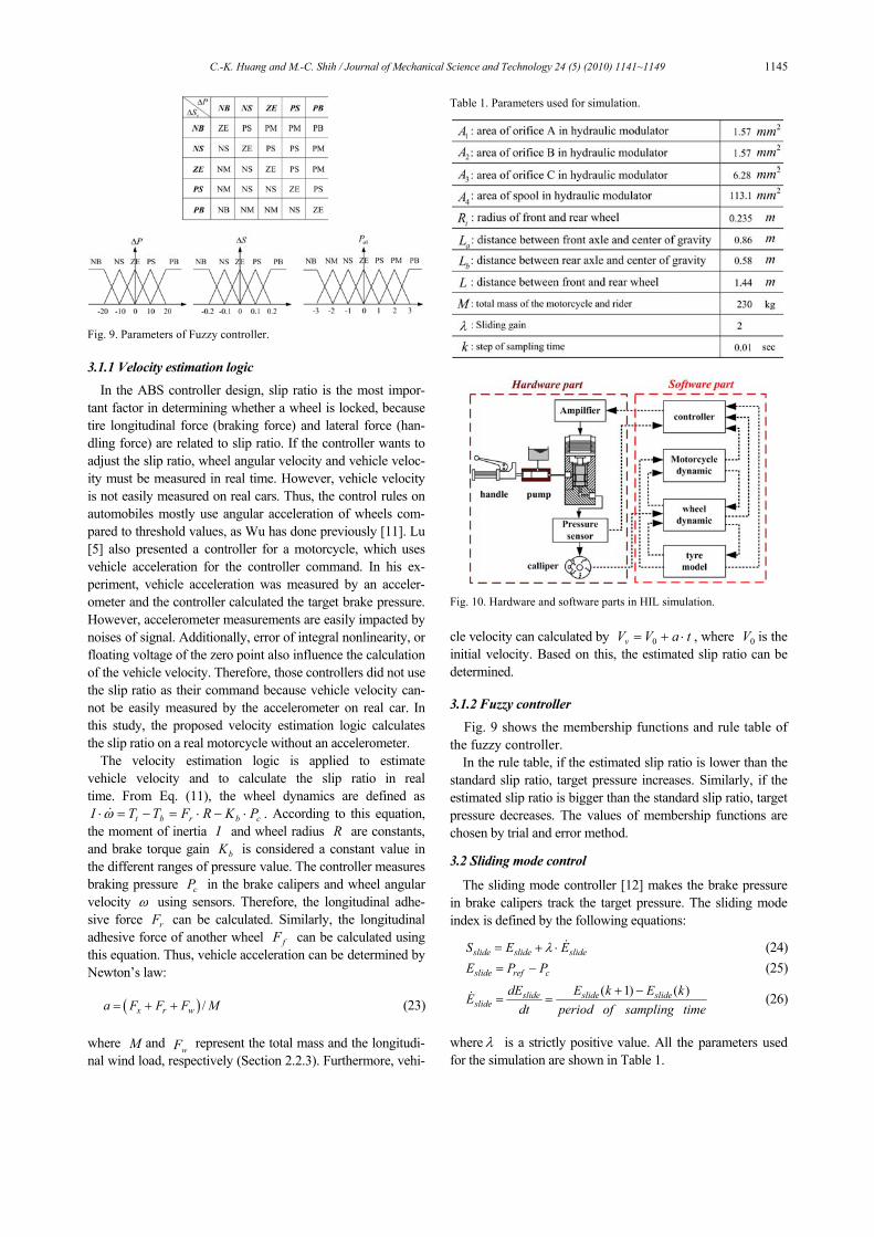
Fig. 9 shows the membership functions and rule table of the fuzzy controller.

In the rule table, if the estimated slip ratio is lower than the standard slip ratio, target pressure increases. Similarly, if the estimated slip ratio is bigger than the standard slip ratio, target pressure decreases. The values of membership functions are chosen by trial and error method. 3.2 Sliding mode control

The sliding mode controller [12] makes the brake pressure in brake calipers track the target pressure. The sliding mode index is defined by the following equations:

slide slide slideS E Eλ= + ⋅ & (24)

slide ref cE P P= − (25) ( 1) ( )slide slide slide

slidedE E k E kE

dt period of sampling time+ −

= =& (26)

where λ is a strictly positive value. All the parameters used for the simulation are shown in Table 1.

Fig. 9. Parameters of Fuzzy controller.

Table 1. Parameters used for simulation.

Fig. 10. Hardware and software parts in HIL simulation.


4. Hardware-in-the-loop (HIL)

Hardware-in-the-loop is a test method, in which real measurements of the physical hardware replace the mathe-matical model for a particular hardware during simulation [13]. Simulation via HIL is widely used in many studies, such as those on engine dynamics [14, 15] or motorcycle dynamics [16]. The purpose of using HIL simulation in this study is to simulate the motorcycle run on different adhe-sive coefficient roads and dangerous situations such as high speed travel of a motorcycle. Fig. 10 shows the hardware and software used in HIL simulations. The hardware com-prises a brake handle, brake pump, hydraulic modulator, brake calipers, and pressure sensor. The software comprises the controller, motorcycle dynamics, wheel dynamics, and tire model.

The HIL simulation results can be divided into two sections: the one-phase pavement road test which is discussed in Sec-tion 4.1, and the three-pavement road test, which is road test on three different pavements conditions discussed in Section 4.2.

4.1 One-phase pavement road test

In this section, motorcycle braking is tested with different initial velocities on a road with a constant adhesive coefficient and constant initial velocity on two roads with different adhe-sive coefficients.

4.1.1 Different initial velocities road tests

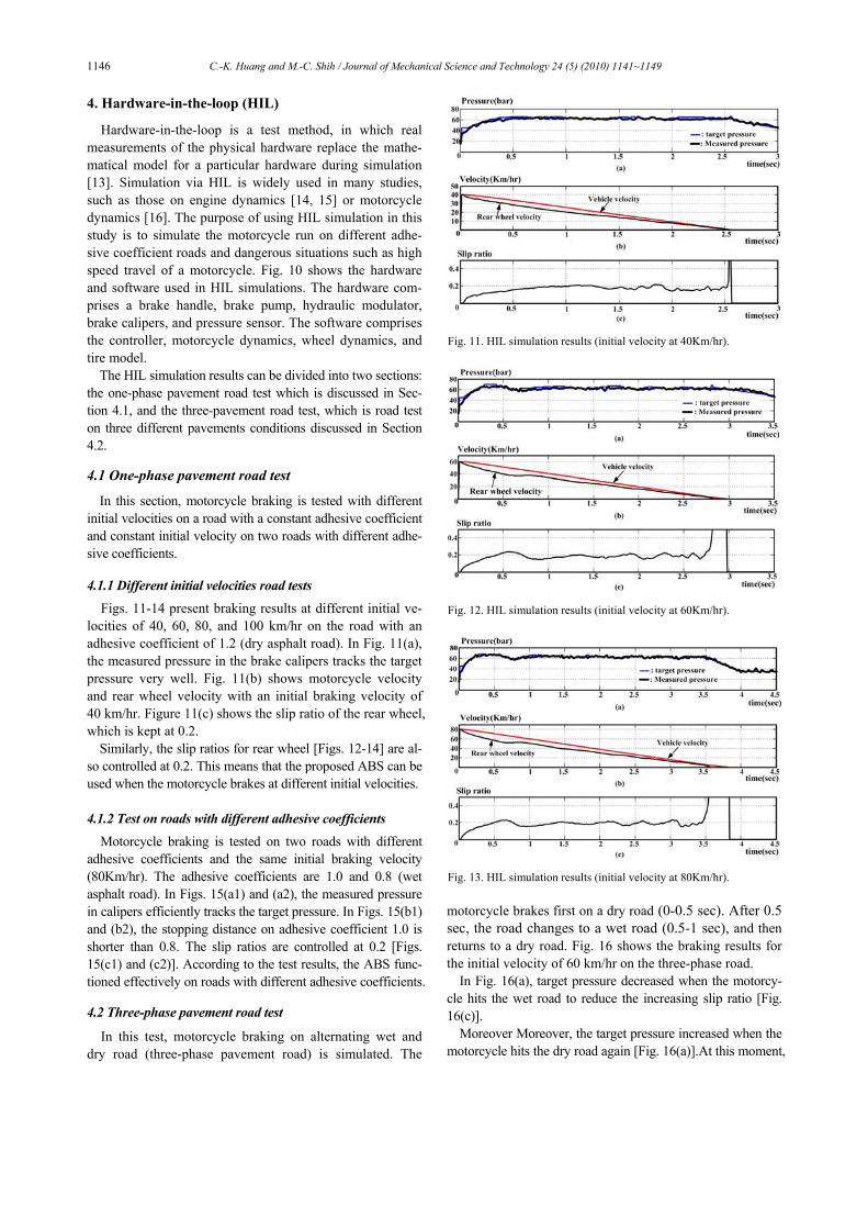
Figs. 11-14 present braking results at different initial ve-locities of 40, 60, 80, and 100 km/hr on the road with an adhesive coefficient of 1.2 (dry asphalt road). In Fig. 11(a), the measured pressure in the brake calipers tracks the target pressure very well. Fig. 11(b) shows motorcycle velocity and rear wheel velocity with an initial braking velocity of 40 km/hr. Figure 11(c) shows the slip ratio of the rear wheel, which is kept at 0.2.

Similarly, the slip ratios for rear wheel [Figs. 12-14] are al-so controlled at 0.2. This means that the proposed ABS can be used when the motorcycle brakes at different initial velocities.

4.1.2 Test on roads with different adhesive coefficients

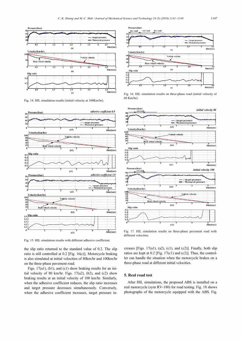
Motorcycle braking is tested on two roads with different adhesive coefficients and the same initial braking velocity (80Km/hr). The adhesive coefficients are 1.0 and 0.8 (wet asphalt road). In Figs. 15(a1) and (a2), the measured pressure in calipers efficiently tracks the target pressure. In Figs. 15(b1) and (b2), the stopping distance on adhesive coefficient 1.0 is shorter than 0.8. The slip ratios are controlled at 0.2 [Figs. 15(c1) and (c2)]. According to the test results, the ABS func-tioned effectively on roads with different adhesive coefficients. 4.2 Three-phase pavement road test

In this test, motorcycle braking on alternating wet and dry road (three-phase pavement road) is simulated. The

motorcycle brakes first on a dry road (0-0.5 sec). After 0.5 sec, the road changes to a wet road (0.5-1 sec), and then returns to a dry road. Fig. 16 shows the braking results for the initial velocity of 60 km/hr on the three-phase road.

In Fig. 16(a), target pressure decreased when the motorcy-cle hits the wet road to reduce the increasing slip ratio [Fig. 16(c)].

Moreover Moreover, the target pressure increased when the motorcycle hits the dry road again [Fig. 16(a)].At this moment,

Fig. 11. HIL simulation results (initial velocity at 40Km/hr).




the slip ratio returned to the standard value of 0.2. The slip ratio is still controlled at 0.2 [Fig. 16(c)]. Motorcycle braking is also simulated at initial velocities of 80km/hr and 100km/hr on the three-phase pavement road.

Figs. 17(a1), (b1), and (c1) show braking results for an ini-tial velocity of 80 km/hr. Figs. 17(a2), (b2), and (c2) show braking results at an initial velocity of 100 km/hr. Similarly, when the adhesive coefficient reduces, the slip ratio increases and target pressure decreases simultaneously. Conversely, when the adhesive coefficient increases, target pressure in-

creases [Figs. 17(a1), (a2), (c1), and (c2)]. Finally, both slip ratios are kept at 0.2 [Fig. 17(c1) and (c2)]. Thus, the control-ler can handle the situation when the motorcycle brakes on a three-phase road at different initial velocities.

5. Real road test

After HIL simulations, the proposed ABS is installed on a real motorcycle (sym RV-180) for road testing. Fig. 18 shows photographs of the motorcycle equipped with the ABS. Fig.


Fig. 15. HIL simulation results with different adhesive coefficient.

Fig. 16. HIL simulation results on three-phase road (initial velocity of 60 Km/hr).

Fig. 17. HIL simulation results on three-phase pavement road with different velocities.


18(a) and (b) show side view and back view of the motorcycle. Auxiliary wheels are installed on either side of the motorcycle to prevent collapse when the rear wheel locks during the test. The auxiliary wheels are installed higher than the front and rear wheels and do not touch the ground; thus, their influence can be ignored. Fig. 18(c) presents a photograph of the hy-draulic modulator. Fig. 18(d) present photographs of the con-trol box.

Figs. 18(e) and (f) present photographs of the device used to measure front and rear wheel angular velocities. The front wheel velocity is the measured velocity in the real road test. Section 5.1 discusses experimental results of the estimated vehicle velocity. Section 5.2 shows experimental results of the real road test. 5.1 Estimated vehicle velocity test

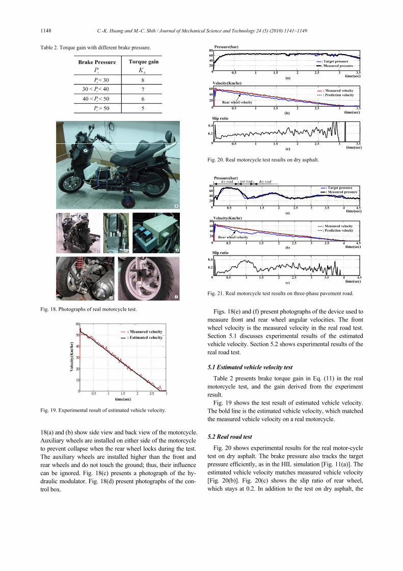
Table 2 presents brake torque gain in Eq. (11) in the real motorcycle test, and the gain derived from the experiment result.

Fig. 19 shows the test result of estimated vehicle velocity. The bold line is the estimated vehicle velocity, which matched the measured vehicle velocity on a real motorcycle. 5.2 Real road test

Fig. 20 shows experimental results for the real motor-cycle test on dry asphalt. The brake pressure also tracks the target pressure efficiently, as in the HIL simulation [Fig. 11(a)]. The estimated vehicle velocity matches measured vehicle velocity [Fig. 20(b)]. Fig. 20(c) shows the slip ratio of rear wheel, which stays at 0.2. In addition to the test on dry asphalt, the

Table 2. Torque gain with different brake pressure.

Fig. 18. Photographs of real motorcycle test.

Fig. 19. Experimental result of estimated vehicle velocity.

Fig. 20. Real motorcycle test results on dry asphalt.

Fig. 21. Real motorcycle test results on three-phase pavement road.


ABS was also tested on the three-phase pavement road. Fig. 21 shows the test results. The target pressure decreases when the motorcycle is on the wet road, and increases when the motorcycle touches the dry road [Fig. 21(a)]; the slip ratio is kept at 0.2 [Fig. 21(c)].

6. Conclusions

This work designs a hydraulic modulator, and an intelligent controller for an ABS. All of these are verified via HIL simu-lation and motorcycle tests. The proposed hydraulic modulator was easily fabricated. A distinct advantage is the absence of vibrations from the brake handle when the hydraulic modula-tor is in operation.

The HIL simulation results show that the hydraulic modula-tor and controller can keep the slip ratio at 0.2 with different initial braking velocities or under different adhesive coeffi-cients. In the real motorcycle experiment, the estimated vehi-cle velocity is the same as the measured vehicle velocity.

According to the experimental results, the braking action of the motorcycle can safely operate on both wet and dry roads.

Acknowledgment

This research was supported by the National Science Coun-cil Taiwan, ROC (NSC97-2221-E-006-052-MY2) which is greatly appreciated by the authors.

References

[1] M. Kato, T. Matsuto, K. Tanaka, H. Ishihara, T. Hayashi and W. Hosoda, Combination of antilock brake system (ABS) and combined brake system (CBS) for motorcycles, SAE., 960960 (1996) 1284-1291.

[2] A. Strichland and K. Dagg, ABS braking performance and steering input, SAE special publications, 980240 (1998) 57-64.

[3] F. M Georg, F. G. Gerard and C. Yann, Fuzzy Logic Con-tinuous and Quantizing Control of An ABS Braking System, SAE., 940830 (1994) 1033-1042.

[4] N. Miyasaki, M. Fukumoto, Y. Sogo and H. Tsukinoki, Antilock brake system (M-ABS) based on the friction coef-ficient between the wheel and the road surface, SAE special publications, 900207 (1990) 101-109.

[5] C. Y. Lu and M. C. Shih, Application of the Pacejka Magic Formula Tyre Model on a Study of a Hydraulic Anti-Lock Braking System for a Light Motorcycle, Vehicle System Dy-namics, 41(6) (2004) 431-448.

[6] M. Sugai, H. Yamaguchi, M. Miyashita, T. Umeno and K. Asano, New Control Technique for Maximizing Braking Force on Antilock Braking System, Vehicle System Dynam-ics, 32 (1999) 299-312.

[7] B. Ozdalyan, Development of A Slip Control Anti-lock Braking System, International Journal of Automotive Tech-nology, 9(1) (2008) 71-80.

[8] H. Dugoff, P. S. Fancher and L. Segel, An analysis of tire

traction properties and their influence on vehicle dynamic performance, Proceedings of the International Automobile Safety Compendium, Brussels, Belgium, SAE., 700377 (1970) 1219-1243.

[9] H. B. Pacejka, Tire and Vehicle Dynamics, Society of Automotive Engineers, Netherlands, (2002).

[10] R. S. Sharp and M. Bettella, Tyre shear force and moment description by normalization of parameters and the magic formula, Vehicle system dynamics, 39 (1) (2003) 27-56.

[11] M. C. Wu and M. C. Shih, Simulated and Experimental Study of Hydraulic Anti-Lock Braking System Control Us-ing Sliding-Mode PWM Control, Mechatronics, 13 (4) (2003) 331-351.

[12] Y. K. Chin, W. C. Lin, W. C. Sidlosky, M. Rule, S. Spar-schu and S. Mark, Sliding mode ABS wheel slip control, proceedings of the American control conference, Chicago, (1992) 1-8.

[13] S. J. Lee, Y. J. Kim and K. Park, Development of Hard-ware-In-the-Loop Simulation System and Validation of its Vehicle Dynamic Model for Testing Multiple ABS and TCS Modules, 7th International Symposium on Advanced Vehicle Control, (2004) 833-838.

[14] C. F. Lin, C. Y. Tseng and T. W. Tseng, A hardware-in-the-loop dynamics simulator for motorcycle rapid controller proto-typing, Control Engineering Practice, 14 (2006) 1467-1476.

[15] D. Bullock, B. Johnson, R. B. Wells, M. Kyte and Z. Li, Hardware-in-the-loop simulation, Transportation Research Part C 12 (2004) 73-89.

[16] C. W. Hong and C. C. Chen, Dynamic performance simula-tion of a continuously variable transmission motorcycle for fuzzy autopilot design, ImechE., (1997) 477-490.

Ming-Chang Shih is currently a Distin-guished University Professor of Me-chanical Engineering, National Cheng-Kung University, Taiwan. He received his B.S. and M.S. from the National Cheng-Kung University in 1973 and 1977, respectively. He received his Dr.-Ing. degree from the Technische

Hochschule Aachen in Germany. His current research in-cludes Pneumatic Nano-Position Control, Energy saving in hydraulic control system, Anti-lock brake System and Active Suspension system of vehicle.

Chun-Kuei Huang is currently a Ph.D. student of Mechanical Engineering, National Cheng-Kung University, Tai-wan. He received the Master’s degree from Department of Mechanical and Electro-Mechanical Engineering of the Sun Yat-Sen University in 2005. His research focuses on the tire model, and

the dynamic characteristics and the anti-lock brake system of motorcycle.

Design of a hydraulic anti-lock braking system (ABS… · Design of a hydraulic anti-lock braking...

Documents

Transcript of Design of a hydraulic anti-lock braking system (ABS… · Design of a hydraulic anti-lock braking...