Design and Implementation of Object Classifier based on...

Abstract

Design and Implementation of Object

Classifier based on Color and Shape

ECE 4600 Group Design Project

Group 16

Prepared By Atif Muhammad Bowen Shi Chinmai Managoli Milind Patel

Faculty Advisor

Dr. Sherif Sherif Associate Professor

March 9th, 2018

Abstract

i

Abstract

The goal of this project was to integrate shape and color detection capabilities and

implement a working assembly line-type model that sorts objects. Objects are placed at the start of

the conveyor belt and are automatically sorted when they reach the end of the belt. A color sensor

and a camera are connected to a Raspberry Pi computer and are fed the computer color and image

data from objects on the conveyor belt. The Raspberry Pi then processes this data and controls two

motors which assist in the transportation of objects and their sorting process. The color sensor

communicates with the Raspberry Pi using I2C communication interface. The camera relays data

to the computer over the dedicated CSI interface. The first motor is used to control the movement

of the conveyor belt while the second motor is used to implement the sorting process.

The report details the three major components in the project which are hardware, electric

circuitry and motors, and image processing. The hardware section describes the changes made to

the conveyor belt to interface it with the Raspberry Pi computer by adding a rotational DC motor

to turn the belt and a positional DC motor to sort the objects coming from conveyor belt. The

section also covers the placement of the camera and color sensor to detect objects effectively. The

circuitry and motors section explains the circuits designed to supply the appropriate voltage levels

to control the motors from the Raspberry Pi. Finally, the image processing section explains the

techniques used to determine the shape and color of different objects.

Contributions

ii

Contributions

The project was broken down into 5 sections: Hardware, Supporting Circuit, Image

Processing, Color Sensor Programming, and Integration and Testing. The contributions of each

member have been highlighted with bullet points in table 1.

Table 1: Contributions

Ati

f M

uh

amm

ad

Bo

wen

Sh

i

Ch

inm

ai M

anag

oli

Mil

ind

Pat

el

Hardware

Prototype Design and Modification

Prototype Implementation

Supporting Circuit

Motor Circuit Design

Motor Circuit Implementation

PCB Design and Implementation

Image Processing

Shape Detection using PC

Shape Detection using Raspberry Pi Computer

Integration with Camera

Color Sensor Programing

Color Sensing

Sensor Range Testing

Integration and Testing

Motors Integration with Raspberry Pi

Sensor Integration with Raspberry Pi

Final Program Flow Design and Testing

Report Writing

Acknowledgements

iii

Acknowledgements

A big thanks to our advisor, Dr. Sherif Sherif, for supporting us throughout the project, providing

valuable guidance, educating us about image processing techniques and being patient with us all

the way.

We would like to thank Mr. Daniel Card, for his invaluable advice and assistance he provided us

in the electrical section of our project.

A huge thanks to Ms. Aidan Topping for reviewing all our documents, answering our endless

questions and providing valuable feedback when it came to technical communications.

A big thanks to our colleague, Mr. Mujtaba Jalil, for his advice and technical guidance throughout

the project.

We would like to thank Mr. Sinisa Janjic and the late Ken Biegun for handling all our orders.

A huge thanks to Mr. Zoran Trajkoski for playing a vital role in our hardware implementation.

We would like to thank Dr. Derek Oliver for his feedback on our logbooks.

Table of Content

iv

Table of Content

ABSTRACT .......................................................................................................................................... I

CONTRIBUTIONS .............................................................................................................................II

ACKNOWLEDGEMENTS .............................................................................................................. III

TABLE OF CONTENT..................................................................................................................... IV

LIST OF FIGURES ........................................................................................................................... VI

LIST OF TABLES ............................................................................................................................ VII

NOMENCLATURE ....................................................................................................................... VIII

CHAPTER 1 - INTRODUCTION ...................................................................................................... 1

1.1 BACKGROUND .............................................................................................................................. 1

1.2 OVERVIEW ................................................................................................................................... 2

1.3 SCOPE ........................................................................................................................................... 3

Parameters for Success ..................................................................................................... 3

CHAPTER 2 - DESIGN AND IMPLEMENTATION ...................................................................... 4

2.1 CONVEYOR BELT MODIFICATION ................................................................................................. 4

2.2 SORTING SYSTEM ......................................................................................................................... 5

2.3 CAMERA AND SENSOR .................................................................................................................. 6

2.4 PROTOTYPE .................................................................................................................................. 7

CHAPTER 3 - DC MOTORS AND SUPPORTING CIRCUITY .................................................... 8

3.1 DC MOTOR................................................................................................................................... 8

3.2 CIRCUITRY TO CONTROL DC MOTOR ........................................................................................... 9

3.3 SERVO MOTOR ........................................................................................................................... 19

Modification of the Servo Motor .................................................................................... 20

3.4 POWER ....................................................................................................................................... 21

CHAPTER 4 - IMAGE PROCESSING ........................................................................................... 22

4.1 IMAGE CAPTURE......................................................................................................................... 23

4.2 CAMERA PARAMETERS ............................................................................................................... 24

ISO .................................................................................................................................. 24

Brightness ....................................................................................................................... 24

Table of Content

v

Contrast ........................................................................................................................... 24

Exposure Mode ............................................................................................................... 24

Resolution ....................................................................................................................... 24

Saturation ........................................................................................................................ 25

Sharpness ........................................................................................................................ 25

Shutter Speed .................................................................................................................. 25

4.3 I2C COMMUNICATION ................................................................................................................. 26

Using Color Filters to Remove Noise ............................................................................. 26

Removal of Background Noise ....................................................................................... 28

Grayscaling, Blurring and Edge Filter ............................................................................ 29

Canny Edge Detector [15] [16] ....................................................................................... 30

Raemer-Douglas-Peuker (RDP) Algorithm to Detect Shape from External Contour ..... 32

CHAPTER 5 - PROGRAM FLOW .................................................................................................. 33

5.1 OUTLINE ..................................................................................................................................... 33

5.2 LIBRARIES .................................................................................................................................. 34

CHAPTER 6 - CIRCUIT IMPLEMENTATION ............................................................................ 35

6.1 PROTOTYPING BOARD ................................................................................................................. 35

6.2 PCB FABRICATION ..................................................................................................................... 36

6.3 DESIGN CONSIDERATIONS. ......................................................................................................... 36

CHAPTER 7 - CONCLUSION ......................................................................................................... 38

7.1 FUTURE WORK ........................................................................................................................... 38

REFERENCES ................................................................................................................................... 40

APPENDIX A ...................................................................................................................................... 43

APPENDIX B ...................................................................................................................................... 44

List of Figures

vi

List of Figures

Figure 1-1 Project Flowchart ................................................................................................... 2

Figure 2-1 : Conveyor Belt Modification ................................................................................. 4

Figure 2-2 Object Sorting ........................................................................................................ 5

Figure 2-3 Camera and Sensor Placement ............................................................................... 6

Figure 3-1 Current Controlling Switch Circuit (closed) ........................................................ 12

Figure 3-2 Current Controlling Switch Circuit (open) ........................................................... 13

Figure 3-3 Active Low Voltage Circuit Open Switch ............................................................ 15

Figure 3-4 Active Low Voltage Circuit Closed Switch ......................................................... 16

Figure 3-5 Motor’s internal capacitor discharging ................................................................. 17

Figure 3-6 PWM: 6 Volts, 3% Duty Cycle ............................................................................ 18

Figure 3-7 Output Voltage at Motor Terminal ....................................................................... 19

Figure 3-8 Modified Servo Motor .......................................................................................... 20

Figure 4-1 : Shape Detection Process .................................................................................... 22

Figure 4-2 Camera and Sensor Setup ..................................................................................... 23

Figure 4-3 (a) Blue (b) Green (c) Orange (d) Yellow Colored Objects Captured Automatically

by the Camera Based on Signals from the Color Sensor ....................................................... 25

Figure 5-1 Program Flow Diagram ........................................................................................ 33

Figure 6-1 Circuit Implemented on Prototyping Board ......................................................... 35

Figure 6-2 (a) Fabricated PCB (b) PCB with Components Soldered .................................... 36

Figure 6-3 Frequency and Current Parameters Generated by Eagle ...................................... 37

Figure 6-4 Thick Wire Trace.................................................................................................. 37

Figure 0-1 Overall Hardware Implementation ....................................................................... 44

Figure 0-2 Sorting Bins and Switch ....................................................................................... 45

Figure 0-3 Raspberry Pi Mounted .......................................................................................... 45

List of Tables

vii

List of Tables

Table 1: Contributions ............................................................................................................. ii

Table 2 H-Bridge Logic table ................................................................................................ 20

Table 3 RGB Ranges for Different Colored Objects ............................................................. 29

Table 4 Color Sensor Data ..................................................................................................... 43

Nomenclature

viii

Nomenclature

CAD Computer Aided Design

DC Direct Current

EM Electromagnetic

GHz Giga Hertz

GPIO General Purpose Input/Output

I2C Inter Integrated Circuit

k Kilo

M Mega

MHz Mega Hertz

PCB Printed Circuit Board

PWM Pulse Width Modulation

RDP Raemer Douglas Peuker

RGB Red, Green, Blue

SCL Serial Clock Line

SDA Serial Data

SPI Serial Peripheral Interface

ULP User Language Program

Introduction

1

Chapter 1 - Introduction

1.1 Background

Object sorting and shape detection are used in many industries, such as in the food

production industry, where it is used to maintain quality standards by ensuring that all manufactured

goods look exactly the same. For example, image processing is used to look for defects in processed

foods as part of the quality control procedure [1]. Another example is the use of image processing

to validate product specifications like date/time and expiry [2]. Image processing can also be used

in sorting processes like waste sorting, which is often done manually in garbage processing and

recycling plants [3].

Assembly lines are at the epicentre of the manufacturing industry and the industrial

revolution [4]. Assembly lines ease the task of processing and packaging products in almost every

industry. Many of today’s assembly lines are automated to improve efficiency and productivity in

industries. One of the early examples of assembly line automation is that of the Ford motor

company [5].

RGB color sensors work on the principle that every color is composed of the three primary

colors – red, blue and green. Color sensors are used in many sorting applications on assembly and

production lines, along with image processing techniques. Image processing is the use of computer

algorithms to process digital images for various applications [6]. Advanced image processing is

used in traffic surveillance to monitor traffic patterns and traffic violations [7]. It is also used by

self-driving autonomous cars to scan for traffic signs [8]. Image processing techniques can be

applied on different objects to determine their contour. When an image of an object is captured,

each pixel in the image has an RGB level associated with the color of that pixel. This information

can be used to distinguish the object from its background and determine the object’s contour.

Introduction

2

1.2 Overview

The main goal of this project was to integrate color and shape sensing capabilities of an

object on a single device. The device was implemented using a combination of color sensor, image

processing with an external camera and a conveyor belt. The objects were classified based on their

colors and shapes. A readily available conveyor belt was modified as an alternative to building the

working model from raw materials. In order to control the sorting process, appropriate DC motors

were selected. External circuits were designed to control the DC motors from the Raspberry Pi

computer. The detection and sorting process are outlined in the flowchart shown in figure 1-1.

Figure 1-1 Project Flowchart

Objects

Camera and

RGB Color

Sensor

Raspberry Pi

Controller

Board

Circuitry

DC Rotational

Motor

DC Servo

Motor

Conveyor Belt

Slider Bar for

Classification

Introduction

3

1.3 Scope

Shapes of simple, basic objects were determined so that they could be sorted using an

assembly line-like prototype, as a proof of concept. A Raspberry Pi computer was used to carry out

image capture, processing and control of the subsequent sorting mechanism. The assembly line was

implemented on a modified conveyor belt with the help from the mechanical tech shop.

Parameters for Success

For the project to be considered a success, the following parameters were set:

1. The size of the entire working model was to be less than 80 inches in length by 20 inches

in width by 30 inches in height.

2. The power consumption of all the components used was to be under 40 watts.

3. Each object would have to be sorted within 15 seconds from the time it landed on the

conveyor belt.

4. The shape and color of the object was to be determined by the Raspberry Pi computer in

under 7 seconds.

5. A total of 4 or more different colors and 3 or more different shapes had to be determined.

Design and Implementation

4

Chapter 2 - Design and Implementation

The aim of this project is to identify different objects based on shape and color and sort them.

A conveyor system was implemented to achieve this task. The conveyor system relayed the objects

to be sorted to their respective sorting piles. Conveyor systems are used in various industries for

food processing, manufacturing, package processing, etc. [9].

2.1 Conveyor Belt Modification

An off-the-shelf alternative shown in figure 2-1 (a) was used as an alternative to building

the conveyor belt from raw materials. The belt was automated so that it could be controlled by the

Raspberry Pi computer. The belt had an axle on each end, which aided in the belt’s movement. A

DC motor was attached to one of the axles as shown in figure 2-1 (b). The DC motor was controlled

by the Raspberry Pi computer. The rotation of the motor was then automated using signals from

the computer.

Figure 2-1 : Conveyor Belt Modification

(a) (b)


5

2.2 Sorting System

A slide was designed to move objects into their appropriate sorting container once they

reached the end of the conveyor belt. The slide acted as a feed to four sorting containers, where

objects were classified by color or shape. The movement of the four sorting containers was

controlled by a rotating DC servo motor. The appropriate sorting container, in which the object was

to be dropped, moved directly under the end of the slide so that the object landed right into the

container. There were practical difficulties in maintaining the orientation of the containers with

respect to the end of the slide over multiple trials. Consequently, the motor was designed to move

to a fixed reference position after each object was classified. The reference position was determined

by a push-button switch. When the motor moved the containers to one end, it resulted in the pushing

of this button which signalled the Raspberry Pi computer. This point was taken as the reference

position. The motor moved the containers to this reference position after each object was classified.

The slide is shown in figure 2-2 (a) and the switch which was used to orient the containers with

respect to the slide is shown in figure 2-2 (b).

Figure 2-2 Object Sorting

(a) (b)


6

2.3 Camera and Sensor

The design uses an RGB color sensor and a camera to detect color and shapes of various

objects. A wooden post was designed to house the Raspberry Pi computer, camera and RGB color

sensor. The optimal distance between the conveyor belt and the camera for effective shape detection

was determined to be roughly 8cm. A small hole was drilled on top of the wooden post so that the

camera could have a direct line-of-sight with the conveyor belt and any object that went directly

under the camera on the belt. Data from the color sensor was used in the shape detection process.

Consequently, the color of the object was to be determined before the object’s image was captured

and processed. The color sensor also had to be very close to the objects on the conveyor belt for

accurate readings. As the average height of the objects was about 1cm, the color sensor was

designed to sit at a height of 1.5cm from the conveyor belt. This resulted in the objects being only

0.5cm away from the color sensor at the time of detection. The setup is shown in figure 2-3.

Figure 2-3 Camera and Sensor Placement


7

2.4 Prototype

When an object is placed on the moving conveyor belt, it first goes under the RGB color

sensor. The color sensor detects the object, sends its RGB data to the Raspberry Pi computer and

stops the conveyor belt after a certain fixed delay. This lands the object directly under the camera

for image capture. The conveyor belt remains stopped until the shape of the image is successfully

determined. Once the shape and color information of the object have been identified, Raspberry Pi

computer resumes movement of the conveyor belt. At the same time, the second motor brings the

appropriate sorting bin to the mouth of the slide. Once the objects lands in its designated bin, the

sorting bins move back to their reference position. The conveyor belt continues to rotate so that the

cycle can be repeated for the next object. The time taken per object to go to its respective sorting

bin is under twelve seconds. See appendix B for additional images of the prototype.

DC Motors and Supporting Circuity

8

Chapter 3 - DC Motors and Supporting Circuity

This chapter details the DC motors and the supporting electrical circuitry that was designed to

interface them with the Raspberry Pi computer.

3.1 DC Motor

A rotational DC motor was used to move the conveyor belt. DC motors contain a stator

and a rotor. DC motors are also referred to as permanent magnet direct current motors. This is due

to the fact that the stator contains a fixed permanent magnet producing a uniform and stationary

magnetic flux inside the motor. The armature consists of electrical coils wound around a metal

which produce a North and South Pole. When current flows through these coils, it produces an

electromagnetic field that generates a rotational movement [10].

To control the movement of the conveyor belt, a Pulse Width Modulation (PWM)

controlled rotational motor was used. The PWM was used to control the speed and movement of

the motor by regulating the amount of voltage across the motor terminals. To control the motor

with a PWM, a series of on-off pulses of varying duty cycles were applied. The duty cycle was

used to control the speed as well as the direction of rotation of the motor [11].

To operate the conveyor belt, a motor with slightly higher than normal torque rating was

required. Operating voltage of the motor was 4.8 – 6 volts, with stall torque of 125.2 – 141.9 oz.in.

The PWM pulses only serve the purpose of initiating the rotation of the motor. Stopping the PWM

did not stop the rotation of the motor. As a result, the PWM signal could not be used to control the

motor. The motor could be stopped by cutting off the power supply altogether. Hence, the control

of the motor was achieved by controlling the power supply of the motor. At an operating voltage

of 6 volts, the motor had a steady state current consumption of ~0.17 amperes. Therefore, an

external motor controlling switch circuit was designed to turn the motor on and off. The switch


9

circuit was designed to supply a steady state current of 0.17 amperes and voltage drop of about 6

volts.

3.2 Circuitry to Control DC Motor

As stated in section 3.1, a switch circuit was to be designed to control the motor. The motor

operated at a voltage range of 4.8-6 volts. A 6 volt DC power supply was chosen to satisfy the

voltage requirements. The switch was designed to be controlled by the GPIO pins on the Raspberry

Pi computer which supplied ~3.3 volt signals. The switch was designed by using transistors as

switches and amplifiers.

Transistors are three terminal active devices that can serve two purposes: switching and

amplification. Bipolar transistors can operate in three different regions: [18]

1) Active region – The transistor operates as an amplifier. Emitter current IC can be defined

by

IC = β*IB (3.1)

Where β = Current Gain and IB = Base Current

2) Cut Off region – Transistor is OFF and IC ≈ 0

3) Saturation region – Transistor is ON IC = Saturation current

A PNP transistor was used in series with a small 1 Ohm resistor with high power rating to

control the supply voltage to the motor. In the simulation stage, the motor was modelled by a 33

ohm resistor. The motor resistance was calculated as follows:

Voltage Supply = 6V

Motor Current = 0.18 A

Let R1 = Effective Resistance of Motor

V = I R

R1 = V/I = 6V/0.18A

R1 = 33.33 Ω (3.2)


10

An NPN transistor circuit was used in parallel to account for any leakage currents from the

current control circuit. Therefore, the maximum required current by using a small 1 Ohm resistor

at the PNP transistor side could be pulled. On the NPN side, a 1K Ohm resistor (R4) was connected

at the emitter of the NPN transistor to limit the current drain from the source. This current drain at

the NPN transistor could be controlled by changing the value of R4.

From the Raspberry Pi, a 3.3 volt GPIO Pin was connected to the base of the NPN

transistor. When a “High” signal i.e. 3.3 volts was supplied from the controller board, the transistor

operated in its active region. Figure 3-1 shows the voltage drop at the collector terminal of about

2.64 volts. The drop from the base to the collector of the amplifier was 0.65 volts. Current at the

emitter branch,

Ie1 = 2.64V/ 1000 Ω= 2.6mA (3.3)

According to the bipolar transistor property, current at the emitter is equal to the sum of the base

current and collector current i.e. Ie = Ic + Ib. As current in the base was very small, the

approximation, Ib1 ≅ 0 amperes, was used. The current in the emitter is given by

Ie1 = Ic1 = 2.6mA (3.4)

In the circuit, the base terminal of the PNP transistor was connected to the collector terminal of the

NPN transistor. Therefore,

Ib2 ≅ Ic1 = 2.6mA (3.5)

Using Ic = β*Ib, Where β = 60 to 80 for PNP 2907, we get

Ic ≅ 171mA

Ic ≅ Ie ≅ 171mA (3.6)

The DC motor required 4.8 – 6 volts with ~0.17 amperes in the steady-state to operate smoothly.

The voltage at the R2 which represents the motor is equal to


11

V = 171mA*33.33 Ω = 5.62V (3.7)

This satisfied this requirement.

Once the switch is opened, i.e. “Low” signal at the GPIO, the transistor goes into the cut-

off region. Hence, Ic1 = 0 since it is in cut-off mode. Also, Vb1 = 0, therefore, with the voltage drop

across the internal diode, Ve1 = ~ -0.65 volts.

Ie1 = -0.65V/1000 Ω = 0.65mA (3.8)

Ie1 was neglected as it was a very small value compared to the active region current.

Ib2 = Ic1 = 0.65mA (3.9)

Ic2 = β* Ib2 = 43.75mA (3.10)

This current was not enough to drive the motor. The PNP transistor acted as a switch for the input

current of the motor. Controlling the high and low signal from the controller board gave full control

of the rotation of the motor by controlling the amount of current that flowed through it. Hence, this

circuit acted as a current controlling switch. Figure 3-2 shows the simulation design when 3.3 volt

supply is disconnected.


12

Figure 3-1 Current Controlling Switch Circuit (closed)


13

Figure 3-2 Current Controlling Switch Circuit (open)

The signal level of the PWM was to be the same as the voltage rating of the motor. The

Raspberry Pi GPIO pin supplied 3.3 volt signals. Using the bipolar NPN transistor, an external

Active Low Voltage control circuit was designed to provide ~6 volt signals to the DC motor.

A 3.3 volt GPIO pin from the Raspberry Pi was connected in series with a 500 Ohm resistor

to the transistor base. A 6 volt source was supplied to the collector in series with a 5.6k Ohm

resistor. The internal resistor at the PWM terminal of the motor was measured to be in the Mega

Ohms range. Therefore, a 1M Ohm resistor was used to represent the PWM terminal of the motor

in parallel with the NPN transistor for simulation. The 5.6k Ohm resistor acted as a voltage drop to

control the voltage supply to the motor.


14

When a 3.3 volt signal was supplied to the base, the transistor operated in active mode.

Approximately all the current flowed through the transistor and no current flowed towards the

motor due to high resistance. This resulted in a very small voltage drop across the 1M ohm resistor,

~1.53 volt, which was not enough to initiate rotation of the motor. Once the 3.3 volt signal was

disconnected, the voltage at the base of NPN transistor dropped to zero and the transistor operates

in cut-off region. Therefore, the current at the collector was zero and all the current flowed to the

PWM port. The PWM calculation is shown below:

Using voltage division,

Voltage at the 1M Ohm resistor,

Vpwm = 6V x 1𝑀Ω

5.6𝑘Ω+1𝑀Ω = 5.96V (3.11)

Therefore, a voltage drop of ~5.96 volts was achieved at the PWM terminal. The circuit

was designed to be active-low, since it operated in the active region at a lower logic level, which

resulted in the rotation of the DC motor. Figure 3-3 and figure 3-4 show the design and results of

Active Low voltage circuit.


15

Figure 3-3 Active Low Voltage Circuit Open Switch


16

Figure 3-4 Active Low Voltage Circuit Closed Switch

The designed circuit was implemented on a prototype board and tested. Even though circuit

provided 5.74 volts to the motor terminal, the motor did not operate. It was observed that there was

indeed some power being supplied to the motor since the motor vibrated. However, the motor did

not rotate. The voltage drop across the motor terminals was measured with an oscilloscope. At the

same time, the current flowing into the motor was measured. It was observed that the motor pulled

a surge current when it was turned on. A surge of current went through the inner capacitor to charge

it and the resistor defined the charging time of the capacitor. After multiple trials, the peak voltage

was measured to be ~800 milli volts and it took ~90 micro seconds to charge the capacitor. The

lowest voltage was at ~400 milli volts with a charging time of ~50 micro seconds. Figure 3-5 shows

the results for 400 milli volt peak represent the voltage across the capacitor and the resistor is

0.1Ohm.

I = V/R = 0.4V/0.1 Ω = 4A (3.11)


17

Figure 3-5 Motor’s internal capacitor discharging

Time it took to charge the capacitor was about ~50 micro seconds. From this data, the

approximate value of the inner capacitor of the motor was calculated using decaying exponential

method. Below is the calculation for charge of the capacitor and the capacitance value of the motor.

Q = ʃ (I * e^ ((-t/τ)) dt), integrate from 0 < t < ∞

I = 4A, τ = 50 us

Q = 0.2x10-3 C

Using capacitance C = Q/V

C1 = (0.2𝑥10−3) 𝐶

6 𝑉

C1 = 30 x 10-6 F (3.12)

Using the same approach, the highest approximate capacitance value was also calculated and

found to be C1 = 0.13 x 10-3 farad. To charge the inner capacitor C1 of the motor, a larger capacitor

C2 was connected in parallel with the motor. The circuit first charged C2 which in turn provided the

surge current to C1. A capacitance C2 = 9.4x10-3 farad was used in parallel with the motor. A resistor


18

was also connected in series with C2 to provide the required time constant. The time constant was

necessary to immediately turn off the motor once the power was shut off.

The Current Controlling Switch, Active Low Voltage and RC2 circuit, in parallel with the

motor, were built on a breadboard and tested to operate and control the DC motor using PWM

signals from the Raspberry Pi computer. Once a 3.3 volt signal was supplied to the base of the NPN

transistor, the motor received its rated voltage and current, and started rotating. When the 3.3 volt

signal was disconnected from the Raspberry Pi computer, the output voltage at the motor terminal

dropped to ~0 volts and the motor became stationary. The motor could be successfully controlled

using signals from the Raspberry Pi computer. Figure 3-6 shows the output 6 volt PWM signal with

3% duty cycle and 60 hertz frequency when logic low level signal was provided to the base of the

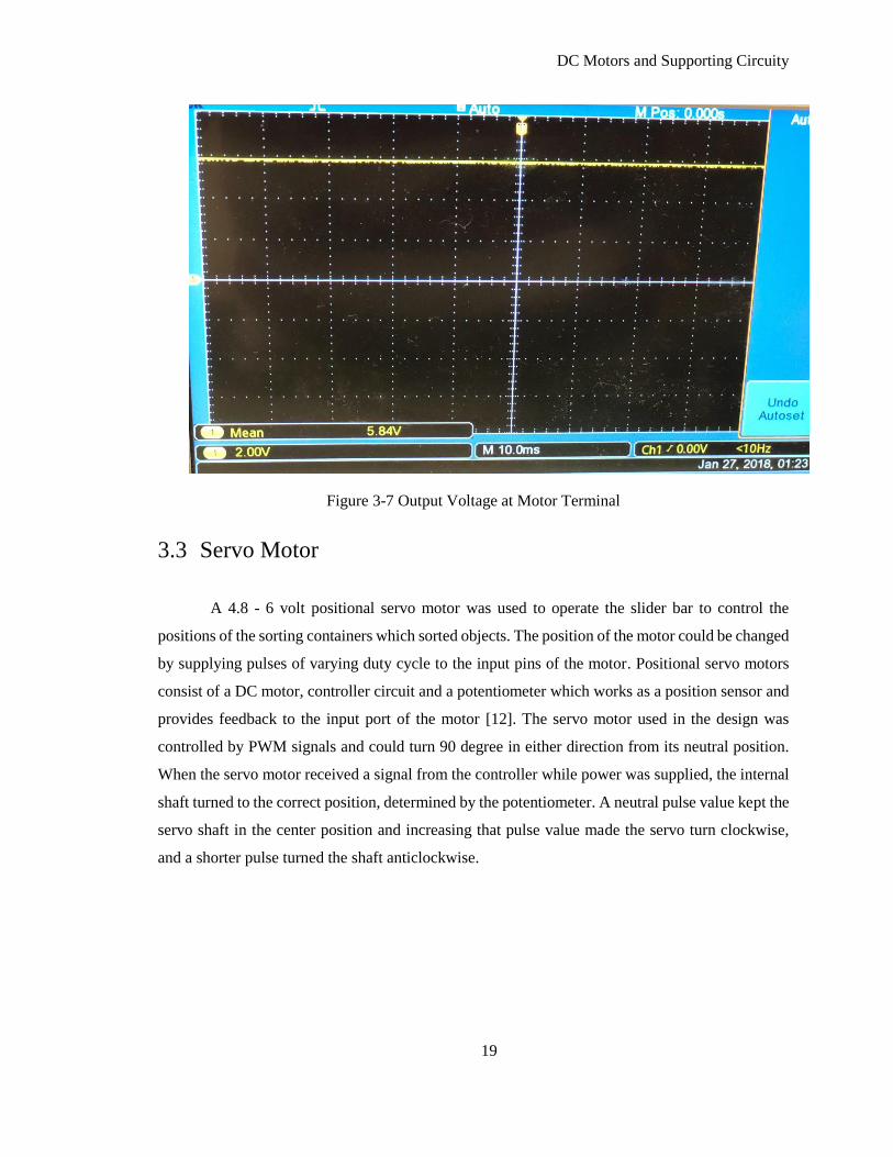
active low voltage circuit. Figure 3-7 represents the output voltage of the motor when 3.3 volt signal

was applied to the base of the current limiting circuit. This circuit was also implemented on the

prototyping board and PCB designs were made. Details of the prototyping board and PCB design

are explained in chapter 6 of this report.

Figure 3-6 PWM: 6 Volts, 3% Duty Cycle


19

Figure 3-7 Output Voltage at Motor Terminal

3.3 Servo Motor

A 4.8 - 6 volt positional servo motor was used to operate the slider bar to control the

positions of the sorting containers which sorted objects. The position of the motor could be changed

by supplying pulses of varying duty cycle to the input pins of the motor. Positional servo motors

consist of a DC motor, controller circuit and a potentiometer which works as a position sensor and

provides feedback to the input port of the motor [12]. The servo motor used in the design was

controlled by PWM signals and could turn 90 degree in either direction from its neutral position.

When the servo motor received a signal from the controller while power was supplied, the internal

shaft turned to the correct position, determined by the potentiometer. A neutral pulse value kept the

servo shaft in the center position and increasing that pulse value made the servo turn clockwise,

and a shorter pulse turned the shaft anticlockwise.


20

Modification of the Servo Motor

The design was improved to have a different sorting mechanism due to the limited rotation

of the positional servo motor. As a result, the feedback path of the positional motor was removed

to make it a fully rotational motor whose direction could be controlled with the help of two signals

that controlled an internal H-bridge. The logic table 3-1 of the servo is shown below:

Table 2 H-Bridge Logic table

Signal A Signal B Output

High Low Clockwise rotation

Low High Anticlockwise rotation

Low Low No operation

High High No operation

Figure 3-8 Modified Servo Motor

In table 3.1, high represents 6 volts and low represents 0 volts. The different logic level

combinations supplied to pins A and B of the servo motor resulted in either clockwise or anti-

clockwise rotation or no rotation at all as described in table 3.1. For example, when pin A was

6V

Signal A

Signal B

Ground


21

supplied with 6 volts and pin B was supplied 0 volts, the servo motor rotated clockwise. The

modified servo motor is shown in figure 3-8. The signal levels used to control the new modified

motor had to be the same as the input voltage level, which was 6 volts. Hence, a CE amplifier

similar to the active low voltage in figure 3-3 was used to amplify the signals coming from the

Raspberry Pi.

3.4 Power

The power consumption of each component in the model was measured. The motor that moved

the conveyor belt and the motor that moved the sorting bins consumed 1.1 watts of power each.

The Raspberry Pi computer powered the camera and color sensor. Hence, accounting for the

computer’s power consumption accounted for all other components. The Raspberry Pi’s power was

observed to peak at about 8 watts. The power never exceeded 8 watts.

When the motors were stationary, the circuitry still consumed some minimum power. The total

power losses in the stationary mode was measured to be ~0.65 watts. This was a very small amount

of power compared to the power consumption when the motors were being operated.

This resulted in a total power consumption to be less that 12 watts even in the worst case

scenario assuming about a 20% margin for error.

Image Processing

22

Chapter 4 - Image Processing

The following flowchart in figure 4-1 outlines the process by which object shapes are

determined:

Figure 4-1 : Shape Detection Process

Each step in the shape detection process is described in the following sections.

Image Processing

23

4.1 Image Capture

The color sensor and camera had been set up in such a way that the color sensor first

detected an object directly below it. The color sensor then paused the movement of the conveyor

belt after an appropriate delay such that the object stopped right below the camera. This was done

in order to get clear image capture and successful detection. Figure 4-2 shows the setup of the

camera and sensor.

Figure 4-2 Camera and Sensor Setup

The color sensor had four 16-bit data fields that it sent to the Raspberry Pi using the I2C

communication protocol – clear, red, green and blue, each ranging from 0 to 65535. The clear field

indicated how close an object was to the color sensor. In the case of the particular color sensor

being used, when there was no object under the sensor, the typical value for the clear field was

around 900 to 1000. The clear field jumped to a higher number ranging from 4000 to 35000 when

there was an object under the color sensor, depending on color and shape of the object. The

controller board stopped the movement of the conveyor belt 250 milli seconds after the color sensor

had detected an object, hence landing the object right under the camera for successful image

capture. Figure 4.3 shows sample images of objects captured by the camera.

Camera

Objects start moving

from this point

Objects first go under the color

sensor and stop right below the

camera after an appropriate delay

for clean image capture

Image Processing

24

4.2 Camera Parameters

The following camera parameters [13] were modified for optimal image capture:

ISO

ISO is a measure of the sensitivity of the image sensor. Generally, lower ISO values are

used when the camera is required to be less sensitive to light. Higher ISO settings are used in darker

conditions. The ISO can be set to any value between 0 and 1600. In our application, an ISO value

of 800 was used.

Brightness

The brightness level of the camera can be set to any value from 0 to 100. It indicates how

much white is mixed in the color. A brightness level of 70 was chosen for our application.

Contrast

Contrast in a camera is the scale of difference between black and white in images. The

Raspberry Pi camera’s contrast can be set to a value from -100 to +100. A contrast of +100 was

chosen in our project to have maximum contrast and effective edge detection.

Exposure Mode

The exposure of the camera can be set to auto, night, backlight, antishake, etc., or can even

be turned off. The exposure mode was set to ‘night’ to account for the dark color of the conveyor

belt and low-light conditions.

Resolution

The resolution of the image captured affected the size of the image captured. Higher

resolutions lead to better quality images but there was a trade-off with processing time. An optimal

resolution of 512 x 512 was used.

Image Processing

25

Saturation

Saturation indicates the amount of grey in a color. It could be set to a value between -100

and +100 on the Pi Camera. It was set to 0 for optimal performance.

Sharpness

The sharpness in an image indicates the amount of edge contrast. Maximum edge contrast

of +100 was chosen for our application.

Shutter Speed

The shutter speed of the camera was automatically determined by the auto-exposure

algorithm built into the Raspberry Pi camera.

Figure 4-3 (a) Blue (b) Green (c) Orange (d) Yellow Colored Objects Captured Automatically by

the Camera Based on Signals from the Color Sensor

(a) (b)

(c) (d)

Image Processing

26

4.3 I2C Communication

The TCS3472-5 light-to-digital converter, shown in figure 4-4, was used as a color sensor

in the design. It contained a 3x4 photodiode array. The Inter-Integrated Circuit (I2C) protocol allows

multiple digital integrated circuits or “slave” chips to communicate with one or more “master”

chips. In this case, the “slave” chip being the color sensor and the “master” being the Raspberry

Pi. It requires only 2 signal wires, SCL and SDA, and is only intended for short distance

communications. I2C is an asynchronous communication, meaning it does not need clock data to

be transmitted. The main advantage of using I2C over SPI and other synchronous communication

protocols is that it requires less number of pins. It is not intended for simultaneous sending and

receiving of data (full-duplex). [14]

Figure 4-4 Pin Diagram for Color Sensor TCS3472

Using Color Filters to Remove Noise

The object color was to be determined by using data from the red, green and blue (RGB)

data fields of the color sensor. When the clear field was triggered, the clear along with the RGB

values were recorded. It was observed that there was a direct correlation between the clear field

and the RGB values. A higher clear value was accompanied by higher value readings of red, green

and blue. Hence, the ratios of red-to-green, green-to-blue and red-to-blue were used to determine

object color. Figure 4-5 below shows typical ratios for different colored objects.

Image Processing

27

(a)

(b)

0

0.5

1

1.5

2

2.5

3

3.5

0 1 2 3 4 5 6

Rat

io

Trial Number

Red-to-Green

Orange Colored Objects

Blue Colored Objects

Green Colored Objects

Yellow Colored Objects

0

0.5

1

1.5

2

2.5

3

3.5

0 1 2 3 4 5 6

Rat

io

Trial Number

Green-to-Blue





Image Processing

28

(c)

Figure 4-5 Color ratios for different colored objects

Using the clear distinction that we had in the ratios for different colored objects, the colors

of the objects were determined. For the detailed recordings of the color sensor data for different

trials, see Appendix A.

Removal of Background Noise

Once the color of the object had been determined, the data was used to apply bit-wise

masking to the frame captured by the camera. This was done to filter out the background noise and

get an accurate shape prediction. Every color has a unique range of RGB values which can be

filtered from the rest of the image. Table 4-1 shows the RGB lower and upper limits for different

color objects used in this project. The RGB values range from 0 to 255.

0

1

2

3

4

5

0 1 2 3 4 5 6

Rat

io

Trial Number

Red-to-Blue





Image Processing

29

Table 3 RGB Ranges for Different Colored Objects

Lower Limit [R, G, B] Upper Limit [R, G, B]

Orange Color Object 185, 60, 0 220, 120, 55

Yellow Color Object 150, 150, 0 255, 255, 20

Blue Color Object 0, 0, 100 50, 100, 255

Green Color Object 0, 100, 0 90, 255, 100

Figure 4-6 shown below demonstrates an example of how the method described above can be used

to perform shape recognition. The small amount of noise in the image left after bitwise masking

can easily be eliminated.

Figure 4-6 Color Filter Applied on Image to get rid of most of the Background Noise.

Grayscaling, Blurring and Edge Filter

In order to process an image for shape detection, it was first converted into a grayscale

image. Then, a blur was applied on the image to get rid of the small amount of noise left over after

implementing the color filter. After removing the noise, the Canny edge detection filter was applied

to obtain the external contour of the object. Figure 4-7 shows the process described.

Image Processing

30

Canny Edge Detector [15] [16]

The Canny edge detector uses a multi-stage algorithm to detect edges in images. The Canny

edge detector has a low error rate and has almost no false edges. The distance between the edge

pixels detected and the real edge pixels is minimized and there is only one response per edge to

reduce running time. The edge detector first filters out any noise, usually with a Gaussian noise

filter. It then finds the intensity gradient of the image. It then removes pixels that are not considered

to be part of an edge. This leaves behind only thin lines in the image. The process of removing

these pixels is called non-maximum supression. The edge detector then uses a process called

Hysteresis which compares pixel gradients to an upper and a lower threshold to determine edges.

An algorithm similar to the Canny filter is the Sobel edge detector which uses a similar

methodology to detect edges in an image. Figure 4-8 shows the implementation of the Canny and

Sobel filters in the early stages of this design project on Matlab.

Figure 4-7 Obtaining the External Contour of the Object

Grayscale

Canny Edge Detector

Blurring

Image Processing

31

Figure 4-8 The Edge Detected Image of the Raspberry Pi Logo (a) Original (b) Canny and Sobel

Edge Detection

(a)

(b)

Image Processing

32

Raemer-Douglas-Peuker (RDP) Algorithm to Detect Shape from

External Contour

The RDP algorithm takes a curve which is composed of line segments and finds a similar

curve with fewer points. The approxPolyDP function in the OpenCV library uses this algorithm.

The approxPolyDP function approximates a curve or a polygon with another curve or polygon with

less vertices so that the distance between them is less or equal to the specified precision. Figure 4-

9 demonstrates the working of the RDP algorithm

.

Figure 4-9 The RDP algorithm has converted the original curve in (a) to a more simplified curve

with less number of vertices as shown in (b) [17]

(a)

(b)

Program flow

33

Chapter 5 - Program flow

The program that received data from the color sensor, captured images using the Raspberry Pi

camera, processed images and controlled the conveyor belt and sorting bins has been described in

this section.

5.1 Outline

The program described in figure 5-1 was written in python. The various libraries used in the

program have been described briefly in the following section.

Figure 5-1 Program Flow Diagram

Import required libraries

Define thread functions for

various processes

Execute thread

for color sensor

class

Setup Raspberry Pi GPIO pins

Execute thread

for image

processing class

Execute thread

for sorting class

Program flow

34

5.2 Libraries

Rpi Library was used to control the various GPIO pins on the Raspberry Pi computer. It was

used to set pin modes to input or output and to generate PWM signals for the conveyor belt’s DC

motor. The input mode pin was used to read the signal coming in from the push-button switch

which indicated the reference position of the sorting bins.

The smbus library was used to implement the I2C interface to read data from the color sensor.

The library accessed the I2C/dev interface on the Raspberry Pi. To implement this library, the host

kernel, which was the Raspberry Pi kernel, had to have I2C support, I2C device interface support

and a bus drive adapter.

The time library was used to measure time between certain events in the detection and sorting

process and set delays at various points in the program.

The PiCamera library provided a pure python interface to operate the Raspberry Pi camera

module. This library enabled image capture, video capture, setting camera parameters like

brightness, hue, saturation, and adding special effects to images like night, negative, snowy,

spotlight, etc.

The OpenCV library was used to process the images captured by the camera. It was a very

rich library with a variety of pre-defined methods that could be used for image and video

processing. In the project, it was used to resize images, convert RGB color images to grayscale,

apply blur to images to reduce noise, apply thresholding to binarize images, find contours in images

and apply edge detection methods. The library is very capable of even higher end applications like

face recognition and computer vision for artificial intelligence.

Large array operations necessary during image processing were carried out by the numpy

library.

Circuit Implementation

35

Chapter 6 - Circuit Implementation

This chapter describes the implementation of the circuit on a prototyping board as well as PCB

design.

6.1 Prototyping board

After designing the circuit on a breadboard, it was implemented on a plane prototyping board.

The circuit was developed for multiple functions i.e. current limiter for bidirectional DC motor and

active low voltage control for all motors. Figure 6-1 provided below shows the setup for

prototyping circuit.

Figure 6-1 Circuit Implemented on Prototyping Board


36

6.2 PCB Fabrication

To provide an efficient interface between the peripherals and the Raspberry Pi, a PCB was

fabricated. The goal was to minimize the extra space while maintaining the connection integrity of

the circuit. It also added a robustness feature to the system. Figure 6-2 represents the fabricated

PCB.

Figure 6-2 (a) Fabricated PCB (b) PCB with Components Soldered

6.3 Design Considerations.

The PCB was designed using Eagle CAD software. One major challenge was to ensure that

the PCB copper traces were large enough to handle the current requirement. Eagle CAD offers a

ULP script feature, which was used to calculate the required trace length and width for current

required. Even though the project did not require any high frequency communication through the

PCB, it was designed to operate with digital signals of frequencies as high as 1GHz. Figure 6-3

represents the measured data generated through Eagle.

Inputs

Outputs

Power Source


37

Figure 6-3 Frequency and Current Parameters Generated by Eagle

The second most important consideration was to handle current spikes at the start-up for

the DC motor. As discussed in chapter 3 the initial operation for DC motor required a current as

high as 0.8 amperes. To absorb the heat generated from the current spike and analog noise

generated from the surrounding electrical equipment along with thick power line traces, a ground

plane was integrated in to the PCB as shown in Figure 6-4. It not only dissipated heat properly

but also helped against the 60 hertz EM noise.

Figure 6-4 Thick Wire Trace

Thick Wire

Trace

Conclusion

38

Chapter 7 - Conclusion

The goal of this project was to implement a device that integrated color and shape sorting

capabilities on a single device. The project was broken down into hardware implementation, image

acquisition and processing, and electrical circuitry to interface the Raspberry Pi computer with

various peripheral devices. The hardware implementation relayed objects from one end of a

conveyor belt to another in order for the objects to be sorted according to their shape and color.

Performance metrics were set at the start of the project to determine the success or failure

of the project. The finished device could identify different object colors and shapes. It could sort

the objects based on either of these. In case of failure to detect shapes, the object colors would still

be identified. In the worst-case scenario, the conveyor belt would continued to relay the object and

the object would be sorted into a sorting container designated specifically for indeterminate objects.

The entire design had a power consumption of less than 12 watts. The prototype was capable of

detecting up to 4 different shapes and 4 different colors accurately in less than 12 seconds.

The allotted budget for the project was $400. The estimated cost of this project was

$241.03. The project was successfully implemented at a cost of $310.68. The project cost was

slightly above the estimate. This was because a PCB was implemented to control the motors. This

was over and above the performance goals set by the team at the start of the project.

7.1 Future Work

In future, the device can undergo more advanced development. One improvement it can have

is the capability to detect more shapes of higher complexity. Also, the feature to detect multiple

different shapes at the same time can be added. These features can put the device to some real

practical use, since not all shapes are simple in nature. Another improvement it can have is the

automation of the placing of objects on the conveyor belt. This will enable the device to be

integrated into a real assembly line in a manufacturing industry. This reduces human labour costs

since sorting tasks are often done manually by hand. Thirdly, material sensing capability can be

added on to the device which will open the doors for application of the device to many other

39

industries. The user-friendliness for all these aforementioned applications can be further enhanced

by adding a wireless control option with a graphical user interface for users to operate easily.

References

40

References

[1] Stemmer-imaging.co.uk. (2018). Cite a Website - Cite This For Me. [online] Available at:

https://www.stemmer-

imaging.co.uk/media/uploads/websites/documents/publications/Innovations-in-Food-

Technology-2011-08.pdf [Accessed 9 Mar. 2018].

[2] Stemmer-imaging.co.uk. (2018). Cite a Website - Cite This For Me. [online] Available at:

https://www.stemmer-

imaging.co.uk/media/uploads/websites/documents/applications/en_DE-Application-Kdorf-

Automation.pdf [Accessed 9 Mar. 2018].

[3] Hennepin.us. (2018). Cite a Website - Cite This For Me. [online] Available at:

https://www.hennepin.us/-/media/hennepinus/business/recycling-hazardous-

waste/documents/waste-sort-guide.pdf?la=en [Accessed 9 Mar. 2018].

[4] A Big Step Towards Fewer Steps. (2018). The Assembly Line and its Importance.

[online] Available at: https://hfordassemblyl.weebly.com/the-assembly-line-and-its-

importance.html [Accessed 9 Mar. 2018].

[5] Anon, (2018). [online] Available at: https://www.assemblymag.com/articles/91581-the-

moving-assembly-line-turns-100 [Accessed 9 Mar. 2018].

[6] En.wikipedia.org. (2018). Digital image processing. [online] Available at:

https://en.wikipedia.org/wiki/Digital_image_processing [Accessed 9 Mar. 2018].

[7] Ieeexplore.ieee.org. (2018). Scan - An application of advanced image processing technology

to traffic surveillance - IEEE Conference Publication. [online] Available at:

http://ieeexplore.ieee.org/document/1622828/ [Accessed 9 Mar. 2018].

[8] Pdfs.semanticscholar.org. (2018). Cite a Website - Cite This For Me. [online] Available at:

https://pdfs.semanticscholar.org/c5ae/ec7db8132685f408ca17a7a5c45c196b0323.pdf

[Accessed 9 Mar. 2018].

References

41

[9] En.wikipedia.org. (2018). Conveyor belt. [online] Available at:

https://en.wikipedia.org/wiki/Conveyor_belt [Accessed 9 Mar. 2018].

[10] Innovateus.net. (2018). What is DC Motor?. [online] Available at:

http://www.innovateus.net/innopedia/what-dc-motor [Accessed 9 Mar. 2018].

[11] ARTICLES, T., ARTICLES, I., ELECTRONICS, G., PROJECTS, C., MICRO, E., Lectures,

V., Webinars, I., Training, I., Search, P., DB, T., Tool, B. and Library, C. (2018). Pulse

Width Modulation | DC Motor Drives | Electronics Textbook. [online] Allaboutcircuits.com.

Available at: https://www.allaboutcircuits.com/textbook/semiconductors/chpt-11/pulse-

width-modulation/ [Accessed 9 Mar. 2018].

[12] Jameco.com. (2018). How Servo Motors Work. [online] Available at:

https://www.jameco.com/jameco/workshop/howitworks/how-servo-motors-work.html


[13] Picamera.readthedocs.io. (2018). 9. API - The PiCamera Class — Picamera 1.13

Documentation. [online] Available at: https://picamera.readthedocs.io/en/release-

1.13/api_camera.html [Accessed 9 Mar. 2018].

[14] Learn.sparkfun.com. (2018). I2C - learn.sparkfun.com. [online] Available at:

https://learn.sparkfun.com/tutorials/i2c [Accessed 9 Mar. 2018].

[15] En.wikipedia.org. (2018). Canny edge detector. [online] Available at:

https://en.wikipedia.org/wiki/Canny_edge_detector [Accessed 9 Mar. 2018].

[16] Docs.opencv.org. (2018). Canny Edge Detector — OpenCV 2.4.13.6 documentation. [online]

Available at:

https://docs.opencv.org/2.4/doc/tutorials/imgproc/imgtrans/canny_detector/canny_detector.h

tml [Accessed 9 Mar. 2018].

References

42

[17] En.wikipedia.org. (2018). Ramer–Douglas–Peucker algorithm. [online] Available at:

https://en.wikipedia.org/wiki/Ramer%E2%80%93Douglas%E2%80%93Peucker_algorithm


[18] Anon, (2018). [online] Available at: https://www.electronics-

tutorials.ws/transistor/tran_1.html [Accessed 9 Mar. 2018].

Appendix A

43

Appendix A

Color sensor data measurements

Table 4 Color Sensor Data BC

Appendix B

44

Appendix B

Images of the hardware implementation

Figure 0-1 Overall Hardware Implementation

Appendix B

45

Figure 0-2 Sorting Bins and Switch

Figure 0-3 Raspberry Pi Mounted

Design and Implementation of Object Classifier based on...

Documents

Transcript of Design and Implementation of Object Classifier based on...