DESIGN AND ANALYSIS OF FULLY MAGNETIC A Thesis …martins/cubesat/ACS/DanGuerrant_thesis... ·...
122
DESIGN AND ANALYSIS OF FULLY MAGNETIC CONTROL FOR PICOSATELLITE STABILIZATION A Thesis presented to the Faculty of California Polytechnic State University, San Luis Obispo In Partial Fulfillment of the Requirements for the Degree Master of Science in Aerospace Engineering by Daniel Vernon Guerrant June 2005
Transcript of DESIGN AND ANALYSIS OF FULLY MAGNETIC A Thesis …martins/cubesat/ACS/DanGuerrant_thesis... ·...

DESIGN AND ANALYSIS OF FULLY MAGNETIC
CONTROL FOR PICOSATELLITE STABILIZATION
A Thesis
presented to
the Faculty of
California Polytechnic State University, San Luis Obispo
In Partial Fulfillment
of the Requirements for the Degree
Master of Science in Aerospace Engineering
by
Daniel Vernon Guerrant
June 2005

ii
AUTHORIZATION FOR REPRODUCTION OF MASTER’S THESIS
I grant permission for the reproduction of this thesis in its entirety or any of its parts, without further authorization from me. _____________________________________ Signature _____________________________________ Date
iii
APPROVAL PAGE
TITLE: Design and Analysis of Fully Magnetic Control for Picosatellite Stabilization
AUTHOR: Daniel Vernon Guerrant DATE SUBMITTED: June, 2005 _____________________________________________________________________ Dr. Jordi Puig-Suari, Advisor and Committee Chair Date _____________________________________________________________________ Dr. Eric Mehiel, Committee Member Date _____________________________________________________________________ Dr. Clark Turner, Committee Member Date

iv
ABSTRACT
Design and Analysis of Fully Magnetic Control for Picosatellite Stabilization
Daniel Vernon Guerrant
This thesis explores the possibilities of achieving three-axis stability on a picosatellite using only
magnetic torquers for actuation. The problem is broken into two phases: detumbling and
stabilization. The first phase uses the B-dot algorithm to lower the spacecraft rotation to that of
the local magnetic field and only requires magnetometers for sensing the field. The algorithm
was found to be very resilient to high noise levels, inaccurately calibrated magnetometers, and
magnetorquer failure and performed very well even with initial velocities above 10 rpm. The
second phase implements a proportion and derivative feedback controller to achieve 10º-20º of
pointing accuracy. This algorithm required full knowledge of attitude and rates, and
requirements for potential sensors were explored. It was found to be stable even with extremely
low resolution and noisy sensors, albeit with an increase in pointing error. The algorithm was
also found to be functional with limited controllability under magnetorquer failure. Both
simulations include models of the hardware and the gravity gradient disturbance torque.
v
Table of Contents
Page
List of Tables ............................................................................................................................... viii
List of Figures................................................................................................................................ ix
Nomenclature................................................................................................................................. xi
1 INTRODUCTION .................................................................................................................. 1
2 THEORY AND BACKGROUND ......................................................................................... 2
2.1 CubeSat/PolySat ............................................................................................................. 2
2.2 Magnetic Torquing.......................................................................................................... 3
2.3 Modeling the Earth’s Magnetic Field ............................................................................. 4
2.4 Coordinate Reference Frames and Transformations....................................................... 4
2.4.1 The Body Frame ..................................................................................................... 5
2.4.2 The Inertial Frame................................................................................................... 5
2.4.3 The Orbital Frame................................................................................................... 5
2.4.4 Successive Quaternion Rotations............................................................................ 6
2.4.5 Transformation of Angular Rates ........................................................................... 7
2.5 The Equations of Motion ................................................................................................ 8
2.6 Attitude Disturbance Torques ......................................................................................... 8
2.6.1 Minimum Torquing Ability .................................................................................... 9
2.6.2 Magnetic ................................................................................................................. 9
2.6.3 Aerodynamic Drag.................................................................................................. 9
2.6.4 Gravity Gradient ................................................................................................... 10
2.6.5 Solar Pressure........................................................................................................ 10
vi
2.6.6 Summary ............................................................................................................... 11
2.7 Survey of the Field........................................................................................................ 11
2.7.1 B-dot Controller .................................................................................................... 12
2.7.2 Three-Axis Controller........................................................................................... 13
3 HARDWARE ....................................................................................................................... 14
3.1 Side and Front Panels.................................................................................................... 15
3.2 Magnetometers.............................................................................................................. 16
3.3 Magnetorquers .............................................................................................................. 17
4 ATTITUDE SIMULATION COMPONENTS..................................................................... 18
4.1 Orbit Propagator............................................................................................................ 18
4.2 Magnetic Field Estimation............................................................................................ 18
4.3 Disturbance Torques ..................................................................................................... 19
4.4 Hardware Models.......................................................................................................... 19
4.4.1 Magnetorquers ...................................................................................................... 19
4.4.2 Magnetometers...................................................................................................... 20
4.4.3 Other Possible Attitude Determination Hardware ................................................ 22
4.5 B-dot Detumbling Algorithm........................................................................................ 23
4.6 Three-Axis Control Algorithm ..................................................................................... 23
4.7 Computation.................................................................................................................. 25
4.8 Summary of Simulation Assumptions .......................................................................... 26
5 ATTITUDE SIMULATION RESULTS .............................................................................. 27
5.1 B-dot Detumbling ......................................................................................................... 28
5.1.1 Explanation of B-dot plots .................................................................................... 28
vii
5.1.2 Optimum Gain Determination .............................................................................. 29
5.1.3 Optimum Pulse Time Determination.................................................................... 35
5.1.4 Effect of Magnetometer Noise.............................................................................. 40
5.1.5 One and Two Torquers Out Performance............................................................. 46
5.1.6 CP2 Method vs. CP3 Method ............................................................................... 49
5.1.7 B-Dot Conclusions................................................................................................ 51
5.2 Three-Axis Control ....................................................................................................... 52
5.2.1 Explanation of Three-axis Plots............................................................................ 52
5.2.2 Optimum Gains Determination............................................................................. 54
5.2.3 Optimum Pulse Time Determination.................................................................... 60
5.2.4 Effect of Sensor Resolution .................................................................................. 64
5.2.5 Effect of Sensor Noise .......................................................................................... 69
5.2.6 One and Two Torquers Out Performance............................................................. 74
5.2.7 Commanding Different Quaternions..................................................................... 77
5.2.8 Commanding in the Orbital Frame ....................................................................... 79
5.2.9 Three-Axis Conclusions........................................................................................ 82
5.3 Comparison of B-dot and Three-Axis Controllers........................................................ 82
6 FUTURE WORK.................................................................................................................. 84
BIBLIOGRAPHY......................................................................................................................... 86
Appendix A: Magfd.m.................................................................................................................. 87
Appendix B: CP2 Magnetometer Calibration Data ...................................................................... 91
Appendix C: Orbit Propagation and Attitude Simulator .............................................................. 92

viii
List of Tables
Table 2.1: Worst Case Attitude Disturbance Torques ................................................................. 11
Table 5.1: Three-axis gain investigation...................................................................................... 60
Table 5.2: Results of Pulse Length Variation .............................................................................. 64
Table 5.3: Comparison of B-dot and three-axis algorithms......................................................... 83
Table B.1: Calibration data for CP2 flight panels........................................................................ 91
ix
List of Figures
Figure 2.1: The inertial and orbital frames ..................................................................................... 6
Figure 3.1: CP2 Engineering Model ............................................................................................. 14
Figure 3.2: CP2 side panel interior face....................................................................................... 15
Figure 3.3: CP2 side panel with HMC 1052 magnetometer highlighted..................................... 16
Figure 3.4: CP2 Side Panel with approximate torquer location................................................... 17
Figure 5.1: Ground track for 5 orbits ............................................................................................ 27
Figure 5.2: B-dot for 1.5 orbits with K = 17e4 and δt = 10sec..................................................... 30
Figure 5.3: B-dot for 1.5 orbits with K = 11e4 and δt = 10sec..................................................... 31
Figure 5.4: B-dot for 1.5 orbits with K = 8e4 and δt = 10sec....................................................... 32
Figure 5.5: B-dot for 1.5 orbits with K = 2e4 and δt = 10sec....................................................... 33
Figure 5.6: B-dot for 1 orbit with δt = 12 sec and ωo = 1 rpm ...................................................... 36
Figure 5.7: B-dot for 1.5 orbit with δt = 1sec and ωo = 14 rpm .................................................... 37
Figure 5.8: B-Dot Tip-off Velocity Performance ......................................................................... 38
Figure 5.9: B-dot for 1 orbit with δt = 2sec and ωo = 1 rpm ......................................................... 39
Figure 5.10: B-dot for 1 orbit with δt = 2sec, ωo = 7 rpm, σ = 20 bits.......................................... 41
Figure 5.11: B-dot for 2 orbits with δt = 10sec, ωo = 0.5 rpm, σ = 0 bits ..................................... 42
Figure 5.12: B-dot for 2 orbits with δt = 10sec, ωo = 0.5 rpm, σ = 2 bits ..................................... 43
Figure 5.13: B-dot for 2 orbits with δt = 10sec, ωo = 0.5 rpm, σ = 6 bits ..................................... 44
Figure 5.14: Noise level vs. average settling rates........................................................................ 45
Figure 5.15: B-dot for 1.5 orbits with δt = 10sec, ωo = 1 rpm, σ = 3 bits, torquer 1 inactive....... 47
Figure 5.16: B-dot, 1.5 orbits, δt = 10sec, ωo = 1 rpm, σ = 3 bits, torquers 1 and 2 inactive ....... 48
Figure 5.17: CP2 B-dot for 1 orbit with δt = 4 sec, ωo = 3 rpm, σ = 6 bits................................... 50

x
Figure 5.18: 3-axis, C1 = 4e-2, C2 = 3e-5, δt = 20sec, 5 orbits ..................................................... 55
Figure 5.19: 3-axis, C1 = 5e-2, C2 = 3e-5, δt = 20sec, 3 orbits ..................................................... 56
Figure 5.20: 3-axis, C1 = 2e-2, C2 = 1e-5, δt = 20sec, 5 orbits ..................................................... 57
Figure 5.21: 3-axis, C1 = 2e-2, C2 = 2e-5, δt = 20sec, 5 orbits ..................................................... 58
Figure 5.22: 3-axis, C1 = 4e-2, C2 = 3e-5, δt = 20sec, 5 orbits, 3º shutoff ................................... 59
Figure 5.23: 3-axis, C1 = 4e-2, C2 = 3e-5, δt = 17sec, 4 orbits, 3º shutoff ................................... 62
Figure 5.24: 3-axis, C1 = 4e-2, C2 = 3e-5, δt = 10sec, 5 orbits, 3º shutoff ................................... 63
Figure 5.25: 3-axis, C1 = 2e-2, C2 = 2e-5, δω = 1e-3 rad/s, δq = 0.01.......................................... 65
Figure 5.26: 3-axis, C1 = 4e-2, C2 = 3e-5, δω = 0.01 deg/s, δq = 0.01 ......................................... 66
Figure 5.27: 3-axis, C1 = 4e-2, C2 = 3e-5, δω = 1e-4 rad/s, δq = 0.5............................................ 67
Figure 5.28: 3-axis, C1 = 4e-2, C2 = 3e-5, δω = 0.01 deg/s, δq = 0.1 ........................................... 68
Figure 5.29: 3-axis, C1 = 4e-2, C2 = 3e-5, δω = 1e-4 rad/s, δq = 0.1, σω = 2e-4 rad/s, σq = 0.1... 70
Figure 5.30: 3-axis, C1 = 3e-2, C2 = 2e-5, δω = 1e-4 rad/s, δq = 0.1, σω = 4e-4 rad/s, σq = 0.2... 71
Figure 5.31: 3-axis, C1 = 3e-2, C2 = 2e-5, δω = 1e-4 rad/s, δq = 0.1, σω = 5e-4 rad/s, σq = 0.01. 72
Figure 5.32: 3-axis, C1 = 4e-2, C2 = 3e-5, δω = 1e-4 rad/s, δq = 0.1, σω = 1e-4 rad/s, σq = 0.5... 73
Figure 5.33: 3-axis, C1 = 3e-2, C2 = 2e-5, 7 orbits, b2 torquer out ............................................... 75
Figure 5.34: 3-axis, C1 = 3e-2, C2 = 2e-5, b1 torquer out ............................................................. 76
Figure 5.35: 3-axis, same parameters as Figure 5.34, qd =[ ]2 2 0 0 2 2 ........................... 78
Figure 5.36: Orbital frame, C1 = 2e-2, C2 = 1e-5.......................................................................... 80
Figure 5.37: Orbital frame, C1 = 3e-2, C2 = 2e-5.......................................................................... 81

xi
Nomenclature
Symbol Units Description a T/bit Magnetometer calibration slope b T Magnetometer calibration offset bi -- ith direction in the body frame i Amps Current ii -- ith direction in the inertial frame n --, rad/s Number of torquer coil turns, Instantaneous mean motion oi -- ith direction in the orbital frame qi -- ith component of the quaternion vector qe -- Quaternion error vector A m2 Area B Tesla, Gauss Geomagnetic flux density CD -- Coefficient of drag in free molecular flow C1 A-m2-s/rad Three-axis controller rate gain C2 A-m2 Three-axis controller position gain GG -- Gravity gradient H N-m-s Angular momentum I kg-m2 Mass moment of inertia K A-m2-s/T B-dot controller gain M A-m2, N-m Magnetic dipole moment, Moment S:N -- Signal-to-noise ratio T N-m,-- Torque ν rad True anomaly σ -- Standard deviation of a simulated noise component ω rad/s, deg/s Angular velocity

1
1 INTRODUCTION
The major difficulties with a picosatellite project are the space, mass, and power limitations.
Any attitude control system must be extremely compact and lightweight, so one with a
consumable fuel is impractical. While several different attitude control systems were considered,
magnetorquers are the simplest, lightest, and most compact. Momentum wheels could be
implemented on a future satellite in order to improve pointing accuracy; however, magnetorquers
would still be required for momentum dumping. Magnetorquers have several drawbacks,
however. First, they require a considerable amount of a picosatellite’s already tight power and
computational resources. Secondly, their controllability at any given time is limited due to the
nature of magnetic torquing. Thirdly, magnetic control is a highly non-linear problem that
makes it impossible to implement most traditional control algorithms. This thesis concerns itself
with developing and simulating two control algorithms for magnetic stabilization of a CubeSat-
style picosatellite as well as simulating their performance on orbit; however, the simulation could
conceivably be applied to any size satellite by changing the parameters. Both systems are
optimized and then several non-ideal cases considered using fully non-linear simulations.

2
2 THEORY AND BACKGROUND
2.1 CubeSat/PolySat
The CubeSat program was established by Stanford University and California Polytechnic State
University (Cal Poly) in 1999 in order to develop a cost-effective platform to allow students to
pursue research projects in space. CubeSat has developed a deployment system, the PolySat-
Picosatellite Orbital Deployer (P-POD), and handles the logistics of export controls and
interfacing with the launch provider. Among the restrictions imposed on CubeSats are a mass of
less than 1 kg and that it must be a cube with 10cm sides. The program has had one launch to
date, but currently has forty universities, high schools, and private firms developing satellites for
future launches.
The PolySat program is Cal Poly’s CubeSat development team and was established in 2000. It
has currently completed two satellites, CP1 and CP2, and both are scheduled to accompany the
next CubeSat launch. While CP1 is a fairly simple device, CP2 was built with the goal of
working towards a standardized bus with power, mass, and volume set aside for a generic
payload. This would allow future PolySats to be developed more rapidly.
Concurrent with this goal is the development and refinement of the picosatellite’s attitude
determination and control system (ADCS). More advance ADCS systems would allow
increasingly complex and therefore useful payloads to be tested and qualified in space. To that
end, one of the secondary missions of CP2 is to flight test the B-dot detumbling algorithm that is
analyzed here. This mission will also attempt to use magnetometers and the solar panels as
3
crude sun-sensors for attitude determination. Unfortunately, the determination portion will be
attempted on the ground due to insufficient onboard memory and processing power. CP3 will
attempt to take both of these missions one step further by adding sensors and moving the
determination portion onboard. It could then use the onboard determination to test the fully
magnetic controller developed and simulated here.
2.2 Magnetic Torquing
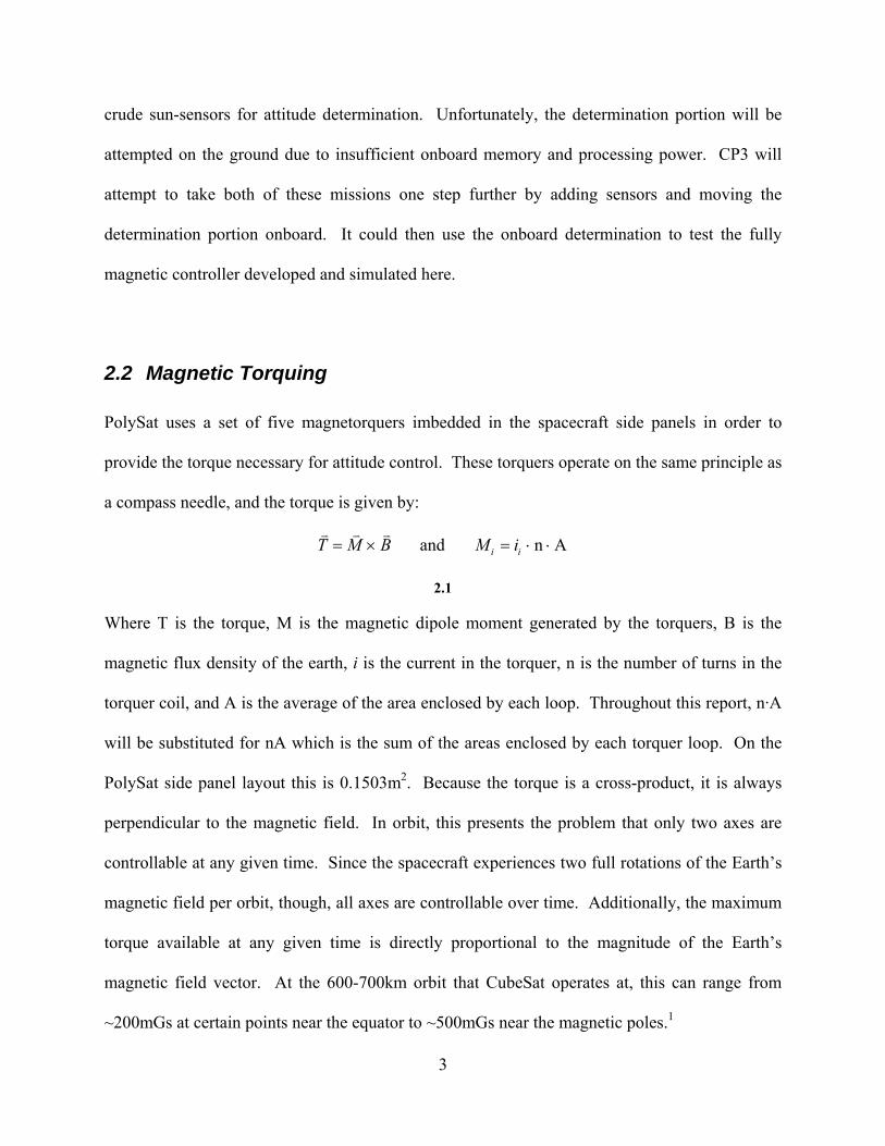
PolySat uses a set of five magnetorquers imbedded in the spacecraft side panels in order to
provide the torque necessary for attitude control. These torquers operate on the same principle as
a compass needle, and the torque is given by:
T M B= ×v v v
and n Ai iM i= ⋅ ⋅
2.1
Where T is the torque, M is the magnetic dipole moment generated by the torquers, B is the
magnetic flux density of the earth, i is the current in the torquer, n is the number of turns in the
torquer coil, and A is the average of the area enclosed by each loop. Throughout this report, n·A
will be substituted for nA which is the sum of the areas enclosed by each torquer loop. On the
PolySat side panel layout this is 0.1503m2. Because the torque is a cross-product, it is always
perpendicular to the magnetic field. In orbit, this presents the problem that only two axes are
controllable at any given time. Since the spacecraft experiences two full rotations of the Earth’s
magnetic field per orbit, though, all axes are controllable over time. Additionally, the maximum
torque available at any given time is directly proportional to the magnitude of the Earth’s
magnetic field vector. At the 600-700km orbit that CubeSat operates at, this can range from
~200mGs at certain points near the equator to ~500mGs near the magnetic poles.1
4
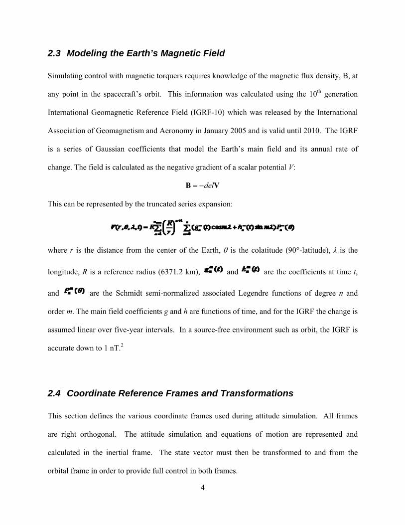
2.3 Modeling the Earth’s Magnetic Field
Simulating control with magnetic torquers requires knowledge of the magnetic flux density, B, at
any point in the spacecraft’s orbit. This information was calculated using the 10th generation
International Geomagnetic Reference Field (IGRF-10) which was released by the International
Association of Geomagnetism and Aeronomy in January 2005 and is valid until 2010. The IGRF
is a series of Gaussian coefficients that model the Earth’s main field and its annual rate of
change. The field is calculated as the negative gradient of a scalar potential V:
del= −B V
This can be represented by the truncated series expansion:
where r is the distance from the center of the Earth, θ is the colatitude (90°-latitude), λ is the
longitude, R is a reference radius (6371.2 km), and are the coefficients at time t,
and are the Schmidt semi-normalized associated Legendre functions of degree n and
order m. The main field coefficients g and h are functions of time, and for the IGRF the change is
assumed linear over five-year intervals. In a source-free environment such as orbit, the IGRF is
accurate down to 1 nT.2
2.4 Coordinate Reference Frames and Transformations
This section defines the various coordinate frames used during attitude simulation. All frames
are right orthogonal. The attitude simulation and equations of motion are represented and
calculated in the inertial frame. The state vector must then be transformed to and from the
orbital frame in order to provide full control in both frames.

5
2.4.1 The Body Frame
This frame has axes that correspond to the principle inertial axes of the spacecraft and an origin
at the spacecraft center of gravity. For simplicity, these are assumed to coincide with the
primary structural axes of the spacecraft.
2.4.2 The Inertial Frame
This frame has an origin at the center of gravity of the spacecraft and translates with the
spacecraft as it orbits. The i1 axis is parallel to a line drawn from the center of the Earth through
the spacecraft’s perigee. The i2 axis lies in the orbital plane and runs parallel to the spacecraft’s
velocity vector at perigee. The i3 axis is perpendicular to the orbital plane and follows the right
hand rule. Throughout this paper, angular rates given in the inertial frame refer to rates taken
along the body axes but represent motion relative to the inertial frame. Quaternions referenced
in the inertial frame represent the Euler-axis rotation from the inertial to body reference frames.
The simulation software developed for this report calculates all attitude differential equations in
this frame.
2.4.3 The Orbital Frame
This frame also has an origin at the center of gravity of the spacecraft and translates with the
spacecraft as it orbits. The o1 axis is collinear with a line drawn from the center of the Earth
through the spacecraft’s center of gravity, also known as the local vertical. The o2 axis lies in the
orbital plane and represents the local horizontal. The o3 axis is perpendicular to the orbital plane,
follows the right hand rule, and coincides with the i3 axis. The angle between the i1 and o1 and

6
also between the i2 and o2 axes is equal to ν, the true anomaly. Angular rates given in the orbital
frame refer to rates taken along the body axes but represent motion relative to the orbital frame.
Quaternions referenced in the orbital frame represent the Euler-axis rotation from the orbital to
body reference frames. Since the simulation itself does not use this frame, results given in the
orbital frame are shown for reference only. The following figure shows the relationship between
the orbital and inertial frames.
Figure 2.1: The inertial and orbital frames
2.4.4 Successive Quaternion Rotations
Since the simulation is run in inertial frame, the orbital quaternion vector represents two
successive quaternion rotations. The first is from the inertial to the orbital frame and the second
between the body and inertial frame. The composite rotation is given by the following equation:1
4 3 2 1 1123 4 1 2 22
22 1 4 3 33
1 2 3 4 44
D
D
D
D
q q q q qqq q q q qq
q q q q qqq q q q qq
′′ ′′ ′′ ′′ ′−⎡ ⎤ ⎡ ⎤ ⎡ ⎤⎢ ⎥ ⎢ ⎥ ⎢ ⎥′′ ′′ ′′ ′−⎢ ⎥ ⎢ ⎥ ⎢ ⎥=⎢ ⎥ ′′ ′′ ′′⎢ ⎥ ′⎢ ⎥−⎢ ⎥ ⎢ ⎥ ⎢ ⎥′′ ′′ ′′ ′′ ′− − − ⎢ ⎥⎢ ⎥⎢ ⎥ ⎣ ⎦⎣ ⎦⎣ ⎦
o2
i2, o2
i1, o1
i2
i1o1
o2
i2
i1
o1
ν
i3, o3 axes come out of
page

7
The transformation between inertial and orbital frames is a single rotation about the 3rd axis, so
the rotation quaternions are:
( ) ( )0 0 sin cos2 2T
ioν ν⎡ ⎤′ = =
⎣ ⎦q q and i′′ =q q
While the substitution for the reverse from and orbital to inertial quaternion is given by:
( ) ( )0 0 sin cos2 2T
oiν ν⎡ ⎤− −′ = =
⎣ ⎦q q and o′′ =q q
2.4.5 Transformation of Angular Rates
Since the rates are referenced to the body axis in both the orbital and inertial frames, this
transformation is actually just the subtraction or addition of the rotation rate between the orbital
and inertial frames. The rotation of the orbital frame relative to the inertial frame is equal to the
mean motion, or [ ]0 0 Toiω ν=v . Before this vector can be added or subtracted, however, it
must be transformed into the body frame by way of the transformation matrix.1
( ) ( ) ( )( ) ( ) ( )( ) ( ) ( )
2 22 3 1 2 3 4 1 3 2 4
2 21 2 3 4 1 3 2 3 1 4
2 21 3 2 4 2 3 1 4 1 2
1 2 2 2
2 1 2 2
2 2 1 2
i b
q q q q q q q q q q
q q q q q q q q q q
q q q q q q q q q q
⎡ ⎤− + + −⎢ ⎥⎢ ⎥= − − + +⎢ ⎥⎢ ⎥+ − − +⎣ ⎦
T
2.2
Where the inertial quaternion vector is used. The full equations for the transformations of the
angular rates are given by:
o i i b oiω ω ω= − ⋅Tv v v and i o i b oiω ω ω= + ⋅Tv v v

8
2.5 The Equations of Motion
The Euler equations of motion for the angular velocities of a spinning, rigid-body spacecraft are:
2 3 11 2 3
1 1
3 1 22 1 3
2 2
31 23 1 2
3 3
I I TI I
I I TI I
TI II I
ω ω ω
ω ω ω
ω ω ω
⎛ ⎞−= +⎜ ⎟⎝ ⎠⎛ ⎞−
= +⎜ ⎟⎝ ⎠⎛ ⎞−
= +⎜ ⎟⎝ ⎠
&
&
&
Where T represents the torques acting on the spacecraft, which can be either internal (control) or
external (disturbance). The angular position of the spacecraft is represented in quaternions, and
their governing differential equation is:
3 2 11 1
3 1 22 2
2 1 33 3
1 2 34 4
00
00
q qq qq qq q
ω ω ωω ω ωω ω ωω ω ω
−⎡ ⎤⎡ ⎤ ⎡ ⎤⎢ ⎥⎢ ⎥ ⎢ ⎥−⎢ ⎥⎢ ⎥ ⎢ ⎥=⎢ ⎥⎢ ⎥ ⎢ ⎥−⎢ ⎥⎢ ⎥ ⎢ ⎥− − −⎢ ⎥ ⎢ ⎥⎢ ⎥⎣ ⎦ ⎣ ⎦⎣ ⎦
&
&
&
&
Together with a numerical differential equation solver, these seven equations allow the
propagation of the spacecraft attitude for any time. They return the state vector in the inertial
reference frame.
2.6 Attitude Disturbance Torques
The four main disturbance torques that would affect a picosatellite in LEO are magnetic,
aerodynamic, gravity gradient and solar pressure in order of magnitude. The following equations
were taken from Space Mission Analysis and Design (SMAD).3 The numbers shown are for 600
km orbit, which is the low side of what a CubeSat program will see. Therefore, these
disturbances are worst-case.
9
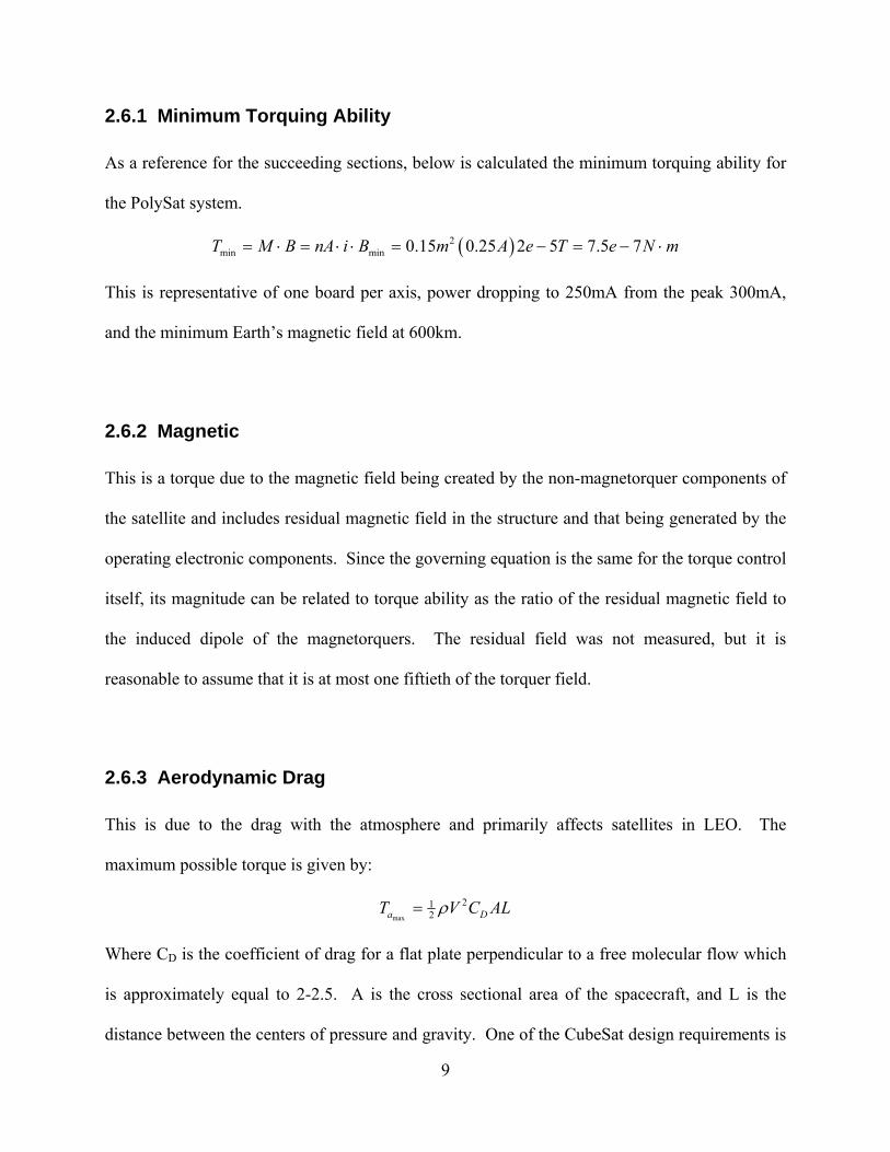
2.6.1 Minimum Torquing Ability
As a reference for the succeeding sections, below is calculated the minimum torquing ability for
the PolySat system.
( )2min min 0.15 0.25 2 5 7.5 7T M B nA i B m A e T e N m= ⋅ = ⋅ ⋅ = − = − ⋅
This is representative of one board per axis, power dropping to 250mA from the peak 300mA,
and the minimum Earth’s magnetic field at 600km.
2.6.2 Magnetic
This is a torque due to the magnetic field being created by the non-magnetorquer components of
the satellite and includes residual magnetic field in the structure and that being generated by the
operating electronic components. Since the governing equation is the same for the torque control
itself, its magnitude can be related to torque ability as the ratio of the residual magnetic field to
the induced dipole of the magnetorquers. The residual field was not measured, but it is
reasonable to assume that it is at most one fiftieth of the torquer field.
2.6.3 Aerodynamic Drag
This is due to the drag with the atmosphere and primarily affects satellites in LEO. The
maximum possible torque is given by:
max
212a DT V C ALρ=
Where CD is the coefficient of drag for a flat plate perpendicular to a free molecular flow which
is approximately equal to 2-2.5. A is the cross sectional area of the spacecraft, and L is the
distance between the centers of pressure and gravity. One of the CubeSat design requirements is

10
that the spacecraft c.g. be within 2 cm of the geometric center of the spacecraft. This number
will be used here even though the actual c.g. of CP2 was considerably within this limit. Plugging
in the numbers for a 600km orbit yields:
( )( ) ( )3max
2 212 4.89 13 7550 2.5 0.01 0.02 6.97 9kg m
a smT e m m e N m= − = − ⋅
2.6.4 Gravity Gradient
This is due to the difference in the pull of gravity across the spacecraft. The maximum gravity
gradient (GG) torque is given by:
( )max
2max min max3ggT I I n= −
Where Imax and Imin are the maximum and minimum principle moments of inertia and n is the
orbital angular velocity of the spacecraft. Most CubeSats will be inserted into nearly circular
orbits, so this term can be substituted for the mean motion.
( ) ( )max
220.0005 3 0.00108 1.75 9radgg sT kg m e N m= ⋅ = − ⋅
Where the mean motion for a 600km circular orbit is used. The difference in principle inertias is
estimated based on the value from the CP2 solid model (0.0002kg·m2) and a factor of safety of
2.5.
2.6.5 Solar Pressure
This is a torque due to impact with solar wind. Like aerodynamic drag, it is mainly a function of
the distance between the centers of pressure and gravity. The maximum torque is given by:
max(1 )s
spF
T A r Lc
= +
11
Where Fs is solar flux (1367 W/m2), c is the speed of light (3e8 m/s), and r is the solar
reflectance factor. Even substituting the improbably high reflectance factor of 0.8, the maximum
possible torque is only:
2
max
21367
0.01 (1 0.8)0.02 1.64 93 8
Wm
sp ms
T m m e N me
= + = − ⋅
2.6.6 Summary
The following table compares the results of the previous sections.
Table 2.1: Worst Case Attitude Disturbance Torques
Torque Type N*m Minimum Torquing Ability 7.50e-07Residual S/C Magnetic Field 2.00e-08Aerodynamic 6.97e-09Gravity Gradient 1.75e-09Solar Pressure 1.64e-09
Since these torques are all roughly two orders of magnitude smaller than even the minimum
torquing ability, all but gravity gradient were not modeled in the attitude simulation.
2.7 Survey of the Field
While the use of magnetic torquing is nothing new to the satellite community, no program has
yet even attempted to fly a nano- or picosatellite using solely magnetic control. Below are
summarized several reports and papers that were useful in designing this system.
12
2.7.1 B-dot Controller
For his thesis, Kristian Svartveit of Norway’s NCUBE program summarized the development
and testing of their Attitude determination system.4 As a member of the CubeSat program,
NCUBE was subject to the same size and mass restriction as PolySat. Their control system
consisted of both magnetorquers and a small boom for gravity gradient (GG) stabilization. A
pointing accuracy of 10º-20º was necessary in order to use the broadband antenna they had
onboard. Their system used two different magnetic control algorithms but relied entirely on the
GG boom for their pointing accuracy. The first magnetic algorithm was the B-dot detumbling
controller and the second would simply tip the spacecraft 90º in case it accidentally aligned with
the GG boom pointed away from Earth. Their attitude determination system used a Kalman
filter to reduce noise and integrate attitude information from a set of magnetometers and crude,
solar panel sun sensors. While the analysis was not particularly helpful due to the addition of the
GG boom, it did contain pseudo-code for B-dot which was useful for designing the algorithm
used here. There was no on-orbit data in this report because it was written before the launch of
the satellite.
Another CubeSat program to use B-dot was the AAU CubeSat by Aalborg University in
Denmark.5 This team also developed constant-gain and LMI controllers for three-axis pointing
stability. All of the analysis was done for periodic linear systems, however, which are not a very
accurate representation of the mechanics involved. Unfortunately, contact was never made with
this satellite after deployment, so no on-orbit information is available.

13
2.7.2 Three-Axis Controller
Several theoretical studies were found that talked about the possibility of three-axis stabilization.
They were not particularly useful due to their use of supplementary non-magnetic actuators or
linear analysis. The most useful information for the three-axis controller came from a report by
M. Guelman about the magnetic control experiments performed on the Israeli Guerwin-Techsat.6
This satellite was a 50kg cube, was launched in July 1998, and successfully functioned for over
4.5 years. They had both magnetorquers and a momentum wheel onboard which was shut down
for several on-orbit, full magnetic control tests. Three magnetic controllers were developed for
three-axis stabilization, called the COMPASS, linear quadratic regulator (LQR), and No-Wheel
controllers. The COMPASS controller used the law:
( ) ( )1 2measured expected measured expectedm C B B C B B= − − − −v v v vv & &
The No-Wheel controller, named for the complete shutdown of the momentum wheel, followed
the law:
( )11 2req e eT C C I qω −= − ⋅ + ⋅ ⋅
v v v
The LQR controller was not used because of its linear approximations. The COMPASS
controller was tested for the PolySat system, but was found to be less accurate than a No-Wheel-
type controller. This report also presented the pseudo-reverse of the cross-product from equation
2.1 that is presented later. Their tests showed that with even a very small momentum bias
accuracies of 2º-2.5º were possible. Regrettably, due to a malfunction of the linear Kalman filter
and the fact that the momentum wheel was not equipped with a break, they were not able to
achieve fully magnetic three-axis stabilization.

14
3 HARDWARE
The PolySat team has designed and is refining a standardized bus that will be used on future
incarnations and could be sold to or shared with other schools and companies. This bus consists
of several standardized components: an aluminum structure, the CD&H board, the power board,
four side panels, and a front panel (left-most face, Figure 3.1 below). The remaining face is left
for a payload-specific board and there is an internal mount for another payload board.
Figure 3.1: CP2 Engineering Model

15
3.1 Side and Front Panels
The side panels each have two solar panels, a magnetometer, magnetorquer coils, two
temperature sensors, and the electronics to control all these devices. The front panel has the
same equipment as the side panels with the addition of the antenna route, antenna, and holes for
the remove-before-flight pin and diagnostic port. The standard configuration is for four side
panels and one front panel. The sixth face could be equipped with another side panel or reserved
for the payload, as is the case with CP2 and CP3.
Figure 3.2: CP2 side panel interior face
16
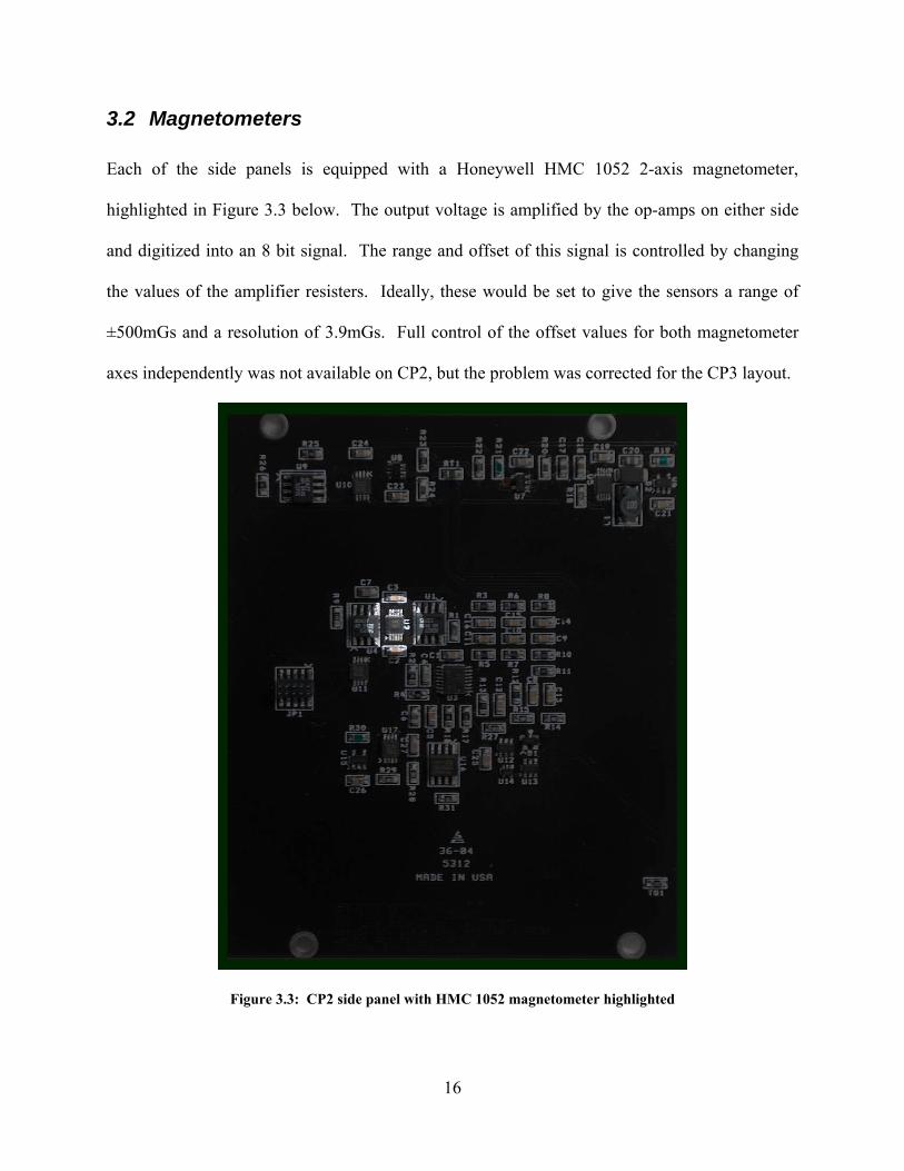
3.2 Magnetometers
Each of the side panels is equipped with a Honeywell HMC 1052 2-axis magnetometer,
highlighted in Figure 3.3 below. The output voltage is amplified by the op-amps on either side
and digitized into an 8 bit signal. The range and offset of this signal is controlled by changing
the values of the amplifier resisters. Ideally, these would be set to give the sensors a range of
±500mGs and a resolution of 3.9mGs. Full control of the offset values for both magnetometer
axes independently was not available on CP2, but the problem was corrected for the CP3 layout.
Figure 3.3: CP2 side panel with HMC 1052 magnetometer highlighted

17
3.3 Magnetorquers
Each side panel contains a sandwich of three layers with 18 coils each for a total of 54 turns and
a total enclosed area of 0.1503m2. Figure 3.4 below has the approximate coil location
superimposed over the panel. Note that the number of coils shown below is not correct. Current
is controlled by a pulse-width modulator to provide a current of at most ±300mA. The
maximum value will change depending on battery charge and power available. The current is
controlled by two commands of one byte. One is for the direction and the other is the magnitude.
This gives the magnetorquer current a resolution of 1.2 mA.
Figure 3.4: CP2 Side Panel with approximate torquer location

18
4 ATTITUDE SIMULATION COMPONENTS
The attitude simulation is based on a tool developed by fellow graduate student Erick Sturm
called the Orbit Propagator and Attitude Simulator (OPAS). The attitude portion of this
simulation was highly modified in order to implement and debug full 3-axis control of a
simulated PolySat. The inertial properties of the spacecraft were taken from the IDEAS model
of CP2, however, different sizes of satellite may be simulated using this tool by changing the
inertias and gains appropriately. The code is reprinted in Appendix C in its entirety.
4.1 Orbit Propagator
This portion of OPAS was left largely in its original form and includes the J2, third body, and
atmospheric drag disturbance terms. Results are displayed in the form of a ground track. It also
calculates the magnetic field at every time step of the propagation. This information is then
interpolated for every point in the attitude simulation.
4.2 Magnetic Field Estimation
The magnetic field at every point in the simulation was calculated by a MATLAB program
called “magfd” developed by Maurice Tivey at the Woods Hole Marine Magnetism Group.7
This program accepts the spacecraft location in space and time and returns the magnetic field
vector as estimated by the IGRF-10 Gaussian coefficients. Field information is calculated at
each step of the orbit propagation, and linearly interpolated for intermediate points of the attitude
simulation. The “magfd” code is reprinted in Appendix A.

19
4.3 Disturbance Torques
The only disturbance torque modeled in this attitude simulation was that of gravity gradient
simply because it is very easy to implement. The Euler equations are modified in this fashion:
22 3 2 311 2 3 21 31
1 1 1
23 1 3 122 1 3 11 31
2 2 2
231 2 1 23 1 2 11 21
3 3 3
3
3
3
I I I ITn C C
I I I
I I I ITn C C
I I I
TI I I In C C
I I I
ω ω ω
ω ω ω
ω ω ω
⎛ ⎞ ⎛ ⎞− −= + −⎜ ⎟ ⎜ ⎟⎝ ⎠ ⎝ ⎠⎛ ⎞ ⎛ ⎞− −
= + −⎜ ⎟ ⎜ ⎟⎝ ⎠ ⎝ ⎠⎛ ⎞ ⎛ ⎞− −
= + −⎜ ⎟ ⎜ ⎟⎝ ⎠ ⎝ ⎠
&
&
&
Where the Cii terms come from the body-to-inertial quaternion transformation matrix of equation
2.2. Including it in the simulation had a negligible affect on the results. Its magnitude is
compared with other possible disturbances in Table 2.1. Even though other disturbances are not
simulated, they are of similar magnitude to gravity gradient. Since there was a negligible
difference between the results with and without GG, it is probable that the other disturbances
would have little effect as well.
4.4 Hardware Models
Each of the components of the ADCS introduces another level of uncertainty to the system. This
is represented here by adding a normally-distributed random noise component and rounding each
value to the component’s resolution.
4.4.1 Magnetorquers
The magnetorquers were first simulated by assigning each component of the magnetic dipole
requested to one torquer panel. These requests were converted to a current command by

20
equation 2.1. The current command was then limited so that no individual magnetorquer would
request more than the hardware limit of 300mA. The current was limited by halving all
components until they were within the maximum allowed. This method was chosen based on the
advice of the software team due to the fact that a division by two is a simple bit flip in binary
math. Finally, a two byte command is sent to the pulse-width modulator (PWM) that controls
the torquer current. The first byte gives the current direction while the second breaks the full
range from 0-300mA into 256 steps, so the current requested by the simulation was rounded off
to the nearest 1.2 mA.
4.4.2 Magnetometers
The magnetometers were modeled in several different ways to test varying degrees of accuracy
and methods of implementation. In the actual hardware, the voltage from the actual
magnetometers is converted into a one bit number for each of the two axes that it reports. The
relationship between this voltage and magnetic flux density is linear and given by the equation:
(bit value)M a b= +
4.1
Where a and b are calibration factors. With five side panels and two axes each, there are ten
channels of information. This provides double redundancy on two axes and triple redundancy on
the third. The reading of each of the ten magnetometers is simulated using:
( )( )/ *ij i mtmt round B b a randnσ= − +
4.2
Where mtij is the jth reading of body axis i and is given in bits. Round is a function that rounds
the reading to the nearest bit value. The last term adds a noise where σ is the standard deviation

21
of the noise and randn is a function that returns a random number with mean zero and a standard
deviation of one. In other words, this simulates a reading with the correct resolution of the
magnetometers and introduces a noise with standard deviation of σ. Two different versions of
the calibration factors were simulated.
4.4.2.1 Ideal Calibration
In this case, it is assumed that the resistors controlling each channel of the magnetometers are
appropriately sized so that each channel reports a 0 at -500 mGs and 255 at 500 mGs, which is
slightly above the 480mGs that will be seen on orbit1. With 256 steps between ±500 mGs, this
gives the magnetometers a resolution of approximately 4 mGs. The bit value is converted back
to magnetic flux density using equation 4.1 and plugging in a = 5e-5/128 T/bit and b = -5e-5 T.
The median is then taken of the three or four readings for each axis. This is done so that
readings from any malfunctioning magnetometers on orbit would be discarded. This three-
component vector is then returned to the simulation and used for the calculation of magnetorquer
commands.
4.4.2.2 Real CP2 Calibration Information with B-dot Bit Calculation
This case simulates the actual way in which CP2 will calculate and execute B-dot. It differs
from the previous one in that the a and b calibration values are taken from the actual test data for
the CP2 flight side boards. The calibration data are given in Appendix B and were taken in a
very rough manner not intended for attitude extrapolation. Since these data are not stored
onboard CP2, this method also differs in that the bit values are not converted back into magnetic

22
flux values. Accuracy is decreased because each magnetometer has a different range and offset
which could conflict with each other. As before, the median is then taken of the three or four
readings for each axis. The goal of this version is to demonstrate that readings from
magnetometers with different zero points, ranges, and resolutions can still be combined for
effective control.
4.4.3 Other Possible Attitude Determination Hardware
In order for the three-axis control algorithm to function, full knowledge of the spacecraft position
and rates is required. Several methods are under consideration for the CP3 project including an
extended Kalman filter for the magnetometer data, gyros, star trackers, and sun sensors. These
would be mounted on the payload board or payload face. In order to maintain generality and
since the final architecture had not yet been decided at the time of writing, the simulated
quaternions and rates were modified with an arbitrary noise and resolution as shown below.
( ),exacti iround randnωω ω σ δω= + ⋅
( ),exacti i qq round q randn qσ δ= + ⋅
4.3
Where the σ’s are the standard deviation of the noise and the round function rounds the reading
off to the nearest step of the resolution, δω or δq. Rather than plug in given values, this report
will examine what noise levels and resolutions are required for convergence of the three-axis
algorithm.

23
4.5 B-dot Detumbling Algorithm
The calculation of B-dot itself was done by a simple backwards difference method:
t t t
t
δ
δ
−−=
B BB)& req K= − ⋅M B
)&
4.4
Where the gain was found through trial-and-error by decreasing its value until the system the
fastest settling time was reached. As described in Section 4.4.2.2, on CP2 the values for B and
B-dot are calculated as unitless bit values, whereas the preferable method is to convert each
magnetometer reading into tesla prior to calculation of B-dot. As written for CP2, the inputs for
the B-dot command are the total run time, gain, time between readings, wait time, and torquer
pulse time.
4.6 Three-Axis Control Algorithm
The more complicated of the control algorithms, full control in three axes requires accurate
attitude knowledge to function correctly. The algorithm itself is just a simple rate and position
feedback similar to the one used on the Gurwin-Techsat5:
( )1 2req e eT C C qω= − ⋅ + ⋅Iv v v
Where Treq is the requested torque, C1 and C2 are gains, and ωe is the error in angular velocity.
The equation is multiplied by I, the principle moment of inertia vector, in order to size each
torque appropriately to the axis about which it is torquing. Rather than the entire quaternion, the
vector qe is the first three components of the quaternion error vector, which approximate the
Euler angles for small angles. The entire vector is given by the equation:8

24
4 3 2 1 1
3 4 1 2 2
2 1 4 3 3
1 2 3 4 4
d d d d a
d d d d a
d d d d a
d d d d a
q q q q qq q q q q
q q q q qq q q q q
− −⎡ ⎤ ⎡ ⎤⎢ ⎥ ⎢ ⎥− −⎢ ⎥ ⎢ ⎥=⎢ ⎥ ⎢ ⎥− −⎢ ⎥ ⎢ ⎥⎢ ⎥ ⎢ ⎥⎣ ⎦ ⎣ ⎦
eq
4.5
Where qd is the desired vector and qa is the actual quaternion. When the desired vector was
given in the orbital frame, it was converted to the inertial frame at each time step and then input
into the quaternion error equation above. Since the frames are rotating relative to each other, this
meant that the desired quaternions would oscillate as the system settled out to a constant rotation
in the inertial frame. Refer back to sections 2.4 for this transformation procedure.
The next step is to convert the desired torque vector into a magnetorquer command. As
mentioned in Section 2.2, the torque cannot be commanded directly since the possible torque
vector is always perpendicular to the magnetic field. Instead, the magnetic dipole is requested
using5:
2req
req
B TM
B
×=
v vv
v
4.6
This equation saves power by only torquing the portion of the requested vector perpendicular to
the magnetic field and is a best-fit approximation of the reverse of the cross-product from
equation 2.1.
25
4.7 Computation
The flow of the attitude simulation portion was written in order to mimic the computational flow
onboard the actual satellite as much as possible. The main controller parameters are those of the
gains (K for B-dot and C1 and C2 for three-axis) and the pulse length, δt. The pulse length
defines both the time between magnetometer readings and the time that the torquers are pulsed
for before the cycle is repeated. A complete controller cycle consists of:
st
nd
1 reading Wait t
2 reading Wait 0.1 sec for torque command calculation
Turn on torquers Wait t
Turn off torquers Wait 0.1 sec for torque field to die out
δ
δ
→ →
→ →
→ →
→
The 0.1 seconds after the second magnetometer reading was set in order to simulate the time it
might take the processor to handle the attitude information and calculate the necessary current
commands. The 0.1 sec after torquing was determined from experimental data for the
magnetometer readings. It was found that magnetometer readings taken immediately after
pulsing the torquers were greatly skewed by the residual magnetic field, but even a small buffer
such as this was sufficient to allow the induced field to dissipate.

26
4.8 Summary of Simulation Assumptions
While an attempt was made to make the simulation as real as possible, a point of diminishing
returns must be considered when eliminating assumptions. Consequently, several
approximations were kept in the simulation. They are:
• The spacecraft is a rigid body.
• The principal inertial and structural axes coincide.
• Disturbance torques other than gravity-gradient are negligible.
• The power subsystem is always capable of providing 300mA per torquer.
• There is a properly functioning attitude determination system in operation.
• Sensors are properly calibrated and mounted, i.e. there is no misalignment or offset error.
• Command computation needs can be met in 0.1 seconds.
27
5 ATTITUDE SIMULATION RESULTS
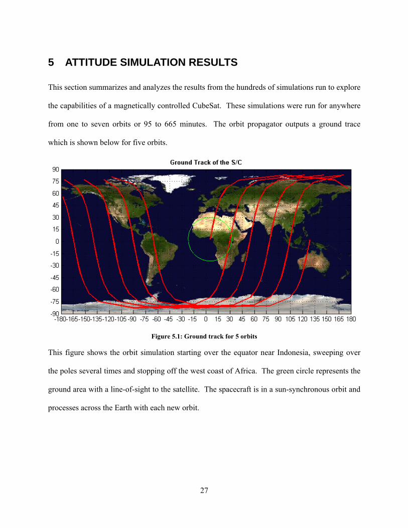
This section summarizes and analyzes the results from the hundreds of simulations run to explore
the capabilities of a magnetically controlled CubeSat. These simulations were run for anywhere
from one to seven orbits or 95 to 665 minutes. The orbit propagator outputs a ground trace
which is shown below for five orbits.
Figure 5.1: Ground track for 5 orbits
This figure shows the orbit simulation starting over the equator near Indonesia, sweeping over
the poles several times and stopping off the west coast of Africa. The green circle represents the
ground area with a line-of-sight to the satellite. The spacecraft is in a sun-synchronous orbit and
processes across the Earth with each new orbit.

28
5.1 B-dot Detumbling
Many simulations were run in order to optimize the two main control parameters, the gain from
equation 4.4 and the pulse length. After these were found, many more simulations were run to
analyze the system’s performance under less than ideal conditions. The failure modes that were
analyzed were those of high tip-off velocities, noisy magnetometer readings, and torquer failure.
Additionally, the B-dot calculation methods of CP2 and CP3 were compared.
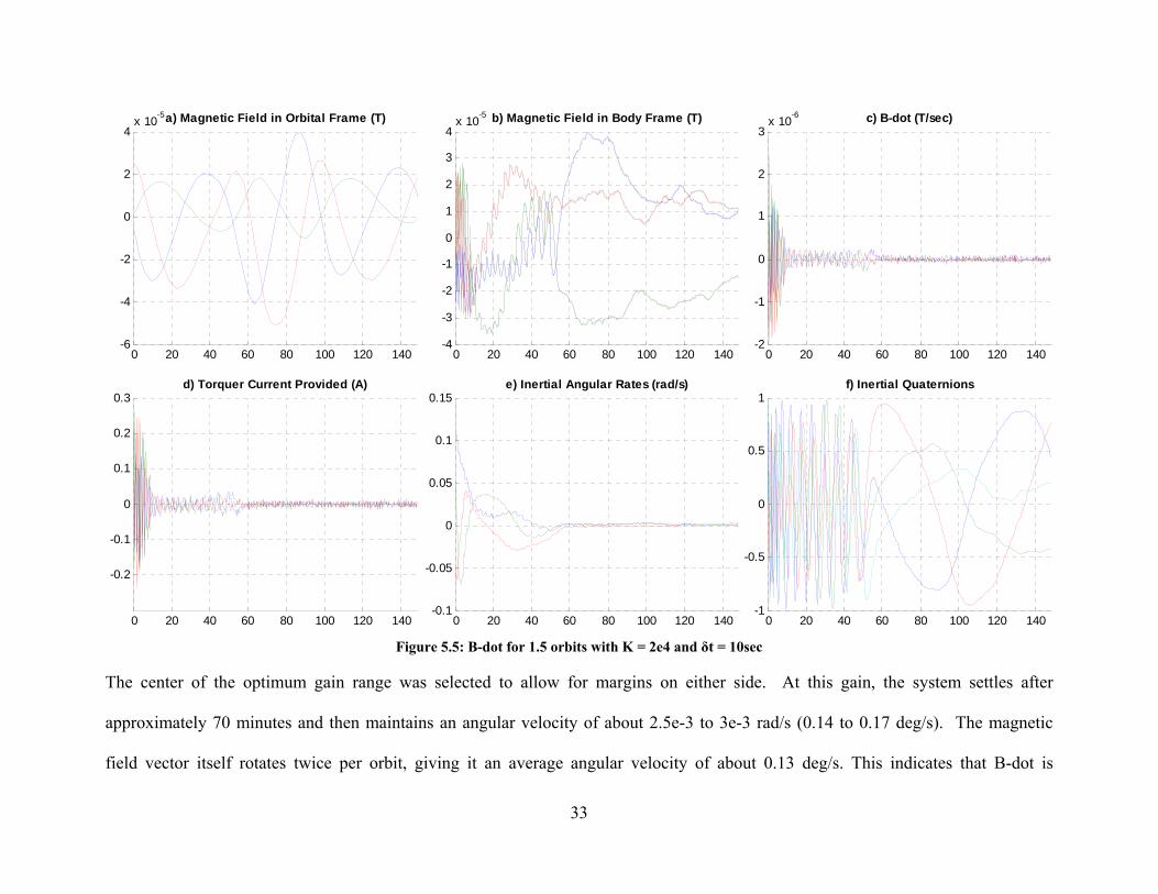
5.1.1 Explanation of B-dot plots
The results of each simulation are summarized in a single figure divided into six subplots which
are lettered from a-f. The x-axis of all plots is given in minutes. One may use the orbital period
of approximately 95 minutes to convert these values to fractions of an orbit. With the exception
of the quaternions, the lines within each subplot represent Cartesian axes and are colored
according to:
Axis 1: Blue
Axis 2: Green
Axis 3: Red
Axis 4: Cyan (for the fourth quaternion or magnitude of the angular velocity only)
An explanation of each subplot follows:
a) Magnetic Field in the Orbital Frame displays the components of the magnetic field found
in the orbit propagator by magfd (see Section 4.2).
b) Magnetic Field in the Body Frame shows the magnetic field components seen by the
sensors. The gray lines represent the values measured by the spacecraft and include any
noise terms.

29
c) B-dot shows the values calculated by the B-dot algorithm.
d) Torquer Current Provided relates to B-dot by a factor of K/nA but is also bound by the
current limiter described in Section 4.4.1.
e) Inertial Angular Rates are the actual simulated values. These are given as a reference
and not used in the control algorithm. See Section 2.4.2 for a definition of the frame.
f) Inertial Quaternions are the actual simulated values shown for reference.
5.1.2 Optimum Gain Determination
The optimum gain was found by simulating a range of values and selecting the one that settled
the fastest. These simulations were run for 1½ orbits and had minimal noise in the
magnetometer readings. The initial angular velocities were set at ω = [0.1 -0.05 0.05]T which is
approximately 1 rpm about the b1 axis. The pulse lengths were set to ten seconds. There were
three types of unstable behavior: complete instability, instability starting at the North Pole, and
instability localized to the North Pole. These distinctions were due to the fact that the effective
gain changes with the fluctuation of the local magnetic field, which is the strongest at the North
Pole. The first—complete instability—occurred for gains of about 1.7e5 and higher. Figure 5.2
below shows the results of this simulation.

30
0 20 40 60 80 100 120 140-6
-4
-2
0
2
4x 10⁻⁵a) Magnetic Field in Orbital Frame (T)
0 20 40 60 80 100 120 140-6
-4
-2
0
2
4
6x 10⁻⁵ b) Magnetic Field in Body Frame (T)
0 20 40 60 80 100 120 140-1
-0.5
0
0.5
1x 10⁻⁵ c) B-dot (T/sec)
0 20 40 60 80 100 120 140
-0.2
-0.1
0
0.1
0.2
0.3d) Torquer Current Provided (A)
0 20 40 60 80 100 120 140-0.8
-0.6
-0.4
-0.2
0
0.2
0.4
0.6
0.8e) Inertial Angular Rates (rad/s)
0 20 40 60 80 100 120 140-1
-0.5
0
0.5
1f) Inertial Quaternions
Figure 5.2: B-dot for 1.5 orbits with K = 17e4 and δt = 10sec
Plot d) shows that the gain is so high that magnetorquer current is being clipped for the entire simulation. Even so, B-dot reduces the
angular velocities initially, but then some disturbance sends it spinning about the major inertial axis, b3. The additional instability
around 70 minutes corresponds to a peak in the magnetic field as shown in plot a). This peak occurs as the satellite transits the North
Pole and is further examined in the following simulation.

31
0 20 40 60 80 100 120 140-6
-4
-2
0
2
4x 10⁻⁵a) Magnetic Field in Orbital Frame (T)
0 20 40 60 80 100 120 140-6
-4
-2
0
2
4
6x 10⁻⁵ b) Magnetic Field in Body Frame (T)
0 20 40 60 80 100 120 140-1
-0.5
0
0.5
1x 10⁻⁵ c) B-dot (T/sec)
0 20 40 60 80 100 120 140
-0.2
-0.1
0
0.1
0.2
0.3d) Torquer Current Provided (A)
0 20 40 60 80 100 120 140-0.8
-0.6
-0.4
-0.2
0
0.2
0.4
0.6e) Inertial Angular Rates (rad/s)
0 20 40 60 80 100 120 140-1
-0.5
0
0.5
1f) Inertial Quaternions
Figure 5.3: B-dot for 1.5 orbits with K = 11e4 and δt = 10sec
The second instability case occurs for gains between approximately 1.1e5 and 1.7e5. The satellite initially settles but then diverges as
near the pole. Not only is the field strength highest here, but also its rate of change of direction. At this point the torquers have
become saturated and the angular velocities too great for the system to recover. Again, the spacecraft spins about the major axis.

32
0 20 40 60 80 100 120 140-6
-4
-2
0
2
4x 10⁻⁵a) Magnetic Field in Orbital Frame (T)
0 20 40 60 80 100 120 140-6
-4
-2
0
2
4
6x 10⁻⁵ b) Magnetic Field in Body Frame (T)
0 20 40 60 80 100 120 140-6
-4
-2
0
2
4
6x 10⁻⁶ c) B-dot (T/sec)
0 20 40 60 80 100 120 140
-0.2
-0.1
0
0.1
0.2
0.3d) Torquer Current Provided (A)
0 20 40 60 80 100 120 140-0.1
-0.05
0
0.05
0.1
0.15e) Inertial Angular Rates (rad/s)
0 20 40 60 80 100 120 140-1
-0.5
0
0.5
1f) Inertial Quaternions
Figure 5.4: B-dot for 1.5 orbits with K = 8e4 and δt = 10sec
In this case the rates only explode near the pole, but do not diverge enough that the system cannot recover. Gains lower than about
7e4 converged at all points in the orbit; however, it was found that the maximum stable gain did not converge the fastest. The
optimum gains were found to be between 2.5e4 and 1.5e4. Figure 5.5 below shows the results for a gain of 2e4.
33
0 20 40 60 80 100 120 140-6
-4
-2
0
2
4x 10⁻⁵a) Magnetic Field in Orbital Frame (T)
0 20 40 60 80 100 120 140-4
-3
-2
-1
0
1
2
3
4x 10⁻⁵ b) Magnetic Field in Body Frame (T)
0 20 40 60 80 100 120 140-2
-1
0
1
2
3x 10⁻⁶ c) B-dot (T/sec)
0 20 40 60 80 100 120 140
-0.2
-0.1
0
0.1
0.2
0.3d) Torquer Current Provided (A)
0 20 40 60 80 100 120 140-0.1
-0.05
0
0.05
0.1
0.15e) Inertial Angular Rates (rad/s)
0 20 40 60 80 100 120 140-1
-0.5
0
0.5
1f) Inertial Quaternions
Figure 5.5: B-dot for 1.5 orbits with K = 2e4 and δt = 10sec
The center of the optimum gain range was selected to allow for margins on either side. At this gain, the system settles after
approximately 70 minutes and then maintains an angular velocity of about 2.5e-3 to 3e-3 rad/s (0.14 to 0.17 deg/s). The magnetic
field vector itself rotates twice per orbit, giving it an average angular velocity of about 0.13 deg/s. This indicates that B-dot is

34
performing very near the limit of its capability at this gain value. It was found that modifying
the other controller parameters had very little effect on the optimum gain setting, so a gain of 2e4
was used for the remainder of these experiments.
It is important to note that these gain values are highly dependent on the mass moment of inertia
of the spacecraft and should be recalculated for different configurations. The only consequence
of having the gain set too low is a proportional increase the settling time. Additionally, it was
found that stability can be improved for higher gains by decreasing the pulse time. The gain with
the fastest settling time, however, was well within this stability limit, so that is not a valid reason
to decrease pulse time. The relationship between pulse time and the maximum stable tip off
velocity is the subject of the next section.

35
5.1.3 Optimum Pulse Time Determination
While the gain is more directly related to the speed with which the system settles, the maximum
rotational velocity from which B-dot can recover is directly related to pulse length. B-dot
essentially assumes that the rate of change of the magnetic field does not change between the
field reading interval and the pulsing interval. As the actual rotation of the spacecraft increases,
this assumption becomes less valid until the nonlinearity makes the system unstable. This
problem is easily solved by decreasing the interval time, δt, so that the assumption is once again
valid. On the other hand, a larger interval time means less demand on the spacecraft’s processor
time, so these two design constraints must be traded.
For this investigation, the tip-off velocity was increased in 1 rpm increments and then the pulse
length shortened until the system converged. Now that the optimum gain has been found, all of
these simulations could be shortened to one orbit. The initial rates were [x -0.05 0.05] rad/s
where x is the test, tip-off velocity about the b1 axis and the other two represent perturbation
velocities. CubeSat’s investigations into its P-POD deployment system indicate that the most
probable maximum deployment rotation would be no greater than 1 rpm, so this was the first
point investigated.

36
0 20 40 60 80-6
-4
-2
0
2
4x 10⁻⁵a) Magnetic Field in Orbital Frame (T)
0 20 40 60 80-6
-4
-2
0
2
4x 10⁻⁵ b) Magnetic Field in Body Frame (T)
0 20 40 60 80-4
-3
-2
-1
0
1
2
3
4x 10⁻⁶ c) B-dot (T/sec)
0 20 40 60 80
-0.2
-0.1
0
0.1
0.2
0.3d) Torquer Current Provided (A)
0 20 40 60 80-0.1
-0.05
0
0.05
0.1
0.15e) Inertial Angular Rates (rad/s)
0 20 40 60 80-1
-0.5
0
0.5
1f) Inertial Quaternions
Figure 5.6: B-dot for 1 orbit with δt = 12 sec and ωo = 1 rpm
Given an initial velocity of 1 rpm, the largest interval for which the rates settle was found to be 12 seconds and the results are shown
above. As before in Figure 5.5 the rates settle within about 70 minutes, so this illustrates that δt has little effect on settling time.
Several more simulations were run at increasing velocities until a δt of one second was no longer sufficient to settle.

37
0 20 40 60 80 100 120 140-6
-4
-2
0
2
4x 10⁻⁵a) Magnetic Field in Orbital Frame (T)
0 20 40 60 80 100 120 140-6
-4
-2
0
2
4
6x 10⁻⁵ b) Magnetic Field in Body Frame (T)
0 20 40 60 80 100 120 140-6
-4
-2
0
2
4
6x 10⁻⁵ c) B-dot (T/sec)
0 20 40 60 80 100 120 140
-0.2
-0.1
0
0.1
0.2
0.3d) Torquer Current Provided (A)
0 20 40 60 80 100 120 140-0.5
0
0.5
1
1.5e) Inertial Angular Rates (rad/s)
0 20 40 60 80 100 120 140-1
-0.5
0
0.5
1f) Inertial Quaternions
Figure 5.7: B-dot for 1.5 orbit with δt = 1sec and ωo = 14 rpm
It was found that if the calculations could be done once every second, B-dot is capable of handling tip-off velocities of as high as 14
rpm. That is one revolution every 4.3 seconds, which is way beyond anything that the satellite would ever see. There was an increase
in settling time to the fact that the torquers are saturated while the angular velocity is above approximately 0.2 rad/s.
38
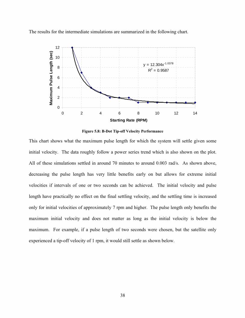
The results for the intermediate simulations are summarized in the following chart.
y = 12.304x-1.0378
R2 = 0.9587
0
2
4
6
8
10
12
0 2 4 6 8 10 12 14
Starting Rate (RPM)
Max
imum
Pul
se L
engt
h (s
ec)
Figure 5.8: B-Dot Tip-off Velocity Performance
This chart shows what the maximum pulse length for which the system will settle given some
initial velocity. The data roughly follow a power series trend which is also shown on the plot.
All of these simulations settled in around 70 minutes to around 0.003 rad/s. As shown above,
decreasing the pulse length has very little benefits early on but allows for extreme initial
velocities if intervals of one or two seconds can be achieved. The initial velocity and pulse
length have practically no effect on the final settling velocity, and the settling time is increased
only for initial velocities of approximately 7 rpm and higher. The pulse length only benefits the
maximum initial velocity and does not matter as long as the initial velocity is below the
maximum. For example, if a pulse length of two seconds were chosen, but the satellite only
experienced a tip-off velocity of 1 rpm, it would still settle as shown below.

39
0 20 40 60 80-6
-4
-2
0
2
4x 10⁻⁵a) Magnetic Field in Orbital Frame (T)
0 20 40 60 80-4
-2
0
2
4
6x 10⁻⁵ b) Magnetic Field in Body Frame (T)
0 20 40 60 80-3
-2
-1
0
1
2
3x 10⁻⁶ c) B-dot (T/sec)
0 20 40 60 80
-0.2
-0.1
0
0.1
0.2
0.3d) Torquer Current Provided (A)
0 20 40 60 80-0.1
-0.05
0
0.05
0.1
0.15e) Inertial Angular Rates (rad/s)
0 20 40 60 80-1
-0.5
0
0.5
1f) Inertial Quaternions
Figure 5.9: B-dot for 1 orbit with δt = 2sec and ωo = 1 rpm
Compare this plot to the 12 second pulses of Figure 5.6. While the settling time is unaffected, the B-dot calculated is much larger
overall, which means a larger current draw. The short time between magnetometer readings means that the magnetic field has not
changed significantly. Since their resolution is limited to around 4e-7 T, the short pulse lengths introduce extra noise to the signal.

40
Based on these factors, the optimum pulse length was found to be the 10 seconds that had been
used previously. This allows a 22% margin of what the spacecraft can handle over the maximum
probable 1 rpm, while still generating a relatively noise-free B-dot signal. If it does not appear to
be settling on orbit, the pulse length could always be shortened.
5.1.4 Effect of Magnetometer Noise
During the extensive hardware tests performed for this report, it was found that the
magnetometers themselves were practically noise free. The simulation of noise here represents
magnetic interference from the operating components of the spacecraft. On the proposed CP3
satellite, the bias would be minimized by performing the final magnetometer calibration on a
complete and powered satellite. The experiment was run by increasing the value of the standard
deviation of the noise, σ, from equation 4.2 while holding the gain at the optimum 2e4.
The first step is to determine what the effect of noise is. It was suspected that the noise only had
affected the final settling rates and not settling time or stability, and this was confirmed for
reasonable noise levels. Figure 5.10 below show a simulation with a 7rpm tip-off velocity and σ
at 20 bits (~8e-6 T).

41
0 20 40 60 80 100 120 140-6
-4
-2
0
2
4x 10⁻⁵a) Magnetic Field in Orbital Frame (T)
0 20 40 60 80 100 120 140-8
-6
-4
-2
0
2
4
6x 10⁻⁵ b) Magnetic Field in Body Frame (T)
0 20 40 60 80 100 120 140-4
-3
-2
-1
0
1
2
3x 10⁻⁵ c) B-dot (T/sec)
0 20 40 60 80 100 120 140
-0.2
-0.1
0
0.1
0.2
0.3d) Torquer Current Provided (A)
0 20 40 60 80 100 120 140-0.2
0
0.2
0.4
0.6
0.8e) Inertial Angular Rates (rad/s)
0 20 40 60 80 100 120 140-1
-0.5
0
0.5
1f) Inertial Quaternions
Figure 5.10: B-dot for 1 orbit with δt = 2sec, ωo = 7 rpm, σ = 20 bits
This figure demonstrates B-dot’s ability to settle from very high velocities with signal-to-noise (S:N) as high as 4:1. The noise drives
B-dot to continually oscillate about its settling point, causing a dramatic increase in power consumption and settling rates.

42
0 50 100 150-6
-4
-2
0
2
4x 10⁻⁵a) Magnetic Field in Orbital Frame (T)
0 50 100 150-3
-2
-1
0
1
2
3
4
5x 10⁻⁵ b) Magnetic Field in Body Frame (T)
0 50 100 150-1.5
-1
-0.5
0
0.5
1
1.5x 10⁻⁶ c) B-dot (T/sec)
0 50 100 150
-0.2
-0.1
0
0.1
0.2
0.3d) Torquer Current Provided (A)
0 50 100 150-0.01
-0.008
-0.006
-0.004
-0.002
0
0.002
0.004
0.006
0.008
0.01e) Inertial Angular Rates (rad/s)
0 50 100 150-1
-0.5
0
0.5
1f) Inertial Quaternions
Figure 5.11: B-dot for 2 orbits with δt = 10sec, ωo = 0.5 rpm, σ = 0 bits
This plot shows the best-case, no-noise condition for comparison. For this analysis, plot e) was modified to include a plot of the
magnitude (teal), and the limits were shrunk to zoom in on the settling rates. After about 60 minutes, the spacecraft is tracing the
angular rate of the magnetic field vector, which averages 0.0022 rad/s with peaks at the poles. The current draw is also very minimal.

43
0 50 100 150-6
-4
-2
0
2
4x 10⁻⁵a) Magnetic Field in Orbital Frame (T)
0 50 100 150-4
-2
0
2
4
6x 10⁻⁵ b) Magnetic Field in Body Frame (T)
0 50 100 150-1.5
-1
-0.5
0
0.5
1
1.5x 10⁻⁶ c) B-dot (T/sec)
0 50 100 150
-0.2
-0.1
0
0.1
0.2
0.3d) Torquer Current Provided (A)
0 50 100 150-0.01
-0.008
-0.006
-0.004
-0.002
0
0.002
0.004
0.006
0.008
0.01e) Inertial Angular Rates (rad/s)
0 50 100 150-1
-0.5
0
0.5
1f) Inertial Quaternions
Figure 5.12: B-dot for 2 orbits with δt = 10sec, ωo = 0.5 rpm, σ = 2 bits
In this simulation a small error with σ = 2 bits (~8e-7 T) was introduced. While the satellite still follows the magnetic field, the
average is closer to 0.003 rad/s (0.17 deg/s) and current consumption is up 2-3 times. If the noise is above about 6 bits, the noise
component becomes larger than the fluctuation of the field, and the spacecraft stops tracing the magnetic field.
44
0 50 100 150-6
-4
-2
0
2
4x 10⁻⁵a) Magnetic Field in Orbital Frame (T)
0 50 100 150-6
-4
-2
0
2
4
6x 10⁻⁵ b) Magnetic Field in Body Frame (T)
0 50 100 150-1.5
-1
-0.5
0
0.5
1
1.5x 10⁻⁶ c) B-dot (T/sec)
0 50 100 150
-0.2
-0.1
0
0.1
0.2
0.3d) Torquer Current Provided (A)
0 50 100 150-0.01
-0.008
-0.006
-0.004
-0.002
0
0.002
0.004
0.006
0.008
0.01e) Inertial Angular Rates (rad/s)
0 50 100 150-1
-0.5
0
0.5
1f) Inertial Quaternions
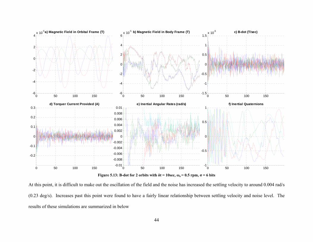
Figure 5.13: B-dot for 2 orbits with δt = 10sec, ωo = 0.5 rpm, σ = 6 bits
At this point, it is difficult to make out the oscillation of the field and the noise has increased the settling velocity to around 0.004 rad/s
(0.23 deg/s). Increases past this point were found to have a fairly linear relationship between settling velocity and noise level. The
results of these simulations are summarized in below

45
y = 108308x - 0.0345R2 = 0.9895
0.00
0.20
0.40
0.60
0.80
1.00
0.0E+00 2.0E-06 4.0E-06 6.0E-06 8.0E-06
Standard Deviation of Noise (T)
Set
tling
Rat
es (d
eg/s
)
Figure 5.14: Noise level vs. average settling rates
The graph shows the fairly strong linear relationship between noise and settling rate for standard
deviations above 6 bits (2.4e-6 T or S:N ~7:1). As mentioned earlier, this represents the
transition when the noise levels supersede the fluctuation of the local magnetic field as the
largest component of B-dot.
Because the rate of change of the magnetic field fluctuates through the spacecraft orbit,
performance can be improved by using a simple convergence test algorithm. This would
examine the value of B-dot and terminate control when some minimum value was reached. In
practice, noise limits the effectiveness of this approach; however, it can be mitigated by
averaging the values of B-dot over several time steps. It was found that velocities of 0.0017
rad/s (0.10 deg/s) could be achieved for a low-noise simulation. For higher noise levels, this
method reduced the settling velocity from 0.01 rad/s (0.57 deg/s) to 0.0035 (0.20 deg/s) at a
noise level of 15 bits (6e-6 T or S:N ~3:1). The algorithm is based on the idea that even with
high levels of noise the system will randomly settle out to a low velocity eventually.

46
5.1.5 One and Two Torquers Out Performance
This section investigates how well B-dot performs in case one or more torquers fail and the
problem goes undetected. Since there is redundancy on two of the control axes, should one
torquer fail the redundant torquer could be activated to make up for it. While no system settled
with only one active torquer, it was found that settling possible with two active torquers at a
small sacrifice in settling time. Figure 5.15 below shows the results of a simulation with a faulty
torquer on the b1 axis. The results below still show the current values that the system is
attempting to provide to the inactive torquer(s).

47
0 20 40 60 80 100 120 140-6
-4
-2
0
2
4x 10⁻⁵a) Magnetic Field in Orbital Frame (T)
0 20 40 60 80 100 120 140-6
-4
-2
0
2
4x 10⁻⁵ b) Magnetic Field in Body Frame (T)
0 20 40 60 80 100 120 140-3
-2
-1
0
1
2
3x 10⁻⁶ c) B-dot (T/sec)
0 20 40 60 80 100 120 140
-0.2
-0.1
0
0.1
0.2
0.3d) Torquer Current Provided (A)
0 20 40 60 80 100 120 140-0.1
-0.05
0
0.05
0.1
0.15e) Inertial Angular Rates (rad/s)
0 20 40 60 80 100 120 140-1
-0.5
0
0.5
1f) Inertial Quaternions
Figure 5.15: B-dot for 1.5 orbits with δt = 10sec, ωo = 1 rpm, σ = 3 bits, torquer 1 inactive
With a single torquer inactive, the final settling rates are similar, but the settling time is approximately doubled. Since the torque is
perpendicular to the torquer axis, all three axes are controllable with only two torquers. The results are similar for a torquer out the
other two axes. The system is unable to settle with two torquers out, however.
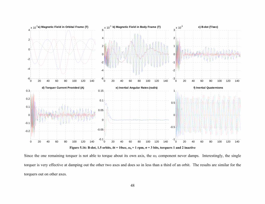
48
0 20 40 60 80 100 120 140-6
-4
-2
0
2
4x 10⁻⁵a) Magnetic Field in Orbital Frame (T)
0 20 40 60 80 100 120 140-6
-4
-2
0
2
4
6x 10⁻⁵ b) Magnetic Field in Body Frame (T)
0 20 40 60 80 100 120 140-3
-2
-1
0
1
2
3x 10⁻⁶ c) B-dot (T/sec)
0 20 40 60 80 100 120 140
-0.2
-0.1
0
0.1
0.2
0.3d) Torquer Current Provided (A)
0 20 40 60 80 100 120 140-0.1
-0.05
0
0.05
0.1
0.15e) Inertial Angular Rates (rad/s)
0 20 40 60 80 100 120 140-1
-0.5
0
0.5
1f) Inertial Quaternions
Figure 5.16: B-dot, 1.5 orbits, δt = 10sec, ωo = 1 rpm, σ = 3 bits, torquers 1 and 2 inactive
Since the one remaining torquer is not able to torque about its own axis, the ω3 component never damps. Interestingly, the single
torquer is very effective at damping out the other two axes and does so in less than a third of an orbit. The results are similar for the
torquers out on other axes.

49
Since each torquer is capable of torquing in both of its in-plane axes, the system will damp as
long as there are two orthogonal torquers active. With one torquer out, the final velocities are
comparable to the full system with an associated increase in settling time.
5.1.6 CP2 Method vs. CP3 Method
An even simpler version of B-dot which has no magnetometer calibration data is implemented on
the CP2 satellite. This method was outlined in Section 4.4.2.2. Performance was practically
identical to the calibrated version for both the high noise and high tip-off velocities. Figure 5.17
below gives an example of the CP3 method with both high noise and velocity.

50
0 20 40 60 80-6
-4
-2
0
2
4x 10⁻⁵a) Magnetic Field in Orbital Frame (T)
0 20 40 60 80-6
-4
-2
0
2
4
6x 10⁻⁵ b) Magnetic Field in Body Frame (T)
0 20 40 60 80-8
-6
-4
-2
0
2
4
6
8x 10⁻⁶ c) B-dot (T/sec)
0 20 40 60 80
-0.2
-0.1
0
0.1
0.2
0.3d) Torquer Current Provided (A)
0 20 40 60 80-0.1
0
0.1
0.2
0.3
0.4e) Inertial Angular Rates (rad/s)
0 20 40 60 80-1
-0.5
0
0.5
1f) Inertial Quaternions
Figure 5.17: CP2 B-dot for 1 orbit with δt = 4 sec, ωo = 3 rpm, σ = 6 bits
Even with a combination of high noise and initial rate, performance is nearly identical to the B-dot run with calibrated magnetometer
data. Even though CP3 would have to have the calibration data onboard, the B-dot algorithm could be simplified in order to decrease
processor load for the detumbling stage with few to no drawbacks.

51
5.1.7 B-Dot Conclusions
The B-dot algorithm was found to be very robust and could handle many types of failure with
little drop in performance. The system still settled even in with the simultaneous introduction of
high magnetometer noise, large tip-off velocities, and an inoperative torquer. It was also found
that the system has a large range of stable gains which give some leeway for incorrect moment of
inertia determination and decreases in available power. Finally, the CP2 method was found to be
nearly as effective as the CP3 method and equally as stable. The CP2 method could therefore be
implemented on CP3 if the savings in processing time were significant. If this were done,
though, it would be important to make sure that the appropriate resistors were used to minimize
the differences in offset and range between magnetometers.

52
5.2 Three-Axis Control
Even more simulations were run in order to optimize the control parameters for the three-axis
controller. The main parameters are those of the position and rate gains and pulse length, which
were found to be much more coupled than the B-dot parameters. Additionally, since the attitude
determination hardware has not yet been selected, this report will also examine what
requirements such a system might have in order to converge sufficiently. After these were
found, performance with one and two torquers out was also analyzed. Finally, the capability of
the algorithm to settle in any direction in both the orbital and inertial frames was demonstrated.
As will be shown, all of these factors are interrelated and modifications in one require that the
other parameters be re-optimized.
5.2.1 Explanation of Three-axis Plots
The results of each simulation are summarized in a single figure divided into six subplots lettered
from a-f. The current and magnetic field plots shown for B-dot were replaced with attitude-
related plots since that is the primary concern here. Furthermore, the current draw on the
torquers was extremely low, peaking at 0.1 A initially and then averaging less than 1 mA. The
x-axis of all plots is given in minutes. One may use the orbital period of approximately 95
minutes to convert these values to fractions of an orbit. With the exception of the quaternions,
the lines within each subplot represent Cartesian axes and are colored according to:
Axis 1: Blue
Axis 2: Green
Axis 3: Red

53
Axis 4: Cyan (for quaternions only)
The line types are:
• Solid: Actual values used by the simulation.
• Dashed: Desired values used by the control algorithm.
• Gray: Measured values used by control algorithm. Include discretization and noise.
An explanation of each subplot follows:
a) Quaternion Error displays the quaternion rotation between the actual and desired
quaternion vectors as defined in equation 4.5. The first three terms are used in the torque
calculation.
b) Inertial Angular Rates are the actual simulated values. See Section 2.4.2 for a definition
of the frame.
c) Inertial Quaternions. See Section 2.4.2 for a definition of the frame.
d) Pointing Error represents the error rotation angle about the quaternion error axis. It was
calculated from:
4 cos 2e
eq θ⎛ ⎞= ⎜ ⎟⎝ ⎠
Small changes in qe4 are compounded as θe approaches zero, so any noise in the
quaternion signal is extremely amplified.
e) Orbital Angular Rates. See Section 2.4.3 for a definition of the frame. These are given
for reference only and were not used directly in the error calculation.
f) Orbital Quaternions. See Section 2.4.3 for a definition of the frame. These are given for
reference only and were not used directly in the error calculation.
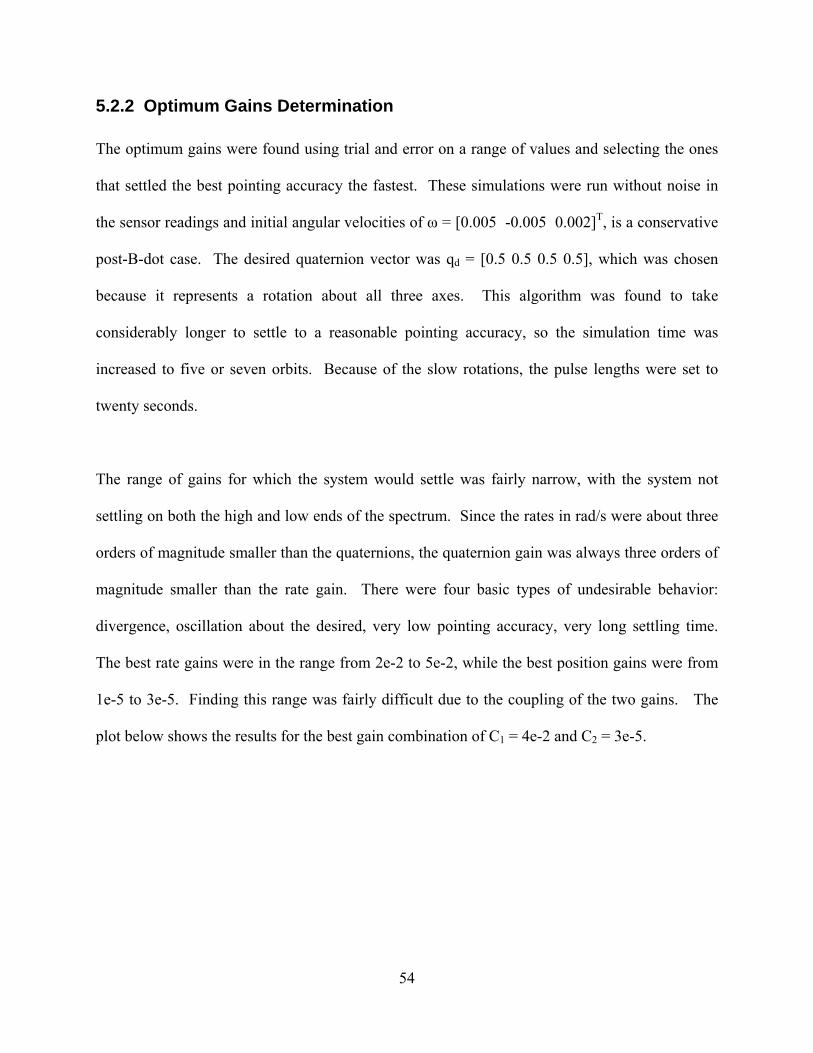
54
5.2.2 Optimum Gains Determination
The optimum gains were found using trial and error on a range of values and selecting the ones
that settled the best pointing accuracy the fastest. These simulations were run without noise in
the sensor readings and initial angular velocities of ω = [0.005 -0.005 0.002]T, is a conservative
post-B-dot case. The desired quaternion vector was qd = [0.5 0.5 0.5 0.5], which was chosen
because it represents a rotation about all three axes. This algorithm was found to take
considerably longer to settle to a reasonable pointing accuracy, so the simulation time was
increased to five or seven orbits. Because of the slow rotations, the pulse lengths were set to
twenty seconds.
The range of gains for which the system would settle was fairly narrow, with the system not
settling on both the high and low ends of the spectrum. Since the rates in rad/s were about three
orders of magnitude smaller than the quaternions, the quaternion gain was always three orders of
magnitude smaller than the rate gain. There were four basic types of undesirable behavior:
divergence, oscillation about the desired, very low pointing accuracy, very long settling time.
The best rate gains were in the range from 2e-2 to 5e-2, while the best position gains were from
1e-5 to 3e-5. Finding this range was fairly difficult due to the coupling of the two gains. The
plot below shows the results for the best gain combination of C1 = 4e-2 and C2 = 3e-5.

55
0 100 200 300 400-0.6
-0.4
-0.2
0
0.2
0.4
0.6
0.8
1a) Quaternion Error
0 100 200 300 400-6
-4
-2
0
2
4
6x 10⁻³ b) Inertial Angular Rates (rad/s)
0 100 200 300 400-1
-0.5
0
0.5
1c) Inertial Quaternions
0 100 200 300 4000
5
10
15
20
25
30
35
40d) Pointing error (deg)
0 100 200 300 400-6
-4
-2
0
2
4
6x 10⁻³ e) Orbital Angular Rates (rad/s)
0 100 200 300 400-1
-0.5
0
0.5
1f) Orbital Quaternions
Figure 5.18: 3-axis, C1 = 4e-2, C2 = 3e-5, δt = 20sec, 5 orbits
Plot d) shows how the system settles to within 12º after approximately one orbit. The rates settle extremely rapidly, dropping to a
tenth of their original magnitude in a matter of minutes. Increasing either of the gains produces instability in the system. The next
figure shows the results for an increase in the rate gain.

56
0 50 100 150 200 250-0.6
-0.4
-0.2
0
0.2
0.4
0.6
0.8
1a) Quaternion Error
0 50 100 150 200 250-6
-4
-2
0
2
4
6x 10⁻³ b) Inertial Angular Rates (rad/s)
0 50 100 150 200 250-1
-0.5
0
0.5
1c) Inertial Quaternions
0 50 100 150 200 2500
5
10
15
20
25
30
35
40d) Pointing error (deg)
0 50 100 150 200 250-6
-4
-2
0
2
4
6x 10⁻³ e) Orbital Angular Rates (rad/s)
0 50 100 150 200 250-1
-0.5
0
0.5
1f) Orbital Quaternions
Figure 5.19: 3-axis, C1 = 5e-2, C2 = 3e-5, δt = 20sec, 3 orbits
This is an example of divergent behavior. In this case, the rate gain was incremented to 5e-2, which created eventual instability as the
quaternions approached their target. A rate gain of 5e-2 can be stabilized, however, if the position gain is dropped to 2e-5 or lower.
Rate gains of 6e-2 and higher though are always unstable. Instability can also occur if the gains are too low.

57
0 100 200 300 400-1
-0.5
0
0.5
1a) Quaternion Error
0 100 200 300 400-6
-4
-2
0
2
4
6x 10⁻³ b) Inertial Angular Rates (rad/s)
0 100 200 300 400-1
-0.5
0
0.5
1c) Inertial Quaternions
0 100 200 300 4000
10
20
30
40
50
60d) Pointing error (deg)
0 100 200 300 400-6
-4
-2
0
2
4
6x 10⁻³ e) Orbital Angular Rates (rad/s)
0 100 200 300 400-1
-0.5
0
0.5
1f) Orbital Quaternions
Figure 5.20: 3-axis, C1 = 2e-2, C2 = 1e-5, δt = 20sec, 5 orbits
Here the rate gain seems to be acceptable; however, the position gain is just not high enough to induce the system to settle to a
reasonable pointing accuracy. This system might benefit from the addition of a position error integrator. If the gains are set too high,
though, the system can also develop a rate oscillation that refuses to damp out.

58
0 100 200 300 400-1
-0.5
0
0.5
1a) Quaternion Error
0 100 200 300 400-6
-4
-2
0
2
4
6x 10⁻³ b) Inertial Angular Rates (rad/s)
0 100 200 300 400-1
-0.5
0
0.5
1c) Inertial Quaternions
0 100 200 300 4000
10
20
30
40
50
60d) Pointing error (deg)
0 100 200 300 400-6
-4
-2
0
2
4
6x 10⁻³ e) Orbital Angular Rates (rad/s)
0 100 200 300 400-1
-0.5
0
0.5
1f) Orbital Quaternions
Figure 5.21: 3-axis, C1 = 2e-2, C2 = 2e-5, δt = 20sec, 5 orbits
Incrementing the position gain independently of the rate gain caused the system to start circling about the desired position at a distance
of about 45º. While neither gain is particularly high, together they are too high for the system to handle. Even though the system does
not blow up entirely, it is clear that it will never approach the desired either.

59
0 100 200 300 400-0.6
-0.4
-0.2
0
0.2
0.4
0.6
0.8
1a) Quaternion Error
0 100 200 300 400-6
-4
-2
0
2
4
6x 10⁻³ b) Inertial Angular Rates (rad/s)
0 100 200 300 400-1
-0.5
0
0.5
1c) Inertial Quaternions
0 100 200 300 4000
5
10
15
20
25
30
35
40d) Pointing error (deg)
0 100 200 300 400-6
-4
-2
0
2
4
6x 10⁻³ e) Orbital Angular Rates (rad/s)
0 100 200 300 400-1
-0.5
0
0.5
1f) Orbital Quaternions
Figure 5.22: 3-axis, C1 = 4e-2, C2 = 3e-5, δt = 20sec, 5 orbits, 3º shutoff
Returning to the best gains of C1 = 4e-2 and C2 = 3e-5, accuracy can be improved upon even further by using an algorithm similar to
the one used for B-dot. This algorithm deactivates controller once the spacecraft is pointed within a certain limit of the target and then
reactivates it as the spacecraft drifts off-target. The results are shown for a cutoff value of 3º. Compare to Figure 5.18.

60
The table below summarizes the results of the gain optimization work.
Table 5.1: Three-axis gain investigation
Rate Gain (C1)
Position Gain (C2)
Settling Time (min) Accuracy (deg)
2e-2 2e-1 qe won’t close C2 too low 2e-2 2e-5 Rates oscillate C1 too low 3e-2 1e-5 Extremely slow C2 too low 3e-2 2e-5 260 11 3e-2 3e-5 Diverges Combo too high 4e-2 1e-5 Diverges C2 too low 4e-2 2e-5 180 15 4e-2 3e-5 210 10 4e-2 4e-5 Diverges C2 too high 5e-2 2e-5 200 13 5e-2 3e-5 Diverges Combo too high 6e-2 1e-5 Diverges C1 too high
This table shows the upper and lower boundaries of the acceptable gain range. In conclusion, the
gains are highly coupled to each other, and it is important to have both at appropriate values.
Also, since the range for which the system converges is so narrow, it is important that the
moments of inertia of the spacecraft be accurately determined. Additionally, the shutoff
algorithm had some success at making previously unstable gain values stable, especially for the
noisy signals discussed in Section 5.2.5 below.
5.2.3 Optimum Pulse Time Determination
Unlike B-dot, there is a large amount of coupling between both the gains and pulse time. All
three parameters have an effect on stability, settling time, and pointing accuracy, so the optimum
combination had to be found for all three parameters at once. Since the angular rates are all very

61
small at this point, B-dot’s problem where the field changed too much during long pulse times
does not apply. Instead, long pulse times cause the system to drift back and forth across its goal
too much for it to settle. For this analysis, the pulse time was varied to find the lowest pointing
error. The optimum gain of the previous section was used, as well as the same initial velocities
representative of a post-B-dot scenario. For this gain setup, the best pulse length was
approximately 17 seconds, and the results are shown below.

62
0 50 100 150 200 250 300 350-0.6
-0.4
-0.2
0
0.2
0.4
0.6
0.8
1a) Quaternion Error
0 50 100 150 200 250 300 350-6
-4
-2
0
2
4
6x 10⁻³ b) Inertial Angular Rates (rad/s)
0 50 100 150 200 250 300 350-1
-0.5
0
0.5
1c) Inertial Quaternions
0 50 100 150 200 250 300 3500
5
10
15
20
25
30
35
40d) Pointing error (deg)
0 50 100 150 200 250 300 350-6
-4
-2
0
2
4
6x 10⁻³ e) Orbital Angular Rates (rad/s)
0 50 100 150 200 250 300 350-1
-0.5
0
0.5
1f) Orbital Quaternions
Figure 5.23: 3-axis, C1 = 4e-2, C2 = 3e-5, δt = 17sec, 4 orbits, 3º shutoff
While this is not a large improvement on the 20 or 15 second cases, the steady-state condition for 17 seconds has the mildest
oscillation. Without any noise in the system, the best pointing accuracy achievable is about 8º -9º with errors as low as 2º for brief
periods. Decreasing the pulse time below harms accuracy as shown below for a simulation with 10 second pulses.

63
0 100 200 300 400-0.6
-0.4
-0.2
0
0.2
0.4
0.6
0.8
1a) Quaternion Error
0 100 200 300 400-6
-4
-2
0
2
4
6x 10⁻³ b) Inertial Angular Rates (rad/s)
0 100 200 300 400-1
-0.5
0
0.5
1c) Inertial Quaternions
0 100 200 300 4000
5
10
15
20
25
30
35
40d) Pointing error (deg)
0 100 200 300 400-6
-4
-2
0
2
4
6x 10⁻³ e) Orbital Angular Rates (rad/s)
0 100 200 300 400-1
-0.5
0
0.5
1f) Orbital Quaternions
Figure 5.24: 3-axis, C1 = 4e-2, C2 = 3e-5, δt = 10sec, 5 orbits, 3º shutoff
Here, as the spacecraft approaches the desired point, it cannot close the gap even though the rates are very low. One possible
explanation is that with the rates low the short pulses do not have time to do their job before being recalculated.

64
The results of the pulse length investigation are summarized in the table below.
Table 5.2: Results of Pulse Length Variation
Pulse Length (sec)
Settling Time (sec)
Pointing Accuracy (deg)
5 100 2110 120 1415 160 817 160 820 210 1025 Unstable 180
The 17 seconds selected as the optimum lies in the middle of the saddle between unstable and
low accuracy. This is the value that will be used for the remainder of the experiments.
5.2.4 Effect of Sensor Resolution
This section is an exploration of the requirements for accuracy necessary for three-axis control
rather than a simulation of actual hardware. Not only is this thesis designed to be generally
applied, but at the time of writing the sensors for CP3 had not been selected nor their capabilities
explored. For this experiment, the resolutions δq and δω from equation 4.3 were modified while
the standard deviations of the noise levels were kept small. The same initial velocity and pulse
lengths as the previous section were used. The results were fairly predictable; the lower the
resolution, the higher the pointing error until the system could no longer stabilize. Working on
each sensor individually, the lowest rate resolution for which the system settled was 1e-3 rad/s
(0.057 deg/s).
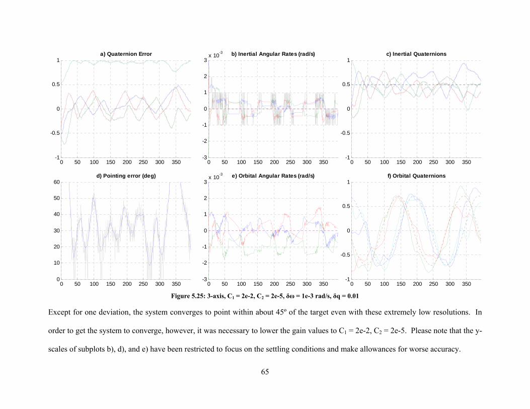
65
0 50 100 150 200 250 300 350-1
-0.5
0
0.5
1a) Quaternion Error
0 50 100 150 200 250 300 350-3
-2
-1
0
1
2
3x 10⁻³ b) Inertial Angular Rates (rad/s)
0 50 100 150 200 250 300 350-1
-0.5
0
0.5
1c) Inertial Quaternions
0 50 100 150 200 250 300 3500
10
20
30
40
50
60d) Pointing error (deg)
0 50 100 150 200 250 300 350-3
-2
-1
0
1
2
3x 10⁻³ e) Orbital Angular Rates (rad/s)
0 50 100 150 200 250 300 350-1
-0.5
0
0.5
1f) Orbital Quaternions
Figure 5.25: 3-axis, C1 = 2e-2, C2 = 2e-5, δω = 1e-3 rad/s, δq = 0.01
Except for one deviation, the system converges to point within about 45º of the target even with these extremely low resolutions. In
order to get the system to converge, however, it was necessary to lower the gain values to C1 = 2e-2, C2 = 2e-5. Please note that the y-
scales of subplots b), d), and e) have been restricted to focus on the settling conditions and make allowances for worse accuracy.

66
0 50 100 150 200 250 300 350-1
-0.5
0
0.5
1a) Quaternion Error
0 50 100 150 200 250 300 350-3
-2
-1
0
1
2
3x 10⁻³ b) Inertial Angular Rates (rad/s)
0 50 100 150 200 250 300 350-1
-0.5
0
0.5
1c) Inertial Quaternions
0 50 100 150 200 250 300 3500
10
20
30
40
50
60d) Pointing error (deg)
0 50 100 150 200 250 300 350-3
-2
-1
0
1
2
3x 10⁻³ e) Orbital Angular Rates (rad/s)
0 50 100 150 200 250 300 350-1
-0.5
0
0.5
1f) Orbital Quaternions
Figure 5.26: 3-axis, C1 = 4e-2, C2 = 3e-5, δω = 0.01 deg/s, δq = 0.01
Pulling back from the extreme case above, the lowest resolution for which the original gains settled was approximately 0.01 deg/s
(1.8e-4 rad/s). Even with this low resolution the pointing accuracy only suffers by about 10º and settling time is lowered to within one
orbit. The next figure illustrates how much more forgiving the controller is of extremely low quaternion resolutions.

67
0 50 100 150 200 250 300 350-1
-0.5
0
0.5
1a) Quaternion Error
0 50 100 150 200 250 300 350-3
-2
-1
0
1
2
3x 10⁻³ b) Inertial Angular Rates (rad/s)
0 50 100 150 200 250 300 350-1
-0.5
0
0.5
1c) Inertial Quaternions
0 50 100 150 200 250 300 3500
10
20
30
40
50
60d) Pointing error (deg)
0 50 100 150 200 250 300 350-3
-2
-1
0
1
2
3x 10⁻³ e) Orbital Angular Rates (rad/s)
0 50 100 150 200 250 300 350-1
-0.5
0
0.5
1f) Orbital Quaternions
Figure 5.27: 3-axis, C1 = 4e-2, C2 = 3e-5, δω = 1e-4 rad/s, δq = 0.5
In this simulation, the quaternions are rounded to 0.5 meaning there are only five possible values for each component. This made it
impossible for the system to close the gap, but it was at lest stable with an accuracy of about 45º. Combining the digitization of both
sensors at more reasonable values produced the following results.

68
0 50 100 150 200 250 300 350-1
-0.5
0
0.5
1a) Quaternion Error
0 50 100 150 200 250 300 350-3
-2
-1
0
1
2
3x 10⁻³ b) Inertial Angular Rates (rad/s)
0 50 100 150 200 250 300 350-1
-0.5
0
0.5
1c) Inertial Quaternions
0 50 100 150 200 250 300 3500
10
20
30
40
50
60d) Pointing error (deg)
0 50 100 150 200 250 300 350-3
-2
-1
0
1
2
3x 10⁻³ e) Orbital Angular Rates (rad/s)
0 50 100 150 200 250 300 350-1
-0.5
0
0.5
1f) Orbital Quaternions
Figure 5.28: 3-axis, C1 = 4e-2, C2 = 3e-5, δω = 0.01 deg/s, δq = 0.1
This figure shows that with reasonably precise sensors, pointing accuracies in 10-15 degree range are not unreasonable. Additionally,
precise rate knowledge is much more critical to stability than position information is.

69
5.2.5 Effect of Sensor Noise
As mentioned for B-dot, the magnetometers were found to be practically noise free, and the
simulation of their noise represents magnetic interference from operating components. The
instruments used for attitude determination under consideration would not influenced by
electromagnetic fields the way that magnetometers are, so fairly low noise levels should be
achievable for the attitude information. Ideally, a Kalman filter would also be implemented to
further reduce this noise. The experiment was run by increasing the value of the standard
deviation of the noise, σ, from equation 4.3. The same initial velocities and pulse times were
used as for previous simulations and the shutoff algorithm was employed to mitigate noise
problems. The resolutions were set to 1e-4 rad/s (0.006 deg/s) for the rates and 0.1 for the
quaternions.
As with resolution, it was found that low rates noise was more important than low position noise.
The next figure shows the results of a simulation run with medium noise levels for both rate and
position using the optimum gains found earlier.

70
0 50 100 150 200 250 300 350-1
-0.5
0
0.5
1a) Quaternion Error
0 50 100 150 200 250 300 350-3
-2
-1
0
1
2
3x 10⁻³ b) Inertial Angular Rates (rad/s)
0 50 100 150 200 250 300 350-1
-0.5
0
0.5
1c) Inertial Quaternions
0 50 100 150 200 250 300 3500
10
20
30
40
50
60d) Pointing error (deg)
0 50 100 150 200 250 300 350-3
-2
-1
0
1
2
3x 10⁻³ e) Orbital Angular Rates (rad/s)
0 50 100 150 200 250 300 350-1
-0.5
0
0.5
1f) Orbital Quaternions
Figure 5.29: 3-axis, C1 = 4e-2, C2 = 3e-5, δω = 1e-4 rad/s, δq = 0.1, σω = 2e-4 rad/s, σq = 0.1
Even with signal-to-noise ratios (S:N) of about 3:1, the system settles to within about 20º after one orbit. Increasing the rate noise
beyond this level causes the spacecraft to go unstable and increasing the position noise causes it to settle with an error greater than 60º.
By lowering the gain, however, the system is capable of handling even more noise.

71
0 50 100 150 200 250 300 350-1
-0.5
0
0.5
1a) Quaternion Error
0 50 100 150 200 250 300 350-3
-2
-1
0
1
2
3x 10⁻³ b) Inertial Angular Rates (rad/s)
0 50 100 150 200 250 300 350-1
-0.5
0
0.5
1c) Inertial Quaternions
0 50 100 150 200 250 300 3500
10
20
30
40
50
60d) Pointing error (deg)
0 50 100 150 200 250 300 350-3
-2
-1
0
1
2
3x 10⁻³ e) Orbital Angular Rates (rad/s)
0 50 100 150 200 250 300 350-1
-0.5
0
0.5
1f) Orbital Quaternions
Figure 5.30: 3-axis, C1 = 3e-2, C2 = 2e-5, δω = 1e-4 rad/s, δq = 0.1, σω = 4e-4 rad/s, σq = 0.2
Incrementing the gains down allowed the introduction of extremely unlikely levels of noise with S:N of nearly 1:1. Even so, the
system was able to point within 30º of the target. Note that the accuracy oscillates at the orbital period with valleys near the equator.
The control law was also able to handle even larger noise levels for each sensor type individually, just not both at the same time.

72
0 50 100 150 200 250 300 350-1
-0.5
0
0.5
1a) Quaternion Error
0 50 100 150 200 250 300 350-3
-2
-1
0
1
2
3x 10⁻³ b) Inertial Angular Rates (rad/s)
0 50 100 150 200 250 300 350-1
-0.5
0
0.5
1c) Inertial Quaternions
0 50 100 150 200 250 300 3500
10
20
30
40
50
60d) Pointing error (deg)
0 50 100 150 200 250 300 350-3
-2
-1
0
1
2
3x 10⁻³ e) Orbital Angular Rates (rad/s)
0 50 100 150 200 250 300 350-1
-0.5
0
0.5
1f) Orbital Quaternions
Figure 5.31: 3-axis, C1 = 3e-2, C2 = 2e-5, δω = 1e-4 rad/s, δq = 0.1, σω = 5e-4 rad/s, σq = 0.01
The gain of Figure 5.30 was better at handling high rate noise and was used for the above simulation. With the quaternion noise
minimized, it was able to handle rate noise with S:N of 1:1.5.
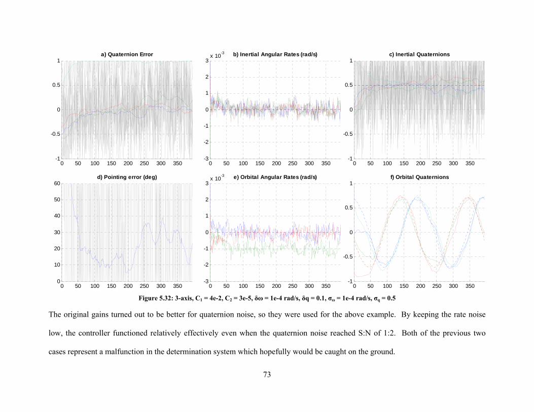
73
0 50 100 150 200 250 300 350-1
-0.5
0
0.5
1a) Quaternion Error
0 50 100 150 200 250 300 350-3
-2
-1
0
1
2
3x 10⁻³ b) Inertial Angular Rates (rad/s)
0 50 100 150 200 250 300 350-1
-0.5
0
0.5
1c) Inertial Quaternions
0 50 100 150 200 250 300 3500
10
20
30
40
50
60d) Pointing error (deg)
0 50 100 150 200 250 300 350-3
-2
-1
0
1
2
3x 10⁻³ e) Orbital Angular Rates (rad/s)
0 50 100 150 200 250 300 350-1
-0.5
0
0.5
1f) Orbital Quaternions
Figure 5.32: 3-axis, C1 = 4e-2, C2 = 3e-5, δω = 1e-4 rad/s, δq = 0.1, σω = 1e-4 rad/s, σq = 0.5
The original gains turned out to be better for quaternion noise, so they were used for the above example. By keeping the rate noise
low, the controller functioned relatively effectively even when the quaternion noise reached S:N of 1:2. Both of the previous two
cases represent a malfunction in the determination system which hopefully would be caught on the ground.

74
It was found that performance under noisy conditions could be improved by lowering the gains,
but a minor drop in pointing accuracy. The optimum gains from earlier of C1 = 4e-2 and C2 =
3e-5 were unable to handle much noise in the rates, so the gains were pulled back to C1 = 3e-2
and C2 = 2e-5. These were much more robust against noise in the rates and good enough for
quaternion noise. One benefit of the loss in pointing accuracy was that the system was able to
reach its relatively steady state much faster. This means that if pointing requirements are relaxed
slew time can be greatly improved. Additionally, the system would periodically reach pointing
errors of less than 10º even with extremely noisy signals. For example, if one wanted to take a
picture of a particular star and determination were fairly accurate, one could create a subroutine
that only took the picture once the pointing error was within an acceptable threshold.
5.2.6 One and Two Torquers Out Performance
Next was examined the failure case of one or more torquers failing and the problem going
undetected. Since there is redundancy on two of the control axes, should one torquer fail the
redundant torquer could be activated to make up for it. While no system settled with only one
active torquer, it was found that settling possible with one inactive torquer. In fact, while there
was a slight increase in settling time, pointing accuracy was often improved with a torquer out.
The stability of the malfunctioning system depended highly on the desired orientation. For
instance, Figure 5.33 below shows a simulation with the axis 2 torquer out.

75
0 100 200 300 400 500 600-1
-0.5
0
0.5
1a) Quaternion Error
0 100 200 300 400 500 600-3
-2
-1
0
1
2
3x 10⁻³ b) Inertial Angular Rates (rad/s)
0 100 200 300 400 500 600-1
-0.5
0
0.5
1c) Inertial Quaternions
0 100 200 300 400 500 6000
10
20
30
40
50
60
70
80
90d) Pointing error (deg)
0 100 200 300 400 500 600-3
-2
-1
0
1
2
3x 10⁻³ e) Orbital Angular Rates (rad/s)
0 100 200 300 400 500 600-1
-0.5
0
0.5
1f) Orbital Quaternions
Figure 5.33: 3-axis, C1 = 3e-2, C2 = 2e-5, 7 orbits, b2 torquer out
As can be seen in the figure, stability and accuracy are actually improved by deactivating the second torquer axis. The same is true
when the third axis is set to zero. Since each torquer torques about both in-plane axes, the improved performance may be due to less
interference between torquers. If the first axis torquer is deactivated, however, accuracy is dramatically decreased.

76
0 100 200 300 400 500 600-1
-0.5
0
0.5
1a) Quaternion Error
0 100 200 300 400 500 600-3
-2
-1
0
1
2
3x 10⁻³ b) Inertial Angular Rates (rad/s)
0 100 200 300 400 500 600-1
-0.5
0
0.5
1c) Inertial Quaternions
0 100 200 300 400 500 6000
10
20
30
40
50
60
70
80
90d) Pointing error (deg)
0 100 200 300 400 500 600-3
-2
-1
0
1
2
3x 10⁻³ e) Orbital Angular Rates (rad/s)
0 100 200 300 400 500 600-1
-0.5
0
0.5
1f) Orbital Quaternions
Figure 5.34: 3-axis, C1 = 3e-2, C2 = 2e-5, b1 torquer out
While the system is not entirely unstable, it does have a tendency to periodically spike away from the desired. This problem can be
alleviated by using a different desired vector. It is not entirely clear why this occurs, but it is probably related to the rotation of the
local magnetic field as the spacecraft orbits and which direction the inactive axis is attempting to point towards.

77
It was found that the system is capable of handling the failure of any one of the torquers and still
achieving accuracies similar to the fully functional state. Certain torque axes are required for
complete stability about certain orientations though, so with a failed torquer not all desired
orientations are possible. Conversely, certain orientations experienced an increase in pointing
accuracy due to torquer failure. Further study should be made into this phenomenon in order to
investigate its possible usefulness in increasing stability as well as to investigate the interaction
between the spacecraft and magnetic field.
5.2.7 Commanding Different Quaternions
Although it has not yet been demonstrated, the controller has the capability of pointing the
spacecraft to any direction in either the orbital or inertial frames. The desired orientation had
little effect on the settling time or pointing accuracy in all cases except for the torquer out case
above. Figure 5.35 below demonstrates how the system performs similarly with a different
desired orientation. It also was done for the axis 1 torquer out to illustrate how the desired
orientation and the axis of the inactive torquer relate to settling.

78
0 50 100 150 200 250 300 350-1
-0.5
0
0.5
1a) Quaternion Error
0 50 100 150 200 250 300 350-3
-2
-1
0
1
2
3x 10⁻³ b) Inertial Angular Rates (rad/s)
0 50 100 150 200 250 300 350-1
-0.5
0
0.5
1c) Inertial Quaternions
0 50 100 150 200 250 300 3500
10
20
30
40
50
60d) Pointing error (deg)
0 50 100 150 200 250 300 350-3
-2
-1
0
1
2
3x 10⁻³ e) Orbital Angular Rates (rad/s)
0 50 100 150 200 250 300 350-1
-0.5
0
0.5
1f) Orbital Quaternions
Figure 5.35: 3-axis, same parameters as Figure 5.34, qd =[ ]2 2 0 0 2 2
This desired vector represents a rotation of 90º about the b1 axis so that the b1 axis is still aligned with the i1 axis. In the previous,
unstable version of Figure 5.34, the desired vector had the b1 axis aligned with the –i2 axis. As before, the system settles to less than
10º within two orbits.
79
5.2.8 Commanding in the Orbital Frame
The controller also has the capability of commanding a rotation so that it aligns with points in the
orbital frame. This would allow Earth-related experiments to occur or the usage of a high gain
antenna for increased bandwidth. In general, performance was similar to that in the inertial
frame as long as the gains were slightly lowered. By lowering the gains, similar settling errors
were achieved at a trade off of slightly longer settling times.
Commands in the orbital frame were even more susceptible to low resolutions and high noise
levels than in the inertial frame, probably because a non-zero angular velocity and constantly
changing desired quaternion vector are required.

80
0 100 200 300 400 500 600-1
-0.5
0
0.5
1a) Quaternion Error
0 100 200 300 400 500 600-3
-2
-1
0
1
2
3x 10⁻³ b) Inertial Angular Rates (rad/s)
0 100 200 300 400 500 600-1
-0.5
0
0.5
1c) Inertial Quaternions
0 100 200 300 400 500 6000
10
20
30
40
50
60d) Pointing error (deg)
0 100 200 300 400 500 600-3
-2
-1
0
1
2
3x 10⁻³ e) Orbital Angular Rates (rad/s)
0 100 200 300 400 500 600-1
-0.5
0
0.5
1f) Orbital Quaternions
Figure 5.36: Orbital frame, C1 = 2e-2, C2 = 1e-5
With the relatively high noise levels here, the system needs a full seven orbits to settle. Response time can be improved to
approximately one orbit with improved sensor accuracy and precision as shown below.

81
0 100 200 300 400-1
-0.5
0
0.5
1a) Quaternion Error
0 100 200 300 400-3
-2
-1
0
1
2
3x 10⁻³ b) Inertial Angular Rates (rad/s)
0 100 200 300 400-1
-0.5
0
0.5
1c) Inertial Quaternions
0 100 200 300 4000
10
20
30
40
50
60d) Pointing error (deg)
0 100 200 300 400-3
-2
-1
0
1
2
3x 10⁻³ e) Orbital Angular Rates (rad/s)
0 100 200 300 400-1
-0.5
0
0.5
1f) Orbital Quaternions
Figure 5.37: Orbital frame, C1 = 3e-2, C2 = 2e-5
With the resolutions from Figure 5.25 and fairly low noise levels, the system settles accuracies of about 15º in the orbital frame. The
differences may also just be due to additional error introduced by the frame transformation of the desired vector. In that case it would
just be a numerical artifact of the simulation and would not happen in the real world.

82
5.2.9 Three-Axis Conclusions
The controller was found to be much more sensitive to changes in any of the three control
parameters, position gain, rate gain, and pulse time. All three parameters are coupled and must
be optimized simultaneously. It is also important to know the spacecraft moments of inertia
accurately for the simulated gains to apply. The algorithm performed well with low sensor
resolutions, but the rate information was more critical than position. Dropping the resolution, of
course, brought an inherent drop in accuracy. The system responded very well to noise and was
able to maintain stability with signal-to-noise ratios in the 2:1 range. Controllability was limited
when one torquer failed in that settling and accuracy depended on the desired orientation.
Current consumption was very low, averaging less than 1/100th the torquer ability, so the system
should be able to handle the disturbance torques that were not included. In a fully functional
satellite with reasonably good resolutions and low noise, accuracies of 10º-20º should be
achievable. Even so, the pointing error periodically dropped below 5º, so an algorithm could be
written that waited for accuracy to increase before performing the experiment, taking a picture
for example.
5.3 Comparison of B-dot and Three-Axis Controllers
In general, B-dot was a much simpler, more robust algorithm that could handle several
simultaneous failures with relatively little drop in performance. The three-axis algorithm was
much more complicated and susceptible to failure. The responses were highly non-linear and
generally not intuitively predictable. On the other hand, it did have a relatively good response to

83
extremely unlikely resolutions and noise levels. The table below summarizes the differences
between the two algorithms.
Table 5.3: Comparison of B-dot and three-axis algorithms
B-dot Three-axis Calculation steps 3 5/7 steps
Calculation type Arithmetic Matrix algebra
Gain sensitivity Low High
Calc. frequency 2-10 sec 15-25 sec
Settling time <1 orbit Up to 5 orbits
Ave current draw 100-200 mA <1mA
Noise Response Great Good
Torquer out Unaffected Ltd controllability
Main Strength Fail-safe Accuracy
In comparing them, it is important to remember that both algorithms are necessary for a complete
controller package. The three-axis controller is not designed to work with high rates, while B-
dot is not capable of achieving and level of pointing accuracy.

84
6 FUTURE WORK
While hopefully this thesis has answered several questions, it has raised several more, and there
is still much more investigation to be done. There are a few hardware-related experiments whose
data would improve simulation accuracy. This value could then be plugged into the simulation
for disturbance torque calculation. First, its mass moments of inertia and principal angles could
be determined either through measurement or improving the accuracy of the solid model.
Second, the sensor models for the rates and quaternions should be refined once the actual
hardware is chosen. Finally, the spacecraft’s residual magnetic dipole while in a power-on
operational state could be measured. Simulation accuracy could be improve by including the
remaining principal disturbance torques.
Further investigation should be made into improving the three-axis control algorithm.
Hopefully, some form of numerical position error integration feedback can be found that would
improve the steady state performance. The problem with such a system would be finding a
method that is capable of being implemented with the limited computing power available
onboard. Additionally, the periodic fluctuation of the magnetic field varied effective gain which
in turn caused an oscillation in the pointing accuracy. This problem might be mitigated by
making the gains a function of the local magnetic field vector. Finally, as the spacecraft settles
out near the desired orientation, the system becomes linear enough that this type of analysis is
valid. A third controller could be developed based on linear control theory which would take
over for additional pointing refinement.

85
Even with the simulation the way it is, there is more research to be done. The magnetorquer
current information could be used power consumption analysis to help refine the satellite’s
power budget. Also, the torquer-out performance was not completely explored here. The
apparent performance enhancement for some orientations should be investigated. Perhaps a two-
torquer system could be used intentionally where the deactivated torquer is chosen based on the
desired orientation. Finally, upon completion of the determination simulation, this work should
be merged with it into one coherent ADCS simulation.

86
BIBLIOGRAPHY
1. Wertz, James R., ed. Spacecraft Attitude Dynamics and Control. El Segundo, CA: Kluwer Academic Publishers, 1978.
2. International Geomagnetic Reference Field (IGRF). Accessed June 10, 2005; Revised
March 22, 2005; available from http://www.ngdc.noaa.gov/IAGA/vmod/igrf.html. 3. Wertz, James R., and Wiley J. Larson, eds. Space Mission Analysis and Design (SMAD)
3rd Edition. El Segundo, CA: Microcosm Press, 1999. 4. Svartveit, Kristian. “Attitude Determination of the NCUBE Satellite.” Thesis prepared
for NTNU, Norway: June 2003. 5. Graversen, Torben, et al. “Attitude Control System for AAU CubeSat.” Thesis prepared
for Aalborg University, Denmark: 6 June 2002. 6. Guelman, M., et al. “Design and Testing of Magnetic Controllers for Satellite
Stabilization.” Acta Astronautica Vol. 56 (2005): 231-239. 7. Tivey, Maurice A., “Ocean Bottom Magnetology Laboratory: Magnetic Analysis Code.”
Accessed June 10, 2005; Revised April 2005; available from http://deeptow.whoi.edu/matlab.html.
8. Sidi, Marcel J. Spacecraft Dynamics and Control. Cambridge: Cambridge University
Press, 2000.

87
Appendix A: Magfd.m
This is the program developed by Maurice Tivey at the Woods Hole Marine Magnetism Group7
which returns the estimated magnetic field vector at any point in space and time based on the
IGRF-10 developed by the IAGA.2
function J=magfd(DATE,ITYPE,ALT,COLAT,ELONG) % MAGFD % Function to compute Earths magnetic field % and components: X,Y,Z,T for a given latitude % and longitude, date and altitude. % Uses MATLAB MAT files sh1900.mat to sh2005.mat in 5 yr % intervals. % % Usage: out=magfd(DATE,ITYPE,ALT,COLAT,ELONG); % % DATE = date of survey (decimal years) % ITYPE=1 for geodetic to geocentric (USE 1) % ALT = altitude of survey relative to sealevel (km +ve up) % COLAT=90-latitude (decimal degrees) % ELONG=longitude of survey (decimal degrees) % % Output array out contains components X,Y,Z,T in nanoteslas % X north component % Y east component % Z vertical component +ve down % T total field magnitude % % ref: IAGA, Division V, Working Group 8, % International geomagnetic reference field, 1995 % revision, Geophys. J. Int, 125, 318-321, 1996. % IGRF2000 % IAGA Working Group V-8 (Chair: Mioara Mandea, Institut de % Physique du Globe de Paris, 4 Place Jussieu, 75252 Paris, % France. Fax:33 238 339 504, email: [email protected]). % http://www.dsri.dk/Oersted/Field_models % % Maurice A. Tivey March 1997 % Mod Dec 1999 (add igrf2000 and y2k compliance % Mod Nov 2000 (use up to degree 10 sh coefficients) % Mod Apr 2005 added 2005 coeffs % http://deeptow.whoi.edu/matlab.html % Copyright: Maurice A. Tivey, 2005 % Woods Hole Oceanographic Institution if nargin < 1 disp('DEMO MAGFD:') help magfd disp('Compute magnetic field at Woods Hole from Jan 1st 1900'); disp(' every five years until 2005'); disp(' Latitude 42 N, Longitude 74W') disp('sample command: out=magfd(1997,1,0,90-42,-74);') for i=1:22, out(i,:)=magfd(-((i-1)*5+1900),1,0,90-42,-74);

88
end plot(([1:22]-1)*5+1900,out(:,4),'-r+','linewidth',2); xlabel('Year'); ylabel('Total Magnetic Field (nT)') title('Total Magnetic Field Intensity at Woods Hole, MA') axis tight return end %igrfyear=2000; %igrffile='sh2000'; %DGRF=[1900:5:2000]; DGRF=[1900:5:2005]; igrfyear=2005; igrffile='sh2005'; pl=0; if DATE < 0, pl=1; end DATE=abs(DATE); % Determine year for base DGRF to use. if DATE < igrfyear, BASE=fix(DATE-DGRF(1)); i=fix(BASE/5)+1; BASE=DGRF(i); if pl==0, fprintf('Using DGRF base year %f \n',BASE); end eval(['load sh',num2str(BASE)]) % loads agh and agh41 but now need to get iagh=agh;iagh41=agh41; % load next epoch eval(['load sh',num2str(DGRF(i+1))]) eagh=agh;eagh41=agh41; dgh=(eagh-iagh)./5;dgh41=(eagh41-iagh41)./5; agh=iagh;agh41=iagh41; clear iagh iagh41 eagh eagh41 T = DATE - BASE; else % if pl==0, % fprintf('Using IGRF base year %f \n',igrfyear); % end eval(['load ',igrffile]) % load in igrf data file T = DATE - igrfyear; end % combine spherical harmonic coefficients from first 8 degrees % with degrees 9 and 10 agh=[agh,agh41]; dgh=[dgh,dgh41]; % D2R = pi/180; R = ALT; ONE = COLAT*0.01745329; SLAT = cos(ONE); CLAT = sin(ONE); ONE = ELONG*0.01745329; CL(1) = cos(ONE); SL(1) = sin(ONE); X = 0.0; Y = 0.0; Z = 0.0; CD = 1.0; SD = 0.0; L = 1; M = 1; N = 0;

89
if ITYPE == 1 % CONVERSION FROM GEODETIC TO GEOCENTRIC COORDINATES A2 = 40680925.; % squared semi major axis B2 = 40408588.; % squared semi minor axis ONE = A2*CLAT*CLAT; TWO = B2*SLAT*SLAT; THREE = ONE + TWO; FOUR = sqrt(THREE); R = sqrt(ALT*(ALT + 2.0*FOUR) + (A2*ONE + B2*TWO)/THREE); CD = (ALT + FOUR)/R; SD = (A2 - B2)/FOUR*SLAT*CLAT/R; ONE = SLAT; SLAT = SLAT*CD - CLAT*SD; CLAT = CLAT*CD + ONE*SD; end RATIO = 6371.2/R; % % COMPUTATION OF SCHMIDT QUASI-NORMAL COEFFICIENTS P AND X(=Q) % P(1) = 2.0*SLAT; P(2) = 2.0*CLAT; P(3) = 4.5*SLAT*SLAT - 1.5; P(4) = 5.1961524*CLAT*SLAT; Q(1) = -CLAT; Q(2) = SLAT; Q(3) = -3.0*CLAT*SLAT; Q(4) = 1.7320508*(SLAT*SLAT - CLAT*CLAT); NMAX=10; % Max number of harmonic degrees NPQ=(NMAX*(NMAX+3))/2; for K=1:NPQ, if N < M M = 0; N = N + 1; RR = RATIO^(N + 2); FN = N; end FM = M; if K >= 5 %8,5,5 if (M-N) == 0 %,7,6,7 ONE = sqrt(1.0 - 0.5/FM); J = K - N - 1; P(K) = (1.0 + 1.0/FM)*ONE*CLAT*P(J); Q(K) = ONE*(CLAT*Q(J) + SLAT/FM*P(J)); SL(M) = SL(M-1)*CL(1) + CL(M-1)*SL(1); CL(M) = CL(M-1)*CL(1) - SL(M-1)*SL(1); else ONE = sqrt(FN*FN - FM*FM); TWO = sqrt((FN - 1.0)^2 - FM*FM)/ONE; THREE = (2.0*FN - 1.0)/ONE; I = K - N; J = K - 2*N + 1; P(K) = (FN + 1.0)*(THREE*SLAT/FN*P(I) - TWO/(FN - 1.0)*P(J)); Q(K) = THREE*(SLAT*Q(I) - CLAT/FN*P(I)) - TWO*Q(J); end % % SYNTHESIS OF X, Y AND Z IN GEOCENTRIC COORDINATES % end ONE = (agh(L) + dgh(L)*T)*RR; if M == 0 %10,9,10 X = X + ONE*Q(K); Z = Z - ONE*P(K); L = L + 1;
90
else TWO = (agh(L+1) + dgh(L+1)*T)*RR; THREE = ONE*CL(M) + TWO*SL(M); X = X + THREE*Q(K); Z = Z - THREE*P(K); if CLAT > 0 %12,12,11 Y = Y+(ONE*SL(M)-TWO*CL(M))*FM*P(K)/((FN + 1.0)*CLAT); else Y = Y + (ONE*SL(M) - TWO*CL(M))*Q(K)*SLAT; end L = L + 2; end M = M + 1; end % CONVERSION TO COORDINATE SYSTEM SPECIFIED BY ITYPE ONE = X; X = X*CD + Z*SD; Z = Z*CD - ONE*SD; T = sqrt(X*X + Y*Y + Z*Z); J=[X,Y,Z,T]; % END

91
Appendix B: CP2 Magnetometer Calibration Data
This data is based on the calibration tests performed on the flight hardware using a fluxgate
magnetometer for baseline data.
Table B.1: Calibration data for CP2 flight panels
a (T/bit) b (T) Board Face HMC1052 Axis Body Axis 4.50E-07 -5.93E-05 FVII Front A (+X) 4.29E-07 -4.75E-05 FVII Front B (+Z) 4.40E-07 -5.45E-05 SXVIII Left A (-Y) 4.33E-07 -5.26E-05 SXVIII Left B (-Z) 4.92E-07 -5.68E-05 SXX Right A (-Y) 4.61E-07 -5.79E-05 SXX Right B (+Z) 4.16E-07 -5.60E-05 SXXI Top A (-Y) 3.98E-07 -5.07E-05 SXXI Top B (-X) 4.38E-07 -5.58E-05 SXXII Bottom A (-Y) 4.26E-07 -5.50E-05 SXXII Bottom B (+X)

92
Appendix C: Orbit Propagation and Attitude Simulator
This is the code used for all the attitude simulation results in Section 5. It was originally
designed as an orbit propagator, solar panel power calculator, and B-dot simulation by fellow
graduate student Erick Sturm over the summer of 2004. The author has modified to streamline
the code and added the three-axis controller, hardware models, frame transformations, problem-
specific plots, and other modifications for enhanced functionality.
%========================================================================== %========================================================================== % Author: Erick Sturm % Date: July 2004 % Program: Polysat Orbit Propagator & Attitude Simulator %========================================================================== % Description: % This program was initially created to take the % NASA TLEs of a cubesat and use them to determine % the lat and long of the cubesat at another date. %========================================================================== % Revised: Dan Guerrant % Date: September 2004-June 05 % This version is OPAS with my bug fixes and: % 0. Minus Solar Power and Current calc. (OPASquick) % 1. 3-axis stabilization (zeros rates) (OPAS3axis1) % 2. 3-axis control (zeros quaternions/aligns body,inertial frames) % (OPAS3axis2) % 3. Allows user to input quaternions in inertial frame to point to. % (OPAS3axis3) % 4. Adds ability to point to quaternions in orbital frame. (OPAS3axis4) % 5. Bug fixes quaternion error. Attitude sim in previous versions % incorrect. Still having trouble w/ control in orbital frame. Debug % version where desired torques inputed directly into attitude sim. % (OPAS3axis5, April 05) % 6. More acurately models sensors. Omega I>O transform finally % working. Includes GG disturbance. (OPAS3axis6, June 05) % 7. Creates different plots based on control law in use. Fixed error % in current limiter. (OPAS3axisFinal, June 05) %========================================================================== function OPAS close all;warning off MATLAB:singularMatrix;%clc start = clock; %Store starting time for run time calculation %========================================================================== %Scan in the Data from the NASA TLE %========================================================================== %Specs for our supposed orbit: rp=660 ra=760 i=98 raan=22:30 fid = fopen('CP2TLE.txt','rb'); L0 = fgetl(fid); L1 = fscanf(fid,'%d%6d%*c%5d%*3c%2d%f%f%5d%*c%*d%5d%*c%*d%d%5d',[1,10]);

93
L2 = fscanf(fid,'%d%6d%f%f%f%f%f%f',[1,8]); fclose(fid); eY0 = L1(1,4); %Epoch Year eD0 = L1(1,5); %Epoch Day nD0 = L1(1,6)*4*pi/(24*3600)^2; %First Derivative of Mean Motion (rad/sec2) nD20 = L1(1,7)*12*pi/(24*3600)^3; %Second Derivative of Mean Motion (rad/sec3) D0 = L1(1,8); %Drag Term / Radiation Pressure Term i0 = L2(1,3)*pi/180; %Inclination (rads) Om0 = L2(1,4)*pi/180; %Right Ascension of the Ascending Node (rads) e0 = L2(1,5)/1e7; %Eccentricity om0 = L2(1,6)*pi/180; %Argument of Perigee (rads) M0 = L2(1,7)*pi/180; %Mean Anomaly (rads) n0 = L2(1,8)*2*pi/24/3600; %Mean Motion (rad/sec) %========================================================================== %Constants %========================================================================== Re = 6378.13649; %Equatorial Radius of the Earth (km) mu = 3.986004415e5; %Gravitational Constant of the Earth (km3/s2) we = 7.2921158553e-5; %Angular Velocity of the Earth (rad/s) oe = 0.40909262967; %Obliquity of the Eccliptic (rad) ne = 1.9909887984e-7; %Mean Motion of the Earth (rad/s) Pmax = 1; %Maximum Solar Panel Power (W) Ps = 1367; %Solar Radiation Power (W/m2) t0o = 0; %Simulation Start Time J2 = 0.00108263; %J2 Gravitational Perturbation Constant Lv = 2*pi/180; %Elevation Angle required to see the S/C (rad) %========================================================================== %Define the Final Time %========================================================================== eYd = eY0+0; %Epoch Year Desired eDd = eD0+0; %Epoch Day Desired eHd = 01; %Epoch Hour Desired eMd = 40; %Epoch Minute Desired eSd = 00; %Epoch Second Desired etf = eSd+60*(eMd+60*(eHd+24*(eDd+365.25*eYd))); %Epoch Time Final eti = 60*(60*(24*(eD0+365.25*eY0))); %Epoch Time Initial tfo = etf-eti; %Simulation Stop Time % tspano=[t0o,tfo]; %Simulation Time Span fed into ode45 %========================================================================== %Calculation of Time from Vernal Equinox %========================================================================== Yve = 04; %Epoch Year of Vernal Equinox Dve = 79; %Epoch Day of Vernal Equinox Hve = 06; %Epoch Hour of Vernal Equinox Mve = 47; %Epoch Minute of Vernal Equinox Sve = 00; %Epoch Second of Vernal Equinox tve = Sve+60*(Mve+60*(Hve+24*(Dve+365.25*Yve))); %Epoch Time of Vernal Equinox veo = 0;%-5.39; %Vernal Equinox Offset due to Equinox not happening @ 0:00 GMT dti = eti-tve; %Initial Change in Time from Vernal Equinox dtf = etf-tve; %Final Change in Time from Vernal Equinox

94
%========================================================================== %Initial Condition Calculation %========================================================================== TLE = [i0;Om0;e0;om0;M0;n0]; %TLEs Loaded above Keps = tle2keps(TLE,mu); %Convert TLEs to Keplerian Elements a0 = Keps(1); %Semi-Major Axis (km) e0 = Keps(2); %Eccentricty nu0 = Keps(3); %True Anomaly (radians) i0 = Keps(4); %Inclination (radians) Om0 = Keps(5); %RAAN (radians) om0 = Keps(6); %Arg of Perigee (radians) P0 = a0*(1-e0^2); %Semi-Lattice Rectum (km) r0 = P0/(1+e0*cos(nu0)); %Radius (km) v0 = sqrt(mu*(2/r0-1/a0)); %Velocity (km/sec) y0 = (nu0/abs(nu0))*acos((sqrt(mu*P0)/(r0*v0))); %Gamma (rad) rD0 = v0*sin(y0); %Radial Velocity (km/sec) nuD0 = v0*cos(y0)/r0; %Angular Velocity (rad/sec) state0 = [n0;nD0;a0;e0;i0;Om0;om0;nu0;nuD0;r0;rD0]; %Initial State %========================================================================== %Orbit Propagation %========================================================================== tfo = .3*pi*sqrt(a0^3/mu); %Final Time for Orbit Propagator options = odeset('RelTol', 1e-4); [to,xo] = ode45(@oDiffEq,[t0o,tfo],state0,[],mu,J2,nD20,Re); mm = xo(:,1); %Mean Motion (rad/s) nD = xo(:,2); %First Derivative of Mean Motion (rad/s2) a = xo(:,3); %Semi-Major Axis (km) e = xo(:,4); %Eccentricity i = xo(:,5); %Inclination (rad) Om = xo(:,6); %RAAN (rad) om = xo(:,7); %Arg of Perigee (rad) nu = xo(:,8); %True Anomaly (rad) nuD = xo(:,9); %Angular Velocity (rad/s) r = xo(:,10); %Radius (km) rD = xo(:,11); %Radial Velocity (km/s) %========================================================================== %Frame Transformations %========================================================================== xi=xo2xi(r,nu,om,Om,i); % Orbit 2 Inertial xe=xi2xe(xi,to,dti,we,veo); % Inertial 2 Earth rll = xe2rll(xe); % Earth 2 Lat, Long, & Radius R = rll(:,1); %Radius to S/C lat = rll(:,2); %Latitude of S/C long = rll(:,3); %Longitude of S/C %========================================================================== %Find the Magnetic Field Vector using the IGRF Model %========================================================================== BL=rllt2BL(R,lat,long,to,eti,Re); %Mag-Field in Local N,E,Nadir (Teslas) Be=xm2xe(BL,lat,long); %Mag-Field in Earth-Fixed Bi=xe2xi(Be,to,dti,we,veo); %Mag-Field in Inertial %Normalize the Mag-Field for Unit Vector Plot

95
for ndx=1:length(Bi) uBi(ndx,:)=Bi(ndx,:)/norm(Bi(ndx,:)); %Unit Mag-Field Vector in Inertial Frame end %========================================================================== %Create a Ground Track %========================================================================== %Create a Figure Window f1=figure(1); set(f1,'color','w','Renderer','zbuffer') set(f1,'Name', 'Orbital Views') set(f1,'units','normalized','position',[0 0 1 1]) % movegui(f1,'onscreen') %Create the World Map Background and Ground Track Axes World = imread('worldmap.jpg'); %Read World Map imagesc([-180 180],[90 -90],World); hold; %Plot World Map a1=gca; set(a1,'YDir','normal') grid on %Algorithm to plot the Ground Track [longm,latm]=col2mat(long,lat,i); %Convert Columns to Matrices [m,n]=size(longm); for ndx=1:n for mdx=2:m if longm(mdx,ndx)==0 & longm(mdx-1,ndx)~=0 for k=1:(mdx-1) longp(k)=longm(k,ndx); latp(k)=latm(k,ndx); end plot(longp,latp,'Linewidth',2,'Color','r') clear longp; clear latp; elseif longm(m,ndx)~=0 plot(longm(:,ndx),latm(:,ndx),'Linewidth',2,'Color','r') end end end %Find the Ground Area that can see the S/C gai=r2gai(xi,Re,Lv); %Algorithm to plot the Ground Area that can see the S/C [galo,gala]=gai2gall(gai,to,dti,we,i,veo); %Convert above to Lat & Long [m,n]=size(galo); if n>1 for ndx=1:n for mdx=2:m if galo(mdx,ndx)==0 & galo(mdx-1,ndx)~=0 for k=1:(mdx-1) galop(k)=galo(k,ndx); galap(k)=gala(k,ndx); end plot(galop,galap,'Linewidth',1.25,'Color','g') clear galop; clear galap; elseif galo(m,ndx)~=0 plot(galo(:,ndx),gala(:,ndx),'Linewidth',1.25,'Color','g') end end end

96
else plot(galo,gala,'linewidth',1.25,'Color','g'); end %Plotting Cal Poly, SLO, CA plot(-120.66512,35.30243,'rx') %Defining Ground Track Axes Properties title('Ground Track of the S/C') axis([-180 180 -90 90]) set(a1,'xtick',[-180 -165 -150 -135 -120 -105 -90 -75 -60 -45 ... -30 -15 0 15 30 45 60 75 90 105 120 135 150 165 180]) set(a1,'ytick',[-90 -75 -60 -45 -30 -15 0 15 30 45 60 75 90]) set(a1,'units','normalized','position',[.3 .2 .6 .4]) set(a1,'xcolor','k','ycolor','k') set(get(a1,'Title'),'FontWeight','bold','Color','k') %========================================================================== %Attitude Simulator %========================================================================== %S/C Properties------------------------------------------------------------ m = 1.00; %Mass (kg) l = 0.10; %Length (m) w = 0.09; %Width (m) h = 0.11; %Height (m) % I = 1/12*m*[(h^2+w^2);(l^2+h^2);(w^2+l^2)]; %Mass Moments of Inertia (kg-m^2) I = [8.817e-4; 9.804e-4; 10.35e-4]; %MMI from IDEAS model of CP2 K = [(I(2)-I(3))/I(1); (I(3)-I(1))/I(2); (I(1)-I(2))/I(3)]; %Simulation Setup---------------------------------------------------------- t0a = t0o; %Seconds to offset AtSim Start from OrProp Start tfa = tfo; %Seconds to run AtSim tr = 9.9; %Seconds taking readings dtrc = 0.1; %Seconds between reading end and control start tc = tr; %Seconds to have Torquers on [0.025,6.4] dtcr = dtrc; %Seconds between control end and reading start %Initial Conditions-------------------------------------------------------- % w0 = [0.005 -0.005 0.002]; %Conservative after BDot case (rad/s) w0 = [1*pi/30 .05 -.05]; %Worst likely deployment case q0 = [0 0 0 1]; %Initial Quaternion - Inertial->Body state0 = [w0 q0]; %Initial State %Desired State------------------------------------------------------------- frame = 0; %0 if desidred given in inertial, 1 for orbital switch 5 %Desired Quaternions (frame defined above) case 1, qd = [1 0 0 0]; %180 about b1 case 2, qd = [0 1 0 0]; %180 about b2 case 3, qd = [0 0 1 0]; %180 about b3 case 4, qd = [0 0 0 1]; %Alligned case 5, qd = [0.5 0.5 0.5 0.5]; %120 about [1 1 1] case 6, qd = [0 0 sqrt(2)/2 sqrt(2)/2]; %90 about b3 case 7, qd = [0 sqrt(2)/2 0 sqrt(2)/2]; %90 about b2 case 8, qd = [sqrt(2)/2 0 0 sqrt(2)/2]; %90 about b1 end if frame qdo = qd; %Desired Quaternions in orbital frame wdo = [0 0 0];

97
else qdi = qd; %Desired Quaternions in inertial frame wdi = [0 0 0]; end %Magnetometer Modeling Method---------------------------------------------- test = 5; %Switch selects the test case listed below switch test case 1 %Perfect 3-axis. No mag/pos/rate error, direct torquage from control law. case 2 %3-axis. No mag/pos/rate error, control torque turned into mag commands. case 3 %3-axis CP3 sim. Mag/pos/rate error, control torque to mag commands. case 4 %Perfect B-Dot sim. No mag error. case 5 %CP3 B-dot sim. Mag error. case 6 %CP2 B-dot sim. Mag error, actual mag cal data case 7 %CP2 B-dot sim. Mag error, actual mag cal data, b-dot w bits (as implimented) end if test >= 6 %Actual CP2 callibration data from Side Test Data.xls CalData = [ % m b 4.50e-7 -5.93e-5; %Front Magnetometer Axis A (+X) FVII 4.29e-7 -4.75e-5; %Front Magnetometer Axis B (+Z) 4.40e-7 -5.45e-5; %Left Magnetometer Axis A (-Y) SXVIII 4.33e-7 -5.26e-5; %Left Magnetometer Axis B (-Z) 4.92e-7 -5.68e-5; %Right Magnetometer Axis A (-Y) SXX 4.61e-7 -5.79e-5; %Right Magnetometer Axis B (+Z) 4.16e-7 -5.60e-5; %Top Magnetometer Axis A (-Y) SXXI 3.98e-7 -5.07e-5; %Top Magnetometer Axis B (-X) 4.38e-7 -5.58e-5; %Bottom Magnetometer Axis A (-Y) SXXII 4.26e-7 -5.50e-5; %Bottom Magnetometer Axis B (+X) ]; else % Ideal mag setup: 0=-500mG,128=0, 255=500mG % Tesla = m * Bit value + b CalData = [5e-5/128*ones(10,1) -5e-5*ones(10,1)]; end StDvM = 2; %Standard Deviation in Magnetometer Readings (Bits) StDvG = 5e-5; %Std Dev in gyro readings (rad/s) StDvQ = 1e-2; %Std Dev in quaternion readings from star tracker Gres = 1e-4; %Resolution of gyros(rad/s) Qres = 1e-1; %Resolution of quaternions Ires = 0.0012; %Resolution of Magnetorquer Current (Amps/Step) Ilim = 0.3; %Max current per torquer(Amps) %Controller Parameters----------------------------------------------------- N = 54; %Number of Torquer Loops A = .003; %Average Area of Torquer Loops (m^2) NA = 0.150622; %Sum of area enclosed by each loop (~N*A) C = 8e-3; %Kyle's B-Dot Constant on CP2 (~Kk*CalData(:,1)) Kk = 20e3; %C*128/5e-5; %B-Dot Controller Gain for CP3 (~C/CalData(:,1)) C1 = 20e-3; %Rate gain C2 = 10e-6; %Quaternion gain %Sim w/ Torquing----------------------------------------------------------- %Loop Initialization tas = t0a; %attitude simulation time wbri = w0; %Initial Omegas in the Body Frame during Readings

98
qri = q0; %Quaternions after torquers ndx = 1; mdx = 1; idx = 1; while tas < tfa mub=[0;0;0]; %Magnetic Dipole generated by Torquers Treq=[0;0;0]; %Attitude Sim of S/C During Readings [tar,stater]=ode45(@aDiffEq,[tas,tas+tr,tas+tr+dtrc],[wbri';qri'],... options,I,K,mub,to,Bi,Treq,test,mm); wbr=stater(:,1:3); %Omegas in the Body Frame during Readings qr =stater(:,4:7); %Quaternions during Readings wbci=wbr(end,:); %Initial Omegas in the Body Frame during Torquing qci =qr(end,:); %Initial Quaternions during Torquing % Mag-field and Attitude Measurments Bb=Bi2Bb(to,Bi,tar,qr); %Mag-Field in Body Frame during Readings (Tesla) if (test==1 | test==2 | test==4) Bbm = Bb; %Measured Mag-Field (no error) wbrn = wbr(2,:); %Measured angular rates (no error) qrn = qr(2,:); %Measured quaternions (no error) else [BbmBit,Bbm] = magErr(Bb,CalData,StDvM); %Measured Mag-Field (error introduced) wbrn = roundto(wbr(2,:)+StDvG.*randn(size(wbr(2,:))),Gres); %Measured angular rates (error introduced) qrn = roundto(qr(2,:)+StDvQ.*randn(size(qr(2,:))),Qres); %Measured quaternions (error introduced) end %Algorithm to Allow Plotting of Measured Mag-Field taBm(idx:idx+2)=tar; Bm(idx:idx+2,1:3)=Bbm;B(idx:idx+2,1:3)=Bb; idx=idx+3; %Inertial to Orbital State Vector Transformation mm1 = interp1(to,mm,tar(2)); %Mean Motion(rad/s) theta = interp1(to,nu,tar(2)); %True Anomoly(rad) qoi = [0 0 sin(theta/2) cos(theta/2)]; %Orbital>Inertial rotation qio = [0 0 sin(-theta/2) cos(-theta/2)]; %Inertial>Orbital rotation qorb(mdx,:) = qtrans(qio,qr(2,:)); %Actual state in orbital frame worb(mdx,:) = wi2wo(wbr(2,:),qr(2,:),mm1); %Actual rates in orbital frame %%%%%%%%%%%%%%%%% Controllers %%%%%%%%%%%%%%%%% %%%%%%%%%%%%%% 3-axis controller %%%%%%%%%%%%%% %Find the error if frame %Converts desired vector from orbital to inertial qdi = qtrans(qoi,qdo); %Desired quaternions in inertial frame wdi = wo2wi(wdo,qdo,mm1); %Desired rates in inertial frame else %Converts desired vector from inertial to orbital qdo = qtrans(qio,qdi); %Desired quaternions in orbital frame wdo = wi2wo(wdi,qdi,mm1); %Desired rates in orbital frame end qea(mdx,:) = qerr(qdi,qr(2,:)); %Calculate actual quaternion error qe = qerr(qdi,qrn); %Quaternion error used by algorithm we = wbrn - wdi; %Calculate rate error %Control Law Treq = -diag(I)*(C1.*we+C2.*qe(1:3))'; %Torque vector requested
99
mub3a = (cross(Bbm(2,:)',Treq)./(norm(Bbm(2,:)))^2)'; %Magnetic dipole vector requested %%%%%%%%%%%%%% B-Dot Controller %%%%%%%%%%%%%%% if test==6 %BDot using mag bit values (as implimented on CP2) BDot = (BbmBit(2,:)-BbmBit(1,:))/(tar(2)-tar(1)); mubBd = -C*BDot; %Magnetic dipole vector requested else %BDot using mag bit values converted back to Tesla BDot = (Bbm(2,:)-Bbm(1,:))/(tar(2)-tar(1)); mubBd = -Kk*BDot; %Magnetic dipole vector requested end %%%%%%%%% Select active control law %%%%%%%%%%% if test<=3 mub = mub3a; %3-axis is active mub1 = mubBd; else mub = mubBd; %B-dot is active mub1 = mub3a; end %%%%%%%%%%%%%%% Current Limiter %%%%%%%%%%%%%%%% Ic = roundto(mub/(NA),Ires); %Current requested for the Torquers (Amps) while abs(Ic(1))>Ilim | abs(Ic(2))>Ilim | abs(Ic(3))>Ilim Ic = roundto(Ic./2,Ires); %Current provided to torquers % disp('clip') end mub = Ic*NA; %%%%%%%%%% End controller algorithms %%%%%%%%%%% %Algorithm to Allow Plotting of B-Dot, Mag Dipole, and Required Current taBD(mdx,1) = tar(2); BD(mdx,:) = BDot; mdp(mdx,:) = mub; mdp1(mdx,:) = mub1; qdip(mdx,:) = qdi; qdop(mdx,:) = qdo; wdip(mdx,:) = wdi; wdop(mdx,:) = wdo; wnp(mdx,:) = wbrn; qnp(mdx,:) = qrn; qep(mdx,:) = qe; Ir(mdx,1:3) = Ic; mdx=mdx+1; %--Convergence Tests-- if test<=3 % Three-axis deadband shutoff if norm(we)<1e-3 & 2*180/pi*acos(qe(4))<4 % disp('Deadband') mub = [0;0;0]; end else if mdx>20 % B-dot shutoff normBD = mean([norm(BD(end,:)),norm(BD(end-1,:)),... norm(BD(end-2,:)),norm(BD(end-3,:)),norm(BD(end-4,:))]); if normBD<4e-8 disp('Time to Converge (min)');disp(tas/60) disp('Norm BDot (T/s)');disp(norm(BDot)) break end end end % %Inactive torquer tests % mub(1) = 0; % mub(2) = 0; %Attitude Sim of S/C during Torquing [tac,statec]=ode45(@aDiffEq,[tas+tr+dtrc,tas+tr+dtrc+tc],[wbci';qci'],...
100
options,I,K,mub,to,Bi,Treq,test,mm); wbc=statec(:,1:3); %Omegas in the Body Frame during Torquing qc =statec(:,4:7); %Quaternions during Torquing wbri=wbc(length(tac),:); %Initial Omegas in the Body Frame during Readings qri =qc(length(tac),:); %Initial Quaternions during Readings tas=tac(length(tac)); %Increase Attitude Simulation Loop Time %Algorithm to Create Plottable Vectors of Time, Omegas, and Quaternions tan=[tar(1:length(tar)-1);tac(1:length(tac)-1)]; ta(ndx:ndx+length(tan)-1)=tan; wbn=[wbr(1:length(tar)-1,1:3);wbc(1:length(tac)-1,1:3)]; wb(ndx:ndx+length(tan)-1,1:3)=wbn; qn=[qr(1:length(tar)-1,1:4);qc(1:length(tac)-1,1:4)]; qi(ndx:ndx+length(tan)-1,1:4)=qn; ndx=ndx+length(tan); end %Plotting the Results of the Simulation------------------------------------ f2=figure(2); set(f2,'units','normalized','position',[0 0.18 1 0.75],'Color','w','Name','Detumbling Algorithm'); %%%%% Creates different plot layouts for 3-axis and B-dot results if test <= 3 a1=axes('parent',f2,'units','normalized','position',[.03 .55 .3 .4],'nextplot','add'); plot(taBD./60,qep,'Color',[.6 .6 .6]);plot(taBD./60,qea); title('a) Quaternion Error','FontWeight','Bold','Color','k');set(gca,'YLim',[-1 1]) a2=axes('parent',f2,'units','normalized','position',[.37 .55 .3 .4],'nextplot','add'); plot(taBD./60,wnp,'Color',[.6 .6 .6]); plot(ta./60,wb);plot(taBD./60,wdip,':');%set(gca,'YLim',[-3e-3 3e-3]) title('b) Inertial Angular Rates (rad/s)','FontWeight','Bold','Color','k'); a3=axes('parent',f2,'units','normalized','position',[.7 .55 .3 .4],'nextplot','add'); plot(taBD./60,qnp,'Color',[.6 .6 .6]); plot(taBD./60,qdip,':');plot(ta./60,qi); title('c) Inertial Quaternions','FontWeight','Bold','Color','k');set(gca,'YLim',[-1 1]) a4=axes('parent',f2,'units','normalized','position',[.03 .05 .3 .4],'nextplot','add'); plot(taBD./60,2.*180./pi.*acos(qep(:,4)),'Color',[.6 .6 .6]); plot(taBD./60,2.*180./pi.*acos(qea(:,4)));set(gca,'YLim',[0 60]) title('d) Pointing error (deg)','FontWeight','Bold','Color','k'); % % plot(taBD,mdp1,':'); %'Color',[.6 .6 .6]);plot(taBD./60,mdp); % plot(taBD./60,Ir)%;set(gca,'YLim',[-Ilim Ilim]) % title('d) Torquer Current Provided (A)','FontWeight','Bold','Color','k'); a5=axes('parent',f2,'units','normalized','position',[.37 .05 .3 .4],'nextplot','add'); plot(taBD./60,worb);plot(taBD./60,wdop,':');%set(gca,'YLim',[-3e-3 3e-3]) title('e) Orbital Angular Rates (rad/s)','FontWeight','Bold','Color','k'); a6=axes('parent',f2,'units','normalized','position',[.7 .05 .3 .4],'nextplot','add'); plot(taBD./60,qdop,':');plot(taBD./60,qorb); title('f) Orbital Quaternions','FontWeight','Bold','Color','k');set(gca,'YLim',[-1 1]) else a1=axes('parent',f2,'units','normalized','position',[.03 .55 .3 .4],'nextplot','add'); plot(to./60,Bi); title('a) Magnetic Field in Orbital Frame (T)','FontWeight','Bold','Color','k');

101
a2=axes('parent',f2,'units','normalized','position',[.37 .55 .3 .4],'nextplot','add'); plot(taBm./60,Bm,'Color',[.6 .6 .6]);plot(taBm./60,B); title('b) Magnetic Field in Body Frame (T)','FontWeight','Bold','Color','k'); a3=axes('parent',f2,'units','normalized','position',[.7 .55 .3 .4],'nextplot','add'); plot(taBD./60,BD); title('c) B-dot (T/sec)','FontWeight','Bold','Color','k'); a4=axes('parent',f2,'units','normalized','position',[.03 .05 .3 .4],'nextplot','add'); plot(taBD./60,Ir);set(gca,'YLim',[-Ilim Ilim]) title('d) Torquer Current Provided (A)','FontWeight','Bold','Color','k'); a5=axes('parent',f2,'units','normalized','position',[.37 .05 .3 .4],'nextplot','add'); % plot(ta./60,[wb sqrt(wb(:,1).^2+wb(:,2).^2+wb(:,3).^2)]); %Includes magnitude plot(ta./60,wb); set(gca,'YLim',[-.01 .01],'YTick',-.01:0.002:.01); title('e) Inertial Angular Rates (rad/s)','FontWeight','Bold','Color','k'); a6=axes('parent',f2,'units','normalized','position',[.7 .05 .3 .4],'nextplot','add'); plot(ta./60,qi); title('f) Inertial Quaternions','FontWeight','Bold','Color','k');set(gca,'YLim',[-1 1]) end set(a1,'XLim',[0 tas./60],'xgrid','on','ygrid','on','Color','w','xcolor','k','ycolor','k','zcolor','k'); set(a2,'XLim',[0 tas./60],'xgrid','on','ygrid','on','Color','w','xcolor','k','ycolor','k','zcolor','k'); set(a3,'XLim',[0 tas./60],'xgrid','on','ygrid','on','Color','w','xcolor','k','ycolor','k','zcolor','k'); set(a4,'XLim',[0 tas./60],'xgrid','on','ygrid','on','Color','w','xcolor','k','ycolor','k','zcolor','k'); set(a5,'XLim',[0 tas./60],'xgrid','on','ygrid','on','Color','w','xcolor','k','ycolor','k','zcolor','k'); set(a6,'XLim',[0 tas./60],'xgrid','on','ygrid','on','Color','w','xcolor','k','ycolor','k','zcolor','k'); disp('Run Time(s)');disp(etime(clock,start)) i = 0; %Avoid desplaying NaN's from very last cycle while isnan(wb((end-i),1)) i = i+1; end disp('Final Inertial Quaternians and Rates(deg/s then rad/s)'); disp(qi((end-i),:));disp([wb((end-i),:) norm(wb((end-i),:))].*180./pi); disp([wb((end-i),:) norm(wb((end-i),:))]) disp('Final Orbital Quaternians and Rates(deg/s then rad/s)'); disp(qorb((end-1),:));disp(worb((end-1),:).*180./pi) disp('Quaternion Error') disp(qea(end-1,:)) disp('Pointing Accuracy (deg)') disp(2*180/pi*acos(qea((end-1),4))) beep %==========================================================================

102
%Below are functions called in "OPAS" above. %VVVVVVVVVVVVVVVVVVVVVVVVVVVVVVVVVVVVVVVVVVVVVVVVVVVVVVVVVVVVVVVVVVVVVVVVVV function [BbmBit,Bbm] = magErr(Bb,CalData,sig) %Simulate magneometer reading with noise. fmt in bit value fmtA = round((Bb(:,1)-CalData(1,2))/CalData(1,1)+sig*randn(3,1)); %Front Magnetometer Axis A (+X) fmtB = round((Bb(:,3)-CalData(2,2))/CalData(2,1)+sig*randn(3,1)); %Front Magnetometer Axis B (+Z) lmtA = round((-Bb(:,2)-CalData(3,2))/CalData(3,1)+sig*randn(3,1)); %Left Magnetometer Axis A (-Y) lmtB = round((-Bb(:,3)-CalData(4,2))/CalData(4,1)+sig*randn(3,1)); %Left Magnetometer Axis B (-Z) rmtA = round((-Bb(:,2)-CalData(5,2))/CalData(5,1)+sig*randn(3,1)); %Right Magnetometer Axis A (-Y) rmtB = round((Bb(:,3)-CalData(6,2))/CalData(6,1)+sig*randn(3,1)); %Right Magnetometer Axis B (+Z) tmtA = round((-Bb(:,2)-CalData(7,2))/CalData(7,1)+sig*randn(3,1)); %Top Magnetometer Axis A (-Y) tmtB = round((-Bb(:,1)-CalData(8,2))/CalData(8,1)+sig*randn(3,1)); %Top Magnetometer Axis B (-X) bmtA = round((-Bb(:,2)-CalData(9,2))/CalData(9,1)+sig*randn(3,1)); %Bottom Magnetometer Axis A (-Y) bmtB = round((Bb(:,1)-CalData(10,2))/CalData(10,1)+sig*randn(3,1));%Bottom Magnetometer Axis B (+X) xmt = median([fmtA';255-tmtB';bmtB']); %Average of X-Axis magnetometer Readings ymt = median([255-lmtA';255-rmtA';255-tmtA';255-bmtA']); %Average of Y-Axis magnetometer Readings zmt = median([fmtB';255-lmtB';rmtB']); %Average of Z-Axis magnetometer Readings BbmBit = [xmt',ymt',zmt']; %Measured Magnetic Field as implemented on CP2 (bits) %Simulate conversion by satellite into Tesla mt = [fmtA fmtB lmtA lmtB rmtA rmtB tmtA tmtB bmtA bmtB]'; mtCal = [CalData(:,1) CalData(:,1) CalData(:,1)].*mt + [CalData(:,2) CalData(:,2) CalData(:,2)]; fmtAcal = mtCal(1,:); fmtBcal = mtCal(2,:); lmtAcal = mtCal(3,:); lmtBcal = mtCal(4,:); rmtAcal = mtCal(5,:); rmtBcal = mtCal(6,:); tmtAcal = mtCal(7,:); tmtBcal = mtCal(8,:); bmtAcal = mtCal(9,:); bmtBcal = mtCal(10,:); xmtCal = median([fmtAcal;-tmtBcal;bmtBcal]); %Average of X-Axis magnetometer Readings ymtCal = median([-lmtAcal;-rmtAcal;-tmtAcal;-bmtAcal]); %Average of Y-Axis magnetometer Readings zmtCal = median([fmtBcal;-lmtBcal;rmtBcal]); %Average of Z-Axis magnetometer Readings Bbm = [xmtCal',ymtCal',zmtCal']; %Measured Magnetic Field in the Body Frame (Tesla) %========================================================================== function qe = qerr(qd,qa) %Calculates the quaternion error rotation %qd = desired, qa = actual

103
q = [ qd(4) qd(3) -qd(2) -qd(1); -qd(3) qd(4) qd(1) -qd(2); qd(2) -qd(1) qd(4) -qd(3); qd(1) qd(2) qd(3) qd(4) ]; qe = (q*[qa(1);qa(2);qa(3);qa(4)])'; %========================================================================== function qt = qtrans(q1,q2) % Returns sum of two successive quaternion rotations q = [ q2(4) q2(3) -q2(2) q2(1); -q2(3) q2(4) q2(1) q2(2); q2(2) -q2(1) q2(4) q2(3); -q2(1) -q2(2) -q2(3) q2(4) ]; qt = (q*[q1(1);q1(2);q1(3);q1(4)])'; %========================================================================== function wo = wi2wo(w,q,mm) %Converts angular rates from inertial to orbital T = [ 1-2*(q(2)^2+q(3)^2) 2*(q(1)*q(2)+q(3)*q(4)) 2*(q(1)*q(3)-q(2)*q(4)); 2*(q(1)*q(2)-q(3)*q(4)) 1-2*(q(1)^2+q(3)^2) 2*(q(2)*q(3)+q(1)*q(4)); 2*(q(1)*q(3)+q(2)*q(4)) 2*(q(2)*q(3)-q(1)*q(4)) 1-2*(q(1)^2+q(2)^2) ]; wo = ([w(1);w(2);w(3)]-T*[0;0;mm])'; %========================================================================== function wi = wo2wi(w,q,mm) %Converts angular rates from orbital to inertial T = [ 1-2*(q(2)^2+q(3)^2) 2*(q(1)*q(2)+q(3)*q(4)) 2*(q(1)*q(3)-q(2)*q(4)); 2*(q(1)*q(2)-q(3)*q(4)) 1-2*(q(1)^2+q(3)^2) 2*(q(2)*q(3)+q(1)*q(4)); 2*(q(1)*q(3)+q(2)*q(4)) 2*(q(2)*q(3)-q(1)*q(4)) 1-2*(q(1)^2+q(2)^2) ]; wb = ([w(1);w(2);w(3)]+T*[0;0;mm])'; %========================================================================== function xi=xo2xi(r,nu,om,Om,i) %Converts from Orbit Frame to Inertial Frame in Orbit Propagator uo = r.*cos(nu+om); vo = r.*sin(nu+om); ui = uo.*cos(Om)-vo.*cos(i).*sin(Om); vi = uo.*sin(Om)+vo.*cos(i).*cos(Om);

104
wi = vo.*sin(i); xi = [ui,vi,wi]; %========================================================================== function xe=xi2xe(xi,t,dti,wie,veo) %Converts from Inertial Frame to Earth Frame ui = xi(:,1); vi = xi(:,2); wi = xi(:,3); off=veo*3600*wie; for ndx = 1:length(xi) ue(ndx) = cos((wie)*(t(ndx)+dti)+off)*ui(ndx)+sin((wie)*(t(ndx)+dti)+off)*vi(ndx); ve(ndx) = -sin((wie)*(t(ndx)+dti)+off)*ui(ndx)+cos((wie)*(t(ndx)+dti)+off)*vi(ndx); we(ndx) = wi(ndx); end xe = [ue',ve',we']; %========================================================================== function rll=xe2rll(xe) %Converts from Earth Frame to Radius, Longitude, & Latitude ue = xe(:,1); ve = xe(:,2); we = xe(:,3); for ndx = 1:length(xe) r(ndx) = sqrt((ue(ndx))^2+(ve(ndx))^2+(we(ndx))^2); lat(ndx)=asin(we(ndx)/r(ndx))*180/pi; long(ndx)=(ve(ndx)/abs(ve(ndx)))*acos(ue(ndx)/sqrt((ue(ndx))^2+(ve(ndx))^2))*180/pi; end rll = [r',lat',long']; %========================================================================== function BL=rllt2BL(R,lat,long,t,eti,Re) %Finds Mag-Field Vector @ given alt, lat, long, time. Bfyr = (t+eti)/3600/24/365.25+2000; BR = R-Re; BLat = 90-lat; BLong = long; for ndx=1:length(R) BLi(ndx,:) = magfd(Bfyr(ndx),1,BR(ndx),BLat(ndx),BLong(ndx)); end BL=(1e-9)*BLi; %Mag field (Teslas) %==========================================================================
105
function xe=xm2xe(mfv,lat,long) %Converts from Mag-Field Frame to Earth Frame um = mfv(:,1); vm = mfv(:,2); wm = mfv(:,3); xm = [um';vm';wm']; lt = pi/180*lat; lg = pi/180*long; for ndx=1:length(mfv) xe(:,ndx)=[-sin(lt(ndx))*cos(lg(ndx)),-sin(lg(ndx)),-cos(lt(ndx))*cos(lg(ndx)); -sin(lt(ndx))*sin(lg(ndx)), cos(lg(ndx)),-cos(lt(ndx))*sin(lg(ndx)); cos(lt(ndx)) , 0,-sin(lt(ndx)) ]*xm(:,ndx); end xe=xe'; %========================================================================== function xi=xe2xi(xe,t,dti,wei,veo) %Converts from Earth-Fixed Frame to Inertial Frame xe=xe'; off=veo*3600*wei; for ndx=1:length(xe) xi(:,ndx) = [cos((wei)*(t(ndx)+dti)+off),-sin((wei)*(t(ndx)+dti)+off),0; sin((wei)*(t(ndx)+dti)+off), cos((wei)*(t(ndx)+dti)+off),0; 0, 0,1]*xe(:,ndx); end xi=xi'; %========================================================================== function gai=r2gai(xi,Re,Lv) %Creates the boundary on Earth in inertial coordinates that can view the S/C Rv = xi(length(xi),:); Rm = norm(Rv); r = Re*cos(Lv)*(cos(asin(Re/Rm*cos(Lv)))-Re/Rm*sin(Lv)); cm = Re*(sin(Lv)*cos(asin(Re/Rm*cos(Lv)))+Re/Rm*(cos(Lv))^2); cv = cm/Rm*Rv; ci1 = (-r):10:(+r); ci2 = ci1; ci = [flipud(ci1');ci2';ci1(length(ci1))]; cj1 = sqrt(r^2-(ci1).^2); cj2 = -sqrt(r^2-(ci2).^2); cj = [flipud(cj1');cj2';cj1(length(cj1))]; ck = zeros(size(ci)); cx = [ci,cj,ck];
106
if Rv(1)>0 th = atan(Rv(2)/Rv(1))+pi/2; else th = atan(Rv(2)/Rv(1))+3*pi/2; end ph = pi-atan(sqrt((Rv(1))^2+(Rv(2))^2)/Rv(3)); cii = (ci*cos(th)-cj*cos(ph)*sin(th)-ck*sin(ph)*sin(th))+cv(1); cji = (ci*sin(th)+cj*cos(ph)*cos(th)+ck*sin(ph)*sin(th))+cv(2); cki = ( -cj*sin(ph) +ck*cos(ph))+cv(3); cxi = [cii,cji,cki]; gai = cxi; %========================================================================== function [galo,gala]=gai2gall(gai,t,dti,wie,i,veo) %Creates Plottable Matrices of the Lat and Long defining %the Ground Area that can view the S/C from the coordinates %of that boundary in the inertial frame ui = gai(:,1); vi = gai(:,2); wi = gai(:,3); f=length(t); off=veo*3600*wie; for ndx = 1:length(gai) ue(ndx) = cos((wie)*(t(f)+dti)+off)*ui(ndx)+sin((wie)*(t(f)+dti)+off)*vi(ndx); ve(ndx) = -sin((wie)*(t(f)+dti)+off)*ui(ndx)+cos((wie)*(t(f)+dti)+off)*vi(ndx); we(ndx) = wi(ndx); end gae = [ue',ve',we']; gall = xe2rll(gae); long = gall(:,3); lat = gall(:,2); count=0; for index=1:length(long) if (long(index)<-179)|(long(index)>179) count=count+1; end end if count>0 n = 1; m = 0; for ndx=1:length(long) if i(length(i))>(pi/2) if ndx==1|ndx==2 longm(ndx,n)=long(ndx); latm(ndx,n)=lat(ndx); else if (long(ndx)>long(ndx-1))|((long(ndx)<long(ndx-1))&(long(ndx-1)>long(ndx-2))) n=n+1; m=ndx-1;

107
longm(ndx-m,n)=long(ndx); latm(ndx-m,n)=lat(ndx); else longm(ndx-m,n)=long(ndx); latm(ndx-m,n)=lat(ndx); end end elseif i(length(i))<(pi/2) if ndx==1|ndx==2 longm(ndx,n)=long(ndx); latm(ndx,n)=lat(ndx); else if (long(ndx)<long(ndx-1))|((long(ndx)>long(ndx-1))&(long(ndx-1)<long(ndx-2))) n=n+1; m=ndx-1; longm(ndx-m,n)=long(ndx); latm(ndx-m,n)=lat(ndx); else longm(ndx-m,n)=long(ndx); latm(ndx-m,n)=lat(ndx); end end else longm=long; latm=lat; end end galo=longm; gala=latm; else galo=long; gala=lat; end %========================================================================== function ad=roundto(a,b) % Rounds a number (a) to a resolution (b) c = rem(a,b); d = c/b; [m,n]=size(a); for mdx=1:m for ndx=1:n if d(mdx,ndx)>=0.5 a(mdx,ndx)=a(mdx,ndx)+(b-c(mdx,ndx)); elseif d(mdx,ndx)<=-0.5 a(mdx,ndx)=a(mdx,ndx)-(b+c(mdx,ndx)); else a(mdx,ndx)=a(mdx,ndx)-c(mdx,ndx); end end end ad=a; %========================================================================== function [longm,latm]=col2mat(long,lat,i) %Converts from Column to Matrix % 1

108
% 2 1 -3 %Changes -3 to 2 -2 % -2 0 -1 % -1 n = 1; m = 0; for ndx=1:length(long) if i(ndx)>(pi/2) if ndx==1 longm(ndx,n)=long(ndx); latm(ndx,n)=lat(ndx); else if long(ndx)>long(ndx-1) n=n+1; m=ndx-1; longm(ndx-m,n)=long(ndx); latm(ndx-m,n)=lat(ndx); else longm(ndx-m,n)=long(ndx); latm(ndx-m,n)=lat(ndx); end end elseif i(ndx)<(pi/2) if ndx==1 longm(ndx,n)=long(ndx); latm(ndx,n)=lat(ndx); else if long(ndx)<long(ndx-1) n=n+1; m=ndx-1; longm(ndx-m,n)=long(ndx); latm(ndx-m,n)=lat(ndx); else longm(ndx-m,n)=long(ndx); latm(ndx-m,n)=lat(ndx); end end else longm=long; latm=lat; end end %========================================================================== function keps=tle2keps(tle,mu) %Converts NASA TLE to Keplerian Elements i = tle(1); Om = tle(2); e = tle(3); om = tle(4); M = tle(5); n = tle(6); a = (mu/n^2)^(1/3); E = Me2E(M,e); nu = 2*atan(sqrt((1+e)/(1-e))*tan(E/2)); keps = [a; e; nu; i; Om; om];
109
%====================================================================== function E=Me2E(M,e) %Solves for Eccentric Anomaly given Mean Anomaly and %Eccentricity using Newton's Iteration Method Ec = M; Ei = Ec - (Ec-e*sin(Ec)-M)/(1-e*cos(Ec)); while (abs(Ei-Ec)>1e-7) Ec = Ei; Ei = Ec - (Ec-e*sin(Ec)-M)/(1-e*cos(Ec)); end; E = Ei; %========================================================================== function stateD=oDiffEq(t,state,mu,J2,nD20,Re) %The Orbital Differential Equations n = state(1);%Mean Motion nD = state(2);%First Derivative of Mean Motion (rad/s2) a = state(3);%(mu/n^2)^(1/3);Semi-Major Axis e = state(4);%Eccentricity i = state(5);%Inclination (rad) Om = state(6);%RAAN (rad) om = state(7);%Arg of Perigee (rad) nu = state(8);%True Anomaly (rad) nuD = state(9);%Angular Velocity (rad/s) r = state(10);%(a*(1-e^2))/(1+e*cos(nu))%Radius (km) rD = state(11);%Radial Velocity (km/s) stateD(1) = nD; stateD(2) = nD20; stateD(3) = 0; stateD(4) = 0; stateD(5) = 0; stateD(6) = (pi*cos(i))/(43200*n)*(-0.00338-0.00154)*pi/15552000 ... -1.5*n*J2*(Re/a)^2*cos(i)/((1-e^2)^2); stateD(7) = (pi*(4-5*(sin(i))^2))/(43200*n)*(0.00169+0.00077)*pi/15552000 ... +0.75*n*J2*(Re/a)^2*(4-5*(sin(i))^2)/((1-e^2)^2); stateD(8) = nuD; stateD(9) = -2*rD*nuD/r; stateD(10) = rD; stateD(11) = -mu/r^2 + r*nuD^2; stateD=stateD'; %========================================================================== function xb=xi2xb(xi,q) %Inertial->Body Quaternion Transformation Matrix for Orbit Propagator xin=xi'; for ndx=1:length(xi) i2b=[1 - 2*(q(ndx,2)^2 + q(ndx,3)^2), 2*(q(ndx,1)*q(ndx,2) + q(ndx,3)*q(ndx,4)), 2*(q(ndx,1)*q(ndx,3) - q(ndx,2)*q(ndx,4));

110
2*(q(ndx,1)*q(ndx,2) - q(ndx,3)*q(ndx,4)), 1 - 2*(q(ndx,1)^2 + q(ndx,3)^2), 2*(q(ndx,2)*q(ndx,3) + q(ndx,1)*q(ndx,4)); 2*(q(ndx,1)*q(ndx,3) + q(ndx,2)*q(ndx,4)), 2*(q(ndx,2)*q(ndx,3) - q(ndx,1)*q(ndx,4)), 1 - 2*(q(ndx,1)^2 + q(ndx,2)^2)]; xbn(:,ndx)= i2b*xin(:,ndx); end xb=xbn'; %========================================================================== function Bb=Bi2Bb(to,Bio,ta,q) %Inertial->Body Quaternion Transformation Matrix for Orbit Propagator Bia=interp1(to,Bio,ta); Bia=Bia'; for ndx=1:length(ta) i2b=[1 - 2*(q(ndx,2)^2 + q(ndx,3)^2), 2*(q(ndx,1)*q(ndx,2) + q(ndx,3)*q(ndx,4)), 2*(q(ndx,1)*q(ndx,3) - q(ndx,2)*q(ndx,4)); 2*(q(ndx,1)*q(ndx,2) - q(ndx,3)*q(ndx,4)), 1 - 2*(q(ndx,1)^2 + q(ndx,3)^2), 2*(q(ndx,2)*q(ndx,3) + q(ndx,1)*q(ndx,4)); 2*(q(ndx,1)*q(ndx,3) + q(ndx,2)*q(ndx,4)), 2*(q(ndx,2)*q(ndx,3) - q(ndx,1)*q(ndx,4)), 1 - 2*(q(ndx,1)^2 + q(ndx,2)^2)]; Bb(:,ndx)= i2b*Bia(:,ndx); end Bb=Bb'; %========================================================================== function stateD = aDiffEq(t,state,I,K,mub,to,Bi,Treq,test,mm) %The Attitude Differential Equations w=state(1:3); q=state(4:7); Bb = Bi2Bb(to,Bi,t,q'); %Magnetic field in body frame (Tesla) if test==1 T = Treq; %Torque directly from command (for debugging) else T = cross(mub',Bb'); %Torque using magnetorquers end mm1 = interp1(to,mm,t); %Mean Motion(rad/s) C11 = 1-2*(q(2)^2+q(3)^2); %3 components of quaternion transformation C21 = 2*(q(1)*q(2)-q(3)*q(4)); %matrix necessary for gravity gradient C31 = 2*(q(1)*q(3)+q(2)*q(4)); % GG = [0 0 0]; GG = [-K(1)*3*mm1^2*C21*C31 -K(2)*3*mm1^2*C11*C31 -K(3)*3*mm1^2*C11*C21]; wD = [K(1)*w(2)*w(3)+T(1)/I(1)+GG(1); K(2)*w(3)*w(1)+T(2)/I(2)+GG(2); K(3)*w(1)*w(2)+T(3)/I(3)+GG(3)]; Wp = [ 0, w(3), -w(2), w(1); -w(3), 0, w(1), w(2); w(2), -w(1), 0, w(3); -w(1), -w(2), -w(3), 0];

111
qD = 1/2*Wp*q; stateD=[wD;qD]; %==========================================================================