
Design and Analysis of Consistent Algorithms for ...
208
Design and Analysis of Consistent Algorithms for Multiclass Learning Problems A THESIS SUBMITTED FOR THE DEGREE OF Doctor of Philosophy IN THE Faculty of Engineering BY Harish Guruprasad Ramaswamy Computer Science and Automation Indian Institute of Science Bangalore – 560 012 (INDIA) June 2015
Transcript of Design and Analysis of Consistent Algorithms for ...

Design and Analysis of Consistent Algorithms
for Multiclass Learning Problems
A THESIS
SUBMITTED FOR THE DEGREE OF
Doctor of Philosophy
IN THE
Faculty of Engineering
BY
Harish Guruprasad Ramaswamy
Computer Science and Automation
Indian Institute of Science
Bangalore – 560 012 (INDIA)
June 2015

Dedicated to my parents and teachers
i

“Not much of a cheese shop really, is it?”
“Finest in the district, sir.”
“And what leads you to that conclusion?”
“Well, it’s so clean.”
“It’s certainly uncontaminated by cheese.”
- Monty Python’s Flying Circus.

Acknowledgements
I would like to express my sincere thanks to my advisor Prof. Shivani Agarwal. With
her systematic approach, she has helped me focus on the important aspects of research
life. Despite her busy schedule, she was always approachable and ready to give insightful
thoughts, which led to many interesting discussions, both technical and non-technical.
I express my profound gratitude towards Prof. Ambuj Tewari from the University of
Michigan, and Prof. Robert Williamson from the Australian National University, for
stimulating discussions and collaborations. I also thank Prof. Chiranjib Bhattacharyya
and Prof. P.S. Sastry for their guidance and support.
I thank my lab members Arun and Harikrishna for the many interesting discussions and
collaborations. Many thanks are also due to my other present and past lab members
Priyanka, Jay, Chandrahas, Rohit, Siddharth, Anirban, Saneem, Arpit and Aadirupa.
Mere words are not enough to express my gratitude and affection towards my many
friends at IISc who made my life here memorable and eventful. In particular, I would
like to thank Arun, Harikrishna, Raman, Achintya, Srinivasan, Chandru, Hariprasad,
Madhavan, Madhusudhan, Abhinav and Ramnath.
I would also like to thank the Indian Institute of Science and Tata Consultancy Services
for supporting me financially during my PhD. Special thanks to the Indo-US Virtual
institute of mathematical and statistical sciences (VIMSS) for funding a short visit to the
University of Michigan, which helped greatly in my research.
Finally, I would like to thank my parents for their constant love and support.
Note: Chapter 9 on consistent algorithms for complex multiclass evaluation metrics,
is joint work with Harikrishna Narasimhan. The description of this work in our thesis
focuses on our contributions; other aspects of the work will be described in greater detail
in Harikrishna Narasimhan’s thesis.
iii

Abstract
We consider the broad framework of supervised learning, where one gets examples of
objects together with some labels (such as tissue samples labeled as cancerous or non-
cancerous, or images of handwritten digits labeled with the correct digit in 0-9), and
the goal is to learn a prediction model which given a new object, makes an accurate
prediction. The notion of accuracy depends on the learning problem under study and is
measured by a performance measure of interest. A supervised learning algorithm is said
to be ’statistically consistent’ if it returns an ‘optimal’ prediction model with respect to
the desired performance measure in the limit of infinite data. Statistical consistency is a
fundamental notion in supervised machine learning, and therefore the design of consistent
algorithms for various learning problems is an important question. While this has been
well studied for simple binary classification problems and some other specific learning
problems, the question of consistent algorithms for general multiclass learning problems
remains open. We investigate several aspects of this question as detailed below.
First, we develop an understanding of consistency for multiclass performance measures
defined by a general loss matrix, for which convex surrogate risk minimization algorithms
are widely used. Consistency of such algorithms hinges on the notion of ’calibration’ of
the surrogate loss with respect to target loss matrix; we start by developing a general
understanding of this notion, and give both necessary conditions and sufficient conditions
for a surrogate loss to be calibrated with respect to a target loss matrix. We then define
a fundamental quantity associated with any loss matrix, which we term the ‘convex
calibration dimension’ of the loss matrix; this gives one measure of the intrinsic difficulty
of designing convex calibrated surrogates for a given loss matrix. We derive lower bounds
on the convex calibration dimension which leads to several new results on non-existence of
convex calibrated surrogates for various losses. For example, our results improve on recent
results on the non-existence of low dimensional convex calibrated surrogates for various
subset ranking losses like the pairwise disagreement (PD) and mean average precision
(MAP) losses. We also upper bound the convex calibration dimension of a loss matrix
by its rank, by constructing an explicit, generic, least squares type convex calibrated
surrogate, such that the dimension of the surrogate is at most the (linear algebraic)
rank of the loss matrix. This yields low-dimensional convex calibrated surrogates - and
therefore consistent learning algorithms - for a variety of structured prediction problems
for which the associated loss is of low rank, including for example the precision @ k
and expected rank utility (ERU) losses used in subset ranking problems. For settings

where achieving exact consistency is computationally difficult, as is the case with the
PD and MAP losses in subset ranking, we also show how to extend these surrogates to
give algorithms satisfying weaker notions of consistency, including both consistency over
restricted sets of probability distributions, and an approximate form of consistency over
the full probability space.
Second, we consider the practically important problem of hierarchical classification, where
the labels to be predicted are organized in a tree hierarchy. We design a new family of
convex calibrated surrogate losses for the associated tree-distance loss; these surrogates
are better than the generic least squares surrogate in terms of easier optimization and
representation of the solution, and some surrogates in the family also operate on a sig-
nificantly lower dimensional space than the rank of the tree-distance loss matrix. These
surrogates, which we term the ‘cascade’ family of surrogates, rely crucially on a new un-
derstanding we develop for the problem of multiclass classification with an abstain option,
for which we construct new convex calibrated surrogates that are of independent interest
by themselves. The resulting hierarchical classification algorithms outperform the current
state-of-the-art in terms of both accuracy and running time.
Finally, we go beyond loss-based multiclass performance measures, and consider multiclass
learning problems with more complex performance measures that are nonlinear functions
of the confusion matrix and that cannot be expressed using loss matrices; these include for
example the multiclass G-mean measure used in class imbalance settings and the micro
F1 measure used often in information retrieval applications. We take an optimization
viewpoint for such settings, and give a Frank-Wolfe type algorithm that is provably
consistent for any complex performance measure that is a convex function of the entries
of the confusion matrix (this includes the G-mean, but not the micro F1). The resulting
algorithms outperform the state-of-the-art SVMPerf algorithm in terms of both accuracy
and running time.
In conclusion, in this thesis, we have developed a deep understanding and fundamental
results in the theory of supervised multiclass learning. These insights have allowed us to
develop computationally efficient and statistically consistent algorithms for a variety of
multiclass learning problems of practical interest, in many cases significantly outperform-
ing the state-of-the-art algorithms for these problems.
List of Publications based on this Thesis
• Harish G. Ramaswamy and Shivani Agarwal. Classification calibration dimension
for general multiclass losses. In Advances in Neural Information Processing Systems,
2012.
• Harish G. Ramaswamy, Shivani Agarwal, and Ambuj Tewari. Convex calibrated
surrogates for low-rank loss matrices with applications to subset ranking losses. In
Advances in Neural Information Processing Systems, 2013.
• Harish G. Ramaswamy, Balaji S. Babu, Shivani Agarwal, and Robert C. Williamson.
On the consistency of output code based learning algorithms for multiclass learning
problems. In Proceedings of International Conference on Learning Theory, 2014.
• Harish G. Ramaswamy, Shivani Agarwal, and Ambuj Tewari. Convex calibrated
surrogates for hierarchical classification. In Proceedings of International Conference
on Machine Learning, 2015.
• Hariskrishna Narasimhan*, Harish G. Ramaswamy*, Aadirupa Saha, and Shivani
Agarwal. Consistent multiclass algorithms for complex performance measures. In
Proceedings of International Conference on Machine Learning, 2015.
• Harish G. Ramaswamy and Shivani Agarwal. Convex calibration dimension for
general multiclass losses. Accepted for publication pending minor revision, Journal
of Machine Learning Research, 2015

Contents
Abstract iv
Contents vii
General Notational Conventions xii
List of Symbols xiii
1 Introduction 1
1.1 Supervised Machine Learning and Consistency . . . . . . . . . . . . . . . 1
1.2 Past Work on Consistency . . . . . . . . . . . . . . . . . . . . . . . . . . 3
1.3 Main Contributions . . . . . . . . . . . . . . . . . . . . . . . . . . . . . . 5
1.3.1 Consistency and Calibration . . . . . . . . . . . . . . . . . . . . . 5
1.3.2 Application to Hierarchical Classification . . . . . . . . . . . . . . 8
1.3.3 Consistency for Complex Multiclass Evaluation Metrics . . . . . . 10
2 Background 12
2.1 Chapter Organization . . . . . . . . . . . . . . . . . . . . . . . . . . . . . 12
2.2 Standard Supervised Learning . . . . . . . . . . . . . . . . . . . . . . . . 12
2.3 Multiclass Losses . . . . . . . . . . . . . . . . . . . . . . . . . . . . . . . 14
2.4 Consistent Algorithms . . . . . . . . . . . . . . . . . . . . . . . . . . . . 17
2.5 Surrogate Minimizing Algorithms . . . . . . . . . . . . . . . . . . . . . . 19
2.6 Calibrated Surrogates and Excess Risk Bounds . . . . . . . . . . . . . . . 21
Part I: Consistency and Calibration 24
3 Conditions for Calibration 25
3.1 Chapter Organization . . . . . . . . . . . . . . . . . . . . . . . . . . . . . 25
3.2 Calibration . . . . . . . . . . . . . . . . . . . . . . . . . . . . . . . . . . 25
3.3 Trigger Probabilities and Positive Normals . . . . . . . . . . . . . . . . . 31
3.3.1 Trigger Probabilities of a Loss Function . . . . . . . . . . . . . . . 32
3.3.2 Positive Normals of a Surrogate . . . . . . . . . . . . . . . . . . . 35
3.4 Conditions for Calibration . . . . . . . . . . . . . . . . . . . . . . . . . . 43
3.4.1 Necessary Conditions for Calibration . . . . . . . . . . . . . . . . 44
3.4.2 Sufficient Condition for Calibration . . . . . . . . . . . . . . . . . 45
vii

Contents viii
4 Convex Calibration Dimension 49
4.1 Chapter Organization . . . . . . . . . . . . . . . . . . . . . . . . . . . . . 50
4.2 Upper Bounds on CC Dimension . . . . . . . . . . . . . . . . . . . . . . 50
4.3 Lower Bounds on CC Dimension . . . . . . . . . . . . . . . . . . . . . . . 54
4.4 Tightness of Bounds . . . . . . . . . . . . . . . . . . . . . . . . . . . . . 62
4.5 Applications in Subset Ranking . . . . . . . . . . . . . . . . . . . . . . . 63
4.5.1 Precision @ q . . . . . . . . . . . . . . . . . . . . . . . . . . . . . 64
4.5.2 Normalized Discounted Cumulative Gain (NDCG) . . . . . . . . . 65
4.5.3 Pairwise Disagreement (PD) . . . . . . . . . . . . . . . . . . . . . 66
4.5.4 Mean Average Precision (MAP) . . . . . . . . . . . . . . . . . . . 68
5 Generic Rank Dimensional Calibrated Surrogates 74
5.1 Chapter Organization . . . . . . . . . . . . . . . . . . . . . . . . . . . . . 74
5.2 Strongly Proper Composite Losses . . . . . . . . . . . . . . . . . . . . . . 75
5.3 Generic Rank-Dimensional Calibrated Surrogate . . . . . . . . . . . . . . 77
5.4 Generalized Tsybakov Conditions . . . . . . . . . . . . . . . . . . . . . . 82
5.5 Example Applications in Ranking and Multilabel Prediction . . . . . . . 86
5.5.1 Subset Ranking . . . . . . . . . . . . . . . . . . . . . . . . . . . . 86
5.5.2 Multilabel Prediction . . . . . . . . . . . . . . . . . . . . . . . . . 89
6 Weak Notions of Consistency 92
6.1 Chapter Organization . . . . . . . . . . . . . . . . . . . . . . . . . . . . . 92
6.2 Consistency Under Noise Conditions . . . . . . . . . . . . . . . . . . . . 93
6.2.1 Pairwise Disagreement . . . . . . . . . . . . . . . . . . . . . . . . 95
6.2.1.1 DAG Based Surrogate . . . . . . . . . . . . . . . . . . . 96
6.2.1.2 Score-Based Surrogates . . . . . . . . . . . . . . . . . . 98
6.2.2 Mean Average Precision . . . . . . . . . . . . . . . . . . . . . . . 101
6.3 Approximate Consistency . . . . . . . . . . . . . . . . . . . . . . . . . . 105
Part II: Application to Hierarchical Classification 113
7 Multiclass Classification with an Abstain Option 114
7.1 Chapter Organization . . . . . . . . . . . . . . . . . . . . . . . . . . . . . 116
7.2 Background . . . . . . . . . . . . . . . . . . . . . . . . . . . . . . . . . . 117
7.3 Excess Risk Bounds for the CS Surrogate . . . . . . . . . . . . . . . . . . 118
7.4 Excess Risk Bounds for the OVA Surrogate . . . . . . . . . . . . . . . . . 122
7.5 The BEP Surrogate . . . . . . . . . . . . . . . . . . . . . . . . . . . . . . 127
7.6 BEP Surrogate Optimization Algorithm . . . . . . . . . . . . . . . . . . 132
7.7 Extensions to Other Abstain Costs . . . . . . . . . . . . . . . . . . . . . 133
7.8 Experimental Results . . . . . . . . . . . . . . . . . . . . . . . . . . . . . 134
7.8.1 Synthetic Data . . . . . . . . . . . . . . . . . . . . . . . . . . . . 134
7.8.2 Real Data . . . . . . . . . . . . . . . . . . . . . . . . . . . . . . . 135
8 Hierarchical Classification 138
8.1 Chapter Organization . . . . . . . . . . . . . . . . . . . . . . . . . . . . . 139
Contents ix
8.2 Preliminaries . . . . . . . . . . . . . . . . . . . . . . . . . . . . . . . . . 140
8.3 Bayes Optimal Classifier for the Tree-Distance Loss . . . . . . . . . . . . 142
8.4 Cascade Surrogate for Hierarchical Classification . . . . . . . . . . . . . . 145
8.5 OVA-Cascade Algorithm . . . . . . . . . . . . . . . . . . . . . . . . . . . 152
8.6 Experiments . . . . . . . . . . . . . . . . . . . . . . . . . . . . . . . . . . 155
8.6.1 Datasets . . . . . . . . . . . . . . . . . . . . . . . . . . . . . . . . 155
8.6.2 Algorithms . . . . . . . . . . . . . . . . . . . . . . . . . . . . . . 157
8.6.3 Discussion of Results . . . . . . . . . . . . . . . . . . . . . . . . . 158
Part III: Complex Multiclass Evaluation Metrics 159
9 Consistent Algorithms for Complex Multiclass Penalties 160
9.1 Chapter Organization . . . . . . . . . . . . . . . . . . . . . . . . . . . . . 161
9.2 Complex Multiclass Penalties . . . . . . . . . . . . . . . . . . . . . . . . 161
9.3 Consistency via Optimization . . . . . . . . . . . . . . . . . . . . . . . . 166
9.4 The BFW Algorithm for Convex Penalties . . . . . . . . . . . . . . . . . 168
10 Conclusions and Future Directions 176
10.1 Summary . . . . . . . . . . . . . . . . . . . . . . . . . . . . . . . . . . . 176
10.2 Future Directions . . . . . . . . . . . . . . . . . . . . . . . . . . . . . . . 177
10.2.1 Consistency and Calibration . . . . . . . . . . . . . . . . . . . . . 177
10.2.2 Application to Hierarchical Classification . . . . . . . . . . . . . . 178
10.2.3 Multiclass Complex Evaluation Metrics . . . . . . . . . . . . . . . 178
10.3 Comments . . . . . . . . . . . . . . . . . . . . . . . . . . . . . . . . . . . 179
A Convexity 180
Bibliography 183

List of Figures
2.1 Various loss functions used in examples . . . . . . . . . . . . . . . . . . . 17
2.2 Excess risk bound. . . . . . . . . . . . . . . . . . . . . . . . . . . . . . . 23
3.1 Trigger probability sets for various losses, with n = 3. . . . . . . . . . . . 34
3.2 The binary hinge loss and its positive normals . . . . . . . . . . . . . . . 35
3.3 The absolute difference surrogate and its positive normal sets. . . . . . . 39
3.4 The ε-insensitive absolute difference surrogate and its positive normal sets. 41
3.5 Positive normal sets for the Crammer-Singer surrogate. . . . . . . . . . . 43
3.6 Visual proof of Theorem 3.7. . . . . . . . . . . . . . . . . . . . . . . . . . 44
4.1 Illustration of feasible subspace dimension νQ(p) . . . . . . . . . . . . . . 55
5.1 Illustration for the `-Tsybakov noise condition. . . . . . . . . . . . . . . . 83
6.1 Dominant label noise condition . . . . . . . . . . . . . . . . . . . . . . . 94
7.1 Trigger probability sets for the abstain(α) loss. . . . . . . . . . . . . . . . 118
7.2 The partition of R2 induced by predBEP12
. . . . . . . . . . . . . . . . . . . 128
7.3 CS, OVA and BEP algorithms’ performance on synthetic data. . . . . . . 135
8.1 An example hierarchy in hierarchical classification. . . . . . . . . . . . . 139
8.2 Illustration of Bayes optimal prediction for tree-distance loss. . . . . . . . 142
9.1 Set of feasible confusion matrices. . . . . . . . . . . . . . . . . . . . . . . 167
x

List of Tables
5.1 Strongly proper composite losses. . . . . . . . . . . . . . . . . . . . . . . 76
7.1 Details of datasets used. . . . . . . . . . . . . . . . . . . . . . . . . . . . 136
7.2 Error percentages for CS, OVA and BEP at various abstain rates. . . . . 136
7.3 Time taken by CS, OVA and BEP algorithms. . . . . . . . . . . . . . . . 137
8.1 Dataset Statistics. . . . . . . . . . . . . . . . . . . . . . . . . . . . . . . . 156
8.2 Average tree-distance loss for various algorithms and datasets. . . . . . . 156
8.3 Training times for various algorithms. . . . . . . . . . . . . . . . . . . . . 156
9.1 Examples of complex multiclass evaluation metrics. . . . . . . . . . . . . 165
xi

Notational conventions xii
General Notational Conventions
Random variables are represented as upper case capitals like X, Y . Vectors are denoted
by lower case bold alphabets (both English and Greek) like `,ψ,v,u; component scalar
quantities of the vectors are denoted by the appropriate non-bold letter with the index as
a subscript, for example vi denotes the ith component of vector v. Matrices are denoted
by upper case bold alphabets like A,B,L; similar to the vector case, Ly,t denotes the
(y, t)th element of the matrix L. Sets are denoted by upper case English alphabets in
calligraphic font, like S, C.
1(predicate) denotes the indicator function of a predicate, i.e. it takes a value of 1 if the
predicate is true and is 0 other wise. Expectation of a random quantity is denoted by
E(.), the random variable over which the expectation is taken is given as a subscript if it
is not clear from the context. Probability of random event is denoted by P(.), the random
variable over which the probability is taken is given as a subscript if it is not clear from
the context.
For any pair of vectors u,v ∈ Rd the inner product u>v =∑d
i=1 uivi is denoted by 〈u,v〉.For a vector v, the 1-norm is given by ||v||1, the 2-norm is given by ||v||2 or simply
||v||, and the infinity norm by ||v||∞. For any matrix A (resp. vector u) its transpose is
denoted by A> (resp. u>).
For any pair of matrices A,B ∈ Rd×d the inner product Trace(A>B) =∑d
i=1
∑dj=1Ai,jBi,j
is denoted by 〈A,B〉. For a matrix A, the vectorized 1-norm is given by ||A||1, the vec-
torized infinity norm by ||A||∞. The operator norm, or maximum absolute eigen value,
of A is given as ||A||, and the nuclear norm, or the sum of absolute eigen values, of A is
given as ||A||∗.
The convergence of a sequence of random variables Vm to a value v in probability is
denoted as VmP−→ v.

List of Symbols xiii
List of Symbols
X Instance space
Y Label space
n |Y|[n] 1, 2, . . . , nY Prediction space
k |Y|[k] 1, 2, . . . , kD Distribution over X × YM Size of training sample
S Training sample, (x1, y1), . . . , (xM , yM)Πr Set of all bijections from [r] to [r]
µ Marginal distribution of D over X∆n n-dimensional probability simplex p ∈ Rn
+ :∑n
y=1 py = 1p(x) Conditional probability vector in ∆n induced by D conditioned on X = x
` and variants Loss function over Y × YL and variants Loss matrix in Rn×k
+
`t Vector in Rn for some t ∈ Y , denotes the tth column of loss matrix L
ψ and variants Surrogate loss Y × C→R+ for some C ⊆ Rd and d ∈ Z+
C Surrogate space of ψ
ψ(u) Vector in Rn for some u ∈ C, equal to [ψ(1,u), . . . , ψ(n,u)]>
(a)+ max(a, 0) for some a ∈ Rer`D[h] `-risk of a classifier h
erψD[f ] ψ-risk of a function f : X→Cpred Predictor mapping from C to Yreg`D[h] The `-excess-risk or `-regret of classifier h : X→YregψD[f ] The ψ-excess-risk or ψ-regret of function f : X→C

List of Symbols xiv
Rψ ψ(C) ⊆ Rn+
conv(R) Convex hull of set RSψ conv(Rψ)
Q`t Trigger probability set of loss ` for t ∈ YN ψ(z) Set of positive normals to ψ at z ∈ SψCCdim(`) Convex calibration dimension of loss `
νH(p) Feasible subspace dimension of H ⊆ Rd for some d ∈ N at point p ∈ Hnull(A) Null space of matrix A
aff(A) Affine hull of the set A ⊆ Rd for some d ∈ Ndim(A) Dimension of the vector subspace Aaffdim(A) Dimension of affine hull of columns (rows) of matrix A
nullity(A) dim(null(A))
1d All ones vector in Rd
Id Identity matrix in Rd×d
eda Vector in Rd with [eda]i = 1(a = i)
sm(v) mini vi — the smallest value in vector v
ssm(v) mini:vi>sm(v) vi — the second smallest value in vector v
u(i) The i-th largest element among the components of a vector u

Chapter 1
Introduction
1.1 Supervised Machine Learning and Consistency
Supervised machine learning is broadly concerned with learning input-output mappings
from empirical data. As a simple example to motivate the importance and significance
of supervised learning, consider the classification of images of handwritten alphabets into
one of the 26 alphabets. While it is not simple for human beings to tell a computer
what properties of the image make it correspond to the character of (say) ‘d’, it is easy
to provide many examples of each alphabet and label it. A supervised machine learning
algorithm uses such examples as training data and returns a ‘model’ whose performance
is measured via an appropriate evaluation metric based on the type of the problem.
A fundamental question in supervised machine learning is that of asymptotic optimality
or consistency. Informally, the question of consistency is given as –
Does a machine learning algorithm give the ‘best’ model in the limit of infinite data?
Consistency is a natural requirement to make of any machine learning algorithm, and
computationally efficient consistent algorithms are highly desirable. While there have
been many works on the study of consistent algorithms for various machine learning
problems like binary classification, multiclass classification and ranking, the current un-
derstanding is far from complete even for these problems, and is even more so for the
1

Chapter 1. Introduction 2
case of a generalized machine learning problem. In this thesis, we give the foundations
of a unified framework for studying consistency, thereby generalizing many known past
results for specific learning problems as well as developing several new results.
This thesis focuses on machine learning problems where the learned classifier is required
to output one class label from a finite set of class labels – this is a very general setting and
includes most standard machine learning problems like binary classification, multiclass
classification, multilabel classification, label ranking and subset ranking as special cases.
The ‘best’ classifier as mentioned in the question of consistency is determined for such
problems via an evaluation metric, which gives the defining characteristic to a machine
learning problem.
For most of this thesis we will consider the case where the evaluation metric is given by a
loss matrix. These are the most prevalent evaluation metrics in supervised learning, and
include many standard evaluation metrics used in the standard machine learning prob-
lems mentioned above. Some examples are the zero-one loss in multiclass classification,
Hamming loss in multilabel classification and NDCG loss in label ranking.
The space of machine learning algorithms is very vast, and characterizing and designing
general algorithms is a rather difficult task. However, a large majority of machine learn-
ing algorithms fall under a broad category of algorithms, known as surrogate minimizing
algorithms, in which the returned classifier is based on applying a predictor or decoder to
the solution of an optimization problem, whose objective is characterized by a surrogate
loss. Also, when the surrogate is convex, the resulting optimization problem becomes con-
vex and can be solved efficiently. For example, the binary SVM is a surrogate minimizing
algorithm which returns a classifier by applying the sign decoder/predictor to a minimizer
of the convex hinge surrogate loss. Surrogate minimizing algorithms are characterized by
the surrogate and the predictor; if such an algorithm is consistent for an evaluation metric
given by a certain loss matrix, then the surrogate is said to be calibrated with respect to
the loss matrix. The focus of most of this thesis will be on such surrogates and predictors.
In particular, we build a framework to study and design such surrogate-predictor pairs,
and apply the results to several specific loss matrices which demonstrate the utility of
such a framework.
Chapter 1. Introduction 3
Towards the end of this thesis, we consider more general evaluation metrics than those
based on loss matrices, such as the F-measure used in information retrieval and the
harmonic mean measure used in multiclass classification with class imbalance. We study
and design consistent algorithms for a large family of such evaluation metrics as well.
1.2 Past Work on Consistency
The earliest known works on consistency of supervised machine learning algorithms were
on the binary (number of classes n = 2) classification problem using the classical nearest
neighbour method. Cover and Hart [26] showed the approximate consistency of the 1-
nearest neighbour method in binary classification. Stone [96] showed the consistency of
the k-nearest neighbours method (k increasing with sample size) in binary classification.
More recently in the last decade, the topic of consistent surrogate minimizing algorithms
has been of great interest.
Initial work on consistency of surrogate minimizing algorithms focused largely on bi-
nary classification. For example, Steinwart [94] showed the consistency of support vector
machines with universal kernels for the problem of binary classification; Jiang [52] and
Lugosi and Vayatis [66] showed similar results for boosting methods. Bartlett et al. [7] and
Zhang [115] studied the calibration of margin-based surrogates for binary classification.
In particular, in their seminal work, Bartlett et al. [7] established that the property of
‘classification calibration’ of a surrogate loss is equivalent to its minimization yielding 0-1
consistency, and gave a simple necessary and sufficient condition for margin-based surro-
gates to be calibrated w.r.t. the binary 0-1 loss. More recently, Reid and Williamson [84]
analyzed the calibration of a general family of surrogates termed proper composite sur-
rogates for binary classification. Variants of standard 0-1 binary classification have also
been studied; for example, Bartlett and Wegkamp [6], Grandvalet et al. [47], Yuan and
Wegkamp [114] studied consistency for the problem of binary classification with a reject
option, and Scott [90] studied calibrated surrogates for cost-sensitive binary classification.
Over the years, there has been significant interest in extending the understanding of
consistency and calibrated surrogates to various multiclass (number of classes n > 2)

Chapter 1. Introduction 4
learning problems. Early work in this direction, pioneered by Zhang [116] and Tewari
and Bartlett [100], considered mainly the multiclass classification problem with the 0-1
loss. They generalized the framework of Bartlett et al. [7] to this setting and used these
results to study calibration w.r.t. 0-1 loss of various surrogates proposed for multiclass
classification, such as the surrogates of Weston and Watkins [109], Crammer and Singer
[27], and Lee et al. [64]. In particular, while the multiclass surrogate of Lee et al. [64]
was shown to calibrated w.r.t. multiclass 0-1 loss, it was shown that several other widely
used multiclass surrogates are in fact not calibrated w.r.t. multiclass 0-1 loss.
More recently, there has been much work on studying consistency and calibration for
various other learning problems that also involve finite label and prediction spaces. For
example, Gao and Zhou [43] studied consistency and calibration for multi-label predic-
tion with the Hamming loss. Another prominent class of learning problems for which
consistency and calibration have been studied recently is that of subset ranking, where
instances contain queries together with sets of documents, and the goal is to learn a pre-
diction model that given such an instance ranks the documents by relevance to the query.
Various subset ranking losses have been investigated in recent years. Cossock and Zhang
[25] studied subset ranking with the discounted cumulative gain (DCG) ranking loss, and
gave a simple surrogate calibrated w.r.t. this loss; Ravikumar et al. [83] further studied
subset ranking with the normalized DCG (NDCG) loss. Xia et al. [111] considered the 0-1
loss applied to permutations. Duchi et al. [34] focused on subset ranking with the pairwise
disagreement (PD) loss, and showed that several popular convex score-based surrogates
used for this problem are in fact not calibrated w.r.t. this loss; they also conjectured that
such surrogates may not exist. Calauzenes et al. [17] showed conclusively that there do
not exist any convex score-based surrogates that are calibrated w.r.t. the PD loss, or w.r.t.
the mean average precision (MAP) or expected reciprocal rank (ERR) losses. Also, in a
more general study of subset ranking losses, Buffoni et al. [11] introduced the notion of
‘standardization’ for subset ranking losses, and gave a way to construct convex calibrated
score-based surrogates for subset ranking losses that can be ‘standardized’; they showed
that while the DCG and NDCG losses can be standardized, the MAP and ERR losses
cannot be standardized.

Chapter 1. Introduction 5
In the related but different context of instance ranking there have been several papers
which effectively show that one can get consistent algorithms for instance ranking by
minimizing strictly proper composite surrogates [2, 22, 23, 60].
Steinwart [95] considered consistency and calibration in a very general setting. More
recently, Pires et al. [77] used Steinwart’s techniques to obtain surrogate regret bounds
for certain surrogates w.r.t. general multiclass losses.
There has also been increasing interest in designing consistent algorithms for more com-
plex evaluation metrics than the simple loss matrix based evaluation metrics. Ye et al.
[113] studied consistency for the binary F-measure. Menon et al. [69] analyzed the bal-
anced error rate evaluation metric in binary classification, and showed that simple plug-in
methods based on empirical balancing are consistent. Koyejo et al. [61] and Narasimhan
et al. [71] considered consistency for more general complex evaluation metrics in the bi-
nary setting, and showed that simple conditional probability estimation techniques along
with an appropriate threshold selection strategy yield consistent algorithms.
1.3 Main Contributions
In this thesis, we provide a framework for analyzing and designing consistent algorithms
for general multiclass learning problems. Our main contributions can be divided into
three parts and are outlined below.
1.3.1 Consistency and Calibration
Consistency of surrogate minimizing algorithms w.r.t. a loss matrix essentially reduces
to calibration of the surrogate w.r.t. the loss matrix. In the first part of the thesis, we
give several results on calibration for a general learning problem given by an arbitrary
loss matrix. This is in contrast to most past work which give results on calibration for a
particular learning problem/loss matrix. We also demonstrate the applicability of these
results by instantiating them to various specific loss matrices of practical interest. This
part of the thesis can be further divided into the following three sections.

Chapter 1. Introduction 6
Conditions for Calibration
The question
“When is a given surrogate calibrated w.r.t a given loss matrix?”
has been studied for specific loss matrices, like the 0-1 loss in binary and multiclass
classification [7, 100] and the pairwise disagreement and NDCG loss in ranking [34, 83].
We answer this question for a general loss matrix, by giving necessary conditions and
sufficient conditions for calibration [79].
We define a property of the loss matrix known as trigger probability sets which indicates
the optimal prediction to make for a given instance. Analagous to the trigger probabilities
of a loss matrix, one can define positive normals [100] of a surrogate. We give necessary
conditions and sufficient conditions for calibration of the surrogate w.r.t. the loss matrix
based on the trigger probabilities of the loss matrix and positive normals of the surrogate.
This is covered in Chapter 3 of the thesis.
Convex Calibration Dimension
A natural question to ask is, whether some learning problems are ‘easier’ than others, in
other words,
What is the difficulty of attaining consistency (using surrogate minimizing algorithms)
for the learning problem given by loss matrix `?
We give an answer to this question by defining a quantity called the convex calibration
dimension, and demonstrate its implications in some practical applications [79].
The surrogate minimizing algorithm for any surrogate calibrated w.r.t. a given loss matrix
` yields a consistent algorithm, but for the surrogate minimization to be done efficiently
we need the surrogate to be convex. Also, a very basic measure of complexity of the
surrogate minimizing algorithm is given by what is called the dimension of the surrogate.
Chapter 1. Introduction 7
In particular, optimizing a surrogate with dimension d requires computing d real valued
functions over the instance space X . Hence, the smallest d, such that there exists a
convex `-calibrated surrogate with surrogate dimension d, is a natural notion measuring
the intrinsic difficulty of designing convex `-calibrated surrogates. We call this the convex
calibration dimension of the loss matrix.
We give lower bounds for this object based on a geometric property of the trigger prob-
ability sets of the loss matrix, and an upper bound based on the linear algebraic rank
of the loss matrix. We apply these bounds to several label/subset ranking losses such
as normalized discounted cumulative gain (NDCG), mean average precision (MAP) and
pairwise disagreement (PD) and obtain a variety of interesting existence and impossibility
results.
This is covered in Chapter 4 of the thesis.
Generic Rank-Dimensional Calibrated Surrogates
A natural question that arises from the study of convex calibration dimension is:
Can one construct an explicit convex `-calibrated surrogate and predictor meeting the
rank upper bound on the convex calibration dimension of `?
We show that we can indeed do so, and give an excess risk bound relating the rate at
which the classifier approaches the best classifier to the rate at which the surrogate is
being optimized. Under an appropriate setting, the surrogate given takes the form of
a least-squares style surrogate, with the predictor simply corresponding to a discrete
optimization problem [80, 81].
We apply this surrogate and predictor to several ranking and multilabel prediction losses
which have large label and prediction spaces, but a much smaller rank. In some cases this
yields efficient surrogates and predictors, but in some cases like the PD loss and MAP loss
in ranking it gives an efficient surrogate but a complicated predictor, thus precluding an
overall efficient algorithm. In such cases, a natural question to consider is the following:

Chapter 1. Introduction 8
Can the notion of consistency be relaxed in some way to make the resulting algorithm
computationally efficient?
We answer the above question in the affirmative by considering two weak notions of
consistency namely consistency under noise conditions and approximate consistency, and
show that in many cases including the PD and MAP losses, one can get efficient surrogates
and predictors, if the requirements of consistency are relaxed to one of these weak notions
of consistency.
This is covered in Chapters 5 and 6 of the thesis.
1.3.2 Application to Hierarchical Classification
In the second part of the thesis, we consider the application of the framework of calibration
to a particular family of loss matrices that arise in the learning problem of hierarchical
classification. As an intermediate step to doing so, we study the problem of multiclass
classification with an abstain option, which is also of some independent interest.
Multiclass Classification with an Abstain Option
In some practical applications like medical diagnosis, the learning problem is essentially
classification, but with the added constraint that predictions be made only if the predictor
is confident. We call this problem as multiclass classification with an abstain option. A
natural loss matrix for such a problem is the abstain loss, which is similar to the multiclass
0-1 loss, but has an additional option of abstaining from predicting any class, in which
case it incurs a fixed penalty. A natural question to ask here is the following:
Are there efficient convex calibrated surrogates for the problem of classification with an
abstain option where the performance is evaluated using the abstain loss?
We answer the above question affirmatively by constructing several convex calibrated
surrogates and predictors, leading to SVM-like training algorithms.

Chapter 1. Introduction 9
We show that some standard surrogates used in multiclass classification like the Crammer-
Singer surrogate [27] and one-vs-all hinge surrogate [86] are calibrated w.r.t. the abstain
loss using a modified version of the argmax predictor. We also give a novel convex cali-
brated surrogate operating in log2(n) dimensions for the n-class problem called the binary
encoded predictions surrogate. We demonstrate the efficacy of the resulting algorithms
on some benchmark multiclass datasets.
This is covered in Chapter 7 of the thesis.
Calibrated Surrogates for Tree Distance Loss
Hierarchical classification is an important learning problem in which there is a pre-defined
hierarchy over the class labels, and has been the subject of many studies [5, 16, 46, 106].
A natural loss matrix in this case is simply based on the tree distance between the class
labels.
Despite the importance and popularity of hierarchical classification, the following question
has not been studied in past work.
Are there efficient convex calibrated surrogates for the problem of hierarchical
classification with the tree distance loss?
We answer this question positively [82], by constructing a family of efficient convex cali-
brated surrogates for the tree distance loss.
We show that the optimal classifier for the tree distance loss is the classifier which predicts
the deepest node whose sub-tree has a conditional probability greater than half. Based
on this observation, we show that consistency w.r.t. the tree distance loss in hierarchical
classification, can be achieved by reducing the problem to ‘depth of tree’ number of sub-
problems, in each of which one is required to solve a multiclass classification problem
with an abstain option.
Using the convex calibrated surrogates for the abstain loss constructed earlier as a black
box routine, we design new convex calibrated surrogates for the tree distance loss. One

Chapter 1. Introduction 10
such surrogate, whose surrogate minimization procedure simply requires to solve multiple
binary SVM problems, also gives superior empirical performance on several benchmark
hierarchical classification datasets.
This is covered in Chapter 8 of the thesis.
1.3.3 Consistency for Complex Multiclass Evaluation Metrics
So far, we have considered learning problems with loss matrix based evaluation metrics
and consistent algorithms for such learning problems. In the third and final part of the
thesis, we consider learning problems with more complicated evaluation metrics like the
Fβ-measure in binary classification that cannot be expressed via a loss matrix.
The evaluation metrics we consider are based on a general penalty function operating on
the confusion matrix of a classifier. In particular, loss matrix based evaluation metrics
correspond to using a linear penalty function. For other penalty functions we get other
interesting evaluation metrics like the harmonic-mean measure, geometric mean measure,
and quadratic mean measure used in multiclass and binary problems with class imbal-
ance; the Fβ measures used in information retrieval; and the min-max measure used in
hypothesis testing [56, 58, 63, 65, 98, 104, 108]. The notion of consistency is very much
relevant for such evaluation metrics as well.
A natural question then is the following:
Can one construct efficient consistent algorithms for such complex evaluation metrics
given by an arbitrary penalty function?
While this question has been studied for the special case of binary classification [61, 71], it
remains unanswered for multiclass problems. We answer this question in the affirmative
for a large family of such complex multiclass evaluation metrics [72], by constructing
consistent algorithms.
We make the crucial observation that, finding the best classifier for such complex eval-
uation metrics (which is an infinite dimensional optimization problem) is equivalent to

Chapter 1. Introduction 11
optimizing the penalty function over the set of feasible confusion matrices (a finite di-
mensional optimization problem).
However, the set of feasible confusion matrices is a set for which membership and sep-
aration oracles are difficult to construct, but linear minimization oracles are easy to
construct. Hence, standard optimization methods such as projected gradient descent are
not possible, but the Frank-Wolfe algorithm is a viable option. We adapt the Frank-
Wolfe algorithm for this problem, and show that the resulting algorithm is consistent for
complex evaluation metrics for which the corresponding penalty function is convex.
This is covered in Chapter 9 of the thesis.

Chapter 2
Background
This chapter provides the necessary background and preliminaries on which the thesis is
based.
2.1 Chapter Organization
We briefly describe the standard supervised learning setup and give examples of several
supervised learning tasks in Section 2.2. We deal with evaluation metrics used in multi-
class supervised learning, and give some example evaluation metrics appropriate for the
example supervised learning tasks, in Section 2.3. We introduce the crucial notion of
consistency in supervised machine learning algorithms in Section 2.4. We then describe
a popular class of supervised learning algorithms known as surrogate minimization algo-
rithms in Section 2.5, and briefly analyse what it means for such algorithms to have the
property of consistency in Section 2.6.
2.2 Standard Supervised Learning
This section describes the standard multiclass supervised learning setting under which
the thesis operates.
12

Chapter 2. Background 13
There is an instance space X and a finite set of labels Y called the label space, and a
distribution D over X×Y from which set of training samples S = (x1, y1), . . . , (xM , yM)are drawn in an i.i.d. manner. One wishes to use these training samples to learn a function
h from X to a finite prediction space Y . In many cases the prediction space Y is the
same as the label space Y , but there are many cases where they are different as well. Let
integers n and k be such that |Y| = n and |Y| = k. Some examples are given below.
Example 2.1 (Tumour detection). Consider the task of tumor detection in MRI images,
where we have X as the set of all MRI images, and Y contains two elements denoting the
absence or presence of the tumor, typically denoted by +1 and −1. Each data point (x, y)
in the training set is such that x is an MRI image, and y takes one of two possible values
indicating whether there is a tumor or not in image x. In this problem we have Y = Y,
and n = k = 2. The function to be learned simply predicts whether or not a tumor exists
in the given image. This type of learning problem is called a binary classification problem.
Example 2.2 (Document classification). Consider the task of classifying a newspaper
article into one of politics or sports or business. Here we have X as the set of all
documents, and Y as a three element set given by the three labels mentioned. Each data
point (x, y) in the training set is such that x is a document, and y is one of the three
labels indicating the class of document x. The prediction space Y is the same as the label
space Y, and n = k = 3. This type of learning problem is called a multiclass classification
problem.
Example 2.3 (Movie rating prediction). Consider the task of predicting a movie rating
for a user from her history of ratings. We have X as the set of all movies, and Y contains
the possible ratings that can be given to a movie. Let the rating system be a 5 star system
in which case Y contains five elements from 1 star to 5 stars. Each data point (x, y) in
the training set is such that x is a movie, and y is the star rating given to the movie by
the user. The prediction space Y is again the same as the label space Y, with n = k = 5.
Due to a natural ordering in the prediction and label spaces, this type of learning problem
is called an ordinal regression problem.
Example 2.4 (Medical diagnosis). Consider the problem of medical diagnosis where given
a collection of symptoms and test results (call it a case file) one has to diagnose the illness.
For simplicity assume the patient has only one of three possible conditions. Here we have

Chapter 2. Background 14
X as the set of all possible case files, and Y as the three element set representing the three
possible conditions. Each data point (x, y) in the training set is such that x is a case file
of a patient, and y is the true condition. In this case one might want a classifier that
gives one of the three diagnoses when it is confident and responds with a ‘don’t know’
when it is not confident. The right way to achieve this is to use a prediction space Y that
is different from the label space Y. The prediction space Y contains the three elements
in Y, and also a special symbol denoting an ‘abstain’ option, and hence n = 3, k = 4.
This type of learning problem is called a multiclass classification problem with an abstain
option.
Example 2.5 (Image tagging). Consider the problem of tagging images with one or more
tags from a fixed finite set, say, sky, road, tree, people, and water. Here we have
X as the set of all images, and Y as the set of all possible subsets of the 5 tags. Each
data point (x, y) in the training set is such that x is an image, and y is a 5 dimensional
vector in 0, 15 denoting the presence or absence of the appropriate tag. The prediction
space Y is the same as the label space Y and hence we have n = k = 25 = 32. This type
of problem is called a sequence prediction problem or a multi-label prediction problem.
Example 2.6 (Label ranking). Consider a problem where for a given document one has
to rank a fixed set of tags, say, politics, sport, business, science and culture,
according to relevance to the document, with each point in the training data containing
the set of relevant tags for each document. Here we have X as the set of all documents,
and Y as the set of all possible subsets of the 5 tags. As the problem requires us to rank
the tags, we have that the prediction space Y is the set of all permutations of the 5 tags.
Hence we have n = |Y| = 25 = 32 and k = |Y| = 5! = 120. This is another example
problem where the label space Y and the prediction space Y are distinct. This type of
problem is called a label ranking problem.
2.3 Multiclass Losses
The key aspect to the machine learning problem, i.e. to find a classifier h : X→Y , is
the performance measure used for evaluating the returned classifier h. This section gives
details on how the performance is evaluated in standard supervised learning problems.

Chapter 2. Background 15
The most prevalent way of evaluating the performance in the standard supervised learning
setting is via a loss function ` : Y × Y→R+. The interpretation for the loss function is
that `(y, t) gives the loss incurred by predicting t, when the truth is y. Given a classifier
h : X→Y and a loss function `, the `-risk of the classifier h is simply the expected loss
incurred on a new example (x, y) drawn from D:
er`D[h] = E(X,Y )∼D[`(Y, h(X))
].
Most of this thesis will focus on such evaluation metrics.1 The objective of a learning
algorithm is simply to use the training set S, to return a classifier h, with a small `-risk.
Given below are some loss functions and the problems in which they are commonly used.
Example applications of these problems can be found in Examples 2.1-2.6
Example 2.7 (Binary zero-one loss – Binary classification). Let Y = Y and |Y| = 2. The
problem of binary classification typically uses the simple binary 0-1 loss `0-1 : Y × Y→R+
defined as
`0-1(y, t) = 1(y 6= t) .
Example 2.8 (Multiclass zero-one loss – Multiclass classification). Let Y = Y and |Y| = n
with n > 2. The problem of multiclass classification typically uses a generalization of the
binary 0-1 loss `0-1 : Y × Y→R+ defined as
`0-1(y, t) = 1(y 6= t) .
Example 2.9 (Absolute difference loss – Ordinal regression). Let Y = Y = 1, 2, . . . , n.The problem of ordinal regression typically uses the absolute difference loss given by `abs :
Y × Y→R+ as
`abs(y, t) = |y − t| .
Example 2.10 (Abstain loss – Multiclass classification with an abstain option). Let |Y| =n and Y = Y ∪⊥. The special symbol ⊥, denotes the option of the classifier abstaining
from prediction. An appropriate evaluation metric here is the so called abstain loss `? :
1Chapter 9 considers a more general way of evaluating the performance of a classifier h, the detailsof which are given in the same chapter.

Chapter 2. Background 16
Y × Y→R+ defined as
`?(y, t) =
0 if y = t
α if t = ⊥
1 otherwise
,
where α ∈ [0, 1] simply gives the cost of abstaining.
Example 2.11 (Hamming Loss – Sequence prediction). Let Y = Y = 0, 1r, where
r ∈ Z+ is the number of elements in the sequence. The problem of sequence prediction
typically uses the simple Hamming loss, which simply adds the losses over all the elements
in the sequence. The hamming loss `Ham : Y × Y→R+ is given as
`Ham(y, t) =r∑i=1
1(yi 6= ti) .
Example 2.12 ( Precision@q loss – Label ranking). Let Y = 0, 1r and Y = Πr, where
r is the number of objects to be ranked and Πr is the set of all permutations over [r].
The problem of label ranking has many popular performance measures in practice. For
the sake of illustration, we consider the Precision@q loss. Let 1 ≤ q ≤ r be an integer.
The precision@q loss `P@q : Y × Y→R+ is given as
`P@q(y, σ) = 1− 1
q
q∑i=1
yσ−1(i),
where σ(i) denotes the position of object i under permutation σ ∈ Πr.
The example loss functions in Examples 7-12 are illustrated in Figure 2.1.
As can be seen in the examples above, different machine learning problems and their
corresponding loss functions use a variety of different finite label and prediction spaces
Y and Y . For simplicity, we shall use Y = [n] = 1, 2, . . . , n and Y = [k] = 1, 2, . . . , kin our results unless explicitly mentioned otherwise. This does not affect the generality
of these results, as any finite Y and Y can be identified with [n] and [k] respectively. We
will also often find it convenient to represent the loss function by a matrix L ∈ Rn×k+ ,
called the loss matrix with Ly,t = `(y, t). As ` and L both represent the same object, we
shall use the terms loss function and loss matrix interchangeably.

Chapter 2. Background 17
1 21 0 12 1 0
(a) `0-1
1 2 31 0 1 12 1 0 13 1 1 0
(b) `0-1
1 2 31 0 1 22 1 0 13 2 1 0
(c) `abs
1 2 3 ⊥1 0 1 1 1/22 1 0 1 1/23 1 1 0 1/2
(d) `(?)
00 01 10 1100 0 1 1 201 1 0 2 110 1 2 0 111 2 1 1 0
(e) `Ham
123 132 213 231 312 321000 1 1 1 1 1 1001 1 1 1 0 1 0010 1 1 0 1 0 1011 1 1 0 0 0 0100 0 0 1 1 1 1101 0 0 1 0 1 0110 0 0 0 1 0 1111 0 0 0 0 0 0
(f) `P@q
Figure 2.1: Loss functions corresponding to Examples 7-12 with rows representing theclass labels (first argument) and columns representing predictions (second argument).(a) Binary 0-1 loss. (b) 3-class 0-1 loss. (c) Absolute difference loss with n = 3. (d)Abstain loss with n = 3 and α = 1
2 . (e) Hamming loss with sequence length r = 2, andhence n = 4. (f) Precision@q loss with r = 3 and q = 1.
2.4 Consistent Algorithms
Given a loss function ` : Y × Y→R+, we seek a classifier with small `-risk. For any
distribution D, the smallest possible risk over all classifiers is called the Bayes `-risk er`,∗D .
er`,∗D = infh:X→Y
er`D[h] .
One can easily show that there always exists a classifier which achieves the Bayes `-risk
– such a classifier is called an `-Bayes classifier. Before we show show this, and construct
an `-Bayes classifier, we will define some useful quantities.
Let ∆n = p ∈ Rn+ :
∑ny=1 py = 1, be the set of probability distributions over [n].
Let µ be the marginal of D over X . For any x ∈ X , let p(x) ∈ ∆n denote the con-
ditional probability of Y given X = x. For each t ∈ Y , let `t ∈ Rn+ be such that
`t = [`(1, t), . . . , `(n, t)]>, i.e. `t ∈ Rn+ gives the tth column of the loss matrix L.
Chapter 2. Background 18
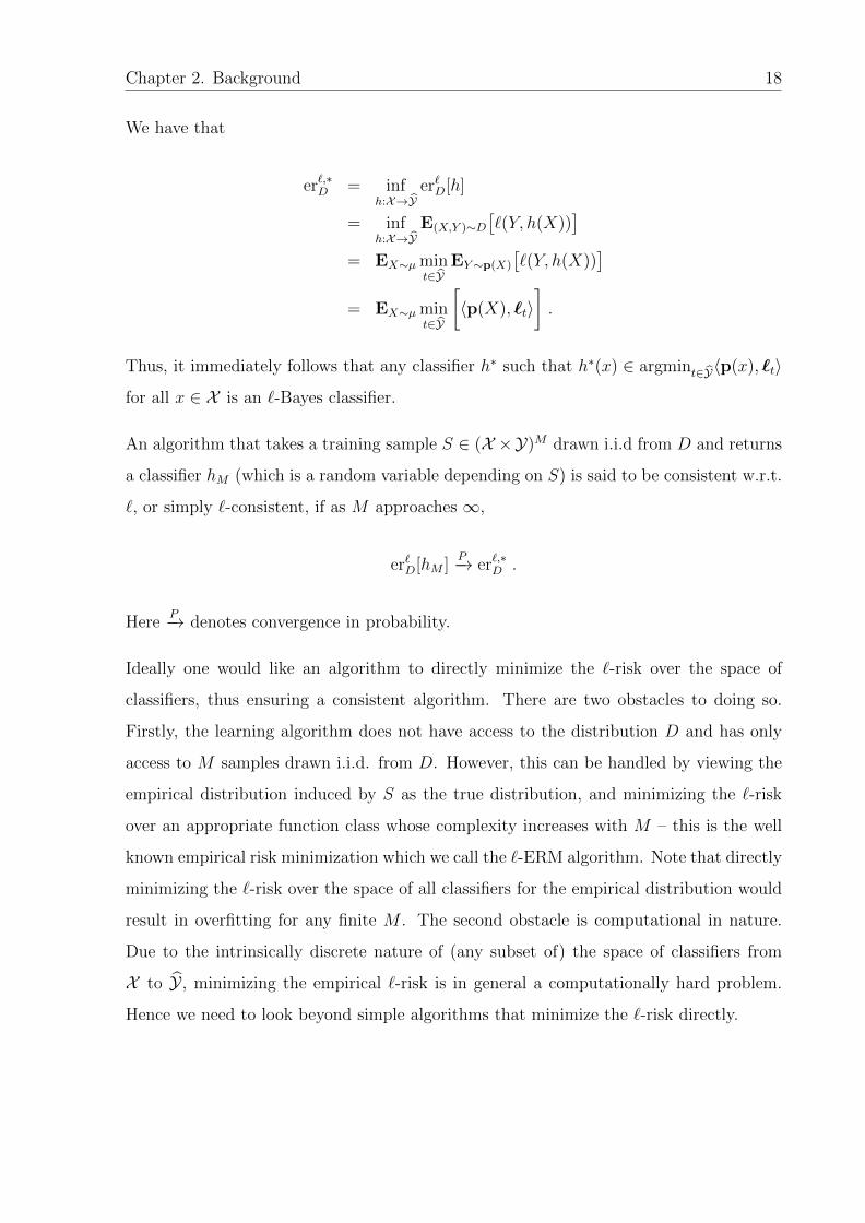
We have that
er`,∗D = infh:X→Y
er`D[h]
= infh:X→Y
E(X,Y )∼D[`(Y, h(X))
]= EX∼µ min
t∈YEY∼p(X)
[`(Y, h(X))
]= EX∼µ min
t∈Y
[〈p(X), `t〉
].
Thus, it immediately follows that any classifier h∗ such that h∗(x) ∈ argmint∈Y〈p(x), `t〉for all x ∈ X is an `-Bayes classifier.
An algorithm that takes a training sample S ∈ (X ×Y)M drawn i.i.d from D and returns
a classifier hM (which is a random variable depending on S) is said to be consistent w.r.t.
`, or simply `-consistent, if as M approaches ∞,
er`D[hM ]P−→ er`,∗D .
HereP−→ denotes convergence in probability.
Ideally one would like an algorithm to directly minimize the `-risk over the space of
classifiers, thus ensuring a consistent algorithm. There are two obstacles to doing so.
Firstly, the learning algorithm does not have access to the distribution D and has only
access to M samples drawn i.i.d. from D. However, this can be handled by viewing the
empirical distribution induced by S as the true distribution, and minimizing the `-risk
over an appropriate function class whose complexity increases with M – this is the well
known empirical risk minimization which we call the `-ERM algorithm. Note that directly
minimizing the `-risk over the space of all classifiers for the empirical distribution would
result in overfitting for any finite M . The second obstacle is computational in nature.
Due to the intrinsically discrete nature of (any subset of) the space of classifiers from
X to Y , minimizing the empirical `-risk is in general a computationally hard problem.
Hence we need to look beyond simple algorithms that minimize the `-risk directly.

Chapter 2. Background 19
2.5 Surrogate Minimizing Algorithms
A learning algorithm is formally a mapping from the set of training samples ∪∞m=1(X×Y)m
to the set of classifiers YX . A large majority of popular algorithms for multiclass learning
problems are from a special class of learning algorithms known as surrogate minimizing
algorithms, which are characterized simply by a ‘surrogate loss’. This section gives details
on such algorithms.
Let C ⊆ Rd for some integer d ∈ Z+. Let ψ : Y × C→R+ be the surrogate loss. We will
refer to d as the surrogate dimension of ψ and C as the surrogate space of ψ.
In a similar fashion to the `-risk of a classifier h : X→Y , the ψ-risk is defined for a
function f : X→C as
erψD[f ] = E(X,Y )∼D[ψ(Y, f(X))
].
The smallest possible ψ-risk is called the Bayes ψ-risk erψ,∗D .
erψ,∗D = inff :X→C
erψD[f ]
= inff :X→C
E(X,Y )∼D
[ψ(Y, f(X))
]= EX∼µ
[infu∈C〈p(X),ψ(u)〉
].
where ψ(u) = [ψ(1,u), . . . , ψ(n,u)]>. Viewing ψ as a function from C to Rn+, one can
construct two sets that are interesting and useful objects of study:
Rψ = ψ(C) ⊆ Rn+
Sψ = conv(Rψ) ⊆ Rn+ ,
where conv(R) denotes the convex hull of a set R.

Chapter 2. Background 20
Clearly, the Bayes ψ-risk can then also be written as
erψ,∗D = EX∼µ
[inf
z∈Rψ〈p(X), z〉
]= EX∼µ
[infz∈Sψ〈p(X), z〉
].
The objective of a surrogate minimizing algorithm is to find a function f : X→C, whose
ψ-risk is as small as possible. Once again we face two issues – access to the distribution
D only through the samples S, and computational difficulties. The first difficulty can be
overcome as before by using the empirical distribution, leading to the empirical surrogate
risk minimization called the ψ-ERM or simply the surrogate ERM-algorithm. The second
issue can be overcome by designing ψ to be convex. We give details of both below.
Given a training sample S = (x1, y1), . . . , (xM , yM), and class of functions FM ⊆ f :
X→C, the ψ-ERM algorithm simply returns f∗M given by
f∗M ∈ argminf∈FM1
M
M∑i=1
ψ(yi, f(xi)) .
One can show using standard uniform convergence type arguments that for an appropriate
sequence of function classes FM we have erψD[f∗M ]P−→ erψ,∗D , and such an algorithm is called
consistent w.r.t. ψ, or ψ-consistent.
Unlike the case of the `-ERM, the ψ-ERM is a continuous optimization problem, therefore
if ψ is convex in its second argument,2 with appropriate function classes Fm, the ψ-ERM
algorithm simply requires a convex optimization problem to be solved, which can be
done efficiently [10]. As an aside, we observe that the surrogate dimension d of ψ plays
a crucial component in deciding the computational difficulty of the corresponding ψ-
ERM. A surrogate minimizing algorithm using a surrogate with dimension d, requires
d functions from X to R to be learned, and hence both computational and memory
requirements increase with d.
The result of a ψ-ERM algorithm is a function f∗ from X to C. However, the learning
algorithm must return a function from X to Y . This is addressed by simply using a
2We will sometimes omit the term ‘in its second argument’ and simply say ψ is a convex surrogate.

Chapter 2. Background 21
predictor mapping pred : C→Y , and returning the classifier given by pred f∗. We give
two simple examples below.
Example 2.13 (Binary SVM for binary classification). Let Y = Y = +1,−1. The
SVM (support vector machine) algorithm is a surrogate minimizing algorithm with the
surrogate ψH : +1,−1 × R→R+ being the so called hinge loss:
ψH(1, u) = (1− u)+
ψH(−1, u) = (1 + u)+
where (a)+ = max(a, 0). As can be seen, the surrogate space of ψH is C = R, and the
‘surrogate dimension’ is d = 1. The surrogate-ERM in this case returns a function f ∗
from X to R, and the predictor pred of choice is the sign function, and thus the classifier
returned by the SVM algorithm is simply sign f ∗.
Example 2.14 (Crammer-Singer SVM for multiclass classification). Let Y = Y = [n] with
n > 2. The Crammer-Singer SVM [27] algorithm is a surrogate minimizing algorithm,
with the surrogate being a generalization of the hinge loss. The surrogate ψCS : Y ×Rn→R+ is given below.
ψCS(y,u) =n
maxi=1
(1 + ui − uy)+
As can be seen the surrogate space of ψCS is C = Rn, and the ‘surrogate dimension’ is
d = n. The surrogate-ERM in this case returns a function f∗ from X to Rn, and the
predictor pred of choice is the argmax function, and thus the classifier returned by the
algorithm is simply argmax f∗.
2.6 Calibrated Surrogates and Excess Risk Bounds
This section lays the groundwork for answering the following crucial question –
What surrogate minimizing algorithms are consistent w.r.t. a given loss function ` ?
The surrogate minimizing algorithm is characterized by the surrogate ψ and the predictor
pred and does not depend on `. Hence the surrogate ψ and predictor pred must somehow

Chapter 2. Background 22
capture the crucial qualities of the loss function `. In particular, ψ and pred must be
such that for any sequence of vector functions fM : X→C
limM→∞
erψD[fM ] = erψ,∗D implies limM→∞
er`D[pred fM ] = er`,∗D .
Such a pair (ψ, pred) is said to be calibrated w.r.t. ` or simply `-calibrated.
Sometimes it is more convenient to work with ψ and `-regrets or excess risks, than risks
directly. The `-regret, reg`D[h] of a classifier h : X→Y , and ψ-regret, regψD[f ] of a function
f : X→C are defined as
reg`D[h] = er`D[h]− infh′:X→Y
er`D[h′]
regψD[f ] = erψD[f ]− inff ′:X→C
erψD[f ′] .
Another quantity of interest is the conditional regret i.e. regret for a prediction on a
single instance given the conditional probability. The conditional `-regret, reg`p(t) and
conditional ψ-regret, regψp(u) for a conditional probability vector p ∈ ∆n, prediction
t ∈ Y and vector u ∈ C are defined as
reg`p(t) = 〈p, `t〉 − inft′∈Y〈p, `t′〉
regψp(u) = 〈p,ψ(u)〉 − infu′∈C〈p,ψ(u′)〉 .
It can be easily seen that
reg`D[h] = EX∼µ reg`p(X)(h(X))
regψD[f ] = EX∼µ regψp(X)(f(X)) .
One can show that the surrogate and predictor (ψ, pred) are `-calibrated if and only if
there exists a function ξ : R+→R+ such that ξ(0) = 0 and ξ is continuous at 0 and such
that for all f : X→Creg`D[pred f ] ≤ ξ(regψD[f ]) .

Chapter 2. Background 23
regψD[f ]
reg`D[predf ]ξ(regψD[f ])
Figure 2.2: Example illustrating the feasible `-regret and ψ-regret values for a surrogateand predictor (ψ,pred) satisfying an excess risk bound.
Such bounds are called excess risk bounds, and an illustration is given in Figure 2.2.
If a (ψ, pred) satisfies such an excess risk bound, it immediately gives a way to convert
a ψ-consistent algorithm to an `-consistent algorithm. As noted in Section 2.5, ψ-ERM
algorithms (implemented in suitable function class FM) are ψ-consistent, and if ψ is
convex are efficiently implementable. Thus, the major goal in most of this thesis will be
to construct convex calibrated surrogates for various loss matrices of interest; in fact we
will start by developing general tools that can be used to design such surrogates for any
loss matrix `.

Part I
Consistency and Calibration

Chapter 3
Conditions for Calibration
In this chapter we describe in detail the framework of calibration, and give general condi-
tions for a surrogate loss to be calibrated w.r.t. a target loss. These results significantly
generalize previous results, which have focused on specific classes of loss matrices.
3.1 Chapter Organization
We begin by defining a general notion of calibration applicable to an arbitrary multiclass
loss matrix in Section 3.2. We then define a crucial property of the loss matrix known as
trigger probability sets and a crucial property of the surrogate known as positive normals
in Section 3.3. We go on to give necessary conditions and sufficient conditions for a
surrogate to be calibrated w.r.t. a loss matrix, based on the trigger probabilities of the
loss matrix and positive normals of the surrogate in Section 3.4.
3.2 Calibration
In this section, we give a formal definition of calibration that generalizes the definitions
of Bartlett et al. [7], Tewari and Bartlett [100], Zhang [116].
25

Chapter 3. Conditions for Calibration 26
Definition 3.1 (`-calibration). Let ` : Y × Y→R+. Let ψ : Y × C→R+ and pred : C→Y.
(ψ, pred) is said to be `-calibrated if
∀p ∈ ∆n : infu∈C:pred(u)/∈argmint〈p,`t〉
〈p,ψ(u)〉 > infu∈C〈p,ψ(u)〉 .
Also, ψ is said to be `-calibrated, if there exists a pred : C→Y such that (ψ, pred) is
`-calibrated.
Another equivalent definition of calibration that is natural in some situations and gener-
alizes the definition in Tewari and Bartlett [100] is given in the Lemma below.
Lemma 3.1. Let ` : Y × Y→R+. Let ψ : Y × C→R+. Then ψ is `-calibrated iff there
exists pred′ : Sψ→Y such that
∀p ∈ ∆n : infz∈Sψ :pred′(z)/∈argmint〈p,`t〉
〈p, z〉 > infz∈Sψ〈p, z〉 .
Proof. We will show that ∃ pred : C→Y satisfying the condition in Definition 3.1 if and
only if ∃ pred′ : Sψ→Y satisfying the stated condition.
(‘if ’ direction) First, suppose ∃ pred′ : Sψ→Y such that
∀p ∈ ∆n : infz∈Sψ :pred′(z)/∈argmint〈p,`t〉
〈p, z〉 > infz∈Sψ〈p, z〉 .
Define pred : C→Y as follows:
pred(u) = pred′(ψ(u)) ∀u ∈ C .
Then for all p ∈ ∆n, we have
infu∈C:pred(u)/∈argmint〈p,`t〉
〈p,ψ(u)〉 = infz∈Rψ :pred′(z)/∈argmint〈p,`t〉
〈p, z〉
≥ infz∈Sψ :pred′(z)/∈argmint〈p,`t〉
〈p, z〉
> infz∈Sψ〈p, z〉
= infu∈C〈p,ψ(u)〉 .
Thus ψ is `-calibrated.

Chapter 3. Conditions for Calibration 27
(‘only if ’ direction) Conversely, suppose ψ is `-calibrated, so that ∃ pred : C→Y such
that
∀p ∈ ∆n : infu∈C:pred(u)/∈argmint〈p,`t〉
〈p,ψ(u)〉 > infu∈C〈p,ψ(u)〉 .
By Caratheodory’s theorem (e.g. see [8]), we have that every z ∈ Sψ can be expressed
as a convex combination of at most n + 1 points in Rψ, i.e. for every z ∈ Sψ, ∃α ∈∆n+1,u1, . . . ,un+1 ∈ C such that z =
∑n+1j=1 αjψ(uj); w.l.o.g., we can assume α1 ≥
1n+1
. For each z ∈ Sψ, arbitrarily fix a unique such convex combination, i.e. fix αz ∈∆n+1,u
z1, . . . ,u
zn+1 ∈ C with αz
1 ≥ 1n+1
such that
z =n+1∑j=1
αzjψ(uz
j ) .
Now, define pred′ : Sψ→Y as follows:
pred′(z) = pred(uz1) ∀z ∈ Sψ .
Then for any p ∈ ∆n, we have
infz∈Sψ :pred′(z)/∈argmint〈p,`t〉
〈p, z〉 = infz∈Sψ :pred(uz
1)/∈argmint〈p,`t〉
n+1∑j=1
αzj 〈p,ψ(uz
j )〉
≥ infα∈∆n+1,u1,...,un+1∈C:α1≥ 1
n+1,pred(u1)/∈argmint〈p,`t〉
n+1∑j=1
αj〈p,ψ(uj)〉
≥ infα∈∆n+1:α1≥ 1
n+1
n+1∑j=1
infuj∈C:pred(u1)/∈argmint〈p,`t〉
αj〈p,ψ(uj)〉
≥ infα1∈[ 1
n+1,1]
[α1 inf
u∈C:pred(u)/∈argmint〈p,`t〉〈p,ψ(u)〉
+(1− α1)n+1∑j=2
infu∈C〈p,ψ(u)〉
]> inf
u∈C〈p,ψ(u)〉
= infz∈Sψ〈p, z〉 .
Thus pred′ satisfies the stated condition.
Both the above definitions can be shown to be equivalent to the one mentioned in Section

Chapter 3. Conditions for Calibration 28
2.6, which essentially states that if ψ is `-calibrated, then a ψ-consistent algorithm can
be converted to an `-consistent algorithm.
Theorem 3.2. Let ` : Y × Y→R+. Let ψ : Y × C→R+ and pred : C→Y. (ψ, pred) is
`-calibrated iff for all distributions D on X × [n] and all sequences of (random) vector
functions fm : X→C, we have that
erψD[fm]P−→ erψ,∗D implies er`D[pred fm]
P−→ er`,∗D .
The proof is similar to that for the multiclass 0-1 loss given by Tewari and Bartlett [100].
Before, we give the proof, we state two lemmas; the proof of the first can be found in
Tewari and Bartlett [100], and the second follows directly from Lemma 3.1.
Lemma 3.3. The map p 7→ infz∈Sψ〈p, z〉 is continuous over ∆n.
Lemma 3.4. Let ` : Y × Y→R+. A surrogate ψ : Y ×C→Rn is `-calibrated if and only if
there exists a function pred′ : Sψ→[k] such that the following holds: for all p ∈ ∆n and all
sequences zm in Sψ such that limm→∞〈p, zm〉 = infz∈Sψ〈p, z〉, we have 〈p, `pred′(zm)〉 =
mint∈Y〈p, `t〉 for all large enough m.
Proof. (Proof of Theorem 3.2)
(‘only if ’ direction)
Let (ψ, pred) be `-calibrated. Then by Lemma 3.1, ∃ pred′ : Sψ→Y such that
∀p ∈ ∆n : infz∈Sψ :pred′(z)/∈argmint〈p,`t〉
〈p, z〉 > infz∈Sψ〈p, z〉 .
Further, for any u ∈ C we have pred(u) = pred′(ψ(u)).
Now, for each ε > 0, define
H(ε) = infp∈∆n,z∈Sψ :〈p,`pred′(z)〉−min
t∈Y 〈p,`t〉≥ε
〈p, z〉 − inf
z∈Sψ〈p, z〉
.

Chapter 3. Conditions for Calibration 29
We claim that H(ε) > 0 ∀ε > 0. Assume for the sake of contradiction that ∃ε > 0 for
which H(ε) = 0. Then there must exist a sequence (pm, zm) in ∆n × Sψ such that
〈pm, `pred′(zm)〉 −mint∈Y〈pm, `t〉 ≥ ε ∀m (3.1)
and
〈pm, zm〉 − infz∈Sψ〈pm, z〉 → 0 . (3.2)
Since pm come from a compact set, we can choose a convergent subsequence (which we still
call pm), say with limit p. Then by Lemma 3.3, we have infz∈Sψ〈pm, z〉 −→ infz∈Sψ〈p, z〉,and therefore by Equation (3.2), we get
〈pm, zm〉 −→ infz∈Sψ〈p, z〉 .
Now we show that zm is a sequence such that 〈p, zm〉 −→ infz∈Sψ〈p, z〉. Without loss of
generality, we assume that the first a coordinates of p are non-zero and the rest are zero.
Hence the first a coordinates of zm are bounded for sufficiently large m, and we have
lim supm〈p, zm〉 = lim sup
m
a∑y=1
pm,yzm,y ≤ limm→∞
〈pm, zm〉 = infz∈Sψ〈p, z〉 .
By Lemma 3.4, we therefore have 〈p, `pred′(zm)〉 = mint∈[k]〈p, `t〉 for all large enough m,
which contradicts Equation (3.1) as pm converges to p. Thus we must have H(ε) > 0 ∀ε >0. From Zhang [116], there exists a concave and non-decreasing function ξ : R+→R+
continuous at 0 with ξ(0) = 0 and satisfying the following for all u ∈ C,p ∈ ∆n.
reg`p(pred′(ψ(u))) = reg`p(pred(u)) ≤ ξ(regψp(u)
).
By Jensen’s inequality, we have for all f : X→C and all distributions D over X × Y ,
reg`p [pred f ] ≤ ξ(regψp[f ]
).
And thus any sequence of random vector functions fm such that erψD[fm]P−→ erψ,∗D satisfies
er`D[pred fm]P−→ er`,∗D .

Chapter 3. Conditions for Calibration 30
(‘if ’ direction)
Conversely, suppose ψ is not `-calibrated. Consider any pred : C→[k]. Then ∃p ∈ ∆n
such that
infu∈C:pred(u)/∈argmint〈p,`t〉
〈p,ψ(u)〉 = infu∈C〈p,ψ(u)〉 .
In particular, this means there exists a sequence of points um in C such that
pred(um) /∈ argmint〈p, `t〉 ∀m
and
〈p,ψ(um)〉 −→ infu∈C〈p,ψ(u)〉 .
Now consider a data distribution D = µ ×DY |X on X × [n], with µ being a point mass
at some x ∈ X and DY |X=x = p. Let fm : X→C be any sequence of functions satisfying
fm(x) = um ∀m. Then we have
erψD[fm] = 〈p,ψ(um)〉 ; erψ,∗D = infu∈C〈p,ψ(u)〉
and
er`D[pred fm] = 〈p, `pred(um)〉 ; er`,∗D = mint〈p, `t〉 .
This gives
erψD[fm] −→ erψ,∗D
but
er`D[pred fm] 6−→ er`,∗D .
This completes the proof.
We also have that calibration is equivalent to the existence of excess risk bounds. This is
formalized in Proposition 3.5. In some of our results, we simply show calibration via either
Definition 3.1 or Lemma 3.1. In some other cases, it is possible to derive explicit excess
risk bounds, and we do so whenever possible rather than simply showing calibration, as
it gives a better understanding of the relation between the surrogate and the true loss.
Proposition 3.5. Let ` : Y × Y→R+. Let ψ : Y × C→R+ and pred : C→Y.

Chapter 3. Conditions for Calibration 31
a. Let ξ : R+→R+ be a concave non-decreasing function such that ξ(0) = 0 and for all
distributions D and all f : X→C we have
reg`D[pred f ] ≤ ξ(regψD[f ]
).
Then (ψ, pred) is `-calibrated.
b. Let (ψ, pred) be `-calibrated. Then there exists concave non-decreasing function
ξ : R+→R+ such that ξ(0) = 0 and for all distributions D and all f : X→C we have
reg`D[pred f ] ≤ ξ(regψD[f ]
).
Proof. Part a.
Fix p ∈ ∆n. By letting D be the distribution with marginal over X concentrated at a
single point x, and such that the conditional distribution p(x) = p, we have for all u ∈ C
reg`p(pred(u)) ≤ ξ(regψp(u)
).
As the above holds for all p ∈ ∆n, we have that (ψ, pred) is `-calibrated.
Part b.
This follows from the if direction of the proof of Theorem 3.2.
3.3 Trigger Probabilities and Positive Normals
Our goal is to study conditions under which a surrogate loss ψ : Y×C→R+ is `-calibrated
for a target loss function ` : Y×Y→R+. To this end, we will now define certain properties
of both multiclass loss functions ` and multiclass surrogates ψ that will be useful in
relating the two. Specifically, we will define trigger probability sets associated with a
multiclass loss function `, and positive normal sets associated with a multiclass surrogate
Chapter 3. Conditions for Calibration 32
ψ; in Section 3.4 we will use these to obtain both necessary and sufficient conditions for
calibration.
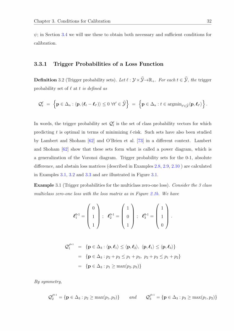
3.3.1 Trigger Probabilities of a Loss Function
Definition 3.2 (Trigger probability sets). Let ` : Y×Y→R+. For each t ∈ Y, the trigger
probability set of ` at t is defined as
Q`t =
p ∈ ∆n : 〈p, (`t − `t′)〉 ≤ 0 ∀t′ ∈ Y
=
p ∈ ∆n : t ∈ argmint′∈Y〈p, `t′〉.
In words, the trigger probability set Q`t is the set of class probability vectors for which
predicting t is optimal in terms of minimizing `-risk. Such sets have also been studied
by Lambert and Shoham [62] and O’Brien et al. [73] in a different context. Lambert
and Shoham [62] show that these sets form what is called a power diagram, which is
a generalization of the Voronoi diagram. Trigger probability sets for the 0-1, absolute
difference, and abstain loss matrices (described in Examples 2.8, 2.9, 2.10 ) are calculated
in Examples 3.1, 3.2 and 3.3 and are illustrated in Figure 3.1.
Example 3.1 (Trigger probabilities for the multiclass zero-one loss). Consider the 3 class
multiclass zero-one loss with the loss matrix as in Figure 2.1b. We have
`0-11 =
0
1
1
; `0-12 =
1
0
1
; `0-13 =
1
1
0
.
Q`0-11 = p ∈ ∆3 : 〈p, `1〉 ≤ 〈p, `2〉, 〈p, `1〉 ≤ 〈p, `3〉
= p ∈ ∆3 : p2 + p3 ≤ p1 + p3, p2 + p3 ≤ p1 + p2
= p ∈ ∆3 : p1 ≥ max(p2, p3)
By symmetry,
Q`0-12 = p ∈ ∆3 : p2 ≥ max(p1, p3) and Q`0-13 = p ∈ ∆3 : p3 ≥ max(p1, p2)

Chapter 3. Conditions for Calibration 33
See Figure 3.1a for an illustration of the trigger probabilities.
Example 3.2 (Trigger probabilities for the absolute difference loss). Consider the three
class absolute difference loss with the loss matrix as in Figure 2.1c. We have
`abs1 =
0
1
2
; `abs2 =
1
0
1
; `abs3 =
2
1
0
.
Q`abs1 = p ∈ ∆3 : 〈p, `1〉 ≤ 〈p, `2〉, 〈p, `1〉 ≤ 〈p, `3〉
= p ∈ ∆3 : p2 + 2p3 ≤ p1 + p3, p2 + 2p3 ≤ 2p1 + p2
= p ∈ ∆3 : p1 ≥ 12
By symmetry,
Q`abs3 = p ∈ ∆3 : p3 ≥ 12
Finally,
Q`abs2 = p ∈ ∆3 : 〈p, `2〉 ≤ 〈p, `1〉, 〈p, `2〉 ≤ 〈p, `3〉
= p ∈ ∆3 : p1 + p3 ≤ p2 + 2p3, p1 + p3 ≤ 2p1 + p2
= p ∈ ∆3 : p1 ≤ p2 + p3, p3 ≤ p1 + p2
See Figure 3.1b for an illustration of the trigger probabilities.
Example 3.3 (Trigger probabilities for the abstain loss). Consider the three class abstain
loss with the loss matrix as in Figure 2.1d. We have
`(?)1 =
0
1
1
; `(?)2 =
1
0
1
; `(?)3 =
1
1
0
; `(?)⊥ =
12
12
12
.

Chapter 3. Conditions for Calibration 34
(1, 0, 0) (0, 0, 1)
(0, 1, 0)
Q`1
Q`2
Q`3
(12,12, 0)
(12, 0,12)
(0, 12,12)
(13,13,
13)
(a) Zero-one loss `0-1
(1, 0, 0) (0, 0, 1)
(0, 1, 0)
Q`1
Q`2
Q`3
(12,12, 0)
(12, 0,12)
(0, 12,12)
(b) Absolute diff. loss `abs
(1, 0, 0) (0, 0, 1)
(0, 1, 0)
Q`1
Q`2
Q`4
Q`3
(12,12, 0)
(12, 0,12)
(0, 12,12)
(c) Abstain loss `(?)
Figure 3.1: Trigger probability sets for various losses, with n = 3. See Examples 3.1,3.2 and 3.3 for details.
Q`(?)1 = p ∈ ∆3 : 〈p, `1〉 ≤ 〈p, `2〉, 〈p, `1〉 ≤ 〈p, `3〉, 〈p, `1〉 ≤ 〈p, `⊥〉
= p ∈ ∆3 : p2 + p3 ≤ p1 + p3, p2 + p3 ≤ p1 + p2, p2 + p3 ≤ 12(p1 + p2 + p3)
= p ∈ ∆3 : p2 ≤ p1, p3 ≤ p1, p2 + p3 ≤ 12
= p ∈ ∆3 : p1 ≥ 12
By symmetry,
Q`(?)2 = p ∈ ∆3 : p2 ≥ 12 and Q`(?)3 = p ∈ ∆3 : p3 ≥ 1
2
Finally,
Q`(?)⊥ = p ∈ ∆3 : 〈p, `⊥〉 ≤ 〈p, `1〉, 〈p, `⊥〉 ≤ 〈p, `2〉, 〈p, `⊥〉 ≤ 〈p, `3〉
= p ∈ ∆3 : 12(p1 + p2 + p3) ≤ min(p2 + p3, p1 + p3, p1 + p2)
= p ∈ ∆3 : 12≤ 1−max(p1, p2, p3)
= p ∈ ∆3 : max(p1, p2, p3) ≤ 12
See Figure 3.1c for an illustration of the trigger probabilities.

Chapter 3. Conditions for Calibration 35
2
4
6
2
4
-5 -1 0 1 5
-5 -1 0 1 5
ψ(1, u) = (1− u)+
u
u
ψ(2, u) = (1 + u)+
(a)
z2 = (0, 2)
z4 = (2, 0)
Nψ(z1) = (1, 0)z1 = (0, 4)
z5 = (4, 0)
Nψ(z2) = conv(1, 0), (0.5, 0.5)
Nψ(z4) = conv(0.5, 0.5), (0, 1)z3 = (0.5, 1.5)
Nψ(z3) = (0.5, 0.5)
Nψ(z5) = (0, 1)
SψRψ
(0, 0)
ψ(2, .)
ψ(1, .)
(b)
Figure 3.2: The hinge loss and an illustration of its ‘image set’ Sψ along with theconstruction of positive normals at some points.
3.3.2 Positive Normals of a Surrogate
Definition 3.3 (Positive normal set at a point). Let ψ : Y × C→R+. For each point
z ∈ Sψ, the positive normal set of ψ at z is defined as1
N ψ(z) =
p ∈ ∆n : 〈p, (z− z′)〉 ≤ 0 ∀z′ ∈ Sψ
=
p ∈ ∆n : 〈p, z〉 = infz′∈Sψ〈p, z′〉
.
For any sequence of points zm in Sψ, the positive normal set of ψ at zm is defined
as2
N ψ(zm) =
p ∈ ∆n : limm→∞
〈p, zm〉 = infz′∈Sψ〈p, z′〉
.
In words, the positive normal set N ψ(z) at a point z = ψ(u) ∈ Rψ is the set of class
probability vectors for which predicting u is optimal in terms of minimizing ψ-risk. Such
sets were also studied by Tewari and Bartlett [100]. The extension to sequences of points
in Sψ is needed for technical reasons in some of our proofs. Note that for N ψ(zm) to
be well-defined, the sequence zm need not converge itself; however if the sequence zmdoes converge to some point z ∈ Sψ, then N ψ(zm) = N ψ(z).
A simple example for illustrating the positive normals is given below.
1For points z in the interior of Sψ, Nψ(z) is empty.2For sequences zm for which limm→∞〈p, zm〉 does not exist for any p, Nψ(z) is empty.

Chapter 3. Conditions for Calibration 36
Example 3.4 (Positive normals of the binary hinge loss). Let Y = Y = 1, 2. Consider
the hinge loss ψ : Y × R→R+ defined as
ψ(y, u) = 1(y = 1) · (1− u)+ + 1(y = 2) · (1 + u)+ .
A graph of the hinge loss and an illustration of the construction of positive normals is
given in Figure 3.2. In particular, setting z2 = [0, 2]> and z4 = [2, 0]> we have that
N ψ(z2) = p ∈ ∆n : p1 ≥ p2
N ψ(z4) = p ∈ ∆n : p2 ≥ p1
The trigger probabilities of loss ` can be computed directly from the definition due to
finiteness of Y , however that is not the case for the positive normals. Below, we give a
method to compute the positive normals of certain types of surrogates at a given point.
Specifically, we give an explicit method for computing N ψ(z) for convex surrogate losses
ψ operating on a convex surrogate space C ⊆ Rd, at points z = ψ(u) ∈ Rψ for which
the subdifferential ∂ψy(u) for each y ∈ [n] can be described as the convex hull of a finite
number of points in Rd; this is particularly applicable for piecewise linear surrogates.
Lemma 3.6. Let C ⊆ Rd be a convex set and let ψ : Y ×C→R+ be convex. Let z = ψ(u)
for some u ∈ C such that ∀y ∈ [n], the subdifferential of ψy at u can be written as
∂ψy(u) = conv(wy
1, . . . ,wysy)
for some sy ∈ Z+ and wy1, . . . ,w
ysy ∈ Rd. Let s =
∑ny=1 sy, and let
A =[w1
1 . . .w1s1
w21 . . .w
2s2. . . . . .wn
1 . . .wnsn
]∈ Rd×s ; B = [by,j] ∈ Rn×s ,
where by,j is 1 if the j-th column of A came from wy1, . . . ,w
ysy and 0 otherwise. Then
N ψ(z) =
p ∈ ∆n : p = Bq for some q ∈ null(A) ∩∆s
,
where null(A) ⊆ Rs denotes the null space of the matrix A.

Chapter 3. Conditions for Calibration 37
Proof. For all p ∈ Rn,
p ∈ N ψ(ψ(u)) ⇐⇒ p ∈ ∆n, 〈p,ψ(u)〉 ≤ 〈p, z′〉 ∀z′ ∈ Sψ⇐⇒ p ∈ ∆n, 〈p,ψ(u)〉 ≤ 〈p, z′〉 ∀z′ ∈ Rψ
⇐⇒ p ∈ ∆n, and the convex function φ(u′) = p>ψ(u′) =∑n
y=1 pyψy(u′)
achieves its minimum at u′ = u
⇐⇒ p ∈ ∆n, 0 ∈n∑y=1
py∂ψy(u)
⇐⇒ p ∈ ∆n, 0 =n∑y=1
py
sy∑j=1
vyjwyj for some vy ∈ ∆sy
⇐⇒ p ∈ ∆n, 0 =n∑y=1
sy∑j=1
qyjwyj for some qy = pyv
y, vy ∈ ∆sy
⇐⇒ p ∈ ∆n,Aq = 0 for some q = (p1v1, . . . , pnv
n)> ∈ ∆s, vy ∈ ∆sy
⇐⇒ p = Bq for some q ∈ null(A) ∩∆s .
In some of the steps above, we have used basic properties of convex functions that can
be found in Appendix A.
We give some examples for computation of the positive normals using Lemma 3.6 below.
Example 3.5 (Positive normal sets of ‘absolute difference’ surrogate). Let Y = [3], and
let C = R. Consider the ‘absolute difference’ surrogate ψabs : Y × R→R+ defined as
follows:
ψabs(y, u) = |u− y| ∀y ∈ [3], u ∈ R . (3.3)
Clearly, ψabs is convex (see Figure 3.3). Moreover, we have
Rψabs = ψabs(R) =
(|u− 1|, |u− 2|, |u− 3|)> : u ∈ R⊂ R3
+ .
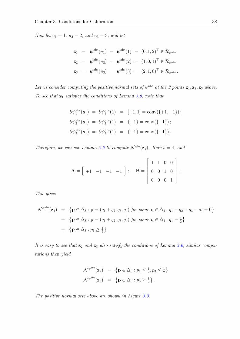
Chapter 3. Conditions for Calibration 38
Now let u1 = 1, u2 = 2, and u3 = 3, and let
z1 = ψabs(u1) = ψabs(1) = (0, 1, 2)> ∈ Rψabs
z2 = ψabs(u2) = ψabs(2) = (1, 0, 1)> ∈ Rψabs
z3 = ψabs(u3) = ψabs(3) = (2, 1, 0)> ∈ Rψabs .
Let us consider computing the positive normal sets of ψabs at the 3 points z1, z2, z3 above.
To see that z1 satisfies the conditions of Lemma 3.6, note that
∂ψabs1 (u1) = ∂ψabs
1 (1) = [−1, 1] = conv(+1,−1) ;
∂ψabs2 (u1) = ∂ψabs
2 (1) = −1 = conv(−1) ;
∂ψabs3 (u1) = ∂ψabs
3 (1) = −1 = conv(−1) .
Therefore, we can use Lemma 3.6 to compute N abs(z1). Here s = 4, and
A =[
+1 −1 −1 −1]
; B =
1 1 0 0
0 0 1 0
0 0 0 1
.
This gives
N ψabs
(z1) =p ∈ ∆3 : p = (q1 + q2, q3, q4) for some q ∈ ∆4, q1 − q2 − q3 − q4 = 0
=
p ∈ ∆3 : p = (q1 + q2, q3, q4) for some q ∈ ∆4, q1 = 1
2
=
p ∈ ∆3 : p1 ≥ 1
2
.
It is easy to see that z2 and z3 also satisfy the conditions of Lemma 3.6; similar compu-
tations then yield
N ψabs
(z2) =p ∈ ∆3 : p1 ≤ 1
2, p3 ≤ 1
2
N ψabs
(z3) =p ∈ ∆3 : p3 ≥ 1
2
.
The positive normal sets above are shown in Figure 3.3.

Chapter 3. Conditions for Calibration 39
0 0.5 1 1.5 2 2.5 3 3.5 40
0.5
1
1.5
2
2.5
3
u
ψ
1ψ
2ψ3
(a)
(1, 0, 0) (0, 0, 1)
(0, 1, 0)
N ψ(z1)
N ψ(z2)
N ψ(z3)
(b)
Figure 3.3: (a) The absolute difference surrogate ψabs : Y × R→R+ (for n = 3), and(b) its positive normal sets at 3 points zi = ψabs(ui) ∈ R3
+ (i ∈ [3]) for u1 = 1, u2 =2, u3 = 3. See Example 3.5 for details.
Example 3.6 (Positive normal sets of ε-insensitive absolute difference surrogate). Let
Y = [3], and let C = R. Let ε ∈ (0, 0.5), and consider the ε-insensitive absolute difference
surrogate ψε : Y × R→R+ defined as follows:
ψε(y, u) =(|u− y| − ε
)+
∀y ∈ [3], u ∈ R . (3.4)
For ε = 0, we have ψε = ψabs. Clearly, ψε is a convex function (see Figure 3.4). Moreover,
we have
Rψε = ψε(R) =(
(|u− 1| − ε)+, (|u− 2| − ε)+, (|u− 3| − ε)+
)>: u ∈ R
⊂ R3
+ .
For concreteness, we will take ε = 0.25 below, but similar computations hold ∀ε ∈ (0, 0.5).
Let u1 = 1 + ε = 1.25, u2 = 2− ε = 1.75, u3 = 2 + ε = 2.25, and u4 = 3− ε = 2.75, and
let
z1 = ψ0.25(u1) = ψ0.25(1.25) = (0, 0.5, 1.5)> ∈ Rψ0.25
z2 = ψ0.25(u2) = ψ0.25(1.75) = (0.5, 0, 1)> ∈ Rψ0.25
z3 = ψ0.25(u3) = ψ0.25(2.25) = (1, 0, 0.5)> ∈ Rψ0.25
z4 = ψ0.25(u4) = ψ0.25(2.75) = (1.5, 0.5, 0)> ∈ Rψ0.25 .

Chapter 3. Conditions for Calibration 40
Let us consider computing the positive normal sets of ψ0.25 at the 4 points zi (i ∈ [4])
above. To see that z1 satisfies the conditions of Lemma 3.6, note that
∂ψ0.251 (u1) = ∂ψ0.25
1 (1.25) = [0, 1] = conv(0, 1) ;
∂ψ0.252 (u1) = ∂ψ0.25
2 (1.25) = −1 = conv(−1) ;
∂ψ0.253 (u1) = ∂ψ0.25
3 (1.25) = −1 = conv(−1) .
Therefore, we can use Lemma 3.6 to compute N 0.25(z1). Here s = 4, and
A =[
0 1 −1 −1]
; B =
1 1 0 0
0 0 1 0
0 0 0 1
.
This gives
N ψ0.25
(z1) =p ∈ ∆3 : p = (q1 + q2, q3, q4) for some q ∈ ∆4, q2 − q3 − q4 = 0
=
p ∈ ∆3 : p = (q1 + q2, q3, q4) for some q ∈ ∆4, q1 + q2 ≥ q3 + q4
=
p ∈ ∆3 : p1 ≥ 1
2
.
Similarly, to see that z2 satisfies the conditions of Lemma 3.6, note that
∂ψ0.251 (u2) = ∂ψ0.25
1 (1.75) = 1 = conv(1) ;
∂ψ0.252 (u2) = ∂ψ0.25
2 (1.75) = [−1, 0] = conv(−1, 0) ;
∂ψ0.253 (u2) = ∂ψ0.25
3 (1.75) = −1 = conv(−1) .
Again, we can use Lemma 3.6 to compute N ψ0.25(z2); here s = 4, and
A =[
1 −1 0 −1]
; B =
1 0 0 0
0 1 1 0
0 0 0 1
.

Chapter 3. Conditions for Calibration 41
0 0.5 1 1.5 2 2.5 3 3.5 40
0.5
1
1.5
2
2.5
3
u
ψ
1ψ
2ψ3
(a)
(1, 0, 0) (0, 0, 1)
(0, 1, 0)
N ψ(z1)
N ψ(z2) N ψ(z3)
N ψ(z4)
(b)
Figure 3.4: (a) The ε-insensitive absolute difference surrogate ψε : Y × R→R+ forε = 0.25 (and n = 3), and (b) its positive normal sets at 4 points zi = ψε(ui) ∈ R3
+
(i ∈ [4]) for u1 = 1.25, u2 = 1.75, u3 = 2.25, u4 = 2.75. See Example 3.6 for details.
This gives
N ψ0.25
(z2) =p ∈ ∆3 : p = (q1, q2 + q3, q4) for some q ∈ ∆4, q1 − q2 − q4 = 0
=
p ∈ ∆3 : p1 ≥ p3, p1 ≤ 1
2
.
Similar computations then yield
N ψ0.25
(z3) =p ∈ ∆3 : p1 ≤ p3, p3 ≤ 1
2
N ψ0.25
(z4) =p ∈ ∆3 : p3 ≥ 1
2
.
The positive normal sets above are shown in Figure 3.4.
Example 3.7 (Positive normals of the Crammer-Singer surrogate). Consider the Crammer-
Singer surrogate introduced in Example 2.14, for n = 3. For n = 3, the Crammer-Singer
surrogate ψCS : [3]× R3→R+ is given by
ψCS(1,u) = max(1 + u2 − u1, 1 + u3 − u1, 0)
ψCS(2,u) = max(1 + u1 − u2, 1 + u3 − u2, 0)
ψCS(3,u) = max(1 + u1 − u3, 1 + u2 − u3, 0) ∀u ∈ R3 .

Chapter 3. Conditions for Calibration 42
Clearly, ψCS is convex. Let u1 = (1, 0, 0)>, u2 = (0, 1, 0)>, u3 = (0, 0, 1)>, u4 = (0, 0, 0)>,
and let
z1 = ψCS(u1) = (0, 2, 2)>
z2 = ψCS(u2) = (2, 0, 2)>
z3 = ψCS(u3) = (2, 2, 0)>
z4 = ψCS(u4) = (1, 1, 1)> .
We apply Lemma 3.6 to compute the positive normal sets of ψCS at the 4 points z1, z2, z3, z4
above. In particular, to see that z4 satisfies the conditions of Lemma 3.6, note that by
Danskin’s theorem [8], we have that
∂ψCS1 (u4) = conv
−1
+1
0
,−1
0
+1
;
∂ψCS2 (u4) = conv
+1
−1
0
,
0
−1
+1
;
∂ψCS3 (u4) = conv
+1
0
−1
,
0
+1
−1
.
We can therefore use Lemma 3.6 to compute N ψCS(z4). Here s = 6, and
A =
−1 −1 1 0 1 0
1 0 −1 −1 0 1
0 1 0 1 −1 −1
; B =
1 1 0 0 0 0
0 0 1 1 0 0
0 0 0 0 1 1
.

Chapter 3. Conditions for Calibration 43
(1, 0, 0) (0, 0, 1)
(0, 1, 0)
N ψ(z1)
N ψ(z2)
N ψ(z4)
N ψ(z3)
(12 ,12 , 0)
(12 , 0,12)
(0, 12 ,12)
Figure 3.5: Positive normal sets for the Crammer-Singer surrogate ψCS for n = 3, at 4points zi = ψCS(ui) ∈ R3
+ (i ∈ [4]) for u1 = (1, 0, 0)>, u2 = (0, 1, 0)>, u3 = (0, 0, 1)>,and u4 = (0, 0, 0)>. Details can be found in Example 3.7.
By Lemma 3.6 (and some algebra), this gives
N ψCS
(z4) =p ∈ ∆3 : p = (q1 + q2, q3 + q4, q5 + q6) for some q ∈ ∆6,
q1 + q2 = q3 + q5, q3 + q4 = q1 + q6, q5 + q6 = q2 + q4
=
p ∈ ∆3 : p1 ≤ 1
2, p2 ≤ 1
2, p3 ≤ 1
2
.
It is easy to see that z1, z2, z3 also satisfy the conditions of Lemma 3.6; similar computa-
tions then yield
N ψCS
(z1) =p ∈ ∆3 : p1 ≥ 1
2
N ψCS
(z2) =p ∈ ∆3 : p2 ≥ 1
2
N ψCS
(z3) =p ∈ ∆3 : p3 ≥ 1
2
.
An illustration of the computed positive normals is given in Figure 3.5
3.4 Conditions for Calibration
In this section, we give both necessary conditions (Section 3.4.1) and sufficient conditions
(Section 3.4.2) for a surrogate ψ to be calibrated w.r.t. an arbitrary loss function `. Both
these conditions involve the trigger probability sets of the target loss ` and the positive
normal sets of the surrogate loss ψ.

Chapter 3. Conditions for Calibration 44
(1, 0, 0) (0, 0, 1)
(0, 1, 0)
N ψ(z)
q1
q2
Q`1
Q`2
Q`3
Figure 3.6: Visual proof of Theorem 3.7.
3.4.1 Necessary Conditions for Calibration
We start by deriving necessary conditions for `-calibration of a surrogate loss ψ. Consider
what happens if for some point z ∈ Sψ, the positive normal set of ψ at z, N ψ(z), has a non-
empty intersection with the interiors of two trigger probability sets of `, sayQ`1 andQ`2 (see
Figure 3.6 for an illustration), which means ∃q1,q2 ∈ N ψ(z) with argmint∈Y〈q1, `t〉 = 1and argmint∈Y〈q2, `t〉 = 2. If ψ is `-calibrated, then by Lemma 3.1, we have ∃pred′ :
Sψ→Y such that
infz′∈Sψ :pred′(z′)6=1
〈q1, z′〉 = inf
z′∈Sψ :pred′(z′)/∈argmint〈q1,`t〉〈q1, z
′〉 > infz′∈Sψ〈q1, z
′〉 = 〈q1, z〉
infz′∈Sψ :pred′(z′)6=2
〈q2, z′〉 = inf
z′∈Sψ :pred′(z′)/∈argmint〈q2,`t〉〈q2, z
′〉 > infz′∈Sψ〈q2, z
′〉 = 〈q2, z〉 .
The first inequality above implies pred′(z) = 1; the second inequality implies pred′(z) = 2,
leading to a contradiction. This gives us the following necessary condition for `-calibration
of ψ, which requires the positive normal sets of ψ at all points z ∈ Sψ to be ‘well-behaved’
w.r.t. ` in the sense of being contained within individual trigger probability sets of ` and
generalizes the ‘admissibility’ condition used for 0-1 loss by Tewari and Bartlett [100]:
Theorem 3.7. Let ` : Y × Y→R+, and let ψ : Y × C→R+ be `-calibrated. Then for all
points z ∈ Sψ, there exists some t ∈ Y such that N ψ(z) ⊆ Q`t.
In fact, we have the following stronger necessary condition, which requires the positive
normal sets of ψ not only at all points z ∈ Sψ but also at all sequences zm in Sψ to be
contained within individual trigger probability sets of `.

Chapter 3. Conditions for Calibration 45
Theorem 3.8. Let ` : Y × Y→R+, and let ψ : Y × C→R+ be `-calibrated. Then for all
sequences zm in Sψ, there exists some t ∈ Y such that N ψ(zm) ⊆ QLt .
Proof. Assume for the sake of contradiction that there is some sequence zm in Sψ for
which N ψ(zm) is not contained in Q`t for any t ∈ Y . Then ∀t ∈ Y , ∃qt ∈ N ψ(zm)such that qt /∈ Q`t, i.e. such that t /∈ argmint′〈qt, `t′〉. Now, since ψ is `-calibrated, by
Lemma 3.4, there exists a function pred′ : Sψ→Y such that for all p ∈ N ψ(zm), we
have pred′(zm) ∈ argmint′〈p, `t′〉 for all large enough m. In particular, for p = qt, we
get pred′(zm) ∈ argmint′〈qt, `t′〉 ultimately. Since this is true for each t ∈ Y , we get
pred′(zm) ∈ ∩t∈Y argmint′〈qt, `t′〉 ultimately. However by choice of qt, this intersection is
empty, thus yielding a contradiction. This completes the proof.
Note that Theorem 3.8 includes Theorem 3.7 as a special case, since N ψ(z) = N ψ(zm)for the constant sequence zm = z ∀m. We stated Theorem 3.7 separately above since it
has a simple, direct proof that helps build intuition.
Example 3.8 (Crammer-Singer surrogate is not calibrated for 0-1 loss). Looking at the
positive normal sets of the Crammer-Singer surrogate ψCS (for n = 3) shown in Figure
3.5 and the trigger probability sets of the 0-1 loss `0-1 shown in Figure 3.1a, we see
that N ψCS(z4) is not contained in any single trigger probability set of `0-1, and therefore
applying Theorem 3.7, it is immediately clear that ψCS is not `0-1-calibrated (this was also
established previously [100, 116]).
3.4.2 Sufficient Condition for Calibration
We now give a sufficient condition for `-calibration of a surrogate loss ψ that will be helpful
in showing calibration of various surrogates. In particular, we show that for a surrogate
loss ψ to be `-calibrated, it is sufficient for the above property of positive normal sets
of ψ being contained in trigger probability sets of ` to hold for only a finite number of
points in Sψ, as long as the corresponding positive normal sets jointly cover ∆n:
Theorem 3.9. Let ` : Y × Y→R+ and ψ : Y × C→Rn+. Suppose there exist r ∈ Z+
and z1, . . . , zr ∈ Sψ such that⋃rj=1N ψ(zj) = ∆n and for each j ∈ [r], ∃t ∈ Y such that
N ψ(zj) ⊆ Q`t. Then ψ is `-calibrated.

Chapter 3. Conditions for Calibration 46
The proof uses the following technical lemma:
Lemma 3.10. Let ψ : Y × C→Rn+. Suppose there exist r ∈ N and z1, . . . , zr ∈ Rψ such
that⋃rj=1N ψ(zj) = ∆n. Then any element z ∈ Sψ can be written as z = z′+z′′ for some
z′ ∈ conv(z1, . . . , zr) and z′′ ∈ Rn+.
Proof. (Proof of Lemma 3.10)
Let S ′ = z′ + z′′ : z′ ∈ conv(z1, . . . , zr), z′′ ∈ Rn+, and suppose there exists a point
z ∈ Sψ which cannot be decomposed as claimed, i.e. such that z /∈ S ′. Then by the
Hahn-Banach theorem (e.g. see [42], corollary 3.10), there exists a hyperplane that strictly
separates z from S ′, i.e. ∃w ∈ Rn such that 〈w, z〉 < 〈w, a〉 ∀a ∈ S ′. It is easy to see
that w ∈ Rn+ (since a negative component in w would allow us to choose an element a
from S ′ with arbitrarily small 〈w, a〉).
Now consider the vector q = w/∑n
i=1 wi ∈ ∆n. Since⋃rj=1N ψ(zj) = ∆n, ∃j ∈ [r]
such that q ∈ N ψ(zj). By definition of positive normals, this gives 〈q, zj〉 ≤ 〈q, z〉, and
therefore 〈w, zj〉 ≤ 〈w, z〉. But this contradicts our construction of w (since zj ∈ S ′).Thus it must be the case that every z ∈ Sψ is also an element of S ′.
Proof. (Proof of Theorem 3.9)
We will show `-calibration of ψ via Lemma 3.1. For each j ∈ [r], let
Tj =t ∈ Y : N ψ(zj) ⊆ Q`t
;
by assumption, Tj 6= ∅ ∀j ∈ [r]. By Lemma 3.10, for every z ∈ Sψ, ∃α ∈ ∆r,u ∈ Rn+ such
that z =∑r
j=1 αjzj + u . For each z ∈ Sψ, arbitrarily fix a unique αz ∈ ∆r and uz ∈ Rn+
satisfying the above, i.e. such that
z =r∑j=1
αzjzj + uz .
Now define pred′ : Sψ→Y as
pred′(z) = mint ∈ Y : ∃j ∈ [r] such that αz
j ≥ 1r
and t ∈ Tj.

Chapter 3. Conditions for Calibration 47
We will show that ψ, along with pred′, satisfies the condition for `-calibration as in Lemma
3.1.
Fix any p ∈ ∆n. Let
Jp =j ∈ [r] : p ∈ N ψ(zj)
;
since ∆n =⋃rj=1N ψ(zj), we have Jp 6= ∅. Clearly,
∀j ∈ Jp : 〈p, zj〉 = infz∈Sψ〈p, z〉 (3.5)
∀j /∈ Jp : 〈p, zj〉 > infz∈Sψ〈p, z〉 (3.6)
Moreover, from definition of Tj, we have
∀j ∈ Jp : t ∈ Tj =⇒ p ∈ Q`t =⇒ t ∈ argmint′〈p, `t′〉 .
Thus we get
∀j ∈ Jp : Tj ⊆ argmint′〈p, `t′〉 .
Now, for any z ∈ Sψ for which pred′(z) /∈ argmint′〈p, `t′〉, we must have αzj ≥ 1
rfor
at least one j /∈ Jp (otherwise, we would have pred′(z) ∈ Tj for some j ∈ Jp, giving
pred′(z) ∈ arg mint′〈p, `t′〉, a contradiction). Thus we have
infz∈Sψ :pred′(z)/∈argmint′ 〈p,`t′ 〉
〈p, z〉 = infz∈Sψ :pred′(z)/∈argmint′ 〈p,`t′ 〉
r∑j=1
αzj 〈p, zj〉+ 〈p,uz〉
≥ infα∈∆r:αj≥ 1
rfor some j /∈Jp
r∑j=1
αj〈p, zj〉
≥ minj /∈Jp
infαj∈[ 1
r,1]αj〈p, zj〉+ (1− αj) inf
z∈Sψ〈p, z〉
> infz∈Sψ〈p, z〉 ,
where the last inequality follows from Equation (3.6). Since the above holds for all
p ∈ ∆n, by Lemma 3.1, we have that ψ is `-calibrated.
Example 3.9 (Crammer-Singer surrogate is calibrated for `(?) and `abs for n = 3). In-
specting the positive normal sets of the Crammer-Singer surrogate ψCS (for n = 3) in
Figure 3.5 and the trigger probability sets of the abstain loss `(?) in Figure 3.1c, we see

Chapter 3. Conditions for Calibration 48
that N ψCS(zi) = Q`(?)i ∀i ∈ [3], and N ψCS
(z4) = Q`(?)⊥ . Therefore by Theorem 3.9, the
Crammer-Singer surrogate ψCS is `(?)-calibrated. Similarly, looking at the trigger prob-
ability sets of the ordinal regression loss matrix `abs in Figure 3.1b and again applying
Theorem 3.9, we see that the Crammer-Singer surrogate ψCS is also `abs-calibrated. Note
however, that ψCS for larger n remains calibrated w.r.t. the abstain loss, but not w.r.t.
the absolute difference loss (Details in Chapter 7).
Example 3.10 (Absolute difference surrogate is calibrated w.r.t. `abs). Inspecting the
positive normal sets of the absolute difference surrogate ψabs (for n = 3) in Figure 3.3 and
the trigger probability sets of the absolute loss `abs in Figure 3.1b we have that N ψabs(zi) =
Q`absi ∀i ∈ [3]. Hence by Theorem 3.9, we see that ψabs is `abs-calibrated. This argument
can be easily generalized for larger n as well.
Example 3.11 (ε-insensitive absolute difference surrogate is calibrated w.r.t. `abs). Let
ε ∈ (0, 0.5). Inspecting the positive normal sets of the ε-insensitive surrogate ψε (for
n = 3) in Figure 3.4 and the trigger probability sets of the absolute loss `abs in Figure
3.1b we have that
N ψε(z1) = Q`abs1 ; N ψε(z4) = Q`abs3
N ψε(z2) ⊆ Q`abs2 ; N ψε(z3) ⊆ Q`abs2
Also clearly ∪4i=1N ψε(zi) = ∆n. Hence by Theorem 3.9, we see that ψε is `abs-calibrated.
This argument can be easily generalized for larger n as well.
Chapter 4
Convex Calibration Dimension
In this chapter we shall discuss a fundamental quantity associated with a loss matrix, that
we call the convex calibration dimension. To motivate this quantity consider the absolute
difference surrogate loss and absolute difference loss matrix as in Examples 3.5 and 3.10.
It follows that the absolute difference surrogate loss, which has a surrogate dimension
of 1, is calibrated with the absolute loss matrix for any finite n.1 This is a property of
the absolute difference loss matrix, and it is not clear if such ‘low-dimensional’ convex
calibrated surrogates exist for other loss matrices.
This immediately raises the question:
What is the smallest surrogate dimension of a convex `-calibrated surrogate ?
This is a key question as it captures all our requirements of surrogate ψ, namely, that it
be `-calibrated, convex and have a small surrogate dimension d. This question is captured
by our definition of the convex calibration dimension.
Definition 4.1 (Convex calibration dimension). Let ` : Y × Y→R+. Define the convex
calibration dimension (CC dimension) of ` as
CCdim(`) = mind ∈ Z+ : ∃ a convex set C ⊆ Rd and a convex surrogate ψ : Y × C→R+
that is `-calibrated.
1The examples discussed use n = 3, but the arguments can be generalized to any finite n easily.
49
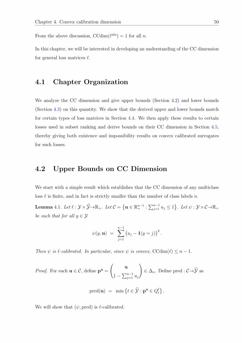
Chapter 4. Convex calibration dimension 50
From the above discussion, CCdim(`abs) = 1 for all n.
In this chapter, we will be interested in developing an understanding of the CC dimension
for general loss matrices `.
4.1 Chapter Organization
We analyze the CC dimension and give upper bounds (Section 4.2) and lower bounds
(Section 4.3) on this quantity. We show that the derived upper and lower bounds match
for certain types of loss matrices in Section 4.4. We then apply these results to certain
losses used in subset ranking and derive bounds on their CC dimension in Section 4.5,
thereby giving both existence and impossibility results on convex calibrated surrogates
for such losses.
4.2 Upper Bounds on CC Dimension
We start with a simple result which establishes that the CC dimension of any multiclass
loss ` is finite, and in fact is strictly smaller than the number of class labels n.
Lemma 4.1. Let ` : Y ×Y→R+. Let C =u ∈ Rn−1
+ :∑n−1
j=1 uj ≤ 1
. Let ψ : Y ×C→R+
be such that for all y ∈ Y
ψ(y,u) =n−1∑j=1
(uj − 1(y = j)
)2.
Then ψ is `-calibrated. In particular, since ψ is convex, CCdim(`) ≤ n− 1.
Proof. For each u ∈ C, define pu =
(u
1−∑n−1j=1 uj
)∈ ∆n. Define pred : C→Y as
pred(u) = mint ∈ Y : pu ∈ Q`
t
.
We will show that (ψ, pred) is `-calibrated.
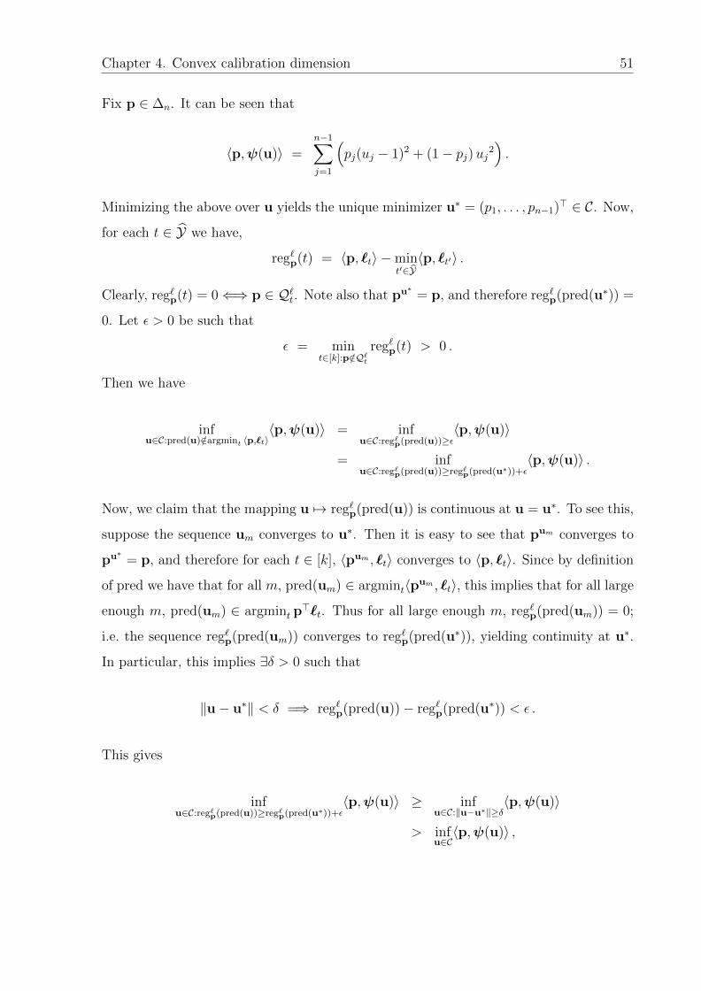
Chapter 4. Convex calibration dimension 51
Fix p ∈ ∆n. It can be seen that
〈p,ψ(u)〉 =n−1∑j=1
(pj(uj − 1)2 + (1− pj)uj2
).
Minimizing the above over u yields the unique minimizer u∗ = (p1, . . . , pn−1)> ∈ C. Now,
for each t ∈ Y we have,
reg`p(t) = 〈p, `t〉 −mint′∈Y〈p, `t′〉 .
Clearly, reg`p(t) = 0⇐⇒ p ∈ Q`t. Note also that pu∗ = p, and therefore reg`p(pred(u∗)) =
0. Let ε > 0 be such that
ε = mint∈[k]:p/∈Q`t
reg`p(t) > 0 .
Then we have
infu∈C:pred(u)/∈argmint 〈p,`t〉
〈p,ψ(u)〉 = infu∈C:reg`p(pred(u))≥ε
〈p,ψ(u)〉
= infu∈C:reg`p(pred(u))≥reg`p(pred(u∗))+ε
〈p,ψ(u)〉 .
Now, we claim that the mapping u 7→ reg`p(pred(u)) is continuous at u = u∗. To see this,
suppose the sequence um converges to u∗. Then it is easy to see that pum converges to
pu∗ = p, and therefore for each t ∈ [k], 〈pum , `t〉 converges to 〈p, `t〉. Since by definition
of pred we have that for all m, pred(um) ∈ argmint〈pum , `t〉, this implies that for all large
enough m, pred(um) ∈ argmint p>`t. Thus for all large enough m, reg`p(pred(um)) = 0;
i.e. the sequence reg`p(pred(um)) converges to reg`p(pred(u∗)), yielding continuity at u∗.
In particular, this implies ∃δ > 0 such that
‖u− u∗‖ < δ =⇒ reg`p(pred(u))− reg`p(pred(u∗)) < ε .
This gives
infu∈C:reg`p(pred(u))≥reg`p(pred(u∗))+ε
〈p,ψ(u)〉 ≥ infu∈C:‖u−u∗‖≥δ
〈p,ψ(u)〉
> infu∈C〈p,ψ(u)〉 ,

Chapter 4. Convex calibration dimension 52
where the last inequality holds since u∗ is the unique minimizer of 〈p,ψ(u)〉. The above
sequence of inequalities give us that
infu∈C:pred(u)/∈argmint 〈p,`t〉
〈p,ψ(u)〉 > infu∈C〈p,ψ(u)〉 .
Since this holds for all p ∈ ∆n, we have that ψ is `-calibrated.
It may appear surprising that the convex surrogate ψ in the above lemma, operating on a
surrogate space C ⊂ Rn−1, is `-calibrated for all multiclass losses ` on n classes. However
this makes intuitive sense, since in principle, for any multiclass problem, if one can esti-
mate the conditional probabilities of the n classes accurately (which requires estimating
n− 1 real-valued functions on X ), then one can predict a target label that minimizes the
expected loss according to these probabilities. Minimizing the above surrogate effectively
corresponds to such class probability estimation. Indeed, the above lemma can be shown
to hold for any surrogate that is a strictly proper composite multiclass loss [103].
In practice, when the number of class labels n is large (such as in a multilabel prediction
task, where n is exponential in the number of tags), the above result is not very helpful;
in such cases, it is of interest to develop algorithms operating on a surrogate prediction
space in a lower-dimensional space. Next we give a different upper bound on the CC
dimension that depends on the loss `, and for certain losses, can be significantly tighter
than the general bound above.
Theorem 4.2. Let ` : Y × Y→R+. Then
CCdim(`) ≤ affdim(L) ,
where affdim(L) denotes the dimension of the vector space parallel to the affine hull of
the column (or row) vectors of L.
Proof. Let affdim(L) = d. We will construct a convex `-calibrated surrogate loss ψ with
surrogate prediction space C ⊆ Rd.

Chapter 4. Convex calibration dimension 53
Let V ⊆ Rn denote the (d-dimensional) subspace parallel to the affine hull of the column
vectors of L, and let r ∈ Rn be the corresponding translation vector, so that
V = aff(`1, . . . , `k) + r ,
where aff(A) denotes the affine hull of the set A. Let v1, . . . ,vd ∈ V be d linearly
independent vectors in V . Let ed1, . . . , edd denote the standard basis in Rd, and define a
linear function ψ : Rd→Rn by
ψ(edj ) = vj ∀j ∈ [d] .
Then for each v ∈ V , there exists a unique vector u ∈ Rd such that ψ(u) = v. In
particular, since `t + r ∈ V for all t ∈ [k], there exist unique vectors u1, . . . ,uk ∈ Rd
such that for each t ∈ [k], ψ(ut) = `t + r. Let C = conv(u1, . . . ,uk) ⊆ Rd, and define
ψ : C→Rn+ as
ψ(u) = ψ(u)− r ∀u ∈ C .
To see that ψ(u) ∈ Rn+ ∀u ∈ C, note that for any u ∈ C, ∃α ∈ ∆k such that u =∑k
t=1 αtut, which gives ψ(u) = ψ(u)−r =(∑k
t=1 αtψ(ut))−r =
(∑kt=1 αt(`t+r)
)−r =∑k
t=1 αt`t (and `t ∈ Rn+ ∀t ∈ [k]).
Let ψ : [n] × C→R+ be the surrogate associated with ψ. The surrogate ψ is clearly
convex. To show ψ is `-calibrated, we will use Theorem 3.9. Specifically, consider the k
points zt = ψ(ut) = `t ∈ Rψ for t ∈ [k]. By definition of ψ, we have Sψ = conv(ψ(C)) =
conv(`1, . . . , `k); from the definitions of positive normals and trigger probabilities, it
then follows that N ψ(zt) = N ψ(`t) = Q`t for all t ∈ [k]. Thus by Theorem 3.9, ψ is
`-calibrated.
Since affdim(L) is equal to either rank(L) or rank(L)− 1, this immediately gives us the
following corollary:
Corollary 4.3. Let ` : Y × Y→R+. Then CCdim(`) ≤ rank(L).

Chapter 4. Convex calibration dimension 54
Example 4.1 (CC dimension of Hamming loss). Let r ∈ N. Let Y = Y = 0, 1r. The
Hamming loss `Ham as defined in Example 2.11 can be expressed as
`Ham(y, t) =r∑i=1
1(yi 6= ti)
=r∑i=1
yi + ti − 2yiti
=r∑i=1
ti +r∑i=1
yi(1− 2ti) .
Thus the loss matrix for the hamming loss can be expressed as a sum of r rank-1 ma-
trices, and a matrix that depends only on the column (or t in this case). Clearly, the
affine dimension of such a matrix is at most r. Hence we have from Theorem 4.2,
that CCdim(`Ham) ≤ r, which is significantly better than the bound of 2r − 1 got from
Lemma 4.1.
Theorem 4.2 guarantees the existence of a convex `-calibrated surrogate with dimension
affdim(L). Indeed, the proof of Theorem 4.2 constructs such a surrogate. However, this
constructed surrogate is undesirable, as the surrogate space C is an awkward subset of
Raffdim(L) and the predictor mapping pred is not given explicitly. We rectify both these
shortcomings in Chapter 5, and give many other example loss matrices used in ranking
and multi-label prediction where the size of the loss matrix is exponential in its rank.
4.3 Lower Bounds on CC Dimension
In this section we give a lower bound on the CC dimension of a loss ` and illustrate this
by using it to calculate the CC dimension of the 0-1 loss. We will need the following
definition:
Definition 4.2. The feasible subspace dimension of a convex set Q ⊆ Rn at a point
p ∈ Q, denoted by νQ(p), is defined as the dimension of the subspace FQ(p)∩ (−FQ(p)),
where FQ(p) is the cone of feasible directions of Q at p.2
2For a set Q ⊆ Rn and point p ∈ Q, the cone of feasible directions of Q at p is defined asFQ(p) = v ∈ Rn : ∃ε0 > 0 such that p + εv ∈ Q ∀ε ∈ (0, ε0).

Chapter 4. Convex calibration dimension 55
Q
p1
p2
p3
(a) The convex set Q
FQ(p1) −FQ(p1)
(b) dim(FQ(p1) ∩ (−FQ(p1))) = 2
FQ(p2) −FQ(p2)
(c) dim(FQ(p2) ∩ (−FQ(p2))) = 1
FQ(p3)
−FQ(p3)
(d) dim(FQ(p3) ∩ (−FQ(p3))) = 0
Figure 4.1: Illustration of feasible subspace dimension νQ(p) at various points p1,p2,p3
for some 2-dimensional set Q. Clearly νQ(p1) = 2, νQ(p2) = 1, νQ(p3) = 0.
Essentially, the feasible subspace dimension of a convex set Q at a point p, is simply the
dimension of the smallest face of Q containing p. An illustration of the feasible subspace
dimension is given in Figure 4.1.
Both the proof of the lower bound and its applications make use of the following lemma,
which gives a method to calculate the feasible subspace dimension for certain convex sets
Q and points p ∈ Q:
Lemma 4.4. Let Q =q ∈ Rn : A1q ≤ b1,A2q ≤ b2,A3q = b3
. Let p ∈ Q be
such that A1p = b1, A2p < b2. Then νQ(p) = nullity
([A1
A3
]), where nullity(A) =
dim(null(A)) is the dimension of the null space of A.

Chapter 4. Convex calibration dimension 56
Proof. We will show that FQ(p) ∩ (−FQ(p)) = null
([A1
A3
]), from which the lemma
follows.
First, let v ∈ null
([A1
A3
]). Then for ε > 0, we have
A1(p + εv) = A1p + εA1v = A1p + 0 = b1
A2(p + εv) < b2 for small enough ε, since A2p < b2
A3(p + εv) = A3p + εA3v = A3p + 0 = b3 .
Thus v ∈ FQ(p). Similarly, we can show −v ∈ FQ(p). Thus v ∈ FQ(p) ∩ (−FQ(p)),
giving null
([A1
A3
])⊆ FQ(p) ∩ (−FQ(p)).
Now let v ∈ FQ(p)∩(−FQ(p)). Then for small enough ε > 0, we have both A1(p+εv) ≤b1 and A1(p−εv) ≤ b1. Since A1p = b1, this gives A1v = 0. Similarly, for small enough
ε > 0, we have A3(p + εv) = b3; since A3p = b3, this gives A3v = 0. Thus
[A1
A3
]v = 0,
giving FQ(p) ∩ (−FQ(p)) ⊆ null
([A1
A3
]).
The following gives a lower bound on the CC dimension of a loss ` in terms of the feasible
subspace dimension of the trigger probability sets Q`t at points p ∈ Q`t:
Theorem 4.5. Let ` : Y × Y→R+. Let p ∈ ∆n and t ∈ argmint′〈p, `t′〉 (equivalently, let
p ∈ Q`t). Then
CCdim(`) ≥ ‖p‖0 − νQ`t(p)− 1 .
The proof will require the lemma below, which relates the feasible subspace dimensions of
different trigger probability sets at points in their intersection; we will also make critical
use of the notion of ε-subdifferentials of convex functions [8], the main properties of which
are given in Appendix A.

Chapter 4. Convex calibration dimension 57
Lemma 4.6. Let ` : Y×Y→R+. Let p ∈ relint(∆n).3 Then for any t1, t2 ∈ arg mint′〈p, `t′〉(i.e. such that p ∈ Q`t1 ∩Q`t2),
νQ`t1(p) = νQ`t2
(p) .
Proof. (Proof of Lemma 4.6)
Let t1, t2 ∈ arg mint′〈p, `t′〉 (i.e. p ∈ Q`t1 ∩Q`t2). Now
Q`t1 =q ∈ Rn : −q ≤ 0,1>nq = 1, (`t1 − `t)>q ≤ 0 ∀t ∈ Y
,
where 1n is the n-dimensional all ones vector. Moreover, we have −p < 0, and p>(`t1 −`t) = 0 iff p ∈ Q`t. Let
t ∈ Y : p ∈ Q`t
=t1, . . . , tr
for some r ∈ [k]. Then by
Lemma 4.4, we have
νQ`t1= nullity(A1) ,
where A1 ∈ R(r+1)×n is a matrix containing r rows of the form (`t1 − `tj)>, j ∈ [r] and
the all ones row. Similarly, we get
νQ`t2= nullity(A2) ,
where A2 ∈ R(r+1)×n is a matrix containing r rows of the form (`t2−`tj)>, j ∈ [r] and the
all ones row. It can be seen that the subspaces spanned by the first r rows of A1 and A2
are both equal to the subspace parallel to the affine space containing `t1 , . . . , `tr . Thus
both A1 and A2 have the same row space and hence the same null space and nullity, and
therefore νQ`t1(p) = νQ`t2
(p).
Proof. (Proof of Theorem 4.5)
Let d ∈ Z+ be such that there exists a convex set C ⊆ Rd and a convex surrogate loss
ψ : Y ×C→R+ such that ψ is `-calibrated. We will show that d ≥ ‖p‖0− νQ`t(p)− 1. We
consider two cases:
Case 1: p ∈ relint(∆n).
3relint(A) is the relative interior of the set A.

Chapter 4. Convex calibration dimension 58
In this case ‖p‖0 = n. We will show that there exist H ⊆ ∆n and t0 ∈ Y satisfying
the following two conditions:
(a) νH(p) = n− d− 1 ; and
(b) H ⊆ Q`t0 .
This will give
νQ`t0(p) ≥ νH(p) = n− d− 1 .
Clearly, condition (b) above implies p ∈ Q`t0 . By Lemma 4.6, we then have that
νQ`t(p) = νQ`t0(p) ≥ n− d− 1 ,
thus proving the claim.
The procedure to construct H and t0 follows.
Let um be a sequence in C such that
〈p,ψ(um)〉 = infu∈C〈p,ψ(u)〉+ εm .
for some sequence εm ↓ 0. Denote the sequence ψ(um) in Sψ by zm. Note
that the sequence zm is bounded.
Hence,
0 ∈ ∂εm(〈p,ψ(um)〉) ⊆ ∂εm(p1ψ1(um)) + . . .+ ∂εm(pnψn(um)) .
Thus, for all y ∈ [n] there exists a wm,y ∈ ∂(εm/py)(ψy(um)) such that
∑y∈[n]
pywm,y = Amp = 0 ,
where
Am =[wm,1 . . .wm,n
]∈ Rd×n ..

Chapter 4. Convex calibration dimension 59
Now, define the set Hm ⊆ ∆n as
Hm = q ∈ ∆n : Amq = 0 = q ∈ Rn : Amq = 0,1>nq = 1,q ≥ 0 .
Note that p ∈ Hm for all m.
Let qm ∈ Hm, then
0 =∑y∈[n]
qm,ywm,y
∈∑y∈[n]
qm,y∂(εm/py)(ψy(um))
=∑y∈[n]
∂(εmqm,y/py)(qm,yψy(um))
⊆∑y∈[n]
∂ε∗m(qm,yψy(um))
⊆ ∂nε∗m(〈qm,ψ(um)〉) ,
where ε∗m = εm maxy1py
.
Therefore for all m ∈ N, we have
〈qm, zm〉 = 〈qm,ψ(um)〉 ≤ infu∈Rd〈qm,ψ(u)〉+ nε∗m = inf
z∈Sψ〈qm, z〉+ nε∗m . (4.1)
As m approaches ∞, the above inequality becomes
limm→∞
〈qm, zm〉 ≤ limm→∞
infz∈Sψ〈qm, z〉 . (4.2)
Let the sequence qm have a limit q, we then have the following by virtue of zm
being a bounded sequence
limm→∞
〈qm, zm〉 = limm→∞
〈(qm − q), zm〉+ limm→∞
〈q, zm〉 = limm→∞
〈q, zm〉 . (4.3)
Also, from Lemma 3.3, the mapping p 7→ infz∈Sψ〈p, z〉 is continuous over its domain.
Thus,
limm→∞
infz∈Sψ〈qm, z〉 = inf
z∈Sψ〈q, z〉 . (4.4)

Chapter 4. Convex calibration dimension 60
Putting Equations (4.2), (4.3) and (4.4) together, we get
limm→∞
〈q, zm〉 = infz∈Sψ〈q, z〉 . (4.5)
Thus we have that, any q ∈ ∆n which is a limit of any sequence of points qmwith qm ∈ Hm, is such that q ∈ N ψ(zm).
We will construct a set H all of whose elements can be expressed as a limit of some
sequence of points qm with qm ∈ Hm. It can be seen that such a set will satisfy
the condition (b) as stated in the beginning of the proof, i.e. H ⊆ Q`t0 , because
H ⊆ N ψ(zm) and by Theorem 3.8 we have that
N ψ(zm) ⊆ Q`t0 for some t0 ∈ Y .
If we can ensure that such a set H also satisfies condition (a), i.e. νH(p) = n−d−1,
we are done. The construction of H follows.
Let xm,1, . . . ,xm,n−d−1 be an orthonormal set of vectors in Rn, such that
Hm ⊇ (span(xm,1, . . . ,xm,n−d−1) + p) ∩∆n .
Such a sequence always exists by the construction of Hm. As xm,1, . . . ,xm,n−d−1take values in a bounded subset of Rn(n−d−1) for all m ∈ N, there is a subsequence
converging to some x1, . . . ,xn−d−1. We will restrict our attention to this sub-
sequence. It can be seen that x1, . . . ,xn−d−1 also forms n − d − 1 orthonormal
vectors. Let
H = (span(x1, . . . ,xn−d−1) + p) ∩∆n .
It can be seen that this set H ⊆ ∆n is such that every element q ∈ H can be
expressed as a limit of some sequence qm, with qm ∈ Hm. Also, as p ∈ relint(∆n),
it follows directly from the definition of the feasible subspace dimension ν, that
νH(p) = n− d− 1.
Case 2: p /∈ relint(∆n).

Chapter 4. Convex calibration dimension 61
For each b ∈ 0, 1n \ 0, define
Pb =q ∈ ∆n : qy > 0⇐⇒ by = 1
.
Clearly, the set Pb : b ∈ 0, 1n \ 0 forms a partition of ∆n. Moreover, for
b = 1n (the all-ones vector), we have
P1n =q ∈ ∆n : qy > 0 ∀y ∈ [n]
= relint(∆n) .
Therefore we have p ∈ Pb for some b ∈ 0, 1n \ 0,1n, with ‖p‖0 = ‖b‖0. Now,
define ψb : C→R‖b‖0+ , Lb ∈ R‖b‖0×k+ , and pb ∈ ∆‖b‖0 as projections of ψ, L and p
onto the ‖b‖0 coordinates y : by = 1, so that ψb(u) contains the elements of ψ(u)
corresponding to coordinates y : by = 1, the columns `bt of Lb contain the elements of
the columns `t of L corresponding to the same coordinates y : by = 1, and similarly,
pb contains the strictly positive elements of p. Since ψ is `-calibrated, we have
that ψb is `b-calibrated. Moreover, by construction, we have pb ∈ relint(∆‖b‖0).
Therefore by Case 1 above, we have
d ≥ ‖b‖0 − νQ`bt (pb)− 1 .
The claim follows since νQ`bt(pb) ≤ νQ`t(p).
The above lower bound allows us to calculate precisely the CC dimension of the 0-1 loss:
Example 4.2 (CC dimension of 0-1 loss). Let Y = Y = [n], and consider the 0-1 loss
`0-1 : Y × Y→R+ as defined in Example 2.8. Let Q0-1t denote the trigger probability set
associated with t ∈ Y. Take p = ( 1n, . . . , 1
n)> ∈ ∆n. Then p ∈ Q0-1
t for all t ∈ Y (see
Figure 3.1a); in particular, we have p ∈ Q0-11 . Now Q0-1
1 can be written as
Q0-11 =
q ∈ ∆n : q1 ≥ qy ∀y ∈ 2, . . . , n
=
q ∈ Rn :
[−1n−1 In−1
]q ≤ 0,−q ≤ 0,1>nq = 1 ,

Chapter 4. Convex calibration dimension 62
where and In−1 denotes the (n − 1) × (n − 1) identity matrix. Moreover, we have[−1n−1 In−1
]p = 0, −p < 0. Therefore, by Lemma 4.4, we have
νQ0-11
(p) = nullity
−1n−1 In−1
1>n
= nullity
−1 1 0 . . . 0
−1 0 1 . . . 0...
−1 0 0 . . . 1
1 1 1 . . . 1
= 0 .
Moreover, ‖p‖0 = n. Thus by Theorem 4.5, we have CCdim(`0-1) ≥ n − 1. Combined
with the upper bound of Lemma 4.1, this gives CCdim(`0-1) = n− 1.
4.4 Tightness of Bounds
The upper and lower bounds above are not necessarily tight in general. For example, for
the n-class absolute difference loss of Example 2.9 used in ordinal regression, we know that
CCdim(`abs) = 1; however the upper bound of Theorem 4.2 only gives CCdim(`abs) ≤n − 1. Similarly, for the n-class abstain loss of Example 2.10, it can be shown that
CCdim(`(?)) ≤ dlog2(n)e (in fact we conjecture CCdim(`(?)) = dlog2(n)e), whereas the
upper bound of Theorem 4.2 gives CCdim(`(?)) ≤ n, and the lower bound of Theorem 4.5
yields only CCdim(`(?)) ≥ 1. However, as we show below, for certain losses `, the bounds
of Theorems 4.2 and 4.5 are in fact tight (upto an additive constant of 1).
Theorem 4.7. Let ` : Y×Y→R+. If ∃p ∈ relint(∆n), c ∈ R+ such that 〈p, `t〉 = c ∀t ∈ Y,
then
CCdim(`) ≥ affdim(L)− 1 .
Proof. Since 〈p, `t〉 = c ∀t ∈ Y , we have p ∈ Q`t ∀t ∈ Y . In particular, we have p ∈ Q`1.
Now
Q`1 =
q ∈ Rn :
(`2 − `1)>
...
(`k − `1)>
q ≥ 0,−q ≤ 0,1>nq = 1
.
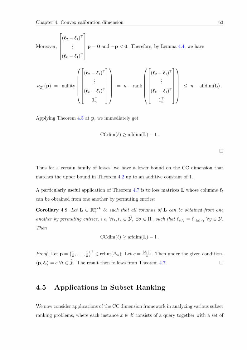
Chapter 4. Convex calibration dimension 63
Moreover,
(`2 − `1)>
...
(`k − `1)>
p = 0 and −p < 0. Therefore, by Lemma 4.4, we have
νQ`1(p) = nullity
(`2 − `1)>
...
(`k − `1)>
1>n
= n− rank
(`2 − `1)>
...
(`k − `1)>
1>n
≤ n− affdim(L) .
Applying Theorem 4.5 at p, we immediately get
CCdim(`) ≥ affdim(L)− 1 .
Thus for a certain family of losses, we have a lower bound on the CC dimension that
matches the upper bound in Theorem 4.2 up to an additive constant of 1.
A particularly useful application of Theorem 4.7 is to loss matrices L whose columns `t
can be obtained from one another by permuting entries:
Corollary 4.8. Let L ∈ Rn×k+ be such that all columns of L can be obtained from one
another by permuting entries, i.e. ∀t1, t2 ∈ Y , ∃σ ∈ Πn such that `y,t2 = `σ(y),t1 ∀y ∈ Y.
Then
CCdim(`) ≥ affdim(L)− 1 .
Proof. Let p =(
1n, . . . , 1
n
)> ∈ relint(∆n). Let c = ‖`1‖1n
. Then under the given condition,
〈p, `t〉 = c ∀t ∈ Y . The result then follows from Theorem 4.7.
4.5 Applications in Subset Ranking
We now consider applications of the CC dimension framework in analyzing various subset
ranking problems, where each instance x ∈ X consists of a query together with a set of
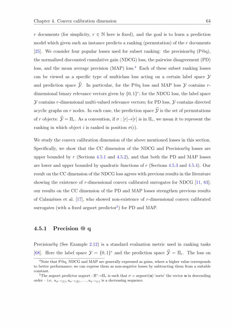
Chapter 4. Convex calibration dimension 64
r documents (for simplicity, r ∈ N here is fixed), and the goal is to learn a prediction
model which given such an instance predicts a ranking (permutation) of the r documents
[25]. We consider four popular losses used for subset ranking: the precision@q (P@q),
the normalized discounted cumulative gain (NDCG) loss, the pairwise disagreement (PD)
loss, and the mean average precision (MAP) loss.4 Each of these subset ranking losses
can be viewed as a specific type of multiclass loss acting on a certain label space Yand prediction space Y . In particular, for the P@q loss and MAP loss Y contains r-
dimensional binary relevance vectors given by 0, 1r; for the NDCG loss, the label space
Y contains r-dimensional multi-valued relevance vectors; for PD loss, Y contains directed
acyclic graphs on r nodes. In each case, the prediction space Y is the set of permutations
of r objects: Y = Πr. As a convention, if σ : [r]→[r] is in Πr, we mean it to represent the
ranking in which object i is ranked in position σ(i).
We study the convex calibration dimension of the above mentioned losses in this section.
Specifically, we show that the CC dimension of the NDCG and Precision@q losses are
upper bounded by r (Sections 4.5.1 and 4.5.2), and that both the PD and MAP losses
are lower and upper bounded by quadratic functions of r (Sections 4.5.3 and 4.5.4). Our
result on the CC dimension of the NDCG loss agrees with previous results in the literature
showing the existence of r-dimensional convex calibrated surrogates for NDCG [11, 83];
our results on the CC dimension of the PD and MAP losses strengthen previous results
of Calauzenes et al. [17], who showed non-existence of r-dimensional convex calibrated
surrogates (with a fixed argsort predictor5) for PD and MAP.
4.5.1 Precision @ q
Precision@q (See Example 2.12) is a standard evaluation metric used in ranking tasks
[68]. Here the label space Y = 0, 1r and the prediction space Y = Πr. The loss on
4Note that P@q, NDCG and MAP are generally expressed as gains, where a higher value correspondsto better performance; we can express them as non-negative losses by subtracting them from a suitableconstant.
5The argsort predictor argsort : Rr→Πr is such that σ = argsort(u) ‘sorts’ the vector u in descendingorder – i.e. uσ−1(1), uσ−1(2), . . . , uσ−1(r) is a decreasing sequence.

Chapter 4. Convex calibration dimension 65
predicting a permutation σ ∈ Πr when the true label is y ∈ 0, 1r is given by
`P@q(y, σ) = 1− 1
q
q∑i=1
yσ−1(i) .
Clearly, affdim(LP@q) ≤ r, and therefore by Theorem 4.2, we have
CCdim(`P@q) ≤ r .
Thus, there exists r-dimensional convex `P@q-calibrated surrogates and we give such sur-
rogates along with predictors in Chapter 5.
4.5.2 Normalized Discounted Cumulative Gain (NDCG)
The NDCG loss is widely used in information retrieval applications [51]. Here Y is the
set of r-dimensional relevance vectors with (say) s relevance levels, Y = 0, 1, . . . , s−1r,and Y is the set of permutations of r objects, Y = Πr (thus, here n = |Y| = sr and
k = |Y| = r!). The loss on predicting a permutation σ ∈ Πr when the true label is
y ∈ 0, 1, . . . , s− 1r is given by
`NDCG(y, σ) = 1− 1
z(y)
r∑i=1
2yi − 1
log2(σ(i) + 1),
where z(y) is a normalizer that ensures the loss is non-negative and z(y) depends only on
y. The NDCG loss can therefore be viewed as a multiclass loss matrix LNDCG ∈ Rsr×r!+ .
Clearly, affdim(LNDCG) ≤ r, and therefore by Theorem 4.2, we have
CCdim(`NDCG) ≤ r .
Indeed, previous results in the literature [11, 83] have shown the existence of r-dimensional
convex calibrated surrogates for NDCG, we also give such surrogates along with predictors
in Chapter 5.

Chapter 4. Convex calibration dimension 66
4.5.3 Pairwise Disagreement (PD)
The pairwise disagreement loss is a natural loss for ranking based on how many pairs
of documents are ordered incorrectly, and is one of the prevalent methods for evaluating
rankings [24, 28, 37]. In its most general version, the label space Y is the set of all directed
acyclic graphs (DAGs) on r vertices, which we shall denote as Gr; for each directed edge
(i, j) in a graph G ∈ Gr associated with an instance x ∈ X , the i-th document in the
document set in x is preferred over the j-th document. The prediction space Y is again
the set of permutations of r objects, Y = Πr. The loss on predicting a permutation
σ ∈ Πr when the true label is G ∈ Gr is given by
`PD(G, σ) =∑
(i,j)∈G1(σ(i) > σ(j)
)=
r∑i=1
r∑j=1
1((i, j) ∈ G
)· 1(σ(i) > σ(j)
)=
r∑i=1
i−1∑j=1
1((i, j) ∈ G
)· 1(σ(i) > σ(j)
)+ 1((j, i) ∈ G
)·(
1− 1(σ(i) > σ(j)
))=
r∑i=1
i−1∑j=1
(1((i, j) ∈ G
)− 1((j, i) ∈ G
))· 1(σ(i) > σ(j)
)+
r∑i=1
i−1∑j=1
1((j, i) ∈ G
).
The PD loss can be viewed as a multiclass loss matrix LPD ∈ R|Gr|×r!+ . Note that the
second term in the sum above depends only the label G; removing this term amounts
to simply subtracting a fixed vector from each column of the loss matrix and hence LPD
clearly is such that
affdim(LPD) ≤ r(r − 1)
2.
Therefore, by Theorem 4.2, we have
CCdim(`PD) ≤ r(r − 1)
2.
In fact one can also give tight lower bounds for CCdim(`PD) using the following proposi-
tion.
Proposition 4.9. rank(LPD) ≥ r(r−1)2
.

Chapter 4. Convex calibration dimension 67
Proof. Consider the r(r−1)2×r! sub-matrix of the loss matrix LPD with rows corresponding
to graphs consisting of single directed edges (i, j), with i < j. Let us denote this matrix
by LPD and its entry corresponding to the graph with a single directed edge (i, j), and
permutation σ as ((i, j), σ). We show that the rank of LPD is at least r(r−1)2
, by showing
that the rows of LPD are linearly independent.
To see this, assume the contrary, that one of the rows of L (say the row corresponding to
the graph (a, b) with a, b ∈ [r], a < b), can be written as linear combination of the other
rows as follows.
((a, b), σ) =r∑i=1
r∑j=i+1
c(i,j)((i, j), σ) ∀σ ∈ Πr , (4.6)
for some coefficients c(i,j) ∈ R, with c(a,b) = 0.
Consider 2 permutations σ1, σ2 ∈ Πr, which are such that
σ1(a) = σ2(b), σ1(b) = σ2(a), and σ1(i) = σ2(i),∀i ∈ [r] \ a, b .
It can be easily seen that for the columns corresponding to these 2 permutations all entries
on rows other than row (a, b) are identical, but differ on row (a, b), i.e.
((i, j), σ1
)= ((i, j), σ2
), ∀i, j ∈ [r], i < j, (i, j) 6= (a, b) , (4.7)((a, b), σ1
)6= ((a, b), σ2
). (4.8)
Applying Equation (4.6) for σ = σ1 and σ = σ2 along with Equation (4.7), we get
((a, b), σ1
)= ((a, b), σ2
),
which contradicts Equation (4.8). Thus, we have that, the rows of L are linearly inde-
pendent. This give us
rank(LPD) ≥ r(r − 1)
2.

Chapter 4. Convex calibration dimension 68
Moreover, it is easy to see that the columns of LPD can all be obtained from one another
by permuting entries. Therefore, by Corollary 4.8, we also have
CCdim(`PD) ≥ r(r − 1)
2− 2 .
This strengthens previous results of Duchi et al. [34] and Calauzenes et al. [17]. In
particular, Duchi et al. [34] showed that certain popular r-dimensional convex surrogates
are not calibrated for the PD loss, and conjectured that such convex calibrated surrogates
(in r dimensions) do not exist; Calauzenes et al. [17] showed that indeed there do not
exist any r-dimensional convex surrogates along with argsort as the predictor that are
calibrated w.r.t. the PD loss. The above result allows us to go further and conclude that
in fact, one cannot design convex calibrated surrogates for the PD loss in any prediction
space of less than r(r−1)2− 2 dimensions (regardless of the predictor used).
Many popular ranking algorithms like RankBoost [37], RankNet [13], LambdaRank [14]
and RankSVM [48, 54], are surrogate minimizing algorithms that minimize a r-dimensional
convex surrogate and simply use argsort to predict a ranking from the r-dimensional score
vector. These negative results immediately tell us that none of these surrogates are cal-
ibrated w.r.t. the PD loss. Hence it suggests to us that if the PD loss is the loss of
interest, and no distributional assumptions can be made, then one needs completely new
surrogates (algorithms) to achieve consistency.
On the other hand, the upper bound also indicates that there do exist convex calibrated
surrogates for the PD loss in r(r−1)2
dimensions; we give such surrogates along with pre-
dictors in Chapter 5.
4.5.4 Mean Average Precision (MAP)
The Mean Average Precision is another widely used evaluation metric in ranking [68].
Here the label space Y is the set of all (non-zero) r-dimensional binary relevance vectors,
Y = 0, 1r \ 0, and the prediction space Y is again the set of permutations of r
objects, Y = Πr. The loss on predicting a permutation σ ∈ Πr when the true label is

Chapter 4. Convex calibration dimension 69
y ∈ 0, 1r \ 0 is given by
`MAP(y, σ) = 1− 1
‖y‖1
∑i:yi=1
1
σ(i)
σ(i)∑j=1
yσ−1(j)
= 1− 1
‖y‖1
r∑i=1
i∑j=1
yσ−1(i) yσ−1(j)
i
= 1− 1
‖y‖1
r∑i=1
i∑j=1
yi yjmax(σ(i), σ(j))
(4.9)
Thus the MAP loss can be viewed as a multiclass loss matrix LMAP ∈ R(2r−1)×r!+ . Clearly,
affdim(LMAP) ≤ r(r + 1)
2,
and therefore by Theorem 4.2, we have
CCdim(`MAP) ≤ r(r + 1)
2.
One can also show the following lower bound on the rank of LMAP:
Proposition 4.10. rank(LMAP) ≥ r(r−1)2− 2.
Proof. By Equation (4.9) the (2r − 1)× r! loss matrix LMAP = Lr can be written as
Lr = 12r−11>r! −ArBr
where for any a ∈ N, 1a ∈ Ra is the all ones vector, Ar is a (2r − 1)× r(r+1)2
matrix and
Br is a r(r+1)2× r! matrix.
Let us denote the rows of Ar by labellings y ∈ Y = 0, 1r \ 0r and columns by pairs
(i, j) such that i, j ∈ [r], i ≤ j. Similarly, denote the rows of Br by pairs (i, j) such that
i, j ∈ [r], i ≤ j and columns by permutations σ ∈ Y = Πr.
The entries of Ar are given as
Ar(y, (i, j)) =1∑rγ=1 yγ
yiyj .

Chapter 4. Convex calibration dimension 70
The entries of Br are given as
Br((i, j), σ) =1
max(σ(i), σ(j)).
By Lemmas 4.11 and 4.12 we have that,
rank(Ar) ≥r(r + 1)
2− 1 ,
rank(Br) ≥r(r − 1)
2.
Hence
rank(Lr) = rank(12r1r! −ArBr)
≥ rank(ArBr)− 1
≥ rank(Br)− 2
≥ r(r − 1)
2− 2
where the next to last inequality above, follows from the observation that Ar is away
from full (column) rank by at most 1.
Lemma 4.11.
rank(Ar) ≥r(r + 1)
2− 1 .
Proof. Consider the set of 2r dimensional vectors
vα ∈ R2r : vα(y) = 1×∏i∈α
yi ; α ⊆ [r] ,
where vα(y) denotes the element of vector v indexed by y ∈ 0, 1r.
It is easy to see that this set of vectors forms a basis in R2r . Ar can be constructed by
putting alongside r(r+1)/2 distinct elements from this set as column vectors, deleting the
row corresponding to y = [0, . . . , 0], and dividing the elements of every row corresponding

Chapter 4. Convex calibration dimension 71
to y by∑r
γ=1 yγ. Thus
rank(Ar) ≥r(r + 1)
2− 1 .
Lemma 4.12.
rank(Br) ≥r(r − 1)
2.
Proof. It can be seen that Br−1 appears as a sub-matrix in Br by taking all the rows
(i, j) such that i, j ∈ [r], i ≤ j and j 6= r and all the columns σ such that σ(r) = r.
The matrix Br can be decomposed as
Br =
Br−1 D
C E
.
The details of this sub-division can be summarized as follows:
Υ = σ ∈ Πr : σ(r) = r Ω = σ ∈ Πr : σ(r) < r
Γ = (i, j) ∈ [r]× [r] : i ≤ j < r Br−1 D
Λ = (i, j) ∈ [r]× [r] : i ≤ j = r C E
Any entry in the matrix C has the form 1max(σ(i),σ(j))
with i ≤ j = r and σ such that
σ(r) = r. Thus all entries in C are the same and equal to 1r
and hence, the rows of C
span only an 1-dimensional space.
We now show that there are r − 1 linearly independent columns in E. Consider any
permutations σ1, σ2, . . . , σr−1 in the set Ω, such that σj(j) = r and σj(r) = r − 1. Such
permutations clearly exist. The sub-matrix of E with size r × (r − 1) corresponding to
these columns is given by

Chapter 4. Convex calibration dimension 72
σ(1) = r;σ(r) = r − 1 σ(2) = r;σ(r) = r − 1 . . . σ(r − 1) = r;σ(r) = r − 1
(1, r) 1r
1r−1
. . . 1r−1
(2, r) 1r−1
1r
. . . 1r−1
......
.... . .
...
(r − 1, r) 1r−1
1r−1
. . . 1r
(r, r) 1r−1
1r−1
. . . 1r−1
In other words, excluding the last row of the above submatrix, one gets square matrix
with diagonal entries equal to 1r
and off-diagonal entries equal to 1r−1
. The last row is the
constant vector, with all entries taking the value 1r−1
. Clearly, this submatrix has rank
r − 1.
Also, note that the span of the r− 1 column vectors of this sub-matrix does not intersect
with column space of C non-trivially, i.e. does not contain the all ones vector. This
implies that the columns of Br given by the permutations σ1, σ2, . . . , σr−1 yielding the
linearly independent columns of E, along with the columns of Br given by permutations
yielding linearly independent columns of Br−1, together are linearly independent. Thus
rank(Br) ≥ rank(Br−1) + r − 1 .
Trivially rank(B1) ≥ 0. Thus
rank(Br) ≥ r(r − 1)/2 .
Again, it is easy to see that the columns of LMAP can all be obtained from one another
by permuting entries, and therefore by Corollary 4.8, we have
CCdim(`MAP) ≥ r(r − 1)
2− 4 .
This again strengthens a previous result of Calauzenes et al. [17], who showed that there
do not exist any r-dimensional convex surrogates that use argsort as the predictor and

Chapter 4. Convex calibration dimension 73
are calibrated for the MAP loss. As with the PD loss, the above result allows us to go
further and conclude that in fact, one cannot design convex calibrated surrogates for the
MAP loss in any prediction space of less than r(r−1)2− 4 dimensions (regardless of the
predictor used).
Once again, the upper bound indicates that there do exist convex calibrated surrogates
for the PD loss in r(r+1)2
dimensions; we give such surrogates along with predictors in
Chapter 5.

Chapter 5
Generic Rank Dimensional
Calibrated Surrogates
In Chapter 4 we saw that for every loss matrix `, there exists a convex surrogate with
surrogate dimension affdim(L) that is `-calibrated. Even though the proof of existence
was constructive in nature, the surrogate constructed was not practical due to the very
complicated nature of its domain C, and also due to there being no explicit construction
of the predictor pred. We rectify these shortcomings in this chapter by constructing a
simple surrogate and an explicit predictor.
5.1 Chapter Organization
We begin by studying a class of smooth surrogates known as proper losses that are used
for probability estimation in Section 5.2. We then use these proper losses to construct
generic `-calibrated surrogates ψ with surrogate dimension at most affdim(L), and go on
to show excess risk bounds relating the surrogate ψ and loss ` in Section 5.3. We also
give generalizations of the Tsybakov conditions [102] to the general multiclass problem
given by loss matrix `, and show that one can get better excess risk bounds when the
distribution satisfies such a condition in Section 5.4. Finally, we give several examples of
loss matrices used in ranking and multilabel prediction, which have huge (combinatorial)
74

Chapter 5. Generic rank-dimensional calibrated surrogates 75
prediction and label spaces but small rank, and give specific instantiations of the generic
calibrated surrogate for these losses in Section 5.5.
5.2 Strongly Proper Composite Losses
Proper losses are a classic tool for binary probability estimation in statistics [88, 89, 91],
and have gained significance in machine learning as a very powerful tool in recent years
[1, 12, 84, 85, 103].
Definition 5.1 (Proper loss). A binary surrogate loss φ : 1, 2 × [0, 1]→R+ is called a
proper loss, if for all p ∈ ∆2
⟨p,φ(p1)
⟩= inf
u∈[0,1]
⟨p,φ(u)
⟩.
Equivalently, for all p ∈ ∆2
regφp(p1) = 0 .
Proper losses with the additional property of having unique minimizers are called strictly
proper losses.
Definition 5.2 (Strictly proper loss). A binary surrogate loss φ : 1, 2 × [0, 1]→R+ is
called a strictly proper loss, if for all p ∈ ∆2, η ∈ [0, 1], η 6= p1
⟨p,φ(p1)
⟩<⟨p,φ(η)
⟩.
Equivalently, for all p ∈ ∆2
regφp(p1) = 0 and regφp(η) > 0, ∀ η 6= p1 .
Another interesting subclass of proper losses called strongly proper losses were defined
by Agarwal [1] and will serve a crucial purpose in our exposition.

Chapter 5. Generic rank-dimensional calibrated surrogates 76
Table 5.1: Example strongly proper composite losses ρ together with the constituentproper loss φ and link function λ and strong properness parameter γ, [1].
Loss V ρ(1, v) ρ(2, v) φ(1, η) φ(2, η) λ(η) γ
Exponential R e−v ev√
1−ηη
√1−ηη
12
ln(
η1−η
)4
Logistic R ln(1 + e−v) ln(1 + ev) − ln(η) − ln(1− η) ln(
η1−η
)4
Squared [0, 1] (1− v)2 (v)2 (1− η)2 η2 η 2
Definition 5.3 (Strongly Proper loss). A binary surrogate loss φ : 1, 2 × [0, 1]→R+ is
called a γ-strongly proper loss for some γ ∈ R+, if for all p ∈ ∆2 and η ∈ [0, 1]
regφp(η) =⟨p,φ(η)
⟩−⟨p,φ(p1)
⟩≥ γ
2(η − p1)2 .
Proper losses are defined only over [0, 1], but for convenience in practice one wishes to
optimize over functions on the entire real line. This is generally taken care of, by using
link functions.
Definition 5.4 (Proper composite loss). Let V ⊆ R. A binary surrogate loss ρ : 1, 2 ×V→R+ is called a proper composite loss if there exists a proper loss φ : 1, 2× [0, 1]→R+
and an invertible link function λ : [0, 1]→V such that for all y ∈ 1, 2 and v ∈ V,
ρ(y, v) = φ(y, λ−1(v)
).
Definition 5.5 (Strongly proper composite loss). Let V ⊆ R. A binary surrogate loss
ρ : 1, 2×V→R+ is called a γ-strongly proper composite loss if there exists a γ- strongly
proper loss φ : 1, 2 × [0, 1]→R+ and an invertible link function λ : [0, 1]→V such that
for all y ∈ 1, 2 and v ∈ V,
ρ(y, v) = φ(y, λ−1(v)
).
Interestingly, many binary surrogates used in practice form strongly proper composite
losses. These surrogates1 are summarized in Table 5.1 and is taken from Agarwal [1].
1We use a scaled and shifted version of the standard squared loss for convenience.

Chapter 5. Generic rank-dimensional calibrated surrogates 77
5.3 Generic Rank-Dimensional Calibrated Surrogate
We now give a calibrated surrogate for any given loss matrix `, with a surrogate dimension
of affdim(L), and uses strongly proper composite losses as a building block. Also, it can
be easily shown that the resulting surrogate is convex if an appropriate strongly proper
composite loss is used as a building block. If the loss ` is such that affdim(L) = d, then
clearly there exists matrices A ∈ [0, 1]d×n,B ∈ Rd×k and vector c ∈ Rn, c ∈ Rk such that
L = A>B + c1>k + 1nc> .
We make use of such a decomposition in our construction of calibrated surrogate and
predictor.
Theorem 5.1. Let ` : Y × Y→R+. Suppose there exists d ∈ N, vectors a1, a2, . . . , an ∈[0, 1]d and b1,b2, . . . ,bk ∈ Rd and scalars c1, c2, . . . , cn, c1, c2, . . . , ck ∈ R such that
`(y, t) = 〈ay,bt〉+ cy + ct .
Let V ⊆ R and let ρ : 1, 2 × V→R+ be a γ-strongly proper loss for some γ > 0 with a
link function λ : [0, 1]→V. Let the surrogate ψ : Y × Vd→R+ be given by
ψ(y,u) =d∑i=1
(ay,i)ρ(1, ui) + (1− ay,i)ρ(2, ui)
and let the predictor pred : Vd→Y be such that
pred(u) ∈ argmint∈Y〈λ−1(u),bt〉+ ct ,
where [λ−1(u)]i = λ−1(ui). Then for all distributions D and functions f : X→Vd
reg`D[pred f ] ≤ 2 maxt‖bt‖
√2
γregψD[f ] .
In particular, (ψ, pred) is `-calibrated.

Chapter 5. Generic rank-dimensional calibrated surrogates 78
Proof. Let the matrix A ∈ [0, 1]d×n be given by A = [a1, a2, . . . , an]. Let the vectors
α1,α2, . . . ,αd ∈ [0, 1]n be the column vectors of the matrix A>.
Let p ∈ ∆n,u ∈ Vd, then
reg`p(pred(u)) = 〈p, `pred(u)〉 −mint∈Y〈p, `t〉
=(⟨
Ap,bpred(u)
⟩+ cpred(u)
)−min
t∈Y(〈Ap,bt〉+ ct)
= maxt∈Y
[ ⟨Ap,bpred(u) − bt
⟩+ cpred(u) − ct
]= max
t∈Y
[ ⟨Ap− λ−1(u),bpred(u) − bt
⟩+⟨λ−1(u),bpred(u) − bt
⟩+ cpred(u) − ct
]≤ max
t∈Y
[ ⟨Ap− λ−1(u),bpred(u) − bt
⟩ ]≤ ‖Ap− λ−1(u)‖ ·max
t∈Y‖bpred(u) − bt‖
≤ 2 maxt‖bt‖ · ‖Ap− λ−1(u)‖ (5.1)
Let φ : 1, 2 × [0, 1]→R+ be the constituent γ-strongly proper loss for ψ.
For all i ∈ [d] define qi ∈ ∆2 as qi = [〈αi,p〉, 1− 〈αi,p〉]>. We have
regψp(u) = 〈p,ψ(u)〉 − infu′∈Vd
〈p,ψ(u′)〉
=∑y∈Y
py
(d∑i=1
(ay,i) ρ(1, ui) + (1− ay,i) ρ(2, ui)
)− inf
u′∈Vd〈p,ψ(u′)〉
=d∑i=1
(〈αi,p〉ρ(1, ui) + (1− 〈αi,p〉) ρ(2, ui)
)− inf
u′∈Vd〈p,ψ(u′)〉
=d∑i=1
regρqi(ui)
=d∑i=1
regφqi(λ−1(ui))
≥d∑i=1
γ
2
(λ−1(ui)− 〈αi,p〉
)2
=γ
2‖Ap− λ−1(u)‖2 (5.2)

Chapter 5. Generic rank-dimensional calibrated surrogates 79
Putting Equations (5.1) and (5.2) together we get
reg`p(pred(u)) ≤ 2 maxt‖bt‖
√2
γregψp(u) .
Setting p = p(X), taking expectation over the instance X, and applying Jensen’s in-
equality completes the proof.
If the strongly proper composite loss ρ is convex in its second argument,2 we have that the
surrogate ψ given by Theorem 5.1 is convex. Thus we have a convex `-calibrated surrogate
with surrogate dimension matching the upper bound of Theorem 4.2. We now give some
example instantiations of the above theorem using the strongly proper composite losses
from Table 5.1.
Example 5.1 (Logistic surrogate). Let the loss ` be as in Theorem 5.1. Let V = R and
let the strongly proper composite loss ρ : 1, 2 × R→R+ be the logistic loss from Table
5.1 given by
ρ(1, v) = ln(1 + e−v)
ρ(2, v) = ln(1 + ev) .
The link function λ : [0, 1]→R and the inverse link function λ−1 : R→[0, 1] are given by
λ(η) = ln
(η
1− η
)λ−1(v) =
1
(1 + e−v).
Using the above ρ as the strongly proper composite loss, the `-calibrated surrogate and
predictor from Theorem 5.1, ψ : Y × Rd→R+ and pred : Rd→Y are such that
ψ(y,u) =d∑i=1
(ay,i) ln(1 + e−ui) + (1− ay,i) ln(1 + eui)
pred(u) ∈ argmint∈Y〈λ−1(u),bt〉+ dt .
2All the strongly proper composite losses in Table 5.1 are convex in their second argument.

Chapter 5. Generic rank-dimensional calibrated surrogates 80
As ρ is a convex binary surrogate, and the coefficients ay,i ∈ [0, 1], the surrogate ψ is
convex.
Example 5.2 (Least squares surrogate). Let the loss ` be as in Theorem 5.1. Let V = [0, 1]
and let the strongly proper composite loss ρ : 1, 2×R→R+ be the squared loss from Table
5.1 given by
ρ(1, v) = (v − 1)2
ρ(2, v) = (v)2 .
The link function λ : [0, 1]→[0, 1] and the inverse link function λ−1 : [0, 1]→[0, 1] are
both simply the identity functions. Using the above ρ as the strongly proper composite
loss, the `-calibrated surrogate and predictor from Theorem 5.1, ψ : Y × [0, 1]d→R+ and
pred : [0, 1]d→Y are such that
ψ(y,u) =d∑i=1
(ay,i)(ui − 1)2 + (1− ay,i)(ui)2
=d∑i=1
(ui − ay,i)2 + ay,i − (ay,i)2
pred(u) ∈ argmint∈Y〈u,bt〉+ dt .
As can be seen from the second line above, the surrogate can be simplified into a simpler
form after discarding the constant term∑d
i=1 (ay,i − (ay,i)2). It can also be clearly seen
that ψ is a convex surrogate.
One can use a natural extension for the squared loss of Table 5.1 to values outside [0, 1]
that also retains convexity to get the following surrogate which operates over Rd instead
of [0, 1]d.
Example 5.3 (Extended least squares surrogate). Let ψ : Y ×Rd→R+ and pred : Rd→Ybe such that
ψ(y,u) =d∑i=1
(ui − ay,i)2
pred(u) ∈ argmint∈Y〈(clip(u)),bt〉+ dt ,

Chapter 5. Generic rank-dimensional calibrated surrogates 81
where clip(u) for any u ∈ Rd ‘clips’ the components of u to [0, 1]. One can show that the
same excess risk bound for the least squares surrogate holds for this case as well, i.e. for
all distributions D and functions f : X→Rd
reg`D[pred f ] ≤ 2 maxt‖bt‖
√2
γregψD[f ] ,
where γ = 2 is the strong properness parameter for the squared loss. For any f : X→[0, 1]d
the above bound follows from Theorem 5.1. For any other f : X→Rd it follows from the
observations below:
reg`D[pred f ] = reg`D[pred clip f ]
regψD[f ] ≥ regψD[clip f ] .
Note that any loss matrix L can be written as L = InL and applying the above surrogate
with this ‘decomposition’ (i.e. A = In,B = L) with d = n gives exactly the same surrogate
and predictor as in Lemma 4.1, and hence the proof of this excess risk bound can be
considered an alternate proof of Lemma 4.1.
The squared loss of Table 5.1 can be extended to values outside [0, 1] in another natural
way that retains convexity, giving us another variant of the least squares surrogate which
operates over Rd instead of [0, 1]d. This particular modification is sometimes called the
hinge squared loss.
Example 5.4 (Modified least squares surrogate). Let ψ : Y ×Rd→R+ and pred : Rd→Ybe such that
ψ(y,u) =d∑i=1
(ay,i)(ui − 1)2+ + (1− ay,i)(ui + 1)2
+
pred(u) ∈ argmint∈Y1
2〈(clip(u) + 1d),bt〉+ dt ,
where clip(u) for any u ∈ Rd ‘clips’ the components of u to [0, 1]. In the exact same way
as used in the extended least squares surrogate, one can show that the same excess risk
bound for the least squares surrogate holds for this case as well.

Chapter 5. Generic rank-dimensional calibrated surrogates 82
5.4 Generalized Tsybakov Conditions
Tsybakov [102] proposed conditions on the distribution of binary data limiting the amount
of ‘noise’ in the data. More specifically, the conditional probability p(X) was constrained
to not have too much mass near the most noisy case of [12, 1
2]. Bartlett et al. [7] showed that
under these conditions one can get better excess risk bounds for many binary classification
surrogates like the logistic loss and exponential loss. Chen and Sun [20] gave a noise
condition generalizing the Tsybakov conditions to the case of multiclass zero-one loss
and showed better excess risk bounds for certain surrogates under those conditions. We
generalize these conditions further for any general multiclass loss, and show that one can
get better excess risk bounds for many types of calibrated surrogates, including those
defined in Theorem 5.1, under these conditions.
We will first define certain quantities that will serve a crucial purpose.
Definition 5.6. For any vector v ∈ Ra, define the smallest value sm(v) and second
smallest value ssm(v) as
sm(v) = mini∈[a]
vi
ssm(v) = mini∈[a]:vi>sm(v)
vi .
If all the elements of vector v are identical then ssm(v) takes the value of +∞.
We now give our generalization of the Tsybakov conditions to general losses `. Informally,
it says that the fraction of instances with ‘difficult to decide’ conditional probabilities is
small. Difficult to decide conditional probabilities are exactly those p ∈ ∆n, for which the
smallest expected risk sm(L>p) and second smallest expected risk ssm(L>p) are close.
Definition 5.7. Let ` : Y × Y→R+. Let D be a distribution over X × Y with marginal
µ over X , and distribution over Y conditioned on X = x given by p(x). Then D is said
to satisfy the `-Tsybakov condition with exponent α ∈ [0,∞) and constant c > 0 if for all
s ≥ 0
PX∼µ(ssm(L>p(X))− sm(L>p(X)) ≤ s
)≤ csα .

Chapter 5. Generic rank-dimensional calibrated surrogates 83
2s
Q2
Q1 Q3
(0, 1, 0)
(1, 0, 0) (0, 0, 1)
Figure 5.1: The trigger probabilities for the 3-class zero-one loss, with the ‘difficult todecide’ probabilities being shaded in darker colors.
Note that any distribution D satisfies the `-Tsybakov condition with exponent α = 0.
Higher values of α correspond to stricter conditions. An illustration of the region p ∈∆n : ssm(L>p)− sm(L>p) ≤ s for the 3-class zero-one loss can be seen in Figure 5.1.
We will need the following Lemma, which bounds the probability of a classifier h being
‘wrong’ by a function of reg`D[h].
Lemma 5.2. Let ` : Y × Y→R+. Let distribution D over X × Y satisfy the `-Tsybakov
condition with exponent α and constant c then for all h : X→Y we have
P(h(X) /∈ argmint〈p(X), `t〉) ≤ 2(c)1/(1+α)(reg`D[h]
) α1+α .
Proof. Let h∗ ∈ argminh er`D[h]. Fix a h : X→Y . We have
reg`D[h] = er`D[h]− er`D[h∗]
=
∫x∈X
([L>p(x)]h(x) − [L>p(x)]h∗(x)
)dµ
=
∫x∈X
([L>p(x)]h(x) − sm(L>p(x))
)dµ
=
∫x∈X :h(x)/∈argmint〈p(x),`t〉
([L>p(x)]h(x) − sm(L>p(x))
)dµ
≥∫x∈X :h(x)/∈argmint〈p(x),`t〉
(ssm(L>p(x))− sm(L>p(x))
)dµ (5.3)

Chapter 5. Generic rank-dimensional calibrated surrogates 84
Let s ∈ R+. Define sets X1,X2 ⊆ X as
X1 = x ∈ X : h(x) /∈ argmint〈p(x), `t〉
X2 = x ∈ X : ssm(L>p(x))− sm(L>p(x)) > s
By virtue of the `-Tsybakov condition we have P(X ∈ X2) ≥ (1− csα). and hence
P(X ∈ X1 ∩ X2) ≥ P(X ∈ X1)−P(X /∈ X2) ≥ P(X ∈ X1)− csα .
Putting this together with Equation (5.3), we have
reg`D[h] ≥∫x∈X :x∈X1
(ssm(L>p(x))− sm(L>p(x))
)dµ
≥∫x∈X :x∈X1∩X2
(ssm(L>p(x))− sm(L>p(x))
)dµ
≥∫x∈X :x∈X1∩X2
sdµ
= s(P(X ∈ X1 ∩ X2))
≥ sP(X ∈ X1)− csα+1 .
Setting s =(
reg`D[h]
c
)1/(1+α)
, and rearranging terms, we have
P(X ∈ X1) = P(h(X) /∈ argmint〈p(X), `t〉) ≤ 2(c)1/(1+α)(reg`D[h]
) α1+α .
The following theorem is the main result of this section. We show that if the distribution
D satisfies the `-Tsybakov conditions with noise exponent α, then a surrogate satisfying
an excess risk bound of the form: reg`D[pred f ] ≤ d(
regψD[f ])β
; for some β ∈ (0, 1] also
satisfies a better excess risk bound: reg`D[pred f ] ≤ d′(
regψD[f ])β′
; for some β′ ∈ [β, 1]
depending on the noise exponent α. In particular, if α = 0 then β′ = β and if α = ∞then β′ = 1.

Chapter 5. Generic rank-dimensional calibrated surrogates 85
Theorem 5.3. Let ` : Y×Y→R+. Let surrogate ψ : Y×C→R+ and predictor pred : C→Ybe such that for all distributions D over X × Y and functions f : X→C
reg`D[pred f ] ≤ d(
regψD[f ])β
, (5.4)
for some β ∈ [0, 1], d ∈ R+. Further, let distribution D over X ×Y satisfy the `-Tsybakov
condition with exponent α and constant c then for all functions f : X→C, we have
reg`D[pred f ] ≤ d′(
regψD[f ])(β+αβ)/(1+αβ)
, (5.5)
where d′ =(2(2−β)(1+α)c(1−β)d(1+α)
)1/(1+αβ).
Proof. Let f : X→C and let h = pred f . Let s ∈ R+, and define the sets X1,X2 ⊆ X as
follows.
X1 = x ∈ X : 0 < reg`p(x)(h(x)) < s
X2 = x ∈ X : s ≤ reg`p(x)(h(x)) .
We have,
reg`D[h] =
∫x∈X1
reg`p(x)(h(x))dµ+
∫x∈X2
reg`p(x)(h(x))dµ
≤ sP(x ∈ X1) +
∫x∈X2
reg`p(x)(h(x))dµ
≤ sP(X ∈ X1) +1
s1β−1
∫x∈X2
(reg`p(x)(h(x))
)1/βdµ
≤ sP(h(X) /∈ argmint〈p(X), `t〉) + s1−1/β
∫x∈X2
d1/βregψp(x)(f(x))dµ
≤ sP(h(X) /∈ argmint〈p(X), `t〉) + s1−1/βd1/βregψD[f ]
≤ 2s(c)1/(1+α)(reg`D[h]
) α1+α + s1−1/βd1/βregψD[f ]
The third step in the argument above follows by multiplying the second term with(reg`
p(x)(h(x))
s
)1/β−1
which is greater than 1 for all x ∈ X2. The fourth step follows by
applying the assumed excess risk bound in Equation (5.4). The last step follows from
Lemma 5.2.

Chapter 5. Generic rank-dimensional calibrated surrogates 86
Setting s =(
2(c)1/(1+α)(reg`D[h]
) α1+α
)−β (d1/βregψD[f ]
)βand rearranging terms, we have
reg`D[h] ≤(2(2−β)(1+α)c(1−β)d(1+α)
)1/(1+αβ)(
regψD[f ])(β+αβ)/(1+αβ)
.
Clearly, the above theorem can be applied to the surrogate and predictor constructed in
Theorem 5.1, with β = 12.
5.5 Example Applications in Ranking and Multilabel
Prediction
Many practical problems with combinatorial sized label and prediction spaces, especially
in ranking and multilabel prediction, have a low-rank loss matrix and are hence amenable
to construction of efficient convex calibrated surrogates via Theorem 5.1. We give many
such examples in this section.
For the purpose of illustration, when applying Theorem 5.1, we shall use the squared
loss as the strongly proper composite loss and use the extension given in Example 5.3 to
extend the domain.
5.5.1 Subset Ranking
In Section 4.5, we analyzed several loss functions used in subset ranking and derived
bounds on their CC dimension. In this section, we apply Theorem 5.1 to these losses and
construct explicit convex surrogates and predictors calibrated with them.
Example 5.5 (Precision@q– Section 4.5.1). Let Y = 0, 1r and Y = Πr. The Precision@q
loss `P@q : Y × Y is given as
`P@q(y, σ) = 1− 1
q
q∑i=1
yσ−1(i) = 1− 1
q
q∑i=1
yi1(σ(i) ≤ q) .

Chapter 5. Generic rank-dimensional calibrated surrogates 87
Let ψP@q : Y × Rr→R+ and predP@q : Rr→Y be such that
ψP@q(y,u) =r∑i=1
(ui − yi)2
predP@q(u) ∈ argmaxσ∈Πr
r∑i=1
ui1(σ(i) ≤ q) .
From Theorem 5.1, we have that (ψP@q, predP@q) is `P@q-calibrated. Also, it can be easily
be seen that predP@q(u) can be implemented efficiently by sorting the r objects in the
descending order of their scores ui.
Note that, the popular winner-take-all (WTA) loss, which assigns a loss of 0 if the top-
ranked item is relevant (i.e. if yσ−1(1) = 1) and 1 otherwise, is simply a special case of
the Precision@q loss with q = 1; therefore the above construction also yields a calibrated
surrogate for the WTA loss.
Example 5.6 (NDCG – Section 4.5.2). Let Y = 0, 1, . . . , s− 1r, and Y = Πr. The loss
on predicting a permutation σ ∈ Πr when the true label is y ∈ 0, 1, . . . , s− 1r is given
by
`NDCG(y, σ) = 1− 1
z(y)
r∑i=1
2yi − 1
log2(σ(i) + 1),
where z(y) is a normalizer that ensures the loss is non-negative and z(y) depends only
on y.
Let ψNDCG : Y × Rr→R+ and predNDCG : Rr→Y be such that
ψNDCG(y,u) =r∑i=1
(ui −
2yi − 1
z(y)
)2
predNDCG(u) ∈ argmaxσ∈Πr
r∑i=1
ui ·1
log2(σ(i) + 1).
From Theorem 5.1, we have that (ψNDCG, predNDCG) is `NDCG-calibrated. Also, it can be
easily be seen that predNDCG(u) can be implemented efficiently by sorting the r objects
in the descending order of their scores ui. Surrogates similar to these were proposed and
proven to be calibrated w.r.t. the NDCG loss by Buffoni et al. [11], Cossock and Zhang
[25], Ravikumar et al. [83].

Chapter 5. Generic rank-dimensional calibrated surrogates 88
Example 5.7 (Mean Average Precision – Section 4.5.4). Let Y = 0, 1r \ 0 and
Y = Πr. The loss on predicting a permutation σ ∈ Πr when the true label is y ∈ Y is
given by
`MAP(y, σ) = 1− 1
‖y‖1
r∑i=1
i∑j=1
yi yjmax(σ(i), σ(j))
.
Let ψMAP : Y × R(r)(r+1)/2→R+ and predMAP : Rr→Y be such that
ψMAP(y,u) =r∑i=1
i∑j=1
(ui,j −
yiyj‖y‖1
)2
predMAP(u) ∈ argmaxσ∈Πr
r∑i=1
i∑j=1
ui,j ·1
max(σ(i), σ(j)).
From Theorem 5.1, we have that (ψMAP, predMAP) is `MAP-calibrated. However, unfor-
tunately the predictor predMAP cannot be simplified and takes time exponential in r to
compute. We give ways to tackle this problem in Chapter 6.
Example 5.8 (Pairwise Disagreement – Section 4.5.3). Let Y = Gr the set of all directed
acyclic graphs (DAGs) on r vertices and let Y = Πr. The loss on predicting a permutation
σ ∈ Πr when the true label is G ∈ Gr is given by
`PD(G, σ) =r∑i=1
r∑j=1,j 6=i
Gi,j · 1(σ(i) > σ(j)
),
where Gi,j = 1((i, j) ∈ G
). Let ψPD : Y × Rr2→R+ and predPD : Rr2→Y be such that
ψPD(G,u) =r∑i=1
r∑j=1
(ui,j −Gi,j)2
predPD(u) ∈ argminσ∈Πr
r∑i=1
r∑j=1
ui,j · 1(σ(i) > σ(j)
).
From Theorem 5.1, we have that (ψPD, predPD) is `PD-calibrated.3 However, unfortu-
nately, computing the predictor predPD corresponds to the NP-Hard problem of feedback
3One can easily construct a r(r− 1)/2 dimensional surrogate that does just as well. We use a r2 dimsurrogate for convenience.

Chapter 5. Generic rank-dimensional calibrated surrogates 89
arc set, and hence takes time exponential in r to compute. We give ways to tackle this
problem in Chapter 6.
5.5.2 Multilabel Prediction
In this section we consider the standard Micro-F measure used in multilabel prediction,
and also propose two new losses that are appropriate for the problem of multilabel pre-
diction with r tags, and a graph structure over the r tags representing the similarity of
the tags with one another. We then observe that even though the size of the loss matrices
is exponential in the number of tags r, the rank of all three loss matrices are either linear
or quadratic in r, and is hence amenable to construction of efficient convex calibrated
surrogates via Theorem 5.1.
Example 5.9 (Micro F-measure in multilabel classification). Consider the popular micro
F-measure used in multilabel classification. Let Y = Y = 0, 1r. The loss `F : Y×Y→R+
is given as
`F (y, t) =2∑r
i=1 yiti||y||1 + ||t||1
=r∑j=1
r∑i=1
2yi · 1(||y||1 = j) · tij + ||t||1
.
Clearly the loss matrix has a rank of at most r2. Consider the surrogate ψF : Y×Rr2→R+
and predictor predF : Rr2→Y defined as
ψF (y,u) =r∑i=1
r∑j=1
(ui,j − 1(||y||1 = j) · yi)2
predF (u) = argmint∈Y
r∑j=1
r∑i=1
2ui,j ·ti
j + ||t||1.
From Theorem 5.1 we have that (ψF , predF ) is `F -calibrated. A similar result was given
by Dembczynski et al. [30, 31], along with an efficient (polynomial time in r) method to
compute predF .
Example 5.10 (Graph-based multilabel classification - penalized selection). Consider a
multilabel classification problem, where there is a set of r possible tags. Both labels and

Chapter 5. Generic rank-dimensional calibrated surrogates 90
predictions are binary vectors, indicating which of the tags are ‘present’ in any given
instance (which could, for example, be an image or a document): Y = Y = 0, 1r.The Hamming loss in Example 2.11 can be used here, but it treats all tags in the same
manner. Here we consider a general graph-based version of the problem where there is
an undirected graph G = ([r], E) over the set of tags [r], with an edge between i and j
indicating that tags i and j are ‘similar’. Let dG : [r]× [r]→R+ denote the shortest path
metric in G; then the penalized selection loss `PS : 0, 1r × 0, 1r→R+ we consider can
be defined as follows:
`PS(y, t) =r∑i=1
yi minj:tj=1
dG(i, j) +r∑i=1
ti minj:yj=1
dG(i, j) .
The first term penalizes cases where a tag i present in y is far from all tags predicted in
t; the second term penalizes cases where a tag i predicted in t is far from all tags present
in y. When G is the complete graph, the above loss becomes equal to the Hamming loss;
for more general graphs G, one gets a loss that penalizes mistakes based on the structure
of G. Also it can be easily seen that the loss matrix for this loss has rank at most 2r.
Let the surrogate ψPS : Y × R2r→R+ and predPS : R2r→Y be such that
ψPS(y,u) =r∑i=1
(ui − yi)2 +r∑i=1
(ur+i − min
j:yj=1dG(i, j)
)2
predPS(u) ∈ argmint∈0,1rr∑i=1
(ui · min
j:tj=1dG(i, j) + ur+i · ti
).
We have from Theorem 5.1, that (ψPS, predPS) is `PS-calibrated. However, computing
predPS(u) exactly amounts to solving an uncapacitated facility location (UFL) problem,
which in general is NP-hard.4 Once again, we give ways to overcome this problem in
Chapter 6.
Example 5.11 (Graph-based multilabel classification - budgeted selection). Consider a
multilabel classification problem, where there is a set of r possible ‘tags’. The labels are
binary vectors indicating which of these tags are ‘present’ in any given instance (which
could, for example, be an image or a document), Y = 0, 1r. Further, we have a fixed
4We note that efficient algorithms for UFL exist in the special case when G is a tree [99].

Chapter 5. Generic rank-dimensional calibrated surrogates 91
budget of selecting at most p tags: Y = y ∈ 0, 1r :∑yi ≤ p. Here we consider a
general graph-based version of the problem where there is an undirected graph G = ([r], E)
over the set of tags [r], with an edge between i and j indicating that tags i and j are
‘similar’. Let dG : [r] × [r]→R+ denote the shortest path metric in G, then the budgeted
selection loss `BS : 0, 1r × Y→R+ we consider can be defined as follows:
`BS(y, t) =r∑i=1
yi minj:tj=1
dG(i, j) .
This loss simply penalizes cases where a tag i present in y is far from all tags predicted
in t. It can also be easily seen that the loss matrix here has a rank of at most r.
Let the surrogate ψBS : 0, 1r × Rr→R+ and predictor predBS : Rr→Y be such that
ψBS(y,u) =r∑i=1
(ui − yi)2
predBS(u) ∈ argmint∈Y
r∑i=1
(ui · min
j:tj=1dG(i, j)
).
we have that (ψBS, predBS) is `BS-calibrated. However, computing predBS(u) exactly amounts
to solving a p-median problem, which in general is NP-hard.5 This problem is addressed
in Chapter 6.
5We note that efficient algorithms for p-median exist in the special case when G is a tree [99].

Chapter 6
Weak Notions of Consistency
Consistency is a very desirable property in a supervised learning algorithm, but in many
cases it can be a very difficult goal to achieve. For example, consider the calibrated sur-
rogate and predictor given in Example 5.8 for the pairwise disagreement loss in ranking.
While the complexity of the surrogate is reasonably small, having only a quadratic de-
pendence on the number of objects to be ranked r, computing the predictor requires time
exponential in r, which is impractical even when r is small. The case of Examples 5.7,
5.10 and 5.11, is also similar. In such cases, one might be willing to relax the requirement
of consistency in exchange for a more efficient algorithm in both training and prediction.
In this chapter we give two such weak notions of consistency and give several example
problems, where there is no known approach to construct efficient consistent algorithms,
but it is easy to construct efficient learning algorithms satisfying these weak notions of
consistency.
6.1 Chapter Organization
Firstly we consider a weak notion of consistency that we call as consistency under noise
conditions in Section 6.2, and also give example problems where this can be achieved by
efficient algorithms, but the standard notion of consistency is hard to achieve. We then
92

Chapter 6. Weak Notions of Consistency 93
consider another weak notion of consistency known as approximate consistency in Section
6.3, and give some example problems where this notion is an apt choice.
6.2 Consistency Under Noise Conditions
For an algorithm returning a classifier hM : X→Y on being given a training sample of
size M , consistency requires that er`D[hM ]P−→ er`,∗D , for all distributions D. Hence, a
natural way of weakening consistency is to require the above convergence to hold only for
distributions D over X ×Y satisfying certain conditions. Such conditions are called noise
conditions because they essentially ensure that the ‘noise’ in distribution D is not too
wild.1 In particular, we will be interested in noise conditions that only restrict the values
taken by the conditional probability vector p(x), and can be represented by a set P ⊆ ∆n.
More precisely, the set of ‘allowed’ distributions D of the random variable (X, Y ) is the
set of distributions whose conditional probability vectors are such that p(X) ∈ P with
probability 1 over X.
An example of such a noise condition is given below.
Example 6.1 (Dominant label condition). Let Y = [n]. A prevalent noise condition in
multiclass problems is that of the dominant label condition, where it is assumed that for
every instance x ∈ X , the conditional probability vector p(x) is such that there exists a
class with probability greater than 12. The set P in this case is simply
P = p ∈ ∆n : maxy∈[n]
py ≥1
2 .
An illustration of the above condition for n = 3 is given in Figure 6.1. It is known
[86, 116] that under the dominant label condition, both the one-vs-all hinge loss and the
Crammer-Singer surrogate are calibrated w.r.t. 0-1 loss.
Similar to the `-calibrated surrogates and predictors in Definition 3.1, one can define the
notion of (`,P)-calibration which is the requirement to derive surrogate minimization
1The type of noise conditions considered in this chapter are distinct from the Tsybakov type noiseconditions in Chapter 5.

Chapter 6. Weak Notions of Consistency 94
(1, 0, 0) (0, 0, 1)
(0, 1, 0)
(12 ,12 , 0)
(12 , 0,12)
(0, 12 ,12)
Figure 6.1: The dominant label noise condition for n = 3. The ‘allowed’ probabilitiesare shaded green.
algorithms that are consistent under a noise condition. This is captured by the following
definition and Theorem, whose proof exactly follows that of Theorem 3.2.
Definition 6.1 ((`,P)-calibration). Let ` : Y × Y→R+. Let P ⊆ ∆n. Let ψ : Y ×C→R+
and pred : C→Y. (ψ, pred) is said to be (`,P)-calibrated, or calibrated w.r.t ` over P, if
∀p ∈ P : infu∈C:pred(u)/∈argmint〈p,`t〉
〈p,ψ(u)〉 > infu∈C〈p,ψ(u)〉 .
Also, ψ is said to be (`,P)-calibrated, if there exists a pred : C→Y such that (ψ, pred) is
(`,P)-calibrated.
Theorem 6.1. Let ` : Y × Y→R+. Let P ⊆ ∆n. Let ψ : Y × C→R+ and pred : C→Y.
(ψ, pred) is (`,P)-calibrated iff for all distributions D on X × [n] such that p(X) ∈ Pwith probability 1, and all sequences of (random) vector functions fm : X→C, we have
that
erψD[fm]P−→ erψ,∗D implies er`D[pred fm]
P−→ er`,∗D .
We now consider the problem of ranking under the evaluation metrics of pairwise disagree-
ment and mean average precision, as in Examples 5.8 and 5.7. For both these evaluation
metrics we gave an efficient convex calibrated surrogate, but the predictor was shown to
be hard to compute. Below, we give alternate surrogates and efficient predictors for both
these problems, which achieve calibration under appropriate noise conditions. For the
sake of simplicity we only give results for the least squares type surrogate discussed in
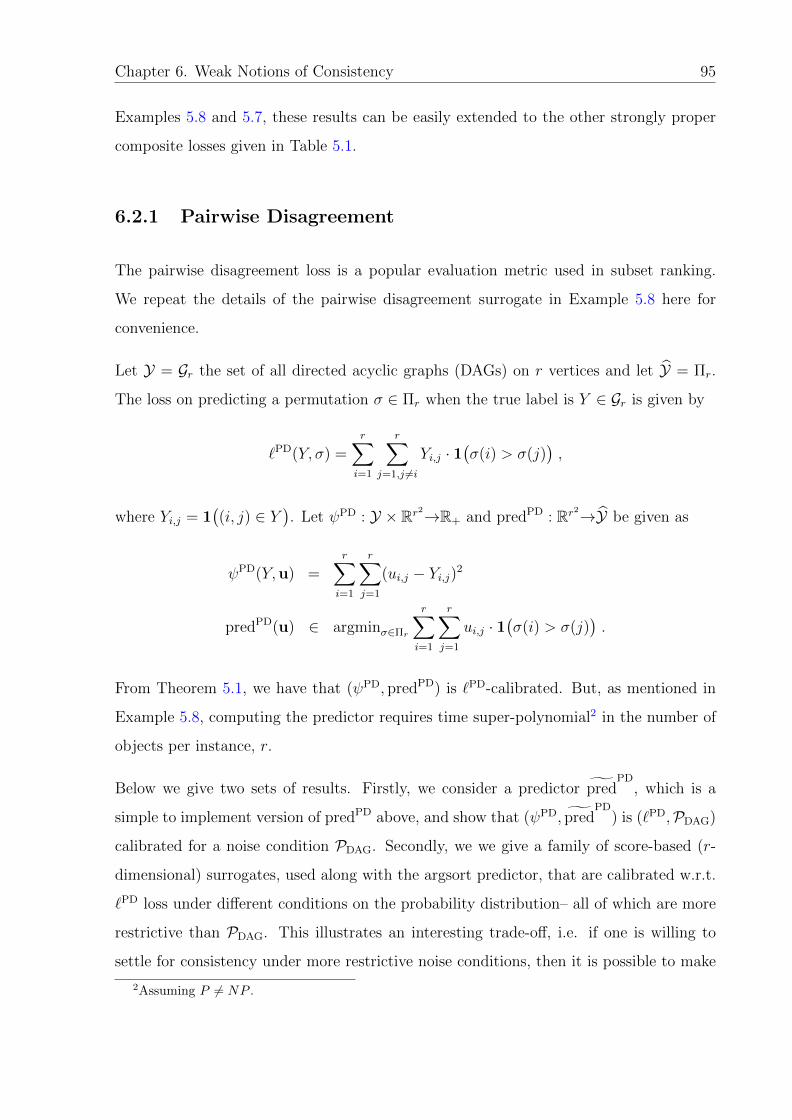
Chapter 6. Weak Notions of Consistency 95
Examples 5.8 and 5.7, these results can be easily extended to the other strongly proper
composite losses given in Table 5.1.
6.2.1 Pairwise Disagreement
The pairwise disagreement loss is a popular evaluation metric used in subset ranking.
We repeat the details of the pairwise disagreement surrogate in Example 5.8 here for
convenience.
Let Y = Gr the set of all directed acyclic graphs (DAGs) on r vertices and let Y = Πr.
The loss on predicting a permutation σ ∈ Πr when the true label is Y ∈ Gr is given by
`PD(Y, σ) =r∑i=1
r∑j=1,j 6=i
Yi,j · 1(σ(i) > σ(j)
),
where Yi,j = 1((i, j) ∈ Y
). Let ψPD : Y × Rr2→R+ and predPD : Rr2→Y be given as
ψPD(Y,u) =r∑i=1
r∑j=1
(ui,j − Yi,j)2
predPD(u) ∈ argminσ∈Πr
r∑i=1
r∑j=1
ui,j · 1(σ(i) > σ(j)
).
From Theorem 5.1, we have that (ψPD, predPD) is `PD-calibrated. But, as mentioned in
Example 5.8, computing the predictor requires time super-polynomial2 in the number of
objects per instance, r.
Below we give two sets of results. Firstly, we consider a predictor predPD
, which is a
simple to implement version of predPD above, and show that (ψPD, predPD
) is (`PD,PDAG)
calibrated for a noise condition PDAG. Secondly, we we give a family of score-based (r-
dimensional) surrogates, used along with the argsort predictor, that are calibrated w.r.t.
`PD loss under different conditions on the probability distribution– all of which are more
restrictive than PDAG. This illustrates an interesting trade-off, i.e. if one is willing to
settle for consistency under more restrictive noise conditions, then it is possible to make
2Assuming P 6= NP .

Chapter 6. Weak Notions of Consistency 96
both the surrogate optimization in the training phase, and predictor computation in the
prediction phase, computationally easier. These score-based surrogates and conditions
generalize the surrogate and noise condition of Duchi et al. [34].
6.2.1.1 DAG Based Surrogate
Observing the expression for predPD(u) carefully, one can see that the main reason for
the computational difficulty is that the graph given by u may not be acyclic, in which
case the problem becomes equivalent to feedback arc set. If the directed graph Y given
by u is indeed acyclic, then any permutation given by the topological sorted order of
Y , denoted by topsort(Y ), would satisfy the requirement of pred(u). Hence, if one can
ensure a noise condition such that it does not matter what the predictor does on inputs
u corresponding to cyclic graphs, then we immediately get an efficient predictor.
Consider the predictor predPD
: Rr2→Y that is described by Algorithm 1 below:
Algorithm 1 predPD
Input: u ∈ Rr2
Output: Permutation σ ∈ Πr
Construct a directed graph Y over [r] with edge (i, j) having weight (ui,j − uj,i)+.while Y has cycles
Delete the edge of Y with minimum weightend whilereturn topsort(Y )
Let ∆Y be the set of all distributions over the set of DAGs Y . For each p ∈ ∆Y , define
Ep = (i, j) ∈ [r]× [r] : EY∼p[Yi,j] > EY∼p[Yj,i], and define PDAG ⊂ ∆Y as follows:
PDAG =
p ∈ ∆Y :([r], Ep
)is a DAG
.
Then we have the following result:
Theorem 6.2. (ψPD, predPD
) is (`PD,PDAG)-calibrated.

Chapter 6. Weak Notions of Consistency 97
Proof. Let p ∈ PDAG. Define up ∈ Rr2 such that for all i, j ∈ [r]
upi,j = EY∼p[Yi,j] =∑y∈Y
pyyi,j .
It is easy to see that up is the unique minimizer of 〈p,ψPD(u) over u ∈ Rr2 .
Define the following sets:
Π∗(p) = argminσ∈Πr〈p, `PDσ 〉 = argminσ∈Sr
r∑i=1
r∑j=1
(upi,j) · 1(σ(i) > σ(j))
Π(p) =σ ∈ Πr : σ corresponds to any topological sorted order given by pred
PD.
We claim that Π(p) ⊆ Π∗(p). To see this, let σ ∈ Π(p). Since p ∈ PDAG, we have that
the graph with edge weights (upi,j − upj,i)+ formed by predPD
(up) is a DAG, and therefore
σ must agree with the edges in this graph, i.e.
upi,j > upj,i =⇒ σ(i) < σ(j) ,
upi,j < upj,i =⇒ σ(i) > σ(j) .
This clearly gives σ ∈ Π∗(p). Thus Π(p) ⊆ Π∗(p).
Now, let
A(p) =u ∈ Rr2 : pred
PD(u) /∈ argminσ〈p, `PD
σ 〉
=u ∈ Rr2 : pred
PD(u) /∈ Π∗(p)
.
To show that (ψPD, predPD
) is (`PD,PDAG)-calibrated, one simply needs to show:
infu∈A(p)
〈p,ψPD(u)〉 > infu∈Rr〈p,ψPD(u)〉 .
We do so by showing that any sequence um in Rr2 converging to up must eventually
lie outside A(p), i.e. that any such sequence must eventually have predPD
(um) ∈ Π∗(p);
the result will then follow from the fact that up is the unique minimizer of 〈p,ψPD(.)〉.
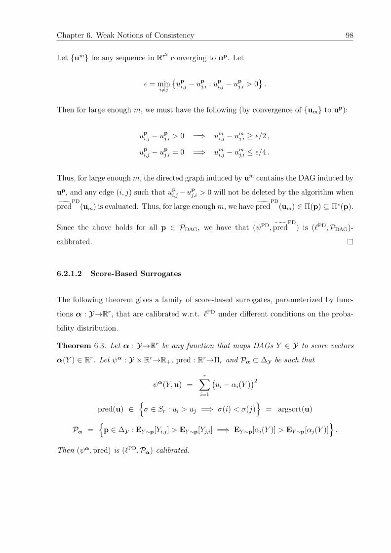
Chapter 6. Weak Notions of Consistency 98
Let um be any sequence in Rr2 converging to up. Let
ε = mini 6=j
upi,j − upj,i : upi,j − upj,i > 0
.
Then for large enough m, we must have the following (by convergence of um to up):
upi,j − upj,i > 0 =⇒ umi,j − umj,i ≥ ε/2 ,
upi,j − upj,i = 0 =⇒ umi,j − umj,i ≤ ε/4 .
Thus, for large enough m, the directed graph induced by um contains the DAG induced by
up, and any edge (i, j) such that upi,j −upj,i > 0 will not be deleted by the algorithm when
predPD
(um) is evaluated. Thus, for large enoughm, we have predPD
(um) ∈ Π(p) ⊆ Π∗(p).
Since the above holds for all p ∈ PDAG, we have that (ψPD, predPD
) is (`PD,PDAG)-
calibrated.
6.2.1.2 Score-Based Surrogates
The following theorem gives a family of score-based surrogates, parameterized by func-
tions α : Y→Rr, that are calibrated w.r.t. `PD under different conditions on the proba-
bility distribution.
Theorem 6.3. Let α : Y→Rr be any function that maps DAGs Y ∈ Y to score vectors
α(Y ) ∈ Rr. Let ψα : Y × Rr→R+, pred : Rr→Πr and Pα ⊂ ∆Y be such that
ψα(Y,u) =r∑i=1
(ui − αi(Y )
)2
pred(u) ∈σ ∈ Sr : ui > uj =⇒ σ(i) < σ(j)
= argsort(u)
Pα =
p ∈ ∆Y : EY∼p[Yi,j] > EY∼p[Yj,i] =⇒ EY∼p[αi(Y )] > EY∼p[αj(Y )].
Then (ψα, pred) is (`PD,Pα)-calibrated.

Chapter 6. Weak Notions of Consistency 99
Proof. Let p ∈ Pα. Define up ∈ Rr as
up = EY∼p[α(Y )] =∑y∈Y
pyα(y) .
It is easy to see that up is the unique minimizer of 〈p,ψα(u)〉 over u ∈ Rr.
Also define yp ∈ Rr2 such that for all i, j ∈ [r]
ypi,j = EY∼p[Yi,j] =∑y∈Y
pyyi,j .
Define the following sets:
Π∗(p) = argminσ∈Πr〈p, `PDσ 〉
= argminσ∈Πr
r∑i=1
r∑j=1
ypi,j · 1(σ(i) > σ(j))
Π(p) =σ ∈ Πr : upi > upj =⇒ σ(i) < σ(j)
.
We claim that Π(p) ⊆ Π∗(p). To see this, let σ ∈ Π(p). Since p ∈ Pα, we have
ypi,j > ypj,i =⇒ upi > upj =⇒ σ(i) < σ(j) ,
ypi,j < ypj,i =⇒ upi < upj =⇒ σ(i) > σ(j) .
This clearly gives σ ∈ Π∗(p). Thus Π(p) ⊆ Π∗(p).
By the definition of pred and Π(p), we also have that ∃ε > 0 such that for any u ∈ Rr,
‖u− up‖ < ε =⇒ pred(u) ∈ Π(p) .
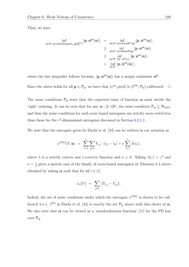
Chapter 6. Weak Notions of Consistency 100
Thus, we have
infu∈Rr:pred(u)/∈argminσ〈p,`PD
σ 〉〈p,ψα(u)〉 = inf
u∈Rr:pred(u)/∈Π∗(p)〈p,ψα(u)〉
≥ infu∈Rr:pred(u)/∈Π(p)
〈p,ψα(u)〉
≥ infu∈Rr:‖u−up‖≥ε
〈p,ψα(u)〉
> infu∈Rr〈p,ψα(u)〉 ,
where the last inequality follows because, 〈p,ψα(u)〉 has a unique minimizer up.
Since the above holds for all p ∈ Pα, we have that (ψα, pred) is (`PD,Pα)-calibrated.
The noise conditions Pα state that the expected value of function α must decide the
‘right’ ordering. It can be seen that for any α : Y→Rr, the noise condition Pα ( PDAG,
and thus the noise conditions for such score based surrogates are strictly more restrictive
than those for the r2-dimensional surrogates discussed in Section 6.2.1.1.
We note that the surrogate given by Duchi et al. [34] can be written in our notation as
ψDMJ(Y,u) =r∑i=1
∑j 6=i
Yi,j · (uj − ui) + νr∑i=1
λ(ui) ,
where λ is a strictly convex and 1-coercive function and ν > 0. Taking λ(z) = z2 and
ν = 12
gives a special case of the family of score-based surrogates in Theorem 6.3 above
obtained by taking α such that for all i ∈ [r]
αi(Y ) =∑j 6=i
(Yi,j − Yj,i
).
Indeed, the set of noise conditions under which the surrogate ψDMJ is shown to be cali-
brated w.r.t. `PD in Duchi et al. [34] is exactly the set Pα above with this choice of α.
We also note that α can be viewed as a ‘standardization function’ [11] for the PD loss
over Pα.

Chapter 6. Weak Notions of Consistency 101
6.2.2 Mean Average Precision
The mean average precision is another popular evaluation metric in ranking. We repeat
the details from Example 5.7 here for convenience.
Let Y = 0, 1r \ 0 and Y = Πr. The loss on predicting a permutation σ ∈ Πr when
the true label is y ∈ Y is given by
`MAP(y, σ) = 1− 1
‖y‖1
r∑i=1
i∑j=1
yi yjmax(σ(i), σ(j))
.
Let ψMAP : Y × R(r)(r+1)/2→R+ and predMAP : Rr→Y be such that
ψMAP(y,u) =r∑i=1
i∑j=1
(ui,j −
yiyj‖y‖1
)2
predMAP(u) ∈ argmaxσ∈Πr
r∑i=1
i∑j=1
ui,j ·1
max(σ(i), σ(j)).
From Theorem 5.1, we have that (ψMAP, predMAP) is `MAP-calibrated. But, as mentioned
in Example 5.7, computing the predictor is hard.
Below, we describe an alternate mapping in place of predMAP which can be computed
efficiently, and show that under certain conditions on the probability distribution, the
surrogate ψMAP together with this mapping is still calibrated for `MAP.
Specifically, define predMAP : Rr(r+1)/2→Y as follows:
predMAP
(u) ∈σ ∈ Πr : ui,i > uj,j =⇒ σ(i) < σ(j)
.
Clearly, predMAP
(u) can be implemented efficiently by simply sorting the ‘diagonal’ ele-
ments ui,i for i ∈ [r]. Also, let ∆Y denote the probability simplex over Y , and for each
p ∈ ∆Y , define up ∈ Rr(r+1)/2 as follows:
upi,j = EY∼p
[YiYj||Y ||1
]=∑y∈Y
py
(yiyj||y||1
)∀i, j ∈ [r] : i ≥ j .

Chapter 6. Weak Notions of Consistency 102
Now define PMAP ⊂ ∆Y as follows:
PMAP =
p ∈ ∆Y : upi,i ≥ upj,j =⇒ upi,i ≥ upj,j +∑
γ∈[r]\i,j(upjγ − upiγ)+
,
where we set upi,j = upj,i for i < j. Then we have the following result:
Theorem 6.4. (ψMAP, predMAP
) is (`MAP,PMAP)-calibrated.
Proof. Let p ∈ PMAP.
It is easy to see that up ∈ Rr(r+1)/2 is the unique minimizer of 〈p,ψMAP(u)〉 over u ∈Rr(r+1)/2.
We have from the definition of the MAP loss,
〈p, `MAPσ 〉 = 1−
r∑i=1
i∑j=1
upi,j1
max(σ(i), σ(j))
= 1−r∑i=1
1
i
i∑j=1
upσ−1(i)σ−1(j) . (6.1)
Now define the following sets:
Π∗(p) = argminσ∈Πr〈p, `MAPσ 〉
Π(p) =σ ∈ Πr : upi,i > upj,j =⇒ σ(i) < σ(j)
.
From Lemma 6.5 below, we have that Π(p) ⊆ Π∗(p).
By the definition of predMAP
and Π(p), we also have that ∃ε > 0 such that for any
u ∈ Rr(r+1)/2,
‖u− up‖ < ε =⇒ predMAP
(u) ∈ Π(p) .

Chapter 6. Weak Notions of Consistency 103
Thus, we have
infu∈Rr(r+1)/2:pred
MAP(u)/∈argminσ〈p,`σ〉
〈p,ψMAP(u)〉 = infu∈Rr(r+1)/2:pred
MAP(u)/∈Π∗(p)
〈p,ψMAP(u)〉
≥ infu∈Rr(r+1)/2:pred
MAP(u)/∈Π(p)
〈p,ψMAP(u)〉
≥ infu∈Rr(r+1)/2:‖u−up‖≥ε
〈p,ψMAP(u)〉
> infu∈Rr(r+1)/2
〈p,ψMAP(u)〉 ,
where the last inequality follows because 〈p,ψMAP(u)〉 has a unique minimizer up.
Since the above holds for all p ∈ PMAP, we have that (ψMAP, predMAP
) is (`MAP,PMAP)-
calibrated.
The proof of Theorem 6.4 makes use of the following technical lemma:
Lemma 6.5. Let p ∈ PMAP. Let the sets Π∗(p) and Π(p) be defined as in the proof of
Theorem 6.4 above. Then Π(p) ⊆ Π∗(p).
Proof of Lemma 6.5. We first observe that all permutations σ ∈ Π(p) have the same
value of 〈p, `MAPσ 〉. To see this, note that permutations in Π(p) differ only in positions
they assign to elements i, j ∈ [r] with upi,i = upj,j. But since p ∈ PMAP, we have that if
upi,i = upj,j, then upi,γ = upj,γ for all γ ∈ [r] \ i, j. Thus, from the form of 〈p, `MAPσ 〉, we
can see that if upi,i = upj,j, interchanging the positions of i and j in a permutation σ does
not change the value of 〈p, `MAPσ 〉. This establishes that all permutations σ ∈ Π(p) have
the same value of 〈p, `MAPσ 〉.
We will show below that ∃ a permutation σ∗ ∈ Π(p) ∩ Π∗(p). This will give that σ∗ ∈Π(p) and 〈p, `MAP
σ∗ 〉 = minσ〈p, `MAPσ 〉; by the above observation, we will then have that
〈p, `MAPσ′ 〉 = minσ〈p, `MAP
σ 〉 for all σ′ ∈ Π(p), i.e. that Π(p) ⊆ Π∗(p).
In order to show the existence of a permutation σ∗ ∈ Π(p) ∩ Π∗(p), we will start
with an arbitrary element σ0 ∈ Π∗(p), and will construct a sequence of permutations
σ1, σ2, . . . , σm = σ∗ by transposing one adjacent pair at a time, such that all elements in
the sequence remain in Π∗(p), and the final permutation σm is also in Π(p).

Chapter 6. Weak Notions of Consistency 104
Let σ0 ∈ Π∗(p). If σ0 ∈ Π(p), we are done, so let us assume σ0 /∈ Π(p). Thus there must
exist an adjacent pair of elements in σ that are not ordered according to the scores upi,i,
i.e. there must exist a, b, c ∈ [r] such that
σ0(a) = c, σ0(b) = c+ 1, and upa,a < upb,b .
Define σ1 to be such that σ1(a) = c+ 1, σ1(b) = c, and σ1(i) = σ0(i) for all other i ∈ [r].
We will show that σ1 ∈ Π∗(p). For convenience let us denote (σ0)−1 as π0 and (σ1)−1 as
π1. Note that
π0(c) = π1(c+ 1) = a
π0(c+ 1) = π1(c) = b
π0(i) = π1(i) ∀i ∈ [r] \ c, c+ 1 .
From the expression for 〈p, `MAPσ 〉 in Equation (6.1) in the proof of Theorem 6.4 above,
we have
〈p, `MAPσ0 〉 − 〈p, `MAP
σ1 〉
=1
c
(c∑j=1
(upπ1(c),π1(j) − upπ0(c),π0(j))
)+
1
c+ 1
(c+1∑j=1
(upπ1(c+1),π1(j) − upπ0(c+1),π0(j))
)
=1
c
(c∑j=1
(upb,π1(j) − upa,π0(j))
)+
1
c+ 1
(c+1∑j=1
(upa,π1(j) − upb,π0(j))
)
=
(1
c− 1
c+ 1
) c−1∑j=1
(upb,π1(j) − upa,π1(j)) +
1
c(upb,b − upa,a) +
1
c+ 1(upa,b + upa,a − upb,a − upb,b)
=
(1
c− 1
c+ 1
)( c−1∑j=1
(upb,π1(j) − upa,π1(j)) + upb,b − upa,a
)
=
(1
c− 1
c+ 1
)(upb,b −
(upa,a +
c−1∑j=1
(upa,π1(j) − upb,π1(j))
))
≥(
1
c− 1
c+ 1
)upb,b − (upa,a +∑
j∈[r],j /∈c,c+1(upa,π1(j) − u
pb,π1(j))+
)≥ 0 ,

Chapter 6. Weak Notions of Consistency 105
where the last inequality above follows since p ∈ PMAP. This gives σ1 ∈ Π∗(p). Moreover,
the number of pairs in σ1 that disagree with the ordering according to upi,i is one less than
that in σ0. Since there can be at most(r2
)such pairs in σ0 to start with, by repeating the
above process, we will eventually end up with a permutation σm ∈ Π(p) ∩ Π∗(p) (with
m ≤(r2
)). The claim follows.
The ideal predictor predMAP uses the entire u matrix, but the predictor predMAP
, uses only
the diagonal elements. The noise conditions PMAP can be viewed as basically enforcing
that the diagonal elements dominate and enforce a clear ordering themselves.
In fact, since the mapping predMAP
depends on only the diagonal elements of u, we can
equivalently define an r-dimensional surrogate that is calibrated w.r.t. `MAP over PMAP.
Specifically, we have the following immediate corollary:
Corollary 6.6. Let ψMAP : 0, 1r × Rr→R+ and pred : Rr→Πr be such that
ψMAP(y, u) =r∑i=1
(ui −
yi||y||1
)2
pred(u) ∈σ ∈ Πr : ui > uj =⇒ σ(i) < σ(j)
= argsort(u) .
Then (ψMAP, pred) is (`MAP,PMAP)-calibrated.
Looking at the form of ψMAP and pred, we can see that the function s : Y→Rr defined as
si(y) = yi/(||y||1) is a ‘standardization function’ for the MAP loss over PMAP, and there-
fore it follows that any ‘order-preserving surrogate’ with this standardization function is
also calibrated with the MAP loss over PMAP [11].
6.3 Approximate Consistency
Another approach to weakening the consistency requirement, distinct from assuming noise
conditions, is that of approximate consistency.
An algorithm returning a classifier hM : X→Y on being given a training sample of size
M , is said to be θ-approximately consistent if for any δ, ε > 0, we have that for large

Chapter 6. Weak Notions of Consistency 106
enough M , the folowing holds with with probability 1− δ:
er`D[hM ] ≤ θ · er`,∗D + ε .
For example, the 1-nearest neighbor algorithm is known to be 2-approximately consistent
for the zero-one loss used in classification [26].
We define the notion of approximate calibration of a surrogate, which implies approximate
consistency of the corresponding surrogate minimization algorithm.
Definition 6.2 (Approximate calibration). Let ` : Y × Y→R+ be a loss function. Let
ψ : Y × C→R+ and pred : C→Y. Let θ ≥ 1. We will say (ψ, pred) is θ-approximately
calibrated w.r.t. ` (or simply θ-approximately `-calibrated) if
∀p ∈ ∆n : infu∈C:〈p,`pred(u)〉>θmint〈p,`t〉
〈p,ψ(u)〉 > infu∈C〈p,ψ(u)〉 .
The following result shows that if (ψ, pred) is θ-approximately `-calibrated, then any
algorithm that is consistent w.r.t. ψ, and maps back its predictions in C to predictions in
Y via the mapping pred : C→Y , is also θ-approximately consistent w.r.t. `:
Theorem 6.7. Let ` : Y × Y→R+ be a loss function. Let ψ : Y × C→R+ and pred :
C→Y. Let θ > 1. If (ψ, pred) is θ-approximately `-calibrated, then for all distributions
D on X × Y and all sequences of (random) vector functions fm : X→C (depending on
(X1, Y1), . . . , (Xm, Ym)), as m→∞,
erψD[fm]P−→ erψ,∗D implies ∀ε > 0 : P
(er`D[pred fm] ≥ θ · er`,∗D + ε
)→ 0 .
Proof. The proof is similar to the proof of Theorem 3.2; we give an outline here for
completeness.
For each p ∈ ∆n, define Hpθ : R+→R+ as follows:
Hpθ (ε′) = inf
u∈Rd
〈p,ψ(u)〉 − inf
u′∈Rd〈p,ψ(u′)〉 : 〈p, `pred(u)〉 − θmin
t〈p, `t〉 ≥ ε′
.

Chapter 6. Weak Notions of Consistency 107
Since (ψ, pred) is θ-approximately `-calibrated, we have Hpθ (ε′) > 0 for all ε′ > 0 and
p ∈ ∆n. Now, define Hθ : R+→R+ as follows:
Hθ(ε′) = inf
p∈∆n,u∈Rd
〈p,ψ(u)〉 − inf
u′∈Rd〈p,ψ(u′)〉 : 〈p, `pred(u)〉 − θmin
t〈p, `t〉 ≥ ε′
.
The main step in the proof involves showing that we also have Hθ(ε′) > 0 for all ε′ > 0;
this can be established using arguments similar to those in the proof of Theorem 3.2. It
then follows that there exists a concave non-decreasing function ξ : R+→R+ with ξ(0) = 0
and continuous at 0, such that for all distributions D and functions f : X→Rd,
er`D[pred f ]− θ · er`,∗D ≤ ξ(erψD[f ]− erψ,∗D
).
The claim follows.
Below, we give two generic ways of constructing approximately calibrated surrogates and
predictors. The first way is to simply construct an exactly calibrated surrogate and
predictor for another loss matrix that closely approximates the loss of interest.
Theorem 6.8. Let ` : Y×Y→R+ and ˜ : Y×Y→R+ be loss functions such that ∃c1, c2 >
0, c2 ≥ c1, such that
c1˜(y, t) ≤ `(y, t) ≤ c2
˜(y, t) ∀y ∈ Y , t ∈ Y .
Let ψ : Y × Rd→R+ and pred : Rd→Y be such that (ψ, pred) is ˜-calibrated. Then
(ψ, pred) is(c2c1
)-approximately `-calibrated.
Proof. Let p ∈ ∆n. Let um be any sequence in Rd such that 〈p,ψ(um)〉 converges to
infu∈Rd〈p,ψ(u)〉. Then since (ψ, pred) is ˜-calibrated, we have that for large enough m,
〈p, ˜tm〉 = mint∈[k]〈p, ˜t〉 ,
where tm = pred(um). Now, for any t∗ satisfying 〈p, ˜t∗〉 = mint∈[k]〈p, ˜t〉, we have
∀t ∈ [k]:
〈p, `t∗〉 ≤ c2 〈p, ˜t∗〉 ≤ c2 〈p, ˜t〉 ≤ (c2
c1
)〈p, `t〉 .

Chapter 6. Weak Notions of Consistency 108
This gives that for large enough m, 〈p, `tm〉 ≤(c2c1
)mint∈[k]〈p, `t〉. Thus we have that
(ψ, pred) is(c2c1
)-approximately `-calibrated.
The second way of constructing approximately calibrated surrogates and predictors is
based on the generic loss matrix rank dimensional surrogate and predictor from Theorem
5.1. Recall that the predictor in that case was expressed as a discrete optimization
problem. Simply replacing it by a predictor that solves the discrete optimization problem
only to a factor θ of the best solution, gives an θ-approximately calibrated surrogate and
predictor.
Theorem 6.9. Let ` : Y × Y→R+. Let θ > 1. Suppose there exists d ∈ N, vectors
a1, a2, . . . , an ∈ [0, 1]d and b1,b2, . . . ,bk ∈ Rd and scalars c1, c2, . . . , cn, c1, c2, . . . , ck ∈ R
such that
`(y, t) = 〈ay,bt〉+ cy + ct .
Let V ⊆ R and let ρ : 1, 2 × V→R+ be a γ-strongly proper loss for some γ > 0 with a
link function λ : [0, 1]→V. Let the surrogate ψ : Y × Vd→R+ be given by
ψ(y,u) =d∑i=1
(ay,i)ρ(1, ui) + (1− ay,i)ρ(2, ui)
and let the predictor pred : Vd→Y be such that
〈λ−1(u),bpred(u)〉+ dpred(u) ≤ θ ·mint∈Y
(〈λ−1(u),bt〉+ ct
),
where [λ−1(u)]i = λ−1(ui). Then for all distributions D and functions f : X→Vd
er`D[pred f ] ≤ (θ + 1) maxt‖bt‖
√2
γregψD[f ] + θ min
h:X→Yer`D[h] .
In particular, (ψ, pred) is θ-approximately `-calibrated.
Proof. Let the matrix A ∈ [0, 1]d×n be given by A = [a1, a2, . . . , an]. Fix p ∈ ∆n,u ∈ Vd.Let t∗ ∈ Y be such that
⟨λ−1(u)−Ap,bt∗
⟩= max
t∈Y
(⟨λ−1(u)−Ap,bt
⟩).

Chapter 6. Weak Notions of Consistency 109
We then have that,
er`p(pred(u))
= 〈p, `pred(u)〉+ 〈p, c〉
=⟨Ap,bpred(u)
⟩+ cpred(u) + 〈p, c〉
=⟨Ap− λ−1(u),bpred(u)
⟩+⟨λ−1(u),bpred(u)
⟩+ cpred(u) + 〈p, c〉
≤⟨Ap− λ−1(u),bpred(u)
⟩+ θ ·min
t∈Y
(⟨λ−1(u),bt
⟩+ ct
)+ 〈p, c〉
=⟨Ap− λ−1(u),bpred(u)
⟩+ θ ·min
t∈Y
(⟨λ−1(u)−Ap,bt
⟩+ 〈Ap,bt〉+ ct
)+ 〈p, c〉
≤⟨Ap− λ−1(u),bpred(u)
⟩+ θ ·max
t∈Y
(⟨λ−1(u)−Ap,bt
⟩)+ θ ·min
t∈Y(〈Ap,bt〉+ ct) + 〈p, c〉
=⟨Ap− λ−1(u),bpred(u)
⟩+ θ ·
(⟨λ−1(u)−Ap,bt∗
⟩)+ θ ·min
t∈Y(〈Ap,bt〉+ ct) + 〈p, c〉
=⟨Ap− λ−1(u),bpred(u) − θbt∗
⟩+ θ ·min
t∈Y(〈Ap,bt〉+ ct) + 〈p, c〉
=⟨Ap− λ−1(u),bpred(u) − θbt∗
⟩+ θ ·min
t∈Y(〈Ap,bt〉+ ct + 〈p, c〉)
=⟨Ap− λ−1(u),bpred(u) − θbt∗
⟩+ θ ·min
t∈Yer`p(t)
≤ (θ + 1) · ‖Ap− λ−1(u)‖ ·maxt‖bt‖+ θ ·min
t∈Yer`p(t) . (6.2)
The last inequality above follows from Cauchy-Schwarz. Also, from Equation (5.2) from
the proof of Theorem 5.1, we have
regψp(u) ≥ γ
2‖Ap− λ−1(u)‖2 (6.3)
Putting Equations (6.2) and (6.3) together we have
er`p(pred(u)) ≤ (θ + 1) ·maxt‖bt‖ ·
√2
γregψp(u) + θ ·min
t∈Yer`p(t) .
The theorem follows from taking expectations and applying Jensen’s inequality to the
square root function.
We now give some example applications where approximate consistency can be achieved
using the above theorem by efficient training and prediction algorithms, but achieving
exact consistency is hard. Once again, we use the squared loss as the proper loss ρ for

Chapter 6. Weak Notions of Consistency 110
illustration, any other strongly proper convex surrogate like the logistic or exponential
loss in Table 5.1 can be used as well.
Example 6.2 (Pairwise disagreement on permutations). Consider the pairwise disagree-
ment loss discussed in Example 5.8. We constructed a calibrated surrogate and predictor
for the PD loss, however computing the predictor is equivalent to solving the feedback arc
set problem, which is not only NP-hard, but even hard to approximate.
Now, consider a variant of the PD loss where the label space Y = Y = Πr, the set of
permutations on [r]. In this case, one can express the PD loss on predicting a permutation
σ, when the true permutation is y as
`PD(y, σ) =r∑i=1
i−1∑j=1
1(y(i) < y(j)) · 1(σ(i) > σ(j)) + 1(y(i) > y(j)) · 1
(σ(i) < σ(j)) .
Let ψPD : Y × Rr(r−1)/2→R+ and predPD : Rr(r−1)/2→Y be such that
ψPD(y,u) =r∑i=1
i−1∑j=1
(uij − 1(y(i) < y(j)))2
predPD(u) ∈ argminσ∈Πr
r∑i=1
i−1∑j=1
ui,j · 1(σ(i) > σ(j)) + (1− ui,j) · 1(σ(i) < σ(j)) ,
From Theorem 5.1, we have that (ψPD, predPD) is `PD-calibrated. While solving the opti-
mization problem posed by predPD is still NP-Hard, due to the sum to 1 structure of the op-
posite edge weights ui,j and uj,i, efficient constant-factor approximation algorithms exist.
For example, the LP-based rounding procedure of Ailon et al. [3] achieves (in expectation)
a 2.5-factor approximation; by Theorem 6.9, this yields an efficient 2.5-approximately
calibrated surrogate and predictor.3
Example 6.3 (Graph-based multilabel classification - penalized selection). Consider the
problem of graph based multilabel prediction with penalized selection, considered in Exam-
ple 5.10. Let Y = Y = 0, 1r. Let G be a graph over [r] and dG be the shortest distance
3One can also in principle use the PTAS of Kenyon-Mathieu and Schudy [57] for this problem to geta better approximation factor, although this is more complicated to implement.
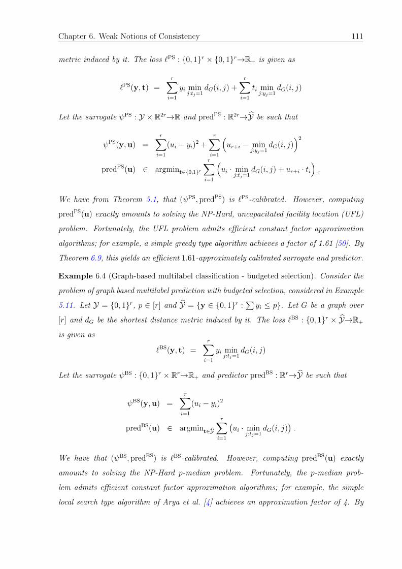
Chapter 6. Weak Notions of Consistency 111
metric induced by it. The loss `PS : 0, 1r × 0, 1r→R+ is given as
`PS(y, t) =r∑i=1
yi minj:tj=1
dG(i, j) +r∑i=1
ti minj:yj=1
dG(i, j)
Let the surrogate ψPS : Y × R2r→R and predPS : R2r→Y be such that
ψPS(y,u) =r∑i=1
(ui − yi)2 +r∑i=1
(ur+i − min
j:yj=1dG(i, j)
)2
predPS(u) ∈ argmint∈0,1rr∑i=1
(ui · min
j:tj=1dG(i, j) + ur+i · ti
).
We have from Theorem 5.1, that (ψPS, predPS) is `PS-calibrated. However, computing
predPS(u) exactly amounts to solving the NP-Hard, uncapacitated facility location (UFL)
problem. Fortunately, the UFL problem admits efficient constant factor approximation
algorithms; for example, a simple greedy type algorithm achieves a factor of 1.61 [50]. By
Theorem 6.9, this yields an efficient 1.61-approximately calibrated surrogate and predictor.
Example 6.4 (Graph-based multilabel classification - budgeted selection). Consider the
problem of graph based multilabel prediction with budgeted selection, considered in Example
5.11. Let Y = 0, 1r, p ∈ [r] and Y = y ∈ 0, 1r :∑yi ≤ p. Let G be a graph over
[r] and dG be the shortest distance metric induced by it. The loss `BS : 0, 1r × Y→R+
is given as
`BS(y, t) =r∑i=1
yi minj:tj=1
dG(i, j)
Let the surrogate ψBS : 0, 1r × Rr→R+ and predictor predBS : Rr→Y be such that
ψBS(y,u) =r∑i=1
(ui − yi)2
predBS(u) ∈ argmint∈Y
r∑i=1
(ui · min
j:tj=1dG(i, j)
).
We have that (ψBS, predBS) is `BS-calibrated. However, computing predBS(u) exactly
amounts to solving the NP-Hard p-median problem. Fortunately, the p-median prob-
lem admits efficient constant factor approximation algorithms; for example, the simple
local search type algorithm of Arya et al. [4] achieves an approximation factor of 4. By

Chapter 6. Weak Notions of Consistency 112
Theorem 6.9, this yields an efficient 4-approximately calibrated surrogate and predictor.

Part II
Application to
Hierarchical Classification

Chapter 7
Multiclass Classification with an
Abstain Option
In many applications like medical diagnosis, classification (binary or multiclass) is the
ultimate objective, but they have an additional requirement of having to make confident
decisions. In the event that they cannot make confident decisions, it is better to not
take any decision at all rather than make a wrong decision. For instance, in medical
diagnosis, if unable to predict the condition affecting the patient confidently using the
current symptoms and test reports, it is better to take further tests and postpone the
decision point, rather than making a prediction right away.
In other words, the prediction space Y contains the elements in Y to constitute a classifi-
cation problem, but it also contains a special element (which we denote by ⊥) indicating
the abstain option. Such problems are called multiclass (or binary) classification with an
abstain option and abbreviated for convenience as MCAO (or BCAO). This particular
type of supervised learning problem was also discussed in Example 2.4.
The problem of binary classification with an abstain option, has also been called ‘clas-
sification with a reject option’ and has been the object of study of many papers [6, 38–
41, 44, 47, 114]. In particular, Bartlett and Wegkamp [6], Grandvalet et al. [47], Yuan
and Wegkamp [114] assign a loss matrix of size 2×3 to this problem, and study consistent
surrogate minimization algorithms for this loss matrix.
114

Chapter 7. Abstain Loss 115
The loss function `α : Y×Y→R+, used by Bartlett and Wegkamp [6], Yuan and Wegkamp
[114], which we call the abstain(α) loss, for some Y with cardinality of 2, and Y = Y∪⊥and α ∈ [0, 1] is given as
`α(y, t) =
0 if y = t
α if t = ⊥
1 otherwise
(7.1)
Here α ∈ [0, 1] denotes the cost of abstaining. In the binary case, we have that for any
α > 12, it is never optimal to abstain and hence the only interesting range of values for α
is[0, 1
2
].
Yuan and Wegkamp [114] show that many standard smooth convex surrogates used in
binary classification, like the logistic surrogate, squared loss surrogate and exponential
loss surrogate are calibrated w.r.t. the above loss. Bartlett and Wegkamp [6] show that
the hinge loss is not calibrated with the above loss, but can be made calibrated with
a simple modification. The suggested modification is simply to use a double hinge loss
with three linear segments instead of the two segments in standard hinge loss, the ratio of
slopes of the two non-flat segments depends on the cost of abstaining α. Grandvalet et al.
[47] consider a slightly more general loss function than the above and derive a calibrated
double hinge surrogate loss for the same.
In many practical applications, one might require the abstain option with multiple classes,
i.e. to solve the MCAO problem, and it can be easily seen from Equation (7.1) that the
abstain(α) loss can just as easily be applied to the multiclass case with |Y| = n, as
in Example 2.10. While there have been some empirical and heuristic results for the
MCAO problem [93, 110, 117] there has been little theoretical analysis of the problem.
In particular, no known result exists on convex calibrated surrogates for such a loss with
n > 2, and none of the results for the binary case given above can be extended in a simple
way for n > 2.
The generic calibration result of Theorem 5.1, can be used to derive a (n−1)-dimensional
smooth convex calibrated surrogate for the abstain(α) loss for any α ∈ [0, n−1n
]. However

Chapter 7. Abstain Loss 116
such a smooth surrogate, essentially estimates the entire conditional probability vector
and does much more than what is necessary to solve this problem. On the other hand,
consistent piecewise linear surrogate minimizing algorithms do only what is needed and
can be expected to be more successful. For example, the squared loss, the logistic loss and
hinge loss surrogates are all calibrated w.r.t. standard 0-1 loss in binary classification, but
the support vector machine (which minimizes the piecewise linear hinge loss surrogate) is
arguably the most widely used method in binary classification. Piecewise linear surrogates
have other advantages like easier optimization and sparsity (in the dual) as well. This
motivates the question –
Are there natural piecewise linear convex calibrated surrogates for the n-class abstain(α)
loss generalizing those of Bartlett and Wegkamp [6] and Grandvalet et al. [47] ?
Another interesting object of study is the convex calibration dimension of the n-class
abstain(α) loss, which motivates the following question –
Is CCdim(`α) significantly less than n− 1 = CCdim(`0-1) ? If so what surrogate achieves
it?
In this chapter, we give positive answers to both questions. We construct three convex
calibrated piecewise-linear surrogates for the general n-class abstain(α) loss, for α ∈[0, 1
2
], all of which reduce to the double hinge surrogate of Bartlett and Wegkamp [6]
when n = 2, thus answering the first question. One of our constructed surrogates has a
surrogate dimension of dlog2(n)e, which answers the second question.
7.1 Chapter Organization
Firstly, we give some more detailed background on the abstain loss and discuss the effects
of α, the cost of abstaining in Section 7.2. We then show that the Crammer-Singer
(CS) surrogate [27] and one-vs-all hinge (OVA) surrogate [86] are calibrated w.r.t. the
abstain(12) loss in Sections 7.3 and 7.4, and also give excess risk bounds relating these
surrogates and the abstain(12) loss. We also design a new convex surrogate with surrogate
dimension log2(n) called the binary encoded predictions (BEP) surrogate and show that
it is calibrated with the abstain(12) loss, and give excess risk bounds relating this surrogate

Chapter 7. Abstain Loss 117
and the abstain(12) loss in Section 7.5. We give the details of a dual block co-ordinate
ascent algorithm for minimizing the BEP surrogate, in Section 7.6. We show how the
CS, OVA and BEP surrogates can be modified to be calibrated w.r.t. the abstain(α) loss
for any α ∈ [0, 12] in Section 7.7, and give experimental results for all three algorithms on
synthetic and real datasets in Section 7.8.
7.2 Background
In the rest of the chapter we shall fix Y = [n] for some n > 1 and Y = Y ∪ ⊥. For
the n-class abstain loss `α : Y × Y→R+ defined as in Equation (7.1), the Bayes optimal
classifier h∗α : X→Y is given as
h∗α(x) =
argmaxy∈[n] py(x) if maxy∈[n] py(x) ≥ 1− α
⊥ Otherwise
, (7.2)
The above can be seen as a natural extension of the ‘Chow’s rule’ [21] for the binary case.
It can also be seen that the interesting range of values for α is [0, n−1n
] as for all α > n−1n
the Bayes optimal classifier for the abstain(α) loss never abstains.
For small α, the classifier h∗α acts as a high-confidence classifier and would be useful in
applications like medical diagnosis. For example, if one wishes to learn a classifier for
diagnosing an illness with 80% confidence, and recommend further medical tests if it is
not possible, the ideal classifier would be h∗0.2, which is the minimizer of the abstain(0.2)
loss. If α = 12, the Bayes classifier h∗α has a very appealing structure – a class y ∈ [n] is
predicted only if the class y has a simple majority. The abstain(α) loss is also useful in
applications where a ‘greater than 1−α conditional probability detector’ can be used as a
black box. As we shall see in Chapter 8, a greater than 12
conditional probability detector
plays a crucial role in the Bayes optimal classifier for a hierarchical classification problem,
and hence any surrogate calibrated w.r.t. abstain(12) loss can be used as a component to
derive calibrated surrogates for hierarchical classification.

Chapter 7. Abstain Loss 118
(1, 0, 0) (0, 0, 1)
(0, 1, 0)
Q1
Q2
Q⊥
Q3
(23,13, 0)
(23, 0,13)
(0, 13,23)
(13, 0,23)
(13,23, 0) (0, 23,
13)
(a) α = 13
(1, 0, 0) (0, 0, 1)
(0, 1, 0)
Q1
Q2
Q⊥Q3
(12,12, 0)
(12, 0,12)
(0, 12,12)
(b) α = 12
(1, 0, 0) (0, 0, 1)
(0, 1, 0)
Q1
Q2
Q⊥
Q3
(12,12, 0)
(12, 0,12)
(0, 12,12)
(25 ,25 ,
15)
(15 ,25 ,
25)
(25 ,15 ,
25)
(c) α = 35
Figure 7.1: Trigger probability sets for the abstain(α) loss.
The generic calibrated surrogate of Theorem 5.1 can be made to be calibrated with any
α ∈ [0, n−1n
]. However, as we shall see, the CS, OVA and the BEP surrogates are only
calibrated w.r.t. abstain(12) loss. For any fixed α ∈ [0, 1
2], all these three surrogates can
be modified to be calibrated w.r.t. the abstain(α) loss , but they cannot be modified
to be made calibrated with the abstain(α) loss for α ∈ (12, n−1
n]. While this is slightly
restrictive, we argue that MCAO problems are typically applicable in situations where
high confidence (>50%) in the decisions are required, and these exactly correspond to
α ∈ [0, 12].
We also suspect that, abstain(α) problems with α > 12
are fundamentally more difficult
than those with α ≤ 12, for the reason that evaluating the Bayes classifier h∗α(x) can be
done for α ≤ 12
without finding the maximum conditional probability – just check if any
class has conditional probability greater than (1 − α) as there can only be one. This is
also evidenced by the more complicated trigger probability sets for the abstain(α) loss
with α > 12
as shown in Figure 7.1.
7.3 Excess Risk Bounds for the CS Surrogate
In this section we give an excess risk bound relating the abstain(12) loss `
12 , with the
Crammer-Singer surrogate ψCS [27], thereby showing that the CS surrogate is calibrated
w.r.t. the abstain(12) loss.

Chapter 7. Abstain Loss 119
Define the surrogate ψCS : Y × Rn→R+ and predictor predCSτ : Rn→Y as
ψCS(y,u) = (maxj 6=y
uj − uy + 1)+
predCSτ (u) =
argmaxi∈[n] ui if u(1) − u(2) > τ
⊥ otherwise
,
where u(i) is the ith element of the components of u when sorted in descending order and
τ ∈ (0, 1) is a threshold parameter. Informally, this predictor chooses the class i with the
highest score ui if it is the clear maximum, and abstains otherwise.
We now give the excess risk bound relating ψCS and `12 , which implies that (ψCS, predCS)
is `12 -calibrated.
Theorem 7.1. Let τ ∈ (0, 1) and α = 12. Then for all f : X→Rn
reg`α
D [predCSτ f ] ≤
(regψ
CS
D [f ])
2 min(τ, 1− τ).
The following lemma gives some straightforward to prove, (in)equalities satisfied by the
Crammer-Singer surrogate and will play an important role in the proof of the Theorem
above.
Lemma 7.2.
∀y ∈ [n], ∀p ∈ ∆n
〈p,ψCS(eny )〉 = 2(1− py), (7.3)
〈p,ψCS(0)〉 = 1, (7.4)
∀u ∈ Rn, ∀y ∈ argmaxi ui ,∀y′ /∈ argmaxi ui
ψCS(y,u) ≥ u(2) − u(1) + 1, (7.5)
ψCS(y′,u) ≥ u(1) − u(2) + 1, (7.6)
where eny is the vector in Rn with 1 in the yth position and 0 everywhere else.
Proof. (Proof of Theorem 7.1)

Chapter 7. Abstain Loss 120
We will show that ∀p ∈ ∆n and all u ∈ Rn
regψCS
p (u) ≥ 2 min(τ, 1− τ) · reg`α
p (predCSτ (u)) . (7.7)
The Theorem simply follows from linearity of expectation.
Define the sets U τ1 , . . . ,U τn ,U τ⊥ such that for any t ∈ Y
U τt = u ∈ Rn : predCSτ (u) = t .
These sets evaluate to
U τt = u ∈ Rn : uy > uj + τ for all j 6= y; t ∈ [n]
U τ⊥ = u ∈ Rn : u(1) ≤ u(2) + τ.
Case 1: py ≥ 12
for some y ∈ [n].
We have that y ∈ argmint〈p, `αt 〉.
Case 1a: u ∈ U τy
The RHS of Equation (7.7) is zero, and hence becomes trivial.
Case 1b: u ∈ U τ⊥
We have that u(1) − u(2) ≤ τ .
Let q =∑
i∈argmaxj ujpi. We then have
regψCS
p (u) ≥ 〈p,ψCS(u)〉 − 〈p,ψCS(eny )〉(7.3)=
∑i:ui=u(1)
piψCS(i,u) +
∑i:ui<u(1)
pyψCS(y,u)− 2(1− py)
(7.5),(7.6)
≥ (2q − 1)(u(2) − u(1))− 1 + 2py
≥ (2py − 1)(u(2) − u(1))− 1 + 2py
≥ (2py − 1)(1− τ) . (7.8)

Chapter 7. Abstain Loss 121
The next to last inequality is due to the observation that, if q > py then u(1) = u(2).
We also have that,
reg`α
p (predCSτ (u)) = 〈p, `α⊥〉 − 〈p, `αy 〉 = py −
1
2(7.9)
From Equations (7.8) and (7.9) we have
regψCS
p (u) ≥ 2(1− τ)(reg`
α
p (predCSτ (u))
)(7.10)
Case 1c: u ∈ Rn \ (U τy ∪ U τ⊥)
We have predCSτ (u) = y′ 6= y. Also py′ ≤ 1− py ≤ 1
2and u(1) = uy′ > u(2) + τ .
regψCS
p (u) ≥ 〈p,ψCS(u)〉 − 〈p,ψCS(eny )〉(7.3)=
(n∑
i=1;i 6=y′piψ
CS(i,u) + py′ψCS(y′,u)
)− 2(1− py)
(7.5),(7.6)
≥ (1− 2py′)(uy′ − u(2))− 1 + py
≥ 2τ(py − py′) (From Case 1c) (7.11)
We also have that
reg`α
p (predCSτ (u)) = 〈p, `αy′〉 − 〈p, `αy 〉 = py − py′ . (7.12)
From Equations (7.11) and (7.12) we have
regψCS
p (u) ≥ 2τ ·(reg`
α
p (predCSτ (u))
). (7.13)
Case 2: py′ <12
for all y′ ∈ [n]
We have that ⊥ ∈ argmint〈p, `αt 〉.
Case 2a: u ∈ U τ⊥ (or predCSτ (u) = ⊥)
The RHS of Equation (7.7) is zero, and hence becomes trivial.

Chapter 7. Abstain Loss 122
Case 2b: u ∈ Rn \ U τ⊥ (or predCSτ (u) 6= ⊥)
Let predCSτ (u) = argmaxi ui = y. We have that u(1) = uy > u(2) + τ and py <
12.
regψCS
p (u) ≥ 〈p,ψCS(u)〉 − 〈p,ψCS(0)〉(7.4)=
(n∑
i=1;i 6=ypiψ
CS(i,u) + pyψCS(y,u)
)− 1
(7.5),(7.6)
≥ (1− 2py)(u(1) − u(2))
≥ (1− 2py)(τ) (From Case 2b) . (7.14)
We also have that
reg`α
p (predCSτ (u)) = 〈p, `αy 〉 − 〈p, `α⊥〉 =
1
2− py (7.15)
From Equations (7.14) and (7.15) we have
regψCS
p (u) ≥ 2τ ·(reg`
α
p (predCSτ (u))
)(7.16)
Equation (7.7), and hence the Theorem, follows from Equations (7.10), (7.13) and (7.16).
7.4 Excess Risk Bounds for the OVA Surrogate
In this section we give an excess risk bound relating the abstain(12) loss `
12 , with the
one-vs-all hinge [86] surrogate, thereby showing that it is calibrated w.r.t. the abstain(12)
loss.
The surrogate ψOVA : Y × Rn→R+ and predictor predOVAτ : Rn→Y are defined as
ψOVA(y,u) =n∑i=1
1(y = i)(1− ui)+ + 1(y 6= i)(1 + ui)+
predOVAτ (u) =
argmaxi∈[n] ui if maxj uj > τ
⊥ otherwise
,

Chapter 7. Abstain Loss 123
where τ ∈ (−1, 1) is a threshold parameter, and ties are broken arbitrarily, say, in favor of
the label y with the smaller index. Informally, this predictor chooses the class i with the
highest score ui if at least one of the classes have a large score, and abstains otherwise.
We now give the excess risk bound relating ψOVA and `12 .
Theorem 7.3. Let τ ∈ (−1, 1) and α = 12. Then for all f : X→Rn
reg`α
D [predOVAτ f ] ≤
(regψ
OVA
D [f ])
2(1− |τ |) .
The following lemma gives some straightforward to prove, (in)equalities satisfied by the
OVA hinge surrogate and will play a crucial role in the proof of the Theorem above.
Lemma 7.4.
∀y ∈ [n],∀p ∈ ∆n ,∀u ∈ Rn
〈p,ψOVA(2 · eny − 1n)〉 = 4(1− py) (7.17)
〈p,ψOVA(−1n)〉 = 2 (7.18)
ψOVA(y,u) ≥∑j∈[n]
uj − 2uy + n , (7.19)
where eny is the vector in Rn with 1 in the yth position and 0 everywhere else.
Proof. (Proof of Theorem 7.3)
We will show that ∀p ∈ ∆n and all u ∈ [−1,∞)n
regψOVA
p (u) ≥ 2(1− |τ |) ·(reg`
α
p (predOVAτ (u))
). (7.20)
The Theorem simply follows from the observation that for all u ∈ Rn clipping the com-
ponents of u below −1 to −1 does not increase ψOVA(y,u) for any y and also does not
change predOVAτ (u).
Define the sets U τ1 , . . . ,U τn ,U τ⊥ such that for any t ∈ Y
U τt = u ∈ Rn : predOVAτ (u) = t .

Chapter 7. Abstain Loss 124
This evaluates to,
U τt = u ∈ Rn : uy > τ, y = argmaxi∈[n] ui, t ∈ [n]
U τ⊥ = u ∈ Rn : uj ≤ τ for all j ∈ [n].
Case 1: py ≥ 12
for some y ∈ [n].
We have that y ∈ argmint〈p, `αt 〉.
Case 1a: u ∈ [−1,∞)n ∩ U τy
The RHS of Equation (7.20) is zero, and hence becomes trivial.
Case 1b: u ∈ [−1,∞)n ∩ U τ⊥
We have that maxj uj ≤ τ .
regψOVA
p (u) ≥ 〈p,ψOVA(u)〉 − 〈p,ψOVA(2eny − 1n)〉(7.17)= 〈p,ψOVA(u)〉 − 4(1− py)
(7.19)
≥n∑i=1
(1− 2pi)ui + n− 4(1− py)
≥∑
i∈[n]\y(1− 2pi)ui + (2py − 1)(−τ) + n− 4(1− py)
≥∑i∈[n]
(2pi − 1) + (2py − 1)(−τ − 1) + n− 4(1− py)
= (2py − 1)(1− τ) . (7.21)
We also have
reg`α
p (predOVAτ (u)) = 〈p, `α⊥〉 − 〈p, `αy 〉 = py −
1
2. (7.22)
From Equations (7.21) and (7.22) we have for all u ∈ [−1,∞)n ∩ U τ⊥
regψOVA
p (u) ≥ 2(1− τ)(reg`
α
p (predOVAτ (u))
). (7.23)
Case 1c: u ∈ [−1,∞)n \ (U τy ∪ U τ⊥)

Chapter 7. Abstain Loss 125
We have predOVAτ (u) = y′ 6= y. Also py′ ≤ 1
2; uy′ > τ and uy′ ≥ uy.
regψOVA
p (u) ≥ 〈p,ψOVA(u)〉 − 〈p,ψOVA(2 · eny − 1n)〉(7.17)= 〈p,ψOVA(u)〉 − 4(1− py)
(7.19)
≥(
n∑i=1
(1− 2pi)ui + n
)− 4(1− py)
≥
∑i∈[n]\y′
(1− 2pi)ui + (1− 2py′)(τ) + n
− 4(1− py)
≥
∑i∈[n]
(2pi − 1) + (1− 2py′)(τ + 1) + n
− 4(1− py)
≥ 2(1 + τ)(py − py′) . (7.24)
We also have that
reg`α
p (predOVAτ (u)) = 〈p, `αy′〉 − 〈p, `αy 〉 = py − py′ . (7.25)
From Equations (7.24) and (7.25) we have for all u ∈ [−1,∞)n \ (U τy ∪ U τ⊥)
regψOVA
p (u) ≥ 2(1 + τ)(reg`
α
p (predOVAτ (u))
). (7.26)
Case 2: py′ <12
for all y′ ∈ [n]
We have that ⊥ ∈ argmint〈p, `t〉
Case 2a: u ∈ U τ⊥
The RHS of Equation (7.7) is zero, and hence becomes trivial.
Case 2b: u ∈ [−1,∞)n \ U τ⊥
Let predOVAτ (u) = argmaxi ui = y. We have that uy ≥ τ and py <
12.
regψOVA
p (u) ≥ 〈p,ψOVA(u)〉 − 〈p,ψOVA(−1n)〉(7.18)=
(〈p,ψOVA(u)〉
)− 2
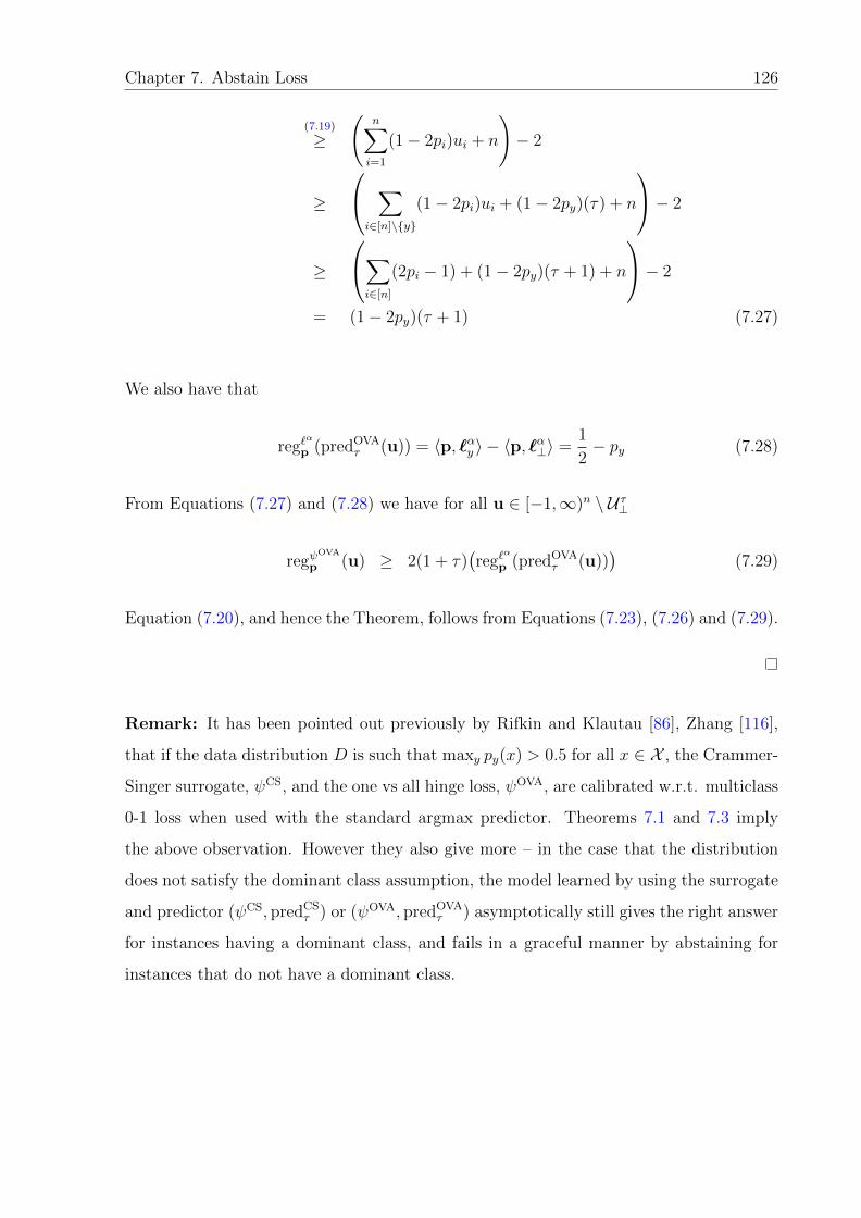
Chapter 7. Abstain Loss 126
(7.19)
≥(
n∑i=1
(1− 2pi)ui + n
)− 2
≥
∑i∈[n]\y
(1− 2pi)ui + (1− 2py)(τ) + n
− 2
≥
∑i∈[n]
(2pi − 1) + (1− 2py)(τ + 1) + n
− 2
= (1− 2py)(τ + 1) (7.27)
We also have that
reg`α
p (predOVAτ (u)) = 〈p, `αy 〉 − 〈p, `α⊥〉 =
1
2− py (7.28)
From Equations (7.27) and (7.28) we have for all u ∈ [−1,∞)n \ U τ⊥
regψOVA
p (u) ≥ 2(1 + τ)(reg`
α
p (predOVAτ (u))
)(7.29)
Equation (7.20), and hence the Theorem, follows from Equations (7.23), (7.26) and (7.29).
Remark: It has been pointed out previously by Rifkin and Klautau [86], Zhang [116],
that if the data distribution D is such that maxy py(x) > 0.5 for all x ∈ X , the Crammer-
Singer surrogate, ψCS, and the one vs all hinge loss, ψOVA, are calibrated w.r.t. multiclass
0-1 loss when used with the standard argmax predictor. Theorems 7.1 and 7.3 imply
the above observation. However they also give more – in the case that the distribution
does not satisfy the dominant class assumption, the model learned by using the surrogate
and predictor (ψCS, predCSτ ) or (ψOVA, predOVA
τ ) asymptotically still gives the right answer
for instances having a dominant class, and fails in a graceful manner by abstaining for
instances that do not have a dominant class.

Chapter 7. Abstain Loss 127
7.5 The BEP Surrogate
The Crammer-Singer surrogate and the one vs all hinge surrogate have a surrogate dimen-
sion of n. Thus any algorithm that minimizes these surrogates must learn n real valued
functions over the instance space. In this section, we construct a dlog2(n)e dimensional
convex surrogate, which we call as the binary encoded predictions (BEP) surrogate and
give an excess risk bound relating this surrogate and the abstain(12) loss. In particular
these results show that the BEP surrogate is calibrated w.r.t. the abstain loss; this in
turn implies that CCdim(`12 ) ≤ dlog2(n)e.
For the purpose of simplicity let us assume n = 2d for some d ∈ N.1 Let b : [n]→+1,−1d
be any one-one and onto mapping, with an inverse mapping b−1 : +1,−1d→[n]. For
any j ∈ [d], let bj : [n]→+1,−1 be the jth component of b. Define the BEP surrogate
ψBEP : Y × Rd→R+ and its corresponding predictor predBEPτ : Rd→Y as
ψBEP(y,u) = (maxj∈[d]
bj(y) · uj + 1)+
predBEPτ (u) =
⊥ if mini∈[d] |ui| ≤ τ
b−1(sign(−u)) Otherwise
where sign(u) is the sign of u, with sign(0) = 1 and τ ∈ (0, 1) is a threshold parameter.
Below we give an example construction of the BEP surrogate and predictor for a fixed n,
and also illustrate the predictor.
Example 7.1 (BEP surrogate for n = 4). Consider the surrogate and predictor look for
the case of n = 4 and τ = 12. We have d = 2. Let us fix the mapping b such that b(y) is
the standard d-bit binary representation of (y − 1), with −1 in the place of 0. Then we
have,
ψBEP(1,u) = (max(−u1,−u2) + 1)+
ψBEP(2,u) = (max(−u1, u2) + 1)+
1If n is not a power of 2, just add enough dummy classes that never occur.
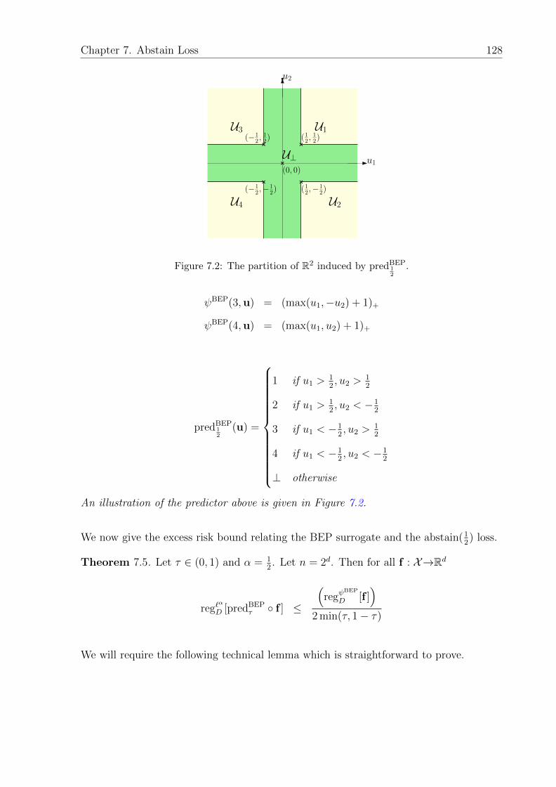
Chapter 7. Abstain Loss 128
(0, 0)
(−12 ,
12)
(−12 ,−1
2)
(12 ,12)
(12 ,−12)
U⊥
U3 U1
U4 U2
u2
u1
Figure 7.2: The partition of R2 induced by predBEP12
.
ψBEP(3,u) = (max(u1,−u2) + 1)+
ψBEP(4,u) = (max(u1, u2) + 1)+
predBEP12
(u) =
1 if u1 >12, u2 >
12
2 if u1 >12, u2 < −1
2
3 if u1 < −12, u2 >
12
4 if u1 < −12, u2 < −1
2
⊥ otherwise
An illustration of the predictor above is given in Figure 7.2.
We now give the excess risk bound relating the BEP surrogate and the abstain(12) loss.
Theorem 7.5. Let τ ∈ (0, 1) and α = 12. Let n = 2d. Then for all f : X→Rd
reg`α
D [predBEPτ f ] ≤
(regψ
BEP
D [f ])
2 min(τ, 1− τ)
We will require the following technical lemma which is straightforward to prove.
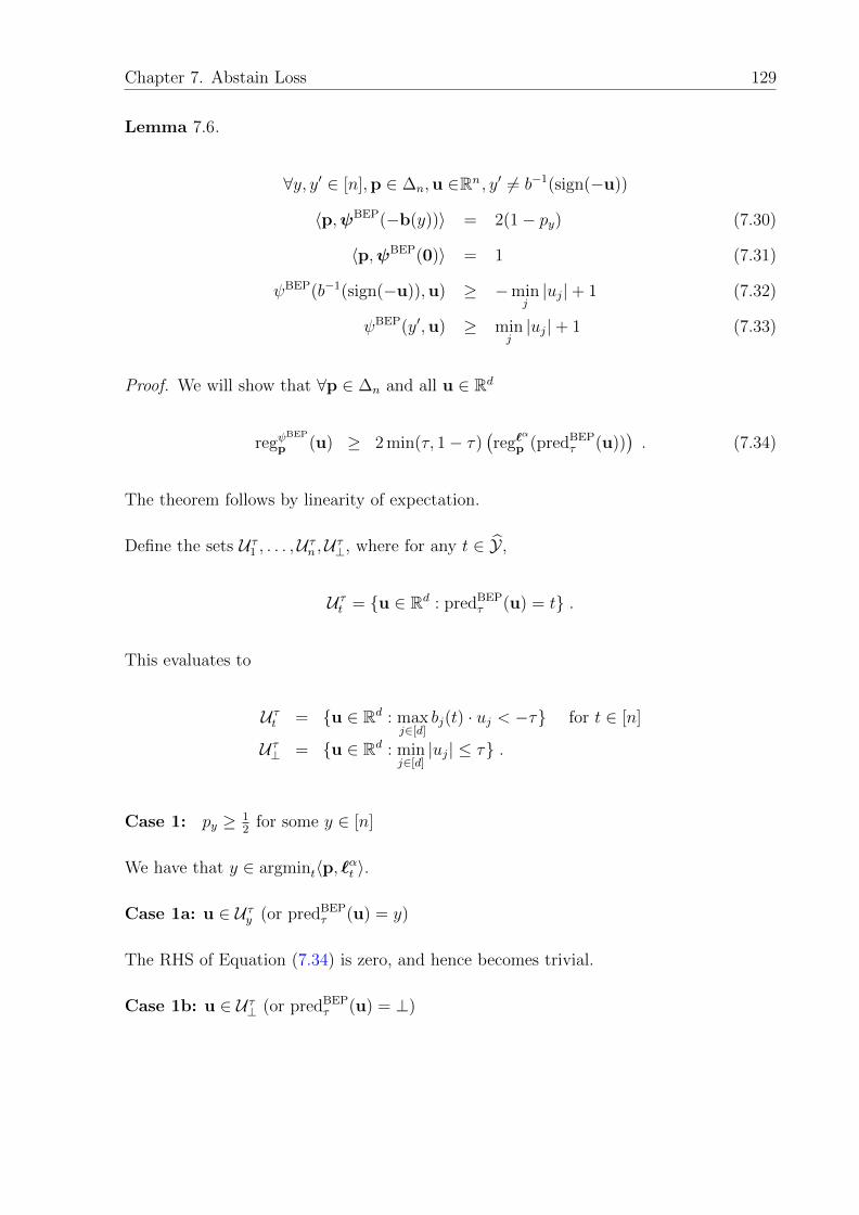
Chapter 7. Abstain Loss 129
Lemma 7.6.
∀y, y′ ∈ [n],p ∈ ∆n,u ∈Rn , y′ 6= b−1(sign(−u))
〈p,ψBEP(−b(y))〉 = 2(1− py) (7.30)
〈p,ψBEP(0)〉 = 1 (7.31)
ψBEP(b−1(sign(−u)),u) ≥ −minj|uj|+ 1 (7.32)
ψBEP(y′,u) ≥ minj|uj|+ 1 (7.33)
Proof. We will show that ∀p ∈ ∆n and all u ∈ Rd
regψBEP
p (u) ≥ 2 min(τ, 1− τ)(reg`
α
p (predBEPτ (u))
). (7.34)
The theorem follows by linearity of expectation.
Define the sets U τ1 , . . . ,U τn ,U τ⊥, where for any t ∈ Y ,
U τt = u ∈ Rd : predBEPτ (u) = t .
This evaluates to
U τt = u ∈ Rd : maxj∈[d]
bj(t) · uj < −τ for t ∈ [n]
U τ⊥ = u ∈ Rd : minj∈[d]|uj| ≤ τ .
Case 1: py ≥ 12
for some y ∈ [n]
We have that y ∈ argmint〈p, `αt 〉.
Case 1a: u ∈ U τy (or predBEPτ (u) = y)
The RHS of Equation (7.34) is zero, and hence becomes trivial.
Case 1b: u ∈ U τ⊥ (or predBEPτ (u) = ⊥)

Chapter 7. Abstain Loss 130
Let y′ = b−1(sign(−u)). We have minj |uj| ≤ τ .
regψBEP
p (u) ≥ 〈p,ψBEP(u)〉 − 〈p,ψBEP(−b(y))〉
(7.30)=
py′ψBEP(y′,u) +∑
i∈[n]\y′piψ
BEP(i,u)
− 2(1− py)
(7.32),(7.33)
≥(py′(−min
j∈[d]|uj|) + (1− py′)(min
j∈[d]|uj|) + 1
)− 2(1− py)
= (2py′ − 1)(−minj∈[d]|uj|) + 1− 2(1− py)
≥ (2py − 1)(−minj∈[d]|uj|) + 1− 2(1− py)
≥ (2py − 1)(−τ) + 1− 2(1− py)
= (2py − 1)(1− τ) . (7.35)
We also have that
reg`α
p (predBEPτ (u)) = 〈p, `α⊥〉 − 〈p, `αy 〉 = py −
1
2. (7.36)
From Equations (7.35) and (7.36) we have that
regψBEP
p (u) ≥ 2(1− τ)(reg`α
p (predBEPτ (u))) . (7.37)
Case 1c: u ∈ Rd \ (U τy ∪ U τ⊥)
Let b−1(sign(−u)) = pred(u) = y′ for some y′ 6= y. We have py′ ≤ 1 − py ≤ 12, and
minj |uj| > τ and
regψBEP
p (u) ≥ 〈p,ψBEP(u)〉 − 〈p,ψBEP(−b(y))
(7.30)
≥ py′ψBEP(y′,u) +
n∑i=1;i 6=y′
piψBEP(i,u)− 2(1− py)
(7.32),(7.33)
≥ py′(−minj|uj|) + (1− py′)(min
j|uj|) + 1− 2(1− py)
≥ τ(1− 2py′) + 1− 2(1− py) (From case 1c)

Chapter 7. Abstain Loss 131
≥ τ(1− 2py′) + 2py − 1
≥ τ(1− 2py′) + τ(2py − 1)
= 2τ(py − py′) . (7.38)
We also have that
reg`α
p (predBEPτ (u)) = 〈p, `αy′〉 − 〈p, `αy 〉 = py − py′ . (7.39)
From Equations (7.38) and (7.39) we have that
regψBEP
p (u) ≥ 2(τ)(reg`α
p (predBEPτ (u))) . (7.40)
Case 2: py <12
for all y ∈ [n]
We have that ⊥ ∈ argmint〈p, `αt 〉
Case 2a: u ∈ U τ⊥
The RHS of Equation (7.34) is zero, and hence becomes trivial.
Case 2b: u ∈ Rd \ U τ⊥
Let b−1(sign(−u)) = y′ = predBEPτ (u) for some y′ ∈ [n]. We have py′ <
12
and minj |uj| >τ .
regψBEP
p (u) ≥ 〈p,ψBEP(u)〉 − 〈p,ψBEP(0)〉(7.31)= py′ψ
BEP(y′,u) +n∑
i=1;i 6=y′piψ
BEP(i,u)− 1
(7.32),(7.33)
≥ −py′ minj|uj|+ (1− py′) min
j|uj|
≥ (1− 2py′)τ (7.41)
We also have that
reg`α
p (predBEPτ (u)) = 〈p, `αy′〉 − 〈p, `α⊥〉 =
1
2− py′ . (7.42)

Chapter 7. Abstain Loss 132
From Equations (7.41) and (7.42) we have that
regψBEP
p (u) ≥ 2τ(reg`α
p (predBEPτ (u))) . (7.43)
Equation (7.34), and hence the Theorem, follows from equations (7.37), (7.40) and (7.43).
7.6 BEP Surrogate Optimization Algorithm
In this section, we frame the problem of finding the linear (vector valued) function that
minimizes the BEP surrogate loss over a training set (xi, yi)Mi=1, with xi ∈ Ra and
yi ∈ [n], as a convex optimization problem. Once again, for simplicity we assume that
the size of the label space n = 2d for some d ∈ Z+. The primal and dual of the resulting
optimization problem with a norm squared regularizer is given below:
Primal problem:
minw1,...,wd,ξ1,...,ξM
M∑i=1
ξi +λ
2
d∑j=1
||wj||2
such that ∀i ∈ [M ], j ∈ [d]
ξi ≥ bj(yi)w>j xi + 1
ξi ≥ 0
Dual problem:
maxα−
M∑i=1
αi,0 −1
2λ
M∑i=1
M∑i′=1
〈xi,xi′〉µi,i′(α)
such that ∀i ∈ [M ], j ∈ [d] ∪ 0
αi,j ≥ 0;d∑
j′=0
αi,j′ = 1 .
where µi,i′(α) =∑d
j=1 bj(yi)bj(yi′)αijαi′,j.
We optimize the dual as it can be easily extended to work with kernels. The structure of
the constraints in the dual lends itself easily to a block co-ordinate ascent algorithm, where
we optimize over αi,j : j ∈ 0, . . . , d and fix every other variable in each iteration. Such
methods have been recently proven to have exponential convergence rate for SVM-type
problems [107], and we expect results of those type to apply to our problem as well.
The problem to be solved at every iteration reduces to an `2 projection of a vector gi ∈ Rd
on to the set Si = g ∈ Rd : 〈g,b(yi)〉 ≤ 1. The projection problem is a simple variant

Chapter 7. Abstain Loss 133
of projecting a vector on the l1 ball of radius 1, which can be solved efficiently in O(d)
time [33]. The vector gi is such that for any j ∈ [d],
gij =λ
〈xi,xi〉
(bj(yi)−
1
λ
(m∑
i′=1;i′ 6=i〈xi,xi′〉αi′,jbj(yi′)
)).
7.7 Extensions to Other Abstain Costs
The excess risk bounds derived for the CS, OVA and BEP surrogates apply only to the
abstain(
12
)loss. But it is possible to derive such excess risk bounds for abstain(α) with
α ∈[0, 1
2
]with slight modifications to the CS, OVA and BEP surrogates.
Define ψCS,α : Y ×Rn→R+, ψOVA,α : Y ×Rn→R+ and ψBEP,α : Y ×Rd→R+, with n = 2d
as
ψCS,α(y,u) = 2 ·max
(αmax
j 6=yγ(uj − uy), (1− α) max
j 6=yγ(uj − uy)
)+ 2α
ψOVA,α(y,u) = 2 ·n∑i=1
(1(y = i)α(1− ui)+ + 1(y 6= i)(1− α)(1 + ui)+
)ψBEP,α(y,u) = 2 ·max
(αmax
j∈[d]γ(bj(y)uj), (1− α) max
j∈[d]γ(bj(y)uj)
)+ 2α ,
where γ(a) = max(a,−1) and b : [n]→−1, 1d is any bijection. Note that ψCS, 12 = ψCS,
ψOVA, 12 = ψOVA and ψBEP, 1
2 = ψBEP. Also note that all three surrogates abve are convex
as they can be expressed as a sum or point-wise maximum of convex functions.
One can show the following theorem which is a generalization of Theorems 7.1, 7.3 and
7.5. The proof proceeds along the same lines as the proofs of Theorems 7.1, 7.3 and 7.5.
Theorem 7.7. Let n ∈ N, τ ∈ (0, 1), τ ′ ∈ (−1, 1) and α ∈[0, 1
2
]. Let n = 2d. Then for
all f : X→Rd, g : X→Rn
reg`α
D [predCSτ g] ≤ 1
2 min(τ, 1− τ)
(regψ
CS,α
D [g])
reg`α
D [predOVAτ ′ g] ≤ 1
2(1− |τ ′|)(
regψOVA,α
D [g])
reg`α
D [predBEPτ f ] ≤ 1
2 min(τ, 1− τ)
(regψ
BEP,α
D [f ]).

Chapter 7. Abstain Loss 134
Remark: When n = 2, the CS, OVA and BEP surrogate all reduce to the hinge loss and
α is restricted to be at most 12
to ensure the relevance of the abstain option. Applying
the above extension for α ≤ 12
to the hinge loss, we get the double hinge loss of Bartlett
and Wegkamp [6].
7.8 Experimental Results
In this section we give our experimental results for the algorithms proposed on both
synthetic and real datasets. The objective of the synthetic data experiments is to illustrate
the consistency of the three proposed algorithms for the abstain loss. The objective of
the experiments on real data is to illustrate that one can achieve lower error rates on
multiclass datasets if the classifier is allowed to abstain, and also to show that the BEP
algorithm has competitive performance with the other two algorithms of CS and OVA.
7.8.1 Synthetic Data
We optimize the CS, OVA and BEP surrogates, over appropriate kernel spaces on a 2-
dimensional 8 class synthetic data set and show that the the abstain(
12
)loss incurred by
the trained model for all three algorithms approaches the Bayes optimal under various
thresholds.
The dataset we use was generated as follows. We randomly sample 8 prototype vectors
v1, . . . ,v8 ∈ R2, with each vy drawn independently from a zero mean unit variance 2D-
Gaussian, N (0, I2) distribution. These 8 prototype vectors correspond to the 8 classes.
Each example (x, y) is generated by first picking y from one of the 8 classes uniformly at
random, and the instance x is set as x = vy + 0.65 · u, where u is independently drawn
from N (0, I2). We generated 12800 such (x, y) pairs for training, and another 10000
instances, for testing.
The CS, OVA, BEP surrogates were all optimized over a reproducing kernel Hilbert Space
(RKHS) with a Gaussian kernel and the standard norm-squared regularizer. The kernel

Chapter 7. Abstain Loss 135
102
103
104
0.35
0.4
0.45
0.5
Training size
Exp
ecte
d ab
stai
n lo
ss
τ=0τ=0.25τ=0.5τ=0.75τ=1Bayes risk
(a) CS
102
103
104
0.35
0.4
0.45
0.5
Training size
Exp
ecte
d ab
stai
n lo
ss
τ=−1τ=−0.5τ=0τ=0.5τ=1Bayes risk
(b) OVA
102
103
104
0.35
0.4
0.45
0.5
Training size
Exp
ecte
d ab
stai
n lo
ss
τ=0τ=0.25τ=0.5τ=0.75τ=1Bayes risk
(c) BEP
Figure 7.3: Performance of the CS, OVA and BEP surrogate minimizing algorithmsvarious thresholds τ as a function of training size.
width parameter and the regularization parameter were chosen by grid search using a
separate validation set.2
As indicated by Figure 7.3, the expected abstain risk incurred by the trained model
approaches the Bayes risk with increasing training data for all three algorithms and
intermediate τ values. The excess risk bounds in Theorems 7.1, 7.3 and 7.5 breakdown
when the threshold parameter τ ∈ 0, 1 for the CS and BEP surrogates, and when
τ ∈ −1, 1 for the OVA surrogate. This is supported by the observation that, in Figure
7.3 the curves corresponding to these thresholds perform poorly. In particular, using τ = 0
for the CS and BEP algorithms implies that the resulting algorithms never abstain.
Though all three surrogate minimizing algorithms we consider are consistent w.r.t. the
abstain(12) loss, we find that the BEP and OVA algorithms use less computation time and
samples than the CS algorithm to attain the same error. However, the BEP surrogate
performs poorly when optimized over a linear function class (experiments not shown
here), due to its much restricted representation power.
7.8.2 Real Data
We ran experiments on real multiclass datasets from the UCI repository, the details of
which are in Table 7.1. In each of these datasets if a train/test split is not indicated in
the dataset we made one ourselves by splitting at random.
2We used Joachims’ SVM-light package [55] for the OVA and CS algorithms.

Chapter 7. Abstain Loss 136
Table 7.1: Details of datasets used.
# Train # Test # Feat # Classsatimage 4,435 2,000 36 6yeast 1,000 484 8 10letter 16,000 4,000 16 26vehicle 700 146 18 4image 2,000 310 19 7
covertype 15,120 565,892 54 7
Table 7.2: Error percentages of the three algorithms when the abstain percentage isfixed at 0%, 20% and 40%.
Abstain: 0% 20% 40%
Algorithm: CS OVA BEP CS OVA BEP CS OVA BEP
satimage 10.25 8.3 8.15 5.6 2.5 2.4 2.9 0.9 0.6yeast 44.4 38.8 42.7 34.5 26 29.7 24 17 19.8letter 4.8 2.8 4.6 1.4 0.1 0.6 0.4 0 0.1vehicle 31.5 17.1 20.5 24.6 8.2 13 16.4 5.5 6.1image 5.8 5.1 4.2 2.2 1.6 1.6 0.6 0.6 0.3
covertype 32.2 28.1 29.4 23.6 19.3 20.4 16.3 11.7 12.8
All three algorithms (CS, OVA and BEP) were optimized over an RKHS with a Gaussian
kernel and the standard norm-squared regularizer. The kernel width and regulariza-
tion parameters were chosen through validation – 10-fold cross-validation in the case of
satimage, yeast, vehicle and image datasets, and a 75-25 split of the train set into
train and validation for the letter and covertype datasets. For simplicity we set τ = 0
(or τ = −1 for OVA) during the validation phase.
The results of the experiment with the CS, OVA and BEP algorithms is given in Table
7.2. The abstain rate is fixed at some given level by choosing the threshold τ for each
algorithm and dataset appropriately. As can be seen from the Table, the BEP algorithm’s
performance is comparable to the OVA, and is better than the CS algorithm. However,
Table 7.3, which gives the training times for the algorithms, reveals that the BEP algo-
rithm runs the fastest, thus making the BEP algorithm a good option for large datasets.
The main reason for the observed speedup of the BEP is that it learns only log2(n) func-
tions for a n-class problem and hence the speedup factor of the BEP over the OVA would

Chapter 7. Abstain Loss 137
Table 7.3: Time taken for learning final model and making predictions on test set (doesnot include validation time)
Algorithm CS OVA BEP
satimage 2153s 76s 44syeast 5s 7s 2sletter 9608s 1055s 313svehicle 3s 3s 1simage 222s 16s 6s
covertype 47974s 23709s 6786s
potentially be better for larger n.

Chapter 8
Hierarchical Classification
In many practical applications of the multiclass classification problem, the class labels
live in a pre-defined hierarchy. For example, in document classification the class labels
are topics and they form topic hierarchies, in computational biology the class labels are
protein families and they are also best organized in a hierarchy. See Figure 8.1 for an
example hierarchy used in mood classification of speech. Such problems are commonly
known in the machine learning literature as hierarchical classification.
Hierarchical classification problems are of great practical importance and have been the
subject of many studies [5, 16, 18, 19, 29, 45, 46, 87, 97, 105, 106]. For a detailed review
and more references we refer the reader to a survey on hierarchical classification by Silla
Jr. and Freitas [92].
The label hierarchy has been incorporated into the problem in various ways in differ-
ent approaches. Our approach, based on statistical decision theory, incorporating the
hierarchy via the evaluation metric or loss matrix, is one of the most popular and tech-
nically appealing approaches. Assuming that the class labels are single nodes in a tree, a
very natural evaluation metric is the tree-distance loss, that simply penalizes predictions
according to the tree-distance between the prediction and truth. This is a popular eval-
uation metric in hierarchical classification, and there have been several algorithmic and
empirical studies on hierarchical classification using this metric [16, 29, 97].
138

Chapter 8. Hierarchical Classification 139
Non-Active
Speech
Active
Median Passive
Fear Neutral Sadness Boredom
Anger Gladness
Figure 8.1: Speech based mood classification hierarchy in the Berlin dataset [15] usedby Xiao et al. [112]
In this chapter, we give a theoretical analysis of the hierarchical classification problem
that leads us to the construction of convex calibrated surrogates for the tree-distance loss,
which in turn yields practical algorithms for hierarchical classification that outperform
previous baselines.
In our results, we show that, the Bayes optimal classifier for the tree-distance loss classifies
an instance according to the deepest node in the hierarchy, such that the total conditional
probability of the subtree rooted at the node, is greater than 12. We use the observation
from Equation (7.2), that the Bayes classifier for the abstain(12) loss is a greater than
12
conditional probability detector, and construct a convex surrogate calibrated with the
tree-distance loss that uses any convex surrogate calibrated w.r.t. the abstain(12) loss as a
component. The surrogate minimizing algorithm corresponding to one such surrogate can
be implemented using just binary SVM solvers as sub-routines, and outperforms other
standard algorothms on benchmark hierarchical classification datasets.
8.1 Chapter Organization
We begin by giving some preliminaries and notation in Section 8.2. We then characterize
the Bayes optimal classifier for the tree-distance loss in Section 8.3. We then reduce
the hierarchical classification problem to the problem of multiclass classification with an
abstain option (MCAO), and give a template to design convex calibrated surrogates for
hierarchical classification algorithms based on this reduction in Section 8.4. We detail

Chapter 8. Hierarchical Classification 140
one particular instantiation of the template called the OVA-cascade in Section 8.4, and
conclude in Section 8.6 by giving the results of running our algorithm on some benchmark
hierarchical classification datasets.
8.2 Preliminaries
In this section we define some useful objects based on the graphical structure of the tree
under study.
We let Y = Y = [n] in this chapter. Let H = ([n], E,W ) be a connected tree over [n],
with edge set E, and positive, finite edge lengths for the edges in E given by W . Let the
root node be r ∈ [n]. Let the tree-distance loss function `H : [n]× [n]→R+ be
`H(y, y′) = Path length in H between y and y′ .
All objects defined below depend on the tree H, but we suppress this dependence in the
notation to avoid clutter. For every y ∈ [n] define the descendants D(y), children C(y),
ancestors U(y), parent P (y) as follows:
D(y) = Set of descendants of y including y
P (y) = Parent of y
C(y) = Set of children of y
U(y) = Set of ancestors of y, not including y
For all y ∈ [n], define the level of y denoted by lev(y), and the mapping Sy : ∆n→[0, 1]
as follows:
lev(y) = |U(y)|
Sy(p) =∑i∈D(y)
pi
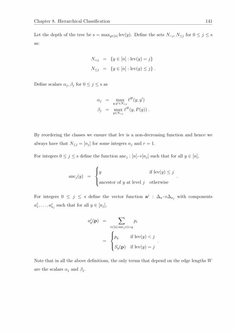
Chapter 8. Hierarchical Classification 141
Let the depth of the tree be s = maxy∈[n] lev(y). Define the sets N=j, N≤j for 0 ≤ j ≤ s
as:
N=j = y ∈ [n] : lev(y) = j
N≤j = y ∈ [n] : lev(y) ≤ j .
Define scalars αj, βj for 0 ≤ j ≤ s as
αj = maxy,y′∈N=j
`H(y, y′)
βj = maxy∈N=j
`H(y, P (y)) .
By reordering the classes we ensure that lev is a non-decreasing function and hence we
always have that N≤j = [nj] for some integers nj and r = 1.
For integers 0 ≤ j ≤ s define the function ancj : [n]→[nj] such that for all y ∈ [n],
ancj(y) =
y if lev(y) ≤ j
ancestor of y at level j otherwise
.
For integers 0 ≤ j ≤ s define the vector function aj : ∆n→∆nj with components
aj1, . . . , ajnj
such that for all y ∈ [nj],
ajy(p) =∑
i∈[n]:ancj(i)=y
pi
=
py if lev(y) < j
Sy(p) if lev(y) = j
.
Note that in all the above definitions, the only terms that depend on the edge lengths W
are the scalars αj and βj.

Chapter 8. Hierarchical Classification 142
4 5 6 7
2 3
1p1 = 0
S1(p) = 1
p2 = 0.2S2(p) = 0.3
p3 = 0S3(p) = 0.7
p4 = 0.1S4(p) = 0.1
p5 = 0S5(p) = 0
p6 = 0S6(p) = 0.1
p7 = 0.2S7(p) = 0.6
8 9p8 = 0.1
S8(p) = 0.1p9 = 0
S9(p) = 0
10 11p10 = 0.2
S10(p) = 0.2p11 = 0.2
S11(p) = 0.2
Figure 8.2: An example tree and an associated conditional probability vector p(x) forsome instance x, along with S(p(x)). The Bayes optimal prediction is shaded here.
8.3 Bayes Optimal Classifier for the Tree-Distance
Loss
In this section we characterize the Bayes optimal classifier minimizing the expected tree-
distance loss. We show that such a predictor can be viewed as a ‘greater than 12
conditional
probability subtree detector’. We then design a scheme for computing this prediction
based on this observation.
Figure 8.2 gives an illustration for Theorem 8.1 below, characterizing the Bayes optimal
classifier for the tree-distance loss.
Theorem 8.1. Let H = ([n], E,W ) and let `H : [n]× [n]→R+ be the tree-distance loss for
the tree H. Then there exists a g∗ : X→[n] such that for all x ∈ X the following holds:
(a) Sg∗(x)(p(x)) ≥ 12
(b) Sy(p(x)) ≤ 12,∀y ∈ C(g∗(x)) .
Also, g∗ is a Bayes optimal classifier for the tree-distance loss, i.e.
reg`H
D [g∗] = 0 .

Chapter 8. Hierarchical Classification 143
Proof. We shall simply show for all p ∈ ∆n, there exists a y∗ ∈ [n] such that
Sy∗(p) ≥ 1
2(8.1)
Sy(p) ≤ 1
2, ∀y ∈ C(y∗) , (8.2)
and is such that
〈p, `Hy∗〉 = miny∈[n]〈p, `Hy 〉 .
This would imply reg`H
p (y∗) = 0. The theorem then simply follows from linearity of
expectation.
Let p ∈ ∆n. We construct a y∗ ∈ [n] satisfying Equations (8.1) and (8.2) in the following
way. We start at the root node, which always satisfies Equation (8.1), and keep on moving
to the child of the current node that satisfies Equation (8.1), and terminate when we reach
a leaf node, or a node where all of its children fail Equation (8.1). Clearly the resulting
node, y∗, satisfies both Equations (8.1) and (8.2).
Now we show that y∗ indeed minimizes 〈p, `Hy 〉 over y ∈ [n].
Let y′ ∈ argmint〈p, `Ht 〉. If y′ = y∗ we are done, hence assume y′ 6= y∗.
Case 1: y′ /∈ D(y∗)
〈p, `Hy′ 〉 − 〈p, `Hy∗〉 =∑
y∈D(y∗)
py(`H(y, y′)− `H(y, y∗)) +
∑y∈[n]\D(y∗)
py(`H(y, y′)− `H(y, y∗))
=∑
y∈D(y∗)
py(`H(y∗, y′)) +
∑y∈[n]\D(y∗)
py(`H(y, y′)− `H(y, y∗))
≥∑
y∈D(y∗)
py(`H(y∗, y′)) +
∑y∈[n]\D(y∗)
py(−`H(y′, y∗)))
= `H(y′, y∗)(2Sy∗(p)− 1)
≥ 0
Case 2: y′ ∈ D(y∗) \ C(y∗)
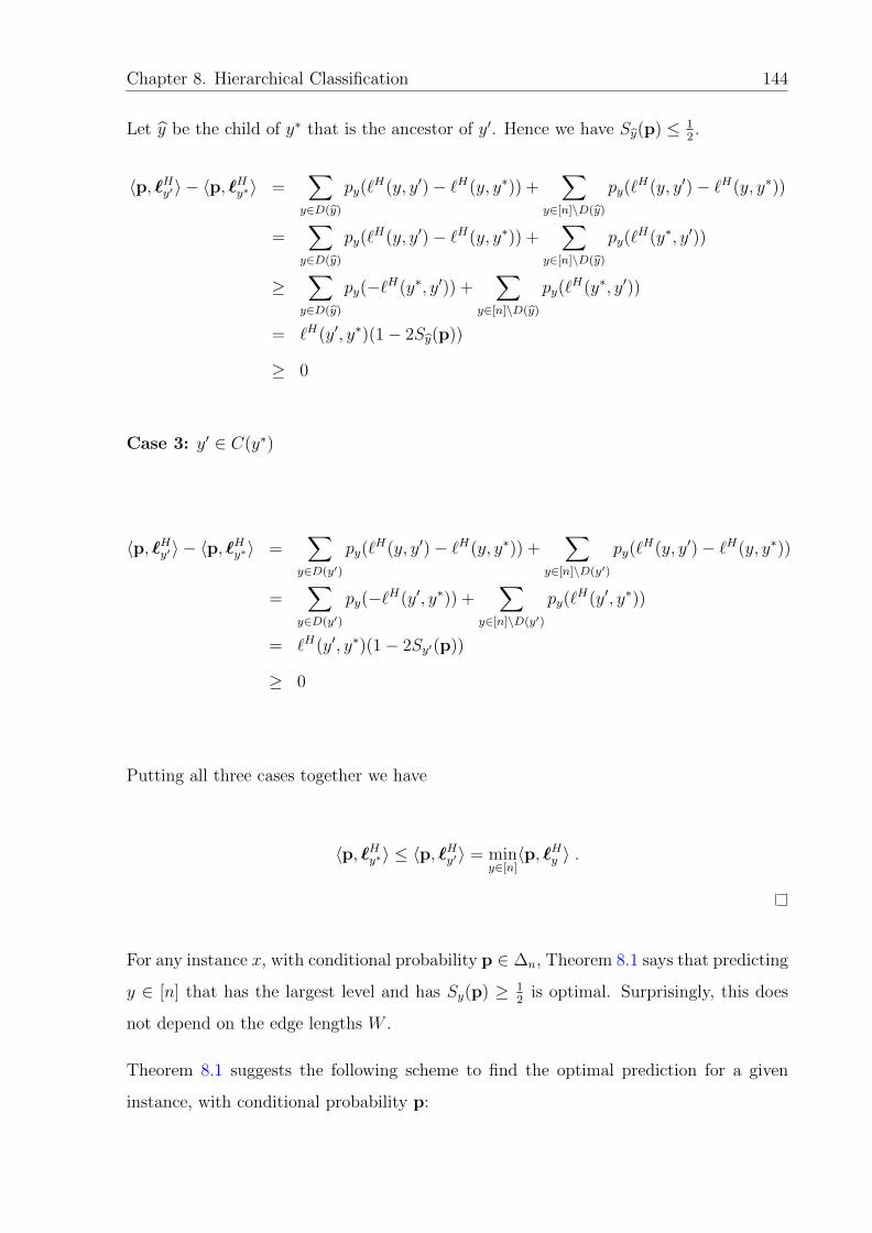
Chapter 8. Hierarchical Classification 144
Let y be the child of y∗ that is the ancestor of y′. Hence we have Sy(p) ≤ 12.
〈p, `Hy′ 〉 − 〈p, `Hy∗〉 =∑
y∈D(y)
py(`H(y, y′)− `H(y, y∗)) +
∑y∈[n]\D(y)
py(`H(y, y′)− `H(y, y∗))
=∑
y∈D(y)
py(`H(y, y′)− `H(y, y∗)) +
∑y∈[n]\D(y)
py(`H(y∗, y′))
≥∑
y∈D(y)
py(−`H(y∗, y′)) +∑
y∈[n]\D(y)
py(`H(y∗, y′))
= `H(y′, y∗)(1− 2Sy(p))
≥ 0
Case 3: y′ ∈ C(y∗)
〈p, `Hy′ 〉 − 〈p, `Hy∗〉 =∑
y∈D(y′)
py(`H(y, y′)− `H(y, y∗)) +
∑y∈[n]\D(y′)
py(`H(y, y′)− `H(y, y∗))
=∑
y∈D(y′)
py(−`H(y′, y∗)) +∑
y∈[n]\D(y′)
py(`H(y′, y∗))
= `H(y′, y∗)(1− 2Sy′(p))
≥ 0
Putting all three cases together we have
〈p, `Hy∗〉 ≤ 〈p, `Hy′ 〉 = miny∈[n]〈p, `Hy 〉 .
For any instance x, with conditional probability p ∈ ∆n, Theorem 8.1 says that predicting
y ∈ [n] that has the largest level and has Sy(p) ≥ 12
is optimal. Surprisingly, this does
not depend on the edge lengths W .
Theorem 8.1 suggests the following scheme to find the optimal prediction for a given
instance, with conditional probability p:

Chapter 8. Hierarchical Classification 145
1. For each j ∈ 1, 2, . . . , s create a multiclass problem instance with the classes being
elements of N≤j = [nj], and the probability associated with each class in y ∈ N≤jis equal to ajy(p), i.e. py if lev(y) < j and equal to Sy(p) if lev(y) = j.
2. For each multiclass problem j ∈ 1, 2, . . . , s, if there exists a class with probability
mass at least 12
assign it to v∗j , otherwise let v∗j = ⊥.
3. Find the largest j such that v∗j 6= ⊥ and return the corresponding v∗j , or return the
root 1 if v∗j = ⊥ for all j ∈ [s].
We will illustrate the above procedure for the example in Figure 8.2.
Example 8.1. From Figure 8.2 we have that s = 3. The three induced multiclass problems
are given below.
1. n1 = 3, and the class probabilities are given as 110
[0, 3, 7]. Clearly, v∗1 = 3.
2. n2 = 7, and the class probabilities are given as 110
[0, 2, 0, 1, 0, 1, 6]. Clearly v∗2 = 7.
3. n3 = 11, and the class probabilities are given as 110
[0, 2, 0, 1, 0, 0, 2, 1, 0, 2, 2]. Clearly,
v∗3 = ⊥.
And hence the largest j such that v∗j 6= ⊥ is 2, and the scheme returns v∗2 = 7.
The reason such a scheme as the one above is of interest to us, is that the second step in
the above scheme exactly corresponds to the Bayes optimal classifier for the abstain(12)
loss employed in the problem of multiclass classification with an abstain option as given
in Chapter 7, Equation (7.2).
8.4 Cascade Surrogate for Hierarchical Classification
In this section we construct a template surrogate ψC and template predictor predC based
on the scheme in Section 8.3 and is constituted of simpler surrogates ψj and predictors
predj. We then give a excess risk bound relating ψC and `H assuming the existence of

Chapter 8. Hierarchical Classification 146
excess risk bounds relating the component surrogates ψj and the abstain(12) loss. We
shall denote the abstain(12) loss with nj classes as `?,nj in this chapter.
For all j ∈ 1, 2, . . . , s, let the surrogate ψj : [nj] × Rdj→R+ and predictor predj :
Rdj→([nj] ∪ ⊥) be such that they are calibrated w.r.t. `?,nj for some integers dj. Let
d =∑j
i=1 dj. Let any u ∈ Rd be decomposed as u = [u>1 , . . . ,u>s ]>, with each uj ∈ Rdj .
The template surrogate, that we call the cascade surrogate ψC : [n]×Rd→R+, is defined
in terms of its constituent surrogates as follows:
ψC(y,u) =s∑
j=1
ψj(ancj(y),uj) . (8.3)
The template predictor, predC, is defined via the function predCj : Rd1 × . . . × Rdj→[nj]
which is defined recursively as follows:
predCj (u1, . . . ,uj) =
predj(uj) if predj(uj) 6= ⊥
predCj−1(u1, . . . ,uj−1) otherwise
(8.4)
The function predC0 takes no arguments and simply returns 1 (the root node). Occasion-
ally we abuse notation by representing predCj (u1, . . . ,uj) simply as predC
j (u).
The template predictor, predC : Rd→[n] is simply defined as predC(u) = predCs (u1, . . . ,us) .
The lemma below, captures the essence of the reduction from the problem of hierarchical
classification to the problem of multiclass classification with an abstain option.
Lemma 8.2. For all p ∈ ∆n,u ∈ Rd we have
reg`H
p (predC(u)) ≤s∑
j=1
γj(uj) · reg`?,nj
aj(p)(predj(uj)),
where γj(uj) =
2αj if predj(uj) 6= ⊥
2βj if predj(uj) = ⊥.
Proof. For all 0 ≤ j ≤ s, define `H,j : [nj] × [nj]→R+ as simply the restriction of `H to
[nj]× [nj].

Chapter 8. Hierarchical Classification 147
For all j ∈ [s], we will first prove a bound relating the tree-distance regret at level j, with
the tree-distance regret at level j − 1 and abstain loss regret at level j as follows:
reg`H,j
aj(p)(predCj (u)) ≤ reg`
H,j−1
aj−1(p)(predCj−1(u)) + γj(uj) · reg`
?,nj
aj(p)(predj(uj)) .
The theorem would simply follow from applying such a bound recursively and observing
that reg`H,0
a0(p)(predC0 (u)) = 0.
One observation of the tree-distance loss that will be often of use in the proof is that for
all non-root y ∈ [n]
`H(y, y′)− `H(P (y), y′) =
−`H(y, P (y)) if y′ ∈ D(y)
`H(y, P (y)) otherwise
The details of the proof follows: Fix j ∈ [s],u ∈ Rd,p ∈ ∆n.
Let y∗j = argminy∈[nj ]reg`
H,j
aj(p)(y).
Case 1: predj(uj) 6= ⊥
reg`H,j
aj(p)(predCj (u)) =
nj∑y=1
ajy(p)(`H(y, predCj (u))− `H(y, y∗j ))
≤ `H(y∗j , predCj (u))(1− 2aj
predCj (u)
(p)) (8.5)
We also have,
reg`?,nj
aj(p)(predj(uj)) = 1− ajpredj(uj)(p)− min
y∈[nj ]∪⊥〈aj(p), `?,nj
y 〉
≥ 1− ajpredj(uj)(p)− 〈aj(p), `
?,nj⊥ 〉
=1
2− ajpredj(uj)
(p)
=1
2− aj
predCj (u)
(p) . (8.6)
The last inequality above follows because if predj(uj) 6= ⊥, then predCj (u) = predj(uj).

Chapter 8. Hierarchical Classification 148
Putting Equations (8.5) and (8.6) together, we get
reg`H,j
aj(p)(predCj (u)) ≤ 2`H(y∗j , predC
j (u)) · reg`?,nj
aj(p)(predj(uj))
≤ 2αj · reg`?,nj
aj(p)(predj(uj)) (8.7)
Case 2: predj(uj) = ⊥
In this case predCj (u) = predC
j−1(u), and hence lev(predCj (u)) ≤ j − 1.
We now have,
〈aj(p), `H,jpredC
j (u)〉 − 〈aj−1(p), `H,j−1
predCj−1(u)
〉
= 〈aj(p), `H,jpredC
j (u)〉 − 〈aj−1(p), `H,j−1
predCj (u)〉
=∑y∈N=j
Sy(p)(`H(y, predC
j (u))− `H(P (y), predCj (u))
)=
∑y∈N=j
Sy(p)`H(y, P (y)) (8.8)
For ease of analysis, we divide case 2, further into two sub-cases.
Case 2a: lev(y∗j ) < j
〈aj−1(p), `H,j−1y∗j−1
〉 − 〈aj(p), `H,jy∗j〉 = 〈aj−1(p), `H,j−1
y∗j−1〉 − 〈aj−1(p), `H,j−1
y∗j〉
+〈aj−1(p), `H,j−1y∗j
〉 − 〈aj(p), `H,jy∗j〉
≤ 〈aj−1(p), `H,j−1y∗j
〉 − 〈aj(p), `H,jy∗j〉
=∑y∈N=j
Sy(p)(`H(P (y), y∗j )− `H(y, y∗j ))
=∑y∈N=j
Sy(p)(−`H(y, P (y))) (8.9)
Adding, Equation (8.8) and (8.9), we get
reg`H,j
aj(p)(predCj (u)) ≤ reg`
H,j−1
aj−1(p)(predCj−1(u)) (8.10)
Case 2b: lev(y∗j ) = j

Chapter 8. Hierarchical Classification 149
For any integers a, b with a ≤ b and vector v ∈ Rb let v∣∣1:a∈ Ra be the vector given by
the first a components of v.
〈aj−1(p), `H,j−1y∗j−1
〉 − 〈aj−1(p), `Hy∗j
∣∣[1:nj−1]
〉 ≤ 〈aj−1(p), `H,j−1P (y∗j ) 〉 − 〈aj−1(p), `Hy∗j
∣∣[1:nj−1]
〉
=∑
y∈N≤j−1
aj−1y (p)(`H(y, P (y∗j ))− `H(y, y∗j ))
=∑
y∈N≤j−1
aj−1y (p)(−`H(y∗j , P (y∗j )))
= −`H(y∗j , P (y∗j )) (8.11)
Also,
〈aj−1(p), `Hy∗j
∣∣[1:nj−1]
〉 − 〈aj(p), `H,jy∗j〉
=∑y∈N=j
Sy(p)(`H(P (y), y∗j )− `H(y, y∗j ))
=∑
y∈N=j\y∗j Sy(p)(−`H(y, P (y))) + Sy∗j (p)(`H(y∗j , P (y∗j ))) . (8.12)
Adding Equations (8.8), (8.11) and (8.12), we get
reg`H,j
aj(p)(predCj (u)) ≤ reg`
H,j−1
aj−1(p)(predCj−1(u)) + (2Sy∗j (p)− 1) · `H(y∗j , P (y∗j ))
≤ reg`H,j−1
aj−1(p)(predCj−1(u)) + (2Sy∗j (p)− 1) · βj . (8.13)
Inequality (8.13) follows because, by the definitions of y∗j and Theorem 8.1 we have that
Sy∗j (p) ≥ 12.

Chapter 8. Hierarchical Classification 150
Also, we have that
reg`?,nj
aj(p)(predj(uj)) = reg`?,nj
aj(p)(⊥)
=1
2− min
y∈[n]∪⊥〈aj(p), `?,nj
y 〉
≥ 1
2− 〈aj(p), `
?,njy∗j〉
=1
2− (1− Sy∗j (p))
= Sy∗j (p)− 1
2. (8.14)
Putting Equations (8.13) and (8.14) together, we have that
reg`H,j
aj(p)(predCj (u)) ≤ reg`
H,j−1
aj−1(p)(predCj−1(u)) + 2βj · reg`
?,nj
aj(p)(predj(uj)). (8.15)
Putting the results for case 1, case 2a and case 2b, from Equations (8.7), (8.10) and (8.15)
respectively, we have
reg`H,j
aj(p)(predCj (u)) ≤ reg`
H,j−1
aj−1(p)(predCj−1(u)) + γj(uj) · reg`
?,nj
aj(p)(predj(uj)) .
Lemma 8.2 bounds the `H regret on a distribution D, by a weighted sum of abstain loss
regrets, each over a modified distribution derived from D. Each of the components of
the surrogate ψC is exactly designed to minimize the abstain loss for the corresponding
modified distribution. Assuming an excess risk bound relating ψj and `?,nj for all j ∈ [s],
one can easily derive an excess risk bound relating `H and ψC. This is done in the theorem
below.
Theorem 8.3. For all j ∈ [s], let ψj : [nj]× Rdj and predj : Rdj→nj be such that for all
fj : X→Rdj , and all distributions D over X × [nj] we have
reg`?,nj
D [predj fj] ≤ C · regψj
D [fj],

Chapter 8. Hierarchical Classification 151
for some constant C > 0. Then for all f : X→Rd and distributions D over X × [n],
reg`H
D [predC f ] ≤ 2αhC · regψC
D [f ] .
Proof. Fix u ∈ Rd,p ∈ ∆n. From Lemma 8.2 and the observation that γj(uj) ≤ αj, we
have that
reg`H
p (predC(u)) ≤s∑
j=1
2αj · reg`?,nj
aj(p)(predj(uj))
≤ 2αh ·s∑
j=1
·reg`?,nj
aj(p)(predj(uj))
≤ 2αhC ·s∑
j=1
regψj
aj(p)(uj)
= 2αhC · regψC
p (u) .
The proof now simply follows from linearity of expectation.
Thus, one just needs to plug in appropriate convex surrogates ψj and predictors predj to
get concrete calibrated surrogates for hierarchical classification. The results of Chapter
7 can be used to immediately get three such by setting the component surrogates ψj
and predictors predj as either the CS, OVA or BEP surrogates and predictors. We call
the resulting algorithms (surrogates and predictors) as CS-cascade , OVA-cascade and
BEP-cascade.
An interesting consequence of the BEP-cascade being calibrated w.r.t. `H is that
CCdim(`H) ≤ s · dlog2(n)e ,
which for balanced trees is of the order of (log(n))2. Disappointingly though, the BEP-
cascade algorithm does not work as well as OVA-cascade and CS-cascade, with parametric
function classes like the linear function class, on real data sets.

Chapter 8. Hierarchical Classification 152
Algorithm 2 OVA-Cascade Training
Input: S = ((x1, y1), . . . , (xM , yM)) ∈ (X × [n])M , H = ([n], E).Parameters: Regularization parameter C > 0
for i = 1 : nLet tj = 2 · 1(yj ∈ D(i))− 1, ∀j ∈ [M ]Ti = ((x1, t1), . . . , (xM , tM)) ∈ (X × +1,−1)M .fi=SVM-Train(Ti, C)Let t′j = 2 · 1(yj = i)− 1, ∀j ∈ [M ]T ′i = ((x1, t
′1), . . . , (xM , t
′M)) ∈ (X × +1,−1)M .
f ′i=SVM-Train(T ′i , C)end for
8.5 OVA-Cascade Algorithm
In this section, we will consider the OVA cascade in more detail, as the problem of opti-
mizing the OVA-cascade surrogate is very amenable to being broken down into multiple
separate binary SVM problems, and thus can be easily parallelized. Also, there are nu-
merous efficient solvers for binary SVM, removing the need to tailor a generic convex
optimization algorithm to suit our purpose.
To make the dependence on the number of classes more explicit, we shall use ψOVA,n and
predOVA,nτ , to denote the OVA surrogate and predictor with n classes and threshold τ as
in Section 7.4.
Let ψj = ψOVA,nj and predj = predOVA,njτj
for some τj ∈ (−1, 1). In this case we have
dj = nj. In the surrogate minimizing algorithm for OVA-cascade, one solves s one-vs-all
SVM problems. Problem j has nj classes, with the classes corresponding to the nj−1 nodes
in the hierarchy at level less than j, and nj − nj−1 ‘super-nodes’ in the hierarchy at level
j which also absorb the nodes of its descendants. The resulting training and prediction
algorithms can thus be simplified and they are presented in Algorithms 2 and 3. The
training phase requires an SVM optimization sub-routine, SVM-Train, which takes in a
binary dataset and a regularization parameter C and returns a real valued function over
the instance space minimizing the regularized hinge loss over an appropriate function
space.
Theorems 7.3 and 8.3 immediately give the following excess risk bound for OVA-cascade.

Chapter 8. Hierarchical Classification 153
Algorithm 3 OVA-Cascade Prediction
Input: x ∈ X , H = ([n], E), trained models fi, f′i for all i ∈ [n]
Parameters: Scalars τ1, . . . , τs in (−1, 1)
for j = s down to 1Construct u ∈ Rnj such that, for all i ∈ [nj],
ui =
fi(x) if lev(i) = j
f ′i(x) if lev(i) < j
if maxi ui > τjreturn argmaxi ui
end ifend forreturn 1
Corollary 8.4. For 1 ≤ j ≤ s, let τj ∈ (−1, 1). Let the component surrogates and
predictors of ψC and predC be ψj = ψOVA,nj and predj = predOVA,njτj
. Then, for all
distributions D and functions f : X→Rd,
reg`H
D [predC f ] ≤ αh1−maxj |τj|
· regψC
D [f ]
To get the best bound from Corollary 8.4, one must set τj = 0 for all j ∈ [s]. However,
using a slightly more intricate version of Theorem 7.3 and the full extent of Lemma 8.2,
one can give a better upper bound for the `H-regret than in Corollary 8.4, and this tighter
upper bound is minimized for a different τj. This observation is captured by Theorem
8.5 below.
Theorem 8.5. For 1 ≤ j ≤ s, let τj =αj−βjαj+βj
. Let the component surrogates and predictors
of ψC and predC be ψj = ψOVA,nj and predj = predOVA,njτj
. Then, for all distributions D
and functions f : X→Rd,
reg`H
D [predC f ] ≤ 1
2maxj∈[s]
(αj + βj) · regψC
D [f ]
To prove the above theorem we first give the more intricate version of Theorem 7.3, whose
proof still follows from the proof of Theorem 7.3.

Chapter 8. Hierarchical Classification 154
Lemma 8.6. Let τ ∈ (−1, 1). For all u ∈ Rn,p ∈ ∆n. Then for all p ∈ ∆n
reg`?,n
p (predOVA,nτ (u)) ≤
(1(predOVA,n(u) = ⊥)
2(1− τ)+
1(predOVA,n(u) 6= ⊥)
2(1 + τ)
)· regψ
OVA,n
p (u) .
Proof. (Proof of Theorem 8.5)
Let u ∈ Rd,p ∈ ∆n, From Lemmas 8.2 and 8.6, we have that
reg`H
p (predC(u))
≤h∑j=1
γj(uj) · reg`?,nj
aj(p)(predj(uj))
≤h∑j=1
γj(uj)
(1(predOVA,nj(uj) = ⊥)
2(1− τj)+
1(predOVA,nj(uj) 6= ⊥)
2(1 + τj)
)· regψ
OVA,nj
aj(p)(uj)
=h∑j=1
(βj · 1(predOVA,nj(uj) = ⊥)
(1− τj)+αj · 1(predOVA,nj(uj) 6= ⊥)
(1 + τj)
)· regψ
OVA,nj
aj(p)(uj)
For each j ∈ [h], the coefficients of both the terms within parantheses (i.e.αj
1+τjand
βj1−τj )
both evaluate toαj+βj
2when the thresholds τj are set as τj =
αj−βjαj+βj
. In fact it can easily
be seen that this value of τj minimizes the worst-case coefficient of regψOVA,nj
aj(p)(uj) in the
bound. Thus, we have
reg`H
p (predC(u)) ≤h∑j=1
1
2(αj + βj) · regψ
OVA,nj
aj(p)(uj)
≤ 1
2maxj∈[h]
(αj + βj) ·h∑j=1
regψOVA,nj
aj(p)(uj)
=1
2maxj∈[h]
(αj + βj) · regψC
p (u) .
The Theorem now follows from linearity of expectation.
One can clearly see the effect of improved bounds given by setting τj as in Theorem 8.5
for the unweighted hierarchy, in which case αj = 2j and βj = 1.
Corollary 8.7. Let the hierarchy H be an unweighted tree with all edges having length
1. Let the component surrogates and predictors of ψC and predC be ψj = ψOVA,nj and
predj = predOVA,njτj
.

Chapter 8. Hierarchical Classification 155
a. For all j ∈ [s] let τj = 0, then, for all distributions D and functions f : X→Rd,
reg`H
D [predC f ] ≤ 2s · regψC
D [f ] .
b. For all j ∈ [s] let τj = 2j−12j+1
, then, for all distributions D and functions f : X→Rd,
reg`H
D [predC f ] ≤(
s +1
2
)· regψ
C
D [f ] .
Thus setting τj = 2j−12j+1
gives almost a factor 2 improvement over setting τj = 0. This
threshold setting is also intuitively satisfying, as it says to use a higher threshold and
predict conservatively (abstain more often) in deeper levels, and use a lower threshold to
predict aggressively in levels nearer to the root. In practice, the optimal thresholds are
distribution dependent and are best obtained via cross-validation.
8.6 Experiments
We run our cascade surrogate based algorithm for hierarchical classification on some stan-
dard document classification tasks with a class hierarchy and compare the results against
other standard algorithms. We use the unweighted tree-distance loss as the evaluation
metric. The details of the datasets and the algorithms are given below.
8.6.1 Datasets
We used several standard multiclass document classification datasets, all of which have
one class label per example. The basic statistics of the datasets is given in Table 8.1.
• CLEF [32] Hierarchical collection of medical images.
• IPC 1 Patents organized according to the International Patent Classification Hier-
archy.
1http://www.wipo.int/classifications/ipc/en/support/
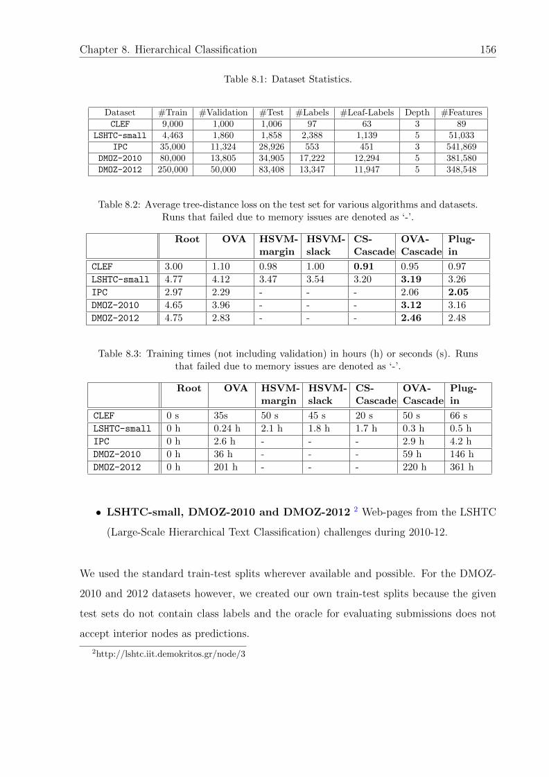
Chapter 8. Hierarchical Classification 156
Table 8.1: Dataset Statistics.
Dataset #Train #Validation #Test #Labels #Leaf-Labels Depth #FeaturesCLEF 9,000 1,000 1,006 97 63 3 89
LSHTC-small 4,463 1,860 1,858 2,388 1,139 5 51,033IPC 35,000 11,324 28,926 553 451 3 541,869
DMOZ-2010 80,000 13,805 34,905 17,222 12,294 5 381,580DMOZ-2012 250,000 50,000 83,408 13,347 11,947 5 348,548
Table 8.2: Average tree-distance loss on the test set for various algorithms and datasets.Runs that failed due to memory issues are denoted as ‘-’.
Root OVA HSVM-margin
HSVM-slack
CS-Cascade
OVA-Cascade
Plug-in
CLEF 3.00 1.10 0.98 1.00 0.91 0.95 0.97
LSHTC-small 4.77 4.12 3.47 3.54 3.20 3.19 3.26
IPC 2.97 2.29 - - - 2.06 2.05
DMOZ-2010 4.65 3.96 - - - 3.12 3.16
DMOZ-2012 4.75 2.83 - - - 2.46 2.48
Table 8.3: Training times (not including validation) in hours (h) or seconds (s). Runsthat failed due to memory issues are denoted as ‘-’.
Root OVA HSVM-margin
HSVM-slack
CS-Cascade
OVA-Cascade
Plug-in
CLEF 0 s 35s 50 s 45 s 20 s 50 s 66 s
LSHTC-small 0 h 0.24 h 2.1 h 1.8 h 1.7 h 0.3 h 0.5 h
IPC 0 h 2.6 h - - - 2.9 h 4.2 h
DMOZ-2010 0 h 36 h - - - 59 h 146 h
DMOZ-2012 0 h 201 h - - - 220 h 361 h
• LSHTC-small, DMOZ-2010 and DMOZ-2012 2 Web-pages from the LSHTC
(Large-Scale Hierarchical Text Classification) challenges during 2010-12.
We used the standard train-test splits wherever available and possible. For the DMOZ-
2010 and 2012 datasets however, we created our own train-test splits because the given
test sets do not contain class labels and the oracle for evaluating submissions does not
accept interior nodes as predictions.
2http://lshtc.iit.demokritos.gr/node/3
Chapter 8. Hierarchical Classification 157
8.6.2 Algorithms
We run a variety of algorithms on the above datasets. The details of the algorithms are
given below.
Root: This is a simple baseline method where the returned classifier always predicts
the root of the hierarchy.
OVA: This is the standard one-vs-all SVM algorithm which completely ignores the
hierarchy information and treats the problem as one of standard multiclass classification.
HSVM-margin and HSVM-slack : These algorithms are Struct-SVM like [101] al-
gorithms for the tree-distance loss as proposed in Cai and Hoffman [16]. HSVM-margin
uses margin rescaling, while HSVM-slack uses slack rescaling and are considered among
the state-of-the-art algorithms for hierarchical classification.
OVA-Cascade: This is the algorithm in which we minimize the surrogate ψC with the
component surrogates being ψj = ψOVA,nj and is detailed as Algorithms 2 and 3. All
the datasets in Table 8.1 have the property that all instances are associated only with a
leaf-label (note however that we can still predict interior nodes), and hence the step of
computing f ′i in Algorithm 2 can be skipped, and f ′i can be set to be identically equal to
negative infinity for all i ∈ [n]. Note that, in this case, the training phase is very similar
to the ‘less-inclusive policy’ using the ‘local node approach’ [92]. We use LIBLINEAR
[35] for the SVM-train subroutine and use the simple linear kernel. The regularization
parameter C is chosen via a separate validation set. The thresholds τj for j ∈ [s] are also
chosen via a coarse grid search using the validation set.
Plug-in classifier: This algorithm is based on estimating the conditional probabilities
using a logistic loss. Specifically, it estimates Sy(p) for all non-root nodes y. This is
done by creating a binary dataset for each y, with instances having labels which are
the descendants of y being positive and the rest being negative, and running a logistic
regression algorithm on this dataset. The final predictor is simply based on Theorem 8.1,
it chooses the deepest node y such that the estimated value of Sy(p) is greater than 12.

Chapter 8. Hierarchical Classification 158
CS-Cascade: This algorithm also minimizes the cascade surrogate ψC, but with the
component surrogates ψj being the Crammer-Singer surrogate. Using the results from
Chapter 7, one can derive excess risk transforms for the resulting cascade surrogate as
well. As all instances have labels which are leaf nodes, the s subproblems all turn out to be
multiclass learning problems with nj classes for each of which we use the Crammer-Singer
algorithm. We optimize the Crammer-Singer surrogate over the standard multiclass lin-
ear function class using the LIBLINEAR [35] software. Once again, we use the same
regularization parameter C for all the s problems, which we choose using the validation
set. We also use a threshold vector tuned on the validation set over a coarse grid.
The three algorithms, OVA-Cascade, Probability estimation, and CS-cascade are all mo-
tivated by our analysis and would form consistent algorithms for the tree-distance loss, if
used with an appropriate function class.
8.6.3 Discussion of Results
Table 8.2 gives the average tree-distance loss incurred by various algorithms on some
standard datasets, and Table 8.3 gives the times taken for running these algorithms on a
4-core CPU.3 Some of the algorithms like HSVM, and CS-cascade could not be run on the
larger datasets due to memory issues. On the smaller datasets of CLEF and LSHTC-small
where all the algorithms could be run, the algorithms motivated by our analysis – OVA-
cascade, Plug-in and CS-cascade – perform the best. On the bigger datasets, only the
OVA-cascade, plug-in and the flat OVA algorithms could be run, and both OVA-cascade
and Plug-in perform significantly better than the flat OVA. While both OVA-cascade
and Plug-in give comparable error performance, the OVA-cascade only takes about half
as much time as the Plug-in and hence is more preferable.
3HSVM, and CS-cascade effectively only use a single core due to lack of parallelization.

Part III
Complex Multiclass
Evaluation Metrics

Chapter 9
Consistent Algorithms for Complex
Multiclass Penalties
In many practical applications of machine learning, the evaluation metric used to measure
the performance of a classifier takes a complex form, and is not simply the expectation
or sum of a loss on individual examples. Indeed, this is the case with the G-mean, H-
mean and Q-mean losses used in class imbalance settings [56, 58, 63, 98, 108], the micro
and macro F1 measures used in information retrieval (IR) applications [65], the min-
max measure used in detection theory [104], and many others. The loss-matrix based
evaluation metrics, which we have studied in the previous chapters, are simply linear
functions of the confusion matrix of a classifier, while these complex evaluation metrics
are defined by more general functions of the confusion matrix.
There has been much interest in designing algorithms for such complex evaluation metrics.
A prominent example is the SVMperf algorithm [53], which was developed primarily for
the binary setting; other examples include algorithms for the binary F1-measure and
its multiclass and multilabel variants [30, 31, 70, 74–76, 113]. More recently, there has
been increasing interest in designing consistent algorithms for complex evaluation metrics;
however, most of this work has focused on the binary case [61, 69, 71, 113].
In the case of loss-matrix based evaluation metrics, one can always design consistent
algorithms by minimizing the n-dimensional convex calibrated conditional probability
160

Chapter 9. Complex Multiclass Penalties 161
estimation surrogate of Theorem 5.1 or Lemma 4.1. But for these complex evaluation
metrics, these methods do not apply.
In this chapter we address the problem of designing consistent algorithms for such com-
plex evaluation metrics. Our approach involves viewing the learning problem as an opti-
mization problem over the set of feasible confusion matrices, and solving (approximately,
based on the training sample) this optimization problem using an appropriate optimiza-
tion method. In particular, we design an algorithm that we call the Bayes-Frank-Wolfe
algorithm, and show that the resulting algorithm is consistent for convex evaluation met-
rics, which includes many complex evaluation metrics used in practice, as seen in Table
9.1.
9.1 Chapter Organization
We begin by formally defining the notion of a complex multiclass penalty, and give several
examples in Section 9.2. We then study the notion of consistency for such complex
penalties, and make some observations linking it to optimization in Section 9.3. Building
on the connection to optimization, we give the Bayes-Frank-Wolfe algorithm in Section
9.4, which is based on the Frank-Wolfe algorithm in optimization, and show that it forms
a consistent learning algorithm for a large family of such complex penalties.
9.2 Complex Multiclass Penalties
The problem is set in the standard supervised learning setting, as detailed in Section 2.2,
with one major difference. Instead of considering just classifiers h : X→Y , we consider
randomized classifiers h, which give a random variable taking values in Y , for an input
x ∈ X . We represent such a classifier by a function h : X→∆Y , i.e. h(x) is distributed as
h(x) for all x ∈ X . This is a strictly more general setting, and we show that this generality
is indeed required for complex losses. For the sake of simplicity, we set Y = Y = [n] in this
chapter, the results can be trivially extended for any finite label space Y and prediction
space Y .

Chapter 9. Complex Multiclass Penalties 162
The evaluation metrics in this chapter depend on the confusion matrix of a classifier.
The confusion matrix of a classifier h : X→∆n w.r.t. a distribution D, is denoted by
CD[h] ∈ [0, 1]n×n, and has entries given by
CDi,j[h] = P
(Y = i, h(X) = j
),
where the probability is over the randomness in X, Y and also the classifier h, which is
such that h(x) ∼ h(x).
Clearly,
n∑j=1
CDi,j[h] = P(Y = i) ,
n∑i=1
CDi,j[h] = hj(x) = P(h(X) = j) .
For a given distribution D, we denote the set of all matrices satisfying the first constraint
as CD, i.e.
CD =
C ∈ [0, 1]n×n :
n∑j=1
Ci,j = P(X,Y )∼D(Y = i), ∀i ∈ [n]
.
We will be interested in general, complex evaluation metrics that can be expressed as
an arbitrary function of the entries of the confusion matrix CD[h]. For any continuous
penalty function ϕ : [0, 1]n×n→R+, define the ϕ-risk of h w.r.t. D as follows
LϕD[h] = ϕ(CD[h]) .
The ϕ-risk defined above is exactly analogous to the `-risk defined for a loss matrix ` in
Chapter 2.
As the following examples show, this formulation captures both common loss-matrix based
evaluation metrics studied in previous chapters, which are effectively linear functions of
the entries of the confusion matrix, and more complex evaluation metrics such as the

Chapter 9. Complex Multiclass Penalties 163
G-mean, micro F1-measure, and several others.1
Example 9.1 (Loss-matrix based evaluation metrics). Consider a multiclass loss ` : Y ×Y→R+ with loss matrix matrix L ∈ Rn×n
+ , as in previous chapters. Let the penalty
function ϕ : [0, 1]n×n→R+, be such that
ϕ(C) = 〈L,C〉 .
Then the ϕ-risk is such that for any classifier h : X→∆n,
LϕD[h] = 〈L,CD[h]〉
=n∑i=1
n∑j=1
Li,jE[1(Y = i)1(h(X) = j)
]= E
[LY,h(X)
]= Eh
[er`D[h]
],
where once again h(x) ∼ h(x) for all x ∈ X .
Hence we have that the loss-matrix based evaluation metrics correspond to using penalties
that are a linear function of the confusion matrix.
Example 9.2 (Binary evaluation metrics). In the binary setting, where n = 2 and the
labels are often indexed as Y = −1, 1, the confusion matrix of a classifier contains
the proportions of true negatives (C−1,−1 = TN), false positives (C−1,1 = FP), false
negatives (C1,−1 = FN), and true positives (C1,1 = TP). Our framework thus includes
any evaluation metric expressed in terms of these 4 quantities in binary classification.
For example, the Fβ-measure (β > 0) given by the penalty function,
ϕFβ(C) = 1− (1 + β2) TP
(1 + β2) TP + β2 FN + FP,
all ‘ratio-of-linear’ binary evaluation metrics [61], and more generally, all ‘non-decomposable’
binary evaluation metrics [71].
1Many of these evaluation metrics are given as gains in their original form, and hence we subtractthem from a constant to consider them as penalties.

Chapter 9. Complex Multiclass Penalties 164
Example 9.3 (A-mean evaluation metric). The arithmetic mean evaluation metric is a
simple evaluation metric that balances the errors from all classes [69] and is given by the
penalty function,
ϕAM(C) =n∑i=1
(∑n
j=1Ci,j)− Ci,i∑nj=1Ci,j
.
Example 9.4 (G-mean evaluation metric). The geometric mean evaluation metric is used
to evaluate both binary and multiclass classifiers in settings with class imbalance [98, 108],
and is given by the penalty function
ϕGM(C) = 1−( n∏
i=1
Ci,i∑nj=1Ci,j
)1/n
.
Example 9.5 (H-mean evaluation metric). The harmonic mean evaluation metric is de-
signed for situations with class imbalance [56], and is given by the penalty function
ϕHM(C) = 1− n(
n∑i=1
∑nj=1Ci,j
Ci,i
)−1
.
Example 9.6 (Q-mean evaluation metric). The Q-mean evaluation metric [63], is another
evaluation metric designed for problems with class imbalance and is given by the penalty
function
ϕQM(C) =
√√√√ 1
n
n∑i=1
(1− Ci,i∑n
j=1Ci,j
)2
.
Other examples of complex evaluation metrics include the macro F1-measure [65], the
spectral norm measure [59, 67, 78], and the min-max measure in detection theory [104];
see Table 9.1.
The ultimate goal in the learning problem with a complex penalty ϕ : [0, 1]n×n→R+, is
to find a classifier that achieves as small a ϕ-risk as possible. In this context one can
define the minimum ϕ-risk, ϕ-regret and consistency w.r.t. ϕ, in a manner similar to
such notions defined for a loss matrix ` in Chapter 2.
The minimum ϕ-risk Lϕ,∗D is defined as
Lϕ,∗D = infh:X→∆n
LϕD[h] ,

Chapter 9. Complex Multiclass Penalties 165
Table 9.1: Examples of complex multiclass evaluation metrics.
Evaluation metric ϕ(C) Convex over CD?
A-Mean∑n
i=1
(∑nj=1 Ci,j)−Ci,i∑n
j=1 Ci,jYes
G-mean 1−(∏n
i=1Ci,i∑nj=1 Ci,j
)1/n
Yes
H-mean 1− n(∑n
i=1
∑nj=1 Ci,j
Ci,i
)−1
Yes
Q-mean
√1n
∑ni=1
(1− Ci,i∑n
j=1 Ci,j
)2
No
Micro F1 1− 2∑ni=2 Ci,i
2−∑ni=1 C1i−
∑ni=1 Ci1
No
Macro F1 1− 1n
∑ni=1
2Ci,i∑nj=1 Ci,j +
∑nj=1 Cji
Yes
Spectral norm 1− ‖C‖∗ Yes
(where C is obtained from C
by normalizing rows to sum to 1
and setting diagonal entries to 0)
Min-max 1−mini∈[n]Ci,i∑nj=1 Ci,j
Yes
and the ϕ-regret of a classifier h : X→∆n is given as
regϕD[h] = LϕD[h]− Lϕ,∗D .
Definition 9.1 (ϕ-consistency). An algorithm that takes a training sample S ∈ (X ×Y)M
drawn i.i.d from D and returns a classifier hM (which is a random variable depending on
S) is said to be consistent w.r.t. ϕ, or simply ϕ-consistent, if as M approaches ∞,
LϕD[hM ]P−→ Lϕ,∗D .
In developing our algorithms, we will find it useful to also define the empirical confusion
matrix of a classifier h : X→∆n w.r.t. sample S, denoted CS[h] ∈ [0, 1]n×n, as
CSi,j[h] =
1
MEh
M∑k=1
1(yk = i, h(xk) = j),

Chapter 9. Complex Multiclass Penalties 166
where h(x) ∼ h(x) for all x ∈ X .
We will also find it convenient to define the following objects. The notation argmin∗i∈[n]
will denote ties being broken in favor of the larger number. The function rand maps
elements in [n] to ∆n, such that rand(y) = eny for all y ∈ [n]. Also, for any µ : X→∆n,
define the following set of multiclass classifiers,
Hµ = h : X→[n], h(x) = argmin∗j∈[n]〈µ(x), `j〉 for some L ∈ [0, 1]n×n ,
where `1, . . . , `n are the columns of L.
9.3 Consistency via Optimization
In this section we take an optimization viewpoint for deriving consistent algorithms. For
convenience, we shall assume in this section, that we have access to the entire distribution
D, and not just a finite sample S drawn from it.
In order to understand optimal classifiers for an arbitrary penalty ϕ, we define the set of
feasible confusion matrices, which will play a crucial role in this chapter.
Definition 9.2 (Feasible confusion matrices). Define the set of feasible confusion matri-
ces w.r.t. D as the set of all confusion matrices achieved by some randomized classifier:
CD =CD[h] : h : X→∆n
.
Clearly, CD ⊆ CD, and is hence at most a n2− n dimensional set. Also, it is easy to show
that CD is a convex set.
Proposition 9.1. CD is a convex set.
It can be easily seen that minimum ϕ-risk is the minimum value of ϕ over all feasible
confusion matrices, i.e.
Lϕ,∗D = infC∈CD
ϕ(C) . (9.1)
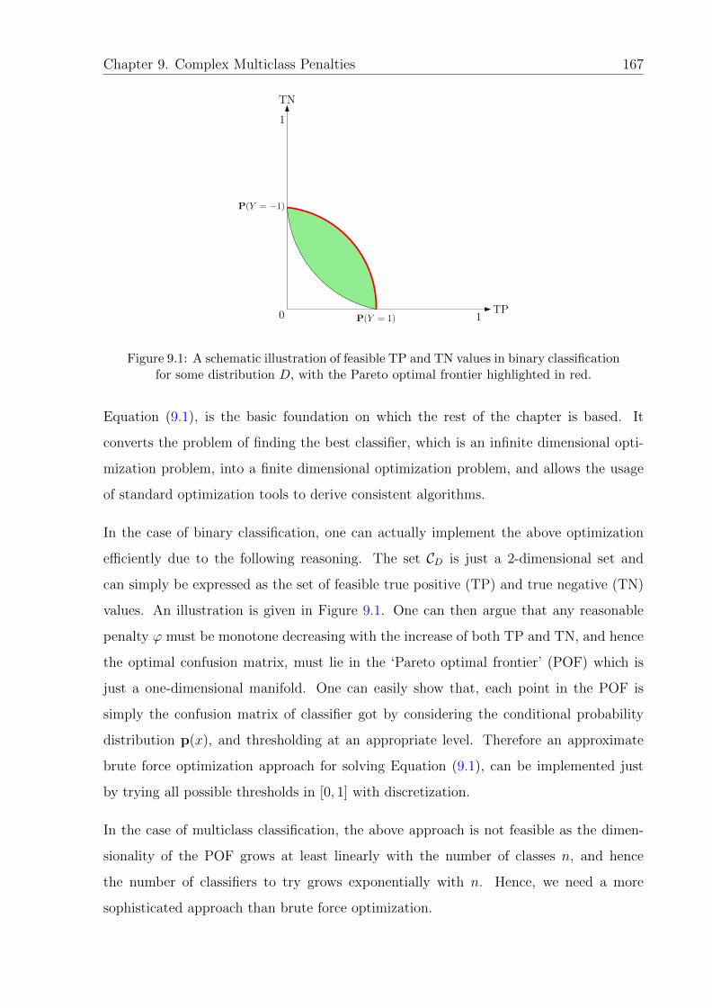
Chapter 9. Complex Multiclass Penalties 167
TP
TN
P(Y = 1)
P(Y = −1)
1
1
0
Figure 9.1: A schematic illustration of feasible TP and TN values in binary classificationfor some distribution D, with the Pareto optimal frontier highlighted in red.
Equation (9.1), is the basic foundation on which the rest of the chapter is based. It
converts the problem of finding the best classifier, which is an infinite dimensional opti-
mization problem, into a finite dimensional optimization problem, and allows the usage
of standard optimization tools to derive consistent algorithms.
In the case of binary classification, one can actually implement the above optimization
efficiently due to the following reasoning. The set CD is just a 2-dimensional set and
can simply be expressed as the set of feasible true positive (TP) and true negative (TN)
values. An illustration is given in Figure 9.1. One can then argue that any reasonable
penalty ϕ must be monotone decreasing with the increase of both TP and TN, and hence
the optimal confusion matrix, must lie in the ‘Pareto optimal frontier’ (POF) which is
just a one-dimensional manifold. One can easily show that, each point in the POF is
simply the confusion matrix of classifier got by considering the conditional probability
distribution p(x), and thresholding at an appropriate level. Therefore an approximate
brute force optimization approach for solving Equation (9.1), can be implemented just
by trying all possible thresholds in [0, 1] with discretization.
In the case of multiclass classification, the above approach is not feasible as the dimen-
sionality of the POF grows at least linearly with the number of classes n, and hence
the number of classifiers to try grows exponentially with n. Hence, we need a more
sophisticated approach than brute force optimization.

Chapter 9. Complex Multiclass Penalties 168
From Proposition 9.1, we immediately have that if ϕ is a convex function over CD, the re-
sulting optimization problem is convex, and hence one can expect efficient algorithms with
a guarantee. Indeed, many complex penalties in practice are convex in CD as indicated
in Table 9.1.
Even assuming the convexity of CD and ϕ, we have a key issue precluding the usage
of standard optimization algorithms like gradient descent – the intractability of the set
CD. Given a confusion matrix C ∈ CD, it is not possible to immediately say if C ∈ CD.
However, thanks to the observation that linear penalties are equivalent to loss matrix
based evaluation metrics, and the observation that for any loss matrix L we have
〈L,CD[h]〉 = EX〈p(X),Lh(X)〉 ,
we immediately have the following.
Proposition 9.2. Let L ∈ Rn×n+ be a loss matrix, with columns `1, . . . , `n. Then any
(deterministic) classifier h∗ : X→[n] satisfying
h∗(x) ∈ argminj∈[n]〈p(x), `j〉
is such that
〈L,CD[h∗]〉 = infh:X→∆n
〈L,CD[h]〉 = infC∈CD〈L,C〉 .
In other words, while checking whether a given confusion matrix C ∈ CD is difficult,
implementing a linear minimization oracle over CD is simple. This observation along
with the observation that the optimization problem given by Equation (9.1) is convex for
a convex penalty ϕ, immediately suggests the usage of the Frank-Wolfe or conditional
gradient [36, 49] algorithm as an apt choice in this situation.
9.4 The BFW Algorithm for Convex Penalties
In this section, we give the details of the Bayes-Frank-Wolfe (BFW) algorithm (see Al-
gorithm 4), which uses finite samples and the Frank-Wolfe algorithm to solve Equation

Chapter 9. Complex Multiclass Penalties 169
(9.1). Further, we give a proof showing the asymptotic consistency of such an algorithm
for convex penalties.
An ideal version of the BFW algorithm for exactly minimizing ϕ(C) over C ∈ CD, having
access to the entire distribution D, would maintain iterates ht : X→∆n,Ct ∈ CD such
that Ct = CD[ht], compute Lt = ∇ϕ(Ct−1), solve the resulting linear minimization
problems minC∈CD〈Lt,C〉 and update Ct and ht. By standard Frank-Wolfe convergence
arguments [49] we have that
ϕ(CD[ht]) = ϕ(Ct) approaches infC∈CD
ϕ(C) = infh:X→∆n
ϕ(CD[ht]) .
However as we only have access to a finite sample S, the above ideal quantities (ht,Ct,Lt)
are replaced by sample dependent quantities (ht, Ct, Lt). The proof technique for show-
ing the consistency of such an algorithm proceeds as though we maintain implicitly the
ideal quantities, and all errors for maintaining the sample dependent quantities are ab-
sorbed into an additive approximation factor for solving the linear minimization problems
minC∈CD〈Lt,C〉. The proof of convergence for the Frank-Wolfe algorithm also holds under
such approximations [49].
The final (randomized) classifier output by the algorithm is a convex combination of the
classifiers learned across all the iterations.
We now show the consistency of the BFW algorithm for convex and smooth penalties.
Theorem 9.3 (ϕ-regret of BFW). Let ϕ : [0, 1]n×n→R+ be convex over CD, and L-
Lipschitz and β-smooth w.r.t. the `1 norm. Let S ∈ (X × [n])M be drawn i.i.d from D.
Let p : X→∆n be the CPE model learned in Algorithm 4 and hBFWS : X→∆n the classifier
returned after κM iterations. Let δ ∈ (0, 1]. Then with probability ≥ 1−δ (over S ∼ DM)
LϕD[hBFWS ]− Lϕ,∗D
≤ 4LEX
[∥∥p(X)− p(X)∥∥
1
]+ 4√
2βn2C
√n2 log(n) log(M) + log(n2/δ)
M+
8β
κM + 2,
where C > 0 is a distribution-independent constant.
The proof of the above theorem proceeds via a sequence of lemmas.
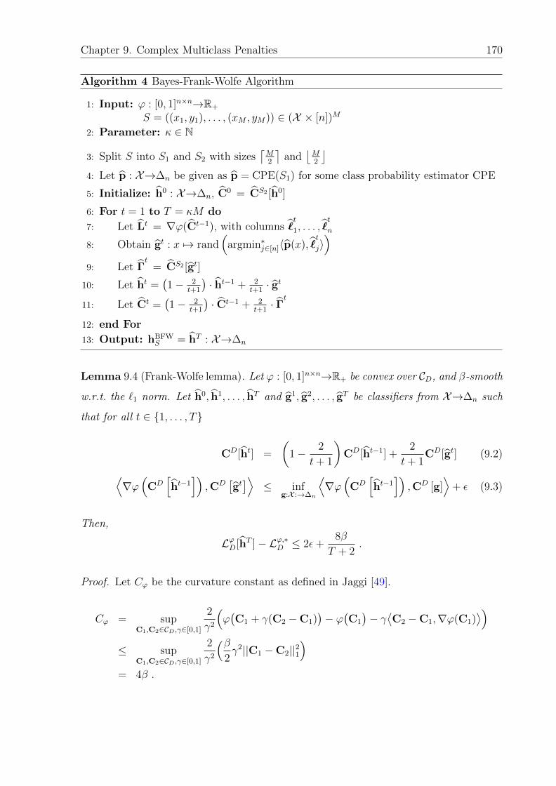
Chapter 9. Complex Multiclass Penalties 170
Algorithm 4 Bayes-Frank-Wolfe Algorithm
1: Input: ϕ : [0, 1]n×n→R+
S = ((x1, y1), . . . , (xM , yM)) ∈ (X × [n])M
2: Parameter: κ ∈ N
3: Split S into S1 and S2 with sizes⌈M2
⌉and
⌊M2
⌋4: Let p : X→∆n be given as p = CPE(S1) for some class probability estimator CPE
5: Initialize: h0 : X→∆n, C0 = CS2 [h0]
6: For t = 1 to T = κM do
7: Let Lt = ∇ϕ(Ct−1), with columns t1, . . . , tn8: Obtain gt : x 7→ rand
(argmin∗j∈[n]〈p(x), tj〉)
9: Let Γt
= CS2 [gt]
10: Let ht =(1− 2
t+1
)· ht−1 + 2
t+1· gt
11: Let Ct =(1− 2
t+1
)· Ct−1 + 2
t+1· Γt
12: end For
13: Output: hBFWS = hT : X→∆n
Lemma 9.4 (Frank-Wolfe lemma). Let ϕ : [0, 1]n×n→R+ be convex over CD, and β-smooth
w.r.t. the `1 norm. Let h0, h1, . . . , hT and g1, g2, . . . , gT be classifiers from X→∆n such
that for all t ∈ 1, . . . , T
CD[ht] =
(1− 2
t+ 1
)CD[ht−1] +
2
t+ 1CD[gt] (9.2)⟨
∇ϕ(CD
[ht−1
]),CD
[gt]⟩≤ inf
g:X :→∆n
⟨∇ϕ
(CD
[ht−1
]),CD [g]
⟩+ ε (9.3)
Then,
LϕD[hT ]− Lϕ,∗D ≤ 2ε+8β
T + 2.
Proof. Let Cϕ be the curvature constant as defined in Jaggi [49].
Cϕ = supC1,C2∈CD,γ∈[0,1]
2
γ2
(ϕ(C1 + γ(C2 −C1)
)− ϕ
(C1
)− γ⟨C2 −C1,∇ϕ(C1)
⟩)≤ sup
C1,C2∈CD,γ∈[0,1]
2
γ2
(β2γ2||C1 −C2||21
)= 4β .
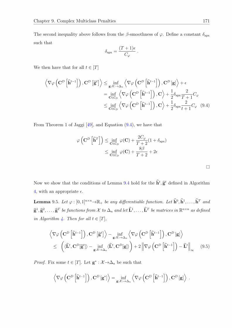
Chapter 9. Complex Multiclass Penalties 171
The second inequality above follows from the β-smoothness of ϕ. Define a constant δapx
such that
δapx =(T + 1)ε
Cϕ.
We then have that for all t ∈ [T ]
⟨∇ϕ
(CD
[ht−1
]),CD
[gt]⟩≤ inf
g:X :→∆n
⟨∇ϕ
(CD
[ht−1
]),CD [g]
⟩+ ε
= infC∈CD
⟨∇ϕ
(CD
[ht−1
]),C⟩
+1
2δapx
2
T + 1Cϕ
≤ infC∈CD
⟨∇ϕ
(CD
[ht−1
]),C⟩
+1
2δapx
2
t+ 1Cϕ (9.4)
From Theorem 1 of Jaggi [49], and Equation (9.4), we have that
ϕ(CD
[hT])≤ inf
C∈CDϕ(C) +
2CϕT + 2
(1 + δapx)
≤ infC∈CD
ϕ(C) +8β
T + 2+ 2ε
Now we show that the conditions of Lemma 9.4 hold for the ht, gt defined in Algorithm
4, with an appropriate ε.
Lemma 9.5. Let ϕ : [0, 1]n×n→R+ be any differentiable function. Let h0, h1, . . . , hT and
g1, g2, . . . , gT be functions from X to ∆n and let L1, . . . , LT be matrices in Rn×n as defined
in Algorithm 4. Then for all t ∈ [T ],
⟨∇ϕ
(CD
[ht−1
]),CD
[gt]⟩− inf
g:X :→∆n
⟨∇ϕ
(CD
[ht−1
]),CD [g]
⟩≤
(〈Lt,CD[gt]〉 − inf
g:X→∆n
〈Lt,CD[g]〉)
+ 2∥∥∥∇ϕ(CD
[ht−1
])− Lt
∥∥∥∞
(9.5)
Proof. Fix some t ∈ [T ]. Let g∗ : X→∆n be such that
⟨∇ϕ
(CD
[ht−1
]),CD [g∗]
⟩= inf
g:X :→∆n
⟨∇ϕ
(CD
[ht−1
]),CD [g]
⟩.

Chapter 9. Complex Multiclass Penalties 172
We then have that
⟨∇ϕ
(CD
[ht−1
]),CD
[gt]⟩− inf
g:X :→∆n
⟨∇ϕ
(CD
[ht−1
]),CD [g]
⟩=
⟨∇ϕ
(CD
[ht−1
]),CD
[gt]⟩−⟨∇ϕ
(CD
[ht−1
]),CD [g∗]
⟩=
⟨∇ϕ
(CD
[ht−1
])− Lt,CD
[gt]⟩−⟨∇ϕ
(CD
[ht−1
])− Lt,CD [g∗]
⟩+(⟨
Lt,CD[gt]⟩−⟨Lt,CD [g∗]
⟩)=
⟨∇ϕ
(CD
[ht−1
])− Lt,CD
[gt]−CD [g∗]
⟩+(⟨
Lt,CD[gt]⟩−⟨Lt,CD [g∗]
⟩)≤
∥∥∥∇ϕ(CD[ht−1
])− Lt
∥∥∥∞· ‖CD
[gt]−CD [g∗] ‖1 +
(〈Lt,CD[gt]〉 − inf
g:X→∆n
〈Lt,CD[g]〉)
≤(〈Lt,CD[gt]〉 − inf
g:X→∆n
〈Lt,CD[g]〉)
+ 2∥∥∥∇ϕ(CD
[ht−1
])− Lt
∥∥∥∞.
The next to last inequality above follows from Holder’s inequality, and the last inequality
follows from the observation that all confusion matrices lie in `1-ball of diameter 2.
It now only remains to bound both terms on the RHS of Equation (9.5).
The first term on the RHS of Equation (9.5) can be bounded using the lemma below and
the observation that the matrices Lt in Algorithm 4 are all such that ||Lt||∞ ≤ L, the
Lipschitz constant of ϕ w.r.t. `1 norm.
Lemma 9.6. For a fixed loss matrix L ∈ Rn×n with columns `1, . . . , `n and class proba-
bility estimation model p : X→∆n, let g : X→∆n be a classifier such that
g(x) = rand(argmin∗j∈[n]〈p(x), `j〉
).
Then
〈L,CD[g]〉 − infg:X→∆n
〈L,CD[g]〉 ≤ 2‖L‖∞ · EX
[∥∥p(X) − p(X)∥∥
1
].
Proof. Let g∗ : X→∆n be such that
g∗(x) = rand(argmin∗j∈[n]〈p(x), `j〉)

Chapter 9. Complex Multiclass Penalties 173
By Proposition 9.2, we have that
g∗ ∈ argming:X→∆n〈L,CD[g]〉 .
We have that
〈L,CD[g]〉 − infg:X→∆n
〈L,CD[g]〉
= 〈L,CD[g]〉 − 〈L,CD[g∗]〉
= EX
[〈p(X),Lg(X)〉
]− EX
[〈p(X),Lg∗(X)〉
]= EX
[〈p(X)− p(X),Lg(X)〉
]+ EX
[〈p(X),Lg(X)〉
]− EX
[〈p(X),Lg∗(X)〉
]≤ EX
[〈p(X)− p(X),Lg(X)〉
]+ EX
[〈p(X),Lg∗(X)〉
]− EX
[〈p(X),Lg∗(X)〉
]= EX
[〈p(X)− p(X),L(g(X)− g∗(X))〉
]≤ 2||L||∞ · EX
[∥∥p(X) − p(X)∥∥
1
].
The last inequality above follows from Holder’s inequality.
The second term on the RHS of Equation (9.5) can be bounded using the two lemmas
below.
Lemma 9.7. Let ϕ : [0, 1]n×n→R+ be β-smooth w.r.t. the `1-norm. Let classifiers
h0, . . . , hT , g1, . . . , gT and matrices L1, . . . , LT be as defined in Algorithm 4. Then for
all t ∈ [T ]
∥∥∥∇ϕ(CD[ht−1
])− Lt
∥∥∥∞≤ βn2 sup
h∈Hp
∥∥CD[h] − CS[h]∥∥∞ .

Chapter 9. Complex Multiclass Penalties 174
Proof. By definition we have Lt = ∇ϕ(CS2
[ht−1
]). Hence,
∥∥∥∇ϕ(CD[ht−1
])− Lt
∥∥∥∞
=∥∥∥∇ϕ(CD
[ht−1
])−∇ϕ
(CS2
[ht−1
])∥∥∥∞
≤ β∥∥CS2
[ht−1
]−CD
[ht−1
] ∥∥1
≤ βn2∥∥CS2
[ht−1
]−CD
[ht−1
] ∥∥∞
≤ βn2 maxi∈[t−1]
∥∥CS2[gi]−CD
[gi] ∥∥∞
≤ βn2 suph∈Hp
∥∥CS2 [h]−CD [h]∥∥∞.
The next to last inequality follows because ht is in the convex hull of g1, . . . , gt. The last
inequality follows because for all t ∈ [T ] there exists a h ∈ Hp such that CD[h] = CD[gt]
and CS2 [h] = CS2 [gt].
Lemma 9.8. Let µ : X→∆n. Let S ∈ (X × [n])M be a sample drawn i.i.d. from DM .
For any δ ∈ (0, 1], w.p. at least 1− δ (over draw of S from DM),
suph∈Hµ
∥∥CD[h] − CS[h]∥∥∞ ≤ C
√n2 log(n) log(M) + log(n2/δ)
M,
where C > 0 is a distribution-independent constant.
Proof. For any a, b ∈ [n] we have,
suph∈Hµ
∣∣∣CSa,b[h]− CD
a,b[h]∣∣∣ = sup
h∈Hµ
∣∣∣∣∣ 1
M
M∑i=1
(1(yi = a, h(xi) = b)− E[1(Y = a, h(X) = b)])
∣∣∣∣∣= sup
h∈Hbµ
∣∣∣∣∣ 1
M
M∑i=1
(1(yi = a, h(xi) = 1)− E[1(Y = a, h(X) = 1)])
∣∣∣∣∣ ,where
Hbµ =
h : X→0, 1 : ∃L ∈ [0, 1]n×n,∀x ∈ X , h(x) = 1
(b = argmin∗j∈[n]〈µ(x), `y〉
).
The set Hbµ can be seen as a binary hypothesis class whose concepts are the intersection
of n halfspaces in Rn (corresponding to µ(x)) through the origin. Hence we have from
Lemma 3.2.3 of Blumer et al. [9] that the VC-dimension of Hbµ is at most 2n2 log(3n).

Chapter 9. Complex Multiclass Penalties 175
From standard uniform convergence arguments we have that the following holds with
probability 1− δ,
suph∈Hµ
∣∣∣CSa,b[h]− CD
a,b[h]∣∣∣ ≤ C
√n2 log(n) log(M) + log(1
δ)
M
where C > 0 is some constant. Applying union bound for all a, b ∈ [n] we have that the
following holds with probability 1− δ
suph∈Hµ
∣∣∣∣∣∣CS[h]−CD[h]∣∣∣∣∣∣∞≤ C
√n2 log(n) log(M) + log(n
2
δ)
M.
The proof of Theorem 9.3 follows from applying Lemmas 9.4, 9.5, 9.6, 9.7, 9.8.
Theorem 9.3 shows that the BFW algorithm, when used with a consistent CPE whose `1
probability estimation error goes to zero, is consistent for convex smooth penalties. How-
ever, many penalties in practice including the GM, HM, QM and the min-max penalties
in Table 9.1 are convex but non-smooth. Theorem 9.3 can be easily extended to such
non-smooth penalties as well due to the observation that, any non-smooth convex func-
tion over a compact domain can be arbitrarily approximated (in the relative interior of its
domain) using a smooth convex function. Hence, applying Algorithm 4 to such a smooth
approximation, with the approximation error going to zero appropriately as the sample
size increases, gives a consistent algorithm for non-smooth convex penalties as well.

Chapter 10
Conclusions and Future Directions
10.1 Summary
In the first part of the thesis, we presented the foundations of a framework to study
consistent surrogate minimizing algorithms for general multiclass learning problems with
arbitrary loss matrix based evaluation metrics. The framework constructed includes sev-
eral important and useful tools that can be used to check whether a surrogate is calibrated
w.r.t. a given loss matrix, to characterize the difficulty of constructing convex calibrated
surrogates for a given loss matrix, and most importantly, to motivate and construct novel
convex calibrated surrogates for specific learning problems.
In the second part of the thesis, we focused particularly on the problem of hierarchical
classification, with the tree distance loss matrix, and gave a template to design convex
calibrated surrogates. In particular, the reduction to the problem of multiclass classi-
fication with an abstain option allows the construction of several SVM-like consistent
algorithms for hierarchical classification, one of which also performs well empirically on
benchmark hierarchical classification datasets.
In the third part of the thesis, we considered complex evaluation metrics more general
than loss matrix based evaluation metrics. We showed that finding the classifier with
the smallest such error is equivalent to a finite dimensional optimization problem with
the linear minimization oracle being the only useful primitive available, and constructed
176

Chapter 9. Conclusions and Future Directions 177
a learning algorithm based on the Frank-Wolfe optimization algorithm that is consistent
for a large family of such complex evaluation metrics.
10.2 Future Directions
While this thesis raises and answers several questions on consistency for multiclass learn-
ing problems that deepen our understanding, it also raises several questions which re-
main unanswered and form interesting directions of future research. We give some of
these questions below, and organize them in accordance with the three main parts of this
thesis.
10.2.1 Consistency and Calibration
• While Theorems 3.7 and 3.9 give necessary conditions and sufficient conditions for
calibration, they are a far cry from the simple characterisation for calibration in
binary classification as in Bartlett et al. [7]. Some extra complexity is necessary
to accommodate the multiclass setting and general predictors rather than just the
sign predictor used in binary classification. But, can one do better than the current
conditions?
• While the convex calibration dimension is an intrinsic notion of difficulty for a
loss matrix, it is not the only one, nor does it fully capture the difficulty of the
entire consistent algorithm. In particular it does not capture the complexity of the
predictor as evidenced by the pairwise disagreement and mean average precision
losses. Is there a better notion for capturing this as well ?
• As has been observed, the upper and lower bounds on the convex calibration di-
mension are not tight in general. Can they be tightened?
• Weakening consistency with noise condition requirements is an excellent way of
trading off computational complexity with generality of assumptions, but charac-
terizing and constructing such algorithms for an arbitrary noise condition and loss
matrix remains hard to do. Can such results be obtained?

Chapter 9. Conclusions and Future Directions 178
10.2.2 Application to Hierarchical Classification
• The existence of a log2(n)-dimensional convex calibrated surrogate for the n-class
abstain(12) loss is an interesting result, but the lower bound on the CC-Dimension
of the abstain(12) loss is actually lower than this (it is in fact just 2 for any n). Can
one show a tighter lower bound on the CC dimension of this loss?
• How do we construct convex calibrated (piecewise linear, SVM-type) surrogates for
the abstain(α) loss when α ∈ [12, 1]?
• The reduction of the hierarchical classification problem to the multiclass classifica-
tion problem with an abstain option is valid only for tree hierarchies. Does there
exist such a result for general graph or at least DAG based hierarchies?
10.2.3 Multiclass Complex Evaluation Metrics
• The optimization viewpoint equating the problem of consistency for multiclass eval-
uation metrics with that of a finite dimensional optimization problem forms a very
useful tool, but the only known useful primitive available to us for the optimization
problem is the linear minimization oracle. Are there any other primitives that can
be used?
• The Bayes-Frank-Wolfe algorithm uses only the linear minimization oracle and is apt
for convex penalties. Harikrishna Narasimhan’s PhD thesis will describe a bisection
algorithm based method which also uses only the linear minimization oracle, and is
apt for penalties that can be expressed as a ratio of linear functions of the confusion
matrix, like the micro F-measure (see also [72]). Are there other interesting complex
penalties used in practice which can be solved with other optimization algorithms
that use only the linear minimization oracle?
• The macro F-measure in multiclass classification is an important multiclass complex
penalty, but unfortunately it is neither convex nor can it be expressed as a ratio of
linear functions. Can one get interesting guarantees for either the Frank-Wolfe or
Chapter 9. Conclusions and Future Directions 179
bisection based algorithm, or give a different algorithm that is consistent for this
performance measure?
10.3 Comments
In conclusion, in this thesis, we have developed a deep understanding and fundamental
results in the theory of supervised multiclass learning. These insights have allowed us to
develop computationally efficient and statistically consistent algorithms for a variety of
multiclass learning problems of practical interest, in many cases significantly outperform-
ing the state-of-the-art algorithms for these problems.

Appendix A
Convexity
Definition A.1 (Convex set). A set C ⊆ Rd is said to be convex if for all x1,x2 ∈ C and
λ ∈ [0, 1] we have that λx1 + (1− λ)x2 ∈ C.
Definition A.2 (Convex function). A function f : C→R is is said to be convex if C is
convex and for all x1,x2 ∈ C and λ ∈ [0, 1] we have that
f(λx1 + (1− λ)x2) ≤ λf(x1) + (1− λ)f(x2) .
Definition A.3 (Strictly convex function). A function f : C→R is is said to be strictly
convex if C is convex and for all x1,x2 ∈ C with x1 6= x2 and λ ∈ (0, 1) we have that
f(λx1 + (1− λ)x2) < λf(x1) + (1− λ)f(x2) .
Proposition A.1 (Minimizers of convex and strictly convex functions). If f : C→R
is a convex function, then all local minimizers are global minimizers. Also the set of
minimizers, argminx∈C f(x), forms a convex set. If f : C→R is a strictly convex function,
then the set of minimizers, argminx∈C f(x), is a singleton.
Definition A.4 (Sub-differentials of a convex function). The sub-differentials of a convex
function f : C→R+, at a point x ∈ C, for some C ⊆ Rd is denoted by ∂f(x) and is given
as
∂f(x) = w ∈ Rd : f(y) ≥ f(x) + 〈w,y − x〉, ∀y ∈ C .
180

Appendix A. Convexity 181
If f is differentiable at x, then ∂f(x) is a singleton containing only ∇f(x).
Definition A.5 (ε-sub-differentials of a convex function). For any ε > 0, the ε-sub-
differentials of a convex function f : C→R+, at a point x ∈ C, for some C ⊆ Rd is
denoted by ∂εf(x) and is given as
∂εf(x) = w ∈ Rd : f(y) ≥ f(x) + 〈w,y − x〉 − ε,∀y ∈ C .
If ε = 0, then ε-sub-differentials are the same as sub-differentials.
Definition A.6 (Convex hull). A convex hull of a set A ⊆ Rd is a subset of Rd, denoted
by conv(A) and is given by
x ∈ Rd : x =
N∑i=1
λixi, for some N ∈ N, λ1, . . . , λN > 0,N∑i=1
λi = 1,x1, . . . ,xN ∈ A.
Definition A.7 (Affine hull). An affine hull of a set A ⊆ Rd is a subset of Rd, denoted
by aff(A) and is given by
x ∈ Rd : x =
N∑i=1
λixi, for some N ∈ N, λ1, . . . , λN ∈ R,N∑i=1
λi = 1,x1, . . . ,xN ∈ A.
Definition A.8 (Minkowski sum). For any two sets A,B ⊆ Rd, the Minkowski sum of Aand B is denoted by A+ B and is given by
A+ B = x ∈ Rd : x = x1 + x2, for some x1 ∈ A,x2 ∈ B .
Proposition A.2 (Properties of ε-sub-differentials of a convex function). Let C ⊆ Rd.
Let f : C→R be a convex function. Then,
• 0 ∈ ∂εf(x0) ⇐⇒ f(x0) ≤ infx∈C
f(x) + ε .
• For any λ > 0, x0 ∈ C,
∂ε(λf(x0)) = λ ∂(ε/λ)f(x0) .

Appendix A. Convexity 182
• Let f = f1 + . . .+ fn for some convex functions fi : C→R. Let x0 ∈ C. Then
∂εf(x0) ⊆ ∂εf1(x0) + . . .+ ∂εfn(x0) ⊆ ∂nεf(x0) .
where the sum of sets is the Minkowski sum.
• ε1 ≤ ε2 =⇒ ∂ε1f(x0) ⊆ ∂ε2f(x0) .

Bibliography
[1] S. Agarwal. Surrogate regret bounds for the area under the ROC curve via strongly
proper losses. In Proceedings of International Conference on Learning Theory
(COLT), 2013.
[2] S. Agarwal. Surrogate regret bounds for bipartite ranking via strongly proper losses.
Journal of Machine Learning Research, 15:1653–1674, 2014.
[3] N. Ailon, M. Charikar, and A. Newman. Aggregating inconsistent information:
Ranking and clustering. Journal of the ACM, 55(5), 2008.
[4] V. Arya, N. Garg, R. Khandekar, A. Myerson, K. Munagala, and V. Pandit. Local
search heuristics for k-median and facility location problems. SIAM Journal of
Computing, 33:544–562, 2004.
[5] R. Babbar, I. Partalas, E. Gaussier, and M.-R. Amin. On flat versus hierarchical
classification in large-scale taxonomies. In Advances in Neural Information Pro-
cessing Systems, 2013.
[6] P. L. Bartlett and M. Wegkamp. Classification with a reject option using a hinge
loss. Journal of Machine Learning Research, 9:1823–1840, 2008.
[7] P. L. Bartlett, M. Jordan, and J. McAuliffe. Convexity, classification and risk
bounds. Journal of the American Statistical Association, 101(473):138–156, 2006.
[8] D. Bertsekas, A. Nedic, and A. Ozdaglar. Convex Analysis and Optimization.
Athena Scientific, 2003.
[9] A. Blumer, A. Ehrenfeucht, D. Haussler, and M. Warmuth. Learnability and the
Vapnik-Chervonenkis dimension. Journal of the ACM, 36:929–965, 1989.
183

Bibliography 184
[10] S. Boyd and L. Vandenberghe. Convex Optimization. Cambridge university press,
2004.
[11] D. Buffoni, C. Calauzenes, P. Gallinari, and N. Usunier. Learning scoring func-
tions with order-preserving losses and standardized supervision. In Proceedings of
International Conference on Machine Learning, 2011.
[12] A. Buja, W. Stuetzle, and Y. Shen. Loss functions for binary class probability esti-
mation and classification: Structure and applications. Technical report, University
of Pennsylvania, November 2005.
[13] C. Burges, T. Shaked, E. Renshaw, A. Lazier, M. Deeds, N. Hamilton, and G.
Hullender. Learning to rank using gradient descent. In Proceedings of International
Conference on Machine Learning, 2005.
[14] C. Burges, Q. V. Le, and R. R. Learning to rank with nonsmooth cost functions.
In Advances in Neural Information Processing Systems, 1997.
[15] F. Burkhardt, A. Paeschke, M. Rolfes, W. Sendlmeier, and B. Weiss. A database of
german emotional speech. In Proceedings of the 9th European conference on speech
communication and technology, 2005.
[16] L. Cai and T. Hofmann. Hierarchical document categorization with support vector
machines. In International Conference on Information and Knowledge Management
(CIKM), 2004.
[17] C. Calauzenes, N. Usunier, and P. Gallinari. On the (non-)existence of convex, cal-
ibrated surrogate losses for ranking. In Advances in Neural Information Processing
Systems, 2012.
[18] N. Cesa-Bianchi, C. Gentile, and L. Zaniboni. Hierarchical classification: combining
Bayes with SVM. In Proceedings of International Conference on Machine Learning,
2006.
[19] N. Cesa-Bianchi, C. Gentile, and L. Zaniboni. Incremental algorithms for hierar-
chical classification. Journal of Machine Learning Research, 7:31–54, 2006.

Bibliography 185
[20] D.-R. Chen and T. Sun. Consistency of multiclass empirical risk minimization
methods based on convex loss. Journal of Machine Learning Research, 7:2435–
2447, 2006.
[21] C. Chow. On optimum recognition error and reject tradeoff. IEEE Transactions
on Information Theory, 16:41–46, 1970.
[22] S. Clemencon and N. Vayatis. Ranking the best instances. Journal of Machine
Learning Research, 8:2671–2699, 2007.
[23] S. Clemencon, G. Lugosi, and N. Vayatis. Ranking and empirical minimization of
U-statistics. Annals of Statistics, 36:844–874, 2008.
[24] W. W. Cohen, R. E. Schapire, and Y. Singer. Learning to order things. In Advances
in Neural Information Processing Systems, 1997.
[25] D. Cossock and T. Zhang. Statistical analysis of Bayes optimal subset ranking.
IEEE Transactions on Information Theory, 54(11):5140–5154, 2008.
[26] T. Cover and P. Hart. Nearest neighbor pattern classification. IEEE Transactions
on Information Theory, 13(1):21–27, 1967.
[27] K. Crammer and Y. Singer. On the algorithmic implementation of multiclass kernel-
based vector machines. Journal of Machine Learning Research, 2:265–292, 2001.
[28] O. Dekel, C. D. Manning, and Y. Singer. Log-linear models for label ranking. In
Advances in Neural Information Processing Systems, 2003.
[29] O. Dekel, J. Keshet, and Y. Singer. Large margin hierarchical classification. In
Proceedings of International Conference on Machine Learning, 2004.
[30] K. Dembczynski, W. Waegeman, W. Cheng, and E. Hullermeier. An exact algo-
rithm for F-measure maximization. In Advances in Neural Information Processing
Systems 25, 2011.

Bibliography 186
[31] K. Dembczynski, A. Jachnik, W. Kotlowski, W. Waegeman, and E. Hullermeier.
Optimizing the f-measure in multi-label classification: Plug-in rule approach ver-
sus structured loss minimization. In Proceedings of International Conference on
Machine Learning, 2013.
[32] I. Dimitrovski, D. Kocev, L. Suzana, and S. Dzeroski. Hierchical annotation of
medical images. Pattern Recognition, 2011.
[33] J. Duchi, S. Shalev-Shwartz, Y. Singer, and T. Chandra. Efficient projections
onto the l1 -ball for learning in high dimensions. In Proceedings of International
Conference on Machine Learning, 2008.
[34] J. Duchi, L. Mackey, and M. Jordan. On the consistency of ranking algorithms. In
Proceedings of International Conference on Machine Learning, 2010.
[35] R. Fan, K. Chang, C. Hsieh, X. Wang, and C. Lin. Liblinear: A library for large
linear classification. Journal of Machine Learning Research, 9:1871–1874, 2008.
[36] M. Frank and P. Wolfe. An algorithm for quadratic programming. Naval Research
Logistics Quarterly, 3(1-2):95–110, 1956.
[37] Y. Freund, R. Iyer, R. E. Schapire, , and Y. Singer. An efficient boosting algorithm
for combining preferences. Journal of Machine Learning Research, 4:933–969, 2003.
[38] G. Fumera and F. Roli. Suppport vector machines with embedded reject option.
Pattern Recognition with Support Vector Machines, pages 68–82, 2002.
[39] G. Fumera and F. Roli. Analysis of error-reject trade-off in linearly combined
multiple classifiers. Pattern Recognition, 37:1245–1265, 2004.
[40] G. Fumera, F. Roli, and G. Giacinto. Reject option with multiple thresholds.
Pattern Recognition, 33:2099–2101, 2000.
[41] G. Fumera, I. Pillai, and F. Roli. Classification with reject option in text categorisa-
tion systems. In IEEE International Conference on Image Analysis and Processing,
pages 582–587, 2003.

Bibliography 187
[42] J. Gallier. Notes on convex sets, polytopes, polyhedra, combinatorial topology,
Voronoi diagrams and Delaunay triangulations. Technical report, Department of
Computer and Information Science, University of Pennsylvania, 2009.
[43] W. Gao and Z.-H. Zhou. On the consistency of multi-label learning. In Proceedings
of International Conference on Learning Theory, 2011.
[44] M. Golfarelli, D. Maio, and D. Maltoni. On the error-reject trade-off in biometric
verification systems. IEEE Transactions on Pattern Analysis and Machine Intelli-
gence, 19:786–796, 1997.
[45] S. Gopal and Y. Yang. Recursive regularization for large-scale classification with
hierarchical and graphical dependencies. In International Conference on Knowledge
Discovery and Data Mining (KDD), 2013.
[46] S. Gopal, B. Bai, Y. Yang, and A. Niculescu-Mizil. Bayesian models for large-scale
hierarchical classification. In Advances in Neural Information Processing Systems
25, 2012.
[47] Y. Grandvalet, A. Rakotomamonjy, J. Keshet, and S. Canu. Support vector ma-
chines with a reject option. In Advances in Neural Information Processing Systems,
2008.
[48] R. Herbrich, T. Graepel, and K. Obermayer. Large margin rank boundaries for or-
dinal regression. In Smola, Bartlett, Schoelkopf, and Schurmaans, editors, Advances
in Large Margin Classifiers. MIT Press, Cambridge, MA, 2000.
[49] M. Jaggi. Revisiting Frank-Wolfe: Projection-free sparse convex optimization. In
Proceedings of International Conference on Machine Learning, 2013.
[50] K. Jain, M. Mahdian, and A. Saberi. A new greedy approach for facility location
problems. In Symposium on Theory of Computing (STOC), 2002.
[51] K. Jarvelin and J. Kekalainen. IR evaluation methods for retrieving highly relevant
documents. In International ACM SIGIR Conference on Research and Development
in Information Retrieval, 2000.

Bibliography 188
[52] W. Jiang. Process consistency for AdaBoost. Annals of Statistics, 32(1):13–29,
2004.
[53] T. Joachims. A support vector method for multivariate performance measures. In
Proceedings of International Conference on Machine Learning, 2005.
[54] T. Joachims. Optimizing search engines using clickthrough data. In ACM Confer-
ence on Knowledge Discovery and Data Mining (KDD), 2002.
[55] T. Joachims. Making large-scale svm learning practical. In B. Scholkopf, C. Burges,
and A. Smola, editors, Advances in Kernel Methods - Support Vector Learning.
MIT-Press, 1999.
[56] K. Kennedy, B. Namee, and S. Delany. Learning without default: A study of
one-class classification and the low-default portfolio problem. In ICAICS, 2009.
[57] C. Kenyon-Mathieu and W. Schudy. How to rank with few errors. In Symposium
on Theory of Computing (STOC), 2007.
[58] J.-D. Kim, Y. Wang, and Y. Yasunori. The genia event extraction shared task,
2013 edition - overview. Association of Computational Linguistics, 2013.
[59] S. Koco and C. Capponi. On multi-class classification through the minimization of
the confusion matrix norm. In ACML, 2013.
[60] W. Kotlowski, K. Dembczynski, and E. Huellermeier. Bipartite ranking through
minimization of univariate loss. In Proceedings of International Conference on Ma-
chine Learning, 2011.
[61] O. Koyejo, N. Natarajan, P. Ravikumar, and I. Dhillon. Consistent binary classi-
fication with generalized performance metrics. In Advances in Neural Information
Processing Systems, 2014.
[62] N. Lambert and Y. Shoham. Eliciting truthful answers to multiple-choice questions.
In ACM Conference on Electronic Commerce, 2009.

Bibliography 189
[63] S. Lawrence, I. Burns, A. Back, A.-C. Tsoi, and C. Giles. Neural network classifica-
tion and prior class probabilities. In Neural Networks: Tricks of the Trade, LNCS,
pages 1524:299–313. Springer, 1998.
[64] Y. Lee, Y. Lin, and G. Wahba. Multicategory support vector machines: Theory
and application to the classification of microarray data. Journal of the American
Statistical Association, 99(465):67–81, 2004.
[65] D. Lewis. Evaluating text categorization. In Proceedings of the Workshop on Speech
and Natural Language, HLT ’91, 1991.
[66] G. Lugosi and N. Vayatis. On the Bayes-risk consistency of regularized boosting
methods. Annals of Statistics, 32(1):30–55, 2004.
[67] P. Machart and L. Ralaivola. Confusion matrix stability bounds for multiclass
classification. Technical report, Aix-Marseille University, 2012.
[68] C. D. Manning, P. Raghavan, and H. Schtze. Introduction to Information Retrieval.
Cambridge University Press, 2008.
[69] A. Menon, H. Narasimhan, S. Agarwal, and S. Chawla. On the statistical consis-
tency of algorithms for binary classification under class imbalance. In Proceedings
of International Conference on Machine Learning, 2013.
[70] D. Musicant, V. Kumar, and A. Ozgur. Optimizing F-measure with support vector
machines. In FLAIRS, 2003.
[71] H. Narasimhan, R. Vaish, and S. Agarwal. On the statistical consistency of plug-
in classifiers for non-decomposable performance measures. In Advances in Neural
Information Processing Systems, 2014.
[72] H. Narasimhan*, H. G. Ramaswamy*, A. Saha, and S. Agarwal. Consistent multi-
class algorithms for complex performance measures. In Proceedings of International
Conference on Machine Learning, 2015.
[73] D. O’Brien, M. Gupta, and R. Gray. Cost-sensitive multi-class classification from
probability estimates. In Proceedings of International Conference on Machine
Learning, 2008.

Bibliography 190
[74] S. Parambath, N. Usunier, and Y. Grandvalet. Optimizing F-measures by cost-
sensitive classification. In Advances in Neural Information Processing Systems,
2014.
[75] J. Petterson and T. Caetano. Reverse multi-label learning. In Advances in Neural
Information Processing Systems, 2010.
[76] J. Petterson and T. Caetano. Submodular multi-label learning. In Advances in
Neural Information Processing Systems, 2011.
[77] B. A. Pires, C. Szepesvari, and M. Ghavamzadeh. Cost-sensitive multiclass classifi-
cation risk bounds. In Proceedings of International Conference on Machine Learn-
ing, 2013.
[78] L. Ralaivola. Confusion-based online learning and a passive-aggressive scheme. In
Advances in Neural Information Processing Systems, 2012.
[79] H. G. Ramaswamy and S. Agarwal. Classification calibration dimension for general
multiclass losses. In Advances in Neural Information Processing Systems, 2012.
[80] H. G. Ramaswamy, S. Agarwal, and A. Tewari. Convex calibrated surrogates for
low-rank loss matrices with applications to subset ranking losses. In Advances in
Neural Information Processing Systems, 2013.
[81] H. G. Ramaswamy, B. S. Babu, S. Agarwal, and R. C. Williamson. On the con-
sistency of output code based learning algorithms for multiclass learning problems.
In Proceedings of International Conference on Learning Theory, 2014.
[82] H. G. Ramaswamy, S. Agarwal, and A. Tewari. Convex calibrated surrogates for
hierarchical classification. In Proceedings of International Conference on Machine
Learning, 2015.
[83] P. Ravikumar, A. Tewari, and E. Yang. On NDCG consistency of listwise ranking
methods. In International Conference on Artificial Intelligence and Statistics, 2011.
[84] M. D. Reid and R. C. Williamson. Composite binary losses. Journal of Machine
Learning Research, 11:2387–2422, 2010.

Bibliography 191
[85] M. D. Reid and R. C. Williamson. Information, divergence and risk for binary
experiments. Journal of Machine Learning Research, 11:731–817, 2011.
[86] R. Rifkin and A. Klautau. In defense of one-vs-all classification. Journal of Machine
Learning Research, 5:101–141, 2004.
[87] J. Rousu, C. Saunders, S. Szedmak, and J. Shawe-Taylor. Kernel-based learning of
hierarchical multilabel classification models. Journal of Machine Learning Research,
7:1601–1626, 2006.
[88] L. Savage. Elicitation of personal probabilities and expectations. Journal of the
American Statistical Association, 66(336):783–801, 1971.
[89] M. Schervish. A general method for comparing probability assessors. Annals of
Statistics, 17(4):1856–1879, 1989.
[90] C. Scott. Calibrated asymmetric surrogate losses. Electronic Journal of Statistics,
6:958–992, 2012.
[91] E. Shuford, A. Albert, and H. Massengill. Admissible probability measurement
procedures. Psychometrika, 31(2):125–145, 1966.
[92] C. N. Silla Jr. and A. A. Freitas. A survey of hierarchical classification across
different application domains. Data Mining and Knowledge Discovery, 2011.
[93] P. Simeone, C. Marrocco, and F. Tortorella. Design of reject rules for ECOC
classification systems. Pattern Recognition, 45:863–875, 2012.
[94] I. Steinwart. Consistency of support vector machines and other regularized kernel
classifiers. IEEE Transactions on Information Theory, 51(1):128–142, 2005.
[95] I. Steinwart. How to compare different loss functions and their risks. Constructive
Approximation, 26:225–287, 2007.
[96] C. J. Stone. Consistent nonparametric regression. Annals of Statistics, 5(4):595–
620, 1977.
[97] A. Sun and E.-P. Lim. Hierarchical text classification and evaluation. In Proceedings
of International Conference on Data Mining, 2001.
Bibliography 192
[98] Y. Sun, M. Kamel, and Y. Wang. Boosting for learning multiple classes with
imbalanced class distribution. In Proceedings of International Conference on Data
Mining, 2006.
[99] A. Tamir. An O(pn2) algorithm for the p-median and related problems on tree
graphs. Operations Research letters, 19:59–64, 1996.
[100] A. Tewari and P. L. Bartlett. On the consistency of multiclass classification meth-
ods. Journal of Machine Learning Research, 8:1007–1025, 2007.
[101] I. Tsochantiridis, T. Joachims, T. Hoffman, and Y. Altun. Large margin methods
for structured and interdependent output variables. Journal of Machine Learning
Research, 6:1453–1484, 2005.
[102] A. B. Tsybakov. Optimal aggregation of classifiers in statistical learning. Annals
of Statistics, 32(1):135–166, 2004.
[103] E. Vernet, R. C. Williamson, and M. D. Reid. Composite multiclass losses. In
Advances in Neural Information Processing Systems, 2011.
[104] P. Vincent. An Introduction to Signal Detection and Estimation. Springer-Verlag
New York, Inc., 1994.
[105] H. Wang, X. Shen, and W. Pan. Large margin hierarchical classification with
mutually exclusive class membership. Journal of Machine Learning Research, 12:
2721–2748, 2011.
[106] K. Wang, S. Zhou, and S. C. Liew. Building hierarchical classifiers using class
proximity. In International Conference on Very Large Data Bases, 1999.
[107] P.-W. Wang and C.-J. Lin. Iteration complexity of feasible descent methods for
convex optimization. Journal of Machine Learning Research, 15:1523–1548, 2014.
[108] S. Wang and X. Yao. Multiclass imbalance problems: Analysis and potential solu-
tions. IEEE Transactions on Systems, Man, and Cybernetics, Part B: Cybernetics,
42(4):1119–1130, 2012.
Bibliography 193
[109] J. Weston and C. Watkins. Support vector machines for multi-class pattern recog-
nition. In 7th European Symposium On Artificial Neural Networks, 1999.
[110] Q. Wu, C. Jia, and W. Chen. A novel classification-rejection sphere SVMs for
multi-class classification problems. In IEEE International Conference on Natural
Computation, 2007.
[111] F. Xia, T.-Y. Liu, J. Wang, W. Zhang, and H. Li. Listwise approach to learning
to rank: Theory and algorithm. In Proceedings of International Conference on
Machine Learning, 2008.
[112] Z. Xiao, E. Dellandrea, W. Dou, and L. Chen. Hierarchical classification of emo-
tional speech. IEEE Transactions on Multimedia, 2007.
[113] N. Ye, K. Chai, W. Lee, and H. Chieu. Optimizing F-measures: A tale of two
approaches. In Proceedings of International Conference on Machine Learning, 2012.
[114] M. Yuan and M. Wegkamp. Classification methods with reject option based on
convex risk minimization. Journal of Machine Learning Research, 11:111–130, 2010.
[115] T. Zhang. Statistical behavior and consistency of classification methods based on
convex risk minimization. Annals of Statistics, 32(1):56–134, 2004.
[116] T. Zhang. Statistical analysis of some multi-category large margin classification
methods. Journal of Machine Learning Research, 5:1225–1251, 2004.
[117] C. Zou, E. Zheng, H. Xu, and L. Chen. Cost-sensitive multi-class SVM with reject
option: A method for steam turbine generator fault diagnosis. International Journal
of Computer Theory and Engineering, 2011.