Consistent Algorithms for Clustering Time Serieskhaleghi/Publications_files/khaleghi16a.pdf ·...

Journal of Machine Learning Research 17 (2016) 1-32 Submitted 7/13; Revised 12/14; Published 3/16

Consistent Algorithms for Clustering Time Series

Azadeh Khaleghi [email protected] of Mathematics & StatisticsLancaster University, Lancaster, LA1 4YF, UK

Daniil Ryabko [email protected] Lille40, avenue de Halley59650 Villeneuve d’Ascq, France

Jeremie Mary [email protected]

Philippe Preux [email protected]

Universite de Lille/CRIStAL (UMR CNRS)

40, avenue de Halley

59650 Villeneuve d’Ascq, France

Editor: Gabor Lugosi

Abstract

The problem of clustering is considered for the case where every point is a time series.The time series are either given in one batch (offline setting), or they are allowed to growwith time and new time series can be added along the way (online setting). We proposea natural notion of consistency for this problem, and show that there are simple, com-putationally efficient algorithms that are asymptotically consistent under extremely weakassumptions on the distributions that generate the data. The notion of consistency is asfollows. A clustering algorithm is called consistent if it places two time series into the samecluster if and only if the distribution that generates them is the same. In the consideredframework the time series are allowed to be highly dependent, and the dependence canhave arbitrary form. If the number of clusters is known, the only assumption we makeis that the (marginal) distribution of each time series is stationary ergodic. No paramet-ric, memory or mixing assumptions are made. When the number of clusters is unknown,stronger assumptions are provably necessary, but it is still possible to devise nonparametricalgorithms that are consistent under very general conditions. The theoretical findings ofthis work are illustrated with experiments on both synthetic and real data.

Keywords: clustering, time series, ergodicity, unsupervised learning

1. Introduction

Clustering is a widely studied problem in machine learning, and is key to many applicationsacross different fields of science. The goal is to partition a given data set into a set of non-overlapping clusters in some natural way, thus hopefully revealing an underlying structurein the data. In particular, this problem for time series data is motivated by many researchproblems from a variety of disciplines, such as marketing and finance, biological and medicalresearch, video/audio analysis, etc., with the common feature that the data are abundantwhile little is known about the nature of the processes that generate them.

c©2016 Azadeh Khaleghi, Daniil Ryabko, Jeremie Mary and Philippe Preux.

Khaleghi, Ryabko, Mary and Preux

The intuitively appealing problem of clustering is notoriously difficult to formalise. Anintrinsic part of the problem is a similarity measure: the points in each cluster are supposedto be close to each other in some sense. While it is clear that the problem of finding theappropriate similarity measure is inseparable from the problem of achieving the clusteringobjectives, in the available formulations of the problem it is usually assumed that thesimilarity measure is given: it is either some fixed metric, or just a matrix of similaritiesbetween the points. Even with this simplification, it is still unclear how to define goodclustering. Thus, Kleinberg (2002) presents a set of fairly natural properties that a goodclustering function should have, and further demonstrate that there is no clustering functionthat satisfies these properties. A common approach is therefore to fix not only the similaritymeasure, but also some specific objective function — typically, along with the number ofclusters — and to construct algorithms that maximise this objective. However, even thisapproach has some fundamental difficulties, albeit of a different, this time computational,nature: already in the case where the number of clusters is known, and the distance betweenthe points is set to be the Euclidean distance, optimising some fairly natural objectives (suchas k-means) turns out to be NP hard (Mahajan et al., 2009).

In this paper we consider a subset of the clustering problem, namely, clustering timeseries. That is, we consider the case where each data point is a sample drawn from some(unknown) time-series distribution. At first glance this does not appear to be a simplifica-tion (indeed, any data point can be considered as a time series of length 1). However, notethat time series present a different dimension of asymptotic: with respect to their length,rather than with respect to the total number of points to be clustered. “Learning” alongthis dimension turns out to be easy to define, and allows for the construction of consistentalgorithms under most general assumptions. Specifically, the assumption that each timeseries is generated by a stationary ergodic distribution is already sufficient to estimate anyfinite-dimensional characteristic of the distribution with arbitrary precision, provided theseries is long enough. Thus, in contrast to the general clustering setup, in the time-seriescase it is possible to “learn” the distribution that generates each given data point. Noassumptions on the dependence between time series are necessary for this. The assumptionthat a given time series is stationary ergodic is one of the most general assumptions usedin statistics; in particular, it allows for arbitrary long-range serial dependence, and sub-sumes most of the nonparametric as well as modelling assumptions used in the literatureon clustering time series, such as i.i.d., (hidden) Markov, or mixing time series.

This allows us to define the following clustering objective: group a pair of time seriesinto the same cluster if and only if the distribution that generates them is the same.

Note that this intuitive objective is impossible to achieve outside the time-series frame-work. Even in the simplest case where the underlying distributions are Gaussian and thenumber of clusters is known, there is always a nontrivial likelihood for each point to be gen-erated by any of the distributions. Thus, the best one can do is to estimate the parametersof the distributions, rather than to actually cluster the data points. The situation becomeshopeless in the nonparametric setting. In contrast, the fully nonparametric case is tractablefor time-series data, both in offline and online scenarios, as explained in the next section.

2


1.1 Problem Setup

We consider two variants of the clustering problem in this setting: offline (batch) and online,defined as follows.

In the offline (batch) setting a finite number N of sequences x1 = (X11 , . . . , X

1n1

),. . . ,xN = (XN

1 , . . . , XNnN

) is given. Each sequence is generated by one of κ different un-known time-series distributions. The target clustering is the partitioning of x1, . . . ,xN intoκ clusters, putting together those and only those sequences that were generated by the sametime-series distribution. We call a batch clustering algorithm asymptotically consistent if,with probability 1, it stabilises on the target clustering in the limit as the lengths n1, . . . , nNof each of the N samples tend to infinity. The number κ of clusters may be either knownor unknown. Note that the asymptotic is not with respect to the number of sequences, butwith respect to the individual sequence lengths.

In the online setting we have a growing body of sequences of data. The number of se-quences as well as the sequences themselves grow with time. The manner of this evolutioncan be arbitrary; we only require that the length of each individual sequence tend to infin-ity. Similarly to the batch setting, the joint distribution generating the data is unknown.At time step 1 initial segments of some of the first sequences are available to the learner.At each subsequent time step, new data are revealed, either as an extension of a previ-ously observed sequence, or as a new sequence. Thus, at each time step t a total of N(t)sequences x1, . . . ,xN(t) are to be clustered, where each sequence xi is of length ni(t) ∈ Nfor i = 1..N(t). The total number of observed sequences N(t) as well as the individualsequence lengths ni(t) grow with time. In the online setting, a clustering algorithm is calledasymptotically consistent, if almost surely for each fixed batch of sequences x1, . . . ,xN ,the clustering restricted to this sequences coincides with the target clustering from sometime on.

At first glance it may seem that one can use the offline algorithm in the online settingby simply applying it to the entire data observed at every time step. However, this naiveapproach does not result in a consistent algorithm. The main challenge in the online settingcan be identified with what we regard as “bad” sequences: sequences for which sufficientinformation has not yet been collected, and thus cannot be distinguished based on the pro-cess distributions that generate them. In this setting, using a batch algorithm at every timestep results in not only mis-clustering such “bad” sequences, but also in clustering incor-rectly those for which sufficient data are already available. That is, such “bad” sequencescan render the entire batch clustering useless, leading the algorithm to incorrectly clustereven the “good” sequences. Since new sequences may arrive in an uncontrollable (evendata-dependent, adversarial) fashion, any batch algorithm will fail in this scenario.

1.2 Results

The first result of this work is a formal definition of the problem of time-series clusteringwhich is rather intuitive, and at the same time allows for the construction of efficientalgorithms that are provably consistent under the most general assumptions. The secondresult is the construction of such algorithms.

More specifically, we propose clustering algorithms that, as we further show, are stronglyasymptotically consistent, provided that the number κ of clusters is known, and the process

3


distribution generating each sequence is stationary ergodic. No restrictions are placed onthe dependence between the sequences: this dependence may be arbitrary (and can bethought of as adversarial). This consistency result is established in each of the two settings(offline and online) introduced above.

As follows from the theoretical impossibility results of Ryabko (2010c) that are discussedfurther in Section 1.4, under the only assumption that the distributions generating thesequences are stationary ergodic, it is impossible to find the correct number of clustersκ, that is, the total number of different time-series distributions that generate the data.Moreover, non-asymptotic results (finite-time bounds on the probability of error) are alsoprovably impossible to obtain in this setting, since this is already the case for the problemof estimating the probability of any finite-time event (Shields, 1996).

Finding the number κ of clusters, as well as obtaining non-asymptotic performanceguarantees, is possible under additional conditions on the distributions. In particular, weshow that if κ is unknown, it is possible to construct consistent algorithms provided thatthe distributions are mixing and bounds on the mixing rates are available.

However, the main focus of this paper remains on the general framework where noadditional assumptions on the unknown process distributions are made (other than thatthey are stationary ergodic). As such, the main theoretical and experimental results concernthe case of known κ.

Finally, we show that our methods can be implemented efficiently: they are at mostquadratic in each of their arguments, and are linear (up to log terms) in some formulations.To test the empirical performance of our algorithms we evaluated them on both syntheticand real data. To reflect the generality of the suggested framework in the experimentalsetup, we had our synthetic data generated by stationary ergodic process distributionsthat do not belong to any “simpler” class of distributions, and in particular cannot bemodelled as hidden Markov processes with countable sets of states. In the batch setting,the error rates of both methods go to zero with sequence length. In the online settingwith new samples arriving at every time step, the error rate of the offline algorithm remainsconsistently high, whereas that of the online algorithm converges to zero. This demonstratesthat, unlike the offline algorithm, the online algorithm is robust to “bad” sequences. Todemonstrate the applicability of our work to real-world scenarios, we chose the problem ofclustering motion-capture sequences of human locomotion. This application area has alsobeen studied in the works (Li and Prakash, 2011) and (Jebara et al., 2007) that (to thebest of our knowledge) constitute the state-of-the-art performance1 on the data sets theyconsider, and against which we compare the performance of our methods. We obtainedconsistently better performance on the data sets involving motion that can be consideredergodic (walking, running), and competitive performance on those involving non-ergodicmotions (single jumps).

1. After this paper had been accepted for publication and entered the production stage, the work (Tschan-nen and Bolcskei, 2015) appeared, which uses the data set of Li and Prakash (2011) and reports a betterperformance on it as compared to both our algorithm and that of Li and Prakash (2011).

4


1.3 Methodology and Algorithms

A crucial point of any clustering method is the similarity measure. Since the objective inour formulation is to cluster time series based on the distributions that generate them, thesimilarity measure must reflect the difference between the underlying distributions. As weaim to make as few assumptions as possible on the distributions that generate the data, andsince we make no assumptions on the nature of differences between the distributions, thedistance should take into account all possible differences between time-series distributions.Moreover, it should be possible to construct estimates of this distance that are consistentfor arbitrary stationary ergodic distributions.

It turns out that a suitable distance for this purpose is the so-called distributional dis-tance. The distributional distance d(ρ1, ρ2) between a pair of process distributions ρ1, ρ2

is defined (Gray, 1988) as∑

j∈Nwj |ρ1(Bj)− ρ2(Bj)| where, wj are positive summable realweights, e.g. wj = 1/j(j + 1), and Bj range over a countable field that generates the σ-algebra of the underlying probability space. For example, consider finite-alphabet processeswith the binary alphabet X = {0, 1}. In this case Bj , j ∈ N would range over the setX ∗ = ∪m∈NXm; that is, over all tuples 0, 1, 00, 01, 10, 11, 000, 001, . . . ; therefore, the dis-tributional distance in this case is the weighted sum of the differences of the probabilityvalues (calculated with respect to ρ1 and ρ2) of all possible tuples. In this case, the dis-tributional distance metrises the topology of weak convergence. In this work we considerreal-valued processes so that the sets Bj range over a suitable sequence of intervals, all pairsof such intervals, triples, and so on (see the formal definitions in Section 2). Although thisdistance involves infinite summations, we show that its empirical approximations can beeasily calculated. Asymptotically consistent estimates of this distance can be obtained byreplacing unknown probabilities with the corresponding frequencies (Ryabko and Ryabko,2010); these estimators have proved useful in various statistical problems concerning ergodicprocesses (Ryabko and Ryabko, 2010; Ryabko, 2012; Khaleghi and Ryabko, 2012).

Armed with an estimator of the distributional distance, it is relatively easy to constructa consistent clustering algorithm for the batch setting. In particular, we show that thefollowing algorithm is asymptotically consistent. First, a set of κ cluster centres are chosenby κ farthest point initialisation (using an empirical estimate of the distributional distance).This means that the first sequence is assigned as the first cluster centre. Iterating over 2..κ,at every iteration a sequence is sought which has the largest minimum distance from thealready chosen cluster centres. Next, the remaining sequences are assigned to the closestclusters.

The online algorithm is based on a weighted combination of several clusterings, eachobtained by running the offline procedure on different portions of data. The partitions arecombined with weights that depend on the batch size and on an appropriate performancemeasure for each individual partition. The performance measure of each clustering is theminimum inter-cluster distance.

1.4 Related Work

Some probabilistic formulations of the time-series clustering problem can be consideredrelated to ours. Perhaps the closest is in terms of mixture models (Bach and Jordan,2004; Biernacki et al., 2000; Kumar et al., 2002; Smyth, 1997; Zhong and Ghosh, 2003):

5


it is assumed that the data are generated by a mixture of κ different distributions thathave a particular known form (such as Gaussian, Hidden Markov models, or graphicalmodels). Thus, each of the N samples is independently generated according to one ofthese κ distributions (with some fixed probability). Since the model of the data is specifiedquite well, one can use likelihood-based distances (and then, for example, the k-meansalgorithm), or Bayesian inference, to cluster the data. Another typical objective is toestimate the parameters of the distributions in the mixture (e.g., Gaussians), rather thanactually clustering the data points. Clearly, the main difference between this setting andours is in that we do not assume any known model for the data; we do not even requireindependence between the samples.

Taking a different perspective, the problem of clustering in our formulations generalisestwo classical problems in mathematical statistics, namely, homogeneity testing (or the two-sample problem) and process classification (or the three-sample problem). In the two-sampleproblem, given two sequences x1 = (X1

1 , . . . , X1n1

) and x2 = (X21 , . . . , X

2n2

) it is required totest whether they are generated by the same or by different process distributions. Thiscorresponds to the special case of clustering only N = 2 data points where the number κ ofclusters is unknown: it can be either 1 or 2. In the three-sample problem, three sequencesx1,x2,x3 are given, and it is known that x1 and x2 are generated by different distributions,while x3 is generated either by the same distribution as x1 or by the same distribution asx2. It is required to find which one is the case. This can be seen as clustering N = 3 datapoints, with the number of clusters known: κ = 2. The classical approach is, of course, toconsider Gaussian i.i.d. samples, but general nonparametric solutions exist not only for i.i.d.data (Lehmann, 1986), but also for Markov chains (Gutman, 1989), as well as under certainconditions on the mixing rates of the processes. Observe that the two-sample problem ismore difficult to solve than the three-sample problem, since the number κ of clusters isunknown in the former while it is given in the latter. Indeed, as shown by Ryabko (2010c),in general for stationary ergodic (binary-valued) processes there is no solution for the two-sample problem, even in the weakest asymptotic sense. A solution to the three-sampleproblem for (real-valued) stationary ergodic processes was given by (Ryabko and Ryabko,2010); it is based on estimating the distributional distance.

More generally, the area of nonparametric statistical analysis of stationary ergodic timeseries to which the main results of this paper belong, is full of both positive and nega-tive results, some of which are related to the problem of clustering in our formulation.Among these we can mention change point problems (Carlstein and Lele, 1994; Khaleghiand Ryabko, 2012, 2014) hypothesis testing (Ryabko, 2012, 2014; Morvai and Weiss, 2005)and prediction (Ryabko, 1988; Morvai and Weiss, 2012).

1.5 Organization

The remainder of the paper is organised as follows. We start by introducing notation anddefinitions in Section 2. In Section 3 we define the considered clustering protocol. Our maintheoretical results are given in Section 4, where we present our methods, prove their con-sistency, and discuss some extensions (Section 4.4). Section 5 is devoted to computationalconsiderations. In Section 6 we provide some experimental evaluations on both syntheticand real data. Finally, in Section 7 we provide some concluding remarks and open questions.

6


2. Preliminaries

Let X be a measurable space (the domain); in this work we let X = R but extensions tomore general spaces are straightforward. For a sequence X1, . . . , Xn we use the abbreviationX1..n. Consider the Borel σ-algebra B on X∞ generated by the cylinders {B × X∞ : B ∈Bm,l,m, l ∈ N} where, the sets Bm,l,m, l ∈ N are obtained via the partitioning of Xm intocubes of dimension m and volume 2−ml (starting at the origin). Let also Bm := ∪l∈NBm,l.We may choose any other means to generate the Borel σ-algebra B on X , but we needto fix a specific choice for computational reasons. Process distributions are probabilitymeasures on the space (X∞,B). Similarly, one can define distributions over the space((X∞)∞,B2) of infinite matrices with the Borel σ-algebra B2 generated by the cylinders{(X∞)k × (B × X∞) × (X∞)∞ : B ∈ Bm,l, k,m, l ∈ {0} ∪ N}. For x = X1..n ∈ X n andB ∈ Bm let ν(x, B) denote the frequency with which x falls in B, i.e.

ν(x, B) :=I{n ≥ m}n−m+ 1

n−m+1∑i=1

I{Xi..i+m−1 ∈ B} (1)

A process ρ is stationary if for any i, j ∈ 1..n and B ∈ B, we have

ρ(X1..j ∈ B) = ρ(Xi..i+j−1 ∈ B).

A stationary process ρ is called ergodic if for all B ∈ B with probability 1 we have

limn→∞

ν(X1..n, B) = ρ(B).

By virtue of the ergodic theorem (e.g., Billingsley, 1961), this definition can be shown to beequivalent to the standard definition of stationary ergodic processes (every shift-invariantset has measure 0 or 1; see, e.g., Gray, 1988).

Definition 1 (Distributional Distance) The distributional distance between a pair ofprocess distributions ρ1, ρ2 is defined as follows (Gray, 1988):

d(ρ1, ρ2) =

∞∑m,l=1

wmwl∑

B∈Bm,l|ρ1(B)− ρ2(B)|,

where we set wj := 1/j(j + 1), but any summable sequence of positive weights may be used.

In words, this involves partitioning the sets Xm, m ∈ N into cubes of decreasing volume(indexed by l) and then taking a sum over the absolute differences in probabilities of all ofthe cubes in these partitions. The differences in probabilities are weighted: smaller weightsare given to larger m and finer partitions.

Remark 2 The distributional distance is more generally defined as

d′(ρ1, ρ2) :=∑i∈N

wi|ρ1(Ai)− ρ2(Ai)|

where Ai ranges over a countable field that generates the σ-algebra of the underlying prob-ability space (Gray, 1988). Definition 1 above is more suitable for implementing and testing

7


algorithms, while the consistency results of this paper hold for either. Note also that thechoice of sets Bi may result in a different topology on the space of time-series distributions.The particular choice we made results in the usual topology of weak convergence (Billings-ley, 1999).

We use the following empirical estimates of the distributional distance.

Definition 3 (Empirical estimates of d) Define the empirical estimate of the distribu-tional distance between a sequence x = X1..n ∈ X n, n ∈ N and a process distribution ρ as

d(x, ρ) :=

mn∑m=1

ln∑l=1

wmwl∑

B∈Bm,l|ν(x, B)− ρ(B)|, (2)

and that between a pair of sequences xi ∈ X ni ni ∈ N, i = 1, 2 as

d(x1,x2) :=

mn∑m=1

ln∑l=1

wmwl∑

B∈Bm,l|ν(x1, B)− ν(x2, B)|, (3)

where mn and ln are any sequences that go to infinity with n, and (wj)j∈N are as in Defi-nition 1.

Remark 4 (constants mn, ln) The sequences of constants mn, ln(n ∈ N) in the definitionof d are intended to introduce some computational flexibility in the estimate: while alreadythe choice mn, ln ≡ ∞ is computationally feasible, other choices give better computationalcomplexity without sacrificing the quality of the estimate; see Section 5. For the asymptoticconsistency results this choice is irrelevant. Thus, in the proofs we tacitly assume mn, ln ≡∞; extension to the general case is straightforward.

Lemma 5 (d is asymptotically consistent: Ryabko and Ryabko, 2010) For everypair of sequences x1 ∈ X n1 and x2 ∈ X n2 with joint distribution ρ whose marginalsρi, i = 1, 2 are stationary ergodic we have

limn1,n2→∞

d(x1,x2) = d(ρ1, ρ2), ρ− a.s., and (4)

limni→∞

d(xi, ρj) = d(ρi, ρj), i, j ∈ 1, 2, ρ− a.s. (5)

The proof of this lemma can be found in the work (Ryabko and Ryabko, 2010); since it isimportant for further development but rather short and simple, we reproduce it here.Proof The idea of the proof is simple: for each set B ∈ B, the frequency with which thesample xi, i = 1, 2 falls into B converges to the probability ρi(B), i = 1, 2. When thesample sizes grow, there will be more and more sets B ∈ B whose frequencies have alreadyconverged to the corresponding probabilities, so that the cumulative weight of those setswhose frequencies have not converged yet will tend to 0.

Fix ε > 0. We can find an index J such that

∞∑m,l=J

wmwl ≤ ε/3.

8


Moreover, for each m, l ∈ 1..J we can find a finite subset Sm,l of Bm,l such that

ρi(Sm,l) ≥ 1− ε

6Jwmwl.

There exists some N (which depends on the realization Xi1, . . . , X

ini , i = 1, 2) such that for

all ni ≥ N, i = 1, 2 we have,

supB∈Sm,l

|ν(xi, B)− ρi(B)| ≤ ερi(B)

6Jwmwl, i = 1, 2. (6)

For all ni ≥ N, i = 1, 2 we have

|d(x1,x2)− d(ρ1, ρ2)| =

∣∣∣∣∣∣∞∑

m,l=1

wmwl∑

B∈Bm,l

(|ν(x1, B)− ν(x2, B)| − |ρ1(B)− ρ2(B)|

)∣∣∣∣∣∣≤

∞∑m,l=1

wmwl∑

B∈Bm,l|ν(x1, B)− ρ1(B)|+ |ν(x2, B)− ρ2(B)|

≤J∑

m,l=1

wmwl∑

B∈Sm,l

(|ν(x1, B)− ρ1(B)|+ |ν(x2, B)− ρ2(B)|

)+ 2ε/3

≤J∑

m,l=1

wmwl∑

B∈Sm,l

ρ1(B)ε

6Jwmwl+

ρ2(B)ε

6Jwmwl+ 2ε/3 ≤ ε,

which proves (4). The statement (5) can be proven analogously.

Remark 6 The triangle inequality holds for the distributional distance d(·, ·) and its em-pirical estimates d(·, ·) so that for all distributions ρi, i = 1..3 and all sequences xi ∈X ni ni ∈ N, i = 1..3 we have

d(ρ1, ρ2) ≤ d(ρ1, ρ3) + d(ρ2, ρ3),

d(x1,x2) ≤ d(x1,x3) + d(x2,x3),

d(x1, ρ1) ≤ d(x1, ρ2) + d(ρ1, ρ2).

3. Clustering Settings: Offline and Online

We start with a common general probabilistic setup for both settings (offline and online),which we use to formulate each of the two settings separately.

Consider the matrix X ∈ (X∞)∞ of random variables

X :=

X11 X1

2 X13 . . .

X21 X2

2 . . . . . ....

.... . .

...

∈ (X∞)∞ (7)

9


generated by some probability distribution P on ((X∞)∞,B2). Assume that the marginaldistribution of P on each row of X is one of κ unknown stationary ergodic process distri-butions ρ1, ρ2, . . . , ρκ. Thus, the matrix X corresponds to infinitely many one-way infinitesequences, each of which is generated by a stationary ergodic distribution. Aside from thisassumption, we do not make any further assumptions on the distribution P that gener-ates X. This means that the rows of X (corresponding to different time-series samples) areallowed to be dependent, and the dependence can be arbitrary; one can even think of thedependence between samples as adversarial. For notational convenience we assume that thedistributions ρk, k = 1..κ are ordered based on the order of appearance of their first rows(samples) in X.

Among the various ways the rows of X may be partitioned into κ disjoint subsets, themost natural partitioning in this formulation is to group together those and only those rowsfor which the marginal distribution is the same. More precisely, we define the ground-truthpartitioning of X as follows.

Definition 7 (Ground-truth G) Let

G = {G1, . . . ,Gκ}

be a partitioning of N into κ disjoint subsets Gk, k = 1..κ, such that the marginal distribu-tion of xi, i ∈ N is ρk for some k ∈ 1..κ if and only if i ∈ Gk. We call G the ground-truthclustering. We also introduce the notation G|N for the restriction of G to the first N se-quences:

G|N := {Gk ∩ {1..N} : k = 1..κ}.

3.1 Offline Setting

The problem is formulated as follows. We are given a finite set S := {x1, . . . ,xN} of Nsamples, for some fixed N ∈ N. Each sample is generated by one of κ unknown stationaryergodic process distributions ρ1, . . . , ρκ. More specifically, the set S is obtained from X asfollows. Some (arbitrary) lengths ni ∈ N, i ∈ 1..N are fixed, and xi for each i = 1..N isdefined as xi := Xi

1..ni.

A clustering function f takes a finite set S := {x1, . . . ,xN} of samples and an optionalparameter κ (the number of target clusters) to produce a partition f(S, κ) := {C1, . . . , Cκ}of the index set {1..N}. The goal is to partition {1..N} so as to recover the ground-truthclustering G|N . For consistency of notation, in the offline setting we identify G with G|N .We call a clustering algorithm asymptotically consistent if it achieves this goal for longenough sequences xi, i = 1..N in S:

Definition 8 (Consistency: offline setting) A clustering function f is consistent for aset of sequences S if f(S, κ) = G. Moreover, denoting n := min{n1, . . . , nN}, f is calledstrongly asymptotically consistent in the offline sense if with probability 1 from some n onit is consistent on the set S: P (∃n′∀n > n′f(S, κ) = G) = 1. It is weakly asymptoticallyconsistent if limn→∞ P (f(S, κ) = G) = 1.

Note that the notion of consistency above is asymptotic with respect to the minimum samplelength n, and not with respect to the number N of samples.

10


When considering the offline setting with a known number of clusters κ we assume thatN is such that {1..N} ∩ Gk 6= ∅ for every k = 1..κ (that is, all κ clusters are represented);otherwise we could just take a smaller κ.

3.2 Online Setting

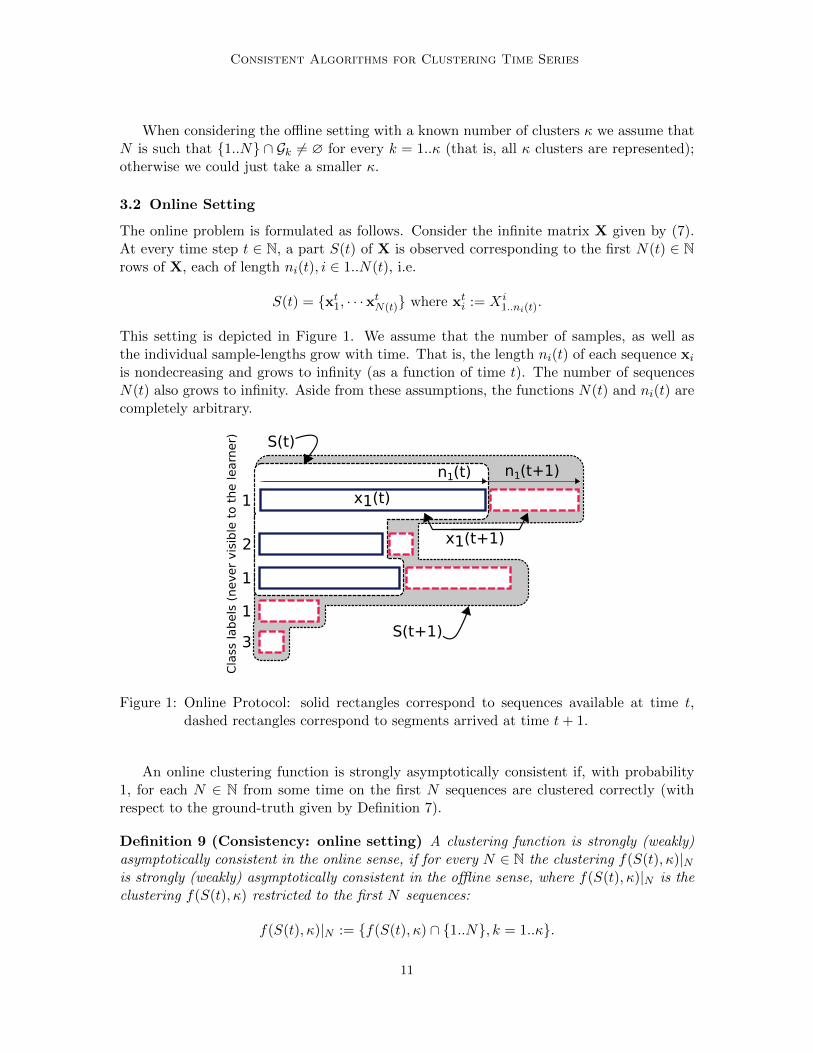
The online problem is formulated as follows. Consider the infinite matrix X given by (7).At every time step t ∈ N, a part S(t) of X is observed corresponding to the first N(t) ∈ Nrows of X, each of length ni(t), i ∈ 1..N(t), i.e.

S(t) = {xt1, · · ·xtN(t)} where xti := Xi1..ni(t)

.

This setting is depicted in Figure 1. We assume that the number of samples, as well asthe individual sample-lengths grow with time. That is, the length ni(t) of each sequence xiis nondecreasing and grows to infinity (as a function of time t). The number of sequencesN(t) also grows to infinity. Aside from these assumptions, the functions N(t) and ni(t) arecompletely arbitrary.

1

1

2

1

3

Cla

ss lab

els

(n

ever

vis

ible

to t

he learn

er)

n1(t+1)n1(t)

x1(t+1)

x1(t)

S(t)

S(t+1)

Figure 1: Online Protocol: solid rectangles correspond to sequences available at time t,dashed rectangles correspond to segments arrived at time t+ 1.

An online clustering function is strongly asymptotically consistent if, with probability1, for each N ∈ N from some time on the first N sequences are clustered correctly (withrespect to the ground-truth given by Definition 7).

Definition 9 (Consistency: online setting) A clustering function is strongly (weakly)asymptotically consistent in the online sense, if for every N ∈ N the clustering f(S(t), κ)|Nis strongly (weakly) asymptotically consistent in the offline sense, where f(S(t), κ)|N is theclustering f(S(t), κ) restricted to the first N sequences:

f(S(t), κ)|N := {f(S(t), κ) ∩ {1..N}, k = 1..κ}.

11


Remark 10 Note that even if the eventual number κ of different time-series distributionsproducing the sequences (that is, the number of clusters in the ground-truth clustering G)is known, the number of observed distributions at each individual time step is unknown.That is, it is possible that at a given time t we have

∣∣G|N(t)

∣∣ < κ.

Known and unknown κ. As mentioned in the introduction, in the general framework de-scribed above, consistent clustering (for both the offline and the online problems) withunknown number of clusters is impossible. This follows from the impossibility result ofRyabko (2010c) that states that when we have only two (binary-valued) samples generated(independently) by two stationary ergodic distributions, it is impossible to decide whetherthey have been generated by the same or by different distributions, even in the sense ofweak asymptotic consistency. (This holds even if the distributions come from a smallerclass: the set of all B-processes.) Therefore, if the number of clusters is unknown, we arebound to make stronger assumptions. Since our main interest in this paper is to developconsistent clustering algorithms under the general framework described above, for the mostpart of this paper we assume that the correct number κ of clusters is known. However, inSection 4.3 we also show that under certain mixing conditions on the process distributionsthat generate the data, it is possible to have consistent algorithms in the case of unknownκ as well.

4. Clustering Algorithms and their Consistency

In this section we present our clustering methods for both the offline and the online settings.The main results, presented in Sections 4.1 (offline) and 4.2 (online), concern the case wherethe number of clusters κ is known. In Section 4.3 we show that, given the mixing rates ofthe process distributions that generate the data, it is possible to find the correct number ofclusters κ and thus obtain consistent algorithms for the case of unknown κ as well. Finally,Section 4.4 considers some extensions of the proposed settings.

4.1 Offline Setting

Given that we have asymptotically consistent estimates d of the distributional distanced, it is relatively simple to construct asymptotically consistent clustering algorithms forthe offline setting. This follows from the fact that, since d(·, ·) converges to d(·, ·), forlarge enough sequence lengths n the points x1, . . . ,xN have the so-called strict separationproperty: the points within each target cluster are closer to each other than to points in anyother cluster (on strict separation in clustering see, for example, Balcan et al., 2008). Thismakes many simple algorithms, such as single or average linkage, or the k-means algorithmwith certain initialisations, provably consistent.

We present below one specific algorithm that we show to be asymptotically consistentin the general framework introduced. What makes this simple algorithm interesting is thatit requires only κN distance calculations (that is, much less than is needed to calculate thedistance between each two sequences). In short, Algorithm 1 initialises the clusters usingfarthest-point initialisation, and then assigns each remaining point to the nearest cluster.More precisely, the sample x1 is assigned as the first cluster centre. Then a sample is foundthat is farthest away from x1 in the empirical distributional distance d and is assigned as

12


the second cluster centre. For each k = 2..κ the kth cluster centre is sought as the sequencewith the largest minimum distance from the already assigned cluster centres for 1..k − 1.(This initialisation was proposed for use with k-means clustering by Katsavounidis et al.,1994.) By the last iteration we have κ cluster centres. Next, the remaining samples areeach assigned to the closest cluster.

Algorithm 1 Offline clustering

1: INPUT: sequences S := {x1, · · · ,xN}, Number κ of clusters2: Initialize κ-farthest points as cluster-centres:3: c1 ← 14: C1 ← {c1}5: for k = 2..κ do6: ck ← argmax

i=1..Nmin

j=1..k−1d(xi,xcj ), where ties are broken arbitrarily

7: Ck ← {ck}8: end for9: Assign the remaining points to closest centres:

10: for i = 1..N do11: k ← argminj∈

⋃κk=1 Ck

d(xi,xj)12: Ck ← Ck ∪ {i}13: end for14: OUTPUT: clusters C1, C2, · · · , Cκ

Theorem 11 Algorithm 1 is strongly asymptotically consistent (in the offline sense of Def-inition 8), provided that the correct number κ of clusters is known, and the marginal distri-bution of each sequence xi, i = 1..N is stationary ergodic.

Proof To prove the consistency statement we use Lemma 5 to show that if the samplesin S are long enough, the samples that are generated by the same process distributionare closer to each other than to the rest of the samples. Therefore, the samples chosen ascluster centres are each generated by a different process distribution, and since the algorithmassigns the rest of the samples to the closest clusters, the statement follows. More formally,let n denote the shortest sample length in S:

nmin := mini∈1..N

ni.

Denote by δ the minimum nonzero distance between the process distributions:

δ := mink 6=k′∈1..κ

d(ρk, ρk′).

Fix ε ∈ (0, δ/4). Since there are a finite number N of samples, by Lemma 5 for all largeenough nmin we have

supk∈1..κ

i∈Gk∩{1..N}

d(xi, ρk) ≤ ε. (8)

13


where Gk, k = 1..κ denote the ground-truth partitions given by Definition 7. By (8) andapplying the triangle inequality we obtain

supk∈1..κ

i,j∈Gk∩{1..N}

d(xi,xj) ≤ 2ε. (9)

Thus, for all large enough nmin we have

infi∈Gk∩{1..N}j∈Gk′∩{1..N}k 6=k′∈1..κ

d(xi,xj) ≥ infi∈Gk∩{1..N}j∈Gk′∩{1..N}k 6=k′∈1..κ

d(ρk, ρk′)− d(xi, ρk)− d(xj , ρk′)

≥ δ − 2ε (10)

where the first inequality follows from the triangle inequality, and the second inequalityfollows from (8) and the definition of δ. In words, (9) and (10) mean that the samples inS that are generated by the same process distribution are closer to each other than to therest of the samples. Finally, for all nmin large enough to have (9) and (10) we obtain

maxi=1..N

mink=1..κ−1

d(xi,xck) ≥ δ − 2ε > δ/2

where as specified by Algorithm 1, c1 := 1 and ck := argmaxi=1..N

minj=1..k−1

d(xi,xcj ), k = 2..κ.

Hence, the indices c1, . . . , cκ will be chosen to index sequences generated by different pro-cess distributions. To derive the consistency statement, it remains to note that, by (9) and(10), each remaining sequence will be assigned to the cluster centre corresponding to thesequence generated by the same distribution.

4.2 Online Setting

The online version of the problem turns out to be more complicated than the offline one. Thechallenge is that, since new sequences arrive (potentially) at every time step, we can neverrely on the distance estimates corresponding to all of the observed samples to be correct.Thus, as mentioned in the introduction, the main challenge can be identified with what weregard as “bad” sequences: recently-observed sequences, for which sufficient informationhas not yet been collected, and for which the estimates of the distance (with respect to anyother sequence) are bound to be misleading. Thus, in particular, farthest-point initialisationwould not work in this case. More generally, using any batch algorithm on all available dataat every time step results in not only mis-clustering “bad” sequences, but also in clusteringincorrectly those for which sufficient data are already available.

The solution, realised in Algorithm 2, is based on a weighted combination of severalclusterings, each obtained by running the offline algorithm (Algorithm 1) on different por-tions of data. The clusterings are combined with weights that depend on the batch sizeand on the minimum inter-cluster distance. This last step of combining multiple clusteringswith weights may be reminiscent of prediction with expert advice (see Cesa-Bianchi andLugosi, 2006 for an overview), where experts are combined based on their past performance.

14


Algorithm 2 Online Clustering

1: INPUT: Number κ of target clusters2: for t = 1..∞ do3: Obtain new sequences S(t) = {xt1, · · · ,xtN(t)}4: Initialize the normalization factor: η ← 05: Initialize the final clusters: Ck(t)← ∅, k = 1..κ6: Generate N(t)− κ+ 1 candidate cluster centres:7: for j = κ..N(t) do8: {Cj1 , . . . , C

jκ} ← Alg1({xt1, · · · ,xtj}, κ)

9: µk ← min{i ∈ Cjk}, k = 1..κ . Set the smallest index as cluster centre.

10: (cj1, . . . , cjκ)← sort(µ1, . . . , µκ) . Sort the cluster centres increasingly.

11: γj ← mink 6=k′∈1..κ d(xtcjk,xt

cjk′

) . Calculate performance score.

12: wj ← 1/j(j + 1)13: η ← η + wjγj14: end for15: Assign points to clusters:16: for i = 1..N(t) do

17: k ← argmink′∈1..κ1η

∑N(t)j=1 wjγj d(xti,x

tcjk′

)

18: Ck(t)← Ck(t) ∪ {i}19: end for20: OUTPUT: {C1(t), · · · , Ck(t)}21: end for

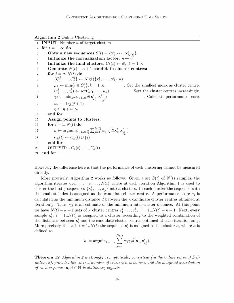
However, the difference here is that the performance of each clustering cannot be measureddirectly.

More precisely, Algorithm 2 works as follows. Given a set S(t) of N(t) samples, thealgorithm iterates over j := κ, . . . , N(t) where at each iteration Algorithm 1 is used tocluster the first j sequences {xt1, . . . ,xtj} into κ clusters. In each cluster the sequence withthe smallest index is assigned as the candidate cluster centre. A performance score γj is

calculated as the minimum distance d between the κ candidate cluster centres obtained atiteration j. Thus, γj is an estimate of the minimum inter-cluster distance. At this point

we have N(t)− κ + 1 sets of κ cluster centres cj1, . . . , cjκ, j = 1..N(t)− κ + 1. Next, every

sample xti, i = 1..N(t) is assigned to a cluster, according to the weighted combination ofthe distances between xti and the candidate cluster centres obtained at each iteration on j.More precisely, for each i = 1..N(t) the sequence xti is assigned to the cluster κ, where κ isdefined as

k := argmink=1..κ

N(t)∑j=κ

wjγj d(xti,xtcjk

).

Theorem 12 Algorithm 2 is strongly asymptotically consistent (in the online sense of Def-inition 9), provided the correct number of clusters κ is known, and the marginal distributionof each sequence xi, i ∈ N is stationary ergodic.

15


Before giving the proof of Theorem 12, we provide an intuitive explanation as to howAlgorithm 2 works. First, consider the following simple candidate solution. Take some fixed(reference) portion of the samples, run the batch algorithm on it, and then simply assignevery remaining sequence to the nearest cluster. Since the offline algorithm is asymptoticallyconsistent, this procedure would be asymptotically consistent as well, but only if we knewthat the selected reference of the sequences contains at least one sequence sampled fromeach and every one of the κ distributions. However, there is no way to find a fixed (notgrowing with time) portion of data that would be guaranteed to contain a representativeof each cluster (that is, of each time-series distribution). Allowing such a reference set ofsequences to grow with time would guarantee that eventually it contains representatives ofall clusters, but it would break the consistency guarantee for the reference set; since the setgrows, this formulation effectively returns us back to the original online clustering problem.

A key observation we make to circumvent this problem is the following. If, for somej ∈ {κ, . . . , N(t)}, each sample in the batch {xt1, . . . ,xtj} is generated by at most κ − 1process distributions, any partitioning of this batch into κ sets results in a minimum inter-cluster distance γj that, as follows from the asymptotic consistency of d, converges to 0.On the other hand, if the set of samples {xt1, . . . ,xtj} contains sequences generated by allκ process distributions, γj converges to a nonzero constant, namely, the minimum distancebetween the distinct process distributions ρ1, . . . , ρκ. In the latter case from some time onthe batch {xt1, . . . ,xtj} will be clustered correctly. Thus, instead of selecting one referencebatch of sequences and constructing a set of clusters based on those, we consider all batchesof sequences for j = κ..N(t), and combine them with weights. Two sets of weights areinvolved in this step: γj and wj , where

1. γj is used to penalise for small inter-cluster distance, cancelling the clustering resultsproduced based on sets of sequences generated by less than κ distributions;

2. wj is used to give precedence to chronologically earlier clusterings, protecting the clus-tering decisions from the presence of the (potentially “bad”) newly formed sequences,whose corresponding distance estimates may still be far from accurate.

As time goes on, the batches in which not all clusters are represented will have their weightγj converge to 0, while the number of batches that have all clusters represented and areclustered correctly by the offline algorithm will go to infinity, and their total weight willapproach 1. Note that, since we are combining different clusterings, it is important touse a consistent ordering of clusters, for otherwise we might sum up clusters generated bydifferent distributions. Therefore, we always order the clusters with respect to the index ofthe first sequence in each cluster.Proof [of Theorem 12] First, we show that for every k ∈ 1..κ we have

1

η

N(t)∑j=1

wjγtj d(xt

cjk, ρk)→ 0 a.s. (11)

Denote by δ the minimum nonzero distance between the process distributions:

δ := mink 6=k′∈1..κ

d(ρk, ρk′). (12)

16


Fix ε ∈ (0, δ/4). We can find an index J such that∑∞

j=J wj ≤ ε. Let S(t)|j = {xt1, · · · ,xtj}denote the subset of S(t) consisting of the first j sequences for j ∈ 1..N(t). For k = 1..κ let

sk := min{i ∈ Gk ∩ 1..N(t)} (13)

index the first sequence in S(t) that is generated by ρk where Gk, k = 1..κ are the ground-truth partitions given by Definition 7. Define

m := maxk∈1..κ

sk. (14)

Recall that the sequence lengths ni(t) grow with time. Therefore, by Lemma 5 (consistencyof d) for every j ∈ 1..J there exists some T1(j) such that for all t ≥ T1(j) we have

supk∈1..κ

i∈Gk∩{1..j}

d(xti, ρk) ≤ ε. (15)

Moreover, by Theorem 11 for every j ∈ m..J there exists some T2(j) such that Alg1(S(t)|j , κ)is consistent for all t ≥ T2(j). Let

T := maxi=1,2j∈1..J

Ti(j).

Recall that, by definition (14) of m, S(t)|m contains samples from all κ distributions. There-fore, for all t ≥ T we have

infk 6=k′∈1..κ

d(xtcmk,xtcm

k′) ≥ inf

k 6=k′∈1..κd(ρk, ρk′)− sup

k 6=k′∈1..κ(d(xtcmk

, ρk) + d(xtcmk′, ρk′))

≥ δ − 2ε ≥ δ/2, (16)

where the first inequality follows from the triangle inequality and the second inequalityfollows from the consistency of Alg1(S(t)|m, κ) for t ≥ T , the definition of δ given by (12)and the assumption that ε ∈ (0, δ/4). Recall that (as specified in Algorithm 2) we have

η :=∑N(t)

j=1 wjγtj . Hence, by (16) for all t ≥ T we have

η ≥ wmδ/2. (17)

By (17) and noting that by definition, d(·, ·) ≤ 1 for all t ≥ T , for every k ∈ 1..κ we obtain

1

η

N(t)∑j=1

wjγtj d(xt

cjk, ρk) ≤

1

η

J∑j=1

wjγtj d(xt

cjk, ρk) +

2ε

wmδ. (18)

On the other hand, by the definition (14) of m, the sequences in S(t)|j for j = 1..m− 1 aregenerated by at most κ− 1 out of the κ process distributions. Therefore, at every iterationon j ∈ 1..m−1 there exists at least one pair of distinct cluster centres that are generated bythe same process distribution. Therefore, by (15) and (17), for all t ≥ T and every k ∈ 1..κwe have,

1

η

m−1∑j=1

wjγtj d(xt

cjk, ρi) ≤

1

η

m−1∑j=1

wjγtj ≤

2ε

wmδ. (19)

17


Noting that the clusters are ordered in the order of appearance of the distributions, we havextcjk

= xtsk for all j = m..J and k = 1..κ, where the index sk is defined by (13). Therefore,

by (15) for all t ≥ T and every k = 1..κ we have

1

η

J∑j=m

wjγtj d(xt

cjk, ρk) =

1

ηd(xtsk , ρk)

J∑j=m

wjγtj ≤ ε. (20)

Combining (18), (19), and (20) we obtain

1

η

N(t)∑j=1

wjγtj d(xt

cjk, ρk) ≤ ε(1 +

4

wmδ). (21)

for all k = 1..κ and all t ≥ T , establishing (11).To finish the proof of the consistency, consider an index i ∈ Gr for some r ∈ 1..κ. By

Lemma 5, increasing T if necessary, for all t ≥ T we have

supk∈1..κ

j∈Gk∩1..N

d(xtj , ρk) ≤ ε. (22)

For all t ≥ T and all k 6= r ∈ 1..κ we have,

1

η

N(t)∑j=1

wjγtj d(xti,x

tcjk

) ≥ 1

η

N(t)∑j=1

wjγtj d(xti, ρk)−

1

η

N(t)∑j=1

wjγtj d(xt

cjk, ρk)

≥ 1

η

N(t)∑j=1

wjγtj(d(ρk, ρr)− d(xti, ρr))−

1

η

N(t)∑j=1

wjγtj d(xt

cjk, ρk)

≥ δ − 2ε(1 +2

wmδ), (23)

where the first and second inequalities follow from the triangle inequality, and the lastinequality follows from (22), (21) and the definition of δ. Since the choice of ε is arbitrary,from (22) and (23) we obtain

argmink∈1..κ

1

η

N(t)∑j=1

wjγtj d(xti,x

tcjk

) = r. (24)

It remains to note that for any fixed N ∈ N from some t on (24) holds for all i = 1..N , andthe consistency statement follows.

4.3 Unknown Number κ of Clusters

So far we have shown that when κ is known in advance, consistent clustering is possi-ble under the only assumption that the samples are generated by unknown stationary er-godic process distributions. However, as follows from the theoretical impossibility results

18


of Ryabko (2010c) discussed in Section 3, the correct number κ of clusters is not possible tobe estimated with no further assumptions or additional constraints. One way to overcomethis obstacle is to assume known rates of convergence of frequencies to the correspondingprobabilities. Such rates are provided by assumptions on the mixing rates of the processdistributions that generate the data.

Here we will show that under some assumptions on the mixing rates (and still withoutmaking any modelling or independence assumptions), consistent clustering is possible whenthe number of clusters is unknown.

The purpose of this section, however, is not to find the weakest assumptions underwhich consistent clustering (with κ unknown) is possible, nor is it to provide sharp boundsunder the assumptions considered; our only purpose here is to demonstrate that asymptoticconsistency is achievable in principle when the number of clusters is unknown, under somemild nonparametric assumptions on the time-series distributions. More refined analysiscould yield sharper bounds under weaker assumptions, such as those in, for example, (Bosq,1996; Rio, 1999; Doukhan, 1994; Doukhan et al., 2010).

We introduce mixing coefficients, mainly following Rio (1999) in formulations. Infor-mally, mixing coefficients of a stochastic process measure how fast the process forgets aboutits past. Any one-way infinite stationary process X1, X2, . . . can be extended backwardsto make a two-way infinite process . . . , X−1, X0, X1, . . . with the same distribution. In thedefinition below we assume such an extension. Define the ϕ-mixing coefficients of a processµ as

ϕn(µ) = supA∈σ(X−∞..k),B∈σ(Xk+n..∞),µ(A)6=0

|µ(B|A)− µ(B)|, (25)

where σ(..) stands for the σ-algebra generated by random variables in brackets. Thesecoefficients are nonincreasing. Define also

θn(µ) := 2 + 8(ϕ1(µ) + · · ·+ ϕn(µ)).

A process µ is called uniformly ϕ-mixing if ϕn(µ)→ 0. Many important classes of processessatisfy mixing conditions. For example, a stationary irreducible aperiodic Hidden Markovprocess with finitely many states is uniformly ϕ-mixing with coefficients decreasing expo-nentially fast. Other probabilistic assumptions can be used to obtain bounds on the mixingcoefficients, see, e.g., (Bradley, 2005) and references therein.

The method that we propose for clustering mixing time series in the offline setting,namely Algorithm 3, is very simple. Its inputs are: a set S := {x1, . . . ,xN} of samples eachof length ni, i = 1..N , the threshold level δ ∈ (0, 1) and the parameters m, l ∈ N, Bm,l,n.The algorithm assigns to the same cluster all samples which are at most δ-far from eachother, as measured by d with mn = m, ln = l and the summation over Bm,l restricted toBm,l,n. The sets Bm,l,n have to be chosen so that in asymptotic they cover the whole space,∪n∈NBm,l,n = Bm,l. For example, Bm,l,n may consist of the first bn cubes around the origin,where bn → ∞ is a parameter sequence. We do not give a pseudocode implementation ofthis algorithm, since it is rather clear.

The idea is that the threshold level δ = δn is selected according to the smallest sample-length n := mini=1..N ni and the (known bounds on) mixing rates of the process ρ generatingthe samples (see Theorem 13). As we show in Theorem 13, if the distribution of the samplessatisfies ϕn(ρ) ≤ ϕn → 0, where ϕn are known, then one can select (based on ϕn only)

19


the parameters of Algorithm 3 in such a way that it is weakly asymptotically consistent.Moreover, a bound on the probability of error before asymptotic is provided.

Theorem 13 (Algorithm 3 is consistent for unknown κ) Fix sequences mn, ln, bn ∈N, and let, for each m, l ∈ N, Bm,l,n ⊂ Bm,l be an increasing sequence of finite sets suchthat ∪n∈NBm,l,n = Bm,l. Set bn := maxl≤ln,m≤mn |Bm,l,n| and n := mini=1..N ni. Let alsoδn ∈ (0, 1). Let N ∈ N, and suppose that the samples x1, . . . ,xN are generated in sucha way that the (unknown marginal) distributions ρk, k = 1..κ are stationary ergodic andsatisfy ϕn(ρk) ≤ ϕn, for all k = 1..κ, n ∈ N. Then there exist constants ερ, δρ and nρ thatdepend only on ρk, k = 1..κ, such that for all δn < δρ and n > nρ, Algorithm 3 satisfies

P (T 6= G|N ) ≤ 2N(N + 1)(mnlnbnγn/2(δn) + γn/2(ερ)) (26)

where

γn(ε) :=√e exp(−nε2/θn),

T is the partition output by the algorithm and G|N is the ground-truth clustering. In partic-ular, if ϕn = o(1), then, selecting the parameters in such a way that δn = o(1), mn, ln, bn =

o(n), mn, ln → ∞, ∪k∈NBm,l,k = Bm,l, bm,ln → ∞, for all m, l ∈ N, γn(const) = o(1), and,finally, mnlnbnγn(δn) = o(1), as is always possible, Algorithm 3 is weakly asymptoticallyconsistent (with the number of clusters κ unknown).

Proof We use the following bound from (Rio, 1999, Corollary 2.1): for any zero-mean[−1, 1]-valued random process Y1, Y2, . . . with distribution P and every n ∈ N we have

P

(|n∑i=1

Yi| > nε

)≤ γn(ε). (27)

For every j = 1..N , every m < n, l ∈ N, and B ∈ Bm,l, define the [−1, 1]-valued processesYj := Y j

1 , Yj

2 , . . . as

Y jt := I{(Xj

t , . . . , Xjt+m−1) ∈ B} − ρk(Xj

1..m ∈ B),

where ρk is the marginal distribution of Xj (that is, k is such that j ∈ Gk). It is easy tosee that ϕ-mixing coefficients for this process satisfy ϕn(Yj) ≤ ϕn−2m. Thus, from (27) wehave

P (|ν(Xj1..nj

, B)− ρk(Xj1..m ∈ B)| > ε/2) ≤ γn−2mn(ε/2). (28)

Then for every i, j ∈ Gk ∩ 1..N for some k ∈ 1..κ (that is, xi and xj are in the sameground-truth cluster) we have

P (|ν(Xi1..ni , B)− ν(Xj

1..nj, B)| > ε) ≤ 2γn−2mn(ε/2).

Using the union bound, summing over m, l, and B, we obtain

P (d(xi,xj) > ε) ≤ 2mnlnbnγn−2mn(ε/2). (29)

20


Next, let i ∈ Gk ∩ 1..N and j ∈ Gk′ ∩ 1..N for k 6= k′ ∈ 1..κ (i.e., xi,xj are in two differenttarget clusters). Then, for some mi,j , li,j ∈ N there is Bi,j ∈ Bmi,j ,li,j such that for someτi,j > 0 we have

|ρk(Xi1..|Bi,j | ∈ Bi,j)− ρk′(X

j1..|Bi,j | ∈ Bi,j)| > 2τi,j .

Then for every ε < τi,j/2 we have

P (|ν(Xi1..ni , Bi,j)− ν(Xj

1..nj, Bi,j)| < ε) ≤ 2γn−2mi,j (τi,j). (30)

Moreover, for ε < wmi,jwli,jτi,j/2 we have

P (d(xi,xj) < ε) ≤ 2γn−2mi,j (τi,j). (31)

Defineδρ := min

k 6=k′∈1..κi∈Gk∩1..Nj∈Gk′∩1..N

wmi,jwli,jτi,j/2, ερ := mink 6=k′∈1..κi∈Gk∩1..Nj∈Gk′∩1..N

τi,j/2

nρ := 2 maxk 6=k′∈1..κi∈Gk∩1..Nj∈Gk′∩1..N

mi,j .

Clearly, from this and (30), for every δ < 2δρ and n > nρ we obtain

P (d(xi,xj) < δ) ≤ 2γn/2(ερ). (32)

Algorithm 3 produces correct results if for every pair i, j we have d(xi,xj) < δn if and onlyif i, j ∈ Gk ∩ 1..N for some k ∈ 1..κ. Therefore, taking the bounds (29) and (32) togetherfor each of the N(N + 1)/2 pairs of samples, we obtain (26).

For the online setting, consider the following simple extension of Algorithm 3, that wecall Algorithm 3’. It applies Algorithm 3 to the first Nt sequences, where the parametersof Algorithm 3 and Nt are chosen in such a way that the bound (26) with N = Nt is o(1)and Nt → ∞ as time t goes to infinity. It then assigns each of the remaining sequences(xi, i > Nt) to the nearest cluster. Note that in this case the bound (26) with N = Nt

bounds the error of Algorithm 3’ on the first Nt sequences, as long as all of the κ clustersare already represented among the first Nt sequences. Since Nt →∞, we can formulate thefollowing result.

Theorem 14 Algorithm 3’ is weakly asymptotically consistent in the online setting whenthe number κ of clusters is unknown, provided that the assumptions of Theorem 13 apply tothe first N sequences x1, . . . ,xN for every N ∈ N.

4.4 Extensions

In this section we show that some simple, yet rather general extensions of the main resultsof this paper are possible, namely allowing for non-stationarity and for slight differences indistributions in the same cluster.

21


4.4.1 AMS Processes and Gradual Changes

Here we argue that our results can be strengthened to a more general case where theprocess distributions that generate the data are Asymptotically Mean Stationary (AMS)ergodic. Throughout the paper we have been concerned with stationary ergodic processdistributions. Recall from Section 2 that a process ρ is stationary if for any i, j ∈ 1..nand B ∈ Bm, m ∈ N, we have ρ(X1..j ∈ B) = ρ(Xi..i+j−1 ∈ B). A stationary processis called ergodic if the limiting frequencies converge to their corresponding probabilities,so that for all B ∈ B with probability 1 we have limn→∞ ν(X1..n, B) = ρ(B). This latterconvergence of all frequencies is the only property of the process distributions that is usedin the proofs (via Lemma 5) which give rise to our consistency results. We observe thatthis property also holds for a more general class of processes, namely those that are AMSergodic. Specifically, a process ρ is called AMS if for every j ∈ 1..n and B ∈ Bm,m N theseries limn→∞

∑n−j+1i=1

1nρ(Xi..i+j−1 ∈ B) converges to a limit ρ(B), which forms a measure,

i.e. ρ(X1..j ∈ B) := ρ(B), B ∈ Bm, m ∈ N, called asymptotic mean of ρ. Moreover, if ρ isan AMS process, then for every B ∈ Bm, m ∈ N, the frequency ν(X1..n, B) converges ρ-a.s.to a random variable with mean ρ(B). Similarly to stationary processes, if the randomvariable to which ν(X1..n, B) converges is a.s. constant, then ρ is called AMS ergodic. Moreinformation on AMS processes can be found in the work (Gray, 1988). However, the maincharacteristic pertaining to our work is that the class of all processes with AMS properties iscomposed precisely of those processes for which the almost sure convergence of frequenciesto the corresponding probabilities holds. It is thus easy to check that all of the asymptoticresults of Sections 4.1, 4.2 carry over to the more general setting where the unknown processdistributions that generate the data are AMS ergodic.

4.4.2 Strictly Separated Clusters of Distributions

So far we have defined a cluster as a set of sequences generated by the same distribution.This seems to capture rather well the notion that in the same cluster the objects can bevery different (as is the case for stochastically generated sequences), yet are intrinsically ofthe same nature (they have the same law).

However, one may wish to generalise this further, and allow each sequence to be gener-ated by a different distribution, yet requiring that in the same clusters distributions mustbe close. Unlike the original formulation, such an extension would require fixing some sim-ilarity measure between distributions. The results of the preceding sections suggest usingthe distributional distance for this purpose.

Specifically, as discussed in Section 4.1, in our formulation, from some time on, thesequences possess the so-called strict separation property in the d distance: sequences inthe same target cluster are closer to each other than to those in other clusters. One possibleway to relax the considered setting is to impose the strict separation property on thedistributions that generate the data. Here the separation would be with respect to thedistributional distance d. That is, each sequence xi, i = 1..N , may be generated by its owndistribution ρi, but the distributions {ρi : i = 1..N} can be clustered in such a way that theresulting clustering has the strict separation property with respect to d. The goal wouldthen be to recover this clustering based on the given samples. In fact, it can be shown thatthe offline Algorithm 1 of Section 4.1 is consistent in this setting as well. How this transfers

22


to the online setting remains open. For the offline case, we can formulate the followingresult, whose proof is analogous to that of Theorem 11.

Theorem 15 Assume that each sequence xi, i = 1..N is generated by a stationary ergodicdistribution ρi. Assume further that the set of distributions {1, . . . , N} admits a parti-tioning G = {G1, . . . ,Gk} that has the strict separation property with respect to d: for alli, j = 1..k, i 6= j, for all ρ1, ρ2 ∈ Gi and all ρ3 ∈ Gj we have d(ρ1, ρ2) < d(ρ1, ρ3). ThenAlgorithm 1 is strongly asymptotically consistent, in the sense that almost surely from somen = min{n1, . . . , nN} on it outputs the set G.

5. Computational Considerations

In this section we show that all of the proposed methods are efficiently computable. Thisclaim is further illustrated by the experimental results in the next section. Note, however,that since the results presented are asymptotic, the question of what is the best achievablecomputational complexity of an algorithm that still has the same asymptotic performanceguarantees is meaningless: for example, an algorithm could throw away most of the data andstill be asymptotically consistent. This is why we do not attempt to find a resource-optimalway of computing the methods presented.First, we show that calculating d is at most quadratic (up to log terms), and quasilinearif we use mn = log n. Let us begin by showing that calculating d is fully tractable withmn, ln ≡ ∞. First, observe that for fixed m and l, the sum

Tm,l :=∑

B∈Bm,l|ν(X1

1..n1, B)− ν(X2

1..n2, B)| (33)

has not more than n1 + n2− 2m+ 2 nonzero terms (assuming m ≤ n1, n2; the other case isobvious). Indeed, there are ni−m+ 1 tuples of size m in each sequence xi, i = 1, 2 namely,Xi

1..m, Xi2..m+1, . . . , X

in1−m+1..n1

. Therefore, Tm,l can be obtained by a finite number ofcalculations.

Furthermore, let

s = minX1i 6=X2

j

i=1..n1,j=1..n2

|X1i −X2

j |, (34)

and observe that Tm,l = 0 for all m > n and for each m, for all l > log s−1 the term Tm,l

is constant. That is, for each fixed m we have

∞∑l=1

wmwlTm,l = wmwlog s−1Tm,log s−1

+

log s−1∑l=1

wmwlTm,l

so that we simply double the weight of the last nonzero term. (Note also that s is boundedabove by the length of the binary precision in representing the random variables Xi

j .) Thus,

even with mn, ln ≡ ∞ one can calculate d precisely. Moreover, for a fixed m ∈ 1.. log n andl ∈ 1.. log s−1 for every sequence xi, i = 1, 2 the frequencies ν(xi, B), B ∈ Bm,l maybe calculated using suffix trees or suffix arrays, with O(n) worst case construction andsearch complexity (see, e.g., Ukkonen, 1995). Searching all z := n −m + 1 occurrences of

23


subsequences of length m results in O(m + z) = O(n) complexity. This brings the overallcomputational complexity of (3) to O(nmn log s−1); this can potentially be improved usingspecialized structures, e.g., (Grossi and Vitter, 2005).

The following consideration can be used to set mn. For a fixed l the frequenciesν(xi, B), i = 1, 2 of cells in B ∈ Bm,l corresponding to values of m much larger than logn(in the asymptotic sense, that is, if logn = o(m)) are not, in general, consistent estimatesof their probabilities, and thus only add to the estimation error. More specifically, for asubsequence Xj..j+m with j = 1..n−m of length m the probability ρi(Xj..j+m ∈ B), i = 1, 2is of order 2−mhi , i = 1, 2 where hi denotes the entropy rate of ρi, i = 1, 2. Moreover, undersome (general) conditions (including hi > 0) one can show that, asymptotically, a string oflength of order log n/hi on average occurs at most once in a string of length n (Kontoyiannisand Suhov, 1994). Therefore, subsequences of length m larger than log n are typically met0 or 1 times, and thus are not consistent estimates of probabilities. By the above argument,one can use mn of order log n. To choose ln <∞ one can either fix some constant based onthe bound on the precision in real computations, or choose it in such a way that each cellBm,ln contains no more than log n points for all m = 1.. log n largest values of ln.

5.1 Complexity of the Algorithms.

The computational complexity of the presented algorithms is dominated by the complexityof calculations of d between different pairs of sequences. Thus, it is sufficient to bound thenumber of pairwise d computations.

It is easy to see that the offline algorithm for the case of known κ (Algorithm 1) re-quires at most κN distance calculations, while for the case of unknown κ all N2 distancecalculations are necessary.

The computational complexity of the updates in the online algorithm can be computedas follows. Assume that the pairwise distance values are stored in a database D, and thatfor every sequence xt−1

i , i ∈ N we have already constructed a suffix tree, using for example,the online algorithm of Ukkonen (1995). At time step t, a new symbol X is received. Letus first calculate the required computations to update D. We have two cases, either Xforms a new sequence, so that N(t) = N(t − 1) + 1, or it is the subsequent element of apreviously received segment, say, xtj for some j ∈ 1..N(t), so that nj(t) = nj(t − 1) + 1.In either case, let xtj denote the updated sequence. Note that for all i 6= j ∈ 1..N(t) we

have ni(t) = ni(t− 1). Recall the notation xti := X(i)1 , . . . X

(i)ni(t)

for i ∈ 1..N(t). In order to

update D we need to update the distance between xtj and xti for all i 6= j ∈ N(t). Thus,we need to search for all mn new patterns induced by the received symbol X, resulting incomplexity at most O(N(t)m2

nln). Let n(t) := max{n1(t), . . . nN(t)(t)}, t ∈ N. As discussedpreviously, we let mn := log n(t); we also define ln := log s(t)−1 where

s(t) := mini,j∈1..N(t)

u=1..ni(t),v=1..nj(t),X(i)u 6=X

(j)v

|X(i)u −X(j)

v |, t ∈ N.

Thus, the per symbol complexity of updating D is at most O(N(t) log3 n(t)). However, notethat if s(t) decreases from one time step to the next, updating D will have a complexity

24


of order equivalent to its complete construction, resulting in a computational complexityof order O(N(t)n(t) log2 n(t)). Therefore, we avoid calculating s(t) at every time step;instead, we update s(t) at prespecified time steps so that for every n(t) symbols received,D is reconstructed at most log n(t) times. (This can be done, for example, by recalculatings(t) at time steps where n(t) is a power of 2.) It is easy to see that with the database D ofdistance values at hand, the rest of the computations are of order at most O(N(t)2). Thus,the computational complexity of updates in Algorithm 2 is at mostO(N(t)2+N(t) log3 n(t)).

6. Experimental Results

In this section we present empirical evaluations of Algorithms 1 and 2 on both syntheticallygenerated and real data.

6.1 Synthetic Data

We start with synthetic experiments. In order for the experiments to reflect the generality ofour approach we have selected time-series distributions that, while being stationary ergodic,cannot be considered as part of any of the usual smaller classes of processes, and are difficultto approximate by finite-state models. Namely, we consider rotation processes used, forexample, by Shields (1996) as an example of stationary ergodic processes that are not B-processes. Such time series cannot be modelled by a hidden Markov model with a finiteor countably infinite set of states. Moreover, while k-order Markov (or hidden Markov)approximations of this process converge to it in the distributional distance d, they do notconverge to it in the d distance, a stronger distance than d whose empirical approximationsare often used to study general (non-Markovian) processes (e.g., Ornstein and Weiss, 1990).

6.1.1 Time Series Generation

To generate a sequence x = X1..n we proceed as follows: Fix some parameter α ∈ (0, 1).Select r0 ∈ [0, 1]; then, for each i = 1..n obtain ri by shifting ri−1 by α to the right, andremoving the integer part, i.e. ri := ri−1 + α− bri−1 + αc. The sequence x = (X1, X2, · · · )is then obtained from ri by thresholding at 0.5, that is Xi := I{ri > 0.5}. If α is irrationalthen x forms a stationary ergodic time series. (We simulate α by a longdouble with a longmantissa.)

For the purpose of our experiments, first we fix κ := 5 difference process distributionsspecified by α1 = 0.31..., α2 = 0.33..., α3 = 0.35..., α4 = 0.37..., α5 = 0.39.... The param-eters αi are intentionally selected to be close, in order to make the process distributionsharder to distinguish. Next we generate an N ×M data matrix X, each row of which isa sequence generated by one of the process distributions. Our task in both the online andthe batch setting is to cluster the rows of X into κ = 5 clusters.

6.1.2 Batch Setting

In this experiment we demonstrate that in the batch setting, the clustering errors corre-sponding to both the online and the offline algorithms converge to 0 as the sequence-lengthsgrow. To this end, at every time step t we take an N×n(t) submatrix X|n(t) of X composedof the rows of X terminated at length n(t), where n(t) = 5t. Then at each iteration we let

25


each of the algorithms, (online and offline) cluster the rows of X|n(t) into five clusters, andcalculate the clustering error rate of each algorithm. As shown in Figure 2 (top) the errorrate of each algorithm decreases with sequence length.

0 100 200 300 400

0.0

0.1

0.2

0.3

0.4

0.5

Timestep

MeanoftheErrorRate

OnlineOffline

Figure 2: Top: error rate vs. sequence length in batch setting. Bottom: error rate vs.Number of observed samples in online setting. (error rates averaged over 100runs.)

6.1.3 Online Setting

In this experiment we demonstrate that, unlike the online algorithm, the offline algorithm isconsistently confused by the new sequences arriving at each time step in an online setting.To simulate an online setting, we proceed as follows: At every time step t, a triangularwindow is used to reveal the first 1..ni(t), i = 1..t elements of the first t rows of the datamatrix X, with ni(t) := 5(t − i) + 1, i = 1..t. This gives a total of t sequences, each oflength ni(t), for i = 1..t, where the ith sequence for i = 1..t corresponds to the ith row of Xterminated at length ni(t). At every time step t the online and offline algorithms are eachused in turn to cluster the observed t sequences into five clusters. Note that the performance

26


of both algorithms is measured on all sequences available at a given time, not on a fixedbatch of sequences. As shown in Figure 2 (bottom), in this setting the clustering errorrate of the offline algorithm remains consistently high, whereas that of the online algorithmconverges to zero.

6.2 Real Data

As an application we consider the problem of clustering motion capture sequences, wheregroups of sequences with similar dynamics are to be identified. Data is taken from theMotion Capture database (MOCAP) which consists of time-series data representing humanlocomotion. The sequences are composed of marker positions on human body which aretracked spatially through time for various activities.

We compare our results to those obtained with two other methods, namely those of Liand Prakash (2011) and Jebara et al. (2007). Note that we have not implemented thesereference methods, rather we have taken the numerical results directly from the correspond-ing articles. In order to have common grounds for each comparison we use the same setsof sequences2 and the same means of evaluation as those used by Li and Prakash (2011);Jebara et al. (2007).

In the paper by Li and Prakash (2011) two MOCAP data sets3 are used, where thesequences in each data set are labelled with either running or walking as annotated in thedatabase. Performance is evaluated via the conditional entropy S of the true labellingwith respect to the prediction, i.e., S := −

∑i,j

Mij∑i′,j′Mi′j′

logMij∑j′Mij′

where M denotes

the clustering confusion matrix. The motion sequences used by Li and Prakash (2011) arereportedly trimmed to equal duration. However, we use the original sequences as our methodis not limited by variation in sequence lengths. Table 1 lists performance of Algorithm 1as well as that reported for the method of Li and Prakash (2011); Algorithm 1 performsconsistently better.

In the paper (Jebara et al., 2007) four MOCAP data sets4 are used, corresponding tofour motions: run, walk, jump and forward jump. Table 2 lists performance in terms ofaccuracy. The data sets in Table 2 constitute two types of motions:

1. motions that can be considered ergodic: walk, run, run/jog (displayed above thedouble line), and

2. non-ergodic motions: single jumps (displayed below the double line).

As shown in Table 2, Algorithm 1 achieves consistently better performance on the firstgroup of data sets, while being competitive (better on one and worse on the other) on thenon-ergodic motions. The time taken to complete each task is in the order of few minuteson a standard laptop computer.

2. The subject’s right foot was used as marker position.3. The corresponding subject references are #16 and #35.4. The corresponding subject references are #7, #9, #13, #16 and #35.

27


Data set (Li and Prakash, 2011) Algorithm 1

1. Walk vs. Run (#35) 0.1015 02. Walk vs. Run (#16) 0.3786 0.2109

Table 1: Comparison with the work (Li and Prakash, 2011): Performance in terms of en-tropy; data sets concern ergodic motion captures.

Data set (Jebara et al., 2007) Algorithm 1

1. Run(#9) vs. Run/Jog(#35) 100% 100%2. Walk(#7) vs. Run/Jog(#35) 95% 100%

3. Jump vs. Jump fwd.(#13) 87% 100%4. Jump vs. Jump fwd.(#13, 16) 66% 60%

Table 2: Comparison with the work (Jebara et al., 2007): Performance in terms of accuracy;Rows 1 & 2 concern ergodic, Rows 3 & 4 concern non-ergodic motion captures.

7. Discussion

We have proposed a natural notion of consistency for clustering time series in both the onlineand the offline settings. While in this work we have taken some first steps in investigatingthe theoretical and algorithmic questions arising in the proposed framework, there are manyopen problems and exciting directions for future research remaining to be explored. Someof these are discussed in this section.

Rates, optimality. The main focus of this work is on the most general case of highlydependent time series. On the one hand, this captures best the spirit of the unsupervisedlearning problem in question: the nature of the data is completely unknown, and one triesto find some structure in it. On the other hand, as discussed above, in this generality ratesof convergence and finite-sample performance guarantees are provably impossible to obtain,and thus one cannot argue about optimality. While we have provided some results on amore restrictive setting (time series with mixing, Section 4.3), the question of what theoptimal performance guarantees are for different classes of time series remains open. Infact, the first interesting question in this direction is not about time series with mixing, butabout i.i.d. series. What is the minimal achievable probability of clustering error in thissetting, for finite sample sizes, and what algorithms attain it?

Online setting: bad points. In the online setting of Section 4.2, we have assumed that thelength of each sequence grows to infinity with time. While this is a good first approximation,this assumption may not be practical. It is interesting to consider the situation in whichsome sequences stop growing at some point; moreover, it can be assumed that such sequencesare not representative of the corresponding distribution. While this clearly makes theproblem much more difficult, already in the setting considered in this work we have dealtwith “bad” sequences at each time step: these are those sequences which are as yet tooshort to be informative. This hints at the possibility of obtaining consistent algorithms inthe extended setting outlined.

Other metrics and non-metric-based methods. All of the methods presented in this paperare based on the distributional distance d. The main property of this distance that we

28


exploit is that it can be estimated consistently. In principle, one can use other distanceswith this property, in order to obtain consistent clustering algorithms. While there are notmany known distances that can be consistently estimated for arbitrary stationary ergodicdistributions, there is at least one, namely the telescope distance recently introduced byRyabko and Mary (2013). Moreover, the definition of consistency proposed does not entailthe need to use a distance between time-series distributions. As an alternative, the useof compression-based methods can be considered. Such methods have been used to solvevarious statistical problems concerning stationary ergodic time series (Ryabko and Astola,2006; Ryabko, 2010a). Compression-based methods have also been used for clustering time-series data before, albeit without consistency analysis, by Cilibrasi and Vitanyi (2005).Combining our consistency framework with these compression-based methods is anotherpromising direction for further research.

Acknowledgments

This paper is an extended version of two conference papers: (Ryabko, 2010b) and (Khaleghiet al., 2012). Most of the work by Azadeh Khaleghi has been done during her PhD at INRIALille - Nord Europe. This work is supported by the French Ministry of Higher Educationand Research, by FP7/2007-2013 under grant agreements 270327 (CompLACS), by theNord-Pas-de-Calais Regional Council and FEDER, and by the European Research Coun-cil (SMAC-ERC-280032). Jeremie Mary and Philippe Preux acknowledge the support ofINRIA. Jeremie Mary further acknowledges INRIA for the support through partial second-ments.

References

F.R. Bach and M.I. Jordan. Learning graphical models for stationary time series. IEEETransactions on Signal Processing, 52(8):2189 – 2199, Aug. 2004.

M.F. Balcan, A. Blum, and S. Vempala. A discriminative framework for clustering viasimilarity functions. In Proceedings of the 40th Annual ACM Symposium on Theory ofComputing, pages 671–680, 2008.

C. Biernacki, G. Celeux, and G. Govaert. Assessing a mixture model for clustering withthe integrated completed likelihood. Pattern Analysis and Machine Intelligence, IEEETransactions on, 22(7):719–725, 2000.

P. Billingsley. Statistical methods in Markov chains. The Annals of Mathematical Statistics,32(1):12–40, 1961.

P. Billingsley. Convergence of Probability Measures. John Wiley & Sons, 1999.

D. Bosq. Nonparametric Statistics for Stochastic Processes. Estimation and Prediction.Springer, 1996.

R.C. Bradley. Basic properties of strong mixing conditions: A survey and some openquestions. Probability Surveys, 2:107–144, 2005.

29


E. Carlstein and S. Lele. Nonparametric change-point estimation for data from an ergodicsequence. Theory of Probability & its Applications, 38(4):726–733, 1994.

N. Cesa-Bianchi and G. Lugosi. Prediction, Learning, and Games. Cambridge UniversityPress, 2006.

R. Cilibrasi and P.M.B. Vitanyi. Clustering by compression. IEEE Transactions on Infor-mation Theory, 51:1523–1545, 2005.

P. Doukhan. Mixing. Springer, 1994.

P. Doukhan, G. Lang, D. Surgailis, and G. Teyssiere. Dependence in Probability and Statis-tics. Springer, 2010.

R. Gray. Probability, Random Processes, and Ergodic Properties. Springer Verlag, 1988.

R. Grossi and J.S. Vitter. Compressed suffix arrays and suffix trees with applications totext indexing and string matching. SIAM Journal on Computing, 35(2):378–407, 2005.

M. Gutman. Asymptotically optimal classification for multiple tests with empirically ob-served statistics. IEEE Transactions on Information Theory, 35(2):402–408, 1989.

T. Jebara, Y. Song, and K. Thadani. Spectral clustering and embedding with hiddenMarkov models. Machine Learning: ECML 2007, pages 164–175, 2007.

I. Katsavounidis, C.-C. Jay Kuo, and Zhen Zhang. A new initialisation technique forgeneralised Lloyd iteration. IEEE Signal Processing Letters, 1:144–146, 1994.

A. Khaleghi and D. Ryabko. Locating changes in highly-dependent data with unknownnumber of change points. In Neural Information Processing Systems (NIPS), Lake Tahoe,Nevada, United States, 2012.

A. Khaleghi, D. Ryabko, J. Mary, and P. Preux. Online clustering of processes. In Interna-tional Conference on Artificial Intelligence and Statistics (AI&STATS), JMLR W&CP22, pages 601–609, 2012.

A. Khaleghi and D. Ryabko. Asymptotically consistent estimation of the number of changepoints in highly dependent time series. In the Proceedings of the 29th InternationalConference on Machine Learning (ICML), JMLR W&CP, pages 539–547, Beijing, China,2014.

J. Kleinberg. An impossibility theorem for clustering. In Neural Information ProcessingSystems (NIPS), pages 446–453, Montreal, Canada, 2002.

I. Kontoyiannis and Y.M. Suhov. Prefixes and the entropy rate for long-range sources. InIEEE International Symposium on Information Theory, pages 194–194, 1994.

M. Kumar, N.R. Patel, and J. Woo. Clustering seasonality patterns in the presence oferrors. In Proceedings of the 8th International Conference on Knowledge Discovery andData Mining (ACM SIGKDD), pages 557–563. ACM, 2002.

30


E. Lehmann. Testing Statistical Hypotheses, 2nd edition. Wiley, New York, 1986.

L. Li and B.A. Prakash. Time series clustering: Complex is simpler! In the Proceedings ofthe 28th International Conference on Machine Learning (ICML), pages 185–192, 2011.

M. Mahajan, P. Nimbhorkar, and K. Varadarajan. The planar k-means problem is NP-hard.In the Proceedings of the 3rd International Workshop on Algorithms and Computation(WALCOM), pages 274–285, Berlin, Heidelberg, 2009.

G. Morvai and B. Weiss. On classifying processes. Bernoulli, 11(3):523–532, 2005.

MOCAP. CMU graphics lab motion capture database. Available at http://mocap.cs.

cmu.edu/.

G. Morvai and B. Weiss. A note on prediction for discrete time series. Kybernetika, 48(4):809–823, 2012.

D.S. Ornstein and B. Weiss. How sampling reveals a process. Annals of Probability, 18(3):905–930, 1990.

E. Rio. Theorie asymptotique des processus aleatoires faiblement dependants, volume 31.Springer, 1999.

B. Ryabko. Prediction of random sequences and universal coding. Problems of InformationTransmission, 24:87–96, 1988.

B. Ryabko and J. Astola. Universal codes as a basis for time series testing. StatisticalMethodology, 3:375–397, 2006.

B. Ryabko. Applications of universal source coding to statistical analysis of time series.Selected Topics in Information and Coding Theory, World Scientific Publishing, pages289–338, 2010a.

D. Ryabko. Clustering processes. In the Proceedings of the 27th International Conferenceon Machine Learning (ICML), pages 919–926, Haifa, Israel, 2010b.

D. Ryabko. Discrimination between B-processes is impossible. Journal of Theoretical Prob-ability, 23(2):565–575, 2010c.

D. Ryabko. Testing composite hypotheses about discrete ergodic processes. Test, 21(2):317–329, 2012.

D. Ryabko. Uniform hypothesis testing for finite-valued stationary processes. Statistics, 48(1):121–128, 2014.

D. Ryabko and B. Ryabko. Nonparametric statistical inference for ergodic processes. IEEETransactions on Information Theory, 56(3):1430–1435, 2010.

D. Ryabko and J. Mary. A binary-classification-based metric between time-series distri-butions and its use in statistical and learning problems. Journal of Machine LearningResearch, 14:2837–2856, 2013.

31

http://mocap.cs.cmu.edu/

http://mocap.cs.cmu.edu/


P. Shields. The Ergodic Theory of Discrete Sample Paths. AMS Bookstore, 1996.

P. Smyth. Clustering sequences with hidden Markov models. In Advances in Neural Infor-mation Processing Systems, pages 648–654. MIT Press, 1997.

M. Tschannen and H. Bolcskei. Nonparametric nearest neighbor random process clustering.In Proceedings of the 2015 IEEE International Symposium on Information Theory, pages1207–1211, Hong Kong, 2015. IEEE.

E. Ukkonen. On-line construction of suffix trees. Algorithmica, 14(3):249–260, 1995.

S. Zhong and J. Ghosh. A unified framework for model-based clustering. Journal of MachineLearning Research, 4:1001–1037, 2003.

32

Consistent Algorithms for Clustering Time Serieskhaleghi/Publications_files/khaleghi16a.pdf ·...

Documents

Transcript of Consistent Algorithms for Clustering Time Serieskhaleghi/Publications_files/khaleghi16a.pdf ·...