Design and Analysis of Computer Experiments with

Qualitative and Quantitative Factors

Peter Z. G. Qian

Assistant Professor

Department of Statistics

University of Wisconsin-Madison

E-mail: peterq@stat.wisc.edu

1

Collaborators

• Huaiqin Wu, Iowa State University.

• Jeff Wu at Georgia Tech.

• Qiang Zhou and Shiyu Zhou, University of Wisconsin-Madison.

2

Outline

• Modeling computer experiments with qualitative and quantitative factors.

• Sliced space-filling designs.

3

Computer Experiments

• Computer experiments: experiments using complex mathematical models,

implemented in large computer codes, to study real physicalsystems. E.g.,

finite element analysis and computational fluid dynamics.

• Can be expensive to run.

• Noise and bias don’t occur indeterministiccomputer experiments,

at least not in the traditional way.

• Principles of Replication, Blocking and Randomization areirrelevant.

• Correlated inputs. “Gambling on tomorrow,” Aug 16th 2007,Economist.

• High-dimensional inputs.

• Complex responses.

4

Motivating Example : Data Center Thermal Management

From http://blogs.business2.com/greenwombat/2007/08/sun- greens-the-.html

Data Center Computer Experiment

•Based on computational fluid dynamics (CFD).• Implemented in Flotherm.• Each run takes hours to complete.

Gaussian Process (GP) Models with Quantitative

Factors

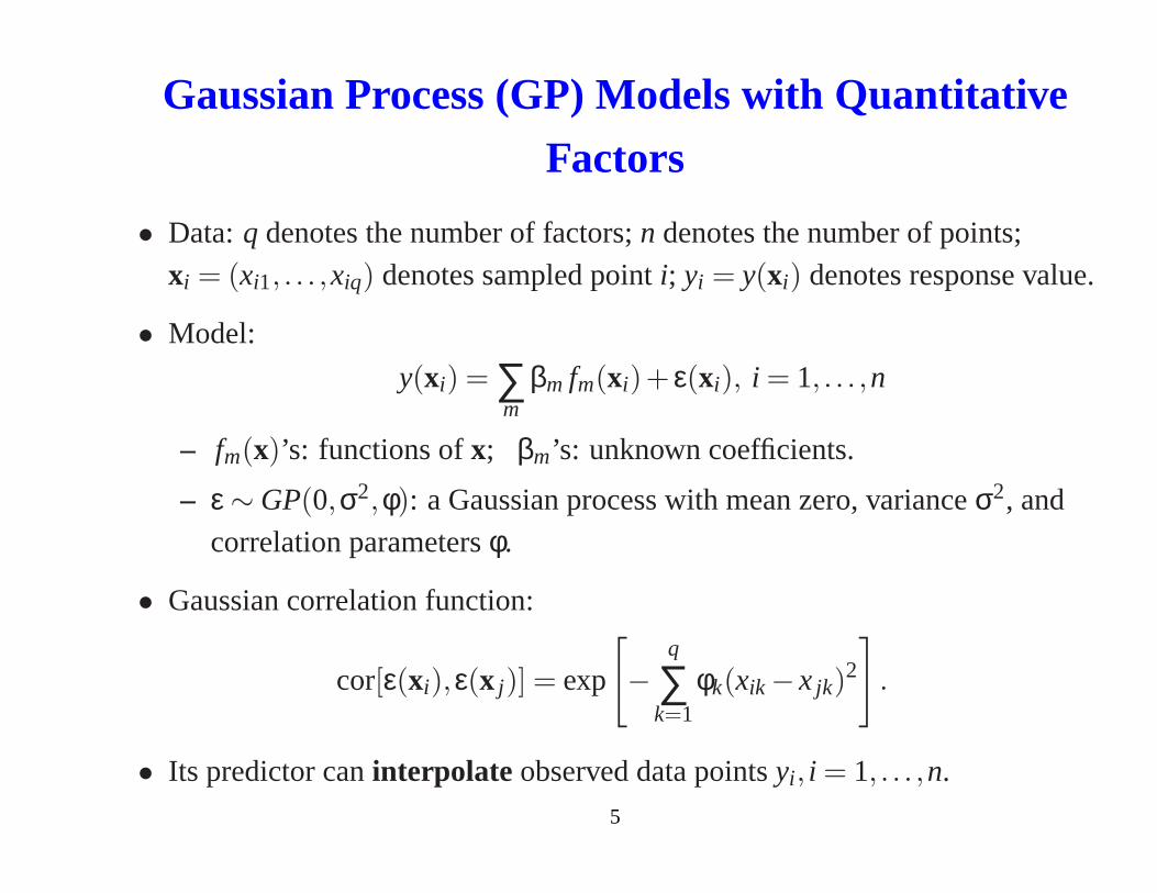
• Data:q denotes the number of factors;n denotes the number of points;

xi = (xi1, . . . ,xiq) denotes sampled pointi; yi = y(xi) denotes response value.

• Model:

y(xi) = ∑m

βm fm(xi)+ ε(xi), i = 1, . . . ,n

– fm(x)’s: functions ofx; βm’s: unknown coefficients.

– ε ∼ GP(0,σ2,φ): a Gaussian process with mean zero, varianceσ2, and

correlation parametersφ.

• Gaussian correlation function:

cor[ε(xi),ε(x j)] = exp

[−

q

∑k=1

φk(xik −x jk)2

].

• Its predictor caninterpolate observed data pointsyi , i = 1, . . . ,n.

5

Factors in the Data Center Example

• Quantitative factors include rack temperature rise, rack power, diffuser angle

and diffuser flow rate.

• Qualitative factors include diffuser type and cooling material type.

6

Two Naive Approaches for Modeling Quantitative and

Qualitative Factors

• Factors:w = (x,z); I quantitative factors:x = (x1, . . . ,xI ); J qualitative

factors:z = (z1, . . . ,zJ); response value:y(w).

• Independent Approach: fitting distinct GPs to data at different level

combinations ofz.

Drawback: too many parameters to estimate. An example with 7xi ’s and 3

4-levelzj ’s requires fitting 64= 43 GPs with 576 parameters.

• Collapsed Approach: fitting a GP forx.

Drawback: ignorance of valuablez.

7

A Better Solution: An Integrated Approach

• Idea: Build asingleGP model for bothx andz. Borrow strengths from all the

observations.

• Model:

y(w) = ∑m

βm fm(w)+ ε(w).

• How to specifyfm?

An easy problem: regression modeling involvingx andz (Wu and Hamada,

2000).

• How to specifyε (especially its correlation structure)?

A challenging problem: specification of correlation for a space with

continuous and discrete domains.

• Qian, P. Z. G., Wu, H. and Wu, C. F. J. (2008), “Gaussian ProcessModels for

Computer Experiments with Qualitative and Quantitative Factors,”

Technometrics, 50, 383–396.8

Construction of Correlation Functions for ε(w)

• Consider a simple case with one qualitative factorz1 with m1 levels 1, . . . ,m1.

Foru = 1, . . . ,m1, let εu(x) = ε(x,u).

• Idea: envision a mean-zero multivariate process(ε1(x), . . . ,εm1(x))′ = Aη(x).

• A: anm1×m1 matrix withunit row vectors.

• Elements ofη(x): m1 independent processes with a common varianceσ2.

• For two input valuesw1 = (x1,z11) andw2 = (x2,z12),

cor(ε(w1),ε(w2)) = τz11,z12Kφ(x1,x2)

– Kφ(x1,x2): correlation betweenx1 andx2.

– T1 = (τu1,u2)m1×m1 = AA t : anm1×m1 correlation matrix forz1 (i.e., a

positive definite matrix with unit diagonal elements).

9

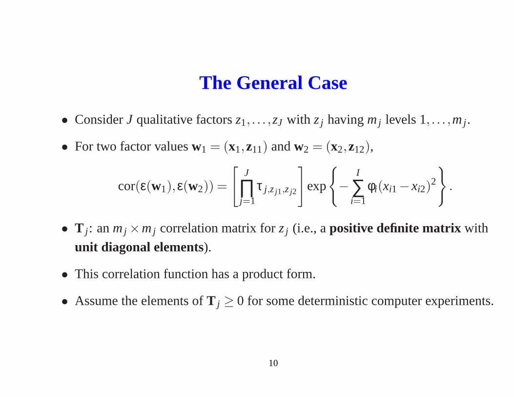
The General Case

• ConsiderJ qualitative factorsz1, . . . ,zJ with zj havingmj levels 1, . . . ,mj .

• For two factor valuesw1 = (x1,z11) andw2 = (x2,z12),

cor(ε(w1),ε(w2)) =

[J

∏j=1

τ j,zj1,zj2

]exp

{−

I

∑i=1

φi(xi1−xi2)2

}.

• T j : anmj ×mj correlation matrix forzj (i.e., apositive definite matrix with

unit diagonal elements).

• This correlation function has a product form.

• Assume the elements ofT j ≥ 0 for some deterministic computer experiments.

10

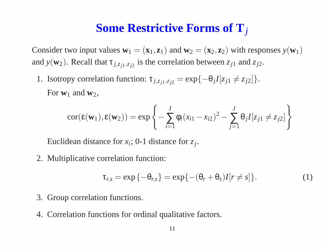
Some Restrictive Forms of Tj

Consider two input valuesw1 = (x1,z1) andw2 = (x2,z2) with responsesy(w1)

andy(w2). Recall thatτ j,zj1,zj2 is the correlation betweenzj1 andzj2.

1. Isotropy correlation function:τ j,zj1,zj2 = exp{−θ j I [zj1 6= zj2]}.

Forw1 andw2,

cor(ε(w1),ε(w2)) = exp

{−

I

∑i=1

φi(xi1−xi2)2−

J

∑j=1

θ j I [zj1 6= zj2]

}

Euclidean distance forxi ; 0-1 distance forzj .

2. Multiplicative correlation function:

τr,s = exp{−θr,s} = exp{−(θr +θs)I [r 6= s]}. (1)

3. Group correlation functions.

4. Correlation functions for ordinal qualitative factors.

11

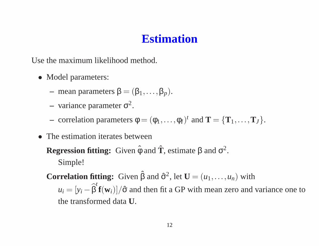
Estimation

Use the maximum likelihood method.

• Model parameters:

– mean parametersβ = (β1, . . . ,βp).

– variance parameterσ2.

– correlation parametersφ = (φ1, . . . ,φI )t andT = {T1, . . . ,TJ}.

• The estimation iterates between

Regression fitting: Given φ andT, estimateβ andσ2.

Simple!

Correlation fitting: Givenβ andσ2, let U = (u1, . . . ,un) with

ui = [yi − βtf(wi)]/σ and then fit a GP with mean zero and variance one to

the transformed dataU.

12

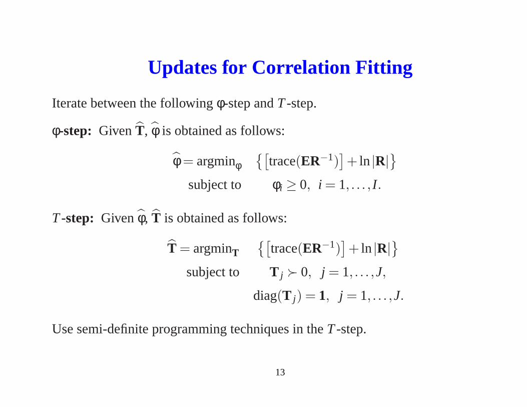
Updates for Correlation Fitting

Iterate between the followingφ-step andT-step.

φ-step: GivenT, φ is obtained as follows:

φ = argminφ{[

trace(ER−1)]+ ln |R|

}

subject to φi ≥ 0, i = 1, . . . , I .

T-step: Given φ, T is obtained as follows:

T = argminT{[

trace(ER−1)]+ ln |R|

}

subject to T j ≻ 0, j = 1, . . . ,J,

diag(T j) = 1, j = 1, . . . ,J.

Use semi-definite programming techniques in theT-step.

13

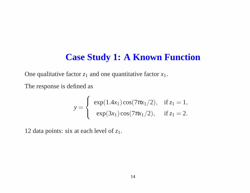
Case Study 1: A Known Function

One qualitative factorz1 and one quantitative factorx1.

The response is defined as

y =

exp(1.4x1)cos(7πx1/2), if z1 = 1,

exp(3x1)cos(7πx1/2), if z1 = 2.

12 data points: six at each level ofz1.

14

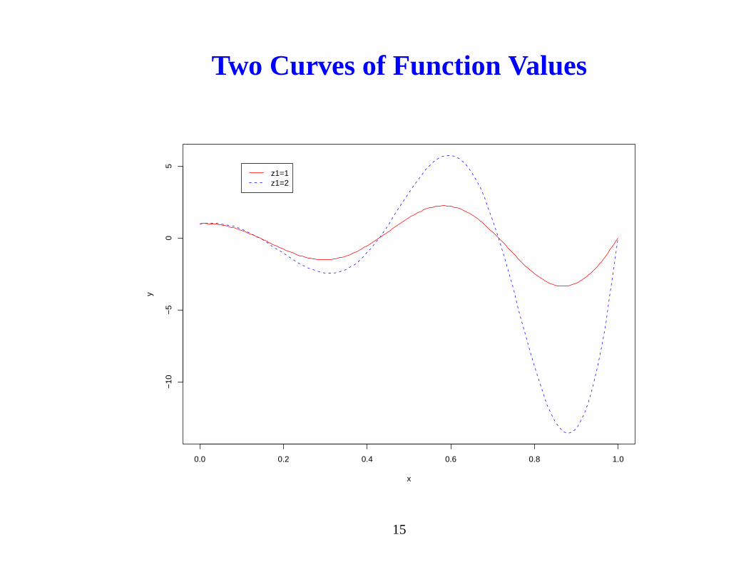
Two Curves of Function Values

0.0 0.2 0.4 0.6 0.8 1.0

−10

−5

05

x

y

z1=1z1=2

15

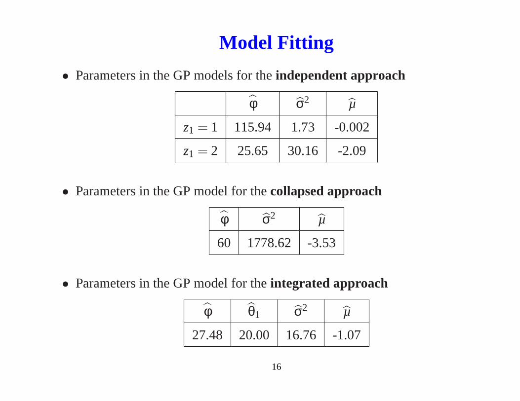
Model Fitting

• Parameters in the GP models for theindependent approach

φ σ2 µ

z1 = 1 115.94 1.73 -0.002

z1 = 2 25.65 30.16 -2.09

• Parameters in the GP model for thecollapsed approach

φ σ2 µ

60 1778.62 -3.53

• Parameters in the GP model for theintegrated approach

φ θ1 σ2 µ

27.48 20.00 16.76 -1.07

16

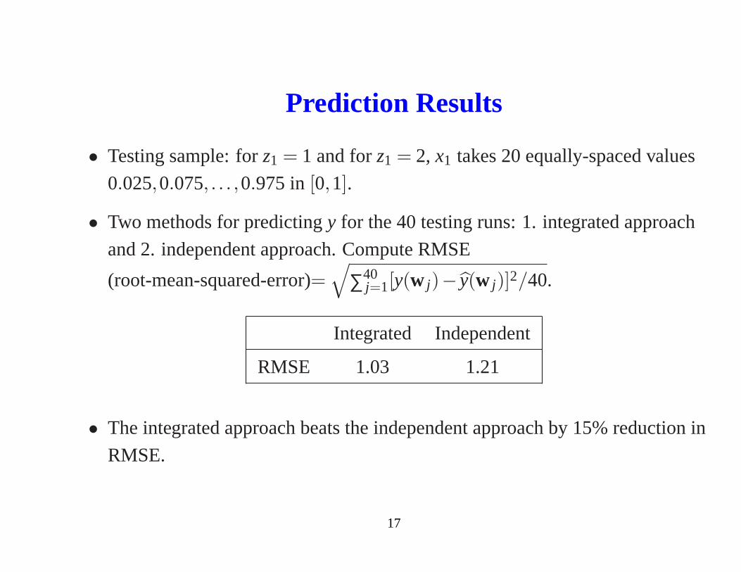
Prediction Results

• Testing sample: forz1 = 1 and forz1 = 2, x1 takes 20 equally-spaced values

0.025,0.075, . . . ,0.975 in[0,1].

• Two methods for predictingy for the 40 testing runs: 1. integrated approach

and 2. independent approach. Compute RMSE

(root-mean-squared-error)=√

∑40j=1[y(w j)− y(w j)]2/40.

Integrated Independent

RMSE 1.03 1.21

• The integrated approach beats the independent approach by 15% reduction in

RMSE.

17

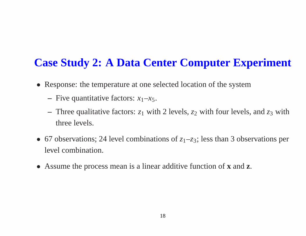
Case Study 2: A Data Center Computer Experiment

• Response: the temperature at one selected location of the system

– Five quantitative factors:x1–x5.

– Three qualitative factors:z1 with 2 levels,z2 with four levels, andz3 with

three levels.

• 67 observations; 24 level combinations ofz1–z3; less than 3 observations per

level combination.

• Assume the process mean is a linear additive function ofx andz.

18

Model Fitting

• The outer loop: iterate 20 times betweenregression fittingandcorrelation

fitting.

• The inner loop for the correlation fitting: iterate 20 times betweenφ-step and

T-step.

Parameter estimates:

• β =

(11.95,6.17,−2.77,3.05,−4.53,0.20,0.08,−0.95,−0.72,−1.73,2.66,1.27).

• Varianceσ2 = 2.85.

• φ = (7.57,1.08,1.07,7.71,3.36).

19

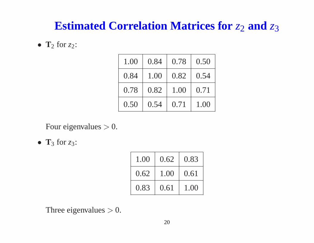
Estimated Correlation Matrices for z2 and z3

• T2 for z2:

1.00 0.84 0.78 0.50

0.84 1.00 0.82 0.54

0.78 0.82 1.00 0.71

0.50 0.54 0.71 1.00

Four eigenvalues> 0.

• T3 for z3:

1.00 0.62 0.83

0.62 1.00 0.61

0.83 0.61 1.00

Three eigenvalues> 0.

20

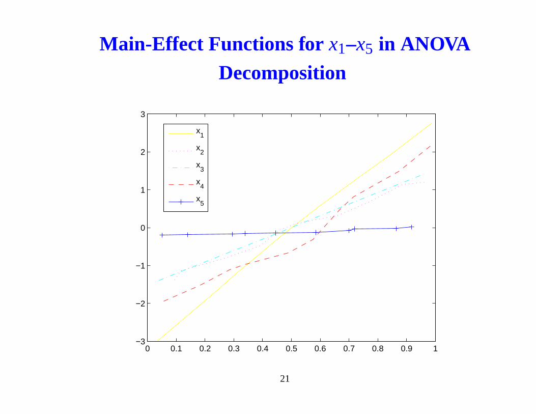
Main-Effect Functions for x1–x5 in ANOVADecomposition

0 0.1 0.2 0.3 0.4 0.5 0.6 0.7 0.8 0.9 1−3

−2

−1

0

1

2

3

x1

x2

x3

x4

x5

21

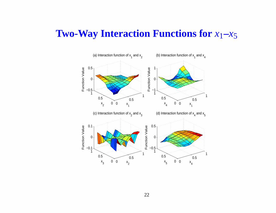
Two-Way Interaction Functions for x1–x5

00.5

1

00.5

1−0.5

0

0.5

x1

(a) Interaction function of x1 and x

2

x2

Fu

nct

ion

Va

lue

00.5

1

00.5

1−1

0

1

x1

(b) Interaction function of x1 and x

4

x4

Fu

nct

ion

Va

lue

00.5

1

00.5

1−0.1

0

0.1

x2

(c) Interaction function of x2 and x

3

x3

Fu

nct

ion

Va

lue

00.5

1

00.5

1−0.5

0

0.5

x4

(d) Interaction function of x4 and x

5

x5

Fu

nct

ion

Va

lue

22

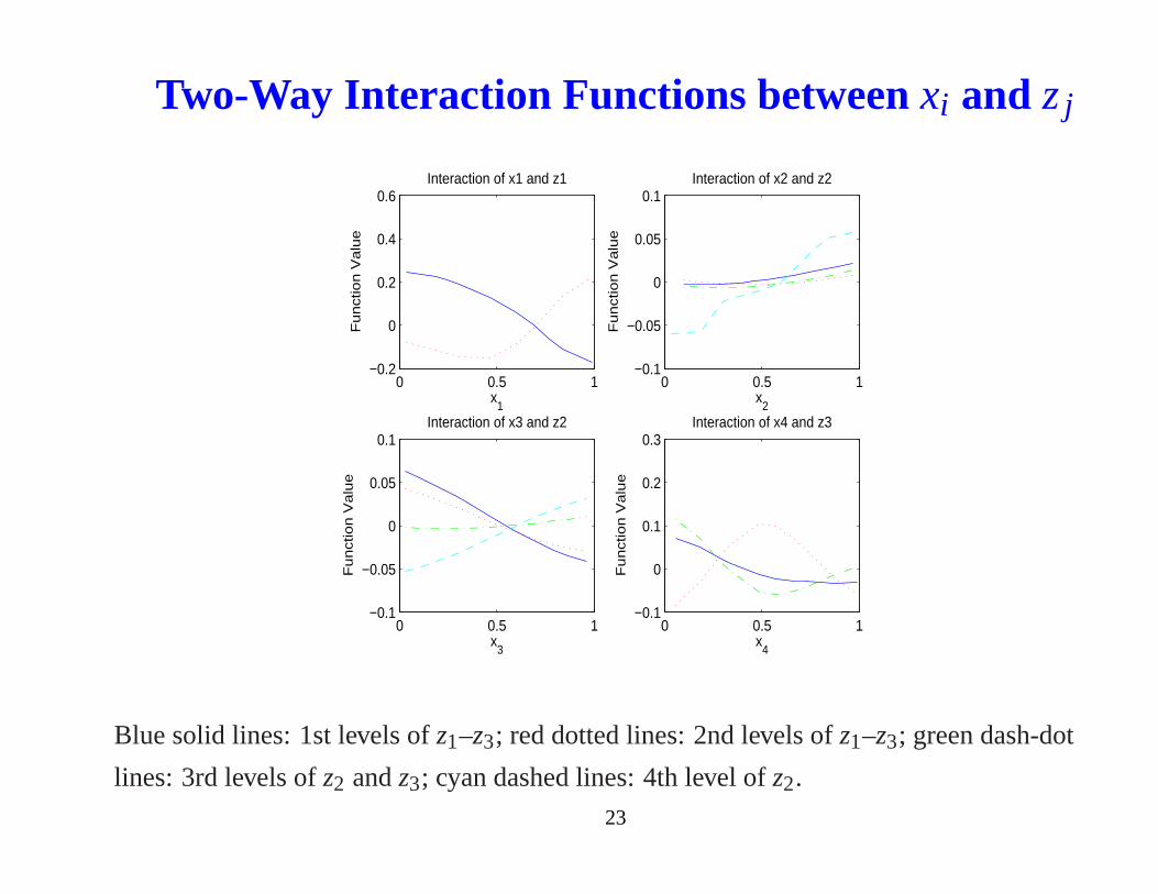
Two-Way Interaction Functions betweenxi and zj

0 0.5 1−0.2

0

0.2

0.4

0.6

x1

Fu

nct

ion

Va

lue

Interaction of x1 and z1

0 0.5 1−0.1

−0.05

0

0.05

0.1

x2

Fu

nct

ion

Va

lue

Interaction of x2 and z2

0 0.5 1−0.1

−0.05

0

0.05

0.1

x3

Fu

nct

ion

Va

lue

Interaction of x3 and z2

0 0.5 1−0.1

0

0.1

0.2

0.3

x4

Fu

nct

ion

Va

lue

Interaction of x4 and z3

Blue solid lines: 1st levels ofz1–z3; red dotted lines: 2nd levels ofz1–z3; green dash-dot

lines: 3rd levels ofz2 andz3; cyan dashed lines: 4th level ofz2.

23

A Simple Approach to Emulation for Computer

Models With Qualitative and Quantitative Factors

• Based on hypersphere decomposition of correlation matrices.

• Avoid directly solving optimization problems with positive definite

constraints.

• Can model both negative and positive cross-correlations.

• Fast to compute.

Zhou, Q., Qian, P. Z. G. and Zhou, S (2010), “A Simple Approach to Emulation for

Computer Models With Qualitative and Quantitative Factors,” tentatively accepted

by Technometrics.24

Sliced Space-Filling Designs

Proposed in Qian and Wu (2009).

Construction:

1. For the quantitative factors, generate a space-filling design by using aspecialorthogonal array.

2. Use some algebraic methods to partition the design into groups corresponding

to different level combinations of the qualitative factorssuch that the points in

each of these groups achieve uniformity in low dimensions.

Qian, P. Z. G. and Wu, C. F. J. (2009), “Sliced Space-Filling Designs,”Biometrika

96, 945-956.

25

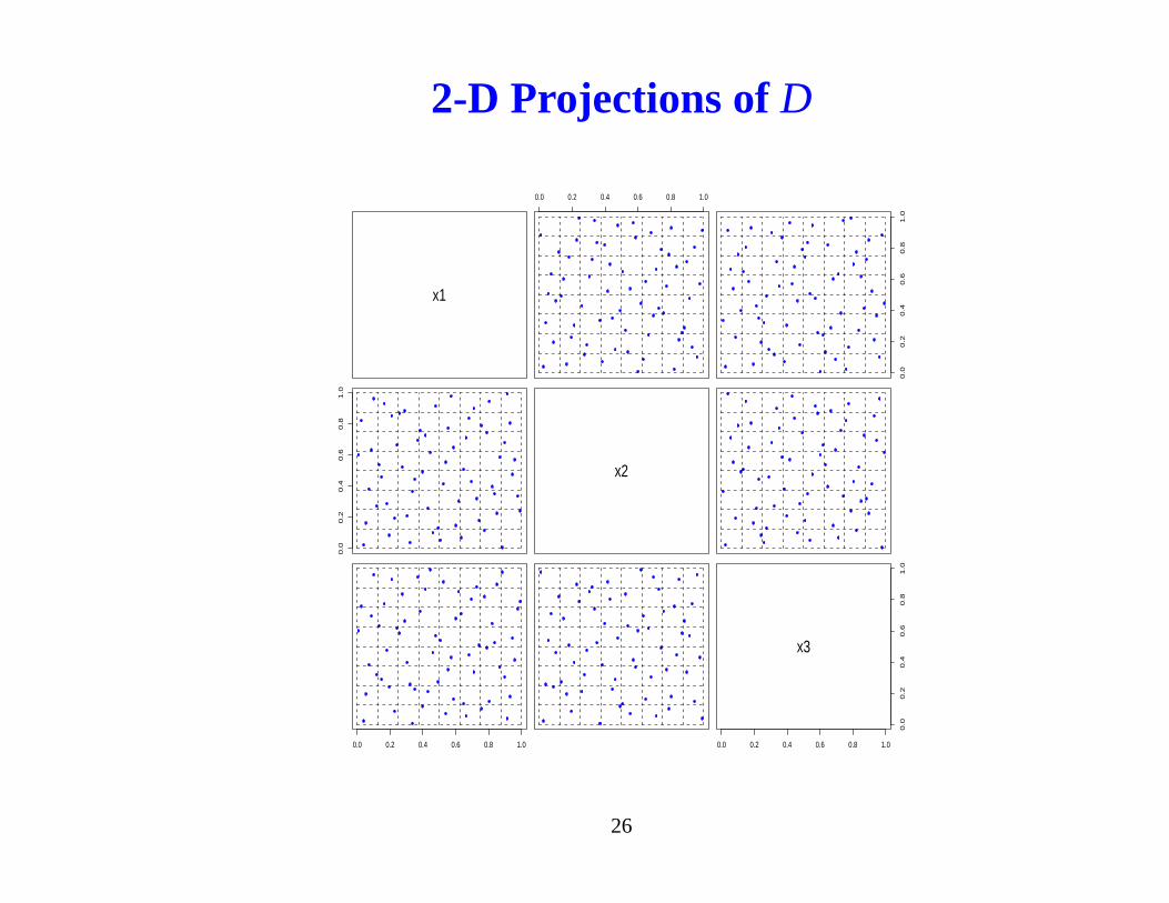
2-D Projections ofD

x1

0.0 0.2 0.4 0.6 0.8 1.0

0.0

0.2

0.4

0.6

0.8

1.0

0.0

0.2

0.4

0.6

0.8

1.0

x2

0.0 0.2 0.4 0.6 0.8 1.0 0.0 0.2 0.4 0.6 0.8 1.0

0.0

0.2

0.4

0.6

0.8

1.0

x3

26

2-D Projections ofD11

x1

0.0 0.2 0.4 0.6 0.8 1.0

0.0

0.2

0.4

0.6

0.8

1.0

0.0

0.2

0.4

0.6

0.8

1.0

x2

0.0 0.2 0.4 0.6 0.8 1.0 0.0 0.2 0.4 0.6 0.8 1.0

0.0

0.2

0.4

0.6

0.8

1.0

x3

27

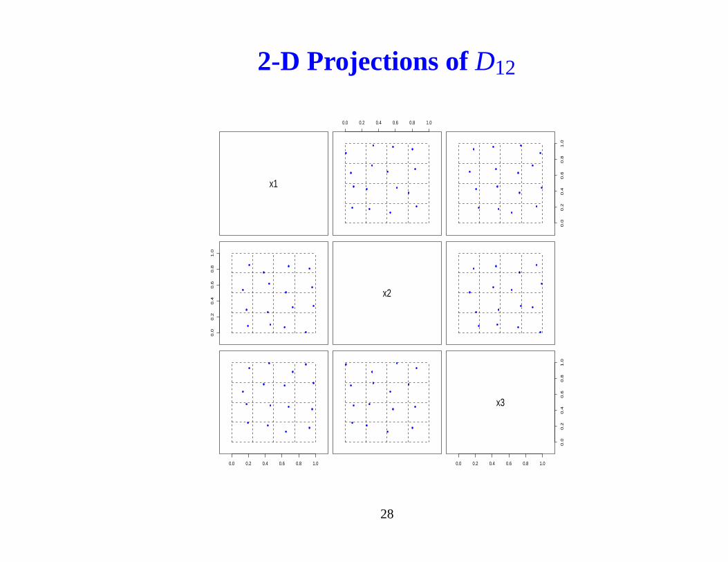
2-D Projections ofD12

x1

0.0 0.2 0.4 0.6 0.8 1.0

0.0

0.2

0.4

0.6

0.8

1.0

0.0

0.2

0.4

0.6

0.8

1.0

x2

0.0 0.2 0.4 0.6 0.8 1.0 0.0 0.2 0.4 0.6 0.8 1.0

0.0

0.2

0.4

0.6

0.8

1.0

x3

28

2-D Projections ofD21

x1

0.0 0.2 0.4 0.6 0.8 1.0

0.0

0.2

0.4

0.6

0.8

1.0

0.0

0.2

0.4

0.6

0.8

1.0

x2

0.0 0.2 0.4 0.6 0.8 1.0 0.0 0.2 0.4 0.6 0.8 1.0

0.0

0.2

0.4

0.6

0.8

1.0

x3

29

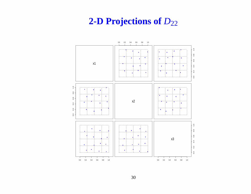
2-D Projections ofD22

x1

0.0 0.2 0.4 0.6 0.8 1.0

0.0

0.2

0.4

0.6

0.8

1.0

0.0

0.2

0.4

0.6

0.8

1.0

x2

0.0 0.2 0.4 0.6 0.8 1.0 0.0 0.2 0.4 0.6 0.8 1.0

0.0

0.2

0.4

0.6

0.8

1.0

x3

30

Thank you!

31