Deriving Small Unsatisfiable Cores withDominators

Roman Gershman Maya Koifman Ofer Strichman

Technion, Haifa, Israel. Contact: ofers@ie.technion.ac.il

Abstract. The problem of finding a small unsatisfiable core of an un-satisfiable CNF formula is addressed. The proposed algorithm, Trimmer ,iterates over each internal node d in the resolution graph that ‘consumes’a large number of clauses M (i.e. a large number of original clauses arepresent in the unsat core only for proving d) and attempts to prove themwithout the M clauses. If this is possible, it transforms the resolutiongraph into a new graph that does not have the M clauses at its core.Trimmer can be integrated into a fixpoint framework similarly to Ma-lik and Zhang’s fix-point algorithm (run till fix). We call this optiontrim till fix. Experimental evaluation on a large number of industrialCNF unsatisfiable formulas shows that trim till fix doubles, on aver-age, the number of reduced clauses in comparison to run till fix. It isalso better when used as a component in a bigger system that enforcesshort timeouts.

1 Introduction

Given an unsatisfiable CNF formula, an unsatisfiable core (UC) is any subsetof these clauses that is still unsatisfiable. The problem of finding a minimum,minimal or just a small UC has been addressed rather frequently in the lastfew years [2, 10, 16, 11, 6], partially due to its increasing importance in formalverification.

The decision problem corresponding to finding the minimum UC is a Σ2-complete problem [5] and we are not aware of an algorithms for finding it thatscales. Finding a minimal UC (any subset of clauses such that the removal ofany one of them makes the formula satisfiable), according to Papadimitriou andWolfe [12], is DP -complete1.

It is questionable whether finding a minimal UC has a practical value, how-ever, since a non-minimal UC can be smaller than a minimal one, as long as it isnot contained in it. Therefore heuristics that do not guarantee minimality, canbe both faster and better than those that guarantee minimality. The latter areuseful only when their result is compared to the core from which they started,and thus can be used, for example, after another, faster algorithm, has alreadyextracted a small core and cannot find a smaller one.1 DP is the class containing all languages that can be considered as the difference

between two languages in NP, or equivalently, the intersection of a language in NPwith a language in co-NP.

Typically UCs are needed as part of a larger system (such as an abstrac-tion/refinement loop as we will soon describe), and the influence of the size ofthe UC on the other parts of the system is only vaguely known. Hence, althoughmore computation time can lead to finding smaller cores, it is not clear whetherit is cost-effective in the overall system. This suggests once again that minimal-ity per-se is not so important in practice. Algorithms for extracting small coresshould be measured instead by their velocity : how many clauses they removefrom the initial formula per time unit, on average. They should also be mea-sured by how small they can make the core within a time limit, in comparisonwith other algorithms, and whether they can contribute to a setting in whichseveral of these algorithms are run sequentially or even in parallel. In Section 6we measure our suggested technique, called Trimmer , with these criteria.

Before we describe previous work on this problem, let us mention some ofthe typical usages of UCs. A small unsatisfiable core reflects a more precise andfocused explanation of the unsatisfiability of a given formula. In verification, it isused in several contexts, some of which are the following. Amla and McMillan [1]suggest to use UCs for a proof-based abstraction-refinement model-checking pro-cess: the UC of an unsatisfiable BMC instance contains information on the statevariables that are sufficient for proving that no bug can be found up to a givendepth; based on these state variables they build a refined abstract model andcontinue to iterate. Kroening et al. [8] use unsatisfiable cores for an iterative pro-cess of solving Presburger formulas: the UC is used for checking whether certainunder-approximating restrictions on the solution space were used in the proof ofunsatisfiability. If the answer is yes, these restrictions should be relaxed. A similarusage of UCs is by Grumberg et al. [4], in a process of under-approximation andwidening of BMC formulas corresponding to a multi-threaded process. Outsideverification, the identification of an inconsistent kernel can be important for solv-ing the inconsistency in any constraints satisfaction problem. Further, lookingbeyond the Propositional world, finding a small unsatisfiable set of constraintsis important for the efficiency of decision procedures like MathSat and CVC[15]that rely on explanations of the reason of unsatisfiability in order to prune thesearch space. The techniques we will discuss in this paper are equally relevantto such systems as they are for systems based on propositional reasoning.

Related work. Lynce and Silva [10] suggested an approach for finding a mini-mal UC, in which a new ‘clause selector’ variable csi, 1 ≤ i ≤ m, is added to eachof the m clauses of the formula (for example, the ith clause (l1 ∨ l2) is replacedwith (csi ∨ l1 ∨ l2)). The cs variable is set to true iff the clause is not selected.They then use a SAT solver that decides first on the cs variables. If all theclauses become satisfied, it backtracks to the most recent cs variable set to true.If the solver reaches a conflict and consequently backtracks to the cs variables,it means that an unsatisfiable core was found. In such a case it records the sizeof the core and continues to search for a smaller one, after adding a clause overthe cs variables that blocks the solver from repeating the same core. A similarprocess was suggested also by Oh et al. [11] (the ‘Amuse’ algorithm), although

2

they modify the backtracking mechanism so it performs a bottom-up search for aUC instead of searching for a satisfying assignment. Different decision heuristicsresult in different UCs, which are not necessarily minimal.

Huang suggests the ‘MUP’ (Minimal Unsatisfiability Prover) algorithm in [6].Rather than using m clause selector variables, he suggests to augment the clauseswith minterms over log(m + 1) variables. The augmented formula, he proves,is minimally unsatisfiable iff there are exactly m models over the y variables(because in this case every clause that is removed makes the formula satisfiable).Hence, the problem of proving that an existing set is minimal is reduced to that ofmodel-counting, which MUP performs with a variable elimination technique overBDDs. This technique can be taken one step further towards finding a minimalcore, by running it not more than m times. MUP shows better experimentalresults than run till fix (see below), but only, apparently, on hand-made andrelatively small formulas, like the pigeonhole problem. None of the benchmarksreported in [6] has more than several thousand clauses, and it is not clear howit scales to industrial problems.

A more practical approach is to find a small core without guaranteeing mini-mality, while attempting to be efficient and produce intermediate valuable resultsin case the external process does not wish to wait for the final result. Zhang andMalik [16] were the first in the verification community, as far as we know, to ad-dress this problem from a practical point of view. They suggested a simple andeffective iterative procedure for deriving a small unsatisfiable core: they extractan unsatisfiable core from an unsatisfiability proof of the formula provided by aSAT solver and then they run the SAT solver again starting from this core, whichmay result in an even smaller core. Their script run till fix repeats this pro-cess until the core is equal to a core derived in the previous iteration, or, in otherwords, until it reaches a fixpoint. The solution and its implementation seem tobe the most practical one available, and is indeed widely used. The experimentalresults that we present in Section 6 are compared against run till fix.

What is this article about? We describe a new heuristic, called Trimmer ,for finding a small UC. Trimmer takes the role of zVerify in run till fix.It can be either applied once (and generate a core smaller or equal to thatgenerated by zVerify) or as part of a fixpoint computation, in an algorithm wecall trim till fix. We will concentrate on Trimmer from hereon and return totrim till fix in the description of the experimental results.

We assume from here on that the reader is familiar with the basic inner-workings of modern DPLL-based SAT solvers, and hence describe those parts ofthe solver that our algorithm relies on only in general, abstract terms.

New conflict clauses are derived in a process called Conflict Analysis, by(conceptually) traversing backwards the conflict graph and locating the reasonfor the conflict. This process can be interpreted as a series of resolution steps[16]. The SAT solver can output a graph reflecting the resolution steps, knownas the resolution graph. The nodes of a resolution graph represent clauses, andthe single sink node of this graph represents the empty clause. Each internal

3

node has two parents, which represent the clauses from which it was resolved. Inpractice this graph can represent Hyper-resolution (a result of several resolutionsteps) and hence each node can have more than two parents. The general ideaof the Trimmer algorithm, described in detail in Section 4, is the following.Trimmer locates internal nodes in the resolution graph that dominate othernodes, called the minions (i.e., all the paths from a minion node to the sinknode go through the dominator), and checks whether they can be proved withouttheir minions. If the answer is yes, the minions can be removed, and consequentlythe size of the UC is decreased. In such a case the resolution graph has to betransformed so it reflects the new proof. This transformation is the subject ofSection 4.1. Trimmer repeats this process until no changes in the graph can bemade. Experimental results show that integrating this procedure in a fixpointscript in the style of run till fix, is better than run till fix, at least withthe relatively short timeouts we tried (30 and 60 minutes). Trimmer has theadvantage that it generates intermediate results rather fast. Hence, while inmany cases run till fix times out (i.e. it cannot finish the first iteration afterthe initial core within the time limit), Trimmer almost always finishes severaliterations by that time, even if in the long run run till fix produces smallercores.

2 Preliminaries

Resolution is a proof system for CNF formulas with one inference rule:

(A ∨ x) (B ∨ ¬x)(A ∨B)

where A,B are disjunctions of literals (possibly with 0 disjuncts, i.e. the constantfalse). The clause (A ∨ B) is the resolvent, and (A ∨ x) and (B ∨ ¬x) are theresolving clauses. The resolvent of the clauses (x) and (¬x) is the empty clause(⊥). Each application of the resolution rule is called a resolution step.

Lemma 1. A Propositional CNF formula is unsatisfiable if and only if thereexists a finite sequence of resolution steps ending with the empty clause.

A sequence of resolution steps, each one uses the result of the previous step asone of the resolving clauses of the current step, is called Hyper-resolution. Forexample, from

(x1 ∨ x2 ∨ x3)(¬x1 ∨ x4)(¬x2 ∨ x5)

we can derive (x3 ∨x4 ∨x5) by two resolution steps (first over x1, then over x2),or by one hyper-resolution step.

The hyper-resolution steps leading to the derivation of the empty clause canbe depicted in a Hyper-resolution graph (or, simply, a resolution graph). Fromhereon, we use the terms node and clause interchangeably, since every noderepresents a clause.

4

Definition 1. A Hyper-resolution graph corresponding to an unsatisfiabilityproof by resolution, is a Directed acyclic Graph G(V, E, s) with a single sinknode s ∈ V , in which the nodes represent CNF clauses: the leaf nodes (thesources) represent original clauses, the inner nodes represent clauses derived byresolution, and the sink represents the empty clause. Each node can be inferredfrom its parent nodes by some sequence of resolution steps.

Modern DPLL-based SAT solvers can output a Hyper-resolution proof ofunsatisfiability. The intermediate clauses in this proof are the conflict clausesthat were generated during the run, and that are on a path from the leafs to theempty clause.

We now generalize resolution graphs to Clause Implication Graphs:

Definition 2 (Clause Implication Graph). A Clause-Implication Graph (CIG)G(V, E, s) is a directed acyclic graph with a single sink node s ∈ V , in which thenodes represent CNF clauses, and each node is logically implied by the conjunc-tion of clauses represented by its parents.

A CIG is less restrictive than hyper-resolution graphs. They can have edges suchas

– Subsumption ((Φ), (Φ ∨ x))– Reflexive implication ((Φ), (Φ))– Resolution + Subsumption ((Φ1 ∨ x), (Φ1 ∨ Φ2 ∨ p)) together with

((Φ2 ∨ ¬x), (Φ1 ∨ Φ2 ∨ p))

where Φ1, Φ2 are disjunctions of literals, and p, x are variables. Other implicationsforbidden by hyper-resolution are also possible. Figure 1 (left) depicts an exampleof a Clause Implication Graph.

Let L denote the leaf nodes of a CIG, and assume that s represents the emptyclause. By definition of CIG, the conjunction of the L clauses is unsatisfiable,and hence there exists a corresponding resolution proof of unsatisfiability startingfrom the same nodes. Therefore, for the purpose of finding small UCs, CIGs aresufficient for the analysis. Our construction will begin from the hyper-resolutiongraph, which can be derived from the resolution trace given to us by the SATsolver, but will transform it to a CIG as the algorithm progresses.

3 Dominators

Prosser [13] introduced the notion of dominance in the context of Flowgraphanalysis (originally a term related to code analysis and compilers).

A Flowgraph G = (V, E, r) is a directed graph such that every vertex isreachable from a distinguished root vertex r ∈ V . A vertex d ∈ V dominatesv ∈ V, v 6= d, if every path from r to v includes d. d immediately dominates vif it dominates v and there is no other node on the path between them thatdominates v. We name v a minion of d. The set of minions of d is denoted byM(d). A node is called a dominator if it dominates at least one node.

5

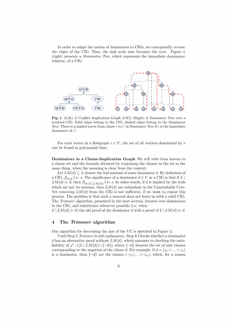
In order to adapt the notion of dominators to CIGs, we conceptually reversethe edges of the CIG. Thus, the sink node now becomes the root. Figure 1(right) presents a Dominator Tree, which represents the immediate dominancerelation, of a CIG.

(a V b) (¬b V c)

(a V c)

(¬a)

(c V d)

(¬a)

1 2 43

9

8765

14

12 13

1110

Fig. 1. (Left) A Conflict Implication Graph (CIG) (Right) A Dominator Tree over areversed CIG. Solid edges belong to the CIG, dashed edges belong to the DominatorTree. There is a dashed arrow from clause c to c′ in Dominator Tree if c is the immediatedominator of c′.

For each vertex in a flowgraph v ∈ V , the set of all vertices dominated by vcan be found in polynomial time.

Dominators in a Clause-Implication Graph We will refer from hereon toa clause set and the formula obtained by conjoining the clauses in the set as thesame thing, when the meaning is clear from the context.

Let LM(d) ⊆ L denote the leaf minions of some dominator d. By definition ofa CIG,

∧l∈L l |= s. The significance of a dominator d ∈ V in a CIG is that if L \

LM(d) |= d, then∧

l∈(L\LM(d)) l |= s. In other words, if d is implied by the leafswhich are not its minions, then LM(d) are redundant in the Unsatisfiable Core.Yet removing LM(d) from the CIG is not sufficient, if we want to repeat thisprocess. The problem is that such a removal does not leave us with a valid CIG.The Trimmer algorithm, presented in the next section, iterates over dominatorsin the CIG, and substitutes whenever possible (i.e. whenL\LM(d) |= d) the old proof of the dominator d with a proof of L\LM(d) |= d.

4 The Trimmer algorithm

Our algorithm for decreasing the size of the UC is sketched in Figure 2.Until Step 5 Trimmer is self explanatory. Step 6 Checks whether a dominator

d has an alternative proof without LM(d), which amounts to checking the satis-fiability of ϕ′ : ((L \LM(d))∪{¬d}), where {¬d} denotes the set of unit clausescorresponding to the negation of the clause d. For example, if d = (z1 ∨ . . .∨ zn)is a dominator, then {¬d} are the clauses (¬z1) . . . (¬zn), which, for a reason

6

2. Find Dominators in R

4. Select next dominator d

from dominator queue

5. Find all leaf minions of d: LM(d)

6. SAT (L\LM(d) {¬d})?

yes

7. Create Resolution Graph Rd

8. Transform Rd into proof of d: TRd

9. Remove from R:

- M(d) and their adjacent edges,

- incoming edges to d

no

End

no such d

10. Embed TRd into R

3. Create dominator queue

Dominators are

sorted according

to their number

of leaf minions,

in descending

order

L – leaves of the

current graph R

1. Input: Resolution Graph R

Output: Current

leaves L of R

Fig. 2. The Trimmer algorithm

that will soon be clear, we refer to as the assumptions. If ϕ′ is satisfiable, theattempt failed and it proceeds to the next dominator in the queue. Otherwise,relying on the equivalence

((L \ LM(d)) ∪ {¬d}) |= ⊥ ⇐⇒ L \ LM(d) |= d,

in Step 8 Trimmer transforms the hyper-resolution graph Rd into a proof of d,and builds a corresponding CIG TRd. A transformation is needed because theproof of ϕ′’s unsatisfiability, as generated by the SAT solver, is a proof of theempty clause that uses assumptions. We have to transform it into a proof of dwithout the assumptions. We discuss two different methods for performing thistransformation in Section 4.1. In step 9 Trimmer removes from R the graphelements corresponding to the old proof of d and replaces it with the new one,TRd, in step 10. That is, it removes all the minions of d together with theiradjacent edges and incoming edges to d, and embeds TRd into R instead.

Definition 3 (Graph embedding). The embedding of a graph G(V, E) in agraph G′(V ′, E′), is a graph G′′(V ′′, E′′) such that V ′′ = V ∪V ′ and E′′ = E∪E′.

After the old proof is replaced with the new one, the new graph is still aCIG, but has fewer leafs, and hence a smaller unsatisfiable core than the originalgraph.

7

4.1 Transforming the Resolution Graph

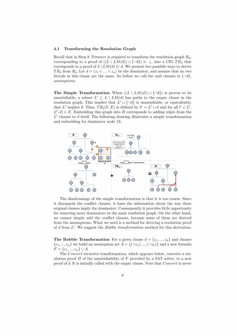
Recall that in Step 8 Trimmer is required to transform the resolution graph Rd,corresponding to a proof of ((L \ LM(d)) ∪ {¬d}) |= ⊥, into a CIG TRd thatcorresponds to a proof of L\LM(d) |= d. We present two possible ways to deriveTRd from Rd. Let d = (z1 ∨ . . .∨ zn) be the dominator, and assume that no twoliterals in this clause are the same. As before we call the unit clauses in {¬d},assumptions.

The Simple Transformation When ((L \ LM(d)) ∪ {¬d}) is proven to beunsatisfiable, a subset L′ ⊆ L \ LM(d) has paths to the empty clause in theresolution graph. This implies that L′ ∪ {¬d} is unsatisfiable, or equivalently,that L′ implies d. Thus, TRd(V, E) is defined by V = L′ ∪ d and for all l′ ∈ L′,(l′, d) ∈ E. Embedding this graph into R corresponds to adding edges from theL′ clauses to d itself. The following drawing illustrates a simple transformationand embedding for dominator node 13:

2 43

9

65

14

12 13

10

2 43

9

8765

14

12 13

1110

5 3

13

6

¬131 5 3¬132

20

21

Unit clauses with

negated literals

from the

dominator 13

An empty

clause

6

Remove proof of

13Transformation

2 43

9

65

14

12 13

10

TR13

R13R

R’

d

The disadvantage of the simple transformation is that it is too coarse. Sinceit disregards the conflict clauses, it loses the information about the way theseoriginal clauses imply the dominator. Consequently it provides little opportunityfor removing more dominators in the main resolution graph. On the other hand,we cannot simply add the conflict clauses, because some of them are derivedfrom the assumptions. What we need is a method for deriving a resolution proofof d from L′. We suggest the Bubble transformation method for this derivation.

The Bubble Transformation For a given clause d = {z1, ..., zk} and clauses{c1, ..., cn} we build an assumption set A = {(¬z1), ..., (¬zk)} and a new formulaF = {c1, ..., cn} ∪A.

The Convert recursive transformation, which appears below, converts a res-olution proof Π of the unsatisfiability of F provided by a SAT solver, to a newproof of d. It is initially called with the empty clause. Note that Convert is never

8

called with an assumption leaf (these are taken care of in lines 3 and 4), and thatthe assumption leaves do not participate in the transformed graph. The Resolvestep resolves between two transformed clauses on the same variable as the orig-inal resolution variable, if it still exists in both clauses in different polarity. Inthe end of this section we give an intuitive description of an implementation ofthis procedure, while for now we concentrate on correctness. The relevance ofthis general procedure to our case is clear: d is the dominator, A is {¬d} and{c1, . . . , cn} are the clauses of L \ LM(d).

1: procedure Convert(Node: n )2: if n is leaf then return NewNode( n )3: if left(n) = (¬zi) then return Convert(right(n))4: if right(n) = (¬zi) then return Convert(left(n))5: return NewNode( Resolve(Convert(right(n), Convert(left(n)))) )

The following drawing demonstrates a bubble transformation with Convert,where z ∈ d:

(a V z) (¬a V b)

(z V b)

( )

(¬b)

(b)

(¬z) (a V z) (¬a V b)

(z V b)

( z )

(¬b)

Transformation

Fig. 3. A bubble proof transformation, where z ∈ d

The following drawing illustrates a bubble transformation and embedding fordominator node 13:

¬131 5 3¬132

20

21

Unit clauses with

negated literals

from the

dominator 13

An empty

clause

6

Remove minions

of dominator 13Transformation

5 3

20'

21'

6

2 43

9

8765

14

12 13

1110

2 43

9

65

14

12 13

10

2 43

9

65

14

12 13

10 20'

21'

TR13

R13R

R’

d

9

Proposition 1. Let ⊥ denote the empty clause of the proof Π (the proof ofF ’s unsatisfiability). Then Convert(⊥) returns a valid resolution proof Π ′ of{c1, . . . , cn} |= d′, s.t. literals(d′) ⊆ literals(d).

Proof. We use the term proof of unsatisfiability in order to emphasize thatour proof is based on a resolution graph, not a hyper-resolution graph. Theinformation provided by the SAT solver is enough for reconstructing any ofthese graphs. In order to simplify presentation of the proof even more, we useset notation for clauses to represent their literal sets.

Let n′ = Convert(n). We will prove the proposition by induction on theresolution graph structure using the following invariant:

– n′ is well-defined– n ⊆ n′ ⊆ (n ∪ d).

Base step: if n is a leaf then n′ = n, which is well-defined and, trivially,

n ⊆ n′ ⊆ (n ∪ d)

Induction step: there are two different cases - one for lines 3 and 4, and the other- for line 5.

Lines 3 and 4: Suppose that n is an inner node that was resolved by thetwo clauses nl and nr using the resolution variable t. Let n′r = Convert(nr)and n′l = Convert(nl). If, w.l.o.g. nl = (¬zi), then, according to the algorithm:(1) n′ = n′r. Since the proof is a DAG, n′ is well-defined by the inductionhypothesis. Also, by induction: (2) nr ⊆ n′r ⊆ (nr ∪ d). It must hold that t = zi,since this is the only variable common to nl and nr. Therefore: (3) n∪{zi} = nr.Combining these expressions we get

n(3)

⊆ nr

(2)

⊆ n′r(2)

⊆ (nr ∪ d)(3)= (n ∪ {zi}) ∪ d

zi∈d= (n ∪ d)

Thereforen ⊆ n′r

(1)= n′ ⊆ (n ∪ d)

Line 5: Assuming that the invariant holds for n′r and n′l, we need to provethat a resolution step is valid on clauses n′r and n′l, i.e. that, they have oppositeliterals of at least one variable. Now, since Π was a valid proof, it must holdthat there exists a literal t so that w.l.o.g t ∈ nr and ¬t ∈ nl. Since nr ⊆ n′rand nl ⊆ n′l, it holds that t ∈ n′r and ¬t ∈ n′l. Therefore n′ can be derived byresolution between n′l and n′r on the same t, and n′ is well-defined.

We need to prove that n ⊆ n′ ⊆ (n ∪ d). Indeed,

nResolution= ((nr ∪ nl) \ {t,¬t}) Induction⊆ ((n′r ∪ n′l) \ {t,¬t}) Resolution= n′

n′ = ((n′r ∪ n′l) \ {t,¬t}) Induction⊆ (((nr ∪ d) ∪ (nl ∪ d)) \ {t,¬t})= (((nr ∪ nl) \ {t,¬t}) ∪ (d \ {t,¬t})) = (n ∪ (d \ {t,¬t})) ⊆ (n ∪ d)

10

Specially, the invariant implies that for the empty clause ⊥ :

Convert(⊥) ⊆ (⊥ ∪ d) = d

ut

It is easy to show that the resulting graph is a CIG (a resolution graph,actually).Convert can also be implemented with the following, more intuitive procedure:1: for each assumption (¬zi), 1 ≤ i ≤ n in Rd do2: Add zi to all clauses on all the paths from (¬zi) to the sink node.3: Remove the assumption (¬zi) from the graph.

It can be proven that the two procedures are equivalent up to reflexive implica-tions, although this is beyond the scope of this article.

5 Optimizations

Our tool includes the following optimizations.

1. In step 6 of the algorithm (Figure 2) rather than checking((L \ LM(d)) ∪ {¬d}), Trimmer conjoins with this formula all the conflictclauses in R that are not on any path from the minions to the sink node.This addition does not change the satisfiability of the formula, because theseclauses are logically implied by L \ LM(d). But they make the SAT solvingstage incremental[14], and hence far more efficient.

2. In step 8, if none of the assumptions participate in the proof, Trimmer takesa different route. In this case Rd, which is the proof of unsatisfiability of((L \ LM(d)) ∪ {¬d}), can also be seen as the proof of unsatisfiability ofL \ LM(d), which are a subset of the clauses in the original formula. LetL′ ⊆ L \ LM(d) be the leafs of Rd. L′ is a UC of L \ LM(d), but also ofthe original formula, and it is smaller than the smallest core known so far(because the core of the current R is L). So, Trimmer assigns R = Rd andreturns to line 2.

6 Experimental Results

The implementation of the dominator algorithm in our tool Trimmer is theSLT variant of the Lengauer-Tarjan algorithm[9] (which runs in O(|E| log |V |)time), as provided by the authors of [3] and published on their web site. We usedversion 2004.11.15 of zChaff, zVerify and run till fix for both the comparisonand the extraction of the resolution traces.

The benchmark suite is composed of 75 unsatisfiable CNF instances fromthe industrial category of the SAT competitions in the last two years, from IBMformal verification benchmarks, and BMC instances from the Sun’s PicoJava

11

benchmarks that were used in [1]. We did not include benchmarks that timed-out with both Trimmer and run till fix. The initial number of clauses rangesfrom 1, 300 to 800, 000, and the largest initial core size, which is our startingpoint, has around 160,000 clauses.

We measured two parameters: core reduction (the difference between thefinal and the initial number of clauses) and average velocity (core reductiondivided by the time spent on the reduction). We used two different timeouts -1, 800 seconds and 3, 500 seconds. Since UCs are typically used within a largersystem in which they are extracted many times, relatively short timeouts reflectwhat is practically done for best overall tuning. For such systems velocity seemsto be more relevant, assuming the process of decreasing the size of the UC isinterrupted after a while, without waiting for the smallest core possible. Thetimeouts do not include the time of the first run of the solver that extracts thefirst resolution trace, since this step is common to all tools.

The competing systems in our benchmark are:

(Z) run till fix.(A) trim till fix: running Trimmer until it terminates, then running zChaff

on the new core, then rerunning (T) starting from the new resolution graph,and so on until either a fixpoint or a timeout is reached.

(A‖Z) Running (A) and (Z) in parallel (on different machines) until the first onestops or a timeout is reached. The smallest core produced by the two pro-grams so far is the resulting core of (A‖Z). This approach can be useful if(A) and (Z) are sufficiently different, and neither one dominates the other.

(T) A single run of Trimmer.

The following table summarizes our results with time out of 3500 sec. Corereduction measures the number of clauses removed from the initial core, hencea larger number is better. An intriguing result is the superiority of (A) over(A‖Z) when it comes to clause reduction. This is because the number of clausescounted for (A‖Z) is due to the system that finishes first, which may removefewer clauses than the other system.

The comparison between (Z) and (A) reveals that trim till fix removestwice as many clauses on average as run till fix but run till fix is 50%faster. Note, however, the medians: the median of trim till fix is 5 timeslarger on core reduction and 14 times larger on velocity, which is importantin the realm of short timeouts. In other words, if we ran these benchmarkswith a shorter timeout, the results would favor trim till fix much stronger.This is also evident from Figure 5: although (Z)’s velocity is typically better, itsuffers from a large number of timeouts, which is counted as 0 velocity in ourcalculations.

System Velocity Core ReductionMed. Avg. Med. Avg.

(Z) 1.1 200.8 729 3126.8(A) 14.5 130.3 3404 6212.1(A‖Z) 14.6 239.3 3310 5985.3(T) 33.0 160.8 1464 3863.1

12

We also ran a detailed statistical analysis on the results, with the ordinarysign test – see [7] for more details. The results, referring to the differences in themedians of velocity and core reduction, are summarized in Figure 4. We see thatthere is a statistically significant difference between the competing programsboth in velocity and in core reduction, with (A) and (A‖Z) being the winners.Note that this result is consistent with our previous conclusions.

A

Z

Velocity

med = 5.76

p’ = 0.79

(med = 5.65)

( p’ = 0.79 )

med = 1.13

p’ = 0.74

(med = 0.94)

( p’ = 0.74 )

med = 1.77

p’ = 1.00

(med = 1.31)

( p’ = 1.00 )

med = 7.51

p’ = 0.79

(med = 5.42)

( p’ = 0.78 )

med = 0.00

p’ = 0.92

(med = 0.00)

( p’ = 0.92 )

A||Z

Core Reduction

med = 261

p’ = 0.82

(med = 233)

( p’ = 0.83 )

med = 200

p’ = 0.84

(med = 158)

( p’ = 0.85 )

med = 970

p’ = 0.99

(med = 922)

( p’ = 1.00)

med = 887

p’ = 0.92

(med = 811)

( p’ = 0.92 )

med = 0

p’ = 0.77

(med = 0 )

(p’ = 0.78)

A||Z

T Z

A T

Fig. 4. Results summary of the statistical analysis of the difference in median valuesof velocity and core reduction. The nodes represent the competing systems, and anedge from a to b represents 99% confidence (i.e. α = 0.01) in a’s superiority over b.med is the median of the difference of values between the parent and its child. p′ isthe estimated probability of the parent’s success (which is equal to the ratio of itssuccess). The results without parentheses correspond to a timeout of 3, 500 sec., andwithin parentheses to 1, 800 sec. (A) is the ultimate leader in core reduction, and (T)and A‖Z are the fastest.

As future work we plan to analyze acceleration, i.e. the velocity as a functionof the elapsed time: this information can lead to new strategies and help choosingthe best timeout.

References

1. N. Amla and K. McMillan. Automatic abstraction without counterexamples. InH. Garavel and J. Hatcliff, editors, TACAS’03, volume 2619 of Lect. Notes inComp. Sci., 2003.

2. R. Bruni. Approximating minimal unsatisfiable subformulae by means of adaptivecore search. Discrete Appl. Math., 130(2):85–100, 2003.

3. L. Georgiadis, R. F. Werneck, R. E. Tarjan, S. Triantafyllis, and D. I. August. Find-ing dominators in practice. In 12th Annual European Symposium on Algorithms(ESA 2004), volume 3221 of LNCS, pages 677–688, 2004.

4. O. Grumberg, F. Lerda, O. Strichman, and M. Theobald. Proof-guidedunderapproximation-widening for multi-process systems. In POPL ’05: Proceedingsof the 32nd ACM SIGPLAN-SIGACT sysposium on Principles of programminglanguages, pages 122–131. ACM Press, 2005.

13

0

10000

20000

30000

40000

50000

A_diff

0 5000 15000 25000 35000 45000 55000

Z_diff

Bivariate Fit of A_diff By Z_diff

0

500

1000

1500

2000

2500

3000

3500

4000

4500

A_Velocity

0 1000 2000 3000 4000

Z_Velocity

Bivariate Fit of A_Velocity By Z_Velocity

0

10000

20000

30000

40000

50000

A||Z_diff

0 5000 15000 25000 35000 45000 55000

Z_diff

Bivariate Fit of A||Z_diff By Z_diff

0

1000

2000

3000

4000

A||Z_Velocity

0 1000 2000 3000 4000

Z_Velocity

Bivariate Fit of A||Z_Velocity By Z_Velocity

0

5000

10000

15000

20000

25000

30000

35000

T_diff

0 5000 10000 15000 20000 25000

Z_diff

Bivariate Fit of T_diff By Z_diff

0

500

1000

1500

2000

2500

3000

3500

4000

4500

T_Velocity

0 1000 2000 3000 4000

Z_Velocity

Bivariate Fit of T_Velocity By Z_Velocity

Fig. 5. Core Reduction (top) and Velocity (bottom) of A, A‖Z and T Compared to Z

5. A. Gupta. Learning Abstractions for Model Checking. PhD thesis, Carnegie MellonUniversity, 2006. (to be published).

6. J. Huang. Mup: A minimal unsatisfiability prover. In Proc. of the 10th Asia andSouth Pacific Design Automation Conference (ASP-DAC), pages 432–437, 2005.

7. M. Koifman. An approach to extracting a small unsatisfiable core. M.sc. thesis,Technion - I.I.T., Israel, Haifa, (to be published) 2006.

8. D. Kroening, J. Ouaknine, S. Seshia, and O. Strichman. Abstraction-based satis-fiability solving of Presburger arithmetic. In R. Alur and D. Peled, editors, Proc.16th Intl. Conference on Computer Aided Verification (CAV’04), number 3114 inLect. Notes in Comp. Sci., pages 308–320, Boston, MA, July 2004. Springer-Verlag.

9. T. Lengauer and R. E. Tarjan. A fast algorithm for finding dominators in a flow-graph. ACM Trans. Program. Lang. Syst., 1(1):121–141, 1979.

10. I. Lynce and J. Marques-Silva. On computing minimum unsatisfiable cores. InProceedings of the International Symposium on Theory and Applications of Satis-fiability Testing, pages 305–310, 2004.

11. Y. Oh, M. N. Mneimneh, Z. S. Andraus, K. A. Sakallah, and I. L. Markov. Amuse:a minimally-unsatisfiable subformula extractor. In DAC ’04, pages 518–523, 2004.

12. C. H. Papadimitriou and D. Wolfe. The complexity of facets resolved. J. Comput.Syst. Sci., 37(1):2–13, 1988.

13. R. Prosser. Applications of boolean matrices to the analysis of flow diagrams. InProceedings of the Eastern Joint Computer Conference, pages 133–138, 1959.

14. O. Shtrichman. Prunning techniques for the SAT-based bounded model check-ing problem. In proc. of the 11th Conference on Correct Hardware Design andVerification Methods (CHARME’01), Edinburgh, Sept. 2001.

15. A. Stump, C. Barrett, and D. Dill. CVC: a cooperating validity checker. In Proc.14th Intl. Conference on Computer Aided Verification (CAV’02), 2002.

16. L. Zhang and S. Malik. Extracting small unsatisfiable cores from unsatisfiableboolean formula. In Theory and Applications of Satisfiability Testing, 2003.

14