Derivation of an Applied Nonlinear Schroedinger...

Unclassified Unlimited Release

SANDIA REPORTSAND2015-0053Unlimited ReleasePrinted January 2015

Derivation of an Applied NonlinearSchrodinger Equation

Todd A. Pitts, Mark R. Laine, Jens Schwarz,Patrick K. Rambo and David B. Karelitz

Prepared bySandia National LaboratoriesAlbuquerque, New Mexico 87185 and Livermore, California 94550

Sandia National Laboratories is a multi-program laboratory managed and operated by Sandia Corporation,a wholly owned subsidiary of Lockheed Martin Corporation, for the U.S. Department of Energy’sNational Nuclear Security Administration under contract DE-AC04-94AL85000.

Approved for public release; further dissemination unlimited.



Issued by Sandia National Laboratories, operated for the United States Department of Energyby Sandia Corporation.

NOTICE: This report was prepared as an account of work sponsored by an agency of the UnitedStates Government. Neither the United States Government, nor any agency thereof, nor anyof their employees, nor any of their contractors, subcontractors, or their employees, make anywarranty, express or implied, or assume any legal liability or responsibility for the accuracy,completeness, or usefulness of any information, apparatus, product, or process disclosed, or rep-resent that its use would not infringe privately owned rights. Reference herein to any specificcommercial product, process, or service by trade name, trademark, manufacturer, or otherwise,does not necessarily constitute or imply its endorsement, recommendation, or favoring by theUnited States Government, any agency thereof, or any of their contractors or subcontractors.The views and opinions expressed herein do not necessarily state or reflect those of the UnitedStates Government, any agency thereof, or any of their contractors.

Printed in the United States of America. This report has been reproduced directly from the bestavailable copy.

Available to DOE and DOE contractors from

U.S. Department of EnergyOffice of Scientific and Technical InformationP.O. Box 62Oak Ridge, TN 37831

Telephone: (865) 576-8401Facsimile: (865) 576-5728E-Mail: [email protected] ordering: http://www.osti.gov/bridge

Available to the public from

U.S. Department of CommerceNational Technical Information Service5285 Port Royal RdSpringfield, VA 22161

Telephone: (800) 553-6847Facsimile: (703) 605-6900E-Mail: [email protected] ordering: http://www.ntis.gov/help/ordermethods.asp?loc=7-4-0#online

DE

PA

RT

MENT OF EN

ER

GY

• • UN

IT

ED

STATES OFA

M

ER

IC

A

2 Unclassified Unlimited Release


SAND2015-0053Unlimited Release

Printed January 2015

Derivation of an Applied Nonlinear Schrodinger

Equation

Todd A. Pitts∗ Mark R. Laine Jens Schwarz Patrick K. RamboDavid B. Karelitz

∗Sandia National Laboratories, P.O. Box 5800, MS-0980, Albuquerque, NM 87185

Abstract

We derive from first principles a mathematical physics model useful for understanding nonlinearoptical propagation (including filamentation). All assumptions necessary for the development are clearlyexplained. We include the Kerr effect, Raman scattering, and ionization (as well as linear and nonlinearshock, diffraction and dispersion). We explain the phenomenological sub-models and each assumptionrequired to arrive at a complete and consistent theoretical description. The development includes therelationship between shock and ionization and demonstrates why inclusion of Drude model impedanceeffects alters the nature of the shock operator.

Unclassified Unlimited Release 3

Contents

1 Introduction . . . . . . . . . . . . . . . . . . . . . . . . . . . . . . . . . . . . . . . . . . . . . . . . . . . . . . . . . . . . . . . . . . . . . . . . . . . . . . . . . . . . . 72 Mathematical Physics Development . . . . . . . . . . . . . . . . . . . . . . . . . . . . . . . . . . . . . . . . . . . . . . . . . . . . . . . . . . . . . . 8

2.1 Propagation Model . . . . . . . . . . . . . . . . . . . . . . . . . . . . . . . . . . . . . . . . . . . . . . . . . . . . . . . . . . . . . 82.2 Nonlinear Material Model . . . . . . . . . . . . . . . . . . . . . . . . . . . . . . . . . . . . . . . . . . . . . . . . . . . . . . . . 14

3 Summary of Physical Model . . . . . . . . . . . . . . . . . . . . . . . . . . . . . . . . . . . . . . . . . . . . . . . . . . . . . . . . . . . . . . . . . . . . . . 21

Appendix

A Symbols. . . . . . . . . . . . . . . . . . . . . . . . . . . . . . . . . . . . . . . . . . . . . . . . . . . . . . . . . . . . . . . . . . . . . . . . . . . . . . . . . . . . . . . . . . 23

5

1 Introduction

Mathematical modeling of intense optical pulse propagation physics via nonlinear Schrodinger equations findsapplication in a very large number of fields. Optical parametric amplifiers and oscillators [23, 11], secondharmonic generation [19] and third harmonic generation [36], Raman scattering [37], optical bistability[21], and solitons [24, 25, 33], are but a few of the physical phenomena with broad practical application.The scientific and engineering communities have significant efforts in the numerical modeling [29, 12, 1, 2,13] of these phenomena for both commercial and scientific research purposes. In this report we derive ageneral nonlinear Schrodinger equation from first principles paying particular attention to the physical andmathematical assumptions necessary to arrive at each step. A variety of models and unit systems are used inthe literature to describe various subsets of known physical effects (see Brabec [9], Couairon [13], or Zozulya[40]). Here we bring the physical phenomena of interest under the same framework using a single commonnotation and unit system.

The development proceeds as follows. We derive the physics model beginning with Maxwell’s equationsin section 2. The nonlinear and linear portions of a basic propagation model are introduced in section 2.1.We also discuss removal of the optical fast phase component resulting in an envelope propagation modeland introduce a retarded coordinate system traveling at the pulse group velocity in order to simplify thedescription. Section 2.2 explicitly details specific nonlinear material models for the physics of interest. Theinstantaneous or Kerr material response is described in section 2.2.1. Section 2.2.2 describes delayed Kerror Raman scattering and shows how and why it is generally combined with the instantaneous Kerr responsein mathematical models. Ionization is discussed in section 2.2.3. The description of ionization covers multi-photon and tunneling regimes as well as recombination and saturation effects. It also includes both a simpleand a Drude (ion-molecule collision) ionization current model. The latter leading to the concept of ionizationcurrent impedance. Of particular note is the development of the shock operator when including Drude model(collision) effects in the description of ionization in section 2.2.3. Inclusion of these effects, in the mannershown in our paper, leads to a difference in the form of the operator from some reports in the literature (see[13] for example). The entire mathematical model is summarized concisely in section 3. Appendix A givesan exhaustive description of all symbols used in the text.

7

2 Mathematical Physics Development

In this section we lay out the basis of the mathematical physics model. Beginning with the fundamentalgoverning equations for electromagnetics, we develop a parabolic wave equation together with a set ofnonlinear operators. The model accounts for diffraction, linear material dispersion, self-focusing (Kerr effect),ionization (energy loss and defocusing), and Raman interaction. We retain terms accounting for space-timefocusing (see Zozulya [39]) and shock (see Brabec [8]). For clarity in the developments that follow we usebold-face to indicate vector variables, plain type for scalar quantities, and eventually a calligraphic font forvariables describing envelope quantities (see Eqs. (29) and (30)). In general these variables are functions oftime and space. The temporal Fourier transform of a quantity is a function of frequency and space and isindicated via a small caret or hat over the variable (see Eqs. (17a) and (17b)).

Classical free-space electromagnetic phenomena are governed by Maxwell’s equations

∇×E = −∂tB Faraday’s Law (1)∇×H = J + ∂tD Ampere’s Law (2)∇ ·D = ρ Electric Gauss’ Law (3)∇ ·B = 0 Magnetic Gauss’ Law (4)

where

E = Electric field strength (volts/meter)H = Magnetic field strength (amperes/meter)D = Electric flux density (coulombs/square meter)B = Magnetic flux density (webers/square meter)J = Current density (amperes/square meter)ρ = Electric charge density (coulombs/cubic meter)

are functions of time and space. In order to obtain a solution for a particular problem we need additionalequations relating the field quantities. These constitutive expressions specify the relationships between fieldquantities that are functions of the specific material interacting with the fields. In free space we have

D = εoE (5)B = µoH, (6)

where the free-space permittivity and permeability are

εo = 8.854× 10−12 F/m (7)

µo = 4π × 10−7 H/m. (8)

2.1 Propagation Model

If the field interacts with a physical material, we must introduce descriptive models of the relationshipsbetween electric field and electric flux density and between magnetic field and magnetic flux density. Fora dielectric material we may modify Eq. (5) by modeling the polarization response of the material. Thefield quantity D is often given in units of Coulombs per square meter. However, it may be more intuitivelyconsidered in units of charge separation per unit volume or Coulomb meters per cubic meter. We may adda term (also with units of charge separation per unit volume) representing the total polarization response ofthe material

D = εoE + P = εoE + Pl + Pnl (9)

where we have written the total polarization P as a sum of linear and nonlinear responses Pl and Pnl

respectively. We model the linear portion of the response as directly proportional to the electric field

8

amplitude. The linear susceptibility for a particular material tells us how much charge separation per unitvolume is generated through material polarization for a given electric field strength. The linear portion ofthe model is generally given in the frequency domain as

Dl(ω) = εoE(ω) + εoχ(1)(ω)E(ω) = εoεr(ω)E(ω) (10)

where the linear susceptibility χ(1)(ω) and relative permittivity εr(ω) are functions of frequency, representinglinear dispersion. In the time domain, this relationship is expressed via convolution as

D(t) =∫ t

−∞ε(t− t′)E(t′)dt′ + Pnl, (11)

where total linear permittivity is given as ε(t) = εoεr(t).

Eqs. (1) and (2) yield the most general form of the wave equation for nonlinear optics

∇×∇×E +1εoc2

∂2tD(t) +

1εoc2

∂tJ = 0 (12)

where µ0 = 1/εoc2. For our purposes, the electric flux density is then sufficiently described as in Eq. (11).

For any vector A [16]∇×∇×A = ∇(∇ ·A)−∇2A, (13)

which may be used in Eq. (12) to arrive at

−∇2E +1εoc2

∂2tD(t) +

1εoc2

∂tJ = 0, (14)

provided ∇(∇ · E) ≈ 0. For linear, isotropic source-free media, Eq. (3) would allow us to conclude that thedivergence of the electric field is identically zero. However, for nonlinear optics this is never really the casedue to the more general relationship between the electric field and the electric flux density given in Eq. (11)[7]. The assumption is, however, valid in circumstances where the fields are primarily transverse (it breaksdown for high numerical apertures). In the remainder of this paper we take Eq. (14), often referred to asthe paraxial approximation, as sufficient for our purposes. Using Eqs. (11) through (14) we may write

∇2E− 1c2∂2t

∫ t

−∞εr(t− t′)E(t′)dt′ =

1εoc2

(∂2tPnl + ∂tJ) (15)

which forms the basis for development of many practical nonlinear propagation models.

If ionization is not included (current J is zero in Eq. (15)), we have Brabec’s [9] initial equation. If theresponse of the material and the electric field are transverse and the polarization may be considered linear,we have the scalar equation

∇2E − 1c2∂2t

∫ t

−∞εr(t− t′)E(t′)dt′ =

1εoc2

∂2tNpE. (16)

For convenience in Eq. (16) we have combined the polarization and current terms. The difference in theorder of the derivatives operating on each means that we express the combined nonlinear term Np as the sumof nonlinear polarization and the integral of current density. Although we do not explicitly state it here, thenonlinear operator is understood to be a function of the electric field. In order to create a tractable modelwe make a few more assumptions that allow a physical description of how the pulse envelope (rather thanthe instantaneous electric field amplitude) propagates.

In the subsequent development we make use of the Fourier transform. The many different representationsof the transform differ by scale factors and conjugation. In order to provide clarity in what follows we define

9

the transform explicitly as

f(t) =1

2π

∫ ∞−∞

dω f(ω)e−iωt (Synthesis) (17a)

f(ω) =∫ ∞−∞

dt f(t)eiωt (Analysis) (17b)

It is important to understand the nature of the approximations made before developing the numericalmodel. It is useful in the following to write the Laplacian as the sum of longitudinal and transverse com-ponents. We also make use of the Fourier transforms defined in Eqs. (17a) and (17b) to move the temporaloperators to the frequency domain, giving

(∂2z +∇2

⊥)E + k2(ω)E = − ω2

εoc2Np, (18)

where

k(ω) ≡ω√ε(ω)c

, (19)

andNp = FNpE. (20)

Our interest in this paper is the propagation of optical pulses. As such we introduce the concept of anelectromagnetic pulse per Born and Wolf[6].

E(r, t) = <∫ ∞−∞

aω(r)e−i[ωt−gω(r)] dω

(21)

where < is the real part of operator, describes an optical pulse or wave group if the phase function gω(r)can be meaningfully approximated by a linear function of frequency ω over the range where amplitude aω(r)differs appreciably from zero. When this is the case, the concept of a pulse can be used to model thepropagation of an electromagnetic disturbance which retains some sense of limited support (the region overwhich it is non-zero) in space and time as it moves. This may be seen via the Fourier Shift Theorem (seeBracewell [10]) which states that translation of a function in the spatial or temporal domain corresponds toa linear phase shift in its Fourier transformed distribution [10]. Eq. (21) describes the instantaneous electricfield as a function of space and time. In what follows, we use the typical convention of discussing the complexfield (without taking the real part of the right hand side in Eq. (21)). Ultimately we develop propagationequations in terms of a complex pulse envelope in order to make the numerical modeling problem feasible.

As we observe the optical disturbance propagate in a dispersive material the pulse description given inEq. (21) gives rise to two concepts of velocity. Phase velocity describes the motion of the surfaces of constantphase in the wave group, while group velocity describes the rate at which surfaces of constant amplitudetravel. We may also view the group velocity as a description of how fast the wave envelope travels. In anon-dispersive medium the group and phase velocities are the same. Phase velocity and group velocity aregiven respectively as

vp =ω

kand vg =

dω

dk=(dk

dω

)−1

≡ 1k′, (22)

where the final definition may be understood with the help of Eq. (41). We later transform our propagationphysics into a coordinate system that moves at the group velocity so that our numerical grid moves alongwith the pulse (eliminating the need for a grid covering all of the space between source and destination).

Having established that the pulse must have effectively finite support in the temporal frequency domainwe may define a center frequency. The principal purpose of the center frequency definition is to allow us

10

to later “factor out” or “eliminate” a fast phase component of our description thus facilitating a discretenumerical model with lower sampling requirements. We take Brabec’s[9] definition given as

ωo ≡∫∞odω ω|E(ω)|2∫∞

odω |E(ω)|2

, (23)

Naturally, during nonlinear propagation the center frequency per Eq. (23) will change as the pulse spec-trum is altered. Hence, ωo really represents the center frequency of the pulse before the onset of nonlinearpropagation.

We now transform to a coordinate system traveling at the group velocity of the pulse (t, z) → (τ, ζ),where

τ = t− k′z, ζ = z. (24)

From the chain rule we obtain∂t = ∂τ , ∂z = ∂ζ − k′∂τ (25)

The temporal frequency domain representations of the operators in Eq. (25) are

∂t = −iω, ∂z = ∂ζ + ik′ω. (26)

We now express Eq. (18) in the pulse reference frame via operator substitution as

[(∂ζ + ik′ω)2 +∇2⊥]E + k2(ω)E = − ω2

εoc2Np, (27)

where E ≡ E(r, τ, ζ). Eq. (27) is a carrier-resolved description in the pulse reference frame expressed in thetemporal frequency domain. We refer to the center frequency described in Eq. (23) as the carrier. In orderto facilitate subsequent development we expand one of the operators in Eq. (27) to obtain

∂2ζ E + 2ik′ω∂ζE = −∇2

⊥E − [k2(ω)− (k′ω)2]E − ω2

εoc2Np. (28)

Ultimately our model will be written in terms of envelope variables in order to create a computationallyviable framework. We now introduce the envelope models. For the laboratory fixed frame we write

E(r, t, z) = <E(r, t, z) exp(−iωot+ ikz). (29)

From Eq. (29) via Eqs. (24) we have

E(r, τ, ζ) = <E(r, τ, ζ) exp(−iωoτ + i(k − k′ωo)ζ), (30)

for the moving pulse frame. In Eqs. (29) and (30) the quantity E represents the instantaneous scalar electricfield amplitude while E is the envelope of the electric field.

Envelope models are useful when two distinct temporal scales exist in a propagation problem. Theyallow us to separate a fast scale (oscillation of the instantaneous electric field amplitude) from a slow scale(overall shape of the optical pulse). The envelope is complex, allowing phase variation (deviation from thefast phase) over the duration of the pulse to be described. The complete electric field can be reconstructedfrom this envelope easily as the real part of the product of the envelope and the fast phase component. Inorder to arrive at a propagation relationship expressed in terms of only envelope variables we will need tosubstitute each envelope term into Eq. (28) accounting for the effect of the first and second order derivativeswith respect to ζ on the envelope expression. Using Eq. (30) we obtain the following general relationship forthe nth derivative of the envelope with respect to ζ,

∂nζ E = exp(−iωoτ + i(k − k′ωo)ζ)[∂ζ + i(k − k′ωo)]nE , (31)

with Fourier transform in the temporal variable τ

∂nζ E = exp(i(k − k′ωo)ζ)[∂ζ + i(k − k′ωo)]nE , (32)

11

where E is a function of ω − ωo (see Bracewell [10]). Assuming a similar envelope model for the nonlinearpolarization term (see [12], page 30), we may use Eq. (32) and Eq. (28) to obtain (after canceling theubiquitous complex exponential term)

∂2ζ E + 2iκ(ω)∂ζ E = −∇2

⊥E − (k2(ω)− κ2(ω))E − ω2

c2εoNp (33)

where κ(ω) = k + k′(ω − ωo), andNp = FNpE (34)

Note that κ(ω) is really the sum of the first two terms in the Taylor series expansion of k(ω). In writingEq. (33) using variable envelopes we have presumed that it is possible to write the nonlinear operators inenvelope form. In section 2.2 we show that this is possible.

We make an essential approximation that produces an initial value problem from the second order partialdifferential Eq. (33) by requiring

|∂2ζ E | 2κ(ω)|∂ζ E |. (35)

Eq. (35) indicates that the magnitude of the change in ∂ζ E is small when compared with the actual magnitudeof ∂ζ E scaled by κ(ω) (which is approximately inversely proportional to the spatial wavelength). In otherwords, the magnitude and phase of the pulse envelope evolve slowly with respect to the motion of the pulsein the ζ-direction. In order to maintain slow evolution of the pulse as we move in the principle directionof propagation, we cannot allow angular spectrum components with large angles. This implies a paraxialmodel (similar to the assumption used to obtain Eq. (14)).

Using the approximation in Eq. (35) to simplify Eq. (33) yields

∂ζ E =i

2κ(ω)∇2⊥E + i

k2(ω)− κ2(ω)2κ(ω)

E + iω2

2κ(ω)c2εoNp. (36)

Eq. (36) is one-way, meaning that it presumes reflected waves are insignificant (see Feit and Fleck [17]).Also, we have placed restrictions only on the evolution of the pulse in the ζ-direction, meaning that steepchanges in the envelope along the temporal axis are allowed.

The frequency content of the pulse envelope is naturally much lower than that of the pulse itself (meaning∆ω ωo). Specifically, factoring out the carrier has left a pulse envelope description centered about thecarrier frequency (the carrier frequency is at the origin of a spectral plot of the envelope). The envelopefrequencies are really differences from the carrier and the frequency axis relationship between the envelopeand the pulse is Ω = ω − ωo.

The first term on the right-hand side of Eq. (36) operates on transverse coordinates only and representsdiffraction. The last term represents the nonlinear material response. The center term is our dispersionmodel. It represents the linear material response. We know that κ(ω) is the sum of the first two terms in theTaylor series expansion of k(ω). The difference between κ(ω) and k(ω) is comprised of higher order (secondand above) Taylor series terms. Thus we know that the expression

k2(ω)− κ2(ω)2κ(ω)

, (37)

describes the dispersion of the envelope under our model. The ratio of angular frequency to wavenumbergives the corresponding phase velocity. We know that in our moving coordinate system the phase velocities ofeach frequency must be adjusted by the velocity of the numerical grid (which is by design the group velocityof the pulse). Frequencies traveling at the group velocity should have phase velocities of zero. Those travelingfaster should have positive phase velocities. Those traveling slower must have negative phase velocities sothat they can move backward on our computational grid. With a little algebra we may approximate thedispersion relationship in Eq. (37) as

k2(ω)− κ2(ω)2κ(ω)

= [k(ω)− κ(ω)](

1 +k(ω)− κ(ω)

2κ(ω)

)≈ k(ω)− κ(ω), (38)

12

where the neglected terms are necessarily fourth order in Ω. Using Eq. (38) in Eq. (36) gives

∂ζ E =i

2κ(ω)∇2⊥E + i(k(ω)− κ(ω))E + i

ω2

2κ(ω)c2εoNp. (39)

The dispersion relationship in Eqs. (38) and (39) may also be expressed as a Taylor series expansion

D(Ω) ≡ k(ω)− κ(ω) =∞∑m=2

k(m)

m!Ωm, (40)

where the wavenumber

k(m) =∂mk(ω)∂ωm

∣∣∣∣ω=ωo

. (41)

The sum in Eq. (40) begins at m = 2 because κ(ω) subtracts off the first two terms of the series. Oftenthe first three dispersion coefficients defined by Eq. (41) are written as k′, k′′, and k′′′ respectively and weadhere to that convention in our development.

We now transform Eq. (39) back into the time domain. We can express everything in terms of the slowfrequency variable Ω = ω − ωo. Remember that

∂τ → −iΩ or i∂τ → Ω (42)

so that

ω = ωo + Ω→ ωo

(1 +

i

ωo∂τ

). (43)

Also,

κ(ω) = k + k′Ω→ k

(1 + i

k′

k∂τ

)≈ k

(1 +

i

ωo∂τ

), (44)

where the final approximation assumes the group velocity is nearly equal to the phase velocity. If we identifythe shock operators

T ≡(

1 +i

ωo∂τ

)and S ≡

(1 + i

k′

k∂τ

), (45)

we then have

∂ζE =i

2kS−1∇2

⊥E + iD(i∂τ )E +iωo

2nocεoS−1T 2NpE , (46)

where we have used ck = noωo. Using Eq. (44) we simplify the propagation description to

∂ζE ≈i

2kT−1∇2

⊥E + iD(i∂τ )E +iωo

2nocεoTNpE . (47)

In order to obtain nonlinear terms with forms familiar from the literature it is convenient to define

N ≡ iko2noεo

Np (48)

and write

∂ζE ≈i

2kT−1∇2

⊥E + iD(i∂τ )E + TNE (49)

Often only the first two terms (m = 2, 3) in the summation D(i∂τ ) are retained. These are called groupvelocity dispersion and third order dispersion respectively.

13

2.2 Nonlinear Material Model

In this section we outline the physics behind the nonlinear portion of the mathematical model. Section 2.2.1discusses the nearly instantaneous refractive index perturbation introduced into the medium by the presenceof the strong electric field associated with a high intensity optical disturbance (referred to as the Kerr effect).We derive an expression for the nonlinear refractive index (the constant of proportionality relating the cubeof the field value to the nonlinear polarization of the medium). This nonlinear polarization directly affectsthe propagation of the optical pulse via wave front delay caused by the increase in refractive index or decreasein wavespeed in high-intensity regions of the pulse and is primarily responsible for self-focusing. Section 2.2.2describes stimulated Raman scattering. This effect is also third order in field value. It is a delayed ratherthan an instantaneous effect and is represented by a convolution operator.

2.2.1 Instantaneous Kerr Effect

The Kerr effect represents nonlinear electronic polarization that takes place nearly instantaneously. Cen-trosymmetry (crystallographic or molecular) refers to a distribution containing an inversion center as one ofits symmetry elements. For every point (x, y, z) in the distribution (unit cell for solids and molecule for liq-uids and gasses) there is an indistinguishable location (−x,−y,−z). The absence of this type of symmetry isrequired in order to display properties such as the piezoelectric effect, the Pockels effect, optical rectification,etc. Centrosymmetric materials have an electronic polarization response that can be described via a Taylorseries expansion in odd powers.

P = εoχ(1)E + εoχ

(3)(E ·E)E + · · · (50)

The first order term gives rise to the concept of refractive index. Its frequency dependence introduces theconcept of dispersion and results in the convolution integral in Eq. (11) and the Taylor expansion of time-derivatives in Eqs. (46) and (49). For the nonlinear polarization operator expression in a centrosymmetricmaterial we have

NpE = εoχ(3)(E ·E)E. (51)

Using the envelope model (either lab or pulse frame written as the average of complex conjugates) we maywrite

E(r, t, z) =12

(E(r, t, z) exp(−iωot+ ikz) + c.c.), (52)

where c.c. refers to the complex conjugate of the first term. Eqs. (52) and (51) give

E3(r, t, z) =18

(E3(r, t, z) exp(−i3ωot+ i3kz)

+ 3|E|2E exp(−iωot+ ikz) + c.c.). (53)

Each term of an envelope model is written as the product of a slowly varying term and a fast phase term(complex exponential) with common frequency ωo (see Eqs (29) and (30)). Eq. (53) has a complex exponentialterm with frequency 3ωo (corresponding to the physical phenomenon of third harmonic generation). In orderto obtain a complete envelope model devoid of any fast phase components we must neglect the third harmonicterm. We now have

E3(r, t, z) =38|E|2E exp(−iωot+ ikz) + c.c. (54)

This allows us to write the polarization as a simple envelope function, giving

P (r, t, z) =12

(P(r, t, z) exp(−iωot+ ikz) + c.c.), (55)

from which we infer

P(r, t, z) =34εoχ

(3)|E|2E . (56)

14

The above development uses electric field units of (V/m) rather than the√

W/m. The definition of thenonlinear refractive index in terms of basic material parameters varies widely in the literature 1. A naturaldefinition from the expression in Eq. (56) might be simply 3χ(3)/4. However, it is common in the literatureto write the total refractive index as the sum of the linear index and the product of the nonlinear index andintensity (see for example Diels [15]). We therefore explicitly define

n2 ≡3χ(3)

4εocn2o

, (57)

with units of m2/W. In doing so we use the Poynting vector relationship between electric field and intensity[26]. In SI units for instantaneous fields and plane waves the intensity is equal to the square of electric fieldtimes the reciprocal of the free-space impedance. If the fields are time-harmonic we may average over a singlecycle of the variation and now the intensity is one-half the magnitude of electric field times the reciprocalof the free-space impedance. For envelope models the time-harmonic relationship cannot hold perfectly (theenvelope is a function of time and must remain under the integral during our average over a carrier cycle).However, the approximation

I ≈ cnoεo2|E|2 (58)

is good down to very short pulses. We can now write

P(r, t, z) = 2εonon2IE (59)

Using the scaling in Eq. (48) the operator expression becomes

NkE ≡ ikon2IE . (60)

It should be evident at this point in our development that we have assumed a centrosymmetric material andneglected third-harmonic generation.

2.2.2 Raman Scattering

Stimulated molecular Raman scattering is inelastic. It results from interaction with rotational and vibra-tional modes of the molecule and (like the Kerr effect) is quadratic in the field value. Even though thephysical origins are different, we often combine the Kerr effect and stimulated Raman scattering becausetheir dependence on field strength is identical. The contribution of stimulated Raman scattering to thepolarization of the material may be modeled as a driven, damped oscillator via a differential equation inpolarizability (see Couairon [13])

∂2tQR + 2γ∂tQR + (ω2

R + γ2)QR = (ω2R + γ2)I, (61)

where QR is a kind of generalized material polarization response with units of intensity, ωR is the Ramanfrequency, and γ is an empirically determined damping rate. The driving force is quadratic in the externalfield. With boundary conditions that require the polarization to go to zero at positive and negative infinity,we have a solution of

QR(r, t, z) =∫ t

−∞R(τ)I(r, t− τ, z)dτ, (62)

with

R(t) =γ2 + ω2

R

ωRexp(−γt) sin(ωRt). (63)

We may now sum the total Kerr and Raman scattering responses to obtain

Pkr = 2εonon2[(1− α)I + αQR]E , (64)

1See for example Agrawal [3], page 33, Eq. 2.3.13 or Couairon [1], page 194 in the paragraph just after Eq. 2. Also seeSutherland [35], page 345, Table 4.

15

where Pkr, E , I, and QR are understood to be functions of (r, t, z) and the fractional portion of the combinedeffect due to Raman scattering is given as α. Using the scaling in Eq. (48) we write the operator expressionas

NkrE ≡ ikon2[(1− α)I + αQR]E . (65)

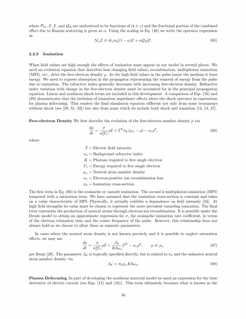
2.2.3 Ionization

When field values are high enough the effects of ionization must appear in our model in several places. Weneed an evolution equation that describes how changing field values, recombination, multiphoton ionization(MPI), etc., drive the free-electron density ρ. As the high field values in the pulse ionize the medium it losesenergy. We need to express absorption in the propagator representing the removal of energy from the pulsedue to ionization. The refractive index generally decreases with increasing free-electron density. Refractiveindex variation with change in the free-electron density must be accounted for in the principal propagationequation. Linear and nonlinear shock terms are included in this development. A comparison of Eqs. (76) and(89) demonstrates that the inclusion of ionization impedance effects alters the shock operator in expressionsfor plasma defocusing. This renders the final simulation equation different not only from some treatmentswithout shock (see [29, 31, 32]) but also from some which do include both shock and ionzation [14, 13, 27].

Free-electron Density We first describe the evolution of the free-electron number density ρ via

dρ

dt=

σ

n2oUi

ρI + IKσk (ρnt − ρ)− αrρ2, (66)

where

I = Electric field intensityno = Background refractive indexK = Photons required to free single electronUi = Energy required to free single electronρnt = Neutral atom number densityαr = Electron-positive ion recombination lossσk = Ionization cross-section.

The first term in Eq. (66) is the avalanche or cascade ionization. The second is multiphoton ionization (MPI)tempered with a saturation term. We have assumed that the ionization cross-section is constant and takeson a value characteristic of MPI. Physically, it actually exhibits a dependence on field intensity [34]. Athigh field strengths its value must be chosen to represent the more prevalent tunneling ionization. The finalterm represents the production of neutral atoms through electron-ion recombination. It is possible under theDrude model to obtain an approximate expression for σ, the avalanche ionization rate coefficient, in termsof the electron relaxation time and the center frequency of the pulse. However, this relationship does notalways hold so we choose to allow these as separate parameters.

In cases where the neutral atom density is not known precisely and it is possible to neglect saturationeffects, we may use

dρ

dt=

σ

n2oUi

ρI +βKK~ωo

IK − αrρ2, ρ ρnt (67)

per Berge [28]. The parameter βK is typically specified directly, but is related to σk and the unknown neutralatom number density via

βK = σkρntK~ωo. (68)

Plasma Defocusing As part of developing the nonlinear material model we need an expression for the timederivative of electric current (see Eqs. (15) and (16)). This term ultimately becomes what is known as the

16

plasma defocusing term. Current J is the flow of charge through a surface per unit time. The total chargeper unit volume is the product of electron number density (electrons per unit volume) and the charge perelectron. The quantity of charge flowing through a unit area is the product of total charge density and therate of flow or velocity giving

J = −eρv, (69)

where e is the charge on an electron, ρ is the total free-electron number density and v is the velocity of theflow. Differentiating both sides of Eq. (69) gives

∂J∂t

= −eρ∂v∂t. (70)

The value of the electric field is defined as [22]

E =Fq, (71)

where F is the force in Newtons and q is a quantity of charge in Coulombs. Using Eqs. (70) and (71)Newton’s second law gives

dvdt

=Fm

= − e

meE. (72)

Using Eq. (72) in Eq. (70) gives∂J∂t

=e2

meρE (73)

We must express the effect of the ionization current in Eq. (73) as an equivalent polarization for use inour nonlinear model. We may obtain the necessary expression for the integral of the current density (seeEq. (16)) most easily in the frequency domain. Using the frequency domain envelope representation wecompute the Fourier transform of the integral of the current density as

Ppls =1

(−iω)2Fe2

meρE, (74)

where division by −iω represents the effect of integration. Moving back into the slow-time (or temporalenvelope) domain we have the following expression for the plasma current equivalent polarization

Ppls = − 1(ωoT )2

e2

meρE . (75)

Expressing Eq. (75) in a form convenient for use in our nonlinear propagation equation we have

T−1NplsE = − iko2noρc

T−2(ρE), (76)

where we have used the definition of the critical plasma density

ρc ≡ εomeω2o/e

2, (77)

above which the plasma becomes opaque to waves with frequencies below ωo. Note the double shock operatorpresent in Eq. (76).

The relationship in Eq. (76) assumes electrons move in the presence of an applied electric field but doesnot take into account collisions between the electrons and the positive ions in our plasma. Drude proposed amodel for electrons in metals that assumes a sea of other particles that function as hard, essentially stationaryscattering centers. This model is certainly applicable for ionization in gases. The larger, positive ions do notrespond very much at all to an oscillating electric field. For this reason the Drude model is sometimes usedto describe this portion of the current. In particular it is needed in order to move from our instantaneousdescription in Eq. (73) to our envelope model.

17

We now develop an impedance relationship for the plasma that relates current and electric field. Theresult will be loss and delay terms that affect the propagation of the pulse. These naturally depend on thestrength of the electric field through the generation of the plasma electron density. We develop an equationfor the evolution of average electron momentum p(t). During a short time interval dt the probability thata given electron will experience a collision is approximately dt/τc where τc is known as the relaxation time(considered to be independent of the position or current velocity of the electron). This means that thechange in momentum may be written

p(t+ dt)− p(t) = −dtτc

p (78)

Eq. (78) is a simple relaxation equation. In the absence of any perturbing forces (such as electric fields), wemay write the evolution of momentum as the product of an initial value and a simple decaying exponentialwith time constant τc (hence the name relaxation time). If we have an electric field present then we simplyadd a term representing the change in momentum Fdt to arrive at

p(t+ dt)− p(t) = −dtτc

p(t) +(

1− dt

τc

)Fdt

≈ −dtτc

p(t) + Fdt, (79)

where we have neglected the second order term in dt. Finally we may divide both sides of Eq. (79) by dt,use the fact that F = −eE and take a limit as the time interval approaches zero to yield

dp(t)dt

= −p(t)τc− eE. (80)

Next we assume a time-harmonic solution to Eq. (80). Our pulses are not time-harmonic, they are envelopebased and so the relationship we obtain between the electric field and momentum (and subsequently current)will be an approximate one.

E(t) =12

[E(ω) exp(−iωt) + E∗(ω) exp(iωt)] (81)

p(t) =12

[p(ω) exp(−iωt) + p∗(ω) exp(iωt)] (82)

Substituting Eqs. (81) and (82) into Eq. (80) and solving for momentum we obtain

p(ω) =−eτc

1− iωτcE(ω) (83)

The linearity of Eq. (80) gives a separate equation for the conjugate of momentum which we don’t reallyneed. Eq. (69) tells us that we can relate momentum to current and write

J(ω) =(− eρme

)p(ω) =

(− eρme

)−eτc

1− iωτcE(ω)

≈(e2ρτcme

)1 + iωτc1 + ω2τ2

c

E(ω) (84)

Eq. (84) represents a full spectral response by the current to the electric field. The real part accounts forplasma absorption and the imaginary part for plasma defocusing. These effects vary with frequency and inorder to model the dispersive nature of the plasma impedance we would need to solve Eq. (84) at each stepand update each frequency component of the pulse accordingly. If we accept the impedance relationship atthe center frequency of the pulse as holding over the entire pulse bandwidth we may simplify Eq. (84) to

J(ω) ≈(e2ρτcme

)1 + iωoτc1 + ω2

oτ2c

E(ω), (85)

18

by replacing the general frequency variable ω with the constant ωo. We may simplify the model somewhat bycombining the nonlinear polarization and the plasma current into a single term (see Eqs. (16) and (18)) andconsider the relationship only at the center frequency of the pulse. We then require the integral of currentdensity

Ppls(ω) =J(ω)−iω

≈ − 1iω

(e2ρτcme

)1 + iωoτc1 + ω2

oτ2c

E(ω). (86)

In this case we neglect the dispersive or frequency dependent nature of the relationship between the electricfield and the integral of the current and use only the complex impedance at the center frequency of the pulse.Using the envelope representation we write the term we add to the nonlinear polarization as

Ppls = − 1iω

(e2ρτcme

)1 + iωoτc1 + ω2

oτ2c

E (87)

Now we move Eq. (87) into the slow-time domain via Eq. (43)

Ppls = − 1iωoT

(e2ρτcme

)1 + iωoτc1 + ω2

oτ2c

E (88)

as was done for the propagation Eq. (49) in section 2.1.

Using the scale factor defined in Eq. (48) we write the operator expression as

T−1NplsE ≡ −σ

2(1 + iωoτc)T−1(ρE) (89)

whereσ ≡ ko

noρc

ωoτc1 + ω2

oτ2c

, (90)

is the cross-section for inverse Bremsstrahlung (the process by which an electron absorbs energy from theoptical pulse during a collision). Note that the power of the shock operator in Eq. (89) differs from that inEq. (76).

MPI Energy Loss We need a term in our propagation equation to represent the reduction in opticalpulse energy required to ionize the medium (known as multiphoton absorption or MPA). We do this byconstructing an artificial current with the value necessary to dissipate the needed energy. This current is thecoupling between the propagation or field Eq. (49) and the ionization physics model in Eq. (66). In orderto obtain the expression for the coupling we seek the value of a current which will dissipate an amount ofpower per unit volume equal to that required to support the ionization. Remember that work is defined as

W =∫

F · dx =∫

F · v dt, (91)

and thusP =

dW

dt= F · v. (92)

By definition the force on a charge in an electric field is the product of the charge and electric field values.Hence, force per unit volume is the product of charge density and electric field value. Finally, the power perunit volume S (via Eq. (92)) is

S = −eρv ·E = J ·E, (93)

where the last equality results from the fact that the product of a density and a velocity is a flux. This maybe seen by considering a thin slice (taken normal to the velocity vector) through the density, of thickness dx.If this slice moves through its front face in time dt then it is traveling with velocity dx/dt = v. The productof the density and velocity is ρdx/dt which in our case gives how many Coulombs of charge pass through thefront face of our slice each second. If we postulate a current of the right value flowing in our electric fieldthen we will naturally have the correct power dissipation. Let us assume that the ionization rate is directly

19

proportional to the number of available neutral atoms ρnt and that we may neglect saturation effects. Wewrite

dρ

dt= Wrρnt, (94)

where Wr is the photoionization rate. This gives the number of new free electrons we should expect per unitvolume per second. For each of these electrons K photons where absorbed, each having an energy of ~ω.Hence the total energy needed per unit volume per second is given by

S = WrρntK~ωo = J ·E. (95)

This implies that the current density must be

J =WrρntK~ωo|E|2

E, (96)

where the normalization by the square of the electric field is simply to cancel the similar term in the numeratorof the dot product of current density and electric field. We have expressed everything up to now in terms ofthe instantaneous fields. Using an approximation similar to that in Eq. (58) we note that

S ≈ 12J · E (97)

and construct an expression similar to that in Eq. (96) for our developed envelope equation

J = 2WrρntK~ωo|E|2

E , (98)

where the factor of two compensates for the one-half in Eq. (97).

We need a model for the photoionization rate Wr. For a K-photon ionization process a commonly usedmodel is

Wr = σkIK , (99)

giving

J = 2σkρntK~ωoIK

|E|2E = 2

βKIK

|E|2E (100)

where we have used Eq. (68).

Just as we did in section 2.2.3 we seek a term that can be added to the polarization (even though weare modeling the loss with a current). Again, we need the integral of the current and so we use the sametechnique as we did in obtaining Eqs. (75) and (88). Expressing the relationship between current and electricfield in the frequency domain, dividing by (−iω) to obtain the integral of current and transforming back intothe slow-time temporal envelope domain we have

PMPA(r, t, z) = T−12βKIK

−iωo|E|2E , (101)

for the equivalent material polarization representing MPA. Using Eqs. (58), (48) and (101) we write

T−1NMPAE ≡ −βK2T−1IK−1E . (102)

20

3 Summary of Physical Model

Here we summarize the physical model that we discretize and solve in order to investigate various aspectsof nonlinear optical propagation. It includes paraxial diffraction, group velocity and third-order dispersion,linear and nonlinear shock, Kerr and Raman effects and ionization. There are many models for nonlinearoptical propagation in the literature [8, 9, 13, 20, 4, 18, 30, 5, 38]. Ours is similar to those in the aforemen-tioned references. However, our method of including the impedance effects in the plasma defocusing termleads to a difference in the shock terms from those in [13].

The propagation equation for the electric field envelope E is

∂ζE =i

2kT−1∇2

⊥E + iDE + TNE , (103)

with wavenumber k = 2π/λ and wavelength λ. The dispersion and shock operators are given by

D ≡ −k′′

2∂2τ − i

k′′′

6∂3τ and T ≡

(1 +

i

ωo∂τ

)(104)

respectively. The nonlinear operator may be decomposed as

N = Nkr + T−1Npls + T−1NMPA. (105)

Kerr and Raman effects are modeled with

Nkr = ikon2[(1− α)I + αQR]. (106)

We have used the approximately time-harmonic relationship

I ≈ cnoεo2|E|2 (107)

to specify the intensity envelope I. Delayed Raman response is described by

QR(r, t, z) =∫ t

−∞R(τ)I(r, t− τ, z)dτ, (108)

with

R(t) =γ2 + ω2

R

ωRexp(−γt) sin(ωRt), (109)

where ωR and γ are respectively characteristic frequency and attenuation constants for the molecular speciesinteracting with the pulse.

The following quantities

τc = Electron collision or relaxation timeme = Mass of an electronωo = Pulse center frequencyko = Pulse center wavenumberno = Background refractive indexK = Photons required to free single electronUi = Energy required to free single electronρnt = Neutral atom number densityαr = Electron-positive ion recombination lossσk = Ionization cross-section.

21

help us express the remaining ionization physics. For plasma defocusing we use

NplsE = − iko2noρc

T−1(ρE), (110)

or if we desire to include collision effects

Npls ≡ −σ

2(1 + iωoτc)ρ, (111)

withρc ≡ εomeω

2o/e

2, and σ ≡ konoρc

ωoτc1 + ω2

oτ2c

. (112)

The energy loss in the pulse due to multiphoton absorption is included via

NMPA = −βK2IK−1, (113)

withβK = σkρntK~ωo. (114)

The evolution of the electron density requires an auxiliary equation

dρ

dt=

σ

n2oUi

ρI + IKσk (ρnt − ρ)− αrρ2, (115)

ordρ

dt=

σ

n2oUi

ρI +βKK~ωo

IK − αrρ2. (116)

22

A Symbols

Symbol Units Description

εo = 8.854× 10−12 F ·m−1 Permittivity of free spaceµo = 4π × 10−7 H ·m−1 Permeability of free spacee = 1.60217657×10−19 C Magnitude of the charge carried by an electronc = 2.99792458× 108 m · s−1 Speed of light in vacuoF , F−1 − Fourier and inverse Fourier transformsE, E, E V ·m−1 Electric field (vector, scalar, envelope)E, E V ·m−1 Electric field (frequency domain scalar and envelope)H A ·m−1 Magnetic field (vector)D C ·m−2 Electric flux density (vector)B W ·m−2 Magnetic flux density (vector)J, J A ·m−2 Current density (vector, envelope)ρ C ·m−3 Electric charge densityP, Pl, Pnl C ·m−2 Vector material polarization (total, linear, nonlinear)χ(1) − Linear electric susceptibilityχ(3) − Nonlinear electric susceptibilityεr − Relative permittivityt s Time coordinate variableω rad · s−1 Angular frequencyNp C ·m−2 Total nonlinear material responsek(ω) m−1 Wavenumber as a function of angular frequencyNp C ·m−2 Fourier transform of total nonlinear material responser m Coordinate vector (x, y, z)k′ s ·m−1 First order coefficient in Taylor series expansion of k(ω)k′′ s2 ·m−1 Second order coefficient in Taylor series expansion of k(ω)k′′′ s3 ·m−1 Third order coefficient in Taylor series expansion of k(ω)k(m) sm ·m−1 mth order coefficient in Taylor series expansion of k(ω)ωo rad · s−1 Pulse center frequencyx,y m Transverse spatial coordinate variablesz m Longitudinal spatial coordinate variableζ m Retarded longitudinal spatial coordinate variableτ s Retarded temporal coordinate variableκ(ω) m−1 Sum of first two terms in Taylor series expansion of k(ω)Np C ·m−2 Fourier transform of total nonlinear material responseNp C ·m−2 Envelope of total nonlinear material responseNp C ·m−2 Fourier transform of envelope of total nonlinear material responseΩ rad · s−1 Slow frequency variable (ω − ωo)D(Ω) rad · s−1 Taylor series expansion of k(ω)− κ(ω) in slow frequency variableT ,S − Shock operatorsno − Background refractive index of materialko m−1 Central wavenumberNp m−1 Vector instantaneous nonlinear polarization response (Kerr effect)P C ·m−2 Scalar instantaneous nonlinear polarization response (Kerr effect)P C ·m−2 Scalar envelope nonlinear polarization response (Kerr effect)I W ·m−2 Scalar envelope intensityn2 m2 ·W−1 Nonlinear refractive index of materialNk m−1 Envelope Kerr operatorNkr m−1 Envelope Kerr-Raman operatorQR W ·m−2 Molecular Raman responseγ s−1 Molecular damping rate (Raman)

23

Symbol Units Description

ωR rad · s−1 Molecular Raman frequencyR(t) − Molecular impulse response (Raman)α − Raman scattering contribution to Kerr-Raman termsρ m−3 Electron number densityK − Number of electrons required to ionize atomαr m3 · s−1 Ionization recombination loss coefficientρnt m−3 Number density of neutral atomsσk WK ·m−2K · s−1 Ionization cross-section for K-photon MPI processesUi J Energy required to free an electron (ionization energy)~ J · s Planck’s constant (reduced)σ m2 Avalanche ionization rate coefficientρc m−3 Critical plasma number density (plasma is opaque for ρ > ρc)βK J ·WK ·m−2K−3 · s−1 Ionization rate coefficient (MPI)v m · s−1 VelocityF N ForcePpls C ·m−2 Plasma current equivalent polarizationNpls C ·m−2 Plasma current equivalent polarization operatorτc s Electron collision or relaxation timep(t) kg ·m · s−2 Electron momentumPpls C ·m−2 Fourier transform of plasma current equivalent polarizationW J WorkP J · s−1 PowerS J · s−1 ·m−3 Power per unit volumeS J · s−1 ·m−3 Envelope power per unit volumeWr s−1 Power per unit volumePMPA C ·m−2 MPA equivalent polarizationNMPA C ·m−2 MPA envelope operator

24

References

[1] L. Berge A. Couairon. Modeling the filamentation of ultra-short pulses in ionizing media. Phys. Plasmas,(1):193–209, 7 2000.

[2] L. Berge A. Couairon. Modeling the filamentation of ultra-short pulses in ionizing media. Phys. Plasma,7(1):193–209, 2000.

[3] Govind P. Agrawal. Nonlinear Fiber Optics. Optics and Photonics. Academic Press, San Diego, thirdedition, 2001.

[4] N. Akozbek, A. Iwasaki, A. Becker, M. Scalora, S.L. Chin, and C.M. Bowden. Third-harmonic gen-eration and self-channeling in air using high-power femtosecond laser pulses. Physical Review Letters,89(14):143901/1 – 4, September 2002.

[5] L. Berge, S. Skupin, R. Nuter, J. Kasperian, and J-P Wolf. Ultrashort filaments of light in weaklyionized, optically transparent media. Rep. Prog. Phys., 70:1633–1713, 2007.

[6] M. Born and E. Wolf. Principles of Optics: Electromagnetic Theory of Propagation, Interference andDiffraction of Light. Cambridge University Press, 1999.

[7] Robert W. Boyd. Nonlinear Optics. Elsevier Science, 1992.

[8] T. Brabec and F. Krausz. Intense few-cycle laser fields: Frontiers of nonlinear optics. Reviews of ModernPhysics, 72(2):545 – 91, April 2000.

[9] Thomas Brabec and Ferenc Krausz. Nonlinear optical pulse propagation in the single-cycle regime.Phys. Rev. Lett., 78(17):3283–3285, April 1997.

[10] R. N. Bracewell. The Fourier Transform and its Applications, volume 42. McGraw-Hill, 1986.

[11] G. Cerullo and S. De Silvestri. Ultrafast optical parametric amplifiers. Review of Scientific Instruments,74(1):1–18, 2003.

[12] A. Couairon, E. Brambilla, T. Corti, D. Majus, O. de J. Ramirez-Gongora, and M. Kolesik. Practitionersguide to laser pulse propagation models and simulation. Eur. Phys. J. Special Topics, (199):5–76, 2011.

[13] A. Couairon and A. Mysyrowicz. Femtosecond filamentation in transparent media. Physics Reports,441(2-4):47 – 189, 2007.

[14] A. Couairon, S. Tzortzakis, L. Berge, M. Franco, B. Prade, and A. Mysyrowicz. Infrared light filaments:simulations and experiments. J. Opt. Soc. Am. B, 19:1117, 2002.

[15] Jean-Claude Diels and Wolfgang Rudolph. Ultrashort Laser Pulse Phenomena: fundamentals, tech-niques, and applications on a femtosecond time scale. Optics and Photonics. Academic Press, SanDiego, first edition, 1996.

[16] Jerrold e. Marsden and Anthony J. Tromba. Vector Calculus. W.H. Freeman and Company, 1998.

[17] M.D. Feit and Jr. J.A. Fleck. Beam nonparaxiality, filament formation, and beam breakup in theself-focusing of optical beams. J. Opt. Soc. Am. B, 5(3):633–640, March 1988.

[18] G. Fibich. Self-focusing in the damped nonlinear Schrodinger equation. SIAM J. Appl. Math., 61(5):1680– 1705, 2001.

[19] P. A. Franken, A. E. Hill, C. W. Peters, and G. Weinreich. Generation of optical harmonics. Phys. Rev.Lett., 7(4-15):118–119, August 1961.

[20] Alexander L. Gaeta. Nonlinear propagation and continuum generation in microstructured optical fibers.Opt. Lett., 27(11):924–926, June 2002.

25

[21] H. M. Gibbs, S. L. McCall, and T. N. C. Venkatesan. Differential gain and bistability using a sodium-filled fabry-perot interferometer. Phys. Rev. Lett., 36:1135–1138, May 1976. First demonstration andexplanation of optical bistability.

[22] David Halliday and Robert Resnick. Fundamental Physics. John Wiley & Sons, 2e edition, 1986.

[23] J. Hansryd, P.A. Andrekson, M. Westlund, Jie Li, and P. Hedekvist. Fiber-based optical parametricamplifiers and their applications. Selected Topics in Quantum Electronics, IEEE Journal of, 8(3):506–520, 2002.

[24] Akira Hasegawa and Frederick Tappert. Transmission of stationary nonlinear optical pulses in dispersivedielectric fibers. i. anomalous dispersion. Applied Physics Letters, 23(3):142–144, 1973. Theoreticalprediction of soliton.

[25] Akira Hasegawa and Frederick Tappert. Transmission of stationary nonlinear optical pulses in disper-sive dielectric fibers. ii. normal dispersion. Applied Physics Letters, 23(4):171–172, 1973. Theoreticalprediction of soliton.

[26] John David Jackson. Classical Electrodynamics. John Wiley & Sons, New York, 1999.

[27] Mahesh R. Junnarkar. Short pulse propagation in tight focusing conditions. Optics Comm., 195(1–4):273–292, August 2001.

[28] A. Couairon L. Berge. A variational method for extended nonlinear schroedinger systems. Physica D,pages 152–153, 2001.

[29] M. Mlejnek, M. Kolesik, J. V. Moloney, and E. M. Wright. Optically turbulent femtosecond light guidein air. Phys. Rev. Lett., 83:2938–2941, Oct 1999.

[30] M. Mlejnek, M. Kolesik, E.M. Wright, and J.V. Moloney. Recurrent femtosecond pulse collapse in airdue to plasma generation: numerical results. Mathematics and Computers in Simulation, 56(6):563 –70, July 2001.

[31] M. Mlejnek, E. M. Wright, and J. V. Moloney. Dynamic spatial replenishment of femtosecond pulsespropagating in air. Opt. Lett., 23(5):382–384, March 1998.

[32] M. Mlejnek, E. M. Wright, and J. V. Moloney. Femtosecond pulse propagation in Argon: A pressuredependence study. Phys. Rev. E, 58(4):4903–4910, Oct 1998.

[33] Linn F. Mollenauer. The non-linear Schrodinger equation and ordinary solitons. Unpublished presen-tation (Lucent Technologies), 2002.

[34] Jens Schwarz, Patrick Rambo, Mark Kimmel, and Briggs Atherton. Measurement of nonlinear refractiveindex and ionization rates in air using a wavefront sensor. Optics Express, 20(8):8791–8803, apr 2012.

[35] Richard L. Sutherland. The Handbook of Nonlinear Optics. Marcel Dekker, 2003.

[36] R. W. Terhune, P. D. Maker, and C. M. Savage. Optical harmonic generation in calcite. Phys. Rev.Lett., 8:404–406, May 1962. First observation of third order harmonic generation.

[37] E.J. Woodbury and W.K. Ng. Ruby laser operation in the near IR. Proc. IRE, 50(11):2365–2383, nov1962. First observation of optical Raman scattering.

[38] A.A. Zozulya, S.A. Diddams, A.G. Van Engen, and T.S. Clement. Propagation dynamics of intensefemtosecond pulses: multiple splittings coalescence and continuum generation. Physical Review Letters,82(7):1430 – 3, February 1999.

[39] Alex A. Zozulya. Propagation dynamics of intense femtosecond pulses: multiple splittings, coalescence,and continuum generation. Phys. Rev. Lett., 82(7), 1999.

[40] Alex A. Zozulya, Scott A. Diddams, and Tracy S. Clement. Investigations of nonlinear femtosecondpulse propagation with the inclusion of Raman, shock, and third-order phase effects. Phys. Rev. A,58(4):3303–3310, October 1998.

26

DISTRIBUTION:

1 MS 0359 D. Chavez, LDRD Office, 19111 MS 0899 Technical Library, 9536 (electronic copy)

27

v1.40

29

Derivation of an Applied Nonlinear Schroedinger...

Documents

Transcript of Derivation of an Applied Nonlinear Schroedinger...