SANDIA REPORT SAND2015-5879 Unlimited Release Printed July 2015

Development and Evaluation of a Sandia Cooler-based Refrigerator Condenser

Program Manager: Thomas E. Felter

Authors: Terry A. Johnson, Arthur Kariya, Michael T. Leick, and Mark Zimmerman Energy Innovation Department 8366

Manjie Li, Yilin Du, Hoseong Lee, Yunho Hwang, Reinhard Radermacher Center for Environmental Energy Engineering, Department of Mechanical Engineering University of Maryland Prepared by Sandia National Laboratories Albuquerque, New Mexico 87185 and Livermore, California 94550

Sandia National Laboratories is a multi-program laboratory managed and operated by Sandia Corporation, a wholly owned subsidiary of Lockheed Martin Corporation, for the U.S. Department of Energy's National Nuclear Security Administration under contract DE-AC04-94AL85000. Approved for public release; further dissemination unlimited.

2

Issued by Sandia National Laboratories, operated for the United States Department of Energy

by Sandia Corporation.

NOTICE: This report was prepared as an account of work sponsored by an agency of the

United States Government. Neither the United States Government, nor any agency thereof,

nor any of their employees, nor any of their contractors, subcontractors, or their employees,

make any warranty, express or implied, or assume any legal liability or responsibility for the

accuracy, completeness, or usefulness of any information, apparatus, product, or process

disclosed, or represent that its use would not infringe privately owned rights. Reference herein

to any specific commercial product, process, or service by trade name, trademark,

manufacturer, or otherwise, does not necessarily constitute or imply its endorsement,

recommendation, or favoring by the United States Government, any agency thereof, or any of

their contractors or subcontractors. The views and opinions expressed herein do not

necessarily state or reflect those of the United States Government, any agency thereof, or any

of their contractors.

Printed in the United States of America. This report has been reproduced directly from the best

available copy.

Available to DOE and DOE contractors from

U.S. Department of Energy

Office of Scientific and Technical Information

P.O. Box 62

Oak Ridge, TN 37831

Telephone: (865) 576-8401

Facsimile: (865) 576-5728

E-Mail: reports@osti.gov

Online ordering: http://www.osti.gov/scitech

Available to the public from

U.S. Department of Commerce

National Technical Information Service

5301 Shawnee Rd

Alexandria, VA 22312

Telephone: (800) 553-6847

Facsimile: (703) 605-6900

E-Mail: orders@ntis.gov

Online order: http://www.ntis.gov/search

3

SAND2015-5879

Unlimited Release

Printed July 2015

Development and Evaluation of a Sandia Cooler-based Refrigerator Condenser

T. A. Johnson, A. Kariya, M. T. Leick, and M. D. Zimmerman

Energy Innovation

Sandia National Laboratories

P.O. Box 969

Livermore, California 94550

M. Y. Li, Y. Du, H.H. Lee, Y.Y. Hwang, R.R. Radermacher

Center for Environmental Energy Engineering

Department of Mechanical Engineering

University of Maryland

College Park, MD 20742-3035

Abstract

This report describes the first design of a refrigerator condenser using the Sandia Cooler, i.e. air-

bearing supported rotating heat-sink impeller. The project included baseline performance testing

of a residential refrigerator, analysis and design development of a Sandia Cooler condenser

assembly including a spiral channel baseplate, and performance measurement and validation of

this condenser system as incorporated into the residential refrigerator. Comparable performance

was achieved in a 60% smaller volume package. The improved modeling parameters can now be

used to guide more optimized designs and more accurately predict performance.

4

ACKNOWLEDGMENTS

The authors thank Imane Khalil and Daniel Matthew for their early significant contributions to

this project.

5

CONTENTS

Acknowledgments........................................................................................................................... 4

Contents .......................................................................................................................................... 5

Figures............................................................................................................................................. 6

Tables .............................................................................................................................................. 8

Nomenclature ................................................................................................................................ 10

1 Introduction ............................................................................................................................. 12 1.1 Background ................................................................................................................... 12 1.2 Objectives ..................................................................................................................... 13 1.3 Approach ....................................................................................................................... 13

2 Experimental Setup ................................................................................................................. 14 2.1 Test Standard and Procedure ........................................................................................ 14

2.2 Test Unit and Instrumentation ...................................................................................... 16 2.2.1 Test Unit.......................................................................................................... 16 2.2.2 Instrumentation ............................................................................................... 18

2.3 Data Reduction.............................................................................................................. 24 2.4 Uncertainty Analysis ..................................................................................................... 25

3 Sandia Cooler Condenser Development ................................................................................. 26 3.1 Conceptual Design ........................................................................................................ 26 3.2 Base Plate Design ......................................................................................................... 28

3.2.1 Heat Transfer Analysis ................................................................................... 30 3.2.2 Pressure Drop Analysis ................................................................................... 34

3.2.3 Base Plate Fabrication..................................................................................... 36 3.3 Impeller Design and Fabrication ................................................................................... 38

3.4 Start-up System ............................................................................................................. 39 3.5 Motor and Controller .................................................................................................... 40

3.5.1 Motor Selection ............................................................................................... 40 3.5.2 Controller Selection ........................................................................................ 45 3.5.3 Control Module ............................................................................................... 45

3.6 Shroud Design ............................................................................................................... 47

3.7 Final Assembly ............................................................................................................. 48

4 Test Results ............................................................................................................................. 53 4.1 Baseline Test as Shipped .............................................................................................. 53

4.1.1 Medium Temperature Setting ......................................................................... 53

4.1.2 Warmest Temperature Setting ........................................................................ 56 4.2 Baseline Test with Full Instrumentation ....................................................................... 60

4.2.1 Refrigerant Charge Optimization .................................................................... 61

4.2.2 Medium Temperature Setting Results ............................................................ 62 4.2.3 Warmest Temperature Setting ........................................................................ 66 4.2.4 Testing Repeatability ...................................................................................... 68

4.3 Sandia Cooler Condenser Test ...................................................................................... 68 4.3.1 Refrigerant Charge Optimization .................................................................... 70

6

4.3.2 Effect of rpm ................................................................................................... 73

4.4 Discussion ..................................................................................................................... 74 4.4.1 Predicted vs. Measured Performance .............................................................. 74 4.4.2 Comparison to baseline condenser.................................................................. 80

5 Conclusions ............................................................................................................................. 83 5.1 Future Work .................................................................................................................. 85

6 References ............................................................................................................................... 86

7 Distribution ............................................................................................................................. 87

FIGURES Fig. 1.1: Sandia Cooler ................................................................................................................. 13

Fig. 1.2: Approach for Sandia Cooler Evaluation......................................................................... 14

Fig. 2.1: Definition of defrost test period [3] ................................................................................ 15 Fig. 2.2: Back view of the natural convection refrigerator condenser [6] .................................... 16

Fig. 2.3: Back view of the testing unit .......................................................................................... 17 Fig. 2.4: Volume of fan and condenser together ........................................................................... 17

Fig. 2.5: Schematic of instruments installation on refrigeration-side ........................................... 18 Fig. 2.6: Air-side, surface, in-stream T-type thermocouples (left to right) .................................. 20 Fig. 2.7: Surface thermocouples for air side temperature measurement ....................................... 20

Fig. 2.8: Instream thermocouple for refrigerant side temperature measurement .......................... 20 Fig 2.9: Thermocouples installed in the system when testing as shipped .................................... 21

Fig. 2.10: Locations of thermocouples measuring compartment temperature.............................. 21 Fig. 2.11: Pictures of thermocouples in fresh food (left) and freezer (right) compartments ........ 22

Fig. 2.12: Locations of thermocouples measuring ambient temperature (top-view (left); side-view

(right)) ........................................................................................................................................... 22

Fig. 2.13: Pressure transducers used in the test ............................................................................ 23 Fig. 2.14: Differential pressure transducer used to measure the condenser pressure drop. .......... 23 Fig. 2.15: Mass flow meter and the transmitter (left to right)....................................................... 24

Fig. 3.1: Side-by-side configuration ............................................................................................. 27

Fig. 3.2: Back-to-back configuration ............................................................................................ 27 Fig. 3.3: Initial refrigerant channel concept .................................................................................. 28 Fig. 3.4: Spiral channel concept .................................................................................................... 28 Fig. 3.5: Cross-sectional view of the baseplate. The inset shows the dimension nomenclature for

the channel geometry. ................................................................................................................... 29

Fig. 3.6: COMSOL simulation of the effect of channel wall thickness ........................................ 31 Fig. 3.7: Comparison of different heat transfer coefficient correlation with experiment data for

R134a ............................................................................................................................................ 33 Fig. 3.8: Comparison of different pressure drop correlation with experiment data for R134a ..... 35 Fig. 3.9: Components of the baseplate: the main plate and lid. All channel features are machined

into the main plate. The machined channel is closed by brazing the main plate and lid together 37 Fig. 3.10: Top-view of the completed baseplate ........................................................................... 37

Fig. 3.11: Access ports in the baseplate ....................................................................................... 38 Fig. 3.12: Pictures of one of the Sandia Cooler impellers ............................................................ 39 Fig. 3.13: Timing diagram for start-up ......................................................................................... 40

7

Fig. 3.14: Motrolfly motor assembly ............................................................................................ 41

Fig. 3.15: DLRK Winding ............................................................................................................ 41 Fig. 3.16: Torque-speed curve ...................................................................................................... 42 Fig. 3.17: Hysteresis Brake setup ................................................................................................ 43

Fig. 3.18: Torque output vs. power consumption at 2000 rpm with 25V supply ......................... 44 Fig. 3.19: Electrical to mechanical efficiency vs. torque output at 2000 rpm with 25 V supply . 45 Fig. 3.20: Front/Rear panel ........................................................................................................... 46 Fig. 3.21: Controller Block Diagram ............................................................................................ 47 Fig. 3.22: Exploded view of main shroud components ................................................................ 48

Fig. 3.23: SCC assembly ............................................................................................................... 49 Fig. 3.24: Cross-section of the SCC assembly .............................................................................. 49 Fig. 3.25: Motor stator and shaft assembled to the baseplate ....................................................... 50 Fig. 3.26: One impeller mounted to the baseplate ........................................................................ 50

Fig. 3.27: Eddy current sensor used to set the impeller air gaps .................................................. 51 Fig. 3.28: Fully assembled Sandia Cooler condenser ................................................................... 52

Fig. 3.29: Mounting configuration ................................................................................................ 52 Fig. 4.1: Variation of temperatures and power consumption (“stabilization” at Tamb=32.2°C and

medium temperature setting) ........................................................................................................ 53 Fig. 4.2: Variation of surface temperatures on refrigerant-side (“stabilization” at Tamb=32.2°C

and medium temperature setting).................................................................................................. 54

Fig 4.3: Variation of temperatures and power consumption (“defrost” at Tamb=32.2°C and

medium temperature setting) ........................................................................................................ 54

Fig 4.4: Variation of surface temperatures on refrigeration-side (“defrost” at Tamb=32.2°C and

medium temperature setting) ........................................................................................................ 55 Fig. 4.5: Variation of temperatures and power consumption (“stabilization” at Tamb=32.2°C and

warmest temperature setting) ........................................................................................................ 57

Fig. 4.6: Variation of surface temperatures on refrigeration-side (“stabilization” at Tamb=32.2°C

and medium temperature setting).................................................................................................. 57 Fig. 4.7: Variation of temperatures and power consumption (“defrost” at Tamb=32.2°C and

warmest temperature setting) ........................................................................................................ 58 Fig. 4.8: Variation of surface temperatures on refrigeration-side (“defrost” at Tamb=32.2°C and

medium temperature setting) ........................................................................................................ 58 Fig. 4.9: Schematic diagram of the system ................................................................................... 61

Fig. 4.10: Instruments installed in the experiment set up ............................................................. 61 Fig. 4.11: Variation of temperatures and power consumption (“stabilization” at Tamb=32.2°C and

medium temperature setting) – test with full instruments ............................................................ 63 Fig. 4.12: Variation of temperatures on refrigeration-side (“stabilization” at Tamb=32.2°C and

medium temperature setting) – test with full instruments ............................................................ 63

Fig. 4.13 Variation of pressure and pressure drop (“stabilization” at Tamb=32.2°C and medium

temperature setting) ...................................................................................................................... 64

Fig. 4.14 Variation of mass flow rate (“stabilization” at Tamb=32.2°C and medium temperature

setting)........................................................................................................................................... 65 Fig. 4.15 Variation of condenser sub-cool and suction line superheat (“stabilization” at

Tamb=32.2°C and medium temperature setting) ............................................................................ 65 Fig. 4.16: Variation of temperatures and power consumption (“stabilization” at Tamb=32.2°C and

warmest temperature setting) ........................................................................................................ 67

8

Fig. 4.17: Scheme #1: SCC in the refrigerator unit ...................................................................... 69

Fig. 4.18: Scheme #2: SCC out of the refrigerator unit ................................................................ 69 Fig. 4.19: Variation of pressure and pressure drop (“stabilization” at medium temperature setting

for system charge of 113g) ........................................................................................................... 70

Fig. 4.20: Variation of pressure and pressure drop (“stabilization” at medium temperature setting

for system charge of 125g) ........................................................................................................... 71 Fig. 4.21: Variation of temperatures and power consumption (“stabilization” at medium

temperature setting, 125 g charge, rpm is fixed at 1400) .............................................................. 73 Fig. 4.22: Refrigerant mass flow rate for SCC (1400 rpm; medium temperature setting) ........... 77

Fig. 4.23: Dimensions for the SCC (left) and conventional tube-fin heat exchanger and fan (right)

....................................................................................................................................................... 82 Fig. 4.24. Pressure drop of baseline tube-fin condenser and SCC ................................................ 83

TABLES

Table 2.1: Specifications of Selected Frigidaire Unit ................................................................... 17 Table 2.2: Specifications of instruments ....................................................................................... 19

Table 2.3: Calculation of systematic uncertainties ....................................................................... 25 Table 3.1: Operating conditions used to design the baseplate refrigerant channel geometry. ..... 30 Table 3.2: Dimensions of the baseplate refrigerant channel geometry, as shown in Fig. 3.5. The

channel length is the outer length of the spiral. ............................................................................ 30 Table 3.3: Refrigeration-side heat transfer analysis for baseplate design .................................... 34

Table 3.4: Refrigeration side heat transfer analysis for baseplate design ..................................... 36 Table 3.5: DM2205-390 Brake torque test at 2000 rpm and Vsupply = 25V .................................. 44 Table 3.6: Air bearing gap settings ............................................................................................... 51

Table 4.1: Air-side data at medium temperature setting ............................................................... 55

Table 4.2: Refrigerant temperature at medium temperature setting ............................................. 56 Table 4.3: Air side specifications of test data at warmest temperature setting ............................. 59 Table 4.4: Condenser related surface temperature at warmest temperature setting ..................... 59

Table 4.5: Summary of test data in “test as shipped” ................................................................... 60 Table 4.6: Charging optimization for a complete cycle ................................................................ 62

Table 4.7: Charging optimization for one compressor-on time .................................................... 62 Table 4.8: Air side test data at medium temperature setting (stabilization) ................................. 66 Table 4.9 Condenser related temperature at medium temperature setting (stabilization) ............ 66 Table 4.10: Summary of test data in “Test with full instruments” ............................................... 67

Table 4.11: Result of repeat test (stabilization at medium temperature setting) .......................... 68 Table 4.12 Comparison of airside condition for scheme #1 and #2 ............................................ 70 Table 4.13: Cabinet temperatures and cycle time comparison (Stabilization at medium

temperature setting, rpm is fixed at 1400) .................................................................................... 71 Table 4.14: Energy consumption of different charges for six stabilization cycles (medium

temperature setting, rpm is fixed at 1400) .................................................................................... 72 Table 4.15: Properties of optimized charge (instantaneous values before the compressor turns off,

medium temperature setting, rpm is fixed at 1400) ...................................................................... 72 Table 4.16: Energy consumption of different rotational speed for six stabilization cycles

(medium temperature setting, refrigerant charge is 125g for Sandia Cooler) .............................. 73

9

Table 4.17: Properties of different rotational speed (instantaneous values before the compressor

turns off, medium temperature setting, 125g charge for Sandia Cooler tests) ............................. 74 Table 4.18: Measured air-side thermal resistance ......................................................................... 75 Table 4.19: Calculated air-side thermal resistance ....................................................................... 75

Table 4.20: Refrigerant-side heat transfer from Sandia Cooler condenser tests (1400 rpm; mass

flow = 1 g/s) .................................................................................................................................. 77 Table 4.21: Analysis of refrigerant channel length based on measured temperatures and predicted

heat transfer coefficients for each phase ....................................................................................... 79 Table 4.22. Predicted and measured pressure drop for the SCC (1400 rpm; 125 g charge)......... 79

Table 4.23: Air side heat transfer performance comparison (Stabilization at medium temperature

setting)........................................................................................................................................... 81 Table 4.24: Size and normalized heat transfer comparison .......................................................... 82

10

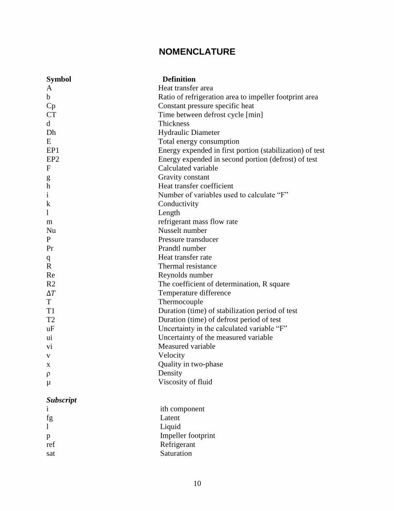
NOMENCLATURE

Symbol Definition A

b

Cp

CT

d

Dh

E

EP1

EP2

F

g

h

i

k

l

m

Nu

P

Pr

q

R

Re

R2

∆𝑇 T

T1

T2

uF

ui

vi

v

x

ρ

µ

Heat transfer area

Ratio of refrigeration area to impeller footprint area

Constant pressure specific heat

Time between defrost cycle [min]

Thickness

Hydraulic Diameter

Total energy consumption

Energy expended in first portion (stabilization) of test

Energy expended in second portion (defrost) of test

Calculated variable

Gravity constant

Heat transfer coefficient

Number of variables used to calculate “F”

Conductivity

Length

refrigerant mass flow rate

Nusselt number

Pressure transducer

Prandtl number

Heat transfer rate

Thermal resistance

Reynolds number

The coefficient of determination, R square

Temperature difference

Thermocouple

Duration (time) of stabilization period of test

Duration (time) of defrost period of test

Uncertainty in the calculated variable “F”

Uncertainty of the measured variable

Measured variable

Velocity

Quality in two-phase

Density

Viscosity of fluid

Subscript

i

fg

l

p

ref

sat

ith component

Latent

Liquid

Impeller footprint

Refrigerant

Saturation

11

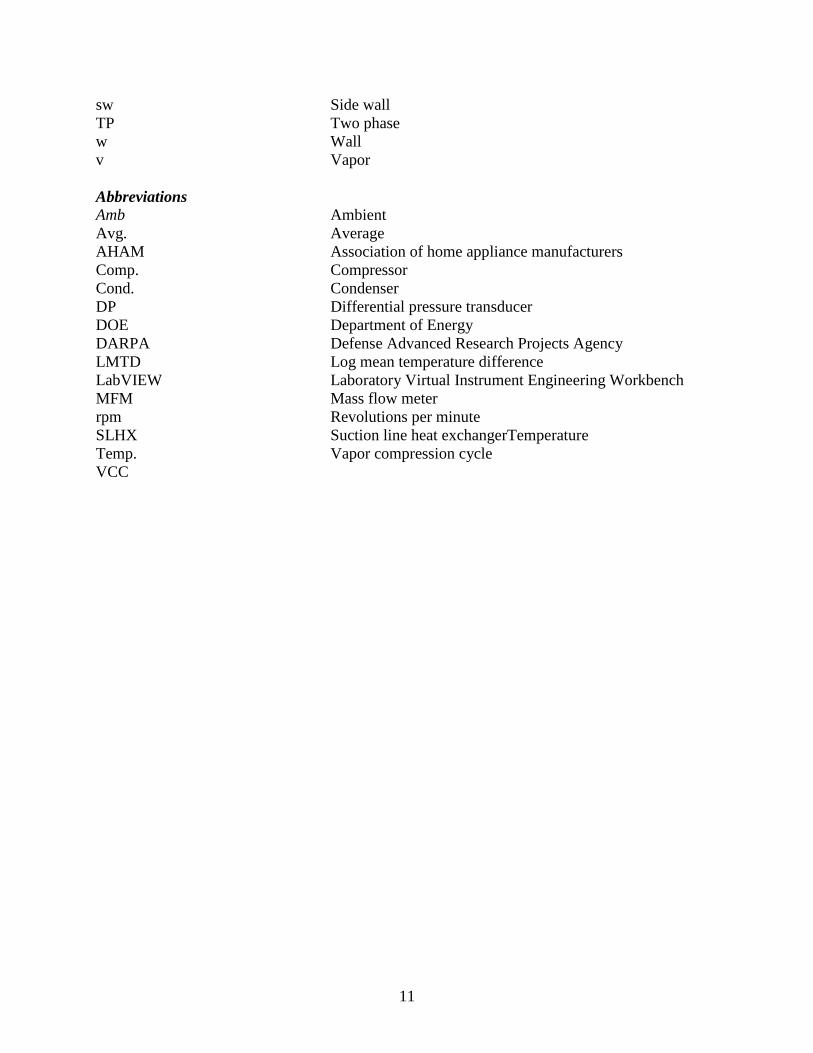
sw

TP

w

v

Side wall

Two phase

Wall

Vapor

Abbreviations

Amb

Avg.

AHAM

Comp.

Cond.

DP

DOE

DARPA

LMTD

LabVIEW

MFM

rpm

SLHX

Temp.

VCC

Ambient

Average

Association of home appliance manufacturers

Compressor

Condenser

Differential pressure transducer

Department of Energy

Defense Advanced Research Projects Agency

Log mean temperature difference

Laboratory Virtual Instrument Engineering Workbench

Mass flow meter

Revolutions per minute

Suction line heat exchangerTemperature

Vapor compression cycle

12

1 INTRODUCTION

1.1 Background Improving the performance and reducing the size of heat exchangers in air conditioners,

heat pumps, and refrigerators is a the subject of much current research and development. A

typical air-to-refrigerant heat exchanger is assembled with a fan, a so-called “fan-plus-finned

heat exchanger”. Fins are applied to increase the heat transfer area, and the air is driven by the

fan. However, there are inherent limitations to further improve heat exchanger performance in

terms of the equipment size, noise and cost. The current typical air-cooled heat exchangers have

the following challenges:

Large volume: heat exchanger and fan together

Limitation on increasing fan air flow rate due to noise, power and cost

High thermal resistance, low heat transfer efficiency

High power consumption

To overcome these issues, researchers have investigated different fin types and different heat

exchanger geometries. However, total performance improvements are very limited because the

thermal resistance mainly lies in the air-side. Improvements to the air-side heat transfer

coefficient could lead to a more efficient heat exchanger unit. The primary physical limitation to

performance (i.e. low thermal resistance) is the boundary layer of motionless air that adheres to

and envelops all surfaces of the heat exchanger [1]. Within this boundary layer, molecular

diffusion is the primary transport mechanism for heat conduction, much worse than convective

heat transfer considering the low thermal conductivity of the air. There are several ways to

decrease this boundary layer effect, for example to increase the surface velocity. However, this

means a larger fan is needed, which will consume more energy.

To address this problem, a fundamentally different approach to air-cooled heat exchangers was

developed at Sandia National Laboratories [1, 2] called the Sandia Cooler. Fig. 1.1 shows the

latest version of the Sandia Cooler. The key to the technology is the heat-sink impeller which

consists of a disc-shaped impeller populated with fins on its top surface. The impeller functions

like a hybrid of a conventional finned metal heat sink and a fan. Air is drawn in the downward

direction into the central region having no fins, and expelled in the radial direction through the

dense array of fins. A high efficiency brushless motor is used to impart rotation (~2000 rpm) to

the heat-sink-impeller. Originally developed for electronics cooling, the underside of the

baseplate is mounted to a heat source. Heat flows through the baseplate, thin hydrodynamic air

bearing gap (0.01 mm), impeller base, and impeller fins and is transferred to surrounding airflow.

Radial acceleration of the airflow over the finned surfaces thins the boundary layer and enhances

air-side heat transfer compared to conventional fan and fin devices [1]. Due to the rotation of the

heat transfer surfaces, the Sandia Cooler is also inherently resistant to fouling. Finally, by

integrating the fan and the heat exchanger, each of which is a source of noise in a conventional

heat exchanger, improvements in overall noise level can be expected.

13

Fig. 1.1: Sandia Cooler

1.2 Objectives In this research project, the Sandia Cooler concept is applied to a household refrigerator

condenser. Conventional condensers usually consist of a fan and copper or aluminum coils and

take up a relatively large space. There are two main advantages of the Sandia Cooler condenser

(SCC) for the refrigerator application: compact geometry and improved air-side heat transfer

performance. Previously, the Sandia Cooler concept has been applied primarily to computer CPU

cooling. For the refrigerator condenser application, the heat source temperature is relatively low.

This means that the device needs more heat transfer area to obtain the required heat transfer

capacity with a smaller temperature difference. Therefore, a new design must be investigated and

optimized. The main objective of this project is to apply the novel Sandia Cooler concept to a

refrigerator condenser application. The project is therefore exploratory in nature and includes

four main tasks as follows:

Establish a baseline performance level for comparison through testing

Design the SCC including a new heat exchanger baseplate with refrigerant flow channels

Confirm operation of the SCC and validate the design through testing and compare to the

baseline

Assess the SCC performance and recommend improvements

1.3 Approach To investigate the performance potential of the Sandia Cooler, the approach was divided

into three steps as shown in Fig. 1.2. The first step is the baseline test, which establishes the

baseline performance of a residential refrigerator. The operating conditions obtained from the

baseline test are used for designing the SCC. The refrigerator unit is tested as shipped without

changing the refrigerant-side. The yearly energy consumption is compared with manufacturer

claims to ensure our test procedure is accurate. In this sub-task, no intrusive instrument is

installed. After that, the refrigeration-side is opened up so that sensors can be installed, such as

pressure sensors, a mass flow meter and in-stream thermocouples. This provides detailed

14

operating conditions of the test unit. In the second step (design), the data from the baseline tests

are used as a design condition for the Sandia Cooler heat exchanger. Once a design is chosen,

heat transfer and pressure drop are evaluated and performance is determined. The final step is to

validate the design with the SCC installed in the refrigerator. The system is modified to use the

Sandia Cooler, tested and compared with the baseline results.

Fig. 1.2: Approach for Sandia Cooler Evaluation

2 EXPERIMENTAL SETUP

2.1 Test Standard and Procedure Refrigerator tests were conducted based on the DOE standard, Uniform Test Method for

Measuring the Energy Consumption of Electric Refrigerators and Electric Refrigerator-

Freezers, Appendix A1 to Subpart B of Part 430, 10 CFR Ch. 2 (1-1-2012 Edition) [3]. The DOE

standard includes some regulations that refer to the AHAM standard [4] which is also referenced

in the test procedures. In the 2012 edition of the DOE standard, the testing unit should be at an

ambient temperature of 32.2 ±0.6°C, which is higher than what would be expected in an average

household. This higher ambient temperature allows for an approximation of the cabinet heat

losses without needing to simulate cabinet door openings, which tend to be difficult and

expensive to implement reliably. The test unit used was a typical top-freezer refrigerator, which

falls into the category of “refrigerator-freezer with long-time automatic defrost control”.

The unit was first tested under the medium temperature setting and the temperatures of

both compartments were compared to the standard temperatures. For an electric refrigerator-

freezer, the standard temperature for the freezer compartment is -15°C and for the fresh food

compartment it is 7.2°C. If the compartment temperatures for the medium setting are both lower

15

than these standardized temperature, then a second test is conducted under the warmest

temperature setting. If the temperatures are higher than the standard, the second test is conducted

under the coldest temperature setting. The energy consumption for each test are recorded and

used for estimating yearly energy consumption.

There are two parts for each of the tests listed above: one is a temperature stabilization part

and the other is a defrost cycle. Temperature stabilization is defined as when the compressor

on/off cycles do not change relative to one another. According to the DOE standard [3], during

this “steady-state” condition the temperature measurements in the cabinets are not changing by

more than 0.023°C per hour. For the purposes of consistency and repeatability, all of the DOE

testing results for yearly energy consumption are calculated from six complete on and off cycles.

The defrost cycle is measured from the end of the last compressor on-cycle before the “precool”

cycle occurs to the end of the recovery cycle after the defrost period. Sometimes there is a

“precool” cycle before the defrost heater turns on, this extended on-cycle is to ensure the freezer

compartment remains at a low temperature through the defrost cycle in order to protect the food

from thawing. When the defrost heater turns on, an electrical resistance is used to heat the

evaporator to a temperature high enough to melt and remove the frost. Although the heater may

only be on for 10 to 20 minutes, the defrost test period is longer because the effect lasts well after

the heater turns off. As shown in Fig. 2.1, the defrost test begins at the end of one normal cycle,

contains the defrost heater period and recovery cycle, and ends at the beginning of the regular

compressor cycle.

Fig. 2.1: Definition of defrost test period [3]

16

2.2 Test Unit and Instrumentation

2.2.1 Test Unit In the United States, there are many types of refrigerators: top-freezer, bottom freezer,

side-by-side, and French door style refrigerators. The market share for the top-freezer

refrigerator is 70 percent and that for the side-by-side model is 25 percent. However, with the

increase in consumer’s needs, the market share for side-by-side models and French door style

models is increasing [5].

There are two types of air cooled refrigerator condensers: natural convection and forced

convection condensers. In a natural convection condenser, air flow is buoyancy driven due to

temperature gradients in the condenser coil. In a forced convection condenser, a motor-driven

fan blows air over the condenser coil. Fig. 2.2 and Fig. 2.3 show the back views of these two

condensers. Because a forced convection type condenser is more compact and suitable to be

replaced by a SCC, the unit with forced convection was used in the test.

An 18.2 cubic feet top-freezer refrigerator from Frigidaire was selected as the test unit (model

number: FFHT1826LW). This refrigerator has a 4.07 cubic feet freezer capacity and 14.13 cubic

feet fresh food compartment. The manufacturer claims that the yearly energy consumption for

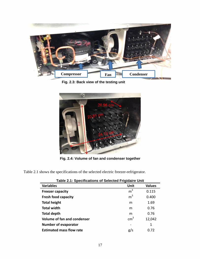
this unit is 383 kWh. Fig. 2.3 shows the back view of the test unit; from left to right are the

compressor, fan and condenser. When the refrigerator is running, a cardboard panel covers the

back to enable a specific air flow direction. The air is supplied from the right, cools the

condenser first, and then cools the compressor. Fig. 2.4 shows detailed dimensions of the fan and

condenser together. The estimated volume is 12,042 cm3.

Fig. 2.2: Back view of the natural convection refrigerator condenser [6]

17

Fig. 2.3: Back view of the testing unit

Fig. 2.4: Volume of fan and condenser together

Table 2.1 shows the specifications of the selected electric freezer-refrigerator.

Table 2.1: Specifications of Selected Frigidaire Unit

Variables Unit Values

Freezer capacity m3 0.115

Fresh food capacity m3 0.400

Total height m 1.69

Total width m 0.76

Total depth m 0.76

Volume of fan and condenser cm3 12,042

Number of evaporator - 1

Estimated mass flow rate g/s 0.72

Compressor Fan Condenser

18

Estimated yearly energy consumption kWh/year 383

2.2.2 Instrumentation

Fig. 2.5 shows the schematic of instruments installed on the refrigerant side. Six thermocouples

were used, of which three were in-stream and three were on the outer surface. Pressures were

measured at the inlet of the compressor and the outlet of the condenser. A differential pressure

transducer was installed to measure the pressure drop across the condenser. The mass flow

meter was installed between compressor outlet and condenser inlet since a single phase fluid

provides for a more accurate measurement in the Coriolis-type meter. Because the pressure drop

of the mass flow meter was negligible, a pressure transducer was not installed after the mass

flow meter. The dashed lines represent the compartments hidden inside the refrigerator unit

where thermocouples cannot be installed.

Fig. 2.5: Schematic of instruments installation on refrigeration-side

Table 2.2 shows a list of all instruments used in the test including the manufacturer, model

number, range and systematic uncertainty specifications. In addition to the instruments described

above, a voltage transducer was used to track whether there were transient fluctuations in the

power supplied to the test unit. A watt meter recorded the instantaneous power consumption of

the unit as well as the watt-hours used, providing precise energy consumption during each test.

All instruments were selected according to the test conditions, which guaranteed the accuracy of

the measurement. The mass flow meter was set to a range of 0-3g/s.

1

2

1

3

7 6

5

4

19

Table 2.2: Specifications of instruments

Instrument Type Manufacturer Model Range Systematic uncertainty

Mass flow meter

Coriolis Micro Motion CMFS010M 0-3g/s ±0.25% reading

Pressure transducer

Strain Omega PX419-250AI 0-250psia ±1% F.S

Differential pressure transducer

Strain Omega PX2300-10DI 0-10psid ±0.25% F.S

Watt meter (system)

Watt transducer

Ohio Semitronics GH019D/10K 0-2000W ±0.05% F.S

Watt-hour meter

- Ohio

Semitronics GH019D/10K - ±0.2Wh

Voltage Voltage

transducer Ohio

Semitronics VT240A 0-300V ±0.25% F.S

In-stream thermocouples

T-type Omega TMQSS062G6 (-250)- 350°C ±0.5°C

2.2.2.1 Thermocouples

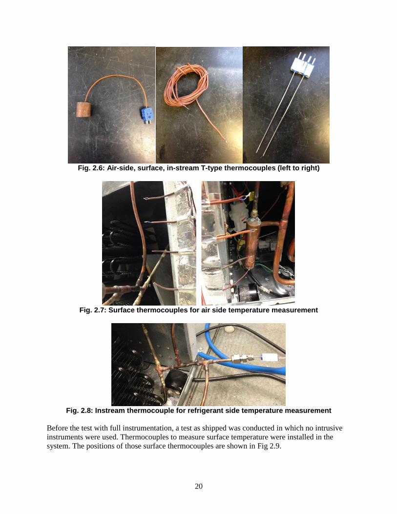
Considering the accuracy and the temperature range in the test, all thermocouples used in

the test were T-type thermocouples with 0.5°C accuracy. There were three different T-type

thermocouples used in the test to measure different temperature conditions (Fig. 2.6). The first

was the thermocouple used to measure refrigerator compartment temperatures. According to the

DOE standard, a cylindrical metallic mass 1.12 ± 0.25 inches (2.9 ± 0.6 cm) in diameter was

used to get stable temperatures in the compartments. The second was the surface thermocouple

installed on the surface of copper tubing on the refrigerant side. These were also used to measure

the air-side temperature at the inlet and outlet of the condenser (shown in Fig. 2.7). The third

type was an in-stream thermocouple. These were installed in the refrigerant side (shown in Fig.

2.8). In-stream thermocouples were placed at the midpoint of the copper tube to measure the

refrigerant temperature.

All of the air-side thermocouples and in-stream thermocouples were calibrated to reduce

the systematic uncertainty using a temperature calibrator. The calibration ranges were -20 to

36°C for air-side thermocouples and -20 to 50°C for in-stream thermocouples. The total

systematic uncertainty after calibration was 0.24°C.

20

Fig. 2.6: Air-side, surface, in-stream T-type thermocouples (left to right)

Fig. 2.7: Surface thermocouples for air side temperature measurement

Fig. 2.8: Instream thermocouple for refrigerant side temperature measurement

Before the test with full instrumentation, a test as shipped was conducted in which no intrusive

instruments were used. Thermocouples to measure surface temperature were installed in the

system. The positions of those surface thermocouples are shown in Fig 2.9.

21

Fig 2.9: Thermocouples installed in the system when testing as shipped

The thermocouples on the air-side in the fresh food and freezer compartments were located

according to the standard. The AHAM standard provides detailed position of thermocouples

according to different refrigerator inner structure. Fig. 2.10 shows the schematic based on our

testing unit. Fig. 2.11 shows pictures of the thermocouples positioned in the actual refrigerator.

Fig. 2.12 shows the positions of thermocouples measuring ambient temperature, one at each side

of the refrigerator.

Fig. 2.10: Locations of thermocouples measuring compartment temperature

1

77

2

3

4

5

6

Fresh Cabinet Freezer Cabinet

22

Fig. 2.11: Pictures of thermocouples in fresh food (left) and freezer (right) compartments

Fig. 2.12: Locations of thermocouples measuring ambient temperature (top-view (left);

side-view (right))

2.2.2.2 Pressure Transducers

Absolute pressure transducers were used in the test to get the pressure at the inlet of the

compressor and the outlet of the condenser. One of the Omega 0-250 psi strain type pressure

transducers is shown in Fig. 2.13. Also, Fig. 2.14 shows the differential pressure transducer used

to measure the pressure drop across the condenser.

23

Fig. 2.13: Pressure transducers used in the test

Fig. 2.14: Differential pressure transducer used to measure the condenser pressure drop.

2.2.2.3 Mass Flow Meter

Based on the estimated mass flow rate of 0.72g/s, a small Coriolis mass flow meter from

Micro Motion was used with an accuracy of 0.25% of reading. Fig. 2.15 shows the mass flow

meter and the transmitter. The mass flow meter was installed between compressor outlet and

condenser inlet to measure the vapor flow rate. The mass flow meter was installed upside down

so the vapor would not stick in the bottom of the curved tube in the mass flow meter.

24

Fig. 2.15: Mass flow meter and the transmitter (left to right)

The mass flow meter was calibrated in a range from 0.0 to 3.0 g/s using a linear fit and

coefficient of determination. R2 functions were set in Excel where a R

2 value of 99.99% was

established for this mass flow meter calibration data set.

2.2.2.4 Watt-hour Meter

The Watt-hour meter is simply a digit counter inside the watt meter. The watt meter used

in the test generates a pulse when 0.2 Wh of energy is consumed. At the end of each test, the

counter gave the precise energy consumption during the test. To validate the watt-hour meter,

two light bulbs were used. Since light bulb power consumption is quite stable, it was possible to

validate the watt-hour counter. Data was recorded for seven minutes, and the differences

between watt-hour counter and real energy consumed was within 0.1%.

2.3 Data Reduction The overall daily energy consumption of the unit was calculated according to the

Department of Energy standard. The refrigerator used in the test was a long-time automatic

defrost unit. Duration and energy consumption for both the stabilization and defrost cycles were

tested and recorded. The equation given by DOE standard is shown in Equation (1), the

calculation includes the energy consumption during steady state cycling as well as the defrost

cycle.

𝐸 = (1440×𝐸𝑃1

𝑇1) + (𝐸𝑃2 − (

𝐸𝑃1×𝑇2

𝑇1) × (

12

𝐶𝑇)) (1)

Where:

E= total energy consumption [kWh/day]

EP1= energy expended during the stabilization portion of the test [kWh]

T1 = duration of the stabilization portion of the test [min]

EP2 = energy expended in the defrost portion of the test [kWh]

T2 = duration of the defrost portion of the test [min]

CT = time between defrost cycles [min]

1440 = conversion factor to adjust to a 24-hour period in minutes per day

25

12 = factor to adjust for a 50-percent run time of compressor in hours per day

2.4 Uncertainty Analysis Table 2.2 shows the specifications of instruments that were used in the test and contains

the manufacturer, model number, measurement range, and systematic uncertainty of each

instrument. All of these instruments were connected to National Instruments field point modules,

and through LabVIEW software we could record data and calculate system performance

parameters in real time.

In general, to calculate the uncertainty in a measured variable, both systematic

uncertainty and random errors are considered. The systematic uncertainty is mainly the

uncertainty of the instruments. The random errors are taken as equal to the standard deviation of

the data used to calculate the average value. The total error is the sum of these two. However,

because random errors assess the deviation of test data from an average value, it is of

significance for steady state test data. For transient test data, there is no way to get an average, so

only systematic uncertainty was analyzed.

After collecting data, in order to calculate the systematic uncertainty of a calculated

variable, the systematic uncertainty of each measured variable used in the calculation must be

included. Equation (2) defines how to propagate these uncertainties to get the uncertainty of a

calculated value.

𝑢𝐹 = √(𝜕𝐹

𝜕𝑣1∗ 𝑢1)

2

+ (𝜕𝐹

𝜕𝑣2∗ 𝑢2)

2

+ ⋯ (𝜕𝐹

𝜕𝑣𝑖∗ 𝑢𝑖)

2

(2)

Where:

F = calculated variable

uF= uncertainty in the calculated variable “F”

ui= uncertainty of the measured variable

vi= measured variable

i = number of variables used to calculate “F”

Table 2.3 shows the systematic uncertainties calculated for the variables of interest in these tests.

Table 2.3: Calculation of systematic uncertainties

Variables Units Systematic uncertainty

Pressure kPa 8.62

Differential pressure kPa 0.17

In-steam temperature °C 0.44

Air-side temperature °C 0.24

Surface temperature °C 0.50

Mass flow rate g/s 0.0075

Total power consumption W 1

Per-day energy consumption Wh 0.001

26

3 SANDIA COOLER CONDENSER DEVELOPMENT

3.1 Conceptual Design

The general concept for the SCC was to use one or more impellers coupled with a baseplate that

would serve two functions: 1) provide the air bearing surface and motor stator mount for the

impeller(s) and 2) act as the refrigerant-side heat exchanger with fluid channels for refrigerant

flow. A shroud would be used to separate the inlet and exit air flow and direct the exit air toward

the compressor. The goal was to provide the same cooling capacity as the baseline condenser,

but in a more compact package due to the improved air-side heat exchange provided by the

Sandia Cooler. This goal was defined early in the project. An alternative goal could have been to

provide enhanced heat transfer performance in a similar size as the baseline condenser, but it was

thought that this approach might be more difficult to quantify.

The primary design requirements were thus the cooling capacity and the containment of the

refrigerant in channels or passages within or attached to the baseplate. These requirements were

subject to a number of constraints including refrigerant temperature and pressure, refrigerant

mass flow rate, allowable refrigerant pressure drop, and air inlet temperature. Values for these

parameters were taken initially from the refrigerator spec sheet and previous UMD refrigerator

testing data.

With the requirements and constraints defined, the design tasks included designing the baseplate,

sizing and designing the impellers, selecting the appropriate motor, shaft, bearings and

controller, designing a frame and shroud, and integrating these components into an overall

system design that could be easily assembled.

Initial impeller sizing calculations led to a decision to use two impellers in the 5-6” diameter

range. One large impeller could have been used, but the Sandia team was concerned with taking

a larger step in impeller diameter having previous experience only with 4” diameter designs.

With this decided, two concepts for the overall system configuration were developed and are

shown in Fig. 3.1 and Fig. 3.2. The side-by-side configuration would provide more space for the

refrigerant flow paths in the baseplate while the back-to-back configuration would be more

compact. Detailed refrigerant-side calculations were required to determine which configuration

to use.

27

Fig. 3.1: Side-by-side configuration

Fig. 3.2: Back-to-back configuration

The initial concept for the refrigerant channels was to use a micro-channel approach to provide

the high heat transfer coefficient that would be required for a compact baseplate. Commercially

available micro-channel extrusions would be attached to the bottom of the baseplate and

manifolded together as shown in Fig. 3.3 . This approach, however, was abandoned in favor of

an easier implementation: a spiral microchannel groove directly machined into the baseplate. The

new approach eliminated several possible issues that, if they were to arise, would be difficult to

solve with the limited time and budget. The issues eliminated included manifolds,

maldistribution of vapor and liquid, and an additional thermal interface. Fig. 3.4 shows the

concept.

28

Fig. 3.3: Initial refrigerant channel concept

Fig. 3.4: Spiral channel concept

To complete the baseplate design, heat transfer and pressure drop calculations for the spiral

channel were required. Also, this concept had to be incorporated into the physical layout of the

baseplate along with motor mount features and a fabrication process needed to be defined. Those

topics will be covered in the next sections.

3.2 Base Plate Design Fig. 3.5 shows the baseplate of the SCC. The baseplate physically serves as 1) the

stationary component on top of which the heat sink impeller rotates, and 2) the housing for

refrigerant channels. Per 1), the baseplate contributes to generating the hydrodynamic air-

bearing and also houses the stator of the motor driving the heat sink impeller. The baseplate

therefore plays a critical thermal role in transferring heat from the hot refrigerant to the heat sink

impeller, and was designed with the following considerations:

A) Low material usage

B) Tolerable pressure drop in the refrigerant flow

C) Sufficient heat transfer in the refrigerant flow

29

Fig. 3.5: Cross-sectional view of the baseplate. The inset shows the dimension

nomenclature for the channel geometry.

To address A), the footprint area of the baseplate was kept to a minimum. By orienting

the two impellers on opposing sides of the baseplate, the required baseplate footprint area was

approximately that of one impeller. Copper was chosen for the baseplate material for its high

thermal conductivity.

Regarding B), baseline tests were performed on the refrigerator with the original

equipment (OE) condenser to determine the pressure drop across the condenser. At a condenser

saturation temperature of 41°C, a 7.5-8 kPa pressure drop was measured. The effect of this

pressure change can be understood by referring to the local slope of the saturation curve at 41°C;

a 10 kPa difference in saturation pressure results in a corresponding difference of approximately

0.35°C change in the saturation temperature. Consequently, the 7.5-8 kPa pressure drop can be

interpreted to result in a negligibly small change in the condensation (saturation) temperature. In

this development, a 0.5°C shift in the condensation temperature was considered to be tolerable,

corresponding to an allowable pressure drop in the baseplate refrigerant channel of 10-15 kPa.

This temperature change was also approximately equal to the accuracy of the T-type

thermocouples used in experimentation.

Common heat transfer issues associated with parallel refrigerant channels (connected by

inlet and outlet manifolds/headers) is the distribution of the liquid and vapor phases, as well as

mass flow rates. Unfavorable distribution of liquid and vapor in parallel channels would result in

inefficient use of the channels for phase change heat transfer. Consequently, to avoid such

problems, a single refrigerant channel was employed. Furthermore, to mitigate the minor losses

from abrupt turns in the refrigerant flow, a spiral shaped channel was adopted, where the spiral

was inscribed within the footprint of the heat sink impeller.

Regarding B) and C), both pressure drop and heat transfer are strongly influenced by the

effective channel cross-sectional diameter (for a given temperature and mass flow rate) such that

decreasing the diameter has a detrimental effect on pressure drop (increase) and a beneficial

effect on heat transfer (increase). Selection of the appropriate effective diameter therefore needs

to balance the considerations of both B) and C). Furthermore, the overall channel length

determines the surface area available for heat transfer from the refrigerant to the channel walls,

and therefore also plays a critical role in influencing the heat transfer rate and temperature of the

condenser. The following subsections describe the heat transfer (Section 3.2.1) and pressure

drop (Section 3.2.2) analyses performed to determine the appropriate effective channel diameter

and length for a set of operating conditions. To match the performance of the original condenser,

these conditions were taken to be the condenser temperatures and mass flow rate measured in the

baseline experiment with the original condenser at the medium setting (for details see Section

W H

T

30

4.1)) The operating conditions and final channel dimensions are listed in Table 3.1and Table 3.5

below, respectively.

. Table 3.1: Operating conditions used to design the baseplate refrigerant channel

geometry.

Condition Units Values

Ambient temperature °C 32.2

Condenser inlet temperature °C 75

Condenser (saturation) temperature °C 41

Condenser exit temperature °C 40

Mass flow rate g/s 1

Table 3.2: Dimensions of the baseplate refrigerant channel geometry, as shown in Fig. 3.5. The channel length is the outer length of the spiral.

Dimension Units Values

Channel height (H) mm 2.54

Channel width (W) mm 2.54

Thickness of channel wall (T) mm 1.42

Channel length m 4.00

3.2.1 Heat Transfer Analysis The total heat transferred is a function of the overall heat transfer coefficient, heat

transfer area and temperature difference between the refrigerant and air.

Q = UA ∙ ∆T (3)

In Equation (3), Q stands for total heat transferred, U is the overall heat transfer coefficient of the

condenser, A is the heat transfer area, and ∆T is the temperature difference between the two

fluids. ∆T is often taken as the Log Mean Temperature Difference (LMTD), but Mean

Temperature Difference is used here to simplify the calculation. In the condenser, heat is

transferred from the high temperature refrigerant through convection to the wall of the

refrigerant channels, then the heat is conducted through the metal wall to the air-side surfaces,

finally, the heat is convectively transferred to the ambient air. From this perspective, the total

heat transfer can be defined from the point of view of thermal resistance:

Q =∆𝑇

∑ 𝑅𝑖

(4)

where the thermal resistance for the SCC is:

31

∑ 𝑅𝑖 =1

ℎ𝑟𝑒𝑓𝐴𝑟𝑒𝑓+

𝑑𝑤

𝑘𝑐𝑜𝑝𝑝𝑒𝑟𝐴𝑤+ 𝑅𝑎𝑖𝑟𝑠𝑖𝑑𝑒.

(5)

Here ℎ𝑟𝑒𝑓 is the heat transfer coefficient on the refrigerant-side, 𝐴𝑟𝑒𝑓 is the refrigerant-side area,

dw is the wall thickness, kcopper is the thermal conductivity of the copper plate, and Aw is the cross

section area of the copper wall. The air-side thermal resistance is that of the Sandia Cooler

impellers plus the air gap between the impellers and the baseplate.

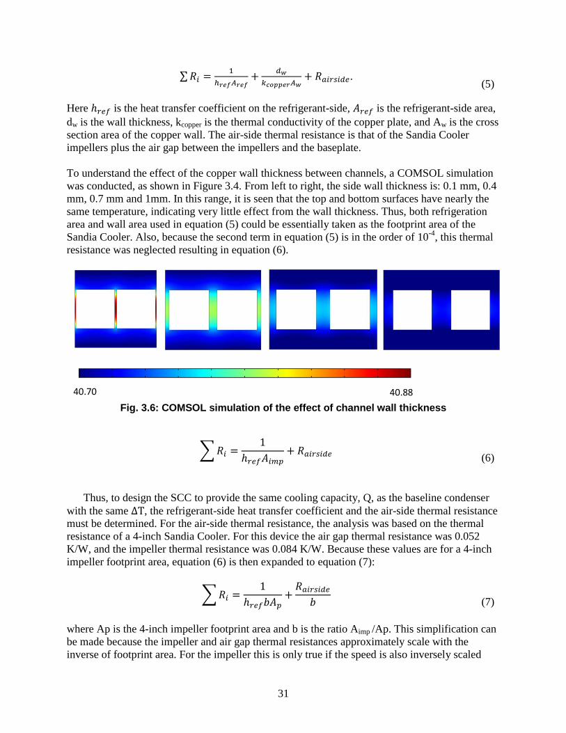
To understand the effect of the copper wall thickness between channels, a COMSOL simulation

was conducted, as shown in Figure 3.4. From left to right, the side wall thickness is: 0.1 mm, 0.4

mm, 0.7 mm and 1mm. In this range, it is seen that the top and bottom surfaces have nearly the

same temperature, indicating very little effect from the wall thickness. Thus, both refrigeration

area and wall area used in equation (5) could be essentially taken as the footprint area of the

Sandia Cooler. Also, because the second term in equation (5) is in the order of 10-4

, this thermal

resistance was neglected resulting in equation (6).

Fig. 3.6: COMSOL simulation of the effect of channel wall thickness

∑ 𝑅𝑖 =1

ℎ𝑟𝑒𝑓𝐴𝑖𝑚𝑝+ 𝑅𝑎𝑖𝑟𝑠𝑖𝑑𝑒

(6)

Thus, to design the SCC to provide the same cooling capacity, Q, as the baseline condenser

with the same ∆T, the refrigerant-side heat transfer coefficient and the air-side thermal resistance

must be determined. For the air-side thermal resistance, the analysis was based on the thermal

resistance of a 4-inch Sandia Cooler. For this device the air gap thermal resistance was 0.052

K/W, and the impeller thermal resistance was 0.084 K/W. Because these values are for a 4-inch

impeller footprint area, equation (6) is then expanded to equation (7):

∑ 𝑅𝑖 =1

ℎ𝑟𝑒𝑓𝑏𝐴𝑝+

𝑅𝑎𝑖𝑟𝑠𝑖𝑑𝑒

𝑏

(7)

where Ap is the 4-inch impeller footprint area and b is the ratio Aimp /Ap. This simplification can

be made because the impeller and air gap thermal resistances approximately scale with the

inverse of footprint area. For the impeller this is only true if the speed is also inversely scaled

40.70 40.88

32

with diameter. Thus, an 8-inch diameter impeller operating at 1250 rpm has a thermal resistance

that is ~4 times lower than a 4-inch diameter impeller operating at 2500 rpm.

The key parameter to decide then was the refrigeration-side heat transfer coefficient. This

coefficient is largely dependent on a hydraulic diameter, tube configuration, refrigerant type,

fluid phase, and Reynolds number.

For single phase flow, the correlation is well developed under a wide range of operating

conditions, but for two-phase flow it is not. Therefore, a number of correlations were

investigated. For simplification, several assumptions for heat transfer and pressure drop

calculations were made as follows:

Although the channel was spiral in the baseplate, it was assumed to be straight.

Because of the spiral shape, there was a temperature gradient along the radial direction

resulting in radial heat transfer. However, this channel to channel heat transfer was

neglected.

The spiral channel causes some secondary flow due to centrifugal force. This would

increase the heat transfer coefficient and increase pressure drop compared to a straight

channel. However, the effect of centrifugal force was neglected.

After literature review, three correlations for refrigeration side heat transfer coefficient

were selected, Wang et al (2002), Shah (2009) and Koyama et al (2002) [7,8,9]. These

correlations were compared with the experiment result by Yan and Lin (1998) [17] as shown in

Fig. 3.7. Data and model predictions are shown for a mass flow rate of 200 kg/ (m2·s), a

hydraulic diameter of 2 mm, a saturation temperature of 30°C and a heat transfer rate of 10

kW/m2. From the comparison, it was found that Shah’s correlation under-predicted the results,

while Koyama’s correlation slightly over-predicted experiment results with a similar trend.

Wang’s correlation agreed with experiment data at the point when the quality is 0.5, while under

predicting the result in the high quality region. Since it is difficult to know the quality change

inside the channel, an average quality of 0.5 was taken to calculate the heat transfer coefficient.

From this point of view, Wang’s correlation was closest to the experimental data and thus was

used for the analysis.

33

Fig. 3.7: Comparison of different heat transfer coefficient correlation with experiment

data for R134a

Based on Wang’s correlation, in two-phase flow regimes there exists a combined annular

and stratified flow effect. For low mass flux flow, the flow is more likely to form stratified flow,

in which the heat transfer in the bottom pool is small compared to the film-wise condensation in

the top portion. In our case, because the mass flow rate for the refrigerant is around 1 g/s, the

flow will more likely be in the stratified flow regime. Therefore, the following correlation was

used to calculate the Nusselt number.

𝑁𝑢𝑠𝑡𝑟𝑎𝑡 =∝ 𝑁𝑢𝑓𝑖𝑙𝑚 + (1−∝)𝑁𝑢𝑐𝑜𝑛𝑣𝑒𝑐𝑡𝑖𝑜𝑛 (8)

∝= (1 +1 − 𝑥

𝑥(

𝜌𝑣

𝜌𝑙)

23

)−1

(9)

𝑁𝑢𝑓𝑖𝑙𝑚 = 0.555(𝜌𝑙(𝜌𝑙 − 𝜌𝑣)𝑔ℎ𝑓𝑔𝐷ℎ

3

𝑘𝑙𝜇𝑙(𝑇𝑠𝑎𝑡 − 𝑇𝑤))1/4

(10)

𝑁𝑢𝑐𝑜𝑛𝑣𝑒𝑐𝑡𝑖𝑜𝑛 = 0.023𝑅𝑒𝑙0.8𝑃𝑟𝑙

0.4

(11)

There are three dimensionless numbers in the correlation: the Nusselt number gives the

effect of convective heat transfer compared to conductive heat transfer and is a function of the

Reynolds number which describes the turbulence of the flow and the Prandtl number which is

defined as the ratio of momentum diffusivity to thermal diffusivity:

Re =𝜌𝑣𝐷ℎ

𝜇

(12)

0

1

2

3

4

5

6

0 0.2 0.4 0.6 0.8 1

He

at T

ran

sfe

r C

oe

ffic

ien

t [k

W/(

m2 *

K]

Quality [-]

EXP Shah [2009]

W-Wang [2002] Koyama [2002]

34

Nu =ℎ𝐷ℎ

𝑘

(13)

Pr =𝑐𝑝𝜇

𝑘

(14)

Thus, the heat transfer coefficient for the refrigerant-side was calculated from Equation (13).

Table 3.3 shows the refrigerant-side heat transfer analysis.

Table 3.3: Refrigeration-side heat transfer analysis for baseplate design

Heat Transfer Analysis Phase Unit Values

Refrigeration side heat transfer coefficient Vapor W/m2·K 511.4

Two-

phase

W/m2·K 2735.8

Liquid W/m2·K 386.3

Total Heat transfer area Vapor m2 0.0043

Two-

phase

m2 0.0264

Liquid m2 0.0007

Heat transferred Vapor W 36.7

Two-

phase

W 162.0

Liquid W 1.5

Total heat transferred W 200

As the table shows, the two-phase region has the highest heat transfer coefficient. However, the

cooling capacity for the two-phase region is also larger than that for the single phase regions.

The table shows that out of the 200 W of total heat, the two-phase region accounts for 162 W.

When we sum the heat transfer area together, it is 0.0314 m2. Referring back to equation (7), this

gives b = 3.99. So, the analysis indicated that the area of approximately four 4-inch impellers

was needed. This area is slightly larger (~6%) than the footprint area of two 5.5-inch impellers. It

was also determined from this analysis that the back-to-back configuration (Fig. 3.2) could

provide the refrigerant-side heat transfer area required. Due to the compactness of that

configuration, that was the design that was carried forward.

3.2.2 Pressure Drop Analysis Eight correlations for the two-phase pressure drop were selected: a homogenous model,

Lockhart-Martinelli (1949)[10], Mishima (1996), Lee (2001) [13], Chen (2001) [12], Sun (2009)

[11], Li (2010) [14] and Zhang (2010) [16]. Nino’s experimental data [15] was used to compare

these correlations. Fig. 3.8 shows the comparison of different correlations.

35

Fig. 3.8: Comparison of different pressure drop correlation with experiment data for

R134a

It is shown that most of the correlations under predicted the experiment data. An average quality

of 0.5 was used in the pressure drop analysis. Lockhart-Martinelli’s correlation shows the best

results and it was chosen for the analysis. The correlation is as follows:

(𝑑𝑃

𝑑𝑙)𝑇𝑃 = ∅𝑙

2(𝑑𝑃

𝑑𝑙)𝑙

(15)

The coefficient Ф provides an equivalent liquid pressure drop. This coefficient Ф is defined as:

∅𝑙2 = 1 +

𝐶

𝑋+

1

𝑋2 (16)

𝐶 = 12

(17)

𝑋2 =(𝑑𝑃𝑑𝑙

)𝑙

(𝑑𝑃𝑑𝑙

)𝑣

(18)

(𝑑𝑃

𝑑𝑙)𝑙 = 𝑓𝑙

2𝑚2(1 − 𝑥)2

𝐷ℎ𝜌𝑙

(19)

(𝑑𝑃

𝑑𝑙)𝑣 = 𝑓𝑣

2𝑚2𝑥2

𝐷ℎ𝜌𝑣

(20)

0

2

4

6

8

10

12

14

16

18

20

0 0.2 0.4 0.6 0.8 1

Pre

ssu

re D

rop

[kP

a/m

]

Quality [-]

EXP data

L-M [1949]

Mishima [1996]

Lee [2001]

Chen [2001]

Sun [2009]

Li [2010]

Zhang [2010]

Homogenous

36

In the correlation, 𝑓𝑙 and 𝑓𝑣 are Fanning friction factor. Using this correlation, a refrigerant-side

pressure drop analysis was carried out based on the channel dimensions arrived at through the

heat transfer analysis. The results of the pressure drop analysis are shown in Table 3.4.

Table 3.4: Refrigeration side heat transfer analysis for baseplate design

Pressure Drop Analysis Phase Unit Values

Refrigeration side pressure drop

per meter

Vapor kPa 2.40

Two-phase kPa 2.67

Liquid kPa 0.14

Channel length

Vapor m 0.61

Two-phase m 3.73

Liquid m 0.09

Pressure drop

Vapor kPa 1.46

Two-phase kPa 9.95

Liquid kPa 0.01

Total pressure drop kPa 11.42

In the table above, the channel length is calculated under the condition that side wall thickness is

1.0 mm. The length is calculated as:

𝐿 =𝐴

𝑑 + 𝑑𝑠𝑤 (21)

Where A is the area from Table 3.3, d is the channel width of 2.54 mm, and dsw is the side wall

thickness. When summing all the lengths together, the total length is 4.43 m. Thus, the pressure

drop for 1 g/s refrigerant flow through this channel should be close to 11.4 kPa which is in the

acceptable range.

As mentioned previously, the pressure drop was calculated based on the assumption that the

channel was straight. However, considering the small radius for the inside channel, the effect of

centrifugal force on the secondary flow could be non-negligible.

3.2.3 Base Plate Fabrication Fig. 3.9 shows that the copper baseplate consists of a main plate and a planar lid. The

refrigerant channel was milled into the main plate, and later closed by brazing the lid to the main

plate. All other features, including the peripheral mounting tabs, grooves for the air bearing, and

holes for wire and fluid delivery, were machined after the brazing was complete. These features

are labeled in Fig. 3.10 and Fig. 3.11, which show the assembled baseplate. The planar surfaces

of the baseplate were lapped to provide a flat interface to the heat sink impeller. Refrigerant

delivery tubes (OD=4.76 mm, ID=3.25 mm) were soldered onto the baseplate for a hermetic

connection.

37

Fig. 3.9: Components of the baseplate: the main plate and lid. All channel features are

machined into the main plate. The machined channel is closed by brazing the main plate and lid together

Fig. 3.10: Top-view of the completed baseplate

Refrigerant

Inlet/outlet

lines

Groove for air-

bearing

Mounts for

enclosure

Mounting for

motor stator

38

Fig. 3.11: Access ports in the baseplate

3.3 Impeller Design and Fabrication

The first step in the impeller design was to determine the size based on the requirements and

constraints. An initial analysis based on a set of preliminary requirements pointed to a two-

impeller design with 5-6” diameter impellers. A more detailed analysis was undertaken once the

baseline tests of the actual refrigerator were carried out. Calculations for both the air-side and

refrigerant-side were carried out to determine the impeller footprint that would be required to

meet the cooling capacity of the baseline condenser. The result of these calculations was that two

5.5” diameter impellers would provide the required footprint and air-side heat transfer.

The fin geometry for the impellers would be a scaled version of the 4” V5 impeller that was

developed by Sandia for electronics cooling. This impeller had 80 fins that were 0.030” thick and

0.095” tall. Scaled, the fins would be 0.041” thick and 1.31” tall.

The two 5.5” diameter impellers were fabricated at SNL using a Haas OM-2A CNC vertical 4-

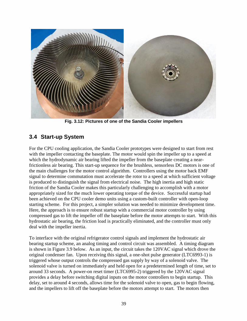
axis mill with a 30,000rpm spindle. Fig. 3.12 shows pictures of one impeller. The picture on the

left shows the impeller fins and the preload nut and spring used to set the air bearing height. The

picture on the right shows the rotor magnets, flux ring, and bearing attached to the base of the

impeller. The bearing, observed in both pictures, was pressed into an interference fit in the

platen. The figure also shows the anti-friction coating on the base of the impeller. This

graphite/MoS2 coating was also used in the original Sandia Cooler design to enable startup and

prevent wear and galling between the impeller and baseplate surfaces. As will be discussed in the

next section, the coating wasn’t used for startup in this prototype.

Compressed

gas ports

Motor

wire ports Thermocouple port

39

Fig. 3.12: Pictures of one of the Sandia Cooler impellers

3.4 Start-up System

For the CPU cooling application, the Sandia Cooler prototypes were designed to start from rest

with the impeller contacting the baseplate. The motor would spin the impeller up to a speed at

which the hydrodynamic air bearing lifted the impeller from the baseplate creating a near-

frictionless air bearing. This start-up sequence for the brushless, sensorless DC motors is one of

the main challenges for the motor control algorithm. Controllers using the motor back EMF

signal to determine commutation must accelerate the rotor to a speed at which sufficient voltage

is produced to distinguish the signal from electrical noise. The high inertia and high static

friction of the Sandia Cooler makes this particularly challenging to accomplish with a motor

appropriately sized for the much lower operating torque of the device. Successful startup had

been achieved on the CPU cooler demo units using a custom-built controller with open-loop

starting scheme. For this project, a simpler solution was needed to minimize development time.

Here, the approach is to ensure robust startup with a commercial motor controller by using

compressed gas to lift the impeller off the baseplate before the motor attempts to start. With this

hydrostatic air bearing, the friction load is practically eliminated, and the controller must only

deal with the impeller inertia.

To interface with the original refrigerator control signals and implement the hydrostatic air

bearing startup scheme, an analog timing and control circuit was assembled. A timing diagram

is shown in Figure 3.9 below. As an input, the circuit takes the 120VAC signal which drove the

original condenser fan. Upon receiving this signal, a one-shot pulse generator (LTC6993-1) is

triggered whose output controls the compressed gas supply by way of a solenoid valve. The

solenoid valve is turned on immediately and held open for a predetermined length of time, set to

around 33 seconds. A power-on reset timer (LTC6995-2) triggered by the 120VAC signal

provides a delay before switching digital inputs on the motor controllers to begin startup. This

delay, set to around 4 seconds, allows time for the solenoid valve to open, gas to begin flowing,

and the impellers to lift off the baseplate before the motors attempt to start. The motors then

40

accelerate to a speed sufficient for the hydrodynamic air bearings to lift the impellers before the

solenoid valve is closed. For shutdown, when the 120VAC condenser fan signal is removed,

power is removed from the power-on reset timer, and the digital inputs on the motor controllers

immediately go low. As the impellers decelerate, the air bearing gaps close until the impellers

touch down and come to rest on the baseplate. The anti-wear, anti-friction coating applied to the

impellers prevents galling between the two surfaces.

Fig. 3.13: Timing diagram for start-up

3.5 Motor and Controller

3.5.1 Motor Selection

The SCC uses two small brushless DC (BLDC) outrunner motors much like the Motrolfly

assembly shown in Fig. 3.14. They are comprised of 1) an iron core stator with copper windings,

2) NdFeB rare earth magnets and 3) a flux ring. The magnets and flux ring are bonded to the

rotor/impeller. The impeller thus rotates around the fixed stator. BLDC motors were chosen over

other motors primarily because of their reliability, compact size, high efficiency, high torque and

low noise characteristics.

41

Fig. 3.14: Motrolfly motor assembly

The condenser prototype utilizes custom wound 3 phase-WYE connected, brushless, sensor-less

DC motors. The stator, which is mounted directly to the baseplate, has 12 stator teeth wound in

a DLRK (Distributed - Lucas, Retzbach and Kühfuss) configuration, which is shown in Fig.

3.15. The three phases are represented in red, blue and green, with “S” and “E” signifying start

and end of the phase windings respectively. The three ends (E1, E2 and E3) are all tied together

to form the neutral, while the starts (S1, S2, S3) are connected to the motor controller driver.

The rotor (impeller) contains 14 NdFeB rare earth magnets. This arrangement provides an

electronic gear ratio of 7:1, thus providing more torque at the required rpm range and a more

precise 8.57 degrees of movement per step to reduce cogging. The DLRK winding technique

requires less copper windings per stator tooth, which is a critical factor due to space constraints

of this compact design. To reduce the footprint and cost even further, no rotor position sensors

(hall effect) are used and a sensor-less control technique is therefore required to control motor

commutation.

Fig. 3.15: DLRK Winding

It is important to specify a motor that is capable of producing the continuous required torque at

the rated speed as well as intermittent periods of high torque to overcome rotor inertia. In order

to get a motor that produces the required amount of torque while maintaining high efficiency and

a small footprint, it is necessary to look at several parameters. The speed/torque curve shown in

Fig. 3.16 demonstrates that a motor will produce a large amount of torque intermittently at

S1

E3

S2E1

S3

E2

NEUTRAL

42

startup and as the speed increases, the amount of torque output will decrease. Ideally, continuous

operation should occur between the rated torque and rated speed limits.

Fig. 3.16: Torque-speed curve

Torque is directly related to the magnetic flux, the diameter and height of the stator, the number

of windings, and the current drive from the controller. For the Sandia Cooler, a small diameter

stator was desired to maximize the surface area for heat transfer between the baseplate and

impeller. In addition, a shorter stator would also reduce the thickness of the baseplate. Thus, the

smallest motor possible was chosen that could still deliver the required torque. Once the size of

the motor is selected, the correct wire size and number of turns per phase must be determined.

With small diameter stators, large gauge wire cannot be used and therefore smaller gauge wire

with a larger turn count is required. With increasing turns of smaller gauge wire comes a higher

phase resistance and back EMF constant (Ke). The back EMF constant represents the voltage

that is produced by the motor rotating at a specific rpm. As the motor speeds up, the increasing

back EMF reduces the voltage to drive current through the windings. If the windings aren’t

chosen correctly, the current available and thus torque available to drive the motor at a given

speed is significantly reduced.

After careful analysis and comparison of other available motors, a Motrolfly DM2205 motor was

selected to provide the required torque at the highest efficiency. The DM2205 is a standard off-

the-shelf component that is commonly used in the hobby arena. It has a stator dimension of 22

mm in diameter and is nominally 6 mm in height. Initial selection of this motor was based on

torque data acquired from a 4 inch V5 impeller used on the Sandia Cooler. For the 4” impeller,

10.5 mN-m of torque is required to maintain a constant speed of 2000 rpm. The condenser

impeller, which utilizes the same V5 design but has an increased diameter of 5.5 inches, requires

approximately 2.6 times more torque to maintain the same rotational speed. The theoretical

value of 27 mN-m at 2000 rpm (2.6 x 10.5 mN-m) was therefore used as the minimum motor

torque requirement for this prototype.

From previous experimental data, it is known that a DM2203 motor with 85 turns of 34 AWG

magnet wire yields a motor speed constant Kv = 800 rpm/volt. This speed constant can then be

used to derive the theoretical torque at a given current drive as follows:

Kt = 9554/Kv (mN-m/A)

Kt = 9554/800

= 11.94 mN-m/A,

Speed

Torque

Max

Peak

RatedTorque

Con nuousTorque

RatedSpeed

Speed/torquerela on

Intermi entTorque

43

where Kt is the motor torque constant.

Based on these numbers, the DM2203 motor produces about half of the required torque that the

condenser impeller requires. While maintaining the same gauge wire and number of turns, and

magnetic properties, doubling the stator height roughly halves the motor speed constant KV to

about 400 rpm/volt, which doubles the torque constant. The theoretical torque produced by a

DM2205 motor would therefore be approximately twice that of the DM2203, which is close to

the calculated torque required for the larger 5.5” impeller.

A bare 2205 stator was wound with 85 turns of 34 AWG wire and placed in a setup to measure

the motor speed constant Kv. The resulting experimental value for Kv was found to be roughly

half (390 mv/rpm) that of the DM 2203. To prove that the DM2205 motor was capable of

producing the necessary torque at the given speed, it was placed on a Placid industries H11-24-1

hysteresis brake similar to the setup shown in Fig. 3.17 below. Torque data was taken using an

Allied Motion 30V/10Amp DPFlex BLDC motor controller and can be seen in Table 3.5, Fig.

3.18, and Fig. 3.19 below.

Fig. 3.17: Hysteresis Brake setup

Torque and efficiency evaluation tests were made at a fixed speed of 2000 rpm with a supply

voltage of 25V. The goal was to determine the maximum torque output at the projected

experimental speed. The test consisted of using a bench top 25V supply to power the DPFlex

controller at a nominal 2000 rpm. The hysteresis brake was commanded to provide a brake

torque sweep from 0 to 50 mN-m. A maximum torque value of 48.89 mN-m was found by

gradually increasing the brake torque until the motor began to slow and chatter. The motor was

shown to provide approximately 80% more maximum torque than theoretically required by the

impeller. Therefore, the supply voltage was reduced to better match the back EMF of the motor

and reduce switching losses to increase overall efficiency. It should be noted that the DPFlex

controller consumes about 2.5W of idle power and that all efficiency calculations include this

44

power loss. It was determined that at a target torque of 30 mN-m and 2000 rpm, the minimum

supply voltage is 20VDC. Power consumption at 20VDC was noted to be 10.4 W, as compared

to 11 W at 25 VDC. While this lower supply voltage provides a 5% increase in efficiency, it

could compromise the ability of the impeller to overcome the rotor inertia and start successfully

100% of the time. It was therefore decided that 25VDC provided the best efficiency with the

most reliable startup.

Table 3.5: DM2205-390 Brake torque test at 2000 rpm and Vsupply = 25V

speed (rpm)

brake torque (mNm)

mechanical power out (W)

Electrical power (W) Efficiency

2012.57 0.00 0.00 0.96 0.00

2012.57 1.31 0.28 1.08 0.25

2010.86 2.67 0.56 1.46 0.38

2009.14 7.42 1.56 2.89 0.54

2016.86 18.16 3.84 6.44 0.60

2012.57 30.14 6.35 11.00 0.58

2005.71 36.84 7.74 13.95 0.55

2016.86 48.89 10.33 21.11 0.49

Fig. 3.18: Torque output vs. power consumption at 2000 rpm with 25V supply

0.00

5.00

10.00

15.00

20.00

25.00

30.00

35.00

40.00

45.00

50.00

0.00 5.00 10.00 15.00 20.00 25.00

Torq

ue

ou

tpu

t (m

Nm

)

Electrical Power (W)

Torque vs Electrical Power @ rpm DPflex controller and Custom Motrolfly DM-2205-390

45

Fig. 3.19: Electrical to mechanical efficiency vs. torque output at 2000 rpm with 25 V

supply

3.5.2 Controller Selection

For initial testing of the Sandia cooler, an inexpensive off the shelf hobby motor controller was

used to drive the motor. These controllers are typically used for radio controlled planes and cars

and use a very simple square wave pulse width modulated drive signal and typically provide a

low startup torque. Later a more sophisticated controller, the Allied Motion DPFlex control

modules were used that rely on trapezoidal commutation using pulse width modulation. Both

methods generate torque ripple, which can introduce audible noise into the system; however for

this prototype the added noise introduced by this type of controller was not a concern.

The DPflex controller was used extensively throughout the course of the development of the

Sandia Cooler prototype and as a result the experience gained allowed for a straightforward

implementation into the condenser prototype. A 30V/10A version was selected over the 16 Volt

version, after it was shown that a minimum of 20 volts was required to generate sufficient torque

for the impeller to rotate at 2000 rpm.

3.5.3 Control Module

After selecting the appropriate motor controller for driving the stators, it was necessary to

package the controllers in a control box. The control box contains a controller for each impeller,

a 25 V DC power supply, the timing and control circuitry for triggering the air solenoid and

starting the motors, a front panel potentiometer tuned to set the speed, LEDs for status and a

LCD panel for power consumption readout. Fig. 3.20 below shows the front panel and rear

0.00

0.10

0.20

0.30

0.40

0.50

0.60

0.70

0.00 10.00 20.00 30.00 40.00 50.00 60.00

ele

ctri

cal t

o m

ech

anic

al e

ffic

ien

cy

torque output (mNm)

Efficiency at 2000 rpm DPflex controller and Custom Motrolfly DM-2205-390

46

panel of the control box. Compressed air or N2 (35-45 psig) is fed into the box via a quick

disconnect fitting on the back of the unit, which is then fed to the control solenoid valve. This

valve, which opens upon receiving an AC trigger from the refrigerator, allows air to flow to the

air ports on the front panel and into the baseplate for the static air bearing during startup.

To ensure smooth operation and accurate speed control of the impellers, slight modifications to

the PID loops and other settings was required after setting the final air gap height. A final supply

voltage of 24 VDC was found to provide the smoothest and most efficient operation. The

DPflex controller has a wide variety of parameters to tune and there are a few key settings that

are required. Firstly, the starting current maximum was set to 1.20 amps. This value provided

the best startup without hesitation or jitter. Current settings too high generate unstable startup

and overheat the motor windings and conversely, settings too low will not start the motor at all.

The controller has an inner and an outer control loop and parameters for these were set. Other

settings included reducing the ping period and increasing the timeout. The ping period specifies

the pulse width of current pulses to each phase of the stator, while the timeout controls the

duration of the ping cycle during startup. This rotating ping approach is necessary to overcome

the inertia of the rotor during startup. Once the impeller is brought up to a speed where an

adequate back EMF signal can be used to determine rotor position and speed, the controller will

go into closed loop speed control.

Fig. 3.20: Front/Rear panel

The block diagram shown in Fig. 3.21 shows the general electrical layout of the controller box.

Standard 120VAC/60Hz power is provided to an adjustable 25 VDC switching power supply.

This power supply provides parallel power to two 30V DPflex controllers and the control PCB.

The power supplied to both DPflex controllers is monitored using a Medusa Research Power

Analyzer Pro meter placed in series. Speed control is achieved through a resistive voltage

MotorControllerlayout

FilteredSupplyAir/N2@35-40psig

120VACtrigger

PowerMeter

MainPower

Gasforstartupairbearing

3Phasepowertomotors

Manualmotordisable

47

divider potentiometer with an analog display, which is linearly calibrated to rotational speed.

Both controllers receive the same control signal and maintain speeds within 1% of each other as

verified using a strobe light. Both impellers are enabled/disabled using AC input from the

refrigerator, which is converted on the control PCB to a 0V (OFF) and 24V (ON) signal. The

operator can manually disable the motors via a toggle switch located on the front panel. Fuses

protect the general circuitry from potential shorts and overcurrent situations. Each DPflex

controller has also been programmed with a maximum current of 3 amps in the event of a stall

condition to prevent damage to the stators.

Fig. 3.21: Controller Block Diagram

3.6 Shroud Design A volute-style shroud was incorporated around the heat sink impellers to deliver a

concentrated exhaust air flow to the compressor for cooling. In designing the shroud, emphasis

was placed on the ease of fabrication; commercially available 7” (17.8 cm) diameter acrylic

tubing was used for the curved portion of the housing, and laser-cut sheet-stock aluminum was

used for the planar end housings (Fig. 3.22). Metal mesh was attached to the end housings to

prevent debris from entering the Sandia Cooler intake. Fasteners were used to clamp the planar

end housings to the baseplate, fixing the acrylic portion in place. The total height (in the axial

direction) of the condenser assembly was 12.4 cm; the total occupied volume was approximately

3.5 L.

25VDC

PowerMeter

Toimpeller1motor

Toimpeller2motor

DPflexcontroller

DPflexcontroller

ControlPCB

ACTrigger

AirSolenoid

SpeedControl

Airsupply

Toimpeller1Airbearing

Toimpeller2Airbearing

ACSupply

Enable/Disable

SpeedCNTL

48

Fig. 3.22: Exploded view of main shroud components

3.7 Final Assembly

Fig. 3.23 shows a CAD image of the fully assembled SCC and Fig. 3.24 shows a cross-section.

In the cross-section view, the motor assemblies can be seen which take up the central portion of

the baseplate and impellers. Note that the primary reason for the thickness of the baseplate was

to accommodate the motor stators and shafts. This was done for simplicity for this prototype

unit. The baseplate thickness would be substantially reduced in a commercial design to minimize

weight and cost.

1. Sheet metal outer

housing (two pieces

clamp in place mesh

filter)

2. Acrylic shroud for

volute

3. Stand-offs

4. Baseplate

5. Mounting studs

6. Sheet metal plate

for volute exit

49

Fig. 3.23: SCC assembly

Fig. 3.24: Cross-section of the SCC assembly

To assemble the SCC, the first step was to integrate the motor assemblies with the baseplate.

Fig. 3.25 shows an image of one of the stator/shaft assemblies attached to the baseplate. The

wires for the motor were fed through radial holes in the baseplate and connectors attached. The

next step was to integrate the impellers and set the air bearing gap. Fig. 3.26 shows one impeller

mounted to the baseplate. The nut that is used to set the air bearing gap can be seen attached to

the shaft in the center of the impeller.

Baseplate

Heat Sink

Impellers

50

Fig. 3.25: Motor stator and shaft assembled to the baseplate

Fig. 3.26: One impeller mounted to the baseplate

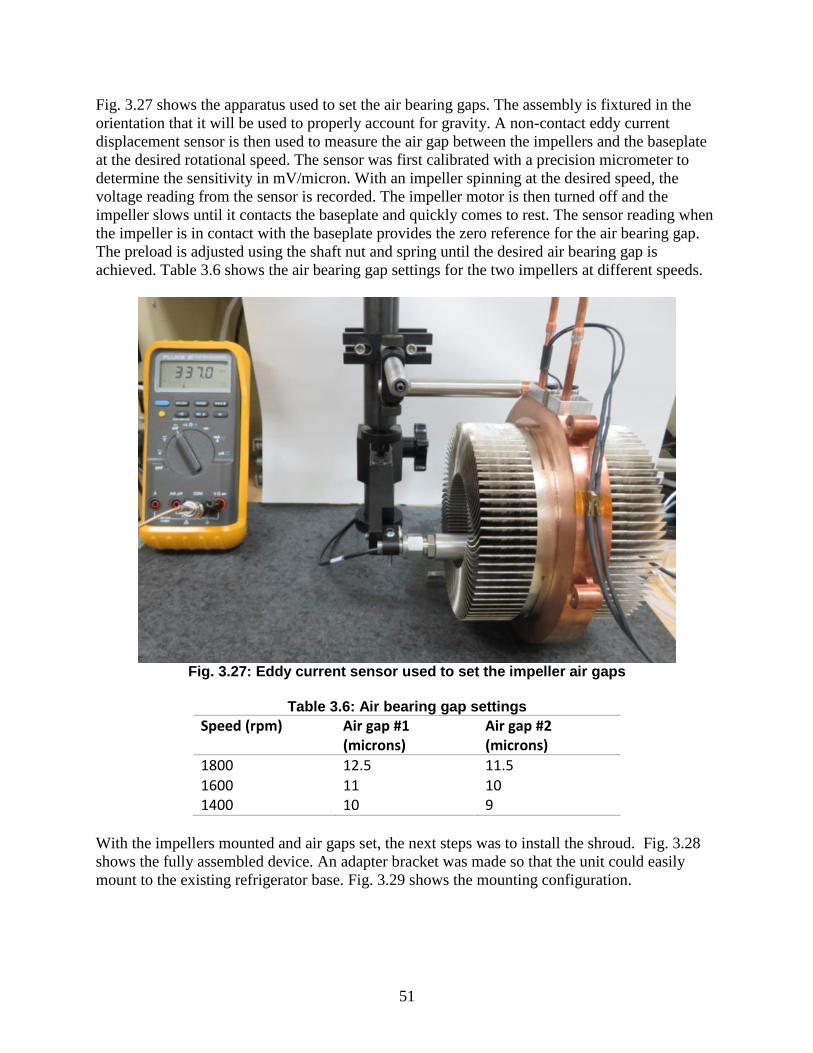
51

Fig. 3.27 shows the apparatus used to set the air bearing gaps. The assembly is fixtured in the

orientation that it will be used to properly account for gravity. A non-contact eddy current

displacement sensor is then used to measure the air gap between the impellers and the baseplate

at the desired rotational speed. The sensor was first calibrated with a precision micrometer to

determine the sensitivity in mV/micron. With an impeller spinning at the desired speed, the

voltage reading from the sensor is recorded. The impeller motor is then turned off and the

impeller slows until it contacts the baseplate and quickly comes to rest. The sensor reading when

the impeller is in contact with the baseplate provides the zero reference for the air bearing gap.

The preload is adjusted using the shaft nut and spring until the desired air bearing gap is

achieved. Table 3.6 shows the air bearing gap settings for the two impellers at different speeds.

Fig. 3.27: Eddy current sensor used to set the impeller air gaps

Table 3.6: Air bearing gap settings

Speed (rpm) Air gap #1 (microns)

Air gap #2 (microns)

1800 12.5 11.5

1600 11 10 1400 10 9

With the impellers mounted and air gaps set, the next steps was to install the shroud. Fig. 3.28

shows the fully assembled device. An adapter bracket was made so that the unit could easily

mount to the existing refrigerator base. Fig. 3.29 shows the mounting configuration.

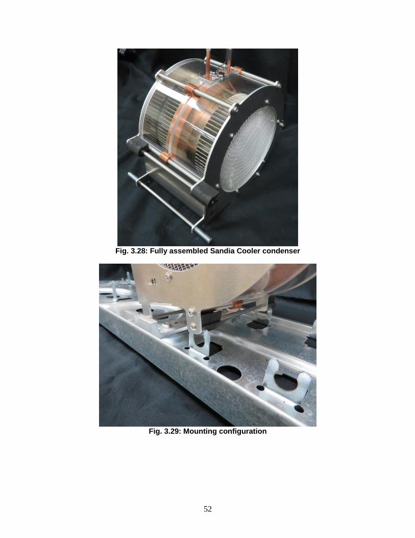
52

Fig. 3.28: Fully assembled Sandia Cooler condenser

Fig. 3.29: Mounting configuration

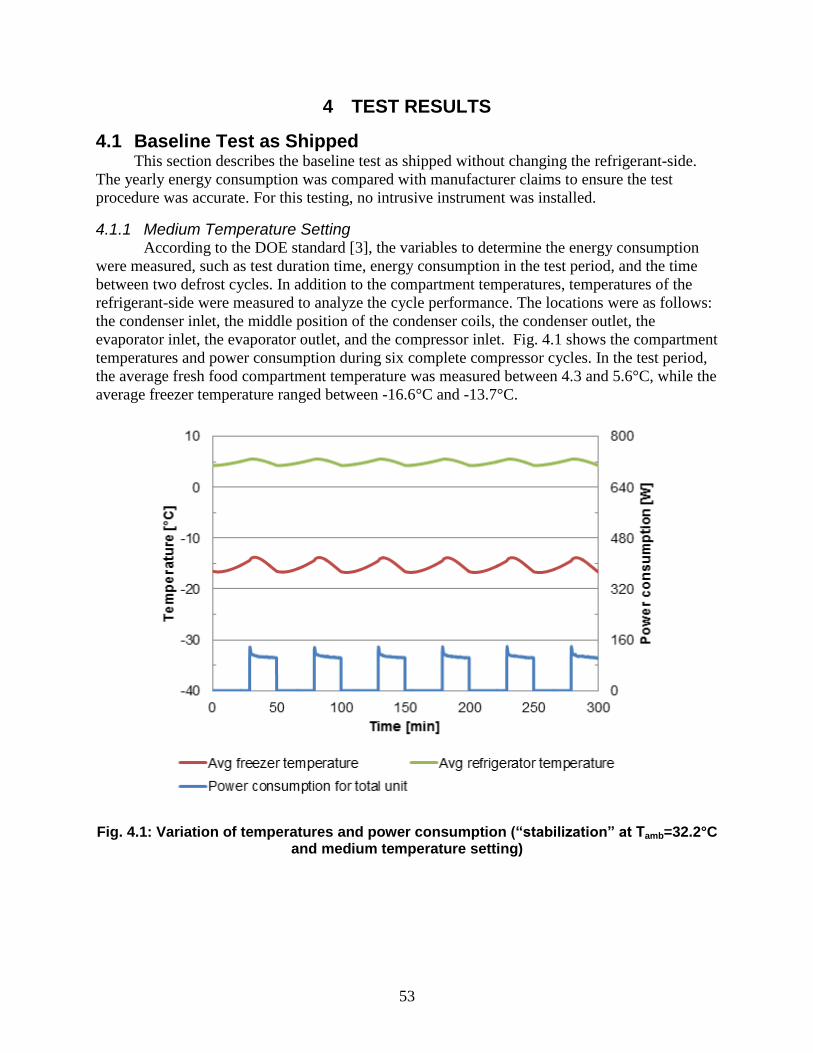
53

4 TEST RESULTS

4.1 Baseline Test as Shipped This section describes the baseline test as shipped without changing the refrigerant-side.

The yearly energy consumption was compared with manufacturer claims to ensure the test

procedure was accurate. For this testing, no intrusive instrument was installed.

4.1.1 Medium Temperature Setting According to the DOE standard [3], the variables to determine the energy consumption

were measured, such as test duration time, energy consumption in the test period, and the time

between two defrost cycles. In addition to the compartment temperatures, temperatures of the

refrigerant-side were measured to analyze the cycle performance. The locations were as follows:

the condenser inlet, the middle position of the condenser coils, the condenser outlet, the

evaporator inlet, the evaporator outlet, and the compressor inlet. Fig. 4.1 shows the compartment

temperatures and power consumption during six complete compressor cycles. In the test period,

the average fresh food compartment temperature was measured between 4.3 and 5.6°C, while the

average freezer temperature ranged between -16.6°C and -13.7°C.

Fig. 4.1: Variation of temperatures and power consumption (“stabilization” at Tamb=32.2°C and medium temperature setting)

54

Fig. 4.2: Variation of surface temperatures on refrigerant-side (“stabilization” at Tamb=32.2°C and medium temperature setting)

Fig. 4.2 shows the temperatures on the refrigerant-side. When the compressor is on, the

temperatures at the compressor and condenser increase to a quasi-stable point. When the

compressor is turned off the temperatures drop quickly to near ambient. At the evaporator, the

reverse trend is seen.

Fig 4.3: Variation of temperatures and power consumption (“defrost” at Tamb=32.2°C and medium temperature setting)

55

Fig 4.3 shows the air-side temperatures and power consumption changes during the defrost cycle

at the medium temperature setting. There was a “precool” step before the defrost heater turned

on. When the heater was turned on, the power increased up to 300 W, lasting about 10 minutes.

During this period, the compartment temperatures increased continuously, with the freezer

temperature reaching 0 C before the recovery cycle starts. The air-side temperature change in the

fresh food compartment was much smaller than that in the freezer. A long recovery cycle is then

needed to bring back the temperatures to the normal range.

Fig 4.4: Variation of surface temperatures on refrigeration-side (“defrost” at Tamb=32.2°C and medium temperature setting)

Temperatures on the refrigerant-side are shown in Fig 4.4. When the defrost heater is turned on,

the temperature of the evaporator increases up to 35°C then slowly drops as the frost melts. It

then takes nearly 50 minutes for the evaporator temperatures to recover.

For the stabilization test , six complete compressor on/off cycles were recorded and detailed

temperature values are shown in Table 4.1 and Table 4.2. The temperature at the compressor

outlet shows the highest value of 74.2°C. These values were used in the design of the baseplate

of the SCC.

Table 4.1: Air-side data at medium temperature setting

Variables Units Stabilization Defrost Uncertainty

Ambient temp. °C 32.3 32.3 0.24

Average fresh food air temp. °C 4.9 5.6 0.24

56

Average freezer air temp. °C -15.5 -11.6 0.24

Compressor on time min 125.7 55.0 -

Compressor off time min 174.4 87.0 -

Energy consumption kWh 0.2288 0.1264 0.0002

Table 4.2: Refrigerant temperature at medium temperature setting

Variables Units Stabilization Defrost Uncertainty

Compressor discharge temp. °C 74.2 76.1 0.5

Condenser middle temp. °C 40.3 41.0 0.5

Condenser outlet temp. °C 41.1 41.7 0.5

4.1.2 Warmest Temperature Setting

From the air side temperature data in Table 4.1, the average compartment temperatures in

the stabilization period were 4.9°C (fresh food compartment) and -15.5°C (freezer). Both of

these temperatures were lower than the standard temperatures, which are 7.2°C (fresh food

compartment) and -15.0°C (freezer), respectively. So, the following test was conducted at the

warmest temperature setting. Fig. 4.5 to Fig. 4.8 show temperatures for the air-side and

refrigerant-side for both the stabilization period and the defrost cycle period.

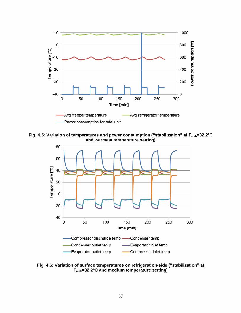
57

Fig. 4.5: Variation of temperatures and power consumption (“stabilization” at Tamb=32.2°C and warmest temperature setting)

Fig. 4.6: Variation of surface temperatures on refrigeration-side (“stabilization” at Tamb=32.2°C and medium temperature setting)

58

Fig. 4.7: Variation of temperatures and power consumption (“defrost” at Tamb=32.2°C and warmest temperature setting)

Fig. 4.8: Variation of surface temperatures on refrigeration-side (“defrost” at Tamb=32.2°C and medium temperature setting)

59

Fig. 4.5 to Fig. 4.8 show the same data as Fig. 4.1 to Fig 4.4 for the stabilization and defrost

cycles. Average fresh food compartment temperature and freezer temperature during

stabilization cycles were 8.6°C and -11.1°C, which were both higher than the medium

temperature setting(4.9°C and -15.5°C). Temperature values for the warmest temperature setting

are shown in Table 4.3 and Table 4.4. The air-side temperatures were higher than that at the

medium temperature setting. On the refrigerant-side, the temperatures did not change much.

Under the medium temperature setting, the total time for the stabilization cycle and defrost cycle

was longer than for the warmest temperature setting. This is because the cooling load for the

medium temperature setting was larger than the warmest temperature setting. When calculating

the yearly energy consumption under both temperature settings, the equation in section 2.3 is

used based on the DOE standard [3].

Table 4.5 summarizes the compartment temperatures and energy usage for the two settings. The

energy consumption values were 370.6 kWh for the warmest temperature setting and 446.5 kWh

for the medium temperature setting. 370.6 kWh was used as the final estimated yearly energy

consumption for this unit. Compared with the manufacturer’s yearly energy consumption of 383

kWh, the test result was within 4%, showing a good match with the manufacturer’s data.

Table 4.3: Air side specifications of test data at warmest temperature setting

Variables Units Stabilization Defrost Uncertainty

Ambient temp. °C 32.3 32.3 0.24

Average fresh food air temp. °C 8.6 9.1 0.24

Average freezer air temp. °C -11.1 -7.2 0.24

Comp. on time min 91.1 41.5 -

Comp. off time min 177.3 87.3 -

Energy consumption kWh 0.1700 0.1040 0.0002

Table 4.4: Condenser related surface temperature at warmest temperature setting

Variables Units Stabilization Defrost Uncertainty

Compressor discharge temp. °C 74.1 76.7 0.5

Condenser middle temp. °C 41.0 41.3 0.5

Condenser outlet temp. °C 41.9 42.2 0.5

60

Table 4.5: Summary of test data in “test as shipped”

Refrigerator Settings Medium Warmest

Variables Units Stabilization

Defrost cycle

Uncertainty Stabilizat

ion Defrost

cycle Uncertainty

Ambient temp. °C 32.3 32.3 0.24 32.3 32.5 0.24

Avg. freezer temp.

°C -15.5 -11.6 0.24 -11.1 -7.2 0.24

Avg. fresh food temp.

°C 4.9 5.6 0.24 8.6 9.1 0.24

Energy consumption

kWh 0.2288 0.1264 0.0002 0.1700 0.1040 0.0002

Duration time min 300.1 142.0 - 268.4 128.8 -

Daily energy consumption

kWh 1.22 0.001 1.02 0.001

Yearly energy consumption

kWh 446.5 0.36 370.6 0.40

4.2 Baseline Test with Full Instrumentation Compared to the baseline test as shipped, the three surface thermocouples were replaced by

in-stream T-type thermocouples to measure temperature at the condenser inlet, the condenser

outlet, and the compressor outlet. Two pressure transducers were installed measuring pressure at

the condenser outlet and compressor inlet. One differential pressure transducer was installed to

measure pressure drop across the condenser. Fig. 4.9 shows a schematic diagram of the

measurement points of the system. Fig. 4.10 shows how the instruments were installed.

61

Fig. 4.9: Schematic diagram of the system

4.2.1 Refrigerant Charge Optimization

The refrigerant charge was varied to have the same performance as achieved from the

“test as shipped”. Average freezer compartment temperature, average fresh food compartment

temperature, compressor on time and compressor off time in one complete cycle were measured.

All the charge optimization tests were conducted at the medium temperature setting.

As shown in Table 4.6, as the charge amount was increased, the average freezer

compartment temperature approached that from the test as shipped, while the average fresh food

compartment temperature did not change much. Considering that the fresh food compartment

temperature was controlled by a damper, it was not as sensitive to the refrigerant amount under

Condenser

Evaporator

MFM

TT

T

T

T

Hot Pipe

Capillary Tube

T-Thermocouple

P-Pressure Transducer

DP-Differential Pressure Transducer

MFM-Mass Flow Meter

SLHX-Suction Line Heat Exchanger

P

DP

T

SLHX

P

1

4

3 2

5

6

1

6 5

4

2

3

Mass flow meter

To pressure transducer

To differential pressure transducer

Fig. 4.10: Instruments installed in the experiment set up

62

given ranges. Compressor on time of the current test increased as compared to that of the “test as

shipped”. When the refrigerant charge amount was 121.6 g, the average freezer temperature and

compressor off time was similar to the baseline. Therefore, 121.6 g was chosen as the optimized

charging amount for the test with full instrumentation.

Table 4.6: Charging optimization for a complete cycle

Mass of charged R134a [g]

Avg. freezer temp. [°C]

Avg. fresh food cabinet temp. [°C]

Comp. on time [min]

Comp. off time [min]

Test as shipped -15.5 4.9 20.9 29

96.2 -13.4 4.5 28.2 28.8

102.2 -14.0 4.5 26.2 28.6

111 -15.0 4.5 23.7 29.0

121.6 -15.6 4.5 23.0 29.1

122.6 -15.3 4.6 22.6 28.4

Data shown in Table 4.7 are the average values during one compressor-on time. When the

compressor turned on, the mass flow rate increased rapidly during the first several seconds and

then gradually reduced. Generally, a higher refrigerant charge would increase the evaporator and

condenser capacities of the system. When the mass of R134a was charged from 96.2 g to 122.6

g, the average mass flow rate increased from 0.79 g/s to 0.94 g/s. The condenser pressure drop

decreased from 11.0 kPa to 9.9 kPa as the refrigerant charge was increased. With the varying

charges, average subcooling of the system was almost zero if considering the measurement

uncertainty. Average superheating decreased slightly with increasing mass charged.

Table 4.7: Charging optimization for one compressor-on time

Mass of charged

R134a [g]

Avg. mass flow rate

[g/s]

Avg. condenser pressure drop

[kPa]

Avg. superheat

[K]

Avg. subcool

[K]

Inlet air temp.

[°C]

Outlet air temp.

[°C]

96.2 0.79 11.0 - - 32.5 36.2

102.2 0.83 11.3 56.3 0.02 32.3 36.3

111 0.90 11.7 55.6 0.03 32.5 36.4

121.6 0.94 10.9 55.4 0.02 32.6 36.6

122.6 0.93 9.9 51.9 1.20 32.6 36.6

4.2.2 Medium Temperature Setting Results Following the charge optimization, testing was conducted with the same procedure as

before to estimate yearly energy consumption. Compared to the previous test, more information

about mass flow rate and pressure are presented in this section. In Fig. 4.11, similar trends were

shown for average cabinet temperature and power consumption for the total unit. Six complete

cycles were analyzed for the stabilization part. The red line indicates that average freezer

temperature cycled between -16.6°C and -13.5°C while average temperature of the fresh food

compartment ranged between 4.1°C to 5.4°C. When compared to the temperatures in the DOE

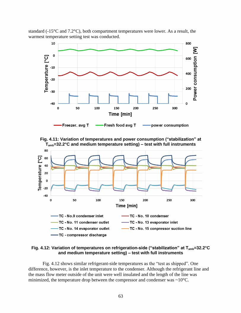
63

standard (-15°C and 7.2°C), both compartment temperatures were lower. As a result, the

warmest temperature setting test was conducted.

Fig. 4.11: Variation of temperatures and power consumption (“stabilization” at Tamb=32.2°C and medium temperature setting) – test with full instruments

Fig. 4.12: Variation of temperatures on refrigeration-side (“stabilization” at Tamb=32.2°C and medium temperature setting) – test with full instruments

Fig. 4.12 shows similar refrigerant-side temperatures as the “test as shipped”. One

difference, however, is the inlet temperature to the condenser. Although the refrigerant line and

the mass flow meter outside of the unit were well insulated and the length of the line was

minimized, the temperature drop between the compressor and condenser was ~10°C.

64

Fig. 4.13 Variation of pressure and pressure drop (“stabilization” at Tamb=32.2°C and medium temperature setting)

Fig. 4.13 shows the compressor discharge and suction pressures, and the pressure drop across the

condenser. When the compressor was on, discharge pressure was about 1,070 kPa and suction

pressure was about 100 kPa. The refrigerant pressure drop across the condenser was measured at

about 9 kPa.

Mass flow rate is an important parameter in designing the baseplate for the SCC. Fig.

4.14 shows the changes of mass flow rate in the system during the medium temperature tests.

The maximum value went to 1.98 g/s for several seconds, then rapidly dropped to 0.9 g/s and

gradually decreased. The average mass flow rate for compressor-on time was 0.93 g/s. In one

complete cycle, the compressor on-time was around 22.7 min and the time that the mass flow

rate was higher than 1 g/s was 2.7 min. Thus, the assumption of 1 g/s was reasonable for the

design calculations.

Compressor

65

Fig. 4.14 Variation of mass flow rate (“stabilization” at Tamb=32.2°C and medium temperature setting)

Fig. 4.15 Variation of condenser sub-cool and suction line superheat (“stabilization” at Tamb=32.2°C and medium temperature setting)

Degrees of superheat and subcool are defined as below:

𝑇𝑠𝑢𝑝𝑒𝑟ℎ𝑒𝑎𝑡 = 𝑇𝑐𝑜𝑚𝑝.in − 𝑇𝑠𝑎𝑡𝑝.𝑐𝑜𝑚𝑝.𝑖𝑛 (23)

𝑇𝑠𝑢𝑏𝑐𝑜𝑜𝑙 = 𝑇𝑠𝑎𝑡𝑝.𝑐𝑜𝑛𝑑.𝑜𝑢𝑡 − 𝑇𝑐𝑜𝑛𝑑.𝑜𝑢𝑡 (24)

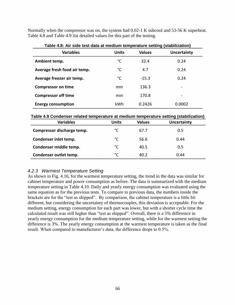
66

Normally when the compressor was on, the system had 0.02-1 K subcool and 53-56 K superheat.

Table 4.8 and Table 4.9 list detailed values for this part of the testing.

Table 4.8: Air side test data at medium temperature setting (stabilization)

Variables Units Values Uncertainty

Ambient temp. °C 32.4 0.24

Average fresh food air temp. °C 4.7 0.24

Average freezer air temp. °C -15.3 0.24

Compressor on time min 136.3 -

Compressor off time min 170.8 -

Energy consumption kWh 0.2426 0.0002

Table 4.9 Condenser related temperature at medium temperature setting (stabilization)

Variables Units Values Uncertainty

Compressor discharge temp. °C 67.7 0.5

Condenser inlet temp. °C 56.6 0.44

Condenser middle temp. °C 40.5 0.5

Condenser outlet temp. °C 40.2 0.44

4.2.3 Warmest Temperature Setting As shown in Fig. 4.16, for the warmest temperature setting, the trend in the data was similar for

cabinet temperature and power consumption as before. The data is summarized with the medium

temperature setting in Table 4.10. Daily and yearly energy consumption was evaluated using the

same equation as for the previous tests. To compare to previous data, the numbers inside the

brackets are for the “test as shipped”. By comparison, the cabinet temperature is a little bit

different, but considering the uncertainty of thermocouples, this deviation is acceptable. For the

medium setting, energy consumption for each part was lower, but with a shorter cycle time the

calculated result was still higher than “test as shipped”. Overall, there is a 5% difference in

yearly energy consumption for the medium temperature setting, while for the warmest setting the

difference is 3%. The yearly energy consumption at the warmest temperature is taken as the final

result. When compared to manufacturer’s data, the difference drops to 0.5%.

67

Fig. 4.16: Variation of temperatures and power consumption (“stabilization” at Tamb=32.2°C and warmest temperature setting)

‘ Table 4.10: Summary of test data in “Test with full instruments”

Refrigerator Settings Medium Warmest

Variables Units Stabilizatio

n Defrost

cycle Uncertainty

Stabilization

Defrost cycle

Uncertainty

Ambient temp. °C 32.4 (32.3) 32.5

(32.3) 0.24

32.4 (32.3)

32.4 (32.5)

0.24

Avg. freezer temp.

°C -15.3

(-15.5) -11.8

(-11.6) 0.24

-10.8 (-11.1)

-7.2 (-7.2)

0.24

Avg. fresh food temp.

°C 4.7 (4.9) 5.0 (5.6) 0.24 8.7 (8.6) 9.3 (9.1) 0.24

Energy consumption

kWh 0.2426

(0.2288) 0.1436

(0.1264) 0.0002

0.1750 (0.1700)

0.1010 (0.1040)

0.0002

Duration time min 307.1

(300.1) 150.0

(142.0) -

267.0 (268.4)

127.9 (128.8)

-

68

Daily energy consumption

kWh 1.28 (1.22) 0.001 1.04 (1.02) 0.001

Yearly energy consumption

kWh 467.2 (446.5) 0.35 381.1 (370.6) 0.40

4.2.4 Testing Repeatability In order to make sure the test result was reliable; part of the test was repeated. Table 4.11 shows

the result just for the stabilization part at the medium temperature setting. Six cycles were used

as before, and as the table shows, while both energy consumed and duration are different in each

test, the final result is within 2% for the three trials.

Table 4.11: Result of repeat test (stabilization at medium temperature setting)

Times 1st

2nd

3rd

EP1 [kWh] 0.2426 0.2464 0.2434

T1 [min] 307.10 307.08 303.32

EP2 [kWh] 0.1436 0.1400 0.1458

T2 [min] 150.02 148.18 149.58

CT [min] 1269 1207 1366

Per-day energy consumed[kWh] 1.28 1.29 1.30

Per-year energy consumed[kWh] 467.2 472.4 474.6

Deviation compared to 1st

[%] 0 1.1 1.6

4.3 Sandia Cooler Condenser Test

Fig. 4.17 shows the initial configuration for the SCC installed in the refrigerator. However, this

layout resulted in poor airflow to the rear impeller. The flow rate to the rear impeller was lower

than that of the front impeller due to the configuration. Moreover, the exiting air from the SCC

recirculated to the rear impeller. This recirculation of hot air increased the air inlet temperature

reducing the performance of the unit. To overcome this issue, the configuration was modified.

The whole unit was taken out of the refrigerator as shown in Fig. 4.18. A separator was installed

between the condenser and the refrigerator to block the backflow to the Sandia Cooler inlet. This

configuration provided better airflow for optimum performance.

69

Fig. 4.17: Scheme #1: SCC in the refrigerator unit

Fig. 4.18: Scheme #2: SCC out of the refrigerator unit

Table 4.12 shows the comparison for the airside conditions for scheme #1 and scheme #2. For

the SCC, the rpm was set to 1400 for both conditions. The ambient temperature was set to

32.2 °C for all the tests. When the SCC was located in the refrigerator unit, the impeller inlet air

temperature was higher than that in baseline test, especially for the rear side, which was 3 K

higher. When the unit was moved out, airside conditions for the SCC improved significantly.

Averaged inlet air temperature was comparable with the baseline.

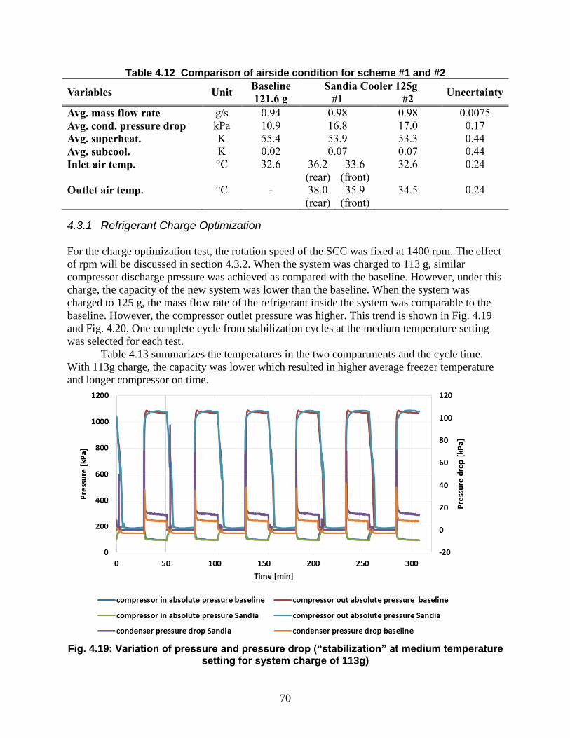
70

Table 4.12 Comparison of airside condition for scheme #1 and #2

Variables Unit Baseline

121.6 g

Sandia Cooler 125g Uncertainty

#1 #2

Avg. mass flow rate g/s 0.94 0.98 0.98 0.0075

Avg. cond. pressure drop kPa 10.9 16.8 17.0 0.17

Avg. superheat. K 55.4 53.9 53.3 0.44

Avg. subcool. K 0.02 0.07 0.07 0.44

Inlet air temp. °C 32.6 36.2

(rear)

33.6

(front)

32.6 0.24

Outlet air temp. °C - 38.0

(rear)

35.9

(front)

34.5 0.24

4.3.1 Refrigerant Charge Optimization

For the charge optimization test, the rotation speed of the SCC was fixed at 1400 rpm. The effect

of rpm will be discussed in section 4.3.2. When the system was charged to 113 g, similar

compressor discharge pressure was achieved as compared with the baseline. However, under this

charge, the capacity of the new system was lower than the baseline. When the system was

charged to 125 g, the mass flow rate of the refrigerant inside the system was comparable to the

baseline. However, the compressor outlet pressure was higher. This trend is shown in Fig. 4.19

and Fig. 4.20. One complete cycle from stabilization cycles at the medium temperature setting

was selected for each test.

Table 4.13 summarizes the temperatures in the two compartments and the cycle time.

With 113g charge, the capacity was lower which resulted in higher average freezer temperature

and longer compressor on time.

Fig. 4.19: Variation of pressure and pressure drop (“stabilization” at medium temperature

setting for system charge of 113g)

71

Fig. 4.20: Variation of pressure and pressure drop (“stabilization” at medium temperature

setting for system charge of 125g)

Table 4.13: Cabinet temperatures and cycle time comparison (Stabilization at medium

temperature setting, rpm is fixed at 1400)

Variables Unit Baseline

121.6 g

Sandia Cooler Uncertainty

113 g 125 g

Avg. freezer temp. °C -15.6 -15.0 -15.5 0.24

Avg. fresh food temp. °C 4.5 4.8 4.9 0.24

Avg. superheat. K 55.4 55.2 53.3 0.44

Avg. subcool. K 0.02 0.1 0.07 0.44

Comp. on time min 23.0 23.3 21.6 -

Comp. off time min 29.1 27.8 28.1 -

The energy consumption of the refrigerator unit was investigated with the SCC under different

charges. Six stabilization cycles were selected at the medium temperature setting. The total

energy consumption is divided into two parts. One part is the energy consumed by the vapor

compression cycle; the other part is the fan or impeller power consumption. For the baseline test,

the fan power consumption during the compressor on time was 4 W. For the SCC, the power

consumption for the impeller was 12 W at 1400 rpm and 27 W at 1800 rpm. The total time for

the six stabilization cycles varied due to the test conditions. So it was unfair to simply compare

the total energy consumption. Average power consumption for an hour is also given in Table

4.14.

72

Table 4.14: Energy consumption of different charges for six stabilization cycles (medium temperature setting, rpm is fixed at 1400)

Variables Unit Baseline

121.6 g

Sandia Cooler Uncertainty

113 g 125 g

VCC consumption kWh 0.2334 0.247 0.231 0.0002

Fan consumption kWh 0.0092 0.0355 0.0310 0.0002

Total energy consumption kWh 0.2426 0.2825 0.262 0.0002

Time min 307.1 307.9 297.2 -

Averaged VCC consumption W 45.6 48.1 46.6 0.04

Averaged total consumption W 47.4 55.1 51.9 0.04

For the SCC with the 125 g refrigerant charge, the vapor compression cycle average energy

consumption is nearly identical to the baseline system. A difference of just 2.3% is seen between

the two values. Note that this is close to the difference seen between repeated tests with the

baseline system. This result verifies the condenser design which was developed to match the

performance of the baseline unit. Thus, the 125 g charge was taken as the condition to use for

further comparison.

Note that the SCC is able to provide this performance in a significantly smaller volume.

However, when accounting for the fan/impeller energy consumption, the average total energy

consumption for the SCC is 9.5% higher than the baseline. This is due to the fact that the

baseline condenser fan only consumes 4 W during operation while the Sandia Cooler

motor/controller system consumes 12 W at 1400 rpm.

Since the refrigeration cycle is transient, instead of using the average values for the whole

process, it is more reliable to analyze a specific instantaneous point. The moment when the

compressor stops at the end of the on-time period was selected for further analysis between the

different configurations. Table 4.15 shows the detailed values.

Table 4.15: Properties of optimized charge (instantaneous values before the compressor

turns off, medium temperature setting, rpm is fixed at 1400)

Variables Unit Baseline

121.6 g

Sandia Cooler

125 g Uncertainty

Comp. suction pressure kPa 94.6 95.5 8.62

Comp. discharge pressure kPa 1,065.1 1,095.5 8.62

Pressure ratio - 11.3 11.5 -

Comp. suction density kg/m3 4.0 3.9 0.36

Condenser outlet pressure kPa 1,057.2 1,080.8 8.62

Mass flow rate g/s 0.85 0.85 0.0075

Comp. suction temperature °C 28.4 30.1 0.44

Comp. discharge temperature °C 56.6 55.3 0.44

Condenser outlet temperature °C 40.2 42.1 0.44

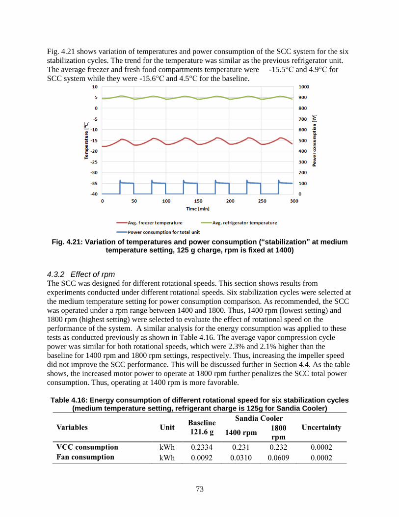
73

Fig. 4.21 shows variation of temperatures and power consumption of the SCC system for the six

stabilization cycles. The trend for the temperature was similar as the previous refrigerator unit.

The average freezer and fresh food compartments temperature were -15.5°C and 4.9°C for

SCC system while they were -15.6°C and 4.5°C for the baseline.

Fig. 4.21: Variation of temperatures and power consumption (“stabilization” at medium

temperature setting, 125 g charge, rpm is fixed at 1400)

4.3.2 Effect of rpm The SCC was designed for different rotational speeds. This section shows results from

experiments conducted under different rotational speeds. Six stabilization cycles were selected at

the medium temperature setting for power consumption comparison. As recommended, the SCC

was operated under a rpm range between 1400 and 1800. Thus, 1400 rpm (lowest setting) and

1800 rpm (highest setting) were selected to evaluate the effect of rotational speed on the

performance of the system. A similar analysis for the energy consumption was applied to these

tests as conducted previously as shown in Table 4.16. The average vapor compression cycle

power was similar for both rotational speeds, which were 2.3% and 2.1% higher than the

baseline for 1400 rpm and 1800 rpm settings, respectively. Thus, increasing the impeller speed

did not improve the SCC performance. This will be discussed further in Section 4.4. As the table

shows, the increased motor power to operate at 1800 rpm further penalizes the SCC total power

consumption. Thus, operating at 1400 rpm is more favorable.

Table 4.16: Energy consumption of different rotational speed for six stabilization cycles

(medium temperature setting, refrigerant charge is 125g for Sandia Cooler)

Variables Unit Baseline

121.6 g

Sandia Cooler

Uncertainty 1400 rpm

1800

rpm

VCC consumption kWh 0.2334 0.231 0.232 0.0002

Fan consumption kWh 0.0092 0.0310 0.0609 0.0002

74

Total energy consumption kWh 0.2426 0.262 0.293 0.0002

Time min 307.1 297.2 299.1 -

Averaged VCC

consumption W 45.6 46.6 46.5 0.04

Averaged total

consumption W 47.4 51.9 58.8 0.04

As before, the point when the compressor stopped was selected for properties analysis. Table

4.17 summarizes the performance of the SCC under different rotational speeds. The pressures

and temperatures for the two speeds are very close. It can be concluded that the rotational speed

for the SCC doesn’t significantly influence the system performance over this speed range.

Table 4.17: Properties of different rotational speed (instantaneous values before the

compressor turns off, medium temperature setting, 125g charge for Sandia Cooler tests)

Variables Unit Baseline

121.6 g

Sandia Cooler

Uncertainty 1400

rpm

1800

rpm

Comp. suction pressure kPa 94.6 95.5 94.8 8.62

Condenser outlet pressure kPa 1057.2 1080.8 1084.8 8.62

Comp. discharge pressure kPa 1065.1 1095.5 1099.0 8.62

Cond. Pressure drop kPa 7.9 14.7 14.2 0.17

Pressure ratio - 11.2 11.5 11.6 -

Comp. suction density kg/m3 4.0 3.9 3.9 0.36

Mass flow rate g/s 0.85 0.85 0.84 0.0075

Comp. suction temperature °C 28.4 30.1 30.2 0.44

Comp. discharge temperature °C 56.6 55.3 54.2 0.44

Condenser outlet temperature °C 40.2 42.1 42.3 0.44

Note: instantaneous values before the compressor turns off, medium temperature setting,

refrigerant charge is 125g for SCC.

4.4 Discussion

4.4.1 Predicted vs. Measured Performance

4.4.1.1 Air-side heat transfer

The air-side heat transfer performance for the SCC can be easily calculated based on measured

and calculated quantities from the experimental results. If the thermal resistance is taken as

follows:

𝑅𝑎𝑖𝑟𝑠𝑖𝑑𝑒 =(𝑇𝑏𝑎𝑠𝑒𝑝𝑙𝑎𝑡𝑒 − 𝑇𝑎𝑖𝑟)

𝑄 (25)

75

where Rairside refers to the summation of impeller thermal resistance and air gap thermal

resistance, then just two temperatures and the heat transfer rate are needed. In the experiments,

the air inlet temperature to the condenser was measured by several thermocouples and the values

averaged. The condenser baseplate temperature was measured by one thermocouple positioned in

a thermocouple well that was about 1-inch deep. Based on the discussion in Section 3.2, the

baseplate can be assumed to be essentially isothermal. Thus, this single temperature

measurement should be indicative of the overall baseplate temperature.

The heat transfer rate, Q, from the baseplate to the ambient air has two components. The first

component is the heat removed from the refrigerant. As shown in equation (26), this component

was calculated using the refrigerant mass flow rate �̇� and the change in enthalpy from the inlet

to the outlet of the condenser. The total heat dissipated by the SCC also includes a component

from the impeller motors as shown in equation (27). At 1400 rpm, the motor power is 12 W and

at 1800 rpm it is 27 W. Approximately 50% of this power is dissipated as heat.

𝑸𝒄𝒐𝒏𝒅 = �̇� × (𝒉𝒄𝒐𝒏𝒅 𝒊𝒏 − 𝒉𝒄𝒐𝒏𝒅 𝒐𝒖𝒕) (26)

𝑸 = 𝑸𝐜𝐨𝐧𝐝 + 𝑸𝒎𝒐𝒕𝒐𝒓 × 𝟓𝟎% (27)

Table 4.18 shows the air-side thermal resistance calculated using equations (25)-(27) for both the

1400 rpm and 1800 rpm SCC data. The values represent the average over the six stabilization

cycles for each test.

Table 4.18: Measured air-side thermal resistance

Parameters Unit Sandia Cooler

1400 rpm 1800 rpm

Mass flow rate g/s 0.95 0.94

Qcond W 164.6 161.0

Impeller power W 12.0 27.0

Total heat Q W 170.6 174.5

Airside inlet temp. °C 32.5 32.7

Airside outlet temp. °C 34.5 34.2

Baseplate temp. °C 41.0 41.0

Rairside °C/W 0.050 0.048

For comparison, Table 4.19 shows the predicted air-side thermal resistance for a 5.5-inch

diameter impeller operating at 1400 and 1800 rpm. The air gap thermal resistance is shown

separately. Note that from Table 3.6, the average air gap is 9.5 microns at 1400 rpm and 12

microns at 1800 rpm. This is due to the fact that the air bearing provides greater lift at higher

speed. For two impellers, the total thermal resistance is half of the single impeller values.

Table 4.19: Calculated air-side thermal resistance

Parameters Unit 1400

rpm

1800

rpm

Rimpeller °C/W 0.057 0.049

76

Rairgap (9.5 m/12 m) °C/W 0.024 0.029

Rtotal °C/W 0.081 0.078

Rtotal (2 impellers) °C/W 0.041 0.039

Comparing the thermal resistance values from Table 4.18 and Table 4.19 indicates that the

measured thermal resistance is about 20% higher than predicted. There are two probable

explanations for this discrepancy. Firstly, the air gap distance could be larger than intended.

While care was taken to set and measure the air gaps, several microns of error could be possible.

In addition, baseplate and impeller surfaces that are not perfectly flat could also contribute to a

larger than intended air gap. As shown in Table 4.19, the difference in thermal resistance from

the 9.5 micron to the 12 micron air gap is 0.005 °C/W. So, an error of this magnitude could

account for much of the discrepancy.

Because impeller thermal resistance is a function of air flow rate, this could be a second source

of higher air-side thermal resistance. The predicted values assume that the impeller is operating

at the free delivery rate where there is no back pressure from the system. Although air flow rate

wasn’t measured, it can be estimated based on the measured temperature increase. Table 4.18

shows the air inlet and outlet temperatures for the two impeller speeds. Taking the specific heat

for air to be 1005 J/kg*K and using the Q values from the table, the mass flow rate of air is

calculated as

�̇� =𝑸

𝒄𝒑 ∗ (𝑻𝒂𝒊𝒓 𝒐𝒖𝒕 − 𝑻𝒂𝒊𝒓 𝒊𝒏) (28)

Volumetric flow rate can then be calculated using the density of air as air = 1.15 kg/m3. For the

1400 rpm case the flow rate is calculated as 2209 lpm and for 1800 rpm it is 3019 lpm per

impeller. These values are very close to the expected flow rates of 2279 lpm and 3004 lpm

respectively, so air flow shouldn’t be an issue.

4.4.1.2 Refrigerant-side heat transfer

The refrigerant side heat transfer for the SCC can be calculated based on the measured values of

refrigerant mass flow rate and inlet and outlet temperature and pressure. The data from the tests

of the SCC at 1400 rpm will be used for this analysis. Fig. 4.22 shows the mass flow rate for the

six stabilization cycles from this test. The mass flow rate initially peaks at about 1.8 g/s, but

quickly drops below 1 g/s for the majority of the cycle. The average mass flow rate for the six

cycles shown in the figure was 0.95 g/s.

77

Fig. 4.22: Refrigerant mass flow rate for SCC (1400 rpm; medium temperature setting)

To compare to the design calculations, refrigerant pressure and temperature values were

extracted from the test data corresponding to a mass flow rate of 1 g/s. Table 4.20 shows the

results. The inlet conditions and the exit conditions of the refrigerant were directly measured.

The two-phase conditions are estimates based on expected pressure drops. REFPROP v. 9.1 was

used to calculate enthalpy values for each R134a phase and condition. Combining the mass flow

rate and change in enthalpy, the heat transfer for each phase was calculated. These values can

then be compared to the predicted values shown in Table 3.3. Predicted heat transfer was 36.7 W

for the vapor phase, 162 W for the two-phase region, and 1.5 W for the liquid phase. The values

in Table 4.20 for vapor and liquid phase heat transfer are much lower than the predictions. The

vapor phase heat transfer is lower because a significant amount of heat loss occurred between the

compressor outlet and the condenser inlet due to the added instrumentation. So, instead of an

inlet temperature of 75 °C, the value was 48 °C. This lowered the vapor heat transfer from 36.7

W (predicted) to 6.9 W (experiment) which accounts for the majority of the difference between

the predicted and measured heat transfer. The liquid heat transfer is also lower than predicted;

0.3 W vs. 1.5 W, but this is a small effect.

Table 4.20: Refrigerant-side heat transfer from Sandia Cooler condenser tests (1400 rpm;

mass flow = 1 g/s)

From Experiment Unit

Vapor

(inlet) Two-phase

Liquid

(exit)

Temperature °C 48.0 41.8 – 41.4 41.2

Pressure kPa 1070.6 1067 – 1055 1054

Enthalpy kJ/kg 427.1 420.2 – 258.5 258.2

Heat Transfer W 6.9 161.6 0.3

The condenser exit temperature and pressure indicate that little or no subcooling occurred in the

condenser; the temperature of the refrigerant at the exit of the baseplate was very close to the

saturation temperature as well as the baseplate temperature. This could be the result of

78

incomplete condensation, in which the refrigerant leaving the baseplate is still two-phase.

However, as discussed above in Section 4.4.1.1, the heat transfer from the baseplate to the air

based on the expected thermal resistance of the Sandia Cooler,

𝑄 =(𝑇𝑏𝑎𝑠𝑒𝑝𝑙𝑎𝑡𝑒 − 𝑇𝑎𝑖𝑟)

𝑅𝑆𝑎𝑛𝑑𝑖𝑎 𝐶𝑜𝑜𝑙𝑒𝑟 (29)

would be more than sufficient for complete condensation. For example, in the 1400 rpm case,

the heat transfer estimated using equation (28) and an air-side thermal resistance of 0.041 gives

202 W, which is significantly higher than the 169 W shown in Table 4.20. It is therefore likely

that condensation was completed in the baseplate, with little heat transfer after condensation.

The analysis in Section 3.2.1 indicated that the area of approximately four 4-inch impellers was

needed for a cooling capacity of 200 W to cool the R134a vapor from 75 °C to a liquid at 40 °C.

This was assuming a square refrigerant channel with 2.54 mm side lengths and a spacing of 1

mm between adjacent channels. The resulting channel length was 4.43 m.

As described in Section 3.2, the actual baseplate channel was fabricated with a channel spacing

of 1.42 mm and a length of 4.0 m. The heat transfer area was approximately the same as the

calculation assumed, but the channel length was about 10% shorter. The decision to use this

channel geometry was partially due to the assumption that a mass flow rate lower than 1 g/s

would be used in the actual testing.

Table 4.21 shows an attempt to validate the calculations of Section 3.2.1 by backing out

the channel lengths to remove the required heat from each refrigerant phase. To do this, the total

heat transfer from each phase, Qphase (calculated through the change in enthalpy), can be equated

to the convective heat transfer inside the channel using the heat transfer coefficient, hphase, to

calculate the wetted area (flow length) through:

𝑄𝑝ℎ𝑎𝑠𝑒 = ℎ𝑝ℎ𝑎𝑠𝑒𝐴𝑝ℎ𝑎𝑠𝑒(𝑇𝑝ℎ𝑎𝑠𝑒 − 𝑇𝑏𝑎𝑠𝑒𝑝𝑙𝑎𝑡𝑒) (30)

where Aphase equals the surface area of the channel wetted by the phase and therefore is linearly

dependent on the flow length. The temperatures from Table 4.20 were used to calculate average

phase temperatures, Tphase. Using these values along with the measured baseplate temperature in

equation (30), the channel lengths were determined and are shown in Table 4.21.

Note, however, that this approach results in a total channel length of 5.7 m. Since the actual

channel length is 4.0 m, this result cannot be correct. The indication is that the heat transfer

coefficients must be higher and/or the temperature difference must be larger. While some degree

of error would be expected in the predicted heat transfer coefficients, a likely cause is the

accuracy of the temperature measurements which prevent the flow lengths of the two-phase and

liquid phase flows from being accurately calculated. Since the measured temperature difference

(1.1 °C and 0.8 °C respectively for the two-phase and liquid phase regions) is on the order of the

accuracy of the thermocouples (0.5 °C), significant error may arise when calculating the flow

79

lengths. For example, if the two-phase temperature difference was 1.6 °C instead, then the total

length calculated using equation (30) would equal 4.0 m.

Table 4.21: Analysis of refrigerant channel length based on measured temperatures and

predicted heat transfer coefficients for each phase

From Experiment Unit

Vapor

(inlet) Two-phase

Liquid

(exit)

Totals

Average Temperature °C 44.9 41.6 41.3

Baseplate Temperature °C 40.5 40.5 40.5

Heat Transfer W 6.9 161.6 0.3 168.8

Heat transfer coefficient W/m2K 511.4 2735.8 386.3

Channel Length m 0.3 5.3 0.1 5.7

4.4.1.3 Refrigerant-side pressure drop

Refrigerant-side pressure drop calculations were described in Section 3.2.2 and Table

3.4 shows the predicted pressure drop for the assumed design. Recall that the design assumption

in Section 3.2.2 was that the channel was 4.43 m long and the refrigerant flow rate was 1 g/s. To

compare to the experimental results, the pressure drops per unit length from Table 3.4 can be

applied to the actual channel length. These values can then be compared to the experimentally

measured condenser pressure drop when the flow rate was 1 g/s.

The overall refrigerant-side pressure drop was directly measured in the experiments

using a differential pressure transducer. Table 4.22 shows the measured pressure drop across the

SCC from the 1400 rpm experiment. The experimental value is the average of the pressure drop

when the flow rate is near 1 g/s from each of the six stabilization cycles. The table also shows the

analytical calculation with assumed channel lengths for the three refrigerant phases. The total

pressure drop numbers shown in bold indicate that the measured pressure drop was 61.5% higher

than predicted.

Table 4.22. Predicted and measured pressure drop for the SCC (1400 rpm; 125 g charge)

Pressure Drop Analysis Phase Unit Values

Refrigeration side pressure drop per

meter

Vapor kPa 2.40

Two-phase kPa 2.67

Liquid kPa 0.14

Channel length

Vapor m 0.3

Two-phase m 3.6

Liquid m 0.1

Predicted Pressure drop

Vapor kPa 0.72

Two-phase kPa 9.61

Liquid kPa 0.01

Total predicted pressure drop kPa 10.34

Measured pressure drop kPa 16.7

80

Compared to the heat transfer analysis, the pressure drop discrepancy is larger. There are

two primary reasons for this. Firstly, as was discussed in Section 3.2.2, the two-phase pressure

drop was calculated based on the empirical correlation of Lockhart-Martinelli. Referring back to

Fig. 3.8, at a quality of 0.5, this correlation under-predicted the experimental data used for

comparison by about 40%. Thus, it is not surprising that our result was also under-predicted.

Additionally, the pressure drop was calculated based on the assumption that the channel was

straight. However, considering the small radius for the inside channel, the effect of centrifugal

force on the secondary flow would be large, resulting in a higher pressure drop value in the

experiment.

Thus, we would conclude that the curved channel has an approximately 20% effect on

the pressure drop, especially at the inner radius of the spiral. Because we cannot know the

boundaries of different phases, it is not possible to estimate this effect on different phases. It is

reasonable to assume that the smaller the channel is, the larger the impact of a curved channel

will be.

Although higher than predicted, the experiment pressure drop is still in the reasonable

range for a refrigerator condenser. Our improved understanding of flow now permits better

predictions of the pressure drop in actual hardware which, in turn enables improved optimization

and system matching.

4.4.2 Comparison to baseline condenser

4.4.2.1 Heat transfer performance

The SCC was designed to match the heat transfer performance of the baseline unit and, by all

accounts, that was accomplished. In Section 4.3.2, it was shown that the average energy

consumption for the SCC was within about 2% of the baseline unit while maintaining

comparable average values for refrigerator and freezer temperatures. In addition, heat transfer

parameters for both units, summarized in Table 4.23 below, show that the condenser capacity

was comparable. For each unit, the average values over the six stabilization cycles are shown. As

discussed previously, the capacity values were based on the refrigerant mass flow and change in

enthalpy. Finally, the air-side thermal resistance for the baseline condenser was calculated using

equation (25) and compared to the thermal resistance for the Sandia Cooler at both tested speeds

from Table 4.18, which are repeated here. The baseline condenser, with an air-side R of 0.047

K/W is just slightly lower than the Sandia Cooler device.

As shown in Table 4.23, another comparison method was used as well. A Log Mean

Temperature Difference (LMTD) method was adopted to calculate the system temperature

difference and the condenser UA for both condensers using equation (31). For calculating the

air-side LMTD, equation (32) was used with the temperature of the outside surface of the

baseline condenser and that of the Sandia Cooler baseplate as Tbase. Note that the LMTD for the

SCC at both speeds is noticeably higher than that of the baseline unit. This results in a lower UA

(~23 W/K) than the baseline unit (30 W/K). There are two reasons for this. Firstly, the air flow

rate for the SCC was much higher than the baseline unit resulting in a lower air temperature

increase from inlet to outlet and a higher LMTD. The other reason for the difference is that, for

the baseline condenser tests, the outlet air thermocouples were placed downstream of the

compressor rather than at the condenser fan outlet. So, the value is likely higher than the actual

81

condenser air outlet temperature. This results in a lower LMTD and higher UA than the actual

values, but this was the only data available to make this comparison.

𝑸 = 𝑼𝑨 × 𝑳𝑴𝑻𝑫 (31)

𝑳𝑴𝑻𝑫 =(𝑻𝒃𝒂𝒔𝒆 − 𝑻𝒂𝒊𝒓_𝒊𝒏) − (𝑻𝒃𝒂𝒔𝒆 − 𝑻𝒂𝒊𝒓_𝒐𝒖𝒕)

𝐥𝐧[𝑻𝒃𝒂𝒔𝒆 − 𝑻𝒂𝒊𝒓_𝒊𝒏

𝑻𝒃𝒂𝒔𝒆 − 𝑻𝒂𝒊𝒓_𝒐𝒖𝒕]

(32)

Table 4.23: Air side heat transfer performance comparison (Stabilization at medium

temperature setting)

Parameters Unit Base

line

Sandia Cooler

125g

1400

rpm

1800

rpm

Mass flow rate g/s 0.93 0.95 0.94

Condenser heat transfer

Capacity W 163.6 164.6 161.0

Impeller power W N/A 12.0 27.0

Total heat W 163.6 170.6 174.5

Airside inlet temp. °C 32.8 32.5 32.7

Airside outlet temp, °C 36.8 34.5 34.2

Refrigerant-side inlet temp. °C 53.8 52.2 51.4

Refrigerant-side outlet temp. °C 40.4 41.7 41.7

Condenser base temp. °C 40.5 41.0 41.0

Thermal Resistance K/W 0.047 0.05 .048

Air-side LMTD K 5.5 7.5 7.5

Air-side UA W/K 30 22.7 23.2

4.4.2.2 Size

The goal with the SCC was to provide the same performance as the baseline, but in a smaller

package. This was also accomplished. Fig. 4.23 shows the measured dimensions of each

condenser as installed in the test refrigerator. The volume for the tube-fin heat exchanger and fan

is 0.01204 m3 (734.72 in

3) and that for the SCC is 0.00488m

3 (297.80 in

3). Thus, there is a

volume reduction of 59.5% . The footprint of the baseline condenser is 0.0506 m2 ( in

2) while the

SCC footprint is just 0.0226 m2 ( in

2). Thus, the SCC has a footprint area that is 45% of the

baseline.

82

Fig. 4.23: Dimensions for the SCC (left) and conventional tube-fin heat exchanger and fan

(right)

Table X lists these geometric parameters along with the heat transfer per unit area and volume

for the two units. No matter which performance metric is used, thermal resistance or UA, when

compared with respect to size, the SCC is superior. Thus, even with the optimistic UA value for

the baseline condenser the Sandia device provides 70% higher air-side heat transfer per footprint

area and almost double the heat transfer per volume.

Table 4.24: Size and normalized heat transfer comparison

Parameters Unit Base

line

Sandia Cooler

125g

1400

rpm

1800

rpm

Footprint area m2 0.0506 0.0226 0.0226

Volume L 12.04 4.88 4.88

Surface area m2

UA/footprint area W/m2K 593 1004 1027

UA/volume W/m3K 2492 4652 4754

4.4.2.3 Refrigerant pressure drop

As discussed in Section 4.4.1.3, the pressure drop was higher than predicted and therefore

higher than the baseline condenser. The reason for the discrepancy is now understood and a

modification to the spiral channel design of the baseplate could be made to reduce the refrigerant

pressure drop in future designs. It’s worth noting that the condenser pressure drop was not

constant during compressor on time, it changed as the compressor working condition changed,

shown in Fig. 4.24. The figure shows that the SCC pressure drop was around 16 kPa for most of

the on cycles while the baseline condenser had a pressure drop close to 9 kPa. This did result in a

performance reduction since a larger pressure drop results in a lower condenser saturation

17.78 cm

21.59 cm

12.7 cm

83

temperature, lowering the LMTD. Again, a reduced pressure drop can be achieved with a

straight forward redesign of the spiral channel.

Fig. 4.24. Pressure drop of baseline tube-fin condenser and SCC

4.4.2.4 Motor power

A second area where the SCC can be improved is motor power. As discussed in Section 4.3.1,

when accounting for the fan/impeller energy consumption, the average total energy consumption

for the SCC is 9.5% higher than the baseline. This is due to the fact that the baseline condenser

fan only consumes 4 W during operation while the Sandia Cooler motor/controller system

consumes 12 W at 1400 rpm and 27W at 1800 rpm. In other projects, we have developed more

efficient motors and controllers that could now be applied. Lowering rpm, making better use of

the exit flow to cool the compressor (and designing the compressor to take advantage of the

flow) and reducing compressor energy consumption through improved condenser performance

are also envisioned in the next generation device.

5 CONCLUSIONS

The primary objective of this research project was to apply the Sandia Cooler technology to the

residential refrigeration application. Thus, a Sandia Cooler condenser was designed, fabricated

and tested to verify that it could achieve the same capacity as the conventional tube-fin heat

exchanger and fan in a more compact package.

0

10

20

30

40

50

60

70

80

90

0 50 100 150 200 250 300

Co

nd

en

ser

pre

ssu

re d

rop

[kP

a]

Time [min]

condenser pressure drop Sandia condenser pressure drop baseline

84

The primary conclusions of this project are:

The performance of the vapor compression cycle for the SCC was comparable to that of

the baseline condenser, but in a much smaller package. The volume of the SCC was

40.5% of the volume of the baseline tube-fin heat exchanger and fan and the footprint

area was 45% of the baseline.

The difference in average power consumption for the VCC of the two units is negligible,

within approximately 2%.

Additional details and conclusions:

An 18.2 cubic feet top-freezer refrigerator from Frigidaire was selected as the test unit.

The refrigerator was tested based on DOE and AHAM standards. The measured yearly

energy consumption was 370.6 kWh and 381.1 kWh for as-shipped and fully

instrumented configurations respectively. These values were within 4% of the

manufacturer’s claim of 383 kWh/year energy consumption.

A Sandia Cooler condenser design was developed comprised of a baseplate, two heat sink

impellers, two brushless DC motors and a shroud. Heat transfer and pressure drop

analysis for the baseplate design indicated a heat transfer capacity of 200 W with a

refrigerant pressure drop of 10.2 kPa based on baseline test conditions.

Compared to design predictions, refrigerant-side heat transfer was achieved, but air-side

thermal resistance and refrigerant pressure drop were higher than expected. The air-side

heat transfer discrepancy was likely primarily due to larger than intended air bearing gap.

The refrigerant pressure drop discrepancy was mostly due to the inaccuracy of the

empirical design correlation, but perhaps additionally due to not accounting for the spiral

flow path. Better understanding of flow characteristics, including centrifugal effects,

should permit significant improvements in the design of the spiral flow channel.

The effect of rotational speed of the impellers on the SCC performance was evaluated.

Tests were conducted at 1400 rpm and 1800 rpm. The results showed that the higher

rotational speed didn’t significantly improve the system performance, but did require

significantly higher motor power. Thus, the lower speed operation was found to be

preferable. The likely cause for the lack of improvement in performance at the higher

speed was that the air bearing gap was increased at the higher speed, causing higher

thermal resistance through the gap and negating the higher air-side heat transfer of the

impeller.

SCC motor power consumption could be improved. Even at the lower speed of 1400 rpm,

the motor/controller consumed 12W while the baseline fan only used 4W. Not only does

this reduce the energy efficiency, but about 50% of the motor power must be dissipated

as heat, adding to the cooling load. Fortunately, more efficient motors and controllers

have now become available. Also, the motor power is small compared to the compressor

power.

85

5.1 Future Work Based on the results and conclusions just listed, there are several research directions for

further exploration to improve the performance of the SCC.

The refrigerant-side pressure drop was higher than desired in the SCC. Further

refinements to the channel design should be pursued to lower P and potentially improve

heat transfer. These might include different channel size, cross-section shape, and path.

Also, a more complex model that takes into account pressure drop in a curved channel

would be warranted.

Motor power was too high. This issue should be addressed in two ways: 1) more efficient

motor and controller designs, and 2) impeller designs which require less motor power for

the same heat transfer. Impellers could either be slightly larger and operate at lower speed

or advanced fin geometry could be used to increase the effectiveness of the impellers.

In this project, the SCC was designed to match the performance of the conventional wire-

fin heat exchanger. Follow-on work could include other components in the system, such

as the capillary tube and evaporator, which can be optimized based on the Sandia Cooler

condenser performance to reach a higher system COP as well as having a smaller size.

86

6 REFERENCES

1. Jeffrey P. Koplow, “A Fundamentally New Approach to Air-cooled Heat Exchangers,”

Sandia National Laboratories Report, SAND2010-0258, 2010.

2. Terry A. Johnson, et. al., “Development of the Sandia Cooler,” Prepared by Sandia National

Laboratories, Albuquerque, New Mexico, 87185, and Livermore, California, 94550, Sandia

report SAND2013-10712, unlimited release, December 2013.

3. Department of Energy, Uniform Test Method for Measuring the Energy Consumption of

Electric Refrigerators and Electric Refrigerator-Freezers, Appendix A1 to Subpart B of Part

430, 10 CFR Ch. 2 (2012 Edition).

4. AHAM HRF-1-2007, Energy, performance and capacity of household refrigerators,

refrigerator-freezers and freezers.

5. https://www.energyguide.com/library/EnergyLibraryTopic.asp?bid=pse&prd=10&TID=1218

7&SubjectID=7547.

6. http://anhdeppc.com/12-o-sieu-vi-trung-trong-nha-it-ai-de-y-den.html

7. Wei-Wen William Wang, Thomas D. Radcliff, Richard N. Christensen, A Condensation Heat

Transfer Correlation for Millimeter-scale Tubing with Flow Regime Transition,

Experimental Thermal and Fluid Science 26 (2002) 473-485

8. M. Mohammed Shah, An Improved and Extended General Correlation for Heat Transfer

During Condensation in Plain Tubes, HVAC&R Research, 15:5, 889-913.

9. Shigeru Koyama, Ken Kuwahara, Kouichi Nakashita, Ken Yamamoto, An Experimental

Study on Condensation of Refrigerant R134a in a Multi-port Extruded Tube, International

Jounal of Refrigeration 24 (2003) 425-432.

10. R. W. Lockhart, R. C. Martinelli, Proposed Correlation of Data for Isothermal Two-phase,

Two-component Flow in Pipes, Chemical Engineering Progress, Vol.45, No. 1, 1949, 39-48.

11. Licheng Sun, Kaichiro Mishima, Evaluation Analysis of Prediction Methods for Two-phase

Flow Pressure Drop in Mini-channels, International Journal of Multiphase Flow 35 (2009)

47-54.

12. Ing Youn Chen, Kai-Shing Yang, Yu-Juei Chang, Chi-Chung Wang, Two-phase Pressure

Drop of Air-water and R-410a in Small Horizontal Tubes, International Journal of

Multiphase Flow 27 (2001) 1293-1299.

13. Han Ju Lee, Sang Yong Lee, Pressure Drop Correlations for Two-phase Flow within

Horizontal Rectangular Channels with Small Heights, International Journal of Multiphase

Flow 27 (2001) 783-796.

14. Wei Li, Zan Wu, A General Correlation for Adiabatic Two-phase Pressure Drop in

Micro/mini-channels, International Journal of Heat and Mass Transfer 53 (2010) 2732-2739.

15. Victor G. Nino, Emad W. Jassim, Predrag S. Hrnjak, Ty A. Newell, Flow-Regime-Based

Model for Pressure Drop Predictions in Microchannels, HVAC&R Research, 12:1, 17-34.

16. W. Zhang, T. Hibiki, K. Mishima, Correlations of Two-phase Frictional Pressure Drop and

Void Fraction in Mini-channel, International Journal of Heat and Mass Transfer 53 (2010)

453-465.

17. Yi-Yie Yan, Tsing-Fa Lin, Condensation Heat Transfer and Pressure Drop of Refrigerant

R134a in a Small Pipe, International Journal of Heat and Mass Transfer 42 (1999) 697-708

87

7 DISTRIBUTION

1 MS0899 Technical Library 9536 (electronic copy)