Department of Electronic Engineering - City Ulbms03.cityu.edu.hk/studproj/ee/2010eecyj488.pdf ·...
29
Department of Electronic Engineering FINAL YEAR PROJECT REPORT BEngECE-2009/10-<PL>-<PL-03-BEECE> <Simulation Package for Convolutional Codes> Student Name: CHEUNG Yik Juen Student ID: Supervisor: Prof. LI, Ping Assessor: Dr. DAI, Lin Bachelor of Engineering (Honours) in Electronic and Communication Engineering (Full-time)
Transcript of Department of Electronic Engineering - City Ulbms03.cityu.edu.hk/studproj/ee/2010eecyj488.pdf ·...
Department of Electronic Engineering
FINAL YEAR PROJECT REPORT
BEngECE-2009/10-<PL>-<PL-03-BEECE>
<Simulation Package for Convolutional
Codes>
Student Name: CHEUNG Yik Juen
Student ID:
Supervisor: Prof. LI, Ping
Assessor: Dr. DAI, Lin
Bachelor of Engineering (Honours) in
Electronic and Communication Engineering (Full-time)

- ii -
Student Final Year Project Declaration
I have read the student handbook and I understand the meaning of academic dishonesty, in
particular plagiarism and collusion. I declare that the work submitted for the final year project
does not involve academic dishonesty. I give permission for my final year project work to be
electronically scanned and if found to involve academic dishonesty, I am aware of the
consequences as stated in the Student Handbook.
Project Title : Simulation Package for Convolutional Codes
Student Name : CHEUNG Yik Juen
Student ID:
Signature
Date : 23rd
April, 2010

- iii -
No part of this report may be reproduced, stored in a retrieval system, or transcribed in any
form or by any means – electronic, mechanical, photocopying, recording or otherwise – without
the prior written permission of City University of Hong Kong.
- iv -
TABLE OF CONTENTS
ABSTRACT ............................................................................................................................. vi
I. OBJECTIVES .................................................................................................................. 1
II. INTRODUCTION............................................................................................................ 2
III. THEORY .......................................................................................................................... 3
A. Structure of the Convolutional Coding System ...................................................... 3
B. Encoding of Convolutional codes ........................................................................... 3
C. AWGN channel ....................................................................................................... 5
D. Decoding of Convolutional codes ........................................................................... 5
E. Superposition Coded Modulation ........................................................................... 9
IV. SIMULATION RESULTS AND ANALYSIS ............................................................. 13
A. Verification ........................................................................................................... 13
B. Effect of i) Code Rate and ii) Number of Registers .............................................. 15
C. Systematic vs. Non-systematic and Recursive vs. Non-recursive ........................ 16
D. Performance of convolutional coding in MC-SCM .............................................. 17
a) Non-systematic and Non-recursive (5,7) convolutional code of rate=1/2 ....... 17
b) Non-systematic and Non-recursive (23,35) convolutional code of rate=1/2 ... 18
c) Non-systematic and Non-recursive (25,27,33,35,35,37) 16-state
convolutional code of rate=1/6 ........................................................................ 20
V. CONCLUSION .............................................................................................................. 22
REFERENCE ......................................................................................................................... 23

- v -
LIST OF FIGURES
Fig 2.1 – Performance of convolutional and concatenated coding systems with
eight-level soft-decision Viterbi decoding on AWGN channels ............................ 2
Fig 3.1 – Structure of the Simulation Package ..................................................................... 3
Fig 3.2 – (2,1,2) Non-systematic, Non-recursive Convolutional Encoder ........................... 4
Fig 3.3 – (a) State diagram, (b) Trellis diagram ................................................................... 5
Fig 3.4 – Forward State Metric ............................................................................................ 8
Fig 3.5 – Backward State Metric .......................................................................................... 8
Fig 3.6 – Transmitter structure of SC-SCM ....................................................................... 10
Fig 3.7 – Transmitter structure of MC-SCM ...................................................................... 10
Fig 3.8 – Receiver structure of MC-SCM .......................................................................... 10
Fig 4.1 – Verification for rate 1/2 convolutional code ....................................................... 13
Fig 4.2 – Verification for rate 1/3 convolutional code ....................................................... 14
Fig 4.3 – Verification for rate 2/3 convolutional code ....................................................... 14
Fig 4.4 – Effect of Code Rate ............................................................................................. 15
Fig 4.5a – Systematic vs. Non-systematic, Recursive vs. Non-recursive ............................ 16
Fig 4.5b – Systematic, Recursive Convolutional Encoder used in Fig4.5a ........................... 16
Fig 4.6 – (5,7) Convolutional Coded MC-SCM with Equal Power Allocation ................. 17
Fig 4.7 – (23,35) Convolutional Coded MC-SCM with Equal Power Allocation ............. 18
Fig 4.8 – Effect of Spreading to Fig 4.7 ............................................................................. 19
Fig 4.9 – Effect of Unqual Power Allocation to Fig 4.7 .................................................... 20
Fig 4.10 – Rate-1/6, (25,27,33,35,35,37) Convolutional Coded MC-SCM
with Equal Power Allocation .............................................................................. 20
- vi -
ABSTRACT
Convolutional coding is a kind of channel coding with forward error correcting capability
that widely used in nowadays telecommunications. In this project, convolutional coding is
studied and a simulation package for convolutional codes is developed using C++. From the
simulation results, the performance of different convolutional codes under AWGN channel is
evaluated. Finally, the performance of implementing convolutional coding in a
Superposition Coded Modulation (SCM) system is studied. It is noticed that SCM has
certain advantages for adaptive channel allocation.

- 1 -
I. OBJECTIVES
This project aims to develop a universal simulation package for convolutional codes.
The simulation package should be able to:
1. Simulate the encoding of a (i) non-systematic, (ii) systematic, (iii)
non-recursive, and (iv) recursive convolutional encoder.
2. Implement a universal convolutional decoder using the BCJR algorithm.
3. Apply convolutional coding in Superposition Coded Modulation (SCM).
Through implementing the simulation package, the theory for convolutional coding
and superposition coded modulation is to be studied. The performance of the
simulation package in the AWGN channel is then evaluated.

II.
Convolutional code (n,k,m) is a kind of error correcting
telecommunications, such as space
communication, and voice-band
error performance or reduce the power
The existence of a corresponding
complexity of implementation
forward error correcting property allows the use of a one
for real time applications where no delay is
Fig 2.1 – Performance of convolutional and concatenatedwith eight-level soft
Superposition Coded Modulation (SCM) is a coded modulation technique that
provides reliable high data rate transmission
layer-by-layer iterative detection technique.
flexibility of system code rate adjustment and relatively low cost of multi
detection. In this project, the performance
coding and BPSK modulation is simulated.
INTRODUCTION
) is a kind of error correcting channel coding widely used in
space communication, satellite communication, mobile
band data communication [1]. It helps to improve the
or reduce the power consumption at the expense of bandwidth.
corresponding maximum-likelihood decoder with reasonable
explains its widespread use [2]. In addition, its
forward error correcting property allows the use of a one-way channel and is suitable
for real time applications where no delay is tolerable for retransmission.
Performance of convolutional and concatenated coding systems level soft-decision Viterbi decoding on AWGN channels [1]
Superposition Coded Modulation (SCM) is a coded modulation technique that
provides reliable high data rate transmission under noisy channel with the help of
er iterative detection technique. The advantages of SCM include
of system code rate adjustment and relatively low cost of multi-
performance of a SCM system adopting convolutional
is simulated.
widely used in
mobile
t helps to improve the
at the expense of bandwidth.
reasonable
In addition, its
way channel and is suitable
decision Viterbi decoding on AWGN channels [1]
Superposition Coded Modulation (SCM) is a coded modulation technique that
with the help of
advantages of SCM include
-user
convolutional

- 3 -
III. THEORY
A. Structure of the Convolutional Coding System
The structure of the simulation package of the convolutional coding system is
described in Figure 3.1. The information sequence is first encoded using a
convolutional encoder and is then BPSK modulated before transmitting through
the AWGN channel. At the receiving side, the corresponding convolutional
decoder intakes soft decision from the BPSK demodulator to decode the noise
corrupted received sequence. The bit error rate (BER) performance can then be
evaluated by the difference between the original information sequence and the
decoded sequences.
Fig 3.1 – Structure of the Simulation Package
B. Encoding of Convolutional codes
Convolutional code (n,k,m) encodes every k information bits into n code bits,
where k/n is the code rate and k<n, with the help of m previous information bits,
where m is the total number of shift registers (memory elements) in the encoder.
By different arrangements of the connections of the shift registers, the
convolutional encoder can be classified as systematic or non-systematic,

- 4 -
recursive or non-recursive. Figure 3.2 shows the structure of a (2,1,2)
non-systematic and non-recursive convolutional encoder.
Fig 3.2 – (2,1,2) Non-systematic, Non-recursive Convolutional Encoder
The convolutional encoder can be considered as a digital linear time-invariant
(LTI) system. Each of the output bit can be obtained by convolving the input
sequence with the corresponding system impulse response:
where u is the input sequence, v is the output sequence, and
g is the generator sequence
Therefore, this kind of coding is named convolutional code [2]. The impulse
response is commonly called the generator sequence of the encoder. The
generator sequence of the convolutional encoder in Figure 3.2 is (111, 101)
which can be expressed in octal representation as (7, 5)8.
As the convolutional encoder can also be interpreted as a “finite state machine”
with 2m possible states [2], the convolutional encoder can be represented by a
state diagram or a trellis diagram. Figure 3.3(a) shows the state diagram and
3.3(b) shows the trellis diagram of the convolutional encoder in Figure 3.2.
∑=
=k
i
j
i
ij guv1
)()()( *

- 5 -
Fig 3.3 (a) State diagram (b) Trellis diagram
C. AWGN channel
The Additive White Gaussian Noise (AWGN) channel describes a memoryless
continuous time-invariant channel where zero-mean normally (Gaussian)
distributed white noise with variance of σ2 = No/2 is added to simulate channel
distortion. Its probability density function is given as:
���|�� � 1√2�� �� �� �� � ���
2�� � �3.1�
In the AWGN channel, the Signal-to-Noise Ratio (SNR) is related to Eb/No and
variance σ2
by:
��� � 10��/��� ! "#$ �%& �3.2�
�� � 0.5 ( ��� �3.3�
D. Decoding of Convolutional codes
BCJR vs. Viterbi decoding algorithm:
Convolutional codes can be decoded using a maximum-likelihood (ML) decoder
or a maximum a posteriori (MAP) decoder. Viterbi (ML) decoding is based on
the estimation of the entire sequence while BCJR (MAP) decoding is based on
the estimation of a single symbol when taking the entire received sequence into

- 6 -
consideration. The Viterbi algorithm provides hard-decision and the modified
Viterbi algorithm (SOVA) can provide soft-decision. The BCJR algorithm can
process soft-input data, which is the a priori probability, and provide soft-output
information, which is the a posteriori probability. It minimizes the symbol
error probability and calculates the reliability of a decision for a symbol.
In this project, the BCJR algorithm is implemented to decode the convolutional
code. BJCR is chosen because of its soft-in-soft-out (SISO) nature. Using a
SISO decoder, the simulation package can be applied to systems where iterative
decoding is required.
Implementation of BCJR Algorithm:
Step1: Find the a posteriori probability (APP) of each received bit using
log-likelihood ratio (LLR).
� � � ) * , where y is the received continuous-valued noisy signal,
x is the transmitted information signal, and
n is the Gaussian noise �0, ���
The Bayes’ Theorem states that,
,��-|�� � ���|�-�,��-����� and ���� � 1 ���|�-�,��-�2
-3� �3.4�
where ,��-|�� is the a posteriori probability (APP)
�- is the ith
signal class from a set of M classes
���|�-� is the probability density function (pdf) of y
,��-� is the a priori probability of xi

- 7 -
In BPSK, the log-likelihood ratio (LLR) can be defined as:
55���|�� � 6* ,�� � )1|��,�� � �1|�� �3.5�
Substituting Bayes’ Theorem, we have
55���|�� � 6* ���|� � )1�,�� � )1�/���� ���|� � �1�,�� � �1�/���� �3.6�
Assuming there is no priori distribution for x, i.e.,�� � )1� � ,�� � �1�,
55���|�� � 6* ���|� � )1����|� � �1� �3.7�
Since AWGN is used, we have,
55���|�� � 6*1√2�� �� 9� �� � 1��
2�� :1√2�� �� 9� �� ) 1��2�� : �3.8�
� � �� � 1��2�� � �� �� ) 1��
2�� � � 2���
Due to the fact that ,�� � )1|�� ) ,�� � �1|�� � 0, the a posteriori
probability (APP) of the received bit can be calculated using the LLR:
,�� � )1|�� � �� �55���|���1 ) �� �55���|��� �3.9�
,�� � �1|�� � 1 � ,�� � )1|�� �3.10�
Step2: Calculate the Branch Metrics ( δ ).
In the trellis diagram, each branch has a corresponding branch metric δ. The
branch metric equals to the probability of the received symbol for the
corresponding branch’s output symbol
the APP obtained in Step 1, the probability of a
computed by multiplying
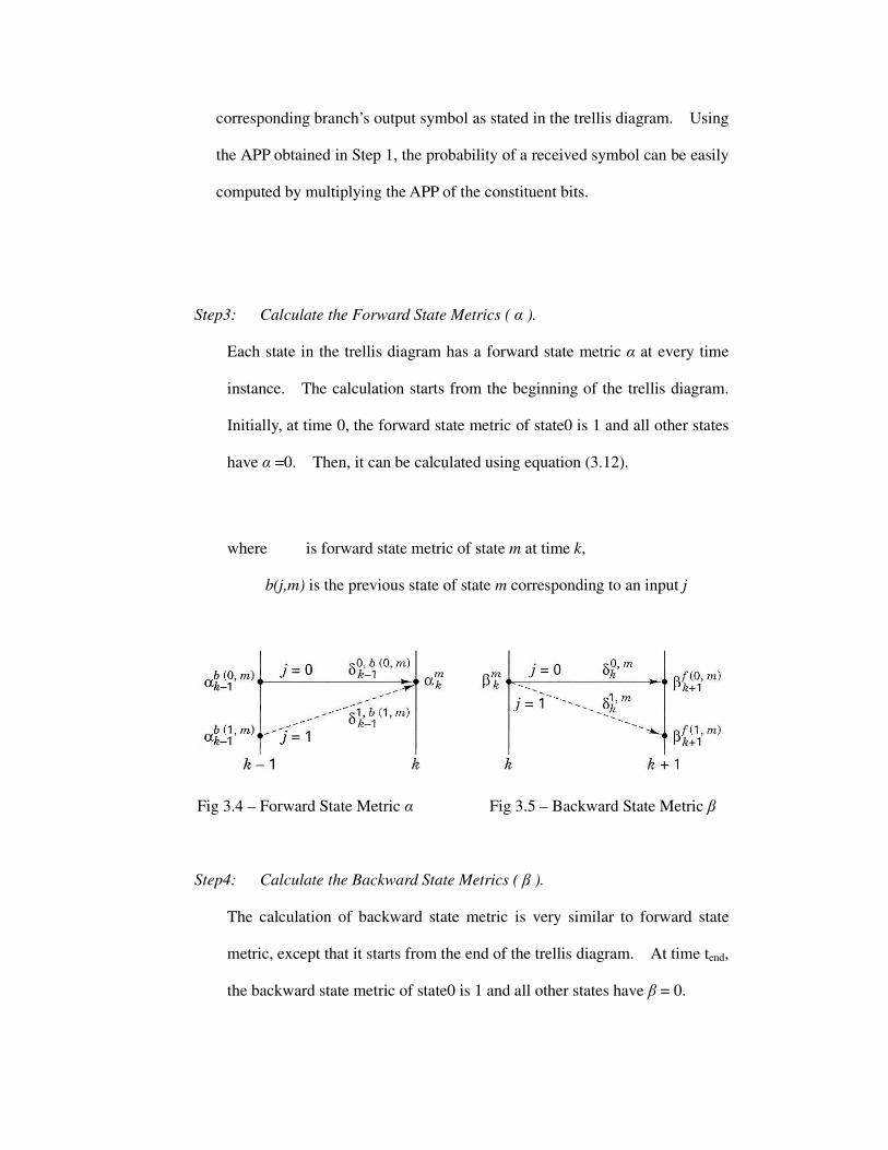
Step3: Calculate the Forward State Metrics
Each state in the trellis diagram has a forward state metric
instance. The calculation starts from the
Initially, at time 0, the forward state metric of s
have α =0. Then, it can be calculated using equation
where is forward state metri
b(j,m) is the previous state of state
Fig 3.4 – Forward State Metric
Step4: Calculate the Backward State Metrics
The calculation of backward state metric is very similar to forward state
metric, except that it starts from the end of the trellis diagram.
the backward state metric of state0 is 1 and all other states have
branch’s output symbol as stated in the trellis diagram. Using
the APP obtained in Step 1, the probability of a received symbol can be easily
plying the APP of the constituent bits.
Calculate the Forward State Metrics ( α ).
Each state in the trellis diagram has a forward state metric α at every time
The calculation starts from the beginning of the trellis diagram
0, the forward state metric of state0 is 1 and all other states
hen, it can be calculated using equation (3.12).
forward state metric of state m at time k,
is the previous state of state m corresponding to an input j
Metric α Fig 3.5 – Backward State Metric
Calculate the Backward State Metrics ( β ).
of backward state metric is very similar to forward state
it starts from the end of the trellis diagram. At time
backward state metric of state0 is 1 and all other states have β = 0.
. Using
can be easily
every time
trellis diagram.
is 1 and all other states
State Metric β
of backward state metric is very similar to forward state
At time tend,

- 9 -
=>? � 1 @A>B,? ! =>C�D�B,?�EB �3.13�
where =>? is backward state metric of state m at time k,
f(j,m) is the next state of state m given an input j
Step5: Calculate the branch probability in the trellis diagram.
The branch probability for each branch in the trellis diagram is calculated by:
Branch Probability � αRS ! δRU,S ! βRC�D�B,?� �3.14�
Step 6: Decode the transmitted sequence.
Each branch in the trellis has an associated input symbol. However, one
input symbol can be associated with more than one branch. Thus, the
summation of the branch probabilities corresponding to a particular input
symbol has to be considered. The one with the highest probability is
chosen to be the decoded result.
E. Superposition Coded Modulation
Transmitter of SCM:
Superposition coded modulation can be classified into two classes: single-code
SCM (SC-SCM) and multi-code SCM (MC-SCM). In both SC-SCM and
MC-SCM, the transmitted signal x is the weighted sum of the coded symbols xk
in all the K layers. W> is the weighting constant for power allocation of the
symbol in the kth
layer.
� � 1 W>�> X>3� �3.15�

- 10 -
The major difference between SC-SCM and MC-SCM is that the former uses a
single common encoder for all the K layers while the latter uses K independent
encoders for each layer. Their transmitter structures are illustrated in Figure 3.6
and Figure 3.7 respectively. MC-SCM with convolutional encoder is used in
this project.
Fig 3.6 – Transmitter structure of SC-SCM
Fig 3.7 – Transmitter structure of MC-SCM
Receiver of SCM:
The receiver structure of MC-SCM is shown in Figure 3.8. The convolutional
decoder uses the same BCJR algorithm as described previously, except that it
also outputs the extrinsic LLRs for iterative decoding.
Fig 3.8 – Receiver structure of MC-SCM
- 11 -
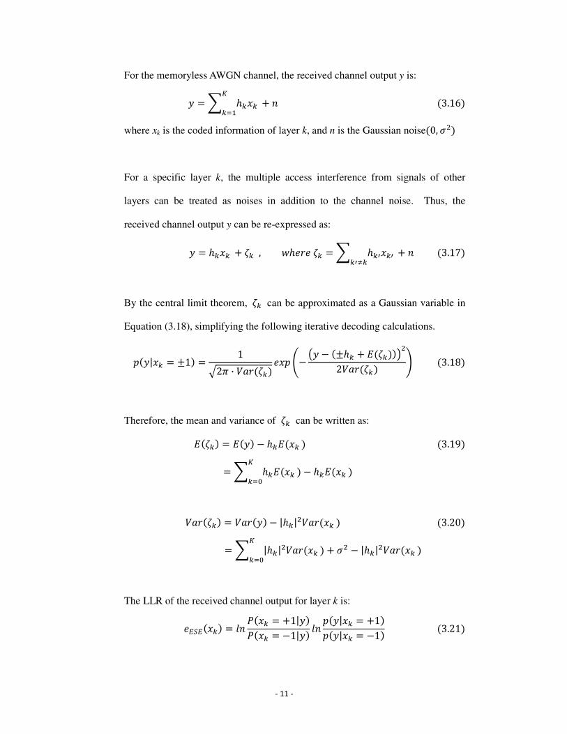
For the memoryless AWGN channel, the received channel output y is:
� � 1 W>�> X>3� ) * �3.16�
where xk is the coded information of layer k, and n is the Gaussian noise�0, ���
For a specific layer k, the multiple access interference from signals of other
layers can be treated as noises in addition to the channel noise. Thus, the
received channel output y can be re-expressed as:
� � W>�> ) Y> , ZW [ Y> � 1 W>\�>\ >\]> ) * �3.17�
By the central limit theorem, Y> can be approximated as a Gaussian variable in
Equation (3.18), simplifying the following iterative decoding calculations.
���|�> � ^1� � 1_2� · a%[�Y>� �� b� c� � �^W> ) d�Y>��e�
2a%[�Y>� f �3.18�
Therefore, the mean and variance of Y> can be written as:
d�Y>� � d��� � W>d��> � �3.19�
� 1 W>d��> �X>3 � W>d��> �
a%[�Y>� � a%[��� � |W>|�a%[��> � �3.20�
� 1 |W>|�a%[��> �X>3 ) �� � |W>|�a%[��> �
The LLR of the received channel output for layer k is:
�g���>� � 6* ,��> � )1|��,��> � �1|�� 6* ���|�> � )1�
���|�> � �1� �3.21�

- 12 -
Substituting Equation (3.18) into Equation (3.21), we have
�g���>� � 2W> �� � d�Y>�a%[�Y>� � �3.22�
The de-interleaved �g��h>� is then fed into the BCJR decoder. After
decoding, the BCJR decoder outputs an extrinsic LLR i�j�h>� for each
received bit, which can be found by subtracting the original channel output
�g��h>� from the decoder output 55�kll�h>� . Then, i�j�h>� is
interleaved and passed back to the ESE for the next iteration decoding by
updating the mean and variance of the layer k signal.
i�j�h>� � 55�kll�h>� � �g��h>� �3.23�
d��> � � &%*W � i�j��>�2 � �3.24�
a%[��> � � 1 � �d��> ��� �3.25�
Hence, the mean and variance of the received channel output y for the next
iteration can be obtained by:
d��� � d�Y>� ) W>d��> � �3.26�
a%[��� � a%[�Y>� ) |W>|�a%[��> � �3.27�
As iterations go on, information of all the K layers can be decoded to a certain
level of reliability.

- 13 -
IV. SIMULATION RESULTS AND ANALYSIS
A. Verification:
The simulation package is developed from a source code which includes i) a
non-systematic and non-recursive convolutional encoder of rate 1/2 using generator
representation, and ii) a universal BCJR decoder of rate 1/2.
In this project, the code table representation derived from its trellis-diagram is
adopted instead to describe the convolutional encoder. Thereby, any structures of
the convolutional encoder of any code rate of k/n can easily be described and
implemented in the simulation package. The universal BCJR decoder is also
amended to decode for any code rate of k/n. Verification of the modified
simulation package is done by BER performance comparison. The reference
results from [3] use Viterbi decoding for unquantized AWGN channel outputs with
32 path memories, which provide very close BER performance to BCJR decoding.
BPSK modulation is used in both the simulated package and the reference results.
Figure 4.1 – Verification for rate 1/2 convolutional code
- 14 -
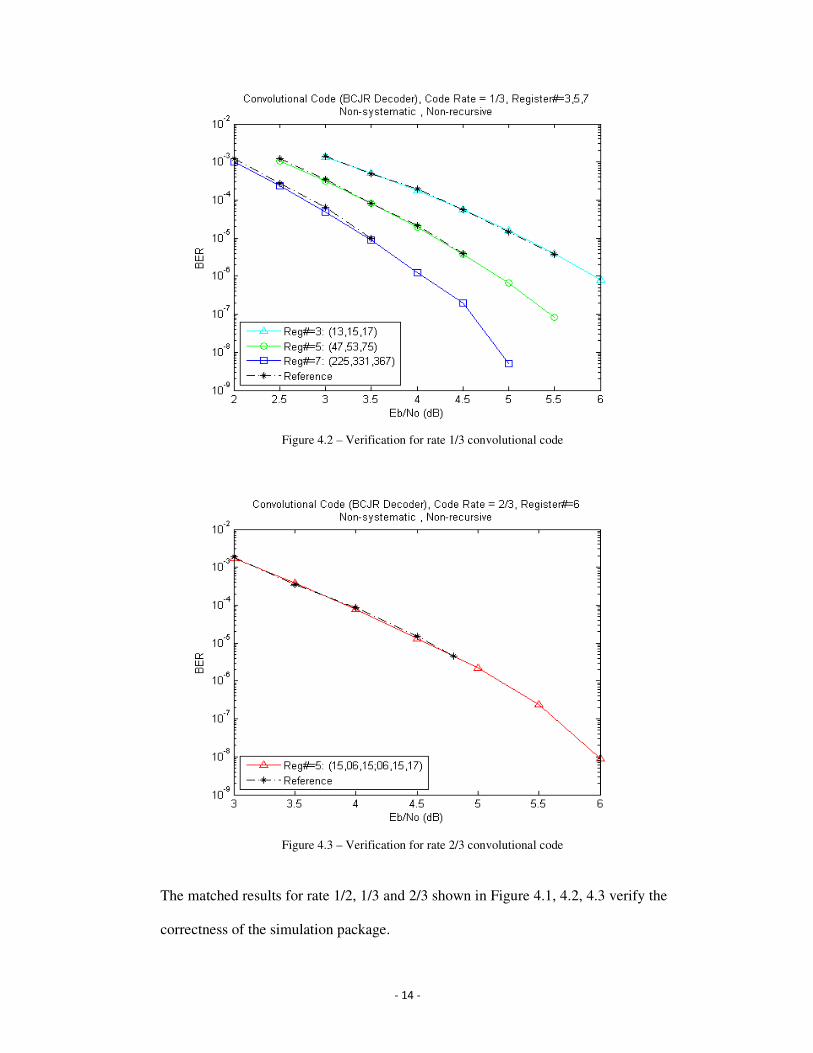
Figure 4.2 – Verification for rate 1/3 convolutional code
Figure 4.3 – Verification for rate 2/3 convolutional code
The matched results for rate 1/2, 1/3 and 2/3 shown in Figure 4.1, 4.2, 4.3 verify the
correctness of the simulation package.

- 15 -
B. Effect of i) Code Rate and ii) Number of Registers:
Figure 4.4 – Effect of Code Rate
The BER performance of convolutional coding with different code rates is
compared in Figure 4.4. Results show that the BER performance can be improved
by using a lower code rate as there is more coded information to provide more
reliable decoding. In addition, the coding gain for the convolutional coding
scheme compared to uncoded BPSK can be observed. The coding gain is
increased by using lower code rate, however, at the cost of lower channel
transmission efficiency.
The BER performance can also be improved by increasing the number of shift
registers in the encoder as observed from Figure 4.1 and 4.2. It is because more
previous input is utilized to encode a symbol which in turn provides more
information for decoding. However, the computational cost also increases.

C. Systematic vs. Non-systematic
Figure 4.5a – Systematic vs. NonFigure 4.5b – Systematic, Recursive Convolutional Encoder used in Fig
The BER performance of different
shift registers is shown in Figure 4.5a. It is observed that non
can outperform systematic encoder in BER since the non
contains more coding information
applications where rough estimation of the received
decoding because part of the transmitted
information. Figure 4.5a also shows that the
lower BER than systematic non
Results from Figure 4.1 to 4.5 show that the
applied to improve the BER
encoder structure can be adopted to meet the system
ystematic and Recursive vs. Non-recursive:
ystematic vs. Non-systematic, Recursive vs. Non-recursive (left)Recursive Convolutional Encoder used in Fig4.5a (right)
different encoder structures at the same rate 1/2 with two
shift registers is shown in Figure 4.5a. It is observed that non-systematic encoder
encoder in BER since the non-systematic encoder output
information. However, systematic encoder is more useful
s where rough estimation of the received information is required before
decoding because part of the transmitted sequence is exactly the original
information. Figure 4.5a also shows that the systematic recursive encoder gives
non-recursive encoder due to its feedback nature.
Results from Figure 4.1 to 4.5 show that the convolutional coding scheme can be
applied to improve the BER performance. Different code rates and different
encoder structure can be adopted to meet the system requirements.
recursive (left) 5a (right)
encoder structures at the same rate 1/2 with two
encoder
encoder output
ful to
is required before
is exactly the original
ecursive encoder gives
coding scheme can be
ifferent code rates and different

- 17 -
D. Performance of convolutional coding in MC-SCM:
A major advantage for SCM is that the overall system rate can easily be adjusted by
accommodating different number of layers for adaptive channel allocation with
reasonable complexity of implementation. In this section, the performance of
convolutional coding in MC-SCM with BPSK modulation is studied.
a) Non-systematic and Non-recursive (5,7) convolutional code of rate=1/2
Figure 4.6 – (5,7) Convolutional Coded MC-SCM with Equal Power Allocation
In Figure 4.6, both the two-user (2 layers) MC-SCM and uncoded BPSK have an
overall system rate of 1. At lower Eb/No, the BER of the two-user SCM is even
poorer than that of the uncoded BPSK system as the multiple access interference is
comparatively too significant. However, at higher Eb/No starting from 4dB, the
two-user SCM has its BER very close to that of the single-user. This means that
SCM can compensate the system rate reduction from coding providing that the
signal power is strong enough to overcome the multiple access interference.

- 18 -
b) Non-systematic and Non-recursive (23,35) convolutional code of rate=1/2
Figure 4.7 – (23,35) Convolutional Coded MC-SCM with Equal Power Allocation
Figure 4.7 shows similar results to Figure 4.6. By using 16-state (23,35)
convolutional coding, the two-user MC-SCM matches the single-user performance
starting from 3dB rather than 4dB. The improvement comes from the (23,35)
convolutional coding itself. However, as shown from the graph, SCM with equal
power allocation does not seem to work at system rate greater than 1. This can be
solved by using spreading and unequal power allocation.
The effect of spreading on (23,35) convolutional coded MC-SCM with equal power
allocation is illustrated in Figure 4.8. The overall system rate for 17-user, 20-user,
22-user and 23-user are 1.0625, 1.25, 1.375 and 1.4375 respectively. By using a
spread length of 8, the bottleneck of the overall system rate is increased from 1 to
about 1.4 although higher signal power is required. Spreading is helpful as the
average of the spreaded bits is utilized for decoding.
- 19 -
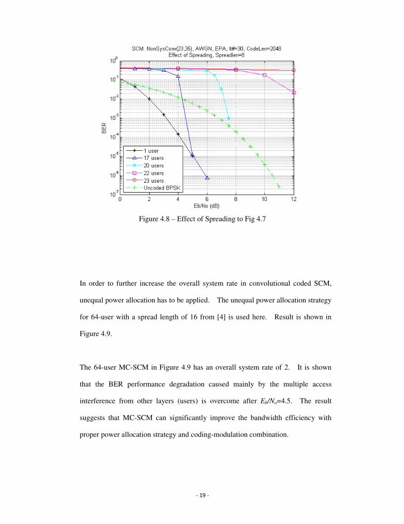
Figure 4.8 – Effect of Spreading to Fig 4.7
In order to further increase the overall system rate in convolutional coded SCM,
unequal power allocation has to be applied. The unequal power allocation strategy
for 64-user with a spread length of 16 from [4] is used here. Result is shown in
Figure 4.9.
The 64-user MC-SCM in Figure 4.9 has an overall system rate of 2. It is shown
that the BER performance degradation caused mainly by the multiple access
interference from other layers (users) is overcome after Eb/No=4.5. The result
suggests that MC-SCM can significantly improve the bandwidth efficiency with
proper power allocation strategy and coding-modulation combination.

- 20 -
Figure 4.9 – Effect of Unqual Power Allocation to Fig 4.7
c) Non-systematic and Non-recursive (25,27,33,35,35,37) 16-state convolutional
code of rate=1/6
Figure 4.10 – Rate-1/6, (25,27,33,35,35,37) Convolutional Coded MC-SCM
with Equal Power Allocation

- 21 -
Figure 4.10 shows the simulation result for a rate-1/6 16-state convolutional coded
MC-SCM with equal power allocation. The overall system rate for single-user,
4-user and 6-user SCM are 1/6, 2/3 and 1 respectively. The 6-user rate-1/6 SCM
matches the single-user BER performance starting from 3.25dB, which is slightly
higher than that of 3dB when comparing to Figure 4.7. This is because the
multiple access interference is more severe in the 6-user rate-1/6 SCM than 2-user
rate-1/2 SCM. However, due to the fact that lower convolutional code rate
provides better BER performance, there is only a slightly increase of 0.25dB in the
threshold. In addition, the lower code rate enhances the flexibility of system rate
adjustment by reducing the increment step size.
From the previous results in Figure 4.6 to 4.10, it is demonstrated that Superposition
Coded Modulation can build up a high rate system by using low rate coding with
simple modulation scheme. The low rate coding enhances the BER performance
as well as the system rate adjustment flexibility. And the simple modulation
scheme greatly reduces the system hardware complexity by avoiding the use of
sophisticated constellation. Therefore, it can be said that SCM can provide an
easy solution to adaptive channel allocation by accommodating different amount of
layers with relatively simple hardware implementation.

- 22 -
V. CONCLUSION
In this project, a universal simulation package for convolutional coding using the
BCJR decoding algorithm has been successfully developed. The simulation package
was first verified with reference results and was then used to study the BER
performance of convolutional coding. After that, the convolutional coding
simulation package is applied in a multi-coded Superposition Coded Modulation
(MC-SCM). From the simulation results, the effects of MC-SCM have been studied.
It is observed that SCM is very suitable for adaptive channel allocation. The use of
low rate code and simple constellation to build up a high rate system greatly reduces
the implementation complexity.

- 23 -
REFERENCE
[1] L.H. Charles Lee, “Convolutional Coding : Fundamentals and Applications”, Artech House, pp.
225-228, 1997
[2] Martin Bossert, “Channel Coding for Telecommunications”, Wiley, p. 202, p.204, p.210, 1999
[3] Shu Lin, Daniel J. Costello, “Error control coding: fundamentals and applications”, (2nd Edition),
Prentice Hall, pp. 555-557, 2004
[4] Li Ping, Lihai Liu, Keying Wu, and W. K. Leung, “Interleave Division Multiple-Access”, IEEE
Trans. Wireless Commun., vol. 5, no. 4, pp. 938-947, Apr. 2006.