Artificial evolution of controllers based on

non-linear oscillators for bipedal locomotion

Julien Nicolas

December 16, 2005

Master Thesis, winter 2005-2006Computer and Communication Sciences

Supervisor: Ludovic Righetti, BIRG EPFLProf. resp: Auke Jan Ijspeert, BIRG EPFL

Contents

1 Acknowledgments 5

2 Objectives 6

3 Introduction 73.1 Biological bipedal locomotion . . . . . . . . . . . . . . . . . . 73.2 Bipedal locomotion in robotics . . . . . . . . . . . . . . . . . 8

3.2.1 Trajectory based methods . . . . . . . . . . . . . . . . 83.2.2 Heuristic control methods . . . . . . . . . . . . . . . . 93.2.3 CPG and reflex methods . . . . . . . . . . . . . . . . . 11

4 The robot 144.1 Real biped robots . . . . . . . . . . . . . . . . . . . . . . . . . 144.2 The simulator . . . . . . . . . . . . . . . . . . . . . . . . . . . 15

5 The CPG model 165.1 Open-loop . . . . . . . . . . . . . . . . . . . . . . . . . . . . . 16

5.1.1 Hopf oscillator . . . . . . . . . . . . . . . . . . . . . . 165.1.2 Rayleigh’s oscillator . . . . . . . . . . . . . . . . . . . 235.1.3 Matsuoka’s oscillator . . . . . . . . . . . . . . . . . . . 25

5.2 Closed-loop . . . . . . . . . . . . . . . . . . . . . . . . . . . . 285.2.1 Speed adaptation and pendulum effect compensation . 29

6 The genetic algorithm 306.1 The genome . . . . . . . . . . . . . . . . . . . . . . . . . . . . 30

6.1.1 Hopf model . . . . . . . . . . . . . . . . . . . . . . . . 316.1.2 Rayleigh model . . . . . . . . . . . . . . . . . . . . . . 316.1.3 Matsuoka model . . . . . . . . . . . . . . . . . . . . . 32

6.2 The algorithm . . . . . . . . . . . . . . . . . . . . . . . . . . . 326.3 The fitness function . . . . . . . . . . . . . . . . . . . . . . . 326.4 The GA parameters . . . . . . . . . . . . . . . . . . . . . . . 33

2

7 Analysis of the results 347.1 Open-loop . . . . . . . . . . . . . . . . . . . . . . . . . . . . . 34

7.1.1 Hopf’s oscillator . . . . . . . . . . . . . . . . . . . . . 347.1.2 Rayleigh’s oscillator . . . . . . . . . . . . . . . . . . . 367.1.3 Matsuoka’s oscillator . . . . . . . . . . . . . . . . . . . 37

7.2 Closed-loop . . . . . . . . . . . . . . . . . . . . . . . . . . . . 417.2.1 Speed adaptation . . . . . . . . . . . . . . . . . . . . . 417.2.2 Resistance against perturbations . . . . . . . . . . . . 49

8 Conclusion 518.1 The project . . . . . . . . . . . . . . . . . . . . . . . . . . . . 518.2 Further work . . . . . . . . . . . . . . . . . . . . . . . . . . . 52

3

4

Chapter 1

Acknowledgments

I would like to deeply thank my supervisor, Ludovic Righetti, for his pre-cious advices as well as for his theoretical and technical support.I would also like to thank Auke Ijspeert and the BIRG for giving me theopportunity to work in such an interesting field as bio-inspired robotics.

5

Chapter 2

Objectives

Millions of years of evolution made humans able to walk and run with anincredible precision. Although bipedal locomotion could seem to be a simplemechanical problem, researches done on artificial locomotion proved that itis far from obvious to generate a walking gait that is as fast and stable ashumans do.In this work, we will directly inspire us from biological considerations byusing CPG based controllers and artificial evolution. First, several modelsof CPGs, implemented on a simulated robot, will be explored using geneticalgorithms to find which system is best suited to locomotion. After that,we will try to improve our model by adding feedback pathways in the CPGsin order to be able to modify the speed of locomotion. In the same time,feedback pathways will be used to let our robot deal with external pertur-bations.

6

Chapter 3

Introduction

3.1 Biological bipedal locomotion

Amongst all skills of living species, locomotion is certainly one of the cru-cial ability that emerged from millions of years of evolution. Almost eachspecies, going from unicellulars to humans, developed a form of locomotionperfectly suited to its morphology and environment to ensure its survival.In spite of the huge diversity of the animal reign, it has been shown thatanimals, and in particular vertebrates, share some common properties al-though they use completely different forms of locomotion [9].To achieve locomotion the neural system generates rhythmic signals that aresent to the musculo-skeletal system in order to produce torques on the differ-ent joints of the animal [2]. Locomotion can be described by the interactionof three elements:

1. spinal central pattern generators (CPG).

2. sensory feedback.

3. descending supra-spinal control.

Bipedal locomotion seems to be more complicated than the process shownabove since the balance is much more important with only two legs, makingcontrol crucial. It is not proved that humans use a simple CPG basedlocomotion like a lamprey or a fish would do, but we still have some evidencesthat the locomotion pattern are generated at the spinal level and are sentthrough the reticulospinal pathways. We can consider that humans use asystem that is comparable to a CPG for their locomotion.Studying bipedal locomotion in animals and in particular humans, gives us agood idea on how their gait could be modeled. Although bipedal locomotionhas been studied by scientists of different domains, this problem has not beencompletely solved yet.

7

3.2 Bipedal locomotion in robotics

Researches made on bipedal locomotion in robotics have shown that we mustmainly consider three different approaches to control walking:

Statically stable walking This corresponds to the case when theprojection on the ground of the robot’s center of gravity always lies withinthe footprint or the area between the two footprints of the robot. With thishypothesis the locomotion is quite easier to perform but is very slow.

Dynamic walking In this case, the robot’s center of gravity can beelsewhere and corrections must be done at any time to maintain the roboton his feet. To achieve stability in those conditions it is mandatory to knoweverything from the robot’s dynamics and in particular the speed and inertiaof each of its parts. This method is without a doubt the more efficient interms of velocity but is very tricky to implement. It also corresponds to thehuman locomotion.The next section introduces different approaches based on dynamic walking.

Passive walking A third type of biped locomotion that has been stud-ied by many researchers is called passive walking [6]. In this case no actua-tors are used and the robot uses its own weight and dynamics to walk downa slope without external input or control. The system has a stable limitcycle and the robots are even able to deal with small perturbations. Wecan also mention the concept of passive dynamic walkers. In this case smallpower sources on their ankles and/or hips are included to simulate gravity,which allows the robots to walk on a level ground without control servos.This approach is very important since it allows to learn many features ofrobot’s dynamics that are also useful for other kind of locomotion [5, 4].

3.2.1 Trajectory based methods

The basic idea of this method is to find walking trajectories and uses acriterion based on dynamic equations to test and prove that the locomotionis stable. These trajectories could be designed by trial-and-error or frompredefined human recordings (motion capture). This approach does notprovide any methodology to implement locomotion in a robot. It only allowsto prove and measure the stability of the gait which is still an useful tool toanalyze artificial motion.In 1990, Vukobratovic [7] proposed a method called Zero Moment Point(ZMP) which seems to be the most promising trajectory based method.The Zero Moment Point is the point on the ground where the moment ofinertial forces and gravitational forces has no component along the horizontalplane. To achieve the stability of the locomotion, the ZMP must always be

8

located within the robot’s footprint. We can also notice that Vukobratovicdistinguishes to different phases: single-support when only one foot touchesthe ground and double-support when both feet are on the ground. Duringthis last phase, the locomotion is stable if the ZMP is located betweenthe two footprints. This method also allows to deal with perturbations byintroducing online stabilization.This method has been successfully implemented on several robots such asSony’s QRIO and Honda robot.

Advantages

• Can be used to prove stability.

• Resistant against small perturbations.

• Well-suited for implementations on real robots.

• Can be adapted to dynamic walking.

Drawbacks

• A perfect knowledge of the robot’s dynamics is mandatory.

• Not suited for unknown environment.

• Switching from online control to wanted trajectory is hard to achieve.

• Not suited to design locomotion controllers.

3.2.2 Heuristic control methods

As the ZMP method does not provide any methodology to design controllers,heuristics were developed to deal with that problem. In addition, heuristicsdecrease considerably the complexity of the dynamic equations involved intrajectory based methods and make implementation much easier.One of the most efficient and interesting method using heuristics calledVirtual Model Control (VMC) has been developed by J. Pratt [8] at theMIT’s Leglab. This approach is based on virtual mechanical componentslike springs, dampers, dashpots,... These elements generate real torques orforces on the actuators. These torques create the same effect as that thevirtual components would have produced if they were real. This methodallows to achieve different kinds of movements just by choosing the appro-priate virtual elements. The torque needed to produce the virtual force istypically computed using the Jacobian relating the reference frame of thevirtual component to the robot.In practice, movements are relatively easy to implement on controllers. Foreach different motion or behavior, an appropriate set of virtual components

9

has to be defined. For example, to maintain the robot in an upright andstable position, a kind of granny walker has to be introduced as virtual com-ponent to guarantee stability. To make the robot walk, a typical componentis a virtual dogtrack bunny associated with a damper mechanism (cf fig 3.1).This model implies to consider different states to deal with the different ac-tuation phases this means that, in a given phase, only certain motors areactivated. This problem can be solved using a finite state machine.The MIT’s Leglab successfully implemented the method described above ontheir Flamingo and Turkey robots1

Figure 3.1: Example of virtual components

Advantages

• Detailed methodology to design controllers.

• Very intuitive approach.

• Complete knowledge of the environment is not required.

• Can deal with small perturbations.1More details are given in [8]

10

• Efficient online control.

Drawbacks

• A perfect knowledge of the robot’s dynamics is mandatory.

• The designer must ensure that the torques generated on the joints aresupported by the robot to avoid damages.

• The mechanism based on finite state machines causes brutal transi-tions between the different phases.

3.2.3 CPG and reflex methods

The approach described in this section is based on Central Pattern Generator(CPG) and is directly inspired from biological considerations as mentionedin section 3.1. The main advantage of this method, compared to those de-scribed above, is that here, we do not need a perfect knowledge of the robot’sdynamics. It is a more general and adaptive method to design controllersfor bided robots. Reflexes are produced by the robot’s feedback sensors andare used to manage perturbations and balance control.The work done by Taga [11] proves that CPGs and reflexes can be used forlocomotion on biped robots.CPGs can be represented by different mathematical models such as oscil-lators, artificial neurons, vector fields,... Each CPG usually represent onedegree of freedom (DOF) of a joint. Oscillator based CPGs are using theconcept of limit cycles which are very convenient in the case of locomotionsince they can return to their stable state after a small perturbation and arealmost not influenced by a change in the initial conditions.

CPG and reflex loop Different models could be used to represent the in-teraction between the CPG and the reflex system. The choice of the systemdepends on the complexity of the feedback mechanism we want to represent.Note that a system with complicated feedback will be much more difficultto design as more parameters are involved in the system. Some models offeedback pathways are described below.

Open-loop Here, we present a simple model based on CPGs knownas open-loop model (cf. fig 3.2). The CPG interacts directly with theactuators but receives no feedback from the sensors and the actuators (open-loop). Such a model has the advantage that it allows a relatively simpleimplementation since no sensors are used. However it is not very well suitedto deal with perturbations in the environment.

11

Figure 3.2: A simple open-loop model with no feedback. This model will beused in the first part of this project

Closed-loop In this case, we use sensor feedback to close the loop, thismeans that the CPG receives information from different kinds of sensors.The simplest method is to consider feedback pathways going only from theactuators to the CPGs (cf. fig 3.3). This approach allows us to maintain asystem that is still relatively simple to represent and has the ability to berobust against small external perturbations.A more complete and promising closed-loop model consists of three levels offeedback (cf. fig 3.4):

1. The fast reflex interferes directly on the joint’s actuators and do notmodify the CPG. It should correct the robot’s position very quickly.

2. The CPG reflex influences the middle level of the system and corre-sponds to the feedback used on the simplified version of the closed-loopmodel described above. This kind of feedback has been introduced todeal with external perturbations such as wind, ground deformation,...

3. The global reflex interacts with the system on its higher level and willbe used to modify the global behavior of the robot when encounteringa new situation such as a slope.

In addition to the mechanism described above, two control system are added:

1. The visual system interacts with the CPG and directly with the actu-ators.

2. The vestibular system is also connected to the CPGs and the actua-tors. It is used to control the global balance of the robot.

This method seems to be very promising since it has already been success-fully implemented on an artificial lamprey [14] and more recently on anartificial salamander [12] that even has the ability to switch between swim-ming and walking [13].

12

Figure 3.3: A minimal closed-loop model. Only the actuators interact withthe CPGs

Figure 3.4: A closed loop model with three different reflexes type influencingdifferent parts of the system. On the top left, the visual system interactswith the CPG and directly on the actuators. The vestibular system controlsthe balance of the robot and influences the CPG and the actuators.

Advantages

• A perfect knowledge of the robot’s dynamics is not required.

• Robust against small perturbations.

• Almost not influenced by a change in the initial conditions.

• Oscillations produce smooth locomotion.

• Complex control input not required since the oscillation is generatedby itself.

Drawbacks

• No clear methodology to design controllers.

• Parameters are hard to find by hand. So it is recommended to uselearning algorithms.

13

Chapter 4

The robot

4.1 Real biped robots

In this last decade a lot of improvements have been done in the developmentof autonomous biped robots. Big companies like Honda, Fujitsu or Sonybegan developing expensive robots for research. Since a few year, robotslike Qrio or Sony’s Aibo are available at a reasonable price and are subjectto several studies.In this project, we will focus on Fujitsu’s robot called HOAP 2 (Humanoidfor Open Architecture Platform) [23]. HOAP 2 is 50 cm tall and is only 7kg which makes it really easy to handle. Its 24 degree of freedom allows itto perform a lot of movements including hands and head control (fig 4.1).This robot also has servo angle sensors, gyroscope and pressure sensors intheir feet, useful for locomotion with feedback.

14

Figure 4.1: Left: The Hoap2 robot. Right: The different DOFs available onHoap 2

4.2 The simulator

One of the drawbacks of these robots is that they are very fragile and expen-sive. As artificial evolution will be used to tune the controller parameters,we expect the robot to fall hundred times before finding a good trajectory.Experimenting controllers on the real robot would then certainly break it.Another advantage of simulated robots in the context of this project is thatwe can launch many simulations with different parameters.The reasons given above clearly encouraged us to perform our research on asimulated robot. For this purpose, we used Webots [20], which is a completetoolkit to model, program and test robot’s behaviors in their environment.Webots is developed by Cyberbotics and has become a reference softwareused by many universities and researchers. This software includes many use-ful devices such as cameras, light sensors, touch sensors, emitters/receivers,gps,... One of the most powerful feature of Webots is its fully customizableVRML based environment. For example, this will allow us to add externalperturbations such as wind, slopes, steps,... This simulator also uses a pow-erful dynamic engine based on ODE (Open Dynamic Engine), which is anopen-source library for simulating rigid body dynamics.Webots also provides a collection of existing robots including Hoap 2 thatwas designed by Pascal Cominoli during his Master’s thesis at the BIRG(EPFL) [21]. This virtual robot corresponds exactly to the real one in termsof weight, size and servo specifications.

15

Chapter 5

The CPG model

As described in 3.2.3 the model studied in this work uses Central PatternGenerators to control the robot’s servos. To represent these CPGs and togenerate signals, we use one or several non linear oscillators that are coupledtogether. A very interesting property of non linear oscillators is the conceptof limit cycle [15][16]. A limit cycle can be described as an isolated closedtrajectory of the system, which can be stable or unstable. The first case isvery important since all trajectories close to the limit cycle are attracted byit. This principle will be useful to generate robust signals that can return totheir stable position after a small perturbation. This section describes thedifferent oscillators and coupling models used in this work.For each experiment described in this chapter, we will use a simplified modelof the robot this means that not all the servos will be used since some ofthem are not relevant for locomotion. We will then focus on 11 servos (1 forthe body, 2 for each hip, 1 for each knee and 2 for each ankle). Both legsare connected to the body’s servo and a phase difference of π is imposedbetween them since there is an obvious symmetry between the joints’ anglesof each leg. The servos responsible for the twist of the hip and the ankle arenot used because they do not play an important role in walking.As the servos’ position is not always oscillating around 0, we add a bias tothe output of each oscillators. Note that this bias will also be evolved andis used in every model described below.

5.1 Open-loop

5.1.1 Hopf oscillator

The first model used in this work is based on the Hopf’s oscillator, a rela-tively simple system for preliminary experiments. Its main advantage is thepossibility to easily control the amplitude and the frequency of the signalindependently. The following equations describe this oscillator.

16

x = (µ− r2)x− ωy (5.1)y = (µ− r2)y − ωx (5.2)

Where r =√

x2 + y2, µ > 0 determines the amplitude of the signal and ωcontrols the frequency of the oscillator. This oscillator has a stable limitcycle with radius

√µ and angular velocity ω rad/s.

Figure 5.1: Phase plot of the Hopf’s oscillator with different initial condi-tions. Here we set µ = 1.0 and ω = 1.0.

The coupling

1-way coupling With this first model, we will start with a one-way cou-pling, It acts only from one oscillator to the other in one direction (not inreverse) as shown on figure 5.2. This coupling is described by the followingequations

xi = (µi − r2i )xi − ωyi + εixi−1 (5.3)

yi = (µi − r2i )yi − ωxi (5.4)

Where εi is the coupling strength (ε1 = 0 since the first servo is not coupledwith any other joint) and ω has the same value for each oscillator. Withthis coupling model, the amplitude of the coupled oscillator’s signal cannotbe controlled as in the case of a single oscillator. This means that theamplitude depends on the µi parameter but is also influenced by the coupling

17

strength εi. This phenomenon is explained by the fact that the two involvedoscillators are in resonance since their respective frequencies are the same.To deal with this problem, we will set a sufficiently large interval of possiblevalues for the amplitude parameters, which will allow us to roughly setthese values. The genetic algorithm will tune these values more precisely.An interesting property of this coupling model is that we can introduce asimple phase difference by changing the sign of εi. If εi < 0, then the phasedifference is equal to π and if εi > 0 the phase difference is null (cf. fig 5.4).This allowed us to impose phase differences between the different servos asshown on figure 5.2. However, this simple model does not allow to produceother phase differences than those mentioned above and will probably notproduce a very realistic gait. Completely arbitrary phase differences couldhave been introduced by using the two variables xi and yi in the coupling,but this would consequently enlarge the search space of the GA (five extraparameters). As the GA took approximately 12 hours to find a good solutionfor the model described above, we tried to simplify each model used as muchas possible.

Figure 5.2: The different DOF used in this work. The arrows represent theunidirectional coupling of this first model. The values on the arrows corre-spond to the phase differences we imposed between the different oscillators.

18

Figure 5.3: These figures show the first variables (x1 and x2) of two coupledoscillators. We can see here that for εi < 0, the phase difference after afew steps is π (top plot). For εi > 0 we have a phase difference equal to 0(bottom plot). We can also see that the amplitude of x2 is slightly changeddue to the phenomenon of resonance. The parameters used here are thefollowings: µ1 = µ2 = 1.0, ω = 1.0 and ε2 = ±0.3

2-way coupling The second coupling model we are using is the sameas the previous one but with influence in both directions. Two adjacentoscillators are coupled in both directions. Note that the oscillators are alsochained along the leg (cf. fig 5.5). With this coupling we are now able tointroduce more complex phase differences like π/2 and −π/2 as describedin table 5.1. Notice that, to reduce the search space, we set the phasedifferences between the different servos by hand (cf. fig 5.5). These phasedifferences were found empirically after a few tests and seemed to be themost realistic ones for this model. The following equations describe thatmodel.

xi = (µi − r2i )xi − ωyi + εi,i−1xi−1 + εi,i+1xi+1 (5.5)

yi = (µi − r2i )yi − ωxi (5.6)

In this case, there are two parameters for the coupling strength (εi,i−1 andεi,i+1), one for each adjacent oscillator.

19

value of the coupling coefficients ε1,2 and ε2,1 phase differenceε1,2 = ε2,1 > 0 0

ε1,2 > 0 and ε2,1 = −ε1,2π2

ε2,1 > 0 and ε1,2 = −ε2,1, −π2

ε1,2, ε2,1 < 0 and ε1,2 > ε2,1 πε1,2, ε2,1 < 0 and ε1,2 < ε2,1 −π

Table 5.1: Phase differences between two Hopf oscillators with 2-way cou-pling for different value of the coupling coefficients. The relation betweenthese parameters will be used to produce a phase difference between thedifferent servos of the robot.

Figure 5.4: First variables (x1 and x2) of two oscillators coupled in bothdirections. This example shows a phase difference of π/2 between bothsignals. The parameters used here are the followings: µ1 = µ2 = 1.0, ω =1.0, ε1,2 = 0.5 and ε2,1 = −0.5

20

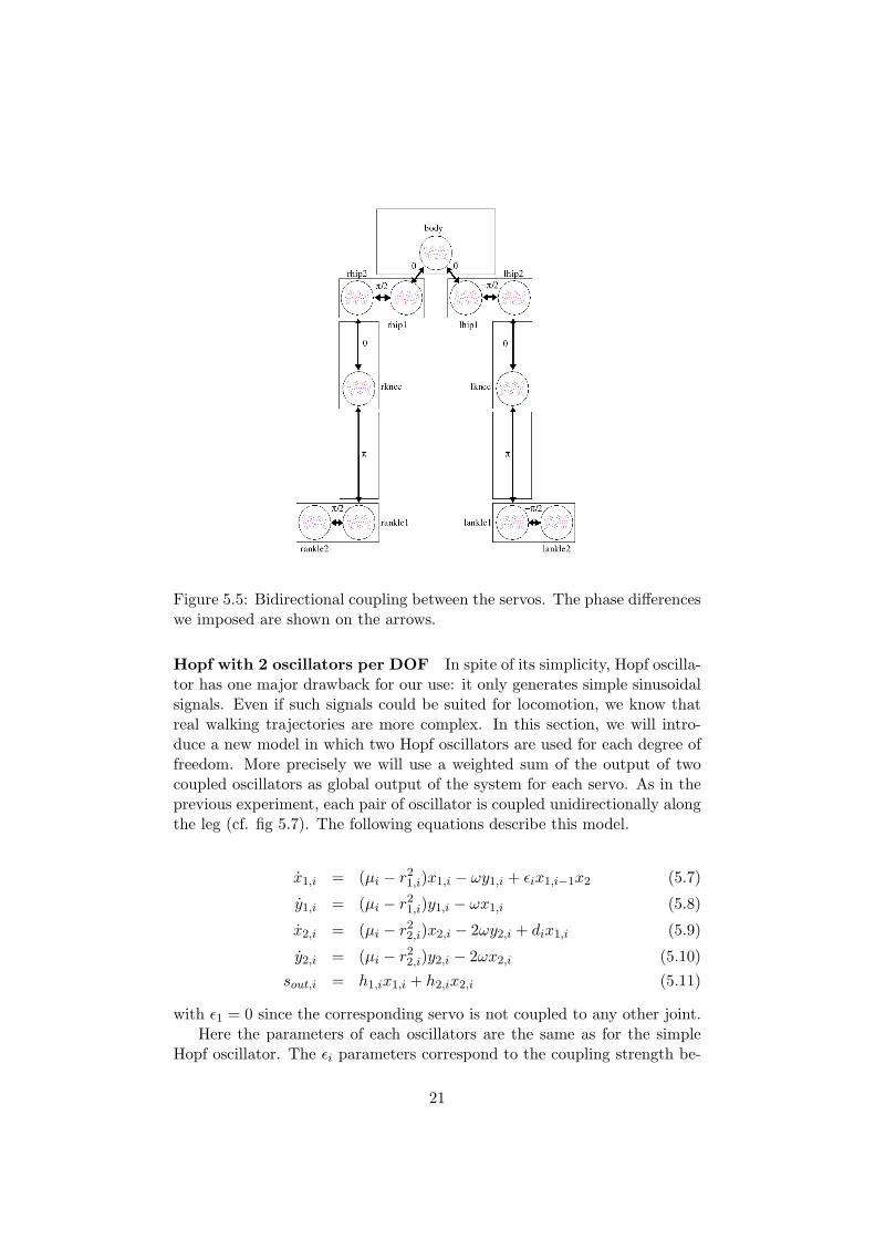
Figure 5.5: Bidirectional coupling between the servos. The phase differenceswe imposed are shown on the arrows.

Hopf with 2 oscillators per DOF In spite of its simplicity, Hopf oscilla-tor has one major drawback for our use: it only generates simple sinusoidalsignals. Even if such signals could be suited for locomotion, we know thatreal walking trajectories are more complex. In this section, we will intro-duce a new model in which two Hopf oscillators are used for each degree offreedom. More precisely we will use a weighted sum of the output of twocoupled oscillators as global output of the system for each servo. As in theprevious experiment, each pair of oscillator is coupled unidirectionally alongthe leg (cf. fig 5.7). The following equations describe this model.

x1,i = (µi − r21,i)x1,i − ωy1,i + εix1,i−1x2 (5.7)

y1,i = (µi − r21,i)y1,i − ωx1,i (5.8)

x2,i = (µi − r22,i)x2,i − 2ωy2,i + dix1,i (5.9)

y2,i = (µi − r22,i)y2,i − 2ωx2,i (5.10)

sout,i = h1,ix1,i + h2,ix2,i (5.11)

with ε1 = 0 since the corresponding servo is not coupled to any other joint.Here the parameters of each oscillators are the same as for the simple

Hopf oscillator. The εi parameters correspond to the coupling strength be-

21

tween the two adjacent systems and the coefficient di allows us to introducea phase difference between the two oscillators of each DOF.The output sent to the servos corresponds to a weighted sum of the first vari-ables of each oscillator. The parameters h1,i and h2,i represent the weightsof this sum. We can also notice that the natural frequency of the secondoscillator (x2,i, y2,i) is the double (and by consequence the first harmonic) ofthe one that rules the first oscillator (x1,i, y1,i). This model is then designedto produce a signal that corresponds to the first two terms of a Fourier seriesand should be closer to the real biped locomotion.

Figure 5.6: Example of evolution of the output sout,i generated by the pairof oscillators described above. We see that the shape of the signal is morecomplex and can be modified by changing the weights of the output sum.Here the parameters are µi = 1.0, ω = 2.0, di = 0.3, h1,1 = 0.4 and h2,1 =0.2.

For this experiment, we kept some parameters found with the simple 1-way Hopf model, in particular we reused the values found for the amplitudesµi, the frequency ω and the bias. So the only parameters that are evolvedhere are the different coupling strengths and weights (εi, h1,i, h2,i and di).The phase difference between two consecutive pairs of oscillators can bemodified by changing the εi parameter as it was done with the simple 1-wayHopf model (cf. fig 5.2).

22

Figure 5.7: Model used with 2 oscillators for each DOF. The same couplingapplies to the right leg. The weight of the different couplings involved isshown on the arrows.

5.1.2 Rayleigh’s oscillator

The oscillator

To explore different signal shapes, we chose to use a relaxation oscillatoras next model. More precisely the model used in this second experimentis based on the Rayleigh’s oscillator. The following equations describe thismodel.

x = y (5.12)y = δ(1− qy2)y − ω2 (5.13)

In order to reduce the search space of the genetic algorithm, we set δ = 1.The q coefficient allowed us to control the amplitude of the signal and theparameter ω was used to modify the frequency. Note that a variation ofω slightly changes the amplitude of the signal, but the genetic algorithmshould deal with that.

23

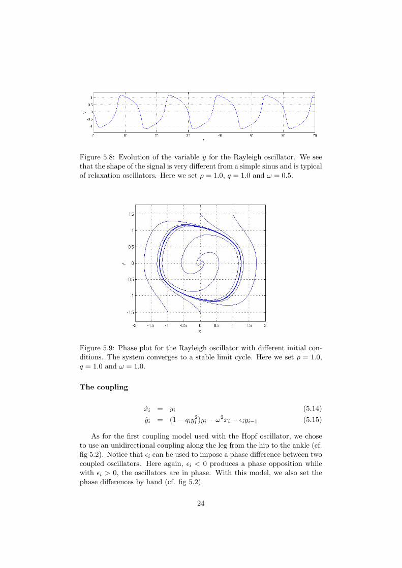
Figure 5.8: Evolution of the variable y for the Rayleigh oscillator. We seethat the shape of the signal is very different from a simple sinus and is typicalof relaxation oscillators. Here we set ρ = 1.0, q = 1.0 and ω = 0.5.

Figure 5.9: Phase plot for the Rayleigh oscillator with different initial con-ditions. The system converges to a stable limit cycle. Here we set ρ = 1.0,q = 1.0 and ω = 1.0.

The coupling

xi = yi (5.14)yi = (1− qiy

2i )yi − ω2xi − εiyi−1 (5.15)

As for the first coupling model used with the Hopf oscillator, we choseto use an unidirectional coupling along the leg from the hip to the ankle (cf.fig 5.2). Notice that εi can be used to impose a phase difference between twocoupled oscillators. Here again, εi < 0 produces a phase opposition whilewith εi > 0, the oscillators are in phase. With this model, we also set thephase differences by hand (cf. fig 5.2).

24

5.1.3 Matsuoka’s oscillator

The oscillator

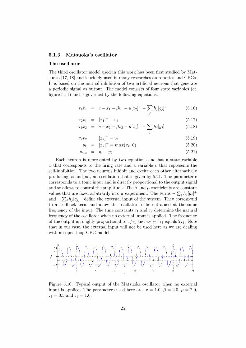
The third oscillator model used in this work has been first studied by Mat-suoka [17, 18] and is widely used in many researches on robotics and CPGs.It is based on the mutual inhibition of two artificial neurons that generatea periodic signal as output. The model consists of four state variables (cf.figure 5.11) and is governed by the following equations.

τ1x1 = c− x1 − βv1 − µ[x2]+ −∑j

hj [gj ]+ (5.16)

τ2v1 = [x1]+ − v1 (5.17)τ1x2 = c− x2 − βv2 − µ[x1]+ −

∑j

hj [gj ]− (5.18)

τ2v2 = [x2]+ − v2 (5.19)yk = [xk]+ = max(xk, 0) (5.20)

yout = y1 − y2 (5.21)

Each neuron is represented by two equations and has a state variablex that corresponds to the firing rate and a variable v that represents theself-inhibition. The two neurons inhibit and excite each other alternativelyproducing, as output, an oscillation that is given by 5.21. The parameter ccorresponds to a tonic input and is directly proportional to the output signaland so allows to control the amplitude. The β and µ coefficients are constantvalues that are fixed arbitrarily in our experiment. The terms −

∑j hj [gj ]+

and −∑

j hj [gj ]− define the external input of the system. They correspondto a feedback term and allow the oscillator to be entrained at the samefrequency of the input. The time constants τ1 and τ2 determine the naturalfrequency of the oscillator when no external input is applied. The frequencyof the output is roughly proportional to 1/τ1 and we set τ1 equals 2τ2. Notethat in our case, the external input will not be used here as we are dealingwith an open-loop CPG model.

Figure 5.10: Typical output of the Matsuoka oscillator when no externalinput is applied. The parameters used here are: c = 1.0, β = 2.0, µ = 2.0,τ1 = 0.5 and τ2 = 1.0.

25

Figure 5.11: The two coupled neurons of the Matsuoka oscillator. The blackcircles correspond to inhibitory connections and white circles to excitatoryconnections. The self-inhibition is governed by the βvi connections whilemutual inhibition is done through the µ[xi]+ connections.

The coupling

The coupling model used for that oscillator is once again an unidirectionalcoupling (cf. fig 5.13). This model has been studied by M. Williamson [19]and seems to be well-suited to our needs. The coupling is done by addingcoupling terms to the equations of x′1 and x′2 as described in equations 5.23to 5.27.With this model it is also possible to introduce a phase difference betweentwo coupled oscillators. The γi parameter can be used to achieve phase dif-ferences of 0, π/2 and π as described in table 5.2.We also set the phase differences between the different servos by hand. Thesevalues are shown in figure 5.12.

26

value of γi phase difference[0.0, 0.3] π[0.3, 0.5] −π/2[0.5, 0.7] π/2[0.7, 1.0] 0

Table 5.2: The phase differences produced by changing the γi coefficient.Notice that for values of γ1 in [0.3, 0.7] the phase difference is not preciselyequal to ±π/2 and varies for some intermediate values of γ1 in this interval.However the GA should find the best values.

Figure 5.12: Couplings between the servos for the model based on Matsuokaoscillators. The phase differences we imposed between the different servosis shown on the arrows.

Notice that, with this model, the signals for the ankle1 servo are notevolved but are computed to be roughly parallel to the ground (cf. figure5.12). The servo position then depends on the hip2 and knee joints’ angleand the ankle2 servo is thus coupled directly to the knee’s oscillator. Wealso fixed some parameter values (the central position of hip1 and ankle2servos were set to 0).

27

τ1x1,i = ci − x1,i − βv1,i − µ[x2,i]+ −− αi,i+1γi[x1,i+1]+ − αi,i+1(1− γi)[x2,i+1]+ (5.22)

τ2v1,i = [x1]+ − v1,i (5.23)τ1x2,i = ci − x2,i − βv2,i − µ[x1,i]+ −

− αi,i+1γi[x2,i+1]+ − αi,i+1(1− γi)[x1,i+1]+ (5.24)τ2v2,i = [x2,i]+ − v2,i (5.25)

yk,i = [xk,i]+ = max(xk,i, 0) (5.26)yout,i = y1,i − y2,i (5.27)

Where αi,i+1 corresponds to the global coupling strength between oscil-lator i and i+1 and γi controls the relative coupling of each neuron.

Figure 5.13: Coupling between two Matsuoka oscillators. They are onlycoupled in one direction (from 1 to 2). Each neuron of 1 (1,i and 2,1) isconnected to both neurons of 2 (1,i+1 and 2,i+1). The relative strength ofcoupling 1,i → 1,i+1 against coupling 1,i → 2,i+1 can be modified throughparameter γi.

5.2 Closed-loop

We will now introduce a more complex CPG model based on the closed-loopconcept. As described above, this concept add the notion of feedback to theopen-loop model. Feedback can be integrated at different levels of the robotdepending of the task and the environment of the robot. (cf. section 3.2.3).

28

The results of certain experiments described above with the open-loop CPGmodel will be used here as starting point. We will try to integrate differentfeedback pathways to the best trajectories found in the first part of thisproject.

5.2.1 Speed adaptation and pendulum effect compensation

The feedback pathway we used is designed to guarantee the stability of thetilt of the robot in the sagital plane. This feedback pathway is very usefulwhen one tries to modify the robots’ speed because most of the time thisresults with the robot to fall in the direction of the walking. To achieve that,we will try to modify the amplitude of the signal of certain servos in orderto compensate the variation of the angle of tilt ξTilt.This angle is measuredby the GPS function of the simulated robot which is located in its chest(the real robot uses gyroscopes to determine these angles). The feedback isadded to the oscillators representing the hip2 and knee joints by introducingfeedback terms to the appropriate equations as described below.To introduce feedback in the Matsuoka oscillator based model, we simply adda feedback term to the two equations x′1 and x′2 of the oscillator responsiblefor the hip2 and knee servo as described in the following equations.

τ1x1,i = ci − x1,i − βv1,i − µ[x2,i]+ −− αi,i+1γi[x1,i+1]+ − αi,i+1(1− γi)[x2,i+1]+ ++ Kiξtilt (5.28)

τ2v1,i = [x1]+ − v1,i (5.29)τ1x2,i = ci − x2,i − βv2,i − µ[x1,i]+ −

− αi,i+1γi[x2,i+1]+ − αi,i+1(1− γi)[x1,i+1]+ ++ Kiξtilt (5.30)

τ2v2,i = [x2,i]+ − v2,i (5.31)yk,i = [xk,i]+ = max(xk,i, 0) (5.32)

yout,i = y1,i − y2,i (5.33)

where Ki is the gain and is null for each oscillator except hip2 and knee.

29

Chapter 6

The genetic algorithm

Artificial evolution and in particular genetic algorithms (GA) are optimiza-tion methods directly inspired on the evolution of species. They are usedin a lot of different domains for their ability to deal with high dimensionalspace problems. GA are based on the concept of exploration and exploita-tion. This means that the algorithm tries to explore the search space to findthe most interesting parts and then tries to exploit those regions to find theextrema more precisely. Notice that these algorithms do not guarantee tofind the global optimum of the problem and usually rather converge to localoptima.The first step a GA does is to create a randomly distributed initial popu-lation of individuals (in our case CPGs) that contain all the parameters wewant to evolve. Then it evaluates these individuals to obtain a score foreach of them, which is called fitness and corresponds to a specific pheno-type of the individual. The fitness function describes how well an individualbehaves (in our case we test its ability to walk). In the next step of the al-gorithm, the best individuals are selected and kept for the next generation.Before joining the new generation’s population, operators like mutation andcrossing-over are applied to these individuals to ensure genotypical diversity.All these steps are then iterated (except the initialization phase) until anending criterion is satisfied.To implement this algorithm we use Galib which is a free C/C++ libraryfor designing genetic algorithms [22].

6.1 The genome

In this section, we will describe the different parameters that are evolvedwith the GA for each model described above. For each gene, according tothe expected values of the parameters, we set by hand an interval of possiblevalues to reduce the solution space.

30

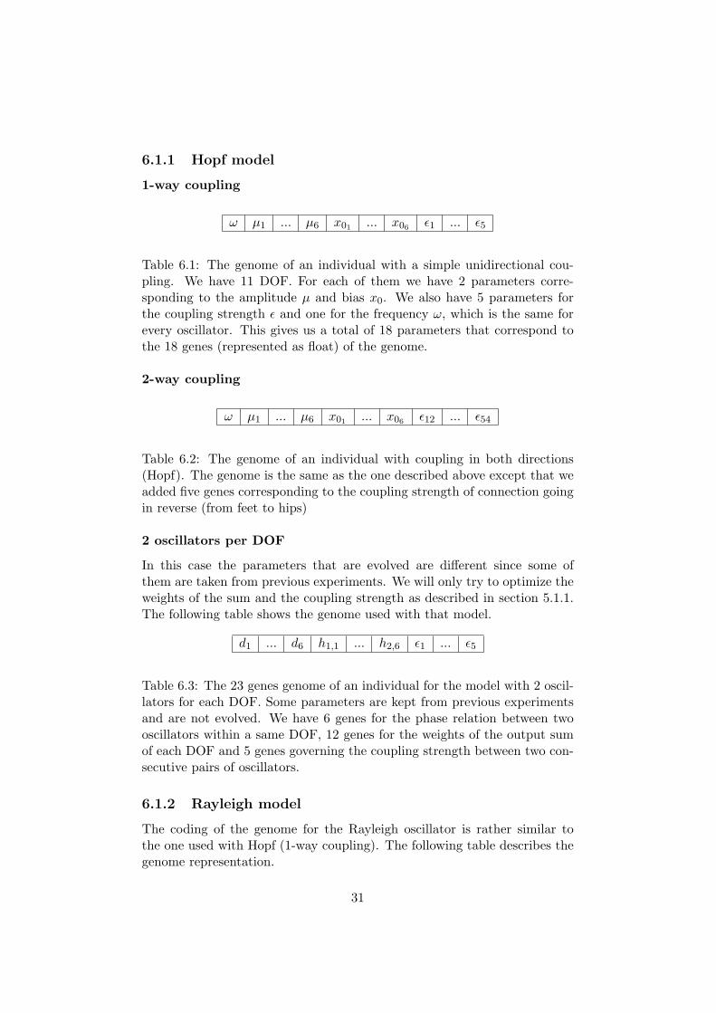
6.1.1 Hopf model

1-way coupling

ω µ1 ... µ6 x01 ... x06 ε1 ... ε5

Table 6.1: The genome of an individual with a simple unidirectional cou-pling. We have 11 DOF. For each of them we have 2 parameters corre-sponding to the amplitude µ and bias x0. We also have 5 parameters forthe coupling strength ε and one for the frequency ω, which is the same forevery oscillator. This gives us a total of 18 parameters that correspond tothe 18 genes (represented as float) of the genome.

2-way coupling

ω µ1 ... µ6 x01 ... x06 ε12 ... ε54

Table 6.2: The genome of an individual with coupling in both directions(Hopf). The genome is the same as the one described above except that weadded five genes corresponding to the coupling strength of connection goingin reverse (from feet to hips)

2 oscillators per DOF

In this case the parameters that are evolved are different since some ofthem are taken from previous experiments. We will only try to optimize theweights of the sum and the coupling strength as described in section 5.1.1.The following table shows the genome used with that model.

d1 ... d6 h1,1 ... h2,6 ε1 ... ε5

Table 6.3: The 23 genes genome of an individual for the model with 2 oscil-lators for each DOF. Some parameters are kept from previous experimentsand are not evolved. We have 6 genes for the phase relation between twooscillators within a same DOF, 12 genes for the weights of the output sumof each DOF and 5 genes governing the coupling strength between two con-secutive pairs of oscillators.

6.1.2 Rayleigh model

The coding of the genome for the Rayleigh oscillator is rather similar tothe one used with Hopf (1-way coupling). The following table describes thegenome representation.

31

ω q1 ... q6 x01 ... x06 ε1 ... ε5

Table 6.4: The genome encoding the parameters of coupled Rayleigh oscil-lators. It is similar to the one used with the Hopf based model with 1-waycoupling, except the parameters qi are responsible for the amplitude of thesignals.

6.1.3 Matsuoka model

We present here the coding of the genome for the parameters used with themodel based on Matsuoka oscillator. The role of the different parametersare described in section 5.1.3.

τ1,i c1 ... c5 x01 ... x03 γ1 ... γ3 α1 ... α4

Table 6.5: The genome encoding the parameters of coupled Matsuoka oscil-lators. Notice that, as τ2 is set to 2τ1, we will not evolve this parameter.

6.2 The algorithm

In this work we use a steady-state algorithm, which means that the popu-lation of two consecutive generations is overlapping.

6.3 The fitness function

The fitness function is certainly the crucial part of the GA as it defines thegoal our individuals will try to reach. The aim of that experiment is to makethe robot walk and not fall. So the fitness function takes into account twoabilities of the robot: the distance it reaches and the time before he falls.The fitness function is described as follow

f = Dz ∗ (T

TotalT ime) (6.1)

where Dz corresponds to the distance (in the z direction) reached by therobot before falling and T is the time before it falls. With this fitness wewill avoid the robot just to stand up without going forward or just fall as faras it can without trying to walk. If the robot does not fall, the simulationstops after a certain time. Also notice that the simulation starts later thanthe oscillators to be sure that all of them are stable.

32

6.4 The GA parameters

The intrinsic parameters of the GA are clearly not the most important partof this experiment. Therefore we used very common values indicated inthe following table. As stopping criterion we set the maximum numberof generations to 150, but for some experiments we ended the algorithmmanually when the fitness no longer increased.

parameter valuepopulation size 100

maxnumber of generation 200probability of mutation 0.25

probability of crossing over 0.9proportion of replacement 0.5

selection scheme Roulette Wheel

Table 6.6: Parameters of the genetic algorithm

Notice that, as we are dealing with real numbers genes, we use a Gaussianmutation operator. The crossing-over operator is only allowed to select acrossing-over point between two genes to make sure that the genome remainscoherent. The selection scheme used here is the roulette wheel selector,which means that the probability of an individual to be kept for the nextgeneration is proportional to its fitness.

33

Chapter 7

Analysis of the results

In this chapter, the different results found with each model will be presentedand compared. As genetic algorithms does not guarantee to find globaloptima, the solutions proposed here might not be the best ones. Thereforeseveral simulations were performed with different initial populations to tryto explore the space search as widely as possible. For each model, we exposethe solution that seemed to be the most efficient and realistic. Notice that,with some models, the GA did not manage to find any good solution in areasonable time.

7.1 Open-loop

7.1.1 Hopf’s oscillator

1-way coupling

After having tuned the intervals of possible values for the CPGs’ parame-ters, quite fast convergence was achieved. A good solution was found afteraround 120 generations. Note that we had to run the algorithm severaltimes to find a good solution as most of the simulations led to the robot tofall after a few steps. This shows us that the GA was far from exploring thewhole solution space.

With that model, the robot managed to walk for about 30 steps beforefalling. The robot did not walk in straight line, it was significantly turningon its left. As the step amplitude was quite large, the robot’s direction wasslightly modified by each step. The contact of the feet and the ground wasalso not very realistic, because it was mostly done on the feet edges. Thewalking speed is approximately 0.25 m/s (cf. figure 7.2). A video of therobot walking is available on the web page of this project1.

1birg.epfl.ch/page58711.html

34

Figure 7.1: Output of the CPG of the best individual found by evolution forthe model based on Hopf oscillators with unidirectional coupling. The bluecurves correspond to the left leg and the red ones to the right leg. This plotonly starts when the simulation begins (the oscillators are started earlier).

Figure 7.2: The robot is walking at 0.25 m/s.

35

The first thing we noticed is that the oscillators reached their limit cyclein approximately 6 periods from any initial conditions. As imposed theleft and right leg were in phase opposition. Another important result, wasthat the resulting amplitude of the oscillators was pretty different from thenatural amplitude because of the strong influence of the coupling. As weonly introduced phase difference of 0 and π, the symmetry of the system(left/right leg) was not really correct since the body’s servo was positivewhen the left leg was ahead and negative when the right leg was ahead. Wealso noticed that the servos that should control the lateral stability (hip1and ankle2) played almost no role in locomotion (cf. figure 7.1).With this model, we managed to make the robot walk for a few steps, butthe solution found was not stable at all and the locomotion is clearly farfrom a realistic walking gait, because of the too simple phase differencesused. To make a more realistic system, phase difference of π/2 and −π/2should have been used.

2-way coupling

With this model we were able to impose phase differences of π/2 and −π/2,which should lead to a more realistic gait than with the previous model. Asexplained above, five extra parameters were added. The search space wasthen significantly enlarged and the impact on the evolution was negative:we did not observe any convergence within a reasonable time.The best result allowed the robot to perform only two or three steps beforefalling. As the evolution for 200 generations took about 12 hours of sim-ulation, we did not perform simulation any further with that model. Theresults obtained will not be analyzed as they are clearly not relevant enough.

2 oscillators per DOF

By adding a second oscillator on each joint, much more complex signals weregenerated and a large variety of signal shape could then be used. Unfortu-nately, the genetic algorithm was unable to find any good solution, even ifthere were less parameters to evolve. One possible explanation of this fact,is that the experiment was based on the best trajectory found with the 1-way Hopf model. As mentioned above, this trajectory does not reflect realbipedal locomotion in terms of phase differences between the different partsof the leg. This trajectory is certainly not robust enough to be modified asit was done by adding a second oscillator.

7.1.2 Rayleigh’s oscillator

As explained above, the next system studied is based on relaxation oscillatorand in particular the Rayleigh oscillator.

36

As expected, signals with a different shape from a simple sinus were pro-duced but just like with the 2-way Hopf model. We ran several simulationsof the GA and none of them seemed to converge significantly even after 200generations. The result on the simulated robot was that it never managedto do more than one step.The possible explanation of such bad performances of the evolution is thatthe possible intervals for the oscillators’ parameters (mainly qi that controlsthe amplitude) are much too large. To generate signal amplitude going from0 to 1, we needed to set an interval for the parameter q roughly comprisedbetween 0 and 10. This caused to enlarge the solution space consequently.In comparison with the Hopf oscillator, the interval for the parameter re-sponsible for the amplitude is only approximately comprised between 0 and1 for the same range of amplitude of the resulting signal.

7.1.3 Matsuoka’s oscillator

Just like with the other models, we tuned the interval of possible values forthe CPG’s parameters by hand. We achieved a relatively fast convergencesince the best individuals were found after approximately 60 generations asshown on figure 7.3. It was not useful to go on with more generations, asmost of the time the fitness was the same, even after 200 generations.

Figure 7.3: Evolution of the fitness function through generations with thegenetic algorithm described above.

The best trajectories found with this model were significantly differentfrom those found with Hopf oscillators. The steps were a bit smaller and

37

allowed the robot to walk in straight line. We managed to make the robotwalk at approximately 0.28 m/s (cf. figure 7.4). We also noticed that thecontact between the robot’s feet and the ground was not perfect due to thetilt of the whole robot. Evolution showed that the Ankle2 servo was a crit-ical part as the contact between feet and ground plays an important role.Computing the position of this servo to make the feet remaining parallel tothe ground was then certainly an important modification in terms of sta-bility. Videos of the robot walking are available on the web page of thisproject2.

Concerning the CPG, we observed that it stabilized slowlier than with theHopf model (10-15 periods). As shown on fig 7.5, the shape of the signalsgenerated by the CPG are different from a simple sinus due to the mutualand self inhibition of the neurons. On this plot we can also see a small phaseshift between the different oscillators along the leg.According to the amplitude of the different servos, we can see that the Hip1joint is more implied in lateral stability than the Ankle2 joint and is there-fore an important DOF to produce a lateral movement that helps the legsgoing from behind to front without touching the ground.An important result is that the oscillator responsible for the body servo playsno role in this solution as its amplitude is null. This might be a problemsince the left an right hip1 servos are coupled to the body servo. It meansthat these two oscillators will not be synchronized with the body oscillatorbecause it does not oscillate. However, the solution found by evolution worksbecause the two hip1 oscillators have the same amplitude, initial conditionsand are in phase. But as soon as there will be perturbations in the system,which could happen when introducing feedback, the two hip1 oscillators willnot stay in phase any longer. To deal with that problem, some modifica-tions were done on the model in order to keep it robust against perturbationswhen adding feedback pathways. These modifications are described in 7.2.

Figure 7.4: The robot is walking at 0.28 m/s.2birg.epfl.ch/page58711.html

38

Figure 7.5: The 11 CPG’s outputs of the best individual found by evolution.The blue curves correspond to the left leg and the red ones to the right leg.This plot only starts when the simulation begins (the oscillators are startedearlier).

The considerations mentioned above only deal with the output of theCPG but not with the real movements produced by the servos during sim-ulation. Figure 7.6 clearly shows a gap between the desired and measuredvalues. Hence, the amplitude of the measured signals are much smaller thanthe desired ones and there is small phase delay between the two curves.These differences occur because the servos’ gains implemented in Webotsare too low and the signal frequency and amplitude we tried to impose

39

were too important. The shape of the measured signal is also different fromthe desire one, hence the trajectories look more like simple sinuses. Wealso noticed, on figure 7.6, there were small perturbations on the measuredtrajectory of the hip2 servos. These perturbations occurred when the feettouched the ground because the friction with the ground created a small re-sistance for the actuators. We will discuss about the servos’ behavior underdifferent frequencies more in details in the next section. Also notice that, atthe beginning of the simulation, the positions of the desired and measuredpositions are very different since the initial conditions of the oscillators werenot set to fit the initial position of the robot.

Figure 7.6: Deviation between the signals we try to impose to the servos(blue line) and the measured movements of the actuators (green line) duringsimulation.

40

7.2 Closed-loop

This section describes the results found when adding feedback pathways tothe open-loop model that gave the best results, as described in section 5.2.We did not try to add feedback to models that use Hopf oscillators andto the model based on Rayleigh oscillators and focus on the model usingMatsuoka oscillators since it gave by far the best results in an open-loopapproach.To find the optimal parameters for the gain of the feedback, we made anexhaustive search for the two parameters Kknee and Khip (cf. figure 7.7)with different values of the time constant τ1, which is inversely proportionalto the frequency of the oscillators output. The results of this search aredescribed in this section.In addition, we tried to test the robustness of our closed-loop model againstsmall perturbations.

7.2.1 Speed adaptation

To modify the walking velocity of the robot, the global frequency of theoscillators was increased. Starting from the best trajectories found withthe open-loop approach, the frequency was modified after three steps of therobots. The frequency was not changed at the beginning of the simulationbecause it had too much impact on the initial conditions. With some fre-quencies the robot started to walk with the wrong leg. Changing the valueof the frequency while the robot was already walking was then a good solu-tion since the aim of this experiment is to modify the walking speed online.Notice that the best open-loop model found was slightly modified for thepurpose of this experiment. First tests of that feedback model showed thatthe feedback pathways generated a small change of the oscillators’ frequen-cies. The consequence of that phenomenon was that the oscillators directlyor indirectly (through coupling) implied in feedback pathways (hip2, knee,ankle1 and ankle2) were no more synchronized with the oscillators that arenot concerned by feedback pathways (body and hip1). In order to avoidthis frequency modification, the coupling between the hip1 and hip2 ser-vos and between the hip2 and knee servos was reinforced (by increasing thecoupling strength) to keep the whole system synchronized. More precisely,every oscillator involved in the feedback pathways were synchronized withthe hip1 oscillator. This could have been done by changing only the couplingstrength between the hip1 and hip2 oscillators. But as the gains ghip andgknee are different, the modification of the hip2 and knee frequency was alsodifferent and thus prevented these two oscillators from synchronizing. Byreinforcing the coupling between these servos, the knee oscillator was thensynchronized with the hip2 oscillator. Also notice that, with the new model,a small phase shift could be seen in the oscillators involved in feedback path-

41

ways (cf. figure 7.9). This slightly changed the phase relation between thehip1 oscillator and the other oscillators. This phase shift is too small to havea real impact on the locomotion since the output of the hip1 oscillator wasstill close to its maximum when both legs are parallel. This is importantsince it allowed the swing leg to go from back to front without hitting theground.As explained above (cf. section 7.1.3), the global coupling model had tobe modified because the two legs were not synchronized since the body os-cillator’s amplitude is null. To deal with that problem, the same oscillatorwas used for the left and right hip1 servos since, in our open-loop model,they are forced to have both the same amplitude, frequency and phase. Toensure that the both legs are synchronized and in phase opposition, phasedifferences of π/2 and −π/2 between the unique hip1 servo and the left andright hip2 servos were respectively imposed. The drawback of this modifica-tion was that the left and right hip1 joints, that mainly control the lateralstability of the robot, always generated the same movements. This could bea limitation since it could be useful to have two distinct signal, for example,if a feedback pathway controlling the lateral stability is added to the system.As the systematic search for system’s gains for one given frequency took ap-proximately 8 hours, we decremented the frequency by steps of 5% of theinitial value of τinitial found with the open-loop model. Figure 7.7 shows theresult of this search

42

Figure 7.7: Velocity of the robot with different gains. Each plot correspondsto a different frequency. Only individuals that do not fall during the simu-lation are considered. The speed of the other ones is set to 0.

43

The gains giving the fastest locomotion for each frequencies are summa-rized in table 7.1.

τ1 frequency [Hz] Khip Kknee velocity [m/s]0.16698 (-0%) 1.66 -0.2 -1.0 0.310.15863 (-5%) 1.76 0.0 -1.4 0.230.15028 (-10%) 1.85 -0.3 -1.4 0.320.14193 (-15%) 1.96 -0.6 -2.2 0.350.13358 (-20%) 2.12 -0.4 -1.3 0.360.12523 (-25%) 2.23 -0.7 -1.0 0.360.11688 (-30%) 2.40 -0.8 -2.0 0.37

Table 7.1: Best gains found for different frequencies and the correspondingspeeds. Notice that τ1 is inversely proportional to the frequency of theoscillator’s output. Typical signals produced by the oscillators with feedbackcan be seen on figure 7.8.

With the systematic search described above, we found optimal gains fordifferent values of the global frequency of the system. As shown on figure7.7, we noticed that, up to 10% of frequency diminution, there were only afew values for the gains that made the robot walk without falling. From 15%to 20% of diminution, we found much more gains that produced stable loco-motion. These values were also roughly distributed within a limited rangeof the gain space we explored. A possible explanation is that, as we had tochange our system when we added feedback pathways, the modified modelcould be better adapted to a range of frequencies going approximately from2 Hz to 2.4 Hz. On the contrary, the model used with the open-loop ap-proach seemed to work better under lower frequency. Also notice that over2.4 Hz, we did not find any values for the gains that did not make the robotfall. As explained, we found values for the gains at given frequencies, butunfortunately we did not manage to find a monotone function that wouldlink the values of Khip and Kknee to the frequency, in order to be able toset the frequency of the system to any value in a continuous interval. Thiswould have allowed us to perform online modifications of the robot’s veloc-ity. We also tried to find gains when the frequency is decreased but evenwith a diminution of 5%, the robot always fell.As shown in table 7.1, we managed to make the robot walk at a speed ofapproximately 0.37 m/s for a frequency of 2.4 Hz, which represents an in-crease of 24% of the velocity found without using feedback pathways.

44

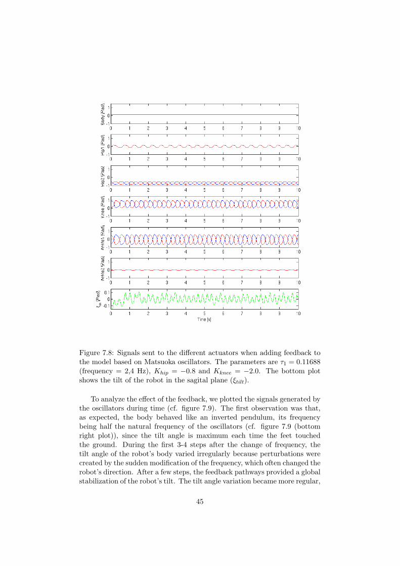
Figure 7.8: Signals sent to the different actuators when adding feedback tothe model based on Matsuoka oscillators. The parameters are τ1 = 0.11688(frequency = 2,4 Hz), Khip = −0.8 and Kknee = −2.0. The bottom plotshows the tilt of the robot in the sagital plane (ξtilt).

To analyze the effect of the feedback, we plotted the signals generated bythe oscillators during time (cf. figure 7.9). The first observation was that,as expected, the body behaved like an inverted pendulum, its frequencybeing half the natural frequency of the oscillators (cf. figure 7.9 (bottomright plot)), since the tilt angle is maximum each time the feet touchedthe ground. During the first 3-4 steps after the change of frequency, thetilt angle of the robot’s body varied irregularly because perturbations werecreated by the sudden modification of the frequency, which often changed therobot’s direction. After a few steps, the feedback pathways provided a globalstabilization of the robot’s tilt. The tilt angle variation became more regular,

45

which made the robot walk in straight line. The effect of the feedback onthe signals produced by the oscillators emphasized a modification of thetrajectories amplitude. This was an expected consequence since we simplyadded a proportional term to the oscillators. As all the best gains Khip

and Kknee found were negative, the amplitude was increased when the tiltangle was negative and decreased when the tilt angle was positive, whichactually produced a modification of the step length. As explained above, thefeedback we used also generated a small phase shift. Also notice that, as theankle1 servo’s position was computed from the position of the hip2 and theknee joints, its value was also modified by the feedback and, as expected,the feet actually stayed roughly parallel to the ground. The amplitude ofthe ankle2 oscillator is also modified since this joint is coupled to the rest ofthe system. Figure 7.10 show a typical example of the compensation doneby the feedback pathways in order to prevent the robot from falling.

46

Figure 7.9: Signals produced by the oscillators with (red) and without (blue)feedback. The feedback pathways slightly modified the amplitude of thesignals. A small phase difference is also produced by the feedback.

47

Figure 7.10: Measured values of the hip2 and knee servos (left and rightlegs) after the modification of frequency (-20%). The frequency is increasedbetween step 1 and 2. The bottom plot corresponds to the value of tilt angleof the robot in the sagital plane. The red curves represent the trajectorieswith feedback (Khip = −0.4 and Kknee = −1.3) and the blue ones corre-spond to model with both gains khip and kknee set to 0. The vertical linecorresponds to the fall of the robot.

Figure 7.10 showed us that, as soon as we modified the frequency, therobot started to lean forward, significantly increasing the mean value of thetilt angle. The consequence on locomotion was that the feet started to hitthe ground earlier, causing bigger perturbations on the measured trajectoriesof the hip1 servos (steps 3 and 4) and the fall of the robot. With feedback,we observed that, as the robot’s tilt angle increased (beginning of step 4),the length of step 4 decreased and thus prevented the foot from hitting theground too abruptly. After that (step 5) the robot tilted backward and thestep length increased. After 3 or 4 more steps the robot’s tilt was stabilizedand it continued walking normally. Also notice that the hip2 servo is muchmore involved in the stabilization process than the knee servo. The impactof the feedback applied on the knee servo is less obvious, but by removing it,the robot always fell. Servos that were indirectly influenced by the feedback(ankle1 and ankle2) also produced modified trajectories, but the impact onstabilization did not seem to be really obvious. On these plots we can alsosee that the feedback produced a small phase shift, which became constantafter 6 or 7 steps.

48

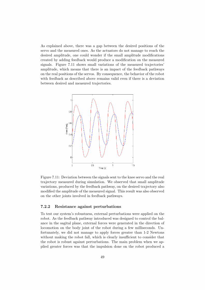
As explained above, there was a gap between the desired positions of theservo and the measured ones. As the actuators do not manage to reach thedesired amplitude, one could wonder if the small amplitude modificationscreated by adding feedback would produce a modification on the measuredsignals. Figure 7.11 shows small variations of the measured trajectories’amplitude, which means that there is an impact of the feedback pathwayson the real positions of the servos. By consequence, the behavior of the robotwith feedback as described above remains valid even if there is a deviationbetween desired and measured trajectories.

Figure 7.11: Deviation between the signals sent to the knee servo and the realtrajectory measured during simulation. We observed that small amplitudevariations, produced by the feedback pathway, on the desired trajectory alsomodified the amplitude of the measured signal. This result was also observedon the other joints involved in feedback pathways.

7.2.2 Resistance against perturbations

To test our system’s robustness, external perturbations were applied on therobot. As the feedback pathway introduced was designed to control the bal-ance in the sagital plane, external forces were generated in the direction oflocomotion on the body joint of the robot during a few milliseconds. Un-fortunately, we did not manage to apply forces greater than 1-2 Newtonswithout making the robot fall, which is clearly insufficient to consider thatthe robot is robust against perturbations. The main problem when we ap-plied greater forces was that the impulsion done on the robot produced a

49

too fast tilt of the robot in the direction of walking and the robot was unableto react quickly enough to the sudden modification of the body’s tilt. Byconsequence, we concluded that the gains of the feedback pathways were toolow for that kind of perturbation and a different model should be used todeal with both perturbations and speed adaptation.

50

Chapter 8

Conclusion

8.1 The project

The study of bipedal locomotion is quite a new field that is only a few tenyears old. However, researches done on this subject show the huge amountof different possibilities there are to try to imitate the incredibly complexhuman gait.Inspired from biological considerations, we tried, in this work, to exploreand analyze a few models using oscillator based CPGs as controllers for asimulated biped robot. Artificial evolution was also used to optimize theparameters of the oscillators, in order to generate an efficient locomotion.In the first part of this project, several models of oscillators were artificiallyevolved. We firstly used Hopf oscillators with different types of couplingbetween them and achieved a walk of about 30 steps with a velocity of ap-proximately 0.25 m/s. As this solution was found with the simplest couplingmodel we tested, this first experiment also showed that it was difficult tomake the genetic algorithm converge in a reasonable time with more complexmodels. Most of the time, extra parameters added for more sophisticatedcoupling models led to a important enlargement of the search space that ouralgorithm did not manage to explore efficiently. The same problem occurredwhen we used a relaxation oscillator. In this case, the range of possible pa-rameters was also too large to see any interesting solution emerging fromartificial evolution.We also studied Matsuoka oscillators, which are based on the mutual inhi-bition of two coupled neurons and are often used for bio-inspired neuronalmodels. This model gave by far the best results and the genetic algorithmconverged easily. The best solution found allowed the robot to walk indefi-nitely at a speed of approximately 0.28 m/s and with a rather realistic gait.This last model was then improved by adding feedback pathways in orderto be able to increase the speed of the locomotion by changing the globalfrequency of the system. This was done by using the tilt angle of the body

51

in the sagital plane to modify the trajectories of the hip2 and knee servos.This feedback pathway proved to be quite efficient since we managed to in-crease the velocity of the robot of about 25% (0.37 m/s) by increasing thefrequency by 30%. The main impact of the feedback on locomotion wasthat it modified the trajectories of the hip1 servos, preventing the robotfrom falling forward when the frequency is increased.We also tried to apply external perturbations on the robot in the direction ofwalking. Unfortunately, the robot was only able to remain stable after verysmall perturbations (1-2 Newtons). In addition, this model did not allow usto modify the speed of the robot online by changing frequencies comprisedin a continuous range.In this work, we have demonstrated that a rather simple feedback pathwaymodel clearly improved the locomotion when the frequency is increased. Fi-nally, this project has opened the way to many possible upgrades of themodel since we only explored a small part of the possibilities offered bybio-inspired artificial locomotion.

8.2 Further work

This work explored different model of oscillators and couplings giving vari-ous results. A lot of other oscillators could obviously be used, particularlyoscillators able to generate more complex signals closer to human locomo-tion could be of interest. The Matsuoka oscillator gave good results andshould be studied more deeply.In this study only one kind of feedback pathways was used. It would be use-ful to implement more complex models like a feedback pathway that controlsthe lateral stability of the robot or a feedback using the touch sensors of therobot’s feet. One could also try to deal with more complex perturbationssuch as lateral wind, slopes or irregular ground. A more difficult but ob-viously important development would be to be able to control the robot’sdirection during simulation. The solutions found in this work should alsobe tested on the real Hoap2 robot.

52

Bibliography

[1] Christopher L. Vaughan. Theories of bipedal walking: an odyssey. Jour-nal of Biomechanics, Volume 36, Issue 5, November 2000.

[2] A. J. Ijspeert. Vertebrate locomotion. The handbook of brain theory andneural networks. 649:654. MIT Press. 2003.

[3] Jonas Buchli, Auke Jan Ijspeert. Distributed central pattern genera-tor model for robotics application based on phase sensitivity analy-sis.Biologically Inspired Approaches to Advanced Information Technol-ogy: First International Workshop, BioADIT 2004, Lecture Notes inComputer Science, Springer, 2004

[4] McGeer T. Passive dynamic walking. International Journal of RoboticsResearch. 9(2):62-82. 1990.

[5] Collins S. H., Ruina, A. A bipedal walking robot with efficient andhuman-like gait. In Proc. IEEE International Conference on Roboticsand Automation. 2005.

[6] F. Asano, M. Yamakita, N. Kamamichi, Z-W Luo. A novel gait gener-ation for biped walking robots based on mechanical energy constraint.IEEE transaction on robotics and automation. vol. 20, no 3. 2004.

[7] M. Vukobratovic, B. Borovac, D. Surla and D. Stokic. Biped locomo-tion: dynamics, Stability, Control and Applications. Springer. 1990.

[8] J. Pratt, P. Dilworth, G. Pratt. Virtual model control of a bipedal walk-ing robot. Proceeding of the IEEE International Conference on Robotics& Automation. 193-198. 1997.

[9] S. Grillner. Control of motion in bipeds, tetrapods and fish. In V.Brooks (Ed.), Handbook of Phisiology, The Nervous System, 2, MotorControl . 1179-1236. American Physiology Society. Bethesda. 1981.

[10] G. Taga. Emergence of bipedal locomotion through entrainment amongthe neuro-musculo-skeletal system and the environment. PHYSIKA D,75:190-208. 1994

53

[11] G. Taga. A model of the neuro- musculo-skeletal system for anticipatoryadjustment of human locomotion during obstacle avoidance. BiologicalCybernetics. 78(1):9-17. 1998

[12] A. J. Ijspeert. A connectionist central pattern generator for the aquaticand terrestrial gaits of a simulated salamander.Biological Cybernetics.84(5):331-348. 2001

[13] A. J. Ijspeert, J-M Cabelguen. Gait transition from swimming to walk-ing: investigation of salamander locomotion control using nonlinear os-cillators. Proceeding of adaptive motion in animals and machines. 2003

[14] A. J. Ijspeert, J. Hallam, D. Willshaw. Evolving swimming controllersfor a simulated lamprey with inspiration from neurobiology. Adaptivebehavior. 7(2):151-172. 1999.

[15] S. Strogatz. Non-linear Dynamics and Chaos, Addison Wesley Publish-ing Company. 1994.

[16] A. Pikovsky, M. Rosenblum, J. Kurths. Synchronization, A universalconcept in non-linear sciences. Cambridge University Press. 2001.

[17] K. Matsuoka. Sustained oscillations generated by mutually inhibitingneurons with adaptation. Biol. Cybern.. 52:367-376. 1985

[18] K. Matsuoka. Mechanisms of frequency and pattern control in the neu-ral rhythm generators. Biol. Cybern.. 56:345-353. 1987.

[19] M. M. Williamson. Robot arm control exploiting natural dynamics.thesis. Massachusetts Institute of Technology. 1999.

[20] WEBOTS. www.cyberbotics.com. Commercial Mobile Robot Simula-tion Software.

[21] P. Cominoli, Development of a physical simulation of a real humanoidrobot. Master’s thesis. 2004-2005.

[22] Galib. lancet.mit.edu/ga/. A C++ Library of Genetic Algorithm Com-ponents.

[23] Fujitsu HOAP 2. www.automation.fujitsu.com/en/products/products09.html.Humanoid Robot HOAP-2.

54