Evidence Suppression by Prosecutors: Violations of the Brady Rule*

Andrew F. Daughety and Jennifer F. Reinganum**Department of Economics and Law School

Vanderbilt University

August 2016revised: January 2018

* We thank Giri Parameswaran and Alan Schwartz, along with participants in the Warren F.Schwartz Memorial Conference, Georgetown University Law Center; the Law and EconomicsTheory Conference VI, NYU Law School; the Winter 2017 NBER Law and Economics Workshop;the University of Bonn BGSE Workshop and Micro Theory Seminar; the University of MannheimLaw and Economics Forum; the American Law and Economics Association 2017 Meetings;Northwestern University Pritzker School of Law; Queen’s University Smith School of Business; andthe Hong Kong University of Science and Technology Conference on Law and Economics forcomments on earlier versions. Finally, we also thank three anonymous referees and the EditorWouter Dessein for constructive comments on a previous version.

** andrew.f.daughety@vanderbilt.edu; jennifer.f.reinganum@vanderbilt.edu

Evidence Suppression by Prosecutors: Violations of the Brady Rule

Abstract

We develop a model of individual prosecutors (and teams of prosecutors) to address theincentives for the suppression of exculpatory evidence. Our model assumes that each individualprosecutor trades off a desire for career advancement (by winning a case) and a disutility forknowingly convicting an innocent defendant. We assume a population of prosecutors that isheterogeneous with respect to this disutility, and each individual’s disutility rate is their own privateinformation. A convicted defendant may later discover exculpatory information; a judge will thenvoid the conviction and may order an investigation. Judges are also heterogeneous in theiropportunity costs (which is each judge’s private information) of pursuing suspected misconduct. We show that the equilibrium information configuration within the team involves concentration ofauthority about suppressing/disclosing evidence. We further consider the effect of angst aboutteammate choices, office culture, and the endogenous choice of effort to suppress evidence.

1. Introduction

In the United States, Brady v. Maryland (1963) requires that prosecutors disclose exculpatory

evidence favorable to a defendant; not disclosing is a violation of a defendant’s constitutional right

to due process. The Brady Rule requires disclosure of evidence “material” to guilt or punishment,

where evidence is material if its disclosure could change the outcome. In a series of judicial

decisions this was extended to include: 1) evidence that can be used to impeach a witness; 2)

evidence favorable to the defense that is in the possession of the police; and 3) undisclosed evidence

that the prosecution knew, or should have known, that their case included perjured testimony (see

Kozinski, 2015, and Kennan, et. al., 2011). One standard rationale for this rule is that the

prosecution (i.e., the state) has considerably more power and greater access to resources (e.g., the

police as an investigative tool) than the typical criminal defendant. An authority on prosecutorial

misconduct1 has observed that “... violations of Brady are the most recurring and pervasive of all

constitutional procedural violations, with disastrous consequences ...” (Gershman, 2007, p. 533).

As an example of a collection of Brady violations, in 1999 John Thompson, who had been

convicted, separately, of armed robbery and of murder and had been on death row in Louisiana for

fourteen years, was within four weeks of his scheduled execution when a private investigator

stumbled across blood evidence relevant to Thompson’s defense in the armed robbery, which

prosecutors in the Orleans Parish District Attorney’s Office had suppressed.2 Justice Ginsburg’s

1 See Gershman (2015) for an extensive discussion of the different forms of prosecutorial misconduct. Theseinclude (but are not limited to) nondisclosure of evidence, misconduct in the grand jury, abuse of process, misconductin plea bargaining, in jury selection, in the presentation of evidence, in summation, and at sentencing.

2 Thompson was (strategically) prosecuted sequentially for these two unrelated crimes. This was done so thata conviction for the armed robbery would weaken his defense in the murder prosecution; he was convicted of bothcrimes. After being found innocent of murder in a retrial, Thompson sued Harry Connick, Sr. in his capacity as DistrictAttorney for the Parish of Orleans. At trial, Thompson won $14 million dollars compensation from the Parish, but theU.S. Supreme Court in a 5-4 decision later voided the award. The description here and elsewhere in the paper is takenfrom a combination of the majority opinion authored by Justice Thomas and, especially, the dissenting opinion authoredby Justice Ginsburg in Connick v. Thompson, 563 U.S. 51 (2011).

2

dissent in Connick v. Thompson details how all of the aforementioned aspects of Brady protection

were violated in Thompson’s cases.3 Judge Alex Kozinski, a past Chief Judge on the U.S. Ninth

Circuit Court of Appeals, has argued that “There is an epidemic of Brady violations abroad in the

land” (United States v. Olsen, 737 F.3d 625, 626; 9th Cir. 2013), and listed a number of federal cases

involving Brady violations. The few studies on prosecutorial misconduct that exist have found

thousands of instances of various types of prosecutorial misconduct, including many Brady

violations (see Kennan et. al., 2011).

1.1 This Paper

Motivated by the problem of suppression of exculpatory evidence, we develop a model of

individual prosecutors and prosecutorial teams. Teams are employed to share effort, to capture the

benefit of diverse talents, and to train less-experienced prosecutors. We intentionally abstract from

these legitimate benefits of teams, so as to focus on an illegitimate activity: the choice by

prosecutors to suppress evidence in violation of a defendant’s Brady rights, which is facilitated by

the (endogenously-determined) compartmentalized receipt of exculpatory evidence.

Our model assumes that each individual prosecutor trades off a desire for career

advancement (by winning a case) and a disutility for knowingly convicting an innocent defendant

by suppressing exculpatory evidence. We assume a population of prosecutors that is heterogeneous

with respect to this disutility, and each individual’s disutility is their own private information. A

convicted defendant may later discover exculpatory evidence. To simplify matters, we assume the

discovered evidence is brought to a court where a judge will then void the conviction and may order

3 The blood evidence was artfully hidden; in the murder case, a witness’s description was substantially modifiedto resemble Thompson and another “witness” (who better fit the original witness’s description) provided perjuredtestimony against Thompson.

3

an investigation of the prosecutors from the case, depending upon her (privately known) disutility

of pursuing an investigation.4 If a prosecutor is found to have violated the defendant’s Brady rights,

the prosecutor is penalized. The anticipated game between the prosecutors and the reviewing judge

is the main consideration of this paper.

1.2 Related Literature

Economists have developed an extensive literature on the incentives for agents (usually

sellers in a market) to reveal information (see Dranove and Jin, 2010, for a recent survey of the

literature on the disclosure of product quality). A standard result concerning the costless disclosure

of information is “unraveling” wherein an informed seller cannot resist disclosing the product’s true

quality to avoid an adverse inference (see Grossman, 1981, and Milgrom, 1981). Complete

unraveling does not occur if disclosure is costly or if there is a chance the seller is uninformed.5

Possibly closest to our paper is Dye (2017); in both Dye’s paper and our paper, an agent may

or may not possess private information but, if he has it, he has a duty to disclose it. Failure to

disclose may be detected and entails a penalty. In Dye, the private information is about the future

value of an asset, which is priced in the stock market. After the pricing stage, a fact-finder audits

the agent with an exogenous probability; the penalty for failing to disclose is consistent with

securities law. Our model differs in that our agent also has a moral cost associated with the

4 In reality, prosecutorial accountability is addressed via a variety of approaches in the different states; forexample, in North Carolina cases referred to the State Bar (a government agency) are handled by a separate (civil) court,while in New York suits proceed via private lawsuits within the usual appeals system. We have simplified the responseof the legal system to a reviewing judge ordering an investigation; for more institutional detail, see Keenan, et. al., 2011.

5 Matthews and Postlewaite (1985) and Shavell (1994) analyze an agent who chooses whether to acquireinformation and whether to disclose it. They focus on voluntary versus mandatory disclosure and find that mandatorydisclosure may discourage information acquisition. Garoupa and Rizzolli (2011) apply this finding to the Brady rule. They argue that a prosecutor may be discouraged from searching for additional evidence (which might be exculpatory)if its disclosure is mandatory, and they show that this could harm an innocent defendant.

4

consequences of his failure to disclose, and there is an endogenous investigation decision made by

a judge. Furthermore, we extend the one-prosecutor model to consider a team of prosecutors that

can organize itself in terms of the receipt and disclosure of exculpatory evidence.

Our prosecutor’s payoff function includes aspects of career concerns and moral concerns

about causing the conviction of a defendant he knows to be innocent. The theoretical literature on

plea bargaining and trial involves several different prosecutorial payoff functions that place a

varying amount of weight on these two aspects. Landes (1971) assumes the prosecutor maximizes

expected sentences, whereas Grossman and Katz (1983), Reinganum (1988), Bjerk, (2007), and

Baker and Mezzetti (2011) employ objectives that approximate social welfare. Daughety and

Reinganum (2016) assume that a prosecutor benefits from longer expected sentences, but endures

informal sanctions (such as loss of an election) from members of the community who might think

the prosecutor is sometimes convicting the innocent and other times allowing the guilty to go free.

Empirical work on prosecutorial objectives finds evidence of career concerns, but also a

preference for justice. Glaeser, Kessler, and Piehl (2000) find that some federal prosecutors are

motivated by reducing crime while others are primarily motivated by career concerns. Boylan and

Long (2005) find that higher private salaries are associated with a higher likelihood of trial by

assistant U.S. attorneys (trial experience may be valuable in a subsequent private-sector job).

Boylan (2005) finds that the length of prison sentences obtained is positively related to the career

paths of U.S. attorneys. McCannon (2013) and Bandyopadhyay and McCannon (2014) find

evidence that prosecutors up for reelection seek to increase the number of convictions at trial.

1.3 Plan of the Paper and Overview of the Results

In all versions of the model we have one reviewing judge (J, whose type is her disutility of

5

an investigation; this is J’s private information) and one defendant (D, whose type is either guilty

or innocent; this is D’s private information). In Section 2 we develop a one-P model, wherein P’s

disutility of convicting an innocent D (P’s type) is his private information. We first characterize the

Bayesian Nash Equilibrium (BNE) between the prosecutor and the judge, wherein a subset of P-

types will suppress evidence and a subset of J-types will conduct an investigation.

Section 3 expands the analysis to consider two Ps (each with his own private information as

to type) and examines two models, one wherein only one P can observe whether exculpatory

evidence exists (we will refer to this as the “21” configuration to capture that there are two Ps but

only one is aware of any exculpatory evidence) and one wherein both Ps automatically learn whether

such evidence exists (this is the “22” configuration). We find that the set of P-types who would

prefer to suppress the evidence may be larger in the 22 configuration. However, the equilibrium

probability of suppression in the 22 configuration is lower than in the 21 configuration.

In Section 4 we endogenize the choice of configuration within the team and find that

(assuming J cannot observe the choice) the equilibrium configuration is 21. In Section 5 we

consider the possibility that: 1) a P may suffer angst due to suppression by a teammate; 2) a P may

be rewarded or punished by a teammate (or others in the office) for either disclosing or suppressing;

and 3) costly effort may be expended to reduce D’s likelihood of discovering exculpatory evidence.

Section 6 provides a summary and a discussion of policies intended to improve information flows

and to reduce prosecutorial misconduct.

2. Model Set-up, Notation, and Analysis for the Single-Prosecutor Model

In this section, we will describe the model and results for the case of one prosecutor facing

one defendant and one reviewing judge. P and D have access to (different) evidence-generating

6

processes in the case for which P is prosecuting D. In either case, a party may observe exculpatory

evidence (denoted as E) or not observe exculpatory evidence (denoted as φ). We assume that P’s

opportunity to observe E occurs just prior to the trial, whereas D’s opportunity to observe E occurs

after the trial. Note that this means that if P does observe E, but suppresses this information, then

D may never become aware of E (D may only observe φ). Alternatively, if P does not observe E

(i.e., P observes φ), then E may still exist and D might later observe it.

Let the prior probability of innocence be denoted λ; that is, λ / Pr{D is I}, where we

assume λ 0 (0, 1). The evidence-generating processes are based on D’s true type, G (guilty) or I

(innocent), which is D’s private information. Let γ / Pr{P observes E | D is I}, so 1 - γ = Pr{P

observes φ | D is I}. Similarly, let η / Pr{D observes E | D is I}, so 1 - η = Pr{D observes φ | D is

I}. Both γ and η are also assumed to be positive fractions.6 The simplest way to interpret these

probabilities is that E exists whenever D is innocent, although it may not be found (observed) by

either P or D.7 Moreover, we assume that if D is G, then no exculpatory evidence exists so that

neither P nor D will ever observe E; they will each observe φ with certainty. Finally, we assume that

without E, D will be convicted, whereas with E, D will be found innocent. Thus, exculpatory

evidence in our analysis is “perfect” in the sense that it is absolutely persuasive and clearly material.8

Before the trial begins, P has an opportunity to report (disclose) the receipt of exculpatory

6 Although we need not impose any ordering on γ and η, it is typically thought that the prosecution generallyhas more resources that can be brought to bear on finding evidence than does the defendant, so a typical ordering wouldbe γ > η. In Section 5 we allow P to influence the size of η via suppression effort.

7 More complex lotteries could be specified (i.e., when D is I, E may or may not exist, and may or may not befound when it does exist), but this generates additional complexities without accompanying benefits.

8 In reality, exculpatory evidence may not be perfect, so it may only reduce the chance of conviction. Furthermore, imperfect exculpatory evidence may be observed even though D is of type G. Consideration of imperfectexculpatory evidence would considerably complicate the model (injecting a variety of additional parameters andinference conditions) and distract from our focus on the incentives for prosecutors to limit the distribution of E withina team and to suppress the evidence from D.

7

evidence. Let θ 0 {E, φ} denote P’s true evidence state (which is P’s private information), and let

r 0 {E, φ} denote P’s reported evidence state. Then the pair (r; θ) = (E; E) implies that P disclosed

E when he observed E, whereas (r; θ) = (φ; E) implies that P failed to disclose E when he observed

E (because he reported having observed φ). We assume that E is “hard” evidence, so it cannot be

reported when it was not observed; that is, when P observes φ, then he must report φ.

We assume that P obtains a payoff of S when D is convicted, where S reflects career

concerns such as internal advancement or improved outside opportunities. However, P also suffers

a loss of τ if D is falsely convicted due to P’s suppression of exculpatory evidence, where τ is a

random variable that is distributed according to F(τ), with density f(τ) > 0, on [0, 4); that is, τ is P’s

type. Thus, some prosecutor types (τ-values) would prefer a false conviction to none at all, whereas

others would prefer no conviction to being responsible for a false one.9

As stated earlier, if P does not disclose any exculpatory evidence, we assume that the

evidence provided at trial is sufficient to convict D. However, following D’s conviction, it is

possible that D will discover exculpatory evidence (if D is truly innocent). In this case, we assume

that D will go to court and have her conviction overturned by a reviewing judge and P loses the

amount S associated with a conviction (independent of whether P suppressed E); we assume that P

continues to incur the loss τ if he suppressed E. J also has the opportunity to investigate the

prosecutor’s behavior, which could have been appropriate (if P did not observe E) or inappropriate

(if P observed E but reported φ). Assume that when an investigation verifies P’s failure to disclose,

the judge receives a payoff of V (e.g., many judges run for office or for retention and this sort of pro-

9 For simplicity we have confined P’s private information to one aspect of his payoff (the disutility τ). Alternatively, we could view τ as commonly known and let S be P’s private information. This yields equivalent results.

8

social behavior can elicit electoral support) and P receives a penalty of k.10 Further, J faces a

disutility c of conducting an investigation, which might involve resource or opportunity costs due

to holding hearings, distaste for confronting colleagues in the judicial process (regardless of

outcome, J will probably work with them again), along with potential retaliation from prosecutors.

As an example of prosecutorial retaliation against a judge who attempts to enforce the Brady

rule, consider the following incident. In a capital-murder case in Orange County, Scott Dekraai was

convicted (in part) on the basis of testimony by a jailhouse informant. As described in Kozinski

(2015, p. xxvi), the defense challenged the informant and:

“... Superior Court Judge Thomas Goethals ... eventually found that the Orange CountyDistrict Attorney’s office had engaged in a ‘chronic failure’ to disclose exculpatory evidencepertaining to a scheme run in conjunction with jailers to place jailhouse snitches known tobe liars near suspects they wished to incriminate, effectively manufacturing falseconfessions. The judge then took the drastic step of disqualifying the Orange CountyDistrict Attorney’s office from further participation in the case.”

Subsequently, the Orange County DA’s office made use of peremptory challenges to remove Judge

Goethals from significant cases they were prosecuting. According to Saavedra (2016), “Appellate

justices ruled Monday that the Orange County District Attorney’s Office can disqualify Superior

Court Judge Thomas Goethals from 46 murder cases, though the justices also said the practice is

abusive and disruptive of the court system.”

J’s disutility c from investigating is her private information (i.e., her type) and is distributed

according to H(c), with density h(c) > 0, on [0, 4).11 Thus, a judge with a sufficiently low value of

10 See Gershman (2015), Chapter 14 for a discussion of sanctions for prosecutorial misconduct. For example,k could include fines or jail time (California has recently passed a law in ths regard) or loss of law license, as well asreputational losses. Note that it is also straightforward to incorporate a reputational loss due simply to being investigated(i.e., even if P is not found to have suppressed evidence).

11 As with P’s type, we have confined J’s private information to one aspect of her payoff (the disutility c). Alternatively, we could view c as commonly known and let V be J’s private information. This yields equivalent results.

9

c will investigate, whereas one with a sufficiently high value of c will overturn D’s conviction but

will forego investigating P.12 An investigation may fail to verify P’s suppression; let μ denote the

positive probability that the investigation verifies P’s failure to disclose material exculpatory

evidence that was in P’s possession. We assume there are no “false positives;” that is, an

investigation never concludes that P failed to disclose E when P actually observed φ.

2.1. Timing of Moves

The previous discussion implies the following information structure and timing of moves.

1. Nature determines whether D is G (guilty) or I (innocent), and reveals this only to D.

2. Nature determines whether P observes E or φ, and P’s type τ; these are revealed only to P.

3. P reports E or φ. If P reports E, then D is exonerated and the game ends. If P reports φ, then

D is convicted; P obtains S but pays τ if P had observed E.

4. If D is convicted, then Nature determines whether D observes E or φ. If D observes φ, then the

game ends. If D observes E, then D provides E to J and D is exonerated; P loses the payoff

S previously obtained, but if P suppressed E, then he continues to bear the disutility loss τ.

5. Nature determines J’s type c; this is revealed only to J. J decides whether to investigate P. If

J decides not to investigate P, then the game ends. If J investigates P, then if P is not found

to have suppressed E, the game ends; if P is found to have suppressed E, then P’s penalty is

k, J obtains V, and the game ends.

2.2. Payoff Functions and Decisions for P and J

Using the notation and timing specification described above, we can construct payoffs and

analyze decisions for P and J. First, we consider the problem facing P. Let πP(r; θ, τ) denote P’s

12 We have assumed that J cannot credibly commit to an investigation policy. Since J’s type is her privateinformation, it would be difficult to verify whether she had adhered to any announced policy.

10

expected payoff from reporting r when he observed θ; this payoff is indexed by P’s type, τ. We

assume that P’s career concerns are such that he gains S from every conviction, but loses τ only

when he knows he has caused a false conviction by suppressing exculpatory evidence.13

Thus, πP(E; E, τ) = 0: when P observes and discloses E, then D is not convicted. When P

observes φ, he must also report φ. However, D may subsequently observe E, in which case the

conviction is reversed but, since P acted appropriately, he faces no sanction (recall, we assume there

are no “false positives” when J investigates P) and since he did not create a harm by suppressing E,

he bears no disutility loss τ. Thus, πP(φ; φ, τ) = S - Pr{D observes E | P observed φ}S. P’s posterior

belief Pr{D observes E | P observed φ} = ηλ(1 - γ)/[1 - λ + λ(1 - γ)].14 Therefore,

πP(φ; φ, τ) = S{1 - ηλ(1 - γ)/[1 - λ + λ(1 - γ)]}.

Finally, when P observes E, he knows that D is innocent. Failure to disclose E (that is, a report of

φ) means that P incurs a disutility loss equal to his type τ; this disutility persists even if the

conviction is eventually reversed. Moreover, even if P suppresses E, there is a chance that D will

discover it herself. In this case, P will not only lose the value of the conviction and incur the

disutility loss for harming D, but he will also face the risk of investigation and possible sanction.

Given the timing, J decides whether to investigate only when D provides evidence E and P did not

previously report E; thus, when deciding whether to suppress an observation of E, P must form a

conjecture about the likelihood that J will investigate. Let ρ^ denote P’s conjectured likelihood of

investigation, when P reported φ and D provided the exculpatory evidence E. Thus πP(φ; E, τ) = S -

13 Some innocent Ds may be convicted due to undiscovered exculpatory evidence, but P can rationalize theseas good (or at least untainted) convictions, as he was unaware of E and took no action to suppress it.

14 The denominator represents the ways that P could observe φ (D is G, which happens with probability 1 - λ,or D is I but P did not observe E, which happens with probability λ(1 - γ)). Thus λ(1 - γ)/[1 - λ + λ(1 - γ)] represents P’sposterior assessment that D is innocent, given P observed φ; η is the probability that an innocent D will discover E.

11

τ - Pr{D observes E | P observed E}(S + kμρ^). Since a P that observed E knows that D is innocent,

P’s posterior Pr{D observes E | P observed E} = η. Therefore πP(φ; E, τ) = S(1 - η) - τ - ηkμρ^.

We can now define a strategy for P and a best response for P to his conjecture about J’s

likelihood of investigation.

Definition 1. A strategy for P is a choice of report, conditional on P’s observation of θ andP’s type τ; that is, r(θ, τ) 0 {E, φ}. Note that in order to report (disclose) E, P must actuallyhave observed E, so r(φ, τ) = φ is imposed; we need only consider r(E, τ) . A best responsefor P to his conjecture ρ^ is the r 0 {E, φ} that maximizes πP(r; E, τ).

It is clear that P will choose to suppress observed exculpatory evidence if:

πP(φ; E, τ) = S(1 - η) - τ - ηkμρ^ > πP(E; E, τ) = 0.

This occurs if and only if τ < t(ρ^), where t(ρ^) / max {0, S(1 - η) - ηkμρ^}. The following lemma

characterizes the set of P-types that will suppress exculpatory evidence.15

Lemma 1. If P observes E, P’s best response is: BRP(ρ^ ; τ) = φ if τ < t(ρ^) and BRP(ρ^; τ) =E if τ > t(ρ^), where t(ρ^) / max {0, S(1 - η) - ηkμρ^}.

Lemma 1 states that a P of type τ who observes E and conjectures that J will investigate with

probability ρ^ will optimally follow a threshold rule with respect to suppression: suppress evidence

if τ is sufficiently low and otherwise disclose the evidence.

Next, consider the problem facing J. J makes a decision in this model only if P did not report

E prior to D’s conviction, and D subsequently discovered E following her conviction. J will reverse

D’s conviction but J can also decide whether to investigate P’s behavior to ascertain whether P

suppressed evidence of D’s innocence. Let d 0 {1, 0} denote this decision, where d = 1 means that

J investigates and d = 0 means that J does not investigate. To make this decision, J must construct

15 Our specification of P’s best response assumes an indifferent P-type discloses E; since there is a continuumof types, it would not affect our results if an indifferent P-type was assumed to suppress E. However, for someparameters and conjectures, it may be that every τ > 0 strictly prefers to disclose (i.e., suppression is strictly deterred),in which case the constraint that t(ρ^) > 0 binds and we want τ = t(ρ^) = 0 to belong to the set of types that disclose.

12

a posterior probability that P actually had observed E but failed to disclose it. This requires J to

conjecture a threshold, denoted t^, such that all P types with τ < t^ are expected to report φ when they

observe E. Since D provided J with the exculpatory evidence E, D is now known to be innocent.

Thus, J’s posterior assessment that P lied when he reported φ is γF(t^)/[1 - γ + γF(t^)].16

Recall that: 1) J receives a value V when her investigation reveals and sanctions a P that has

suppressed exculpatory evidence; 2) an investigation verifies P’s suppression with probability μ; and

3) an investigation entails a disutility for J of c, which is drawn from the distribution H(c). Then a

J of type c has an expected payoff of πJ(d; c), where:

πJ(1; c) = VμγF(t^)/[1 - γ + γF(t^)] - c and πJ(0; c) = 0.

Hence, we define parallel notions of strategy and best response for J as follows.

Definition 2. A strategy for J is a decision to investigate or not (in the event that D providesE and P’s prior report was φ), conditional on J’s type c; that is, d(c) 0 {1, 0}. A bestresponse for J to her conjecture t^ is d(c) 0 {1, 0} that maximizes πJ(d; c).

It is clear that πJ(1; c) = VμγF(t^)/[1 - γ + γF(t^)] - c > πJ(0; c) = 0 whenever c < VμγF(t^)/[1 -

γ + γF(t^)]. The following lemma characterizes the set of J-types that will investigate P on suspicion

of suppressing exculpatory evidence.

Lemma 2. If P reported φ and D later provided E, J’s best response is: BRJ(t^; c) = 1 if c <VμγF(t^)/[1 - γ + γF(t^)] and otherwise BRJ(t^; c) = 0.

Lemma 2 states that a J faced with a convicted D submitting exculpatory evidence, when P

previously reported φ, and who conjectures that the threshold rule for P was to suppress if τ < t^, will

optimally follow her own threshold rule with respect to investigation: investigate if her disutility

16 The denominator consists of all the ways that P could have reported φ (given that we now know that D isinnocent). P would have reported φ if he truly did not observe E (which happens with probability 1 - γ) or if he didobserve E, but his type fell below the threshold for disclosure (which happens with probability γF( t^)). Thus, the shareof φ-reports that are due to evidence suppression is the ratio γF( t^)/[1 - γ + γF( t^)].

13

of doing so, c, is sufficiently low and otherwise do not investigate.

2.3. Equilibrium

Lemmas 1 and 2 characterize P’s and J’s best response functions. However, it will be more

intuitive to work with the following functions which summarize the best response behavior of,

respectively, P and J (and we use a superscript BR to capture this):

tBR(ρ) / S(1 - η) - ηkμρ; (1)

ρBR(t) / H(VμγF(t)/[1 - γ + γF(t)]). (2)

The function tBR(ρ) represents the minimum threshold level of τ consistent with disclosure, given

any conjectured probability ρ of J ordering an investigation. The function ρBR(t), which (from the

definition of H) is always less than one, represents the probability that a randomly-drawn judge will

decide to investigate, given any conjectured threshold t for disclosure.

Definition 3. A Bayesian Nash Equilibrium (BNE) is a pair (t*, ρ*), such that t* = max {0, tBR(ρ*)} and ρ* = ρBR(t*).

Notice that equation (2) above implies that if t* were 0 then ρ* would be 0 as well, but then

equation (1) above implies that t* > 0. Therefore, it must be that t* > 0. Basically, if J does not

expect any P-types to suppress exculpatory evidence, then J will never investigate, but then some

P-types will choose suppression. Thus, we know the equilibrium occurs along the function tBR(ρ).

Proposition 1. There is a unique BNE, (t*, ρ*), where t* 0 (0, S(1 - η)) and ρ* 0 (0, 1), givenby the pair of equations:

t* = S(1 - η) - ηkμρ*; (3)

ρ* = H(VμγF(t*)/[1 - γ + γF(t*)]). (4)

The existence and nature of the equilibrium is most-easily seen through a graphical analysis

in (t, ρ) space. In Figure 1, the functions ρBR(t) and tBR(ρ) are graphed in (t, ρ) space. The function

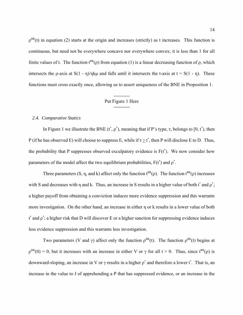
14

ρBR(t) in equation (2) starts at the origin and increases (strictly) as t increases. This function is

continuous, but need not be everywhere concave nor everywhere convex; it is less than 1 for all

finite values of t. The function tBR(ρ) from equation (1) is a linear decreasing function of ρ, which

intersects the ρ-axis at S(1 - η)/ηkμ and falls until it intersects the t-axis at t = S(1 - η). These

functions must cross exactly once, allowing us to assert uniqueness of the BNE in Proposition 1.

----------Put Figure 1 Here

----------

2.4. Comparative Statics

In Figure 1 we illustrate the BNE (t*, ρ*), meaning that if P’s type, τ, belongs to [0, t*), then

P (if he has observed E) will choose to suppress E, while if τ > t*, then P will disclose E to D. Thus,

the probability that P suppresses observed exculpatory evidence is F(t*). We now consider how

parameters of the model affect the two equilibrium probabilities, F(t*) and ρ*.

Three parameters (S, η, and k) affect only the function tBR(ρ). The function tBR(ρ) increases

with S and decreases with η and k. Thus, an increase in S results in a higher value of both t* and ρ*;

a higher payoff from obtaining a conviction induces more evidence suppression and this warrants

more investigation. On the other hand, an increase in either η or k results in a lower value of both

t* and ρ*; a higher risk that D will discover E or a higher sanction for suppressing evidence induces

less evidence suppression and this warrants less investigation.

Two parameters (V and γ) affect only the function ρBR(t). The function ρBR(t) begins at

ρBR(0) = 0, but it increases with an increase in either V or γ for all t > 0. Thus, since tBR(ρ) is

downward-sloping, an increase in V or γ results in a higher ρ* and therefore a lower t*. That is, an

increase in the value to J of apprehending a P that has suppressed evidence, or an increase in the

15

likelihood that P actually observed E (when he reported φ), increases J’s incentive to investigate,

and P’s anticipation of this results in greater deterrence of evidence suppression.

Finally, the parameter μ affects both functions; an increase in μ decreases tBR(ρ), whereas it

increases ρBR(t). This implies a definite effect of μ on t*: an increase in μ results in a decrease in

t*. That is, an increase in the effectiveness of an investigation ultimately reduces the threshold for

disclosure and, hence, the extent of evidence suppression. But we are not able to determine the

effect of an increase in μ on ρ*; the direct effect is to increase J’s incentive to investigate but this is

offset to a greater or lesser extent by the increased deterrence of suppression (since F(t*) falls).

The distributions F(τ) and H(c) can also be perturbed in the sense of first-order stochastic

dominance. F(τ) strictly first-order stochastically dominates ö(τ) if ö(τ) > F(τ) for all τ > 0. Here,

ö places more weight on lower values of τ than F does. This means that ö(τ) represents

stochastically lower disutility for convicting innocent defendants. For example, such a shift could

represent conditioning on D’s past criminal record; thus, P might experience stochastically lower

disutility from convicting a D who has engaged in previous bad behavior, but who is innocent of this

crime. Analogously, H(c) strictly first-order stochastic dominates ,(c) if ,(c) > H(c) for all c 0 (0,

4). This dominance represents stochastically lower disutility of investigation under , than under

H, since , places more weight on lower c-outcomes.

Only the curve ρBR(t) is affected by a change in these distributions. In both cases, this curve

still starts at ρBR(0) = 0, but it is everywhere higher under ö(@) or ,(@). Thus, a stochastically lower

disutility for convicting innocent defendants on the part of P encourages J to investigate more often

for any conjectured threshold: ρ* increases and t* decreases. It may seem counterintuitive that ρ*

increases when t* decreases. But recall that the distribution of τ is also changing, and it is putting

16

more weight on lower values of τ. Let (ρ*, t*) be the equilibrium under F and let (ρ*N, t*N) be the

equilibrium under ö. Then ρ* < ρ*N implies that F(t*) < ö(t*N), despite the fact that t*N < t*. That

is, there is more evidence suppression under ö (despite the lower threshold), which justifies a

higher probability of investigation. Similarly, a stochastically lower disutility of investigation

results in a higher likelihood of investigation ρ* and a lower threshold t*.

3. Analysis for the Two-Prosecutor Model

Here we extend the base model to consider two versions of how information is handled by

a team of prosecutors. For simplicity, we restrict attention to teams with two prosecutors; the

versions will differ according to how knowledge of exculpatory evidence is (exogenously)

distributed within the team. Throughout this section the definitions of strategies, best responses, and

Bayesian Nash Equilibrium are the obvious analogues of Definitions 1-3 in Section 2; conveniently,

comparative statics results for the two-prosecutor models are the same as in Section 2.

We first assume that any exculpatory evidence is received by only one prosecutor (we call

this the 21, or “disjoint,” information configuration); next we assume that all exculpatory evidence

is known by both prosecutors (we call this the 22, or “joint,” information configuration). Thus, we

view the disjoint configuration as capturing compartmentalization of knowledge about the

exculpatory evidence, whereas the joint configuration represents common knowledge of the

possession of exculpatory evidence by the entire team.

Regardless of the information configuration, we assume that each P makes a simultaneous

and non-cooperative decision regarding disclosure (or suppression) of any exculpatory evidence in

his possession. The individual-decision assumption is realistic because each prosecutor has an

individual affirmative duty to disclose material exculpatory evidence under Brady; this derives from

17

a line of cases which have developed Brady jurisprudence and is reinforced by the ABA Rules of

Professional Conduct which specify an independent ethical responsibility for an individual P to

disclose exculpatory evidence.17 If a P decides that he wants to disclose E to D, it is reasonable to

assume that he finds a way to accomplish this.18

Before proceeding to the analysis, we describe some aspects that will be common to the two

versions of a team, and also indicate what aspects will be maintained consistent with the one-

prosecutor model. In particular, we will assume that the parameters λ, γ, μ, η, and k continue to

apply as previously-defined. Specifically, the penalty for suppressing evidence, k, is imposed on

each team member that is found to have suppressed evidence; moreover, we assume that clear

evidence of personal misconduct is required to impose k on that prosecutor. We assume that

prosecutor i (i 0 {1, 2}) has a type τi; the types are independently and identically drawn from the

distribution F(τ) and, importantly, only a prosecutor who actively suppresses exculpatory evidence

suffers a disutility loss. We assume that each team member receives a payoff S2 when D is

convicted. We also modify the judge’s return to investigation (formerly V) to indicate whether 1

or 2 prosecutors are found to have suppressed evidence. Thus, let Vi denote J’s payoff when i 0 {1,

2} prosecutors are found to have suppressed evidence; we assume that V2 > V1. Further, we modify

the distribution of J’s disutility of investigation. Let H2(c) denote the distribution of c when a team

of prosecutors is investigated; H2(c) will apply to both versions of the two-prosecutor model (later

17 Formal Opinion 09-454: “Prosecutor’s Duty to Disclose Evidence and Information Favorable to theDefense,” 2009. This ethical obligation does not require the evidence to be “material” (see p. 2 of the Opinion).

18 If a P is not supposed to contact D directly, then he can disclose E to a senior teammate, or the DA, or thecourt if necessary. The ABA rules state that “... supervisors who directly oversee trial prosecutors must make reasonableefforts to ensure that those under their direct supervision meet their ethical obligations of disclosure, and are subject todiscipline for ordering, ratifying or knowingly failing to correct discovery violations.” [emphasis added]. In theThompson case, one of the prosecutors confessed (when dying) his Brady violation to a senior colleague, who urged himto report it to the DA. He did not, but neither did the colleague, who was later sanctioned for this failure to report.

18

we allow this distribution to differ between configurations 21 and 22). Finally, we assume that

members of the team do not reward or punish each other; we relax this assumption in Section 5.

3.1. Exculpatory Evidence is Received by a Single Team Member

In the first version of our two-person team of prosecutors, we assume that the exculpatory

evidence (if any) is received by only one of the prosecutors, and it is random as to which one

receives it; moreover, the fact that the configuration is disjoint is common knowledge to all

participants (including J). Thus, if prosecutor P1 receives exculpatory evidence, then he knows that

P2 did not receive it. On the other hand, if P1 does not receive exculpatory evidence, then he does

not know whether P2 received exculpatory evidence (since none may have been found, either

because it did not exist or it did exist but was not discovered). More formally, if D is innocent, then

Nature draws E with probability γ and randomly reveals it to one of the prosecutors.

The random-allocation assumption is reasonable, including with regard to what J is likely

to know should she later consider launching an investigation of the prosecutorial team. Even if

legitimate tasks of case preparation are divided between Ps, the receipt of exculpatory evidence can

occur within either prosecutor’s bundle of tasks. For instance, if forensic evidence is managed by

one team member while another deals with witnesses, then either task may uncover exculpatory

evidence. A witness for the prosecution may be uncertain, or his or her credibility may be subject

to impeachment. P may choose not to disclose these witness weaknesses, or may even coach the

witness in how to testify, both of which are Brady violations. On the other hand, if a piece of

physical evidence is brought to the attention of the P in charge of forensic evidence, he can choose

not to have it tested, or to have it tested but then to suppress the report should it be exculpatory. In

both cases, individual Ps can take such actions without the knowledge of a teammate. Further, either

19

P may receive information (e.g., via a phone call, or contact by a policeman or a witness) regarding

exculpatory evidence, independent of their assigned tasks. Finally, as the Thompson case shows,

such evidence can get “lost.”19

Consider P1's payoff function (a parallel analysis applies to P2). It now depends on: the

vector of types for P1 and P2, denoted (τ1, τ2); the vector of evidence states for P1 and P2, denoted

(θ1, θ2); and the vector of reports by P1 and P2, denoted (r1, r2). The general form of P1's payoff is:

πP1(r1, r2; θ1, θ2, τ1, τ2). As before, any prosecutor that has observed φ must also report φ. There are

several possible outcomes and associated payoffs, and these will be relevant in Section 4 when we

consider endogenous information configurations. However, our immediate interest is in

characterizing P1's behavior, and P1 only has a decision to make when θ1 = E. Moreover, in this

case, P2 has no decision to make (he must report φ, as that is what he observed). If P1 observes E,

the relevant payoff comparison for P1 is between πP1(E, φ; E, φ, τ1, τ2) and πP

1(φ, φ; E, φ, τ1, τ2). The

former equals zero since, once exculpatory evidence is disclosed, the case against D is dropped,

while the latter equals S2(1 - η) - τ1 - ηkμρ^, where ρ^ is now interpreted as P1's conjectured

probability that J investigates when both prosecutors reported φ and D later discovered and

submitted E. Notice that this comparison is the same as in the one-prosecutor discussion except that

S = S2, so P1 should disclose if τ1 > t21(ρ^), where t21(ρ

^) / max {0, S2(1 - η) - ηkμρ^}.

Now consider J’s payoff. Since there is no interaction between P1 and P2 (only one makes

a decision) and they are otherwise identical, the equilibrium threshold will be the same for both of

19 In the robbery case mentioned earlier, one of the prosecutors (Whittaker) received a lab report concerningblood evidence and claimed to have placed it on a colleague’s desk (Williams), but Williams denied having ever seenit. Thomas observes that: “The report was never disclosed to Thompson’s counsel.” See Connick v. Thompson, at 55. Moreover, it appears that the prosecution chose to remain ignorant of Thompson’s blood type, thereby avoiding knowingthat they had material evidence (since it differed from the blood evidence type).

20

them. Thus, J should have a common conjectured threshold for P1 and P2, which we denote as t^.

When D provides E, but both P1 and P2 reported φ, J constructs a posterior belief about whether one

of the prosecutors suppressed evidence (the alternative is that both Ps actually did observe φ). More

precisely, the report pair (φ, φ) occurs if: (1) no exculpatory evidence was found, which happens

with probability 1 - γ; or (2) if exculpatory evidence was found but suppressed, which happens with

probability γF(t^). This latter expression includes the probability that it was found (γ) and it is P1

who received the evidence (with probability ½) and he suppressed it because τ1 < t^, plus the

probability that it was found (γ) and it is P2 who received the evidence (with probability ½) and he

suppressed it because τ2 < t^. Thus, J’s posterior belief that evidence was suppressed is given by

γF(t^)/[1 - γ + γF(t^)]. This posterior belief is the same as in the one-prosecutor case.

Hence, J observes her disutility of investigation, which is still denoted as c but is now drawn

from the distribution H2(c), and decides whether to investigate (d = 1) or not (d = 0). J’s payoff from

investigation is now πJ(1; c) = V1μγF(t^)/[1 - γ + γF(t^)] - c and her payoff from not investigating is

πJ(0; c) = 0. The parameter V1 appears here because only one P can be suppressing evidence and

thus only one P can be punished. Similar to the analysis in Section 2, it is clear that πJ(1; c) =

V1μγF(t^)/[1 - γ + γF(t^)] - c > πJ(0; c) = 0 whenever c < V1μγF(t^)/[1 - γ + γF(t^)], so J investigates if

c is low enough and does not investigate otherwise. As before, it will be more intuitive to work with

the following functions which summarize best-response behavior by the Ps and J (respectively):

tB2

R1(ρ) / S2(1 - η) - ηkμρ; (5)

ρB2

R1(t) / H2(V1μγF(t)/[1 - γ + γF(t)]). (6)

A Bayesian Nash Equilibrium for this version of the two-prosecutor team, denoted (t*21, ρ*21),

is defined analogously to the one in Section 2: both prosecutors and the judge play mutual best

21

responses. The function ρB2

R1(t) starts at the origin and increases (strictly) as t increases. The function

tB2

R1(ρ) is a linear decreasing function of t, which starts at S2(1 - η)/ηkμ on the ρ-axis and falls linearly

until it reaches the horizontal axis at t = S2(1 - η). The functions tB2

R1(ρ) and ρB

2R1(t) cross exactly once

(so t*21 > 0), which establishes the following result.

Proposition 2. There is a unique BNE (t*21, ρ*21), where t*21 0 (0, S2(1 - η)) and ρ*

21 0 (0, 1),given by the pair of equations:

t*21 = S2(1 - η) - ηkμρ*21; (7)

ρ*21 = H2(V1μγF(t*21)/[1 - γ + γF(t*21)]). (8)

3.2. Exculpatory Evidence is Received by Both Team Members

We now consider configuration 22 wherein any exculpatory evidence is automatically

received by both members of the team. That is, if either P observes E (respectively, φ), then it is

common knowledge, within the team, that both know E (respectively, φ). J knows the configuration,

but not whether E was observed. Now both Ps have decisions to make; we assume that they make

their disclosure decisions simultaneously and noncooperatively, based only on their own private

information (i.e., their disutility of causing an innocent defendant to be convicted).20

Consider P1's payoff; again, the general form it takes is πP1(r1, r2; θ1, θ2, τ1, τ2). However, now

it must be that θ1 = θ2; either both team members observe E or both observe φ (and, in this latter

case, both must report φ). For convenience, we will focus on those events in which P1 has a

decision to make; we will fill out the details of the payoffs for the other events later when we

endogenize the information structure. If P1 observes E, then disclosing it will yield πP1(E, r2; E, E,

τ1, τ2) = 0 for all (r2, τ1, τ2); P2 will receive the same payoff. On the other hand, if P1 reports φ (i.e.,

20 If utility were transferable, the team could use an incentive-compatible mechanism to elicit information abouttheir τ-values and to recommend whether to disclose E to D. We briefly address this in footnote 22 and the Appendix.

22

P1 suppresses the exculpatory evidence), then if P2 discloses E, P1 will receive πP1(φ, E; E, E, τ1, τ2)

= 0 for all (τ1, τ2); whereas if P2 also reports φ, P1 will receive πP1(φ, φ; E, E, τ1, τ2) = S2(1 - η) - τ1 -

ηkμρ^, where ρ^ is again interpreted as P1's and P2's common conjectured probability that J

investigates when both prosecutors report φ and D provides E. Note that we assume P1 only suffers

the disutility τ1 if D is actually falsely convicted; if P1 suppresses evidence but his partner discloses

it, P1 does not suffer the disutility τ1 (as his action did not cause an innocent D to be convicted).

Since P1 and P2 act simultaneously and without knowledge of each others’ τ-values, P1 must

have a conjecture about P2's behavior (much as J must have a conjecture about both P1's and P2's

behavior). We assume that P1 and J maintain a common conjectured threshold, denoted t^, such that

all P2 types with τ2 < t^ are expected to report φ when they observe E. Then P1's expected payoff

when he observes E and reports φ is given by: 0@[1 - F(t^)] + [S2(1 - η) - τ1 - ηkμρ^]F(t^). Thus, P1

should disclose if τ1 > t22(ρ^), where t22(ρ

^) / max {0, S2(1 - η) - ηkμρ^}, which is independent of the

conjecture about P2's threshold. As is readily apparent, t22(ρ^) = t21(ρ

^). Similarly, P2's best response

(to his conjecture about the probability that J will investigate, ρ^) is independent of his conjecture

about P1, and is the same in a team with joint information and a team with disjoint information.

This again leads to the same threshold rule, now for each prosecutor.

Now consider J’s payoff. Since there is no interaction between P1 and P2 and they are

otherwise identical, the equilibrium threshold will be the same for both of them. Thus, J should have

a common conjectured threshold, which we denote as t^. When D provides E, but both prosecutors

reported φ, J must construct a posterior belief about whether they suppressed evidence. The report

pair (φ, φ) would have occurred if: (1) no exculpatory evidence was found, which happens with

probability 1 - γ; or (2) if exculpatory evidence was found but both prosecutors suppressed it, which

23

happened with probability γ(F(t^))2. Thus, J’s posterior belief that the prosecutors suppressed

evidence is γ(F(t^))2/[1 - γ + γ(F(t^))2]. This posterior belief is not the same as in the team with

disjoint information (the 21 configuration); in the team with joint information, each prosecutor can

serve a “whistle-blowing” role by disclosing E (thus preventing the conviction of an innocent D).

Assume that J’s disutility of investigation in the case of joint information is still drawn from

the distribution H2(c); that is, as discussed earlier, the disutility of investigation depends only on the

number of team members. We also assume that the investigation successfully verifies suppression

by both team members (with probability μ) or neither (with probability 1 - μ); it never verifies

suppression by only one team member when both have engaged in suppression. Finally, J’s payoff

from an investigation that verifies suppression of evidence by both prosecutors, denoted V2, is

assumed to be at least V1. J observes her disutility of investigation and decides whether to

investigate (d = 1) or not (d = 0). J’s payoff from investigation is πJ(1; c) = V2μγ(F(t^))2/[1 - γ +

γ(F(t^))2] - c and her payoff from not investigating is πJ(0; c) = 0. It is clear that πJ(1; c) =

V2μγ(F(t^))2/[1 - γ + γ(F(t^))2] - c > πJ(0; c) = 0 whenever c < V2μγ(F(t^))2/[1 - γ + γ(F(t^))2].

Best response behavior for the Ps and J are summarized by:

tB2

R2(ρ) / S2(1 - η) - ηkμρ; (9)

ρB2

R2(t) / H2(V2μγ(F(t))2/[1 - γ + γ(F(t))2]). (10)

Clearly, tB2

R2(ρ) = tB

2R1(ρ); however, ρB

2R2(t) and ρB

2R1(t) are not as easily-ordered. We first provide the

characterization of the BNE for the 22 configuration and then we compare the equilibrium amounts

of suppression and investigation.

A BNE for this version of the two-prosecutor team, denoted (t*22, ρ*22), is defined analogously

as in Section 2: both prosecutors and the judge play mutual best responses. As in the 21 case, it is

24

clear that t*22 > 0, and that the function ρB2

R2(t) starts at the origin and increases (strictly) as t increases.

The functions tB2

R2(ρ) and ρB

2R2(t) cross exactly once, establishing the following result.

Proposition 3. There is a unique BNE (t*22, ρ*22) where t*22 0 (0, S2(1 - η)) and ρ*

22 0 (0, 1),given by the pair of equations:

t*22 = S2(1 - η) - ηkμρ*22; (11)

ρ*22 = H2(V2μγ(F(t*22))

2/[1 - γ + γ(F(t*22))2]). (12)

Figure 2 depicts equilibrium in the 21 and 22 configurations, assuming that V2 = V1. Both

ρB2

R2(t) and ρB

2R1(t) functions start at the origin and increase with t. Both are based on the distribution

H2(c), but for any given t, their arguments are not the same. However, if V2 was equal to V1, then

since (F(t))2 < F(t) for t > 0, it follows that (F(t))2/[1 - γ + γ(F(t))2] < F(t)/[1 - γ + γF(t)]. Hence, we

conclude that ρB2

R2(t) < ρB

2R1(t) for all t > 0.21 This implies that t*22 > t*21 and ρ*

22 < ρ*21, as shown.

-----------Put Figure 2 here

-----------

Next consider the comparison between ρB2

R2(t) and ρB

2R1(t) as we increase V2 relative to V1.

When V2 = V1, these two functions cross at (t equals) infinity. As V2 is increased relative to V1,

this crossing point for ρB2

R2(t) and ρB

2R1(t) moves inwards towards the origin, eventually resulting in the

ρB2

R2(t) curve crossing P’s best response function where t*22 < t*21 and ρ*

22 > ρ*21. That is, as V2 becomes

sufficiently larger than V1, the ordering of the equilibria changes. We employ this result later.

Regardless of the ordering of the equilibrium thresholds for suppressing evidence and the

equilibrium likelihoods of investigation, we can order the equilibrium likelihoods of evidence

suppression in the two team environments. The equilibrium likelihood of evidence suppression

21 One could also contemplate a mixture of the 21 and 22 configurations, wherein neither the Ps nor J knowwhether the configuration is 21 or 22 when they choose their strategies. This results in the same best response functionfor the prosecutors, but J’s best response function lies between ρB

2R1 (t) and ρB

2R2 (t). This yields qualitatively similar results.

25

under joint information is (F(t*22))2, since both prosecutors’ τ-values must fall below t*22 in order for

the evidence to be suppressed. The equilibrium likelihood of evidence suppression under disjoint

information is F(t*21), since only the τ-value of the recipient of the exculpatory evidence must fall

below t*21 in order for evidence to be suppressed. The following is proved in the Appendix.

Proposition 4. There is less evidence suppression in equilibrium under joint informationas compared to disjoint information. That is, (F(t*22))

2 < F(t*21).

Thus, even though the joint information configuration may result in a higher threshold for evidence

disclosure, the full effect will always be to reduce the likelihood of evidence suppression.22

Finally, one might think that the distribution of J’s disutility of investigating could depend

on whether the configuration is 21 or 22. For instance, in the 22 case, once one P’s suppression has

been verified, this P can give evidence against the other P, potentially lowering J’s disutility of

investigation by reducing resource costs. If J’s expected disutility of investigation is stochastically

lower in the 22 (as compared to the 21) configuration, this has a similar effect as increasing V2

relative to V1. That is, the function ρB2

R2(t) increases for every value of t > 0, resulting in a decrease

in t*22, which reinforces the result in Proposition 4.

3.3. Prosecutor Preferences over Exogenously-Determined Configurations

In this subsection, we provide the equilibrium payoff functions under the two exogenous

information configurations, and determine sufficient conditions for a P to prefer the disjoint

information configuration to the joint information configuration. Let Π*21 denote P1's ex ante

expected payoff in a two-prosecutor team with configuration 21. Then:

22 This likelihood of suppression will increase if utility is transferable and a Groves-Clarke mechanism (seeMas-Colell, Whinston, and Green (1995), pp. 878-879) is used to coordinate the Ps’ choices to suppress evidence. Seethe Appendix for the details on this and why, since it involves supporting and enhancing prohibited behavior, and sucha mechanism requires ex ante commitment by both prosecutors, we do not pursue this angle further.

26

Π*21 = (1 - λ)S2 + λ(1 - γ)S2(1 - η) + (λγ/2)S2(1 - η)F(t*21)

+ (λγ/2)I{S2(1 - η) - ηkμρ*21 - τ}dF(τ), (13)

where the integral is over [0, t*21]. This expression is interpreted as follows. The first term reflects

the fact that with probability 1 - λ, D is actually guilty, so there is no exculpatory evidence and D

will therefore be convicted, yielding a payoff of S2. The second term reflects the fact that with

probability λ, D is innocent but, with probability (1 - γ), neither P observes E; thus D is convicted,

yielding a payoff of S2, which is lost if D subsequently observes E and the conviction is vacated,

which occurs with probability η. Note that P1 loses the value of the conviction, but does not suffer

an internal disutility because his actions did not cause the false conviction. The third term reflects

the fact that, with probability λ, D is innocent and with probability γ/2, P2 observes exculpatory

evidence, which he suppresses if τ2 < t*21 (i.e., with probability F(t*21)). In this event, D is convicted,

but the conviction is lost if D subsequently provides E, which happens with probability η. Since

equation (13) is P1's expected payoff and the third term assumes that P2 suppressed, P1 does not

incur τ1 or k. Finally, the last term reflects the fact that, with probability λγ/2, D is innocent and P1

observes E. If P1’s type τ1 is less than t*21, then he suppresses the exculpatory evidence, which yields

the payoff S2(1 - η) - ηkμρ*21 - τ1; this type-specific payoff is integrated over those types that suppress

the evidence. The same equation provides P2's ex ante expected payoff in the 21 configuration.

Next, consider the 22 configuration. Let Π*22 denote P1's ex ante expected payoff in a two-

prosecutor team with joint information. Then:

Π*22 = (1 - λ)S2 + λ(1 - γ)S2(1 - η) + λγF(t*22)I{S2(1 - η) - ηkμρ*

22 - τ}dF(τ), (14)

where the integral is over [0, t*22]. The first two terms are the same as in the 21 model. The third

term reflects the fact that, with probability λγ, D is innocent and both P1 and P2 observe exculpatory

27

evidence, which P2 suppresses if τ2 < t*22 (i.e., with probability F(t*22)). If P1’s type τ1 is less than t*22,

then he also suppresses the exculpatory evidence, which yields the payoff S2(1 - η) - ηkμρ*22 - τ1; this

type-specific payoff is integrated over those P1 types that suppress the evidence.

Comparing the 21 and 22 cases, we obtain the following (see the Appendix for the proof).

Proposition 5. If t*22 < t*21 (or t*22 > t*21, but the difference is sufficiently small), then ex ante,a prosecutor would prefer to work in a team with disjoint information than in a team withjoint information.

Thus, for example, if V2 is sufficiently larger than V1, then the Ps prefer there to be only one

informed prosecutor (i.e., the 21 configuration), as the prospect of receiving V1 reduces J’s

incentive to investigate (as compared to her receiving V2). A second intuition for this preference

is that there are circumstances under which P1 would prefer to suppress the exculpatory information

(e.g., low τ1), but his teammate is likely to disclose it if he also observes it (e.g., low t*22). The

disjoint information configuration allows P1 to control the disclosure decision when he alone

observes E. Finally, if P2 controls the disclosure decision, then P1 benefits when P2 suppresses.

4. Endogenous Determination of the Information Configuration

In subsection 3.1 we assume that only one team member received any exculpatory evidence

(randomly, either P1 or P2). In subsection 3.2 we assume that any exculpatory evidence was

commonly known by both team members. In both analyses, J knows whether the configuration is

21 or 22. In this section, we examine which configuration(s) can emerge as part of an overall BNE

for the game with endogenous information configuration, assuming that J cannot observe the chosen

configuration. Thus, J’s decision regarding investigation will depend on her conjecture about the

information configuration within the prosecutorial team.

We consider two ways of endogenizing the information configuration. One way involves

28

the team members coordinating ex ante and committing as to whether the information configuration

will be joint or disjoint. The other way of endogenizing the information configuration involves a

single team member randomly receiving any E and then deciding whether to share it with his

teammate. That is, starting in the 21 configuration, will a P who receives exculpatory evidence

convert the configuration into 22 by sharing with the other P? In this analysis the decision is made

at the interim stage (after the types and any exculpatory evidence have been realized).

4.1. Ex ante Choice of Information Configuration

When J cannot observe the two-prosecutor information configuration, we have to incorporate

conjectures on J’s part. We then ask whether there can be an equilibrium to the overall game

wherein the team of prosecutors, ex ante, chooses a joint information configuration. If J expects the

team to choose a joint information configuration, then J will investigate with probability ρ*22. If P1

and P2 choose a joint information configuration, each can expect a payoff of Π*22 as given in

equation (14). What if, unobserved by J, P1 and P2 deviate to a disjoint configuration (and play in

a subgame-perfect way thereafter)? Having deviated to a disjoint information configuration, they

might consider changing their equilibrium thresholds but, in fact, t*22 is still a best response to ρ*22.

In the Appendix we show that this deviation is always preferred, so there cannot be an equilibrium

wherein the team chooses a joint information configuration.

Next we ask whether there can be an equilibrium wherein the team chooses the disjoint

configuration. If J expects the team to choose a disjoint configuration, then J will investigate with

probability ρ*21. If P1 and P2 choose a disjoint configuration, each can expect a payoff of Π*

21 as

given in equation (13). What if, unobserved by J, P1 and P2 deviate to a joint configuration (and

play in a subgame-perfect way thereafter)? Although they might consider changing their

29

equilibrium thresholds, t*21 is still a best response to ρ*21. As shown in the Appendix, this deviation

is never preferred and hence there is an equilibrium wherein the team chooses the disjoint

configuration. Thus, when P1 and P2 choose the information configuration ex ante, but J cannot

observe their choice, then the only equilibrium involves a disjoint configuration.

4.2. Interim Choice of Information Configuration

In this case, we think of the information configuration as involving exculpatory evidence

being observed by either P1 or P2 (with equal probability), but then the observing prosecutor can

choose to share the information with his teammate or to suppress it (both from the teammate and the

defendant). At the interim stage, both prosecutors know their own types.

Suppose that P1 observes exculpatory evidence. Can there be an equilibrium wherein P1

first shares this evidence with P2, and then each continues optimally (i.e., each decides

simultaneously and noncooperatively whether to disclose E to D)? Suppose that J expects

exculpatory evidence to be shared, and therefore investigates with probability ρ*22. If a P1 of type

τ1 shares the evidence with P2 (who does not disclose to D with probability F(t*22)), then P1 can

expect a payoff of F(t*22)(S2(1 - η) - ηkμρ*22 - τ1) if he does not disclose E to D. Thus, the threshold

for P1 to disclose remains t*22. However, by deviating to not sharing the evidence with P2, P1 will

obtain a payoff of S2(1 - η) - ηkμρ*22 - τ1 if he does not disclose E to D. Thus, when P1 has observed

E and when τ1 < t*22, then P1 will defect from the putative equilibrium involving evidence sharing,

so as to preempt any possibility of his teammate disclosing E to D.

Alternatively, can there be an equilibrium wherein P1 does not share exculpatory evidence

with P2? Suppose that J expects exculpatory evidence not to be shared, and therefore investigates

with probability ρ*21. Then if a P1 of type τ1 does not share the evidence with P2, then P1 can expect

30

a payoff of S2(1 - η) - ηkμρ*21 - τ1 if he does not disclose E to D, so he will disclose if τ1 > t*21.

However, by deviating to sharing the evidence with P2, P1 will obtain a lower payoff of F(t*21)(S2(1 -

η) - ηkμρ*21 - τ1) if he does not disclose E to D. Thus (following the deviation) the threshold for P1

to disclose to D remains t*21, but P1 will never deviate to sharing exculpatory evidence with P2

because this would only give P2 the opportunity to disclose E when P1 prefers to suppress it.

When the decision regarding whether to share exculpatory evidence with a teammate is taken

at the interim stage, the only equilibrium involves P1 not sharing with P2 when P1 prefers to keep

the evidence from D; when P1 prefers to disclose to D, he can do it directly without previously

sharing it with his teammate.

The results of subsections 4.1 and 4.2 are summarized in the following proposition.

Proposition 6. Assume that J does not observe the information configuration within theteam. If P1 and P2 choose the information configuration either jointly at the ex ante stage,or by making an individual decision about information sharing at the interim stage, then theoverall equilibrium involves a disjoint information configuration.

5. The Effect of Angst, Office Culture, and Costly Suppression Effort

In this section we consider three extensions of the model examined in Section 3 and 4. We

first consider the effect of accounting for “angst” on the part of an uninformed P concerning

potential bad behavior by a teammate. We next consider “office culture” wherein colleagues and/or

supervisors may reward or punish individual Ps for behavior of which they approve or disapprove.

Finally, we consider the choice by Ps of costly effort to reduce the likelihood (η) that D will find

exculpatory evidence that has been suppressed.

5.1. Angst

Recall that, in a 21 configuration, P1 benefits from a false conviction that P2 causes; even

if D finds exculpatory evidence and the conviction is overturned, P1 does not suffer the disutility

31

of having caused the false conviction (since P2 caused it and P1 was unaware). What if, however,

P1 suffered angst about the possibility that P2 might suppress E? Angst might arise for P1 from

either: 1) the expectation of repugnance for a possible suppression action by P2; or 2) from

anticipation of the potential embarrassment P1 might suffer upon revelation of a teammate’s bad

behavior. Let angst be modeled as a disutility for P1 of ατ1, where α > 0, whenever P2's evidence

suppression caused a false conviction of which P1 was (at the time) unaware. Then the term S2(1 -

η) in the third term in equation (13) would become S2(1 - η) - αXE(τ1)F(t*21), where X = 1 in the

repugnance case above while X = ημρ*21 for the embarrassment case. Our maintained assumption

is that α = 0, but the results in Section 4.1 would continue to hold if α is sufficiently small, which

we believe is most plausible (especially with respect to the embarrassment version, due to the

multiple fractions entering the term). The results in Section 4.2 continue to hold for any size of α.

5.2. Office Culture

In this subsection we consider an extension in the case of a team with a 21configuration

(since that is the predicted equilibrium configuration; see Section 4). We have assumed that each

P’s type is his own private information, and that each P makes his disclosure decision

noncooperatively. Moreover, we have ruled out transferable utility, so neither P can offer or extract

a payment from the other. However, it is very possible that informal incentives operate within the

office. Office culture could reward or punish disclosure, so that P1's payoff from disclosing is now

πP1(E, φ; E, φ, τ1, τ2) = β. If β > 0, then disclosure is rewarded, whereas if β < 0, then it is punished.

For example, colleagues can be more or less cooperative and supervisors can provide better or worse

future assignments. This has the predictable effect of reducing suppression and investigation if

disclosure is rewarded, and increasing suppression and investigation if disclosure is punished.

32

A more subtle version of informal sanctions could be imposed by a teammate. For instance,

suppose that P1 received exculpatory evidence and disclosed it; P2 can evaluate what his decision

would have been had he (rather than P1) received the evidence. If P2 would have chosen to disclose

it as well, we assume that P2 does not impose any informal sanctions on P1. But if P2 would have

suppressed it, then P2 could impose an informal sanction in the amount σ > 0 on P1. This informal

sanction may consist of disrespect, uncooperativeness, or sabotage in future interactions with P1.

The fact that it is informal tends to limit the magnitude of σ, as overall office culture may discourage

informal sanctions, or at least prefer the response be limited so as not to attract public scrutiny.

Revisiting the analysis of subsection 3.1, P1's payoff from suppressing E remains S2(1 - η) -

τ1 - ηkμρ^, where ρ^ is P1's conjectured probability that J investigates when both prosecutors report

φ and D later provides E. But P1's expected payoff when he discloses is now πP1(E, φ; E, φ, τ1, τ2)

= -σF(t^), since P1 conjectures that all P2 types with τ2 < t^ would have reported φ if they had been

the one that observed E. Now P1's best response is to both conjectures, t^ and ρ^: P1 should disclose

if τ1 > t21(t^, ρ^), where t21(t^, ρ^) / max {0, S2(1 - η) - ηkμρ^ + σF(t^)}. P2 should follow the analogous

rule if he is the one that observes E. Notice that if P1 conjectures that P2 would have used a higher

threshold t^, then P1's best response is also to use a higher threshold.

We characterize an equilibrium in which P1 and P2 use the same threshold. J uses a common

conjecture t^ for both P1 and P2, so her problem is unchanged from that modeled in Section 3.1. This

results in the same best-response likelihood of investigation, ρB2

R1(t^) = H2(V1μγF(t^)/[1 - γ + γF(t^)]).

Let the equilibrium threshold for P1 and P2 be denoted t*21(σ). J’s equilibrium likelihood of

investigation, now also a function of σ, will be denoted ρ*21(σ). As before, it is clear that t*21(σ) = 0

cannot be part of an equilibrium; some evidence suppression will be necessary to motivate

33

investigation by J. Thus, a Bayesian Nash Equilibrium (t*21(σ), ρ*21(σ)) is a solution to the equations:

t = S2(1 - η) - ηkμρ + σF(t); (15)

ρ = H2(V1μγF(t)/[1 - γ + γF(t)]). (16)

Note that equation (15) defines t*21(σ) implicitly. It will be easier to visualize and understand

the BNE if we solve equation (15) for ρ in terms of t, which we will denote as b21(t; σ). The function

ρ = b21(t; σ) / [S2(1 - η) - t + σF(t)]/ηkμ is increasing in σ for all t > 0, but begins at the same vertical

intercept, S2(1 - η)/ηkμ, for all σ (and it lies above b21(t; 0) for all t > 0). When σ = 0, this is simply

the usual negatively-sloped line that crosses the horizontal axis at S2(1 - η). For σ > 0, we can no

longer be sure that b21(t; σ) is downward-sloping everywhere; however, it will cross the horizontal

axis when t gets sufficiently large. It is clear that there is at least one BNE, (t*21(σ), ρ*

21(σ)), and that

t*21(σ) > t*

21(0) and ρ*21(σ) > ρ*

21(0). That is, informal sanctions result in more suppression and more

investigation. Since b21(t; σ) need not be everywhere downward-sloping, it is possible that multiple

BNE exist; however, all BNE for σ > 0 involve more evidence suppression and more investigation

than the BNE for σ = 0. The functions b21(t; σ), b21(t; 0), and ρB2

R1(t) are graphed in Figure 3 below;

a scenario with three BNEs is depicted. Note that since ρB2

R1(t) is increasing in t, all the equilibria are

ordered, with higher t-thresholds associated with higher likelihoods of investigation.

Proposition 7. There is at least one BNE (t*21(σ), ρ*21(σ)) given by equations (15)-(16). For

any BNE with σ > 0, t*21(σ) > t*21(0) and ρ*21(σ) > ρ*

21(0).

-----------Put Figure 3 here

-----------

Finally, within the 22 configuration another type of informal sanction is possible.23 If P1

discloses but P2 suppresses, then there is no risk of formal sanctions for P2 (because no conviction

23 We thank Giri Parameswaran for pointing out this scenario and the resulting full-disclosure equilibrium.

34

occurs), but P1 could impose an informal sanction on P2. This can also result in multiple

equilibrium thresholds for the prosecutors; one type of equilibrium is similar to those described

above but another equilibrium involves no suppression by either prosecutor. In particular, if P2

conjectures that P1 will always disclose (regardless of type), then it is a best response for P2 to

always disclose as well (and J need not investigate). But then neither P can ever benefit from

suppressing evidence. If the prosecutors can coordinate on a particular equilibrium, then they will

avoid this one; moreover, if this is the anticipated equilibrium in the 22 configuration, then they will

have even more reason to avoid choosing the 22 configuration.

5.3. Costly Suppression Effort

Assume that a P who has observed E and wishes to suppress it can influence the likelihood

that D will subsequently discover E by engaging in suppression effort e at a cost of e2/2, yielding

a likelihood η(e) that D later discovers E, where ηN(e) < 0 and ηO(e) > 0. We assume that this effort

is expended only after P has decided to suppress E.24 Resource costs of active suppression adds

some minor complications, but again it does not affect the results in any material way.

In the 21configuration, a P of type τ that considers suppression expects to gain S2(1 - η(e)) -

η(e)kμρ^ - τ - e2/2 and will choose e to maximize this expression (which is strictly concave in e, with

a unique interior solution). This yields an optimal suppression effort e*(ρ^) that is increasing in ρ^,

and independent of τ. The best-response disclosure threshold for P is now tBR(ρ) = S2(1 - η(e*(ρ)) -

η(e*(ρ))kμρ - (e*(ρ))2/2 for any given ρ. Although no longer linear in ρ, tBR(ρ) is still a downward-

sloping function in (t, ρ) space; by the envelope theorem, tBRN(ρ) = - η(e*(ρ))kμ. It crosses the

24 If P has not observed E then let η0 be the likelihood that D discovers E; this would replace η in the secondterm of equations (13) and (14), which cannot affect any of the analysis. Notice that there is no reason to assume, forexample, that η0 = η(0). For example, Thompson’s defense would not have found the blood evidence in the burglarycase if the prosecution had not already discovered it.

35

horizontal axis at t = S2(1 - η(e*(0)) - (e*(0))2/2. J’s best response function for the 21 configuration

is independent of η, and is unaffected by P’s effort suppression choice. The best response functions

continue to have a unique intersection point that provides the BNE. The profit function Π*21 must

be modified to reflect the effort suppression cost (e*(ρ*21))

2/2, which now appears in the integrand.

In addition, the endogenous value of η(e*(ρ*21)) appears in the third and fourth terms of Π*

21.

In modeling suppression effort in the 22 configuration, there are many possible ways to think

about this. For instance, when is effort expended? Whose effort matters? One plausible model

assumes that this effort is (again) expended only after the outcome of the disclosure decisions is

realized. That is, first P1 and P2 decide whether or not to disclose; if both choose not to disclose,

then they each choose suppression effort simultaneously and non-cooperatively. Since they both

observed E, we assume that they both must take effort to suppress it (e.g., they must both hide or

destroy their copies of the lab report, they must both purge their emails, etc.), with a plausible

formulation being η(e1, e2) = η(min{e1, e2}). That is, the suppression chain is only as strong as its

weakest link. If both P1 and P2 have announced an intention not to disclose, then P1 will

subsequently choose effort e1 to maximize S2(1 - η(e1)) - η(e1)kμρ^ -τ1 - (e1)2/2, subject to e1 < e2, as

there is no return to going beyond e2, given the assumed functional form for η(e1, e2). For a given

value of ρ, there is a continuum of equilibria wherein e1 = e2, ranging from 0 to e*(ρ^) as defined

above. Among these, both Ps prefer the equilibrium wherein e1 = e2 = e*(ρ^), so we select that one;

this is also the common effort level they would choose if they cooperated on the choice of effort.

Now consider P1's choice between suppressing and disclosing E. If P1 discloses, then he

will receive a payoff of 0 whereas if he suppresses, then he anticipates a payoff of [S2(1 - η(e*(ρ^)) -

η(e*(ρ^))kμρ - (e*(ρ^))2/2 - τ1]F(t), where F(t) represents P1's conjectured probability that P2 will also

36

choose to suppress (in which case they each exert effort e*(ρ^)). Thus, P1's best-response disclosure

threshold is the same as in the 21 configuration above: tBR(ρ) = S2(1 - η(e*(ρ)) - η(e*(ρ))kμρ -

(e*(ρ))2/2 for any given ρ. J’s best response function for the 22 configuration is independent of η,

and is thus unaffected by the effort suppression choice. The best response functions continue to

have a unique intersection point that provides the BNE. The profit function Π*22 in equation (14)

must be modified to reflect the effort suppression cost (e*(ρ*22))

2/2, which now appears in the

integrand. The 21 configuration remains the unique equilibrium, as before.

6. Summary and Discussion

6.1 Summary

In this paper we model a prosecutor’s objective as a mixture of career concerns and moral

concerns about causing innocent defendants to be convicted. Furthermore, we extend the model

to a team of two prosecutors, each of whom has private information as to their individual disutility

for convicting the innocent, and both of whom would benefit from a win at trial. If exculpatory

evidence comes into the possession of the prosecution, it may choose to disclose or suppress it,

where suppression leads to an unwarranted conviction of the defendant. Suppression of exculpatory

evidence that is material to the defense is a violation of the defendant’s constitutional rights under

Brady v. Maryland, but can readily contribute to the prosecutor’s career success. We focus on

perfect exculpatory evidence so as to clarify the primary incentives for disclosure.

If exculpatory evidence is later discovered by the defense, the conviction is voided and a

judge may order an investigation, depending upon the value of pursuing possible prosecutorial

misconduct versus the judge’s disutility for this pursuit. We characterize the Bayesian Nash

Equilibrium in the game between the prosecution and the judge. In the team case we consider two

37

information configurations, one wherein only one of the two prosecutors received exculpatory

evidence (the disjoint configuration) and one wherein both received it (the joint configuration).

When the configuration is endogenous, the disjoint configuration is the unique equilibrium.

6.2 Discussion of Policy Implications

At present the prosecution is only required to turn over exculpatory evidence that is material,

which allows for discretionary choices on the part of a prosecutor that can result in a decision that

disclosure (either to D or to a prosecutorial teammate) is not required. Kozinski (2013, footnote 118,

p. xxiv) observes: “Lack of materiality is the Justice Department’s standard defense when it is

caught committing a Brady violation.” This is undoubtedly no less true at the state level. One direct

policy change could be to reduce the strategic opportunities for prosecutors to suppress evidence by

eliminating the materiality requirement. If this strategic discretionary decision could be avoided or

minimized, then evidence would be more broadly-shared within the prosecution team and with the

defense. There have been a number of calls for “open files,” so that evidence developed by the

prosecution that is relevant to the defense is promptly made available to both sides.25

The effect of such a change is captured in our analysis. Recall that in the model, the

parameter μ was the probability that an investigation ordered by J verifies P’s failure to disclose

material exculpatory evidence in his possession. In Section 2.4 we indicated that an increase in μ

led to an decrease in the set of types who are willing to suppress, measured by F(t*). Allowing P to

use materiality strategically as a defense for evidence suppression (e.g., as noted above by Kozinski)

means that the resulting value of μ is lower than it would otherwise be, leading to an increase in t*,

25 See the discussion and references in New York State Bar Association: Report of the Task Force on CriminalDiscovery, 2015. The report cites examples of broadened discovery procedures and statutes in major cities in the U.S.,as well as in states such as New Jersey, North Carolina, Ohio, and Texas.

38

and therefore in F(t*). That is, an investigation that found that some exculpatory evidence was not

included in the (otherwise) open files could provide a very clear signal of an intent to violate Brady.

A second policy change concerns the penalties for individual prosecutors. Since the U.S.

Supreme Court’s decision in Imbler v. Pachtman in 1976, prosecutors have enjoyed absolute

immunity from civil liability for activities “intimately associated with the judicial phase of the

criminal process.” (Imbler at 430). Prosecutors are (in principle) subject to criminal prosecution but,

Kozinski (2015, p. xxxix) observes that: “Despite numerous cases where prosecutors have

committed willful misconduct, costing innocent defendants decades of their lives, I am aware of only

two who have been criminally prosecuted for it; they spent a total of six days behind bars.”

California recently passed a law making it a felony for prosecutors to knowingly withhold or falsify

evidence; the sentence can run from 16 months to three years. Notice that improving μ, as discussed

above, means that the penalty k (in terms of fines or jail time) in our model is likely to be

considerably more salient, possibly encouraging more judges to pursue suspected Brady violations.

There is a range of penalties available to policy makers, some “softer” than direct liability.

Kozinski (2015, p. xxvi) suggests a “naming and shaming” strategy: “Judges who see bad behavior

by those appearing before them, especially prosecutors who wield great power and have greater

ethical responsibilities, must hold such misconduct up to the light of public scrutiny.” One might

expect that developing more common knowledge among trial judges that some of the prosecutors

they engage with have developed reputations for violating Brady may lead those judges to more-

readily refer cases for investigation.

A third policy change concerns providing incentives for prosecutorial offices to adhere to

both the spirit and letter of Brady. We found that: 1) office culture can be a positive force for

39

disclosure of exculpatory evidence, or a negative force; and 2) informal sanctions by individual team

members who would have chosen to suppress evidence (if they had discovered it) yields multiple

equilibria, but all of those equilibria lead to yet more suppression of evidence than occurs without

such informal sanctions.

While individual prosecutors enjoy absolute immunity from civil suit, municipalities can

be subject to liability if plaintiffs can demonstrate deliberate indifference via a pattern of similar

constitutional violations (see the majority opinion in Connick v. Thompson by Justice Thomas at 52).

This necessitates a scheme for accumulating information on Brady violations. To our knowledge,

while all states have judicial conduct commissions (so that complaints about the behavior of judges

can be filed, documented, and investigated) no such bodies exist for receiving, documenting, and

investigating complaints about prosecutorial conduct. As indicated earlier, some states handle

complaints via courts while others use the state bar. Establishing prosecutorial conduct commissions

in each state, with the power to document and investigate misconduct,26 means that public databases

of misconduct could be developed. This would allow patterns of behavior to be deduced, and

lawsuits against municipalities to be supported by patterns of behavior. Furthermore, it would also

allow documentation of egregious behavior to be used by those who desire to run for District

Attorney positions in political campaigns, drawing the electorate into more-informed decision-

making regarding what sort of prosecutorial office they want to have. Monetary leverage on

municipalities, and political pressure on chief prosecutors, to better monitor professional staff (and

modify office culture) could thus be a way to break down pernicious office culture that encourages

or tolerates Brady violations.

26 This would also reduce J’s costs and disutility associated with addressing suspected misconduct, therebyincreasing the deterrence effect of penalties for violating Brady.

40

Appendix

Proof of Proposition 4. To see that (F(t*22))

2 < F(t*21), we first make this argument assuming that V2

= V1. We then argue that an increase in V2 (holding V1 constant) reinforces the result. Recall thatρB

2R2(t) = H2(V2μγ(F(t))2/[1 - γ + γ(F(t))2]) and ρB

2R1(t) = H2(V1μγF(t)/[1 - γ + γF(t)]). If V2 = V1, then

ρB2

R2(t) < ρB

2R1(t) for all t > 0 because the expression X/[1 - γ + γX] is increasing in X and (F(t))2 < F(t).

Since the function tB2

R2(ρ) = S2(1 - η) - t - ηkμρ = tB

2R1(ρ) is downward-sloping and the functions ρB

2R2(t)

and ρB2

R1(t) are upward-sloping, the equilibrium likelihoods of investigation can be ordered: ρ*

22 < ρ*21.

Since ρ*22 = H2(V1μγ(F(t*

22))2/[1 - γ + γ(F(t*

22))2]) < ρ*

21 = H2(V1μγF(t*21)/[1 - γ + γF(t*

21)]) and H2 isincreasing in its argument, it follows that V1μγ(F(t*

22))2/[1 - γ + γ(F(t*

22))2] < V1μγF(t*

21)/[1 - γ +γF(t*

21)]. This inequality holds if and only if (F(t*22))

2 < F(t*21). Thus we have established the claim

under the assumption that V2 = V1. Now consider the effect of increasing V2. The expression F(t*21)

is unaffected because t*21 is based on V1. But an increase in V2 increases the function ρB

2R2(t) for every

t > 0, which results in an increase in ρ*22 and a decrease in t*

22. A decrease in t*22 reduces the

expression (F(t*22))

2, which reinforces the result that (F(t*22))

2 < F(t*21).

Proof of Proposition 5. Proposition 5 claims that Π*

21 > Π*22, at least for t*22 < t*21 or for t*22 > t*21, but

sufficiently close. In the 21 configuration, t*21 = S2(1 - η) - ηkμρ*21. Thus, Π*

21 can be re-written as:

Π*21 = (1 - λ)S2 + λ(1 - γ)S2(1 - η) + (λγ/2)S2(1 - η)F(t*21) + (λγ/2)I{t*21 - τ}dF(τ),

where the integral is over [0, t*21]. In the 22 configuration, t*22 = S2(1 - η) - ηkμρ*22. Thus, Π*

22 can bere-written as:

Π*22 = (1 - λ)S2 + λ(1 - γ)S2(1 - η) + λγF(t*22)I{t*22 - τ}dF(τ),

where the integral is over [0, t*22]. Recall that there is no clear ordering between t*22 and t*21. If V2

= V1, then t*22 > t*21, but a sufficient increase in V2 relative to V1 could, in principle, reverse thisinequality. Suppose that t*22 < t*21; then we claim that Π*

22 < Π*21. This follows from three facts. First

(where all integrals are over [0, t*21]):

S2(1 - η)F(t*21) > I{S2(1 - η) - ηkμρ*21 - τ}dF(τ) = I{t*21 - τ}dF(τ).

Second, I{t*21 - τ}dF(τ) (where the integral is over [0, t*21]) > I{t*22 - τ}dF(τ) (where the integral isover [0, t*22]). This latter result follows since the expression I0

x{x - τ}dF(τ) is increasing in x and t*21

> t*22 (the two terms are equal if t*21 = t*22). Third, the expression I{t*22 - τ}dF(τ) (where the integralis over [0, t*22]) is pre-multiplied by F(t*22) < 1. Combining these inequalities implies that Π*

21 > Π*22.

Since this inequality is strict, it will also hold for t*22 > t*21 (but sufficiently close).

Evidence Suppression in the 22 Configuration with Transferable UtilityIf Ps had transferable utility, then a team in a 22 configuration could use a direct mechanism

that: (1) would induce them to report their τ-values truthfully (to the mechanism); and (2) wouldrecommend the efficient decision (i.e., the one that maximizes the sum of their payoffs). To seehow, let wi / S2(1 - η) - τ i - ηkμρ^ denote Pi’s value for suppressing evidence; this may be positive

41

or negative. Let Wi denote Pi’s reported value of wi. If Wi + Wj < 0, then the mechanismrecommends that the evidence be disclosed; moreover, if Wj > 0, then Pi pays a “tax” of Wj to a thirdparty (so as not to affect Pj’s reporting). But if Wi + Wj > 0, then it recommends that the evidencebe suppressed; moreover, if Wj < 0, then Pi pays a “tax” of -Wj since Pi is changing the decision.

The taxes correspond to what would just compensate the other P for imposing an outcomehe does not prefer; however, the taxes are not paid to the other P, but rather to a third party (so asnot to affect the other P’s reporting strategy). This mechanism induces truthful revelation of τ-values and results in the efficient (for the team) recommendation: suppress evidence when theaverage disutility (τ1 + τ2)/2 < S2(1 - η) - ηkμρ^, and otherwise disclose it to D. That is, the disclosurethreshold is t22(ρ

^) / max {0, S2(1 - η) - ηkμρ^}, which is the same as without transferable utility.

Next we consider J’s payoff, assuming she knows the team employs a Groves-Clarkemechanism. J conjectures that a team observing E will suppress it whenever the average disutility(τ1 + τ2)/2 is less than some threshold t^. Thus, when D provides E, but the team reported φ, J’sposterior belief that the prosecutors are suppressing evidence is γFavg(t^)/[1 - γ + γFavg(t^)], whereFavg(t^) = Pr{(τ1 + τ2)/2 < t^}. J’s expected payoff from investigation is now V2μγFavg(t^)/[1 - γ +γFavg(t^)] - c. Thus J’s best response is to investigate whenever c < V2μγFavg(t^)/[1 - γ + γFavg(t^)].

The following functions summarize the best-response behavior (the superscript “BR”denoting best response has been replaced with “TU” denoting transferable utility):

tT2

U2(ρ) / S2(1 - η) - ηkμρ; and ρT

2U2(t) / H2(V2μγFavg(t)/[1 - γ + γFavg(t)).

Clearly, tT2

U2(ρ) = tB

2R2(ρ); the threshold value of t in terms of ρ remains the same, but now it

is the average disutility (τ1 + τ2)/2 that must meet that threshold in order to induce disclosure. However, ρT

2U2(t) = H2(V2μγFavg(t)/[1 - γ + γFavg(t)]) > ρB

2R2(t) = H2(V2μγ(F(t))2/[1 - γ + γ(F(t))2]). This

follows because the function H2(V2μγX/[1 - γ + γX]) is increasing in X and Favg(t) > (F(t))2 for t >0. To see why this last inequality holds, note that (F(t))2 = Pr{both τ1 and τ2 < t}, whereas Favg(t) =Pr{(τ1 + τ2)/2 < t}. The set of values of (τ1, τ2) that satisfy (τ1 + τ2)/2 < t strictly contains the set of(τ1, τ2)-values such that both τ1 and τ2 are simultaneously less than t.

There is a unique BNE, denoted (tT2 2

U*, ρT2 2

U*), which is given by:

tT2 2

U* = S2(1 - η) - ηkμρT2 2

U*; and ρT2 2

U* = H2(V2μγFavg(tT2 2

U*)/[1 - γ + γFavg(tT2 2

U*)]).

Since ρT2

U2(t) > ρB

2R2(t) for all t > 0, and tT

2U2(ρ) = tB

2R2(ρ) for all ρ, the intersection of ρT

2U2(t) and

tT2

U2(ρ) must be to the northwest of the intersection of ρB

2R2(t) and tB

2R2(ρ). That is, ρT

2 2U* > ρ*

22 and tT2 2

U* <t*22; under transferable utility the equilibrium likelihood of investigation will be higher and the

threshold for evidence disclosure will be lower. The equilibrium probability of suppression isFavg(tT

2 2U*) under transferable utility and (F(t*

22))2 when utility is not transferable. Since ρT

2 2U* > ρ*

22, itfollows (by comparing equation (12) in the main text giving ρ*

22 with that providing ρT2 2

U* above) thatFavg(tT

2 2U*) > (F(t*

22))2. That is, there is more evidence suppression in equilibrium when utility is

transferable as compared to when it is not transferable.

42

However, the prosecutors must somehow be committed to the mechanism, because there arecircumstances in which a P would want to defect from the mechanism upon learning his type andthe recommendation. In particular, suppose the recommendation is to suppress the evidence;although the sum is positive, it could be that wi is negative. Because Pi is not actually compensated,he still experiences wi < 0 and therefore has an incentive to defect from the mechanism by disclosingE to D and refusing to pay the tax (thus raising his payoff to 0). There would need to be some sortof additional penalty to ensure compliance with the mechanism. Because (in our setting) we don’tbelieve that transferable utility and enforceability of such a mechanism are compelling assumptions(as the behavior to be supported is prohibited), we do not analyze this scenario further.

Analysis of Choice Between Configurations in Subsection 4.1Can there be an equilibrium to the overall game wherein the team of prosecutors chooses a

joint information configuration? The putative equilibrium payoff is Π*22, which is given in equation

(14) in the text. Since J expects configuration 22 (and cannot observe the deviation), sheinvestigates with probability ρ*

22; but then the best response for a P is t*22. So the equilibrium in thesubgame is still (t*22, ρ

*22) following the hypothesized deviation. Thus, the deviation payoff is:

Πd2e2v = (1 - λ)S2 + λ(1 - γ)S2(1 - η) + (λγ/2)S2(1 - η)F(t*22) + (λγ/2)I{S2(1 - η) - ηkμρ*

22 - τ}dF(τ),

where the integral is over [0, t*22]. The deviation is preferred whenever:

(λγ/2)S2(1 - η)F(t*22) + (λγ/2)I{S2(1 - η) - ηkμρ*22 - τ}dF(τ)

> λγF(t*22)I{S2(1 - η) - ηkμρ*22 - τ}dF(τ),

where both integrals are over [0, t*22]. The left-hand-side is the average of two terms, each of whichis larger than the right-hand-side, so the deviation is always preferred (22 cannot be an equilibrium).

Can there be an equilibrium to the overall game wherein the team of prosecutors chooses adisjoint information configuration? The putative equilibrium payoff is Π*

21, which is given inequation (13) in the text. Since J expects configuration 21 (and cannot observe the deviation), sheinvestigates with probability ρ*

21; but then the best response for a P is t*21. So the equilibrium in thesubgame is still (t*21, ρ

*21) following the hypothesized deviation. The deviation payoff is:

Πd2

e1

v = (1 - λ)S2 + λ(1 - γ)S2(1 - η) + λγF(t*21)I{S2(1 - η) - ηkμρ*21 - τ}dF(τ),

where the integral is over [0, t*21]. The deviation is preferred whenever:

λγF(t*21)I{S2(1 - η) - ηkμρ*21 - τ}dF(τ)

> (λγ/2)S2(1 - η)F(t*21) + (λγ/2)I{S2(1 - η) - ηkμρ*21 - τ}dF(τ),

where both integrals are over [0, t*21]. The right-hand-side is the average of two terms, each of whichis larger than the left-hand-side. Thus, the deviation is never preferred (21 is an equilibrium).

43

References

Baker, Scott, and Claudio Mezzetti. 2001. “Prosecutorial Resources, Plea Bargaining, and the

Decision to Go to Trial,” 17 Journal of Law, Economics, and Organization 149-167.

Bandoyopadhyay, S., and Bryan C. McCannon. 2014. “The Effect of the Election of Prosecutors

on Criminal Trials,” 161 Public Choice 141-156.

Bjerk, David. 2007. “Guilt Shall not Escape of Innocence Suffer: The Limits of Plea Bargaining

When Defendant Guilt is Uncertain,” 9 American Law and Economics Review 305-329.

Boylan, Richard T., and Cheryl X. Long. 2005. “Salaries, Plea Rates, and the Career Objectives

of Federal Prosecutors,” 48 Journal of Law and Economics 627-652.

Boylan, Richard T. 2005. “What do Prosecutors Maximize? Evidence from the Careers of U.S.

Attorneys,” 7 American Law and Economics Review 379-402.

Daughety, Andrew F. And Jennifer F. Reinganum. 2016. “Informal Sanctions on Prosecutors and

Defendants and the Disposition of Criminal Cases,” 32 Journal of Law, Economics, and

Organizations 359-394.

Dranove, David, and Ginger Zhe Jin. 2010. “Quality Disclosure and Certification: Theory and

Practice,” 48 Journal of Economic Literature 935-963.

Dye, Ronald. 2017. “Optimal Disclosure Decisions When There are Penalties for Nondisclosure,”

48 RAND Journal of Economics 704-732.

Garoupa, Nuno, and Matteo Rizzolli. 2011. “The Brady Rule May Hurt the Innocent,” 13 American

Law and Economics Review 168-200.

Gershman, Bennett L. 2007. “Litigating Brady v. Maryland: Games Prosecutors Play,” 57 Case

Western Reserve Law Review 531-566.

Gershman, Bennett L. 2015. Prosecutorial Misconduct, 2nd Ed. Thompson Reuters.

44

Glaeser, Edward L., Daniel P. Kessler, and Anne M. Piehl. 2000. “What do Prosecutors Maximize?

An Analysis of the Federalization of Drug Crimes,” 2 American Law and Economics Review

259-290.

Grossman, Gene M., and Michael L. Katz. 1983. “Plea Bargaining and Social Welfare,” 73 The

American Economic Review 749-757.

Grossman, Sanford. 1981. “The Informational Role of Warranties and Private Disclosure about

Product Quality,” 24 Journal of Law and Economics 461-483.

Kennan, David, Deborah Jane Cooper, David Lebowitz, and Tamar Lerer. “The Myth of

Prosecutorial Accountability after Connick v. Thompson: Why Existing Professional

Responsibility Measures Cannot Protect Against Prosecutorial Misconduct,” 121 The Yale

Law Journal Online, 25 October 2011.

Kozinski, Alex. “Criminal Law 2.0," Preface to the Annual Review of Criminal Procedure, 44

Georgetown Law Journal, 2015 iii-xliv.

Landes, William M. 1971. “An Economic Analysis of the Courts,” 14 Journal of Law and

Economics 61-108.

Mas-Colell, Andreu, Michael D. Whinston, and Jerry R. Green. 1995. Microeconomic Theory.

New York, NY: Oxford University Press.

Matthews, Steven and Andrew Postlewaite. 1985. “Quality Testing and Disclosure,” 16 RAND

Journal of Economics 328-340.

McCannon, Bryan C. 2013. “Prosecutor Elections, Mistakes, and Appeals,” 10 Journal of

Empirical Legal Studies 696-714.

Milgrom, Paul. 1981. “Good News and Bad News: Representation Theorems and Applications,”

12 Bell Journal of Economics 380-391.

45

Reinganum, Jennifer F. 1988. “Plea Bargaining and Prosecutorial Discretion,” 78 American

Economic Review 713-728.

Saavedra, Tony. 2016. “Court Calls O.C. D.A.’s ‘Papering’ of Judge in Jailhouse Informant Fallout

Legal but Disruptive,” Orange County Register, 2016-07-25 21:40:25.

Shavell, Steven. 1994. “Acquisition and Disclosure of Information Prior to Sale,” 25 RAND

Journal of Economics 20-36.

Brady v. Maryland, 373 U.S. 83 (1963).

Connick v. Thompson, 563 U.S. 51 (2011).

Imbler v. Pachtman, 424 U.S. 409 (1976).

United States v. Olsen, 737 F.3d 625, 626 (9th Cir. 2013).