Warsaw School of Economics Institute of Econometrics Department of Applied Econometrics

Department of Applied Econometrics Working Papers Warsaw School of Economics

Al. Niepodleglosci 164 02-554 Warszawa, Poland

Working Paper No. 2-08

Forecasting inflation with dynamic factor model – the case of Poland

Jacek Kotłowski Warsaw School of Economics and National Bank of Poland

This paper is available at the Warsaw School of Economics Department of Applied Econometrics website at: http://www.sgh.waw.pl/instytuty/zes/wp/

2

Forecasting inflation with dynamic factor model – the case of Poland

Jacek Kotłowski

Warsaw School of Economics and National Bank of Poland

Abstract

The purpose of the article is to evaluate the forecasting performance of dynamic factor models in

forecasting inflation in the Polish economy. The factor models are based on the assumption that the

behavior of most macroeconomic variables can be well described by several unobservable factors,

which are often interpreted as the driving factors in the economy. Such models are very often

successfully used for forecasting. Employing several factors instead of a large number of explanatory

variables may increase the number of degrees of freedom with the same information content. In the

article we compare forecast accuracy of dynamic factor models with the forecast accuracy of three

competitive models: univariate autoregressive model, VAR model and the model with leading

indicator from the business survey. We have used 92 monthly time series from the Polish and world

economy to conduct the out-of-sample real time forecasts of inflation (consumer price index). The

results are encouraging. The dynamic factor model outperforms other models for both 1-step ahead

and 3-step ahead forecast. The advantage of factor models is more straightforward for 1-month than

for 3-month horizon.

Keywords: inflation, forecasting, factor models

JEL codes: C22, C53, E31, E37

3

Introduction

The purpose of the article is to evaluate the forecasting performance of dynamic factor

models in forecasting inflation in the Polish economy. The concept of factor models bases on

the assumption that the behaviour of most macroeconomic variables may be well described

using a small number of unobserved common factors. These factors are often interpreted as

the driving forces in the economy. The particular variables may be then expressed as linear

combinations of up-to-twenty common factors which usually make it possible to explain a

major part of the variability of those variables. Similar approach is applied, among others, in

DSGE models, where the endogenous variables are influenced by relatively small number of

unobserved shocks with a clear economic interpretation.

Dynamic factor models are believed to have been pioneered by Geweke [1977] and

Sims & Sargent [1977], who applied this type of models to the analysis of small sets of

variables in frequency domain. The research in this area was continued by Engle & Watson

[1981] and Stock & Watson [1991], who estimated factor models using the maximum

likelihood method. One of the most important contributions in the field of factor models was

the study by Stock & Watson [1998], in which the principal components method was applied

both for the estimation of factor model parameters and unobserved factors. This approach is

nowadays one of the most popular methods for estimating factor models and has also been

used in the present study.

Dynamic factor models have a very wide field of applications. Such models are widely

used for forecasting (Stock & Watson [2002a], Artis et al. [2003]), constructing leading

indicators of business climate (Altissimo et al. [2001], monetary policy analysis (Bernanke,

Boivin & Eliasz [2005]) or the analysis of international business cycles (Eickmeier [2004]).

Their main advantage is the fact that they allow including in the model the information

derived from a large set of explanatory variables without the need to include all those

variables, which would cause a loss of a considerable number of degrees of freedom and in

many case would be simply impossible. Moreover, a factor model in its basic form is a

atheoretical model, which means that while constructing such model we avoid many

assumptions on the exact form of economic relationships and structure of the model.

The present study is focused on the first of the listed applications of dynamic factor

models, i.e. on forecasting. The inflation forecast was prepared, based on the set of monthly

data from of period between January 1999 and April 2007 comprising 92 selected time series,

4

and then its results were compared for forecast accuracy with competitive models, including a

small VAR model, a model with leading indicator and a univariate autoregressive model.

The first part of the article presents a concept of a dynamic factor model. The second

part discusses the approach to estimating model parameters and common factors. The third

part presents the methods of specifying the number of factors in the model. The data used in

the study have been described in the fourth part, while the fifth part expounds on the methods

of evaluating forecasting performance of a factor model. The sixth part is devoted to the

analysis of achieved empirical results and the seventh, final part summarises the whole study.

1. Dynamic factor model

Let yt stand for a variable to be forecast and let Xt express the vector of N variables

containing information that can be useful in forecasting the future values of yt. In the dynamic

factor model we assume that all variables xit contained in vector Xt may be expressed as a

linear combination of current and lagged unobserved factors fit

ittiit efLx += )(λ , for i = 1, 2, …, N, (1)

where [ ]',...,, 21 trttt ffff = stands for vector r of unobserved common factors at moment t,

qiqiiii LLLL λλλλλ ++++= ...)( 2

210 represent a lag polynomials in non-negative power of L,

and eit express an idiosyncratic errors for variable xit (Stock & Watson [1998], see also Armah

& Swanson [2007]).

In turn, future values of variable yt may be noted as the function of current and lagged

common factors contained in vector ft and the past values of variable yt, in line with the

following formula

yt+h = β (L) ft + γ (L) yt + et+h. (2)

In (2) yt+h expresses the value of variable yt in period t + h, β (L) and γ (L) stand for lag

polynomials and et+h stands for the forecast error in period h.

The model described with equations (1) and (2) is a dynamic factor model. There are both

current and lagged variables on the right-hand side of the equations. However, if polynomials

λi(L), β (L) and γ (L) are polynomials of finite order, then the model can also be expressed in

the static form.

5

Let [ ]′′′′= =− qtttt fffF ,...,, 1 stand for a static factors vector of dimensions r × 1, where

r = (q + 1) × r . Analogically, [ ]′′′′=Λ iqiii λλλ ,...,, 10 shall be expressed by vector of

dimensions of r × 1, containing coefficients (factor loadings) present in equation (1) at the

factors included in vector Ft. Equation (1) may be now noted in the static form according to

the following formula

ittiit eFx +Λ′= (3)

The system of equations (2) and (3) shall be called a dynamic factor model in the static form.

From the perspective of forecasting applications of the factor model, the selection of

the dynamic or static form is not very important. However, the static notation of the model

makes it possible to estimate both the values of factors included in vector Ft and the

parameters of equation (3) using a relatively simple principal components method (see Stock

& Watson [1998]).

If the idiosyncratic errors in equation (3) are mutually uncorrelated at all leads and

lags, i.e. when the following condition is fulfilled:

0)( =jsit eeE , for all i, j, t, s such that i ≠ j, (4)

then we call the model (3) the strict or exact factor model.

If condition (4) is not fulfilled and the errors are weakly cross-correlated, then such

model is called an approximate factor model (Stock & Watson [1998], [2005]).

Bai & Ng [2002] and Bai [2003] show that if N,T→∞, then even if the idiosyncratic

errors eit are weakly autocorrelated or cross-correlated in the sense of Bai & Ng [2002] then

the estimates of factors and factors loadings in (3) are still consistent.

Introducing the following notation:

[ ]′= iTiii xxxX ,...,, 21 , [ ]NXXXX ,...,, 21=

[ ]′= TFFFF ,...,, 21 , [ ]′ΛΛΛ=Λ N,...,, 21

[ ]′= iTiii eeee ,...,, 21 [ ]Neeee ,...,, 21=

equation (3) may be also written as follows

Xi = FΛi + ei, (5)

while the dynamic factor model for every N as

eFX +Λ′= . (6)

6

2. Factor model estimation

Nowadays, one of the most widely used methods of parameter and factor estimation in

a factor model is the method of principal components, first applied for this purpose by Stock

& Watson [1998]. Let us emphasise that both the factor matrix F and the coefficient matrix Λ

are unknown in equation (6). Model (6) is thus equivalent to the model in the form of

X = FHH–1Λ′ + e,

where matrix H is any non-singular matrix of dimension r × r. In view of the above, in order

to have a unique factor matrix F, it is necessary to carry out the appropriate normalisation of

matrix H. Stock & Watson [1998] propose that for this purpose a condition in the form of

(Λ′Λ/N) = Ir may be imposed on the parameters of model (6), which would render matrix H

orthonormal.

The estimation of matrices F and Λ using the method of principal components consists

in finding such estimates of matrices F̂ and Λ̂ that would minimise the residual sum of

squares in equation (6) as expressed with the following formula

∑∑= =

Λ′−=ΛN

i

T

ttiit Fx

NTFV

1 1

2)(1),( . (7)

In order to obtain an estimate of an unknown matrix Λ it is necessary, in the first step, to

perform a minimisation of function (7) in respect to factor matrix F, with the assumption that

matrix Λ is known and fixed. Then, we obtain estimate F̂ (as function Λ), which is

subsequently substituted in equation (7) for the true value of F. This way the only remaining

unknown matrix in equation (7) is matrix Λ. In the second step, we minimise the concentrated

function (7) in respect to matrix Λ with a normalisation condition (Λ′Λ/N) = Ir, thus directly

obtaining estimate Λ̂ . It should be emphasised that the minimisation of concentrated function

(7) is equivalent to maximisation of expression [ ]Λ′Λ′ )( XXtr subject to

(Λ′Λ/N) = Ir.

Matrix Λ̂ , which is a solution to problem (7) is a matrix whose subsequent columns

are eigenvectors of matrix X′X (multiplied by N ) corresponding to r highest eigenvalues of

the same matrix. In turn, the estimate of matrix F is expressed by the formula

NXF /)ˆ(ˆ Λ= . (8)

It is worth emphasising that the normalisation condition (Λ′Λ/N) = Ir is a statistical condition

and so the factors determined on basis of formula (9) do not have an economic interpretation.

7

Stock & Watson [1998] emphasise that if the number of variables is higher than the number

of observations, i.e. N > T, then from the computational point of view it is easier to apply an

opposite procedure, namely first to concentrate out matrix Λ from function (7) and then to

determine estimate F~ by minimising concentrated function (7) in respect to matrix F with the

condition F′F/T = Ir. Matrix F~ will then contain eigenvectors of matrix XX′ corresponding to

r highest eigenvalues of this matrix and multiplied by T . In turn, the estimate of matrix Λ~

will assume the following form

TXF /)~(~ ′=Λ′ . (9)

Both F̂ and F~ estimates span the same space and so if we use a factor model for forecasting

purposes, it does not matter which estimation method we actually chose. If T > N, then it will

be easier to determine the eigenvalues of matrix X′X, while if N > T, then the lower

calculating cost will be connected with the search for the eigenvalues of matrix XX′. As in the

present article, the values of T and N are close, we will use the former method to estimate the

factor model1.

3. Selection of the number of factors

It should be pointed out that both the estimates and the minimal value of function (7)

are directly dependent on the number of factors r. Stock & Watson [2002b] and Artis et al.

[2003] emphasise that if the estimate of factor matrix F is to be consistent, then the number of

factors used in the model cannot be lower than their true number.

There are several methods to determine the number of factors in the model. The first

one consists in the analysis of the eigenvalues of the matrix of correlations R of explanatory

variables xit. We know that for any square matrix the sum of eigenvalues is equal to the trace

of matrix. In case of the matrix of correlations this means that the sum of eigenvalues of this

matrix is equal to the number of variables, i.e. NRtrN

ii == ∑

=1

)( µ , where µi are subsequent

eigenvalues of matrix R in descending order. In this case the ratio Nkk

ii /)(

1∑=

= µτ determines

the share of the variance of the set of explanatory variables explained by k common factors. 1 The method proposed by Stock & Watson [1998] is not the only method of estimating factor model parameters. Forni et al. [2005] propose an approach being a modification of the principal components method with spectral analysis elements. In turn, Kapetanios and Marcellino [2004] estimate a factor model based on the methodology of state space models.

8

Unfortunately, there are no common accepted norms as to what percentage of the

explained variance may be deemed satisfactory. Breitung & Eickmeier [2006] assume 40%

here, though to a large extent this value depends on the type and size of the set of data used in

the model.

The second method of identifying the number of factors in a factor model is based on

the indications of the information criteria proposed by Bai & Ng [2002]. Those authors

propose three different criteria

⎟⎠⎞

⎜⎝⎛

+⎟⎠⎞

⎜⎝⎛ +

+=TN

NTNT

TNkkVkIC ln))(ˆln()(1 , (10a)

22 ln))(ˆln()( NTC

NTTNkkVkIC ⎟⎠⎞

⎜⎝⎛ +

+= , (10b)

⎟⎟⎠

⎞⎜⎜⎝

⎛+= 2

2

3)ln(

))(ˆln()(NT

NT

CC

kkVkIC , (10c)

where { }TNCNT ,min= .

The composition of all the three criteria is similar. Each of them represents the sum of

two values: the logarithm of the residual sum of squares determined by formula (7) and the

penalty for overfitting the model. The residual sum of squares is a decreasing function of the

number of factors in the model, while the value of the penalty function increases together with

k. The selection of the number of factors in the model is carried out by comparing the value of

a give criterion for various k. As the true number of factors r in the model we assume such

value of k for which a given criterion reaches its minimum.

Bai & Ng [2002] demonstrate that all the three criteria are consistent, i.e. for T, N→∞

they show the true number of factors with probability 1.

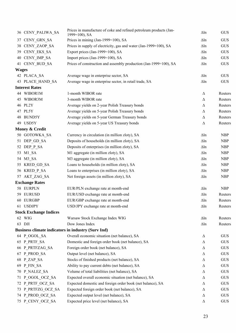
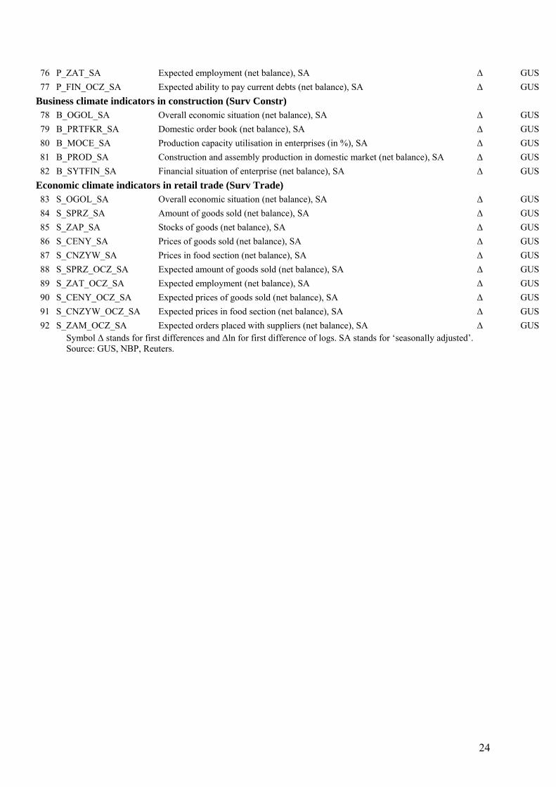
4. Description of data

The data used in the study are monthly data and encompass the period from February

1999 to April 2007 (99 observations). In total, 92 time series were considered, representing of

the basic macroeconomic categories: output and sales, construction, foreign trade, labour

market, prices, wages, interest rates, monetary aggregates, exchange rates, stock exchange

indices and indicators of economic climate in industry, construction and retail trade. The full

list of the variables with the source of the obtained data is presented in Appendix A.

Before embarking on the work on factor model specification the data had to be

appropriately modified. First, all variables were logarithmised, apart from these which

9

contained negative values or were already expressed in the form of fractions (e.g. interest

rates). In the next step, the variables which displayed a clear pattern of seasonality were

adjusted for the impact of seasonal fluctuations using the ARIMAX12 procedure. At this

stage outliers were also removed.

In line with the factor model assumptions (see Stock & Watson [1998]), all the

explanatory variables should be stationary. That’s why variables integrated of order one were

made stationary by taking first differences. It was arbitrarily assumed that all variables

expressing prices and monetary aggregates are I(1). Therefore, they will be featuring in the

model in the form of first differences. Unit root test was preformed for the remaining

variables and appropriate transformation was carried out according to test results. Detailed

information on how each variable was transformed can be found in Appendix A.

In the final step, all variables were standardised to have zero mean and unit standard

deviation.

5. Forecasting from the factor model

The purpose of the present study is to evaluate the applicability of the factor model to

forecasting future values of inflation (CPI). A forecasting horizon of h=1 and h=3 periods was

considered in the study. The forecast applies to a variable constructed in line with the

following formula

hCPICPI

y ththht

)ln( ++ = ,

where CPIt stands for the seasonally adjusted consumer price index with a constant base.

Thus variable hhty + expresses an average monthly relative change in period h.

Forecasts in the dynamic factor model were based on equation (2), which after

estimating common factors and parameters included in polynomials β(L) and γ(L) has the

following from

∑∑=

+−=

+−+ ++=P

pptph

K

kktkhh

hht yγFβαy

11,

11, ˆˆˆˆˆ , (11)

where hhty +ˆ stands for the forecast of variable h

hty + , )ln( 1−= ttt CPICPIy represents monthly

rate of inflation and tF̂ expresses the estimate of the factors vector obtained using the

principal components method as described in point 3. The maximum lags K and P in model

(11) were determined on the basis of indications of the Bayesian information criterion (BIC).

10

The forecasts at moment t+h obtained from equation (11) are determined directly on

the basis of information available in period t. This is a different approach than the iterative

method which in practice is used more often. This method involves determining forecasts for

one period ahead, substituting the obtained forecasts of period t+1 to the model in place of

unknown actual values of explanatory variables in period t+1, re-determining one-period

forecasts for period t+2, substituting the obtained forecasts to the model and so on until the

forecast values for period t+h are obtained.

Direct forecasting for h periods ahead has an advantage over such iterative one-period

forecasting in that it does not require the knowledge of the values of explanatory variables in

the forecasting period and so does not necessitate additional model equation to be constructed

with a view to forecast future values of factors tF̂ . This is obviously just the question of

forecasts prepared for 3 periods ahead, as for h=1 both the forecasting methods are identical.

The forecasting performance of the factor model were evaluated by comparing the

accuracy of inflation forecasts hhty + obtained on the basis of the factor model with the

accuracy of inflation forecasts derived from other competitive models. Three competitive

models have been taken into consideration: a univariate autoregressive model, a model with a

leading indicator and a VAR model with three variables. Brief characteristics of each of these

models are presented below.

Autoregressive model (AR model)

A univariate autoregressive model was adopted as the main benchmark model for

evaluating the forecasting performance of the factor model. In this model the forecast of

variable hhty + are determined according to the formula

∑=

+−+ +=P

pptphh

hht yγαy

11,ˆˆˆ , (12)

where the value of the maximum lag P is set on the basis of the indication of the BIC.

Analogically as in the factor model, forecasts derived from the autoregressive model are

determined directly for h periods ahead.

Autoregressive model with leading indicator (AR-IND)

The second competitive model is a univariate model which apart from current and

lagged values of variable yt as an explanatory variable also contains an leading indicator taken

from GUS (Polish CSO) monthly survey studies of enterprises involved in retail trade. The

11

indicator has the form of the balance of responses to the question on the change of current

prices of goods sold by enterprises in retail trade sector2. In our opinion, out of all the

business climate indicators expressing the response of enterprises to the question of current

and future price level, the selected indicator best corresponds to those price categories which

are covered by the forecast variable, i.e. the Consumer Price Index.

The forecasts from the autoregressive model with the leading indicator are determined

according to the following formula

∑∑=

+−=

+−+ ++=P

pptph

K

kktkhh

hht yγRETPδαy

11,

11, ˆˆˆ , (13)

where variable RETPt expresses a seasonally adjusted value of the balance of responses to the

question on the level of prices in retail trade. In order to establish the lag orders K and P, we

once again make use of the information criterion, the BIC. The forecasts of variable hhty + , just

like in the two previous models, are prepared directly for h periods ahead.

Vector autoregressive model (VAR)

The last model used in this study to compare the accuracy of inflation forecasts

obtained from the factor model is a small model VAR model. The model features three

variables expressing: the Consumer Price Index, industrial production and yields on two-year

Treasury bonds3. All the three variables were expressed in the form of first differences and so

they assumed the same form as in the factor model. The time series of production and prices

had been previously seasonally adjusted.

The equation describing price changes in the VAR model may be noted in the

following form

∑∑∑=

+−=

+−=

+−+ +++=K

kktk

K

kktk

K

kktkt yieldδipγyβαy

11

11

111 ∆ˆ∆ˆˆˆˆ , (14)

where variables ∆ipt and ∆yieldt represent monthly changes in industrial production and

yields on two-year bonds, respectively. For each equation and each variables in the VAR

model the same lag was assumed, which was determined on the basis of BIC indications.

In contrast to other models, the forecasts of variable yt in the VAR model are derived

as one-step ahead forecasts. Thus, for the forecast horizon h=3 periods we make forecasts of

all the three variables in the model for one period ahead and then the forecasts are substituted 2 A detailed description of the indicator’s structure and the actual survey sent to enterprises can be found in Business tendency survey in manufacturing, construction, retail trade, and services – a material cyclically published by the GUS. 3 Analogical set of variables for a VAR model was proposed by Artis et al. [2005] and Stock & Watson [2002a].

12

in place of unknown actual values of those variables and once again determine one-period

forecast for the next period. By reiterating this procedure we arrive at a sequence of one-

period forecasts of variable yt, which we subsequently sum up to obtain values comparable

with the forecast made directly for h periods ahead, as it is the case in the remaining models.

The forecasts computed from the four models were constructed in such a way as to

best simulate the real-time forecasting process. The sample on which the study was based was

divided into two sub-samples. Preliminary specification of all the models was made for data

encompassing the period from February 1999 to March 2005 (for h=3) or to May 2005 (for

h=1), in particular the Bayesian information criterion, BIC was used to determine the dynamic

structure of the models (the lag order) and their parameters were estimated. Observations

from the second part of the sample were used to evaluate the forecasts accuracy. The forecasts

were derived for one and for three months ahead, while after each forecast computation the

sample was lengthened with another observation, the dynamic structure of models was

established using the BIC, data were standardised (for the factor model) and model

parameters and factors were re-estimated. In total, 24 forecasts for each forecast horizon were

determined.

Two different criteria were applied to evaluate the forecasting performance of the

discussed models. The first criterion is the value of the mean square error. For each of the

three competitive models this error was determined in the relative form, i.e. as the ratio of the

mean square error for a given model and the mean square error for the factor model. Values

above one point to better forecasting performance of the factor model. The values of relative

mean square errors are supplemented with the results of West test [2005], which verifies the

hypothesis assuming that the mean square error for a given competitive model is the same as

for the factor model.

The second criterion for evaluating forecast accuracy is based on the results of a test

proposed by Chong & Hendry [1986]. The test involves an estimation of the parameters of the

following regression equation

hht

hBENCHht

hDFMht

hht vyyy ++++ +−+= ,, ˆ)1(ˆ αα , (15)

and subsequent verification of relevant hypotheses against the values of coefficient α. In

equation (15) hhty + stands for the actual rate of inflation (change in prices of consumer goods

and services) in period t+h, hDFMhty ,ˆ + expresses an inflation forecast based on the factor model,

13

while hBENCHhty ,ˆ + stands for a forecast based on a competitive model, both forecasts being made

at moment t for h periods ahead. If coefficient α equals 1, then we say that the inflation

forecast based on the factor model encompasses the forecast from the competitive model. In

contrast, if α is equal to 0, then the forecast based on the competitive model encompasses the

forecast obtained from the factor model. Thus, the verification will test two hypotheses

(1) H0: α = 1 vs H0: α ≠ 1,

and

(2) H0: α = 0 vs H0: α ≠ 0,

The failure to reject the first null-hypothesis (α = 1) and the rejection of the second null-

hypothesis (α = 0) allow concluding that forecasts obtained from the factor model are closer

to the actual values of the forecast variable than those obtained from the competitive model.

6. Empirical results

The first stage of the study involved the determination of the actual number of factors

in the considered factor model. On the basis of the full sample encompassing the period from

February 1999 to April 2007 the eigenvalues of the matrix of correlations for the whole data

set were determined. Analysis of the eigenvalues presented in Table 1 leads to the conclusion

that the model is relatively well fitted to actual data. The first 2 factors explain almost 22% of

the total variance, the first 6 factors approx. 40% and the first 12 factors – almost 58% of the

variance.

The differences between the first and second eigenvalue and between the second and

third eigenvalue amount to 0.051 and 0.028, respectively and are markedly higher than the

differences between subsequent eigenvalues (the difference between the third and fourth

eigenvalue is only 0.007), which would suggest that the number of factors in the model may

be equal to 2 or 3.

The values of information criteria defined by formulas (10a) – (10c) do not yield

unequivocal results. The first two criteria reach minimum for the number of factors equal to 2,

while the third criteria assumes its lowest value for 12 factors. Due to the fact that two out of

three criteria display the same value, we arbitrarily assume that the number of factors in the

model is 2. This value remains consistent with previous observations on the behaviour of

subsequent eigenvalues of the correlation matrix.

14

Table 1. Selection of the number of factors in the model.

(1) (2) (3) (4) (5) (6) (7)

Number of

factors Eigenvalues Contribution

to variance Cumulative

contribution to variance

IC1 IC2 IC3

1 12.537 0.133 -0.065 -0.052 -0.0972 7.765 0.083 0.216 -0.087 -0.060 -0.1513 5.151 0.055 0.271 -0.081 -0.039 -0.1764 4.474 0.048 0.318 -0.069 -0.014 -0.1975 4.061 0.043 0.362 -0.056 0.013 -0.2156 3.572 0.038 0.400 -0.038 0.044 -0.2307 3.247 0.035 0.434 -0.019 0.078 -0.2428 3.117 0.033 0.467 -0.001 0.110 -0.2569 2.932 0.031 0.498 0.017 0.141 -0.270

10 2.671 0.028 0.527 0.038 0.175 -0.28111 2.465 0.026 0.553 0.059 0.210 -0.29212 2.248 0.024 0.577 0.082 0.247 -0.301

Column (2) presents, in descending order, 12 greatest eigenvalues of the correlation matrix. Column (3) contains contributions of particular factors in total variance, while column (4) shows cumulative contributions. The last three columns of the tables express values of information criteria defined by formulas (10a) –(10c). The minimum values of the criteria are highlighted in bold type. Source: Own calculations.

As it was mentioned before, factors estimated using the principal components method

do not have an economic interpretation. However, they span the same space as the structural

factors. For this reason, it is possible to carry out a regression of particular variables against

each of the estimated factors and check which factor explains the behaviour of a given

variable to the greatest extent.

Charts 1a – 1f present the R-squared on the regression of particular variables grouped

in specific economic categories (according to the description in Appendix B) against each of

the first six factors.

The values indicated in the chart suggest that the first factor primarily affects the

variability of prices and domestic interest rates. The second factor determines the

development of the values of industrial production, retail sales, business climate indicators

(mainly from the sector of retails trade) and, once again, domestic interest rates. The third

factor to the greatest extent influences the values of foreign interest rates, the exchange rate,

foreign trade turnover (exports and imports), stock exchange indices and some indicators of

business climate in industry. The fourth of the estimated factors is primarily responsible for

the behaviour of monetary aggregates and, similarly to the third factor, for foreign trade

turnover. The impact of the fifth factor is mostly visible in the case of business climate

indicators in construction and in labour market variables (particularly employment). Finally,

15

the sixth factor loads the variable expressing wages in the enterprises sector and some

indicators of business climate in industry and retail trade.

The interpretation of the first factor as “the driving force” behind price processes in

the economy is to a large extent the result of a relatively strong representation of the price

category in the entire variable set (as many as 27 series). In turn, variables expressing

production are connected with as many as three factors (from the second to the fourth). The

connection of some categories (e.g. construction) with the first six factors is rather weak,

which indicates that a greater impact on the behaviour of these categories is exerted by the

remaining factors, not featured in the charts.

In the further stage of the study the forecasting performance of the factor model were

evaluated. The accuracy of inflation forecasts obtained from the factor model and three

competitive models was compared using two different criteria described in point 5 above. The

forecasts were determined recursively. In the first step, a specification was performed for all

the four models for the sample encompassing the period from February 1999 to March 2005

(for h=3) or to May 2005 (for h=1), in particular the BIC was used to determine the dynamic

structure of each of the models. In the case of the factor model the following general form of

the model was used, which was corresponding to equation (11):

∑∑∑∑=

+−=

+−=

+−=

+−+ ++++=4

11,

3

1

)3(1

)3(,

3

1

)2(1

)2(,

3

1

)1(1

)1(, ˆˆˆˆˆˆˆˆˆ

pptjh

nntnh

mmtmh

kktkhh

hht yγFβFβFβαy , (16)

where )(ˆ itF expresses the estimate of i-th factor in period t. It follows from formula (16) that

in model specification only the first three factors, each one with three lags, and the values of

monthly inflation with a maximum lag of 4 were considered. Artis et al. [2005] emphasise

that forecasting performance of factor models are better if they contain an autoregressive

component and so it was assumed that the model includes at least on lag of variable yt.

Based on the BIC the specification of three competitive models, defined by formulas

(12) – (14), was also carried out. Estimation results of all the models for the last iteration, i.e.

based on the entire sample, are presented in Table 2 below.

16

Table 2. Model estimation results for entire sample.

Forecast horizon h=1 h=3 Sample 02.1999 – 04.2007 02.1999 – 02.2007

DFM model DFM model Constant 0.0040 Constant 0.0040

[8.853] [10.916] yt–1 -0.3319 yt–3 -0.3650

-[2.539] [-3.415] )1(1

ˆ−tF 0.00105 )1(

3ˆ−tF 0.00097

[8.085] [9.017] )2(

1ˆ−tF 0.00024 )2(

3ˆ−tF 0.00018

[3.127] [2.804] R2 0.650 R2 0.678

AR model AR model Constant 0.0012 Constant 0.0007

[3.094] [2.046] yt–1 0.6020 yt–3 0.3021

[7.452] [3.692] yt–4 0.1058 [1.189] yt–5 0.0810 [0.910] yt–6 0.2345 [2.903]

R2 0.353 R2 0.490 AR-IND model AR-IND model

Constant 0.0012 Constant 0.0007 [3.330] [2.099]

yt–1 0.5851 yt–3 0.2803 [7.443] [3.526]

RETPt-1 0.0007 yt–4 0.0709 [2.657] [0.815] yt–5 0.1353 [1.531] yt–6 0.2358 [3.022] RETPt-3 0.0006 [2.668]

R2 0.410 R2 0.529 VAR model VAR model

Constant 0.0013 Constant 0.0013 [3.448] [3.427]

yt–1 0.5554 yt–1 0.5556 [6.593] [6.526]

∆ipt–1 0.0004 ∆ipt–1 0.0004 [1.288] [1.288]

∆yieldt–1 0.0007 ∆yieldt–1 0.0007 [2.239] [2.219]

R2 0.415 R2 0.415

17

In the above table, )(ˆ itF expresses the estimate of i-th factor in period t, variable yt represents monthly rate of

inflation, RETPt stands for seasonally adjusted balance of responses to the question on the level of prices in retail trade, while variables ∆ipt and ∆yieldt correspond to monthly changes in industrial production and yields on 2-year bonds, respectively. Square brackets show the values of t statistics. Source: Own calculations.

It should be noted that in the case of the factor model the BIC revealed the same form

of the model for both considered forecast horizons, i.e. for h=1 and for h=3, which features

only current values of the first two factors (and as h>0 they are in fact lagged by 1 and 3

periods, respectively) and the current value of monthly inflation (in fact lagged by 1 and 3

periods).

On the basis of the obtained models the forecast were produced for h=1 and h=3

periods ahead, on each occasion extending the sample by one observations, once again

specifying the structure of the models and re-estimating factors and parameters of the models.

In total, 24 forecasts of inflation were produced for each forecast horizon, encompassing the

period from June 2005 to May 2007. Table 3 presents the values of relative mean square

errors for each of the models together with West test [2005] results and the results of

verification of two hypothesis assuming that coefficient α in equation (15) is equal to 0 and 1,

respectively. The rejection of the first hypothesis and the failure to reject the second one

means that the factor model has better forecasting performance than the competitive model.

For h=1 the values of mean square errors for all three competitive models expressed in

relation to the mean square error for the factor model are significantly higher than 1. For each

of the considered competitive models the results of West test [2005] confirm that, at the 10%

significance level, we should reject the hypothesis that the values of mean square errors for

this model and the factor model are identical. This means that the factor model has better

forecast accuracy than the remaining models. Moreover, the best of the competitive models

generates forecasts whose mean square error is 67% larger than the error of the factor model,

which may be assessed as a rather high value.

Results of verification of hypotheses for equation (15) indicate that in the case of all

three competitive models at the significance level of 5% we can not reject the hypothesis that

the value of coefficient α equal one, while the hypothesis that this coefficient is equal to zero

should be rejected. Such a result attests to better forecasting performance of the factor model

in comparison to the other models.

18

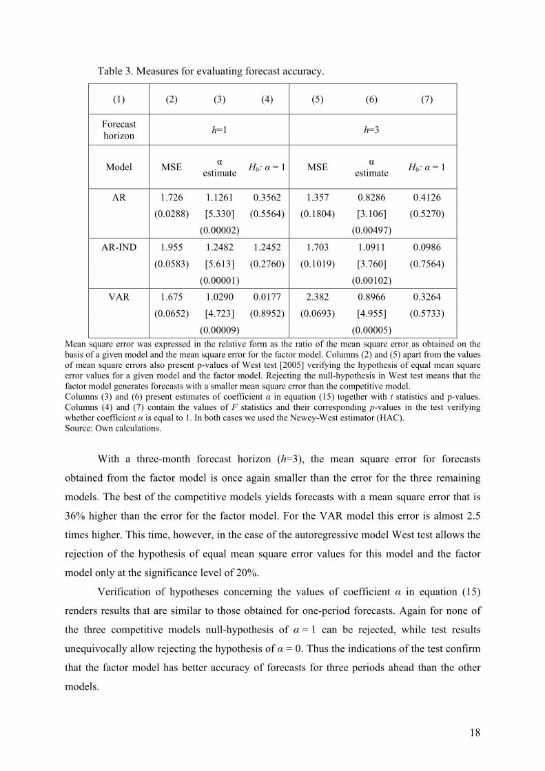
Table 3. Measures for evaluating forecast accuracy.

(1) (2) (3) (4) (5) (6) (7)

Forecast horizon h=1 h=3

Model MSE α estimate H0: α = 1 MSE α

estimate H0: α = 1

AR 1.726 1.1261 0.3562 1.357 0.8286 0.4126 (0.0288) [5.330] (0.5564) (0.1804) [3.106] (0.5270) (0.00002) (0.00497)

AR-IND 1.955 1.2482 1.2452 1.703 1.0911 0.0986

(0.0583) [5.613] (0.2760) (0.1019) [3.760] (0.7564)

(0.00001) (0.00102) VAR 1.675 1.0290 0.0177 2.382 0.8966 0.3264

(0.0652) [4.723] (0.8952) (0.0693) [4.955] (0.5733)

(0.00009) (0.00005) Mean square error was expressed in the relative form as the ratio of the mean square error as obtained on the basis of a given model and the mean square error for the factor model. Columns (2) and (5) apart from the values of mean square errors also present p-values of West test [2005] verifying the hypothesis of equal mean square error values for a given model and the factor model. Rejecting the null-hypothesis in West test means that the factor model generates forecasts with a smaller mean square error than the competitive model. Columns (3) and (6) present estimates of coefficient α in equation (15) together with t statistics and p-values. Columns (4) and (7) contain the values of F statistics and their corresponding p-values in the test verifying whether coefficient α is equal to 1. In both cases we used the Newey-West estimator (HAC). Source: Own calculations.

With a three-month forecast horizon (h=3), the mean square error for forecasts

obtained from the factor model is once again smaller than the error for the three remaining

models. The best of the competitive models yields forecasts with a mean square error that is

36% higher than the error for the factor model. For the VAR model this error is almost 2.5

times higher. This time, however, in the case of the autoregressive model West test allows the

rejection of the hypothesis of equal mean square error values for this model and the factor

model only at the significance level of 20%.

Verification of hypotheses concerning the values of coefficient α in equation (15)

renders results that are similar to those obtained for one-period forecasts. Again for none of

the three competitive models null-hypothesis of α = 1 can be rejected, while test results

unequivocally allow rejecting the hypothesis of α = 0. Thus the indications of the test confirm

that the factor model has better accuracy of forecasts for three periods ahead than the other

models.

19

Out of the remaining models for h=1 the VAR model yields the smallest forecast error,

while for h=3 the most accurate forecast can be obtained from the autoregressive (AR) model.

Summary

This study presents the results of evaluation the forecasting performance of dynamic

factor models in forecasting inflation in the Polish economy. The model was specified on

monthly data encompassing the period from February 1998 to April 2007, while model

parameters and factors were estimated using the principal components method, firstly

proposed by Stock & Watson [1998].

The results confirm that for a one- and three- month horizon the forecasts obtained

from the factor model have smaller mean square error than forecasts based on the competitive

models: an autoregressive model, a model with a leading indicator and a small VAR model.

The advantage of the factor model is more conspicuous in the case of one-month ahead

forecasts, which is also indicated by the results of West test [2005]. With a one-month

forecast horizon, the mean square error in the best-performing competitive model is 67%

higher than in the factor model, while for a three-month horizon this discrepancy is equal to

36%.

Good forecasting performance of the factor model were also confirmed through

verifying hypotheses concerning the coefficients of a regression equation where the actual

values of a forecast variable were described by forecasts based on the factor model and one of

the competitive models. For both forecast horizons and all considered competitive models the

results of statistical tests indicated that we can not reject the hypothesis that coefficient value

for a factor model forecast equals 1. At the same time we should reject the hypothesis of a

zero value of this coefficient.

In the study we tried to associate the estimated factors with particular variables

grouped in appropriate economic categories. Based on the analysis of eigenvalues of a matrix

of correlation of the entire data set and indications of information criteria it was established

that the number of unobserved factors in the model was equal to 2. The first of the factors is

primarily responsible for the behaviour of prices and domestic interest rates. In turn, the

second factor loads mostly production, money and some business climate indicators.

However, it has to be borne in mind that factors determined using the principal components

method are not the structural factors but are only their linear combination and so the estimated

factors should be interpreted with proper caution.

20

Bibliography

1. Armah, N.A., Swanson, N.R. [2007], Seeing inside the Black Box: Using Diffusion Index

Methodology to Construct Factor Proxies in Largescale Macroeconomic Time Series

Environments, mimeo.

2. Altissimo, F., A. Bassanetti, R. Cristadoro, M. Forni, M. Hallin, M. Lippi, L. Reichlin,

[2001], EuroCOIN: a real time coincident indicator of the euro area business cycle, CEPR

Working Paper nr 3108.

3. Artis, M. J., A. Banerjee, M. Marcellino [2005], Factor forecasts for the UK, Journal of

Forecasting, nr 24(4), pp. 279-298.

4. Bai, J. [2003], Inferential theory for factor models of large dimensions, Econometrica, nr

71, pp. 135-171.

5. Bai, J., S. Ng [2002], Determining the number of factors in approximate factor models,

Econometrica, nr 70 pp. 191-221.

6. Bernanke, B., J. Boivin, and P. Eliasz [2005], Measuring Monetary Policy: A Factor

Augmented Vector Autoregressive (FAVAR) Approach, Quarterly Journal of Economics,

nr 120(1), pp. 387-422.

7. Breitung, J., S. Eickmeier [2006], Dynamic factor models, w: O. Hübler, J. Frohn (ed.),

Modern econometric analysis, ch. 3, Springer 2006.

8. Chong, Y.Y, D.F. Hendry [1986], Econometric Evaluation of Linear Macro-economic

Models, Review of Economic Studies, nr 53, pp. 671-690.

9. Eickmeier, S. [2004], Business cycle transmission from the US to Germany – a structural

factor approach, Bundesbank Discussion Paper nr 12/2004.

10. Engle, R.F., M.W. Watson [1981], A One-Factor Multivariate Time Series Model of

Metropolitan Wage Rates, Journal of the American Statistical Association, nr 76, pp. 774-

781.

11. Forni, M., M. Hallin, M. Lippi, L. Reichlin [2005], The generalized dynamic factor

model: one sided estimation and forecasting, Journal of the American Statistical

Association, nr 100, pp. 830-840.

12. Geweke, J. [1977], The dynamic factor analysis of economic time series, ch. 19 w:

Aigner, D.J., A.S. Goldberger (ed.), Latent variables in socio-economic models,

Amsterdam: North Holland.

13. Kapetanios, G., M. Marcellino [2004], A parametric estimation method for dynamic factor

models of large dimensions, Queen Mary University of London Working Paper nr 489.

21

14. Sargent, T., C. Sims [1977], Business cycle modelling without pretending to have too

much a-priori economic theory, w: C. Sims (ed.), New methods in business cycle research,

Minneapolis: Federal Reserve Bank of Minneapolis.

15. Stock, J., and M. Watson [1991], A Probability Model of the Coincident Economic

Indicators, w: K. Lahiri, G.H. Moore (ed.), Leading Economic Indicators: New

Approaches and Forecasting Records, ch. 4., New York, Cambridge University Press, pp.

63-85.

16. Stock, J., M. Watson [1998], Diffusion Indexes, Working Paper nr 6702, National Bureau

of Economic Research.

17. Stock, J., M. Watson [2002a], Macroeconomic forecasting using diffusion indexes,

Journal of Business and Economic Statistics, nr 20, pp. 147-162.

18. Stock, J., M. Watson [2002b]. Forecasting using principal components from a large

number of predictors, Journal of the American Statistical Association nr 97, pp. 1167-

1179.

19. Stock, J., M. Watson [2005], Implications of Dynamic Factor Models for VAR Analysis,

Working Paper nr 11467, National Bureau of Economic Research.

20. West, K. D. [2005], Forecast Evaluation, w: Handbook of Economic Forecasting, G.

Elliott, C.W.J. Granger and A. Timmermann (ed), North Holland Press, Amsterdam.

22

APPENDIX A. Set of variables featured in the study.

No. Name of variable Description of variable Transformation performed

Source of data

Output & Sales 1 PSPM Industrial production in constant prices (Jan-1999=100), SA ∆ln GUS 2 PSPP Industrial production in manufacturing in constant prices (Jan-1999=100),

SA ∆ln GUS 3 PSGRN Production in mining in constant prices (Jan-1999=100), SA ∆ln GUS 4 PZAOP Supply of electricity, gas and water in constant prices (Jan-1999=100), SA ∆ln GUS 5 SPDET Retail sales in constant prices (Jan-1999=100), SA ∆ln GUS

Construction 6 PBUD_SA Construction and assembly production in constant prices (Jan-1999=100),

SA ∆ln GUS 7 L_MIESZK_SA Number of completed dwellings, SA ∆ln GUS

Foreign Trade 8 EKS_SA Exports in constant prices (Jan-1999=100), SA ∆ln GUS 9 IMP_SA Imports in constant prices (Jan-1999=100), SA ∆ln GUS

10 IMP_ROPA Oil imports ∆ln GUS Labour market 11 ZAT_SA Average employment in enterprise sector, SA ∆ln GUS 12 L_BEZ_SA Number of unemployed, SA ∆ln GUS 13 NOWI_BEZ_SA Number of new unemployed, SA ∆ln GUS 14 OFERTY_PRACY_SA Number of vacancies, SA ∆ln GUS

Prices 15 CPI_SA Consumer Price Index (Jan-1999=100), SA ∆ln GUS 16 CENY_ZM_SA CPI net of most volatile prices (Jan-1999=100), SA ∆ln NBP 17 CENY_ZMPAL_SA CPI net of most volatile prices and fuels (Jan-1999=100), SA ∆ln NBP 18 CENY_KONTR_SA CPI net of regulated prices (Jan-1999=100), SA ∆ln NBP 19 CENY_15_SA 15% trimmed mean (Jan-1999=100), SA ∆ln NBP 20 CENY_NETTO_SA Net inflation (Jan-1999=100), SA ∆ln NBP 21 CENY_ZYWN_SA Food prices in CPI basket (Jan-1999=100), SA ∆ln GUS 22 CENY_ALK_SA Alcohol prices in CPI basket (Jan-1999=100), SA ∆ln GUS 23 CENY_TYTON_SA Tobacco prices in CPI basket (Jan-1999=100), SA ∆ln GUS 24 CENY_ODZIEZ_SA Clothes prices in CPI basket (Jan-1999=100), SA ∆ln GUS 25 CENY_OBUWIE_SA Footwear prices in CPI basket (Jan-1999=100), SA ∆ln GUS 26 CENY_MIESZUZ_SA Housing maintenance prices in CPI basket (Jan-1999=100), SA ∆ln GUS 27 CENY_MIESZWYP_SA Home furnishing prices in CPI basket (Jan-1999=100), SA ∆ln GUS 28 CENY_ZDROWIE_SA Health-related prices in CPI basket (Jan-1999=100), SA ∆ln GUS 29 CENY_TRANSP_SA Transport prices in CPI basket (Jan-1999=100), SA ∆ln GUS 30 CENY_LACZN_SA Telecommunications prices in CPI basket (Jan-1999=100), SA ∆ln GUS 31 CENY_KULT_SA Culture-related prices in CPI basket (Jan-1999=100), SA ∆ln GUS 32 CENY_EDUK_SA Education-related prices in CPI basket (Jan-1999=100), SA ∆ln GUS 33 CENY_REST_SA Prices in ‘Hotels and restaurants’ category in CPI basket (Jan-1999=100),

SA ∆ln GUS 34 CENY_PPI_SA Producer prices in industry (Jan-1999=100), SA ∆ln GUS 35 CENY_PRZET_SA Producer prices in manufacturing (Jan-1999=100), SA ∆ln GUS

23

36 CENY_PALIWA_SA Prices in manufacture of coke and refined petroleum products (Jan-1999=100), SA ∆ln GUS

37 CENY_GRN_SA Prices in mining (Jan-1999=100), SA ∆ln GUS 38 CENY_ZAOP_SA Prices in supply of electricity, gas and water (Jan-1999=100), SA ∆ln GUS 39 CENY_EKS_SA Export prices (Jan-1999=100), SA ∆ln GUS 40 CENY_IMP_SA Import prices (Jan-1999=100), SA ∆ln GUS 41 CENY_BUD_SA Prices of construction and assembly production (Jan-1999=100), SA ∆ln GUS

Wages 42 PLACA_SA Average wage in enterprise sector, SA ∆ln GUS 43 PLACE_HAND_SA Average wage in enterprise sector, in retail trade, SA ∆ln GUS

Interest Rates 44 WIBOR1M 1-month WIBOR rate ∆ Reuters45 WIBOR3M 3-month WIBOR rate ∆ Reuters46 PL2Y Average yields on 2-year Polish Treasury bonds ∆ Reuters47 PL5Y Average yields on 5-year Polish Treasury bonds ∆ Reuters48 BUND5Y Average yields on 5-year German Treasury bonds ∆ Reuters49 USD5Y Average yields on 5-year US Treasury bonds ∆ Reuters

Money & Credit 50 GOTOWKA_SA Currency in circulation (in million zloty), SA ∆ln NBP 51 DEP_GD_SA Deposits of households (in million zloty), SA ∆ln NBP 52 DEP_P_SA Deposits of enterprises (in million zloty), SA ∆ln NBP 53 M1_SA M1 aggregate (in million zloty), SA ∆ln NBP 54 M3_SA M3 aggregate (in million zloty), SA ∆ln NBP 55 KRED_GD_SA Loans to households (in million zloty), SA ∆ln NBP 56 KRED_P_SA Loans to enterprises (in million zloty), SA ∆ln NBP 57 AKT_ZAG_SA Net foreign assets (in million zloty), SA ∆ln NBP

Exchange Rates 58 EURPLN EUR/PLN exchange rate at month-end ∆ln NBP 59 EURUSD EUR/USD exchange rate at month-end ∆ln Reuters60 EURGBP EUR/GBP exchange rate at month-end ∆ln Reuters61 USDJPY USD/JPY exchange rate at month-end ∆ln Reuters

Stock Exchange Indices 62 WIG Warsaw Stock Exchange Index WIG ∆ln Reuters63 DJI Dow Jones Index ∆ln Reuters

Business climate indicators in industry (Surv Ind) 64 P_OGOL_SA Overall economic situation (net balance), SA ∆ GUS 65 P_PRTF_SA Domestic and foreign order book (net balance), SA ∆ GUS 66 P_PRTFZAG_SA Foreign order book (net balance), SA ∆ GUS 67 P_PROD_SA Output level (net balance), SA ∆ GUS 68 P_ZAP_SA Stocks of finished products (net balance), SA ∆ GUS 69 P_FIN_SA Ability to pay current debts (net balance), SA ∆ GUS 70 P_NALEZ_SA Volume of total liabilities (net balance), SA ∆ GUS 71 P_OGOL_OCZ_SA Expected overall economic situation (net balance), SA ∆ GUS 72 P_PRTF_OCZ_SA Expected domestic and foreign order book (net balance), SA ∆ GUS 73 P_PRTFZG_OCZ_SA Expected foreign order book (net balance), SA ∆ GUS 74 P_PROD_OCZ_SA Expected output level (net balance), SA ∆ GUS 75 P_CENY_OCZ_SA Expected price level (net balance), SA ∆ GUS

24

76 P_ZAT_SA Expected employment (net balance), SA ∆ GUS 77 P_FIN_OCZ_SA Expected ability to pay current debts (net balance), SA ∆ GUS

Business climate indicators in construction (Surv Constr) 78 B_OGOL_SA Overall economic situation (net balance), SA ∆ GUS 79 B_PRTFKR_SA Domestic order book (net balance), SA ∆ GUS 80 B_MOCE_SA Production capacity utilisation in enterprises (in %), SA ∆ GUS 81 B_PROD_SA Construction and assembly production in domestic market (net balance), SA ∆ GUS 82 B_SYTFIN_SA Financial situation of enterprise (net balance), SA ∆ GUS

Economic climate indicators in retail trade (Surv Trade) 83 S_OGOL_SA Overall economic situation (net balance), SA ∆ GUS 84 S_SPRZ_SA Amount of goods sold (net balance), SA ∆ GUS 85 S_ZAP_SA Stocks of goods (net balance), SA ∆ GUS 86 S_CENY_SA Prices of goods sold (net balance), SA ∆ GUS 87 S_CNZYW_SA Prices in food section (net balance), SA ∆ GUS 88 S_SPRZ_OCZ_SA Expected amount of goods sold (net balance), SA ∆ GUS 89 S_ZAT_OCZ_SA Expected employment (net balance), SA ∆ GUS 90 S_CENY_OCZ_SA Expected prices of goods sold (net balance), SA ∆ GUS 91 S_CNZYW_OCZ_SA Expected prices in food section (net balance), SA ∆ GUS 92 S_ZAM_OCZ_SA Expected orders placed with suppliers (net balance), SA ∆ GUS

Symbol ∆ stands for first differences and ∆ln for first difference of logs. SA stands for ‘seasonally adjusted’. Source: GUS, NBP, Reuters.

25

APPENDIX B Figure 1. R-squared from the regression of particular variables on each of the first six factors. a)

b)

c)

F a c t o r 1

0 .0 0

0 .1 0

0 .2 0

0 .3 0

0 .4 0

0 .5 0

0 .6 0

0 .7 0

0 .8 0

0 .9 0

Output&

Sales

Output&

Sales

Constr

uctio

n

Foreign

Trade

Labo

ur

Prices

Prices

Prices

Prices

Prices

Prices

Prices

Prices

Prices

Wages

Intere

st Rate

s

Intere

st Rate

s

Money

&Credit

Money

&Credit

Excha

nge R

ates

Stock I

ndice

s

Surv In

d

Surv In

d

Surv In

d

Surv In

d

Surv In

d

Surv C

onstr

Surv C

onstr

Surv Trad

e

Surv Trad

e

Surv Trad

e

R s

quar

ed

F a c t o r 2

0 . 0 0

0 . 0 5

0 . 1 0

0 . 1 5

0 . 2 0

0 . 2 5

0 . 3 0

0 . 3 5

0 . 4 0

0 . 4 5

Output&

Sales

Output&

Sales

Constr

uctio

n

Foreign

Trade

Labo

ur

Prices

Prices

Prices

Prices

Prices

Prices

Prices

Prices

Prices

Wages

Intere

st Rate

s

Intere

st Rate

s

Money

&Credit

Money

&Credit

Excha

nge R

ates

Stock I

ndice

s

Surv In

d

Surv In

d

Surv In

d

Surv In

d

Surv In

d

Surv C

onstr

Surv C

onstr

Surv Trad

e

Surv Trad

e

Surv Trad

e

R s

quar

ed

F a c t o r 3

0 .0 0

0 .0 5

0 .1 0

0 .1 5

0 .2 0

0 .2 5

0 .3 0

0 .3 5

Output&

Sales

Output&

Sales

Constr

uctio

n

Foreign

Trade

Labo

ur

Prices

Prices

Prices

Prices

Prices

Prices

Prices

Prices

Prices

Wages

Intere

st Rate

s

Intere

st Rate

s

Money

&Credit

Money

&Credit

Excha

nge R

ates

Stock I

ndice

s

Surv In

d

Surv In

d

Surv In

d

Surv In

d

Surv In

d

Surv C

onstr

Surv C

onstr

Surv Trad

e

Surv Trad

e

Surv Trad

e

R s

quar

ed

26

d)

e)

f)

Source: Own calculations.

F a c t o r 4

0 .0 0

0 .0 5

0 .1 0

0 .1 5

0 .2 0

0 .2 5

0 .3 0

0 .3 5

0 .4 0

0 .4 5

0 .5 0

Output&

Sales

Output&

Sales

Constr

uctio

n

Foreign

Trade

Labo

ur

Prices

Prices

Prices

Prices

Prices

Prices

Prices

Prices

Prices

Wag

es

Intere

st Rate

s

Intere

st Rate

s

Money

&Credit

Money

&Credit

Excha

nge R

ates

Stock I

ndice

s

Surv In

d

Surv In

d

Surv In

d

Surv In

d

Surv In

d

Surv C

onstr

Surv C

onstr

Surv Trad

e

Surv Trad

e

Surv Trad

e

R s

quar

ed

F a c t o r 5

0 .0 0

0 .1 0

0 .2 0

0 .3 0

0 .4 0

0 .5 0

0 .6 0

Output&

Sales

Output&

Sales

Constr

uctio

n

Foreign

Trade

Labo

ur

Prices

Prices

Prices

Prices

Prices

Prices

Prices

Prices

Prices

Wag

es

Intere

st Rate

s

Intere

st Rate

s

Money

&Credit

Money

&Credit

Excha

nge R

ates

Stock I

ndice

s

Surv In

d

Surv In

d

Surv In

d

Surv In

d

Surv In

d

Surv C

onstr

Surv C

onstr

Surv Trad

e

Surv Trad

e

Surv Trad

e

R s

quar

ed

F a c t o r 6

0 .0 0

0 .0 2

0 .0 4

0 .0 6

0 .0 8

0 .1 0

0 .1 2

0 .1 4

0 .1 6

0 .1 8

0 .2 0

Output&

Sales

Output&

Sales

Constr

uctio

n

Foreign

Trade

Labo

ur

Prices

Prices

Prices

Prices

Prices

Prices

Prices

Prices

Prices

Wag

es

Intere

st Rate

s

Intere

st Rate

s

Money

&Credit

Money

&Credit

Excha

nge R

ates

Stock I

ndice

s

Surv In

d

Surv In

d

Surv In

d

Surv In

d

Surv In

d

Surv C

onstr

Surv C

onstr

Surv Trad

e

Surv Trad

e

Surv Trad

e

R s

quar

ed