Departamento de F sica de Part culas E-15782 Santiago de ... · Introduction to the AdS/CFT...

Introduction to the AdS/CFT correspondence

Alfonso V. Ramallo ∗

Departamento de Fısica de Partıculas

Universidade de Santiago de Compostela

and

Instituto Galego de Fısica de Altas Enerxıas (IGFAE)

E-15782 Santiago de Compostela, Spain

Abstract

This is a pedagogical introduction to the AdS/CFT correspondence, based on lecturesdelivered by the author at the third IDPASC school. Starting with the conceptual basisof the holographic dualities, the subject is developed emphasizing some concrete topics,which are discussed in detail. A very brief introduction to string theory is provided,containing the minimal ingredients to understand the origin of the AdS/CFT duality.Other topics covered are the holographic calculation of correlation functions, quark-antiquark potentials and transport coefficients.

∗[email protected]

1

arX

iv:1

310.

4319

v3 [

hep-

th]

1 N

ov 2

013

Contents

1 Introduction and motivation 3

2 The anti-de Sitter space 6

2.1 Counting the degrees of freedom in AdS . . . . . . . . . . . . . . . . . . . . 7

3 String theory basics 9

4 Large N expansion in gauge theories 14

5 D-branes 16

6 D-branes and gravity 18

7 The AdS/CFT for N = 4 SU(N) SYM 21

7.1 Conformal symmetry . . . . . . . . . . . . . . . . . . . . . . . . . . . . . . . 22

7.2 Supersymmetry . . . . . . . . . . . . . . . . . . . . . . . . . . . . . . . . . . 23

7.3 Reduction on the S5 . . . . . . . . . . . . . . . . . . . . . . . . . . . . . . . 23

8 A scalar field in AdS 25

8.1 Application to the KK spectrum in AdS5 × S5 . . . . . . . . . . . . . . . . . 27

8.2 Normalizable and non-normalizable modes . . . . . . . . . . . . . . . . . . . 28

8.3 Higher spin fields . . . . . . . . . . . . . . . . . . . . . . . . . . . . . . . . . 29

9 Correlation functions 29

9.1 One-point function . . . . . . . . . . . . . . . . . . . . . . . . . . . . . . . . 30

9.2 Linear response theory . . . . . . . . . . . . . . . . . . . . . . . . . . . . . . 32

9.3 Two-point function for a scalar field . . . . . . . . . . . . . . . . . . . . . . . 33

10 Quark-antiquark potential 37

10.1 Quark-antiquark potential at finite temperature . . . . . . . . . . . . . . . . 42

10.2 Quark-antiquark potential in a confining background . . . . . . . . . . . . . 43

11 Black hole thermodynamics 45

11.1 Application to the Schwarzschild black hole . . . . . . . . . . . . . . . . . . 47

11.2 AdS black hole . . . . . . . . . . . . . . . . . . . . . . . . . . . . . . . . . . 48

11.3 Comparison with field theory . . . . . . . . . . . . . . . . . . . . . . . . . . 50

2

12 Transport coefficients 52

13 Holographic viscosities 56

1 Introduction and motivation

The AdS/CFT correspondence is a duality relating quantum field theory (QFT) and gravity.

More precisely, the correspondence relates the quantum physics of strongly correlated many-

body systems to the classical dynamics of gravity in one higher dimension. This duality

is also referred to as the holographic duality or the gauge/gravity correspondence. In its

original formulation [1–3], the correspondence related a four-dimensional Conformal Field

Theory (CFT) to the geometry of an anti-de Sitter (AdS) space in five dimensions.

In the study of collective phenomena in condensed matter physics it is quite common that

when a system is strongly coupled it reorganizes itself in such a way that new weakly coupled

degrees of freedom emerge dynamically and the system can be better described in terms of

fields representing the emergent excitations. The holographic duality is a new example of this

paradigm. The new (and surprising!) feature is that the emergent fields live in a space with

one extra dimension and that the dual theory is a gravity theory. As we will argue below,

the extra dimension is related to the energy scale of the QFT. The holographic description is

a geometrization of the quantum dynamics of the systems with a large number of degrees of

freedom, which makes manifest that there are deep connections between quantum mechanics

and gravity.

The gauge/gravity duality was discovered in the context of string theory, where it is quite

natural to realize (gauge) field theories on hypersurfaces embedded in a higher dimensional

space, in a theory containing gravity. However, the study of the correspondence has been

extended to include very different domains, such as the analysis of the strong coupling

dynamics of QCD and the electroweak theories, the physics of black holes and quantum

gravity, relativistic hydrodynamics or different applications in condensed matter physics

(holographic superconductors, quantum phase transitions, cold atoms, ...). In these lectures

we will concentrate on some particular topics, trying to present in clear terms the basic

conceptual ideas, as well as the more practical calculational aspects of the subject. For

reviews on the different aspects of the duality see [4–10].

We will start by motivating the duality from the Kadanoff-Wilson renormalization group

approach to the analysis of lattice systems. Let us consider a non-gravitational system in a

lattice with lattice spacing a and hamiltonian given by:

H =∑x,i

Ji(x, a) Oi(x) , (1)

where x denotes the different lattice sites and i labels the different operators Oi. The Ji(x, a)

3

are the coupling constants (or sources) of the operators at the point x of the lattice. Notice

that we have included a second argument in J i, to make clear they correspond to a lattice

spacing a. In the renormalization group approach we coarse grain the lattice by increasing

the lattice spacing and by replacing multiple sites by a single site with the average value

of the lattice variables. In this process the hamiltonian retains its form (1) but different

operators are weighed differently. Accordingly, the couplings Ji(x, a) change in each step.

Suppose that we double the lattice spacing in each step. Then, we would have a succession

of couplings of the type:

Ji(x, a)→ Ji(x, 2a)→ Ji(x, 4a)→ · · · . (2)

Therefore, the couplings acquire in this process a dependence on the scale (the lattice spacing)

and we can write them as Ji(x, u), where u = (a, 2a, 4a, · · · ) is the length scale at which

we probe the system. The evolution of the couplings with the scale is determined by flow

equations of the form:

u∂

∂uJi(x, u) = βi

(Jj(x, u), u

), (3)

where βi is the so-called β-function of the i th coupling constant. At weak coupling the βi’s

can be determined in perturbation theory. At strong coupling the AdS/CFT proposal is

to consider u as an extra dimension. In this picture the succession of lattices at different

values of u are considered as layers of a new higher-dimensional space. Moreover, the sources

Ji(x, u) are regarded as fields in a space with one extra dimension and, accordingly we will

simply write:

Ji(x, u) = φi(x, u) . (4)

The dynamics of the sources φi’s will be governed by some action. Actually, in the AdS/CFT

duality the dynamics of the φi’s is determined by some gravity theory ( i. e. by some

metric). Therefore, one can consider the holographic duality as a geometrization of the

quantum dynamics encoded by the renormalization group. The microscopic couplings of the

field theory in the UV can be identified with the values of the bulk fields at the boundary of

the extra-dimensional space. Thus, one can say that the field theory lives on the boundary

of the higher-dimensional space (see figure 1).

The sources φi of the dual gravity theory must have the same tensor structure of the

corresponding dual operator Oi of field theory, in such a way that the product φiOi is a

scalar. Therefore, a scalar field will be dual to a scalar operator, a vector field Aµ will be

dual to a current Jµ, whereas a spin-two field gµν will be dual to a symmetric second-order

tensor Tµν which can be naturally identified with the energy-momentum tensor Tµν of the

field theory.

The holographic duality raises several conceptual issues which should be addressed in

order to fully understand it. The simplest of these issues is the matching of the degrees of

freedom on both sides of the correspondence. Let us consider a QFT in a d-dimensional

4

UV

IR

u z

J|UV = !|

!

!

!

!

Figure 1: On the left we illustrate the Kadanoff-Wilson renormalization of a lattice system.In the AdS/CFT correspondence the lattices at different scale are considered as the layersof the higher dimensional space represented on the right of the figure.

spacetime (i.e. in d− 1 spatial dimensions plus time). The number of degrees of freedom of

a system is measured by the entropy. On the QFT side the entropy is an extensive quantity.

Therefore, if Rd−1 is (d− 1)-dimensional spatial region, at constant time, its entropy should

be proportional to its volume in d− 1 dimensions:

SQFT ∝ Vol(Rd−1) . (5)

On the gravity side the theory lives in a (d + 1)-dimensional spacetime. How such a higher

dimensional theory can contain the same information as its lower dimensional dual?. The

crucial point to answer this question is the fact that the entropy in quantum gravity is

subextensive. Indeed, in a gravitational theory the entropy in a volume is bounded by the

entropy of a black hole that fits inside the volume and, according to the so-called holographic

principle, the entropy is proportional to the surface of the black hole horizon (and not to

the volume enclosed by the horizon). More concretely, the black hole entropy is given by the

Bekenstein-Hawking formula:

SBH =1

4GN

AH , (6)

where AH is the area of the event horizon and GN is the Newton constant. In order to apply

(6) for our purposes, let Rd be a spatial region in the (d+ 1)-dimension spacetime where the

gravity theory lives and let us assume that Rd is bounded by a (d− 1)-dimensional manifold

Rd−1 ( Rd−1 = ∂Rd). Then, according to (6), the gravitational entropy associated to Rd

scales as:

SGR(Rd) ∝ Area(∂Rd) ∝ Vol(Rd−1) , (7)

which agrees with the QFT behavior (5). In this lectures we will present several refinements

5

of this argument and we will establish a more precise matching of the degrees of freedom of

the two dual theories.

2 The anti-de Sitter space

In general, finding the geometry associated to a given QFT is a very difficult problem.

However, if the theory is at a fixed point of the renormalization group flow (with a vanishing

β-function) it has conformal invariance (is a CFT) and one can easily find such a metric.

Indeed, let us consider a QFT in d spacetime dimensions. The most general metric in

(d+ 1)-dimensions with Poincare invariance in d-dimensions is:

ds2 = Ω2(z) (−dt2 + d~x2 + dz2) , (8)

where z is the coordinate of the extra dimension, ~x = (x1, · · · , xd−1) and Ω(z) is a function

to be determined. If z represents a length scale and the theory is conformal invariant, then

ds2 must be invariant under the transformation:

(t, ~x)→ λ(t, ~x) , z → λz . (9)

Then, by imposing the invariance of the metric (8) under the transformation (9), we obtain

that the function Ω(z) must transform as:

Ω(z)→ λ−1 Ω(z) , (10)

which fixes Ω(z) to be:

Ω(z) =L

z, (11)

where L is a constant. Thus, by plugging the function (11) into the metric (8) we arrive at

the following form of ds2:

ds2 =L2

z2(−dt2 + d~x2 + dz2) , (12)

which is the line element of the AdS space in (d + 1)-dimensions, that we will denote by

AdSd+1. The constant L is a global factor in (12), which we will refer to as the anti-de Sitter

radius. The (conformal) boundary of the AdS space is located at z = 0. Notice that the

metric (12) is singular at z = 0. This means that we will have to introduce a regularization

procedure in order to define quantities in the AdS boundary.

The AdS metric (12) is a solution of the equation of motion of a gravity action of the

type:

I =1

16πGN

∫dd+1x

√−g[− 2Λ + R + c2R

2 + c3R3 + · · · ] , (13)

with GN is the Newton constant, the ci are constants, g = det(gµν), R = gµνRµν is the scalar

curvature and Λ is a cosmological constant. In particular, if c2 = c3 = · · · = 0 the action (13)

6

becomes the Einstein-Hilbert (EH) action of general relativity with a cosmological constant.

In this case the equations of motion are just the Einstein equations:

Rµν −1

2gµν R = −Λgµν . (14)

Taking the trace on both sides of (14), we get that the scalar curvature is given by:

R = gµνRµν = 2d+ 1

d− 1Λ . (15)

Inserting back this result in the Einstein equation (14) we get that the Ricci tensor and the

metric are proportional:

Rµν =2

d− 1Λ gµν . (16)

Therefore the solution of (14) defines an Einstein space. Moreover, the Ricci tensor for the

metric (12) can be computed directly from its definition. We get:

Rµν = − d

L2gµν . (17)

By comparing (16) and (17) we get that the AdSd+1 space solves the equations of motion

(14) of EH gravity with a cosmological constant equal to:

Λ = −d(d− 1)

2L2, (18)

which is negative. It follows from (15) and (18) that the scalar curvature for the AdSd+1

space with radius L is given by:

R = −d(d+ 1)

L2. (19)

In these lectures we will be mostly interested in gauge theories in 3 + 1 dimensions, which

corresponds to taking d = 4 in our formulas. The dual geometry found above for this case

is AdS5. This was precisely the system studied in [1] by Maldacena, who conjectured that

the dual QFT is super Yang-Mills theory with four supersymmetries (N = 4 SYM).

2.1 Counting the degrees of freedom in AdS

After having identified the AdS space as the gravity dual of a field theory with conformal

invariance, we can refine the argument of section 1 to match the number of degrees of freedom

of both sides of the duality.

Let us consider first the QFT side. To regulate the theory we put both a UV and IR

regulator. We place the system in a spatial box of size R (which serves as an IR cutoff) and

we introduce a lattice spacing ε that acts as a UV regulator. In d spacetime dimensions the

7

system has Rd−1/εd−1 cells. Let cQFT be the number of degrees of freedom per lattice site,

which we will refer to as the central charge. Then, the total number of degrees of freedom

of the QFT is:

NQFTdof =

(Rε

)d−1

cQFT . (20)

The central charge is one of the main quantities that characterize a CFT. If the CFT is

a SU(N) gauge field theory, such as the theory with four supersymmetries which will be

described below, the fields are N ×N matrices in the adjoint representation which, for large

N , contain N2 independent components. Thus, in these SU(N) CFT’s the central charge

scales as cSU(N) ∼ N2.

Let us now compute the number of degrees of freedom of the AdSd+1 solution. According

to the holographic principle and to the Bekenstein-Hawking formula (6), the number of

degrees of freedom contained in a certain region is equal to the maximum entropy, given by

NAdSdof =

A∂4GN

, (21)

with A∂ being the area of the region at boundary z → 0 of AdSd+1. Let us evaluate A∂ by

integrating the volume element corresponding to the metric (12) at a slice z = ε→ 0:

A∂ =

∫Rd−1, z=ε

dd−1 x√g =

(Lε

)d−1∫Rd−1

dd−1 x . (22)

The integral on the right-hand-side of (22) is the the volume of Rd−1, which is infinite. As

we did on the QFT side, we regulate it by putting the system in a box of size R:∫Rd−1

dd−1 x = Rd−1 . (23)

Thus, the area of the A∂ is given by:

A∂ =(RLε

)d−1

. (24)

Let us next introduce the Planck length lP and the Planck mass MP for a gravity theory in

d+ 1 dimensions as:

GN = (lP )d−1 =1

(MP )d−1. (25)

Then, the number of degrees of freedom of the AdSd+1 space is:

NAdSdof =

1

4

(Rε

)d−1 ( LlP

)d−1

. (26)

By comparing NQFTdof and NAdS

dof we conclude that they scale in the same way with the IR

and UV cutoffs R and ε and we can identify:

1

4

( LlP

)d−1

= cQFT . (27)

8

This gives the matching condition between gravity and QFT that we were looking for. Notice

that a theory is (semi)classical when the coefficient multiplying its action is large. In this

case the path integral is dominated by a saddle point. The action of our gravity theory

in the AdSd+1 space of radius L contains a factor Ld−1/GN . Thus, taking into account the

definition of the Planck length in (25), we conclude that the classical gravity theory is reliable

if:

classical gravity in AdS→( LlP

)d−1

1 , (28)

which happens when the AdS radius is large in Planck units. Since the scalar curvature

goes like 1/L2, the curvature is small in Planck units. Thus, a QFT has a classical gravity

dual when cQFT is large, or equivalently if there is a large number of degrees of freedom per

unit volume or a large number of species (which corresponds to large N for SU(N) gauge

theories).

3 String theory basics

As mentioned in the introduction, the AdS/CFT correspondence was originally discovered

in the context of string theory. Although it can be formulated without making reference

to its stringy origin, it is however very convenient to know its connection to the theory

of relativistic strings in order to acquire a deep understanding of the duality. We will

start reviewing qualitatively this connection in this section (refs [11–16] contain systematic

expositions of string theory with different levels of technical details).

Counting the degrees of freedom (again)

NQFTdof =

!

R

!

"d!1

cQFTIn SU(N) YM ! cSU(N) " N2

cQFT ! central charge

A! =

!

Rd!1, z="

dd!1 x!

g =

"L

!

#d!1!

Rd!1

dd!1 x

!Rd!1

dd!1

x = Rd!1

A! =

!

RL

!

"d!1

GN = (lP )d!1 =1

(MP )d!1

NAdSdof =

1

4

!

R

!

"d!1 !

L

lP

"d!1

QFT side Put the system in a box of size R with lattice spacing !

# dof per cell

Gravity side

Area of the AdS boundary

Planck length and mass

From the entropy formula

!

L

lP

"d!1

! cQFTclassical gravity in AdS !

!

L

lP

"d!1

>> 1

large # dof per unit volume

String theory basics

Historical origin Description of hadronic resonances of high spin (60’s)

M2! J

M2

J

Regge trajectories

Basic objects extended along some characteristic distance ls

CHAPTER 1 Introduction 13

Strings can be open (Fig. 1.5) or closed (Fig. 1.6), the latter meaning that the ends are connected.

Excitations of the string give different fundamental particles. As a particle moves through space-time, it traces out a world line. As a string moves through space-time, it traces out a worldsheet (see Fig. 1.7), which is a surface in space-time parameterized by ( , )! " . A mapping xµ " !( , ) maps a worldsheet coordinate ( , )! " to the space-time coordinate x.

So, in the world according to string theory, the fundamental objects are tiny strings with a length on the order of the Planck scale (10 33# cm). Like any string,

Figure 1.5 Fundamental particles are extended one-dimensional objects called strings.

Figure 1.6 A closed string has no loose ends.

x

t

Schematic representation of astring moving through space-time, it is represented by aworldsheet (a tube for a closedstring)

x

t

A particle moving throughspace-time has a worldline

Figure 1.7 A comparison of a worldsheet for a closed string and a world line for a point particle. The space-time coordinates of the world line are parameterized as x xµ µ= ( )" , while the space-time coordinates of the worldsheet are parameterized

as xµ( , )" ! where ( , )! " give the coordinates on the surface of the worldsheet.

CHAPTER 1 Introduction 13






x

t


x

t




openclosed

non-local theory

The rotational degree of freedom gives rise to high spins and Regge trajectories

In modern language a meson is a quark-antiquark pair joined by a stringCHAPTER 1 Introduction 13






x

t


x

t




qq E ! L confinement!

d

d

x

x

x

! !!

0

1

2

)!(µx

s

xµ = x

µ(!)

xµ! parametrizes the space in which the point particle is moving

! ! world-line coordinate

Classical relativistic particle

S = !m

!

ds = !m

! !1

!0

d!"

!"µ" xµ x"Action

Figure 2: In a Regge trajectory the mass square M2 of the particles grows linearly with theirspin J .

Historically, string theory was introduced in the sixties as an attempt to describe the

hadronic resonances of high spin observed in the experiments. Experimentally, the mass

9

square of these particles is linearly related to its spin J :

M2 ∼ J . (29)

It is then said that the hadrons are distributed along Regge trajectories (see figure 2).

String theory was introduced to reproduce this behavior. Actually, it is not difficult to verify

qualitatively that the rotational degree of freedom of the relativistic string gives rise to Regge

trajectories as in (29). Indeed, let us suppose that we have an open string with length L

and tension T which is rotating around its center of mass. The mass of this object would

be M ∼ T L, whereas its angular momentum J would be J ∼ P L, with P being its linear

momentum. In a relativistic theory P ∼ M , which implies that J ∼ P L ∼ M L ∼ T−1M2

or, equivalently, M2 ∼ T J . Thus, we reproduce the Regge behavior (29) with the slope

being proportional to the string tension T .

The basic object of string theory is an object extended along some characteristic distance

ls. Therefore, the theory is non-local. It becomes local in the point-like limit in which the

size ls → 0. The rotation degree of freedom of the string gives rise to Regge trajectories

similar to those observed experimentally. In modern language one can regard a meson as a

quark-antiquark pair joined by a string. The energy of such a configuration grows linearly

with the length, and this constitutes a model of confinement.

The classical description of a relativistic string is directly inspired from that of a point

particle in the special theory of relativity. Indeed, let us consider a relativistic point particle

of mass m moving in a flat spacetime with Minkowski metric ηµν . As it moves the particle

describes a curve in spacetime (the so-called worldline), which can be represented by a

function of the type:

xµ = xµ(τ) , (30)

where xµ is the coordinate in the space in which the point particle is moving (the target

space) and τ parameterizes the path of the particle (the worldline coordinate). The action

of the particle is proportional to the integral of the line element along the trajectory in

spacetime, with the coefficient being given by the mass m of the particle:

S = −m∫ds = −m

∫ τ1

τ0

dτ√−ηµν xµ xν . (31)

Let us now consider a relativistic string. A one-dimensional object moving in spacetime

describes a surface (the so-called worldsheet). Let dA be the area element of the worldsheet

(see figure 3). Then, the analogue of the action (31) for a string is the so-called Nambu-Goto

action:

SNG = −T∫

dA , (32)

where T is the tension of the string, given by:

T =1

2πα′, (33)

10

and α′ is the Regge slope (α′ has units of (length)2 or (mass)−2). The string length and

mass are defined as:

ls =√α′ =

1

Ms

. (34)

x0

x1

x2

!

"

dA

Figure 3: The string sweeps in spacetime a two-dimensional worldsheet.

Then, the string tension is related to ls and Ms as:

T =1

2πl2s=

M2s

2π. (35)

Let us write more explicitly the Nambu-Goto action (32). With this purpose we will take

two coordinates ξα (α = 0, 1) to parameterize the worldsheet Σ ( (ξ0, ξ1) = (τ, σ)). Let us

assume that the string moves in a target space M with metric Gµν . The embedding of Σ

in the spacetime M is characterized by a map Σ → M with ξα → Xµ(ξα). The induced

metric on Σ is:

Gαβ ≡ Gµν ∂αXµ ∂βX

ν . (36)

Thus, the Nambu-Goto action of the string is:

SNG = −T∫ √

− det Gαβ d2ξ . (37)

The action (37) depends non-linearly on the embedding functions Xµ(τ, σ). The classical

equations of motion derived from (37) are partial differential equations which, remarkably,

can be solved for a flat target spacetime with Gµν = ηµν , both for Neumann and Dirich-

let boundary conditions. Actually, the functions Xµ(τ, σ) can be represented in a Fourier

expansion as an infinite superposition of oscillation modes, much as in the string of a violin.

The quantization of the string can be carried out by using the standard methods in quan-

tum physics. The simplest way is just by canonical quantization, i.e. by considering that

the Xµ are operators and by imposing canonical commutation relations between coordinates

11

and momenta. As a result one finds that the different oscillation modes can be interpreted

as particles and that the spectrum of the string contains an infinite tower of particles with

growing masses and spins that are organized in Regge trajectories, with 1/ls being the mass

gap.

The close scrutiny of the consistency conditions of the quantum string reveals many sur-

prises (quantizing the string is like opening Pandora’s box!). First of all, the mass spectrum

contains tachyons (particles with m2 < 0), which is a signal of instability. In order to avoid

this problem one must consider a string which has also fermionic coordinates and require that

the system is supersymmetric (i.e. that there is a symmetry between bosonic and fermionic

degrees of freedom). This generalization of the bosonic string (37) is the so-called super-

string. Another consistency requirement imposed by the quantization is that the number D

of dimensions of the space in which the string is moving is fixed. For a superstring D = 10.

This does not mean that the extra dimensions have the same meaning as the ordinary ones

of the four-dimensional Minkowski spacetime. Actually, the extra dimensions should be re-

garded as defining a configuration space (as the phase space in classical mechanics does).

We will see below that this is precisely the interpretation that they have in the context of

the AdS/CFT correspondence.

Another important piece of information about the nature of string theory is obtained

from the analysis of the spectrum of massless particles. Massive particles have a mass

which a multiple of 1/ls and, therefore, they become unobservable in the low-energy limit

ls → 0. Then, after eliminating the tachyons by using supersymmetry, the massless particles

are the low-lying excitations of the spectrum. We must distinguish the case of open and

closed strings. The spectrum of open strings contains massless particles of spin one with the

couplings needed to have gauge symmetry. These particles can be naturally identified with

gauge bosons (photons, gluons,...). The big surprise comes when looking at the spectrum

of closed strings, since it contains a particle of spin two and zero mass which can only be

interpreted as the graviton (the quantum of gravity). Besides, quantum consistency of the

propagation of the string in a curved space implies Einstein equations in ten dimension plus

corrections:

Rµν + · · · = 0 . (38)

Then, one is led to conclude that string theory is not a theory of hadrons but a theory of

quantum gravity!!. Thus, the string length ls should be of the order of the Planck length

lP and not of the order of the hadronic scale ∼ 1 fm). Elementary strings without internal

structure and zero thickness were born for the wrong purpose. Moreover, in addition to the

graviton, the massless spectrum contains antisymmetric tensor fields of the form Aµ1···µp+1 ,

which will become very relevant in formulating the AdS/CFT correspondence.

As strings propagate through the target spaceM, they can suffer interactions by splitting

in two or more parts or by joining with other strings. The worldsheet for one of these

interactions is just a two-dimensional surface with holes and boundaries which can be thought

12

~ gs

Figure 4: A vertex in field theory corresponds to a two-dimensional surface with boundaries(left). The triple vertex for three closed strings is represented on the right as a pants surface.

as a vertex in QFT perturbation theory in which the lines has been thickened, as shown in

figure 4. In closed string theory the basic interaction is a string splitting into two (or the

inverse process of two closed strings merging into one). The corresponding worldsheet has

the form of pants, which can be obtained by thickening a triple vertex in QFT. A loop

in string perturbation theory can be obtained with two triple vertices, which produces a

worldsheet which is a Riemann surface with a hole. Higher order terms in perturbation

theory correspond to having more holes on the worldsheet (see figure 5). Therefore, the

perturbative series in string theory is a topological expansion!. In the topology of two-

dimensional surfaces, the number h of holes (or handles) of the surface is called the genus of

the surface. In string perturbation theory, h is just the number of string loops.

Let us suppose that we weigh every triple vertex with a string coupling constant coupling

gs. It is clear from the discussion above that string perturbation theory is an expansion of

the type:

A =∞∑h=0

g2h−2s Fh(α

′) , (39)

where A is some amplitude. In the next section we will identify a topological expansion in

gauge theories which has the same structure as the series (39).

+ + + . . .

Figure 5: Perturbative expansion of the amplitude corresponding to four closed strings.

13

4 Large N expansion in gauge theories

Let us consider U(N) Yang-Mills theory with lagrangian

L = − 1

g2Tr[FµνF

µν], (40)

where the non-abelian gauge field strength is given by:

Fµν = ∂µAν − ∂νAµ + [Aµ, Aν ] . (41)

In the equations above Aµ is an N×N matrix whose elements can be written as Aaµ , b, where

a, b are indices that run from 1 to N . Let us rewrite L as:

L = −Nλ

Tr[FµνF

µν], (42)

where λ = g2N is the so-called ’t Hooft coupling. The ’t Hooft expansion [17] corresponds

to keeping λ fixed and to perform an expansion of the amplitudes in powers of N . It turns

out that the different powers of N correspond to the different topologies. One can prove this

by adopting a double line notation for the gauge propagator. Then, one can verify that the

color lines form the perimeter of an oriented polygon (a face). Polygons join at a common

edges in such a way that every vacuum graph is associated to a triangulated two-dimensional

surface formed by sewing all polygons along the edges.

Topological expansion of gauge theories

U(N) Yang-Mills theory L = !1

g2Tr

!

Fµ!Fµ!"

Fµ! = !µ A! ! !!Aµ + [Aµ, A! ] Aµ ! N " N matrix Aaµ , b

’t Hooft topological expansion ! in powers of N at fixed !

double line notation

gauge propagatord

a

b

c

vertices!

N

!

!

!

N

index loop ! color sum ! N

Rewrite L L = !N

!Tr

!

Fµ!Fµ!

"

! = g2N ! ’t Hooft coupling

D !

!

!

N

"E !

N

!

"V

NF

= NF!E+V

!E!VF ! number of index loops (faces)

V ! number of vertices

E ! number of propagators (edges) connecting two vertices

Diagram D with

! = 2 ! 2h

The color lines form the perimeter of an oriented polygon (a face)

Polygons join at a common edge

Every vacuum graph is associated to a triangulated 2d surface

h ! genus ! number of handles

F ! E + V = !Power of N Euler characteristic (topological invariant)

Planar diagrams ! h = 0 ! triangulate a sphere ! N2

Non-planar diagrams ! h " 1 ! h-torus # N2!2h

Topological expansion of gauge theories

U(N) Yang-Mills theory L = !1

g2Tr

!

Fµ!Fµ!"

Fµ! = !µ A! ! !!Aµ + [Aµ, A! ] Aµ ! N " N matrix Aaµ , b

’t Hooft topological expansion ! in powers of N at fixed !

double line notation

gauge propagatord

a

b

c

vertices!

N

!

!

!

N

index loop ! color sum ! N

Rewrite L L = !N

!Tr

!

Fµ!Fµ!

"

! = g2N ! ’t Hooft coupling

D !

!

!

N

"E !

N

!

"V

NF

= NF!E+V

!E!VF ! number of index loops (faces)

V ! number of vertices

E ! number of propagators (edges) connecting two vertices

Diagram D with

! = 2 ! 2h

The color lines form the perimeter of an oriented polygon (a face)

Polygons join at a common edge

Every vacuum graph is associated to a triangulated 2d surface

h ! genus ! number of handles

F ! E + V = !Power of N Euler characteristic (topological invariant)

Planar diagrams ! h = 0 ! triangulate a sphere ! N2

Non-planar diagrams ! h " 1 ! h-torus # N2!2h

Figure 6: Gauge propagator and vertices in the double line notation of Yang-Mills U(N)theories.

It is not difficult to find the powers of N and λ appearing in a given diagram D with no

external lines. The contributions of the gauge propagator and the vertices are displayed in

figure 6. Moreover, every index loop contributes with a power of N . Suppose that E is the

number of propagators (edges) of D connecting two vertices, V is the number of vertices and

F is the number of index loops (faces). Then, one can show that:

D ∼( λN

)E (Nλ

)VNF = NF−E+V λE−V . (43)

14

Let us denote by χ the combination of F , E and V that appears in the exponent of N in

(43):

F − E + V = χ , (44)

which is nothing but the Euler characteristic of the triangulation, which only depends on the

topology of the surface. If the diagram triangulates a surface with h handles (an h-torus),

χ is given by:

χ = 2− 2h . (45)

Thus the diagrams are weighed with a power of N determined by the number of handles

of the surface that they triangulate (see figure 7). The planar diagrams are those that can

be drawn on a piece of paper without self-crossing. They correspond to h = 0 and their

contribution is of the type N2λn, for some power n which depends on the diagram considered.

Clearly, as the dependence on N goes like N2−2h the diagrams with h = 0 are the dominant

ones in the large N expansion. For this reason the large N limit is also called the planar

limit of the gauge theory (see [18] for more details and examples).

Figure 7: The planar diagram on the left can be drawn on a sphere, whereas the non-planardiagram on the right must be drawn on a torus.

The effective action Z can be obtained by computing the sum over the connected vacuum-

to-vacuum diagrams. It has the structure:

logZ =∞∑h=0

N2−2h

∞∑l=0

cl,h λl =

∞∑h=0

N2−2h fh(λ) , (46)

where fh(λ) is the sum of Feynman diagrams that can be drawn in a surface of genus h.

This clearly suggest a connection with the perturbative expansion of string theory written

in (39) if one identifies the string coupling constant gs as:

gs ∼1

N. (47)

15

Heuristically one can say that gauge theory diagrams triangulate the worldsheet of an effec-

tive string. The AdS/CFT correspondence is a concrete realization of this connection in the

limit (N, λ)→∞ (i.e. for planar theories in the strongly coupled regime). This dual stringy

description of gauge theory is nothing but a quantum version of the familiar description of

electromagnetism in terms of the string-like lines of force.

5 D-branes

Besides the perturbative structure reviewed above, string theories have a non-perturbative

sector, which plays a crucial role in connecting them with gauge theories. The relevant ob-

jects in this non-perturbative sector are the solitons, which are extended objects. The most

important solitons for the AdS/CFT correspondence are the Dp-branes, that are objects

extended in p+ 1 directions (p spatial + time). The Dp-branes can be defined as hypersur-

faces where strings end (see figure 8). They can be obtained by quantizing the string with

fixed ends along hyperplanes (Dirichlet boundary conditions). In addition, they can also

be understood as objects charged under the antisymmetric tensor fields Aµ1···µp+1 of string

theory, which naturally couple to the Dp-brane worldvolume as:

Aµ1···µp+1 →∫Mp+1

Aµ1···µp+1 dxµ1 · · · dxµp+1 , (48)

with Mp+1 being the worldvolume of the Dp-brane. The Dp-branes are dynamical objects

that can move and get excited. Schematically, their action takes the form:

SDp = −TDp∫dp+1x [· · · ] , (49)

with TDp being the tension of the Dp-brane, which in terms of the string coupling constant

gs and the string length ls is given by:

TDp =1

(2π)p gs lp+1s

. (50)

Notice from (50) that TDp ∼ g−1s , which confirms that the Dp-branes are non-perturbative

objects in string theory. The dependence of TDp on ls in (50) is fixed by dimensional analysis.

The Dp-branes can have two classes of excitations. The first one correspond to rigid

motions and deformations of their shape. These degrees of freedom can be parameterized by

the 9−p coordinates φi (i = 1, · · · , 9−p) transverse to the (p+1)-dimensional worldvolume in

the ten-dimensional target space. The φi’s are just scalar fields on the Dp-brane worldvolume.

Besides, the Dp-branes can have internal excitations. To get a clue on how to represent these

excitations, let us recall that the endpoint of the string is a charge. When there is a charge,

16

SDp = !TDp

!d

p+1x [· · · ]

TDp ! tension of the Dp-brane TDp =1

(2!)p gs lp+1s

The D-branes are dynamical objects

Action

TDp ! g!1s " non-perturbative objects

Excitations of a D-brane

-Deformation of shape and rigid motion

Parametrized by 9 ! p coordinates " !i (i = 1, · · · , 9 ! p)

They are scalar fields on the worldvolume

SDBI = !TDp

!

dp+1x"

!det(gµ! + 2!l2sFµ!)

gµ! = !µ! + (2"l2s)2 #µ$i #!$i

Expanding in powers of Fµ! and !

g2

Y M = 2(2!)p!2 lp!3

s gs

SDBI = !

1

g2

Y M

!

1

4Fµ!Fµ!

+1

2!µ"i !!"i

+ · · ·

"

Aµ

-Internal excitations

Dirac-Born-Infeld action

The endpoint of the string is a charge that sources a gauge field on the worldvolume

gauge+scalars+(fermions)

YM coupling

In flat space

Figure 8: The D-branes are hyperplanes where open strings can end. The endpoints of thestrings source gauge fields Aµ on the D-brane worldvolume.

a gauge field is sourced, as illustrated in figure 8. Then, it follows that a Dp-brane has an

abelian gauge field Aµ (µ = 0, · · · , p) living in its worldvolume. The action of the Dp-brane

which takes into account these two types of excitations is the so-called Dirac-Born-Infeld

action, which can be written as:

SDBI = −TDp∫dp+1x

√− det(gµν + 2π l2s Fµν) , (51)

where gµν is the induced metric on the worldvolume and Fµν = ∂µAν − ∂ν Aµ is the field

strength of the gauge field Aµ. When the worldvolume gauge field is not excited (Fµν = 0)

the DBI action (51) becomes the natural generalization of the Nambu-Goto action (37) for

an object extended along p spatial directions.

Let us consider a Dp-brane in flat space. The induced metric in this case takes the form:

gµν = ηµν + (2πl2s)2 ∂µφ

i ∂νφi , (52)

where the φi are the coordinates that parameterize the embedding of the brane. Let us

now expand the square root of (51) in powers of Fµν and ∂µφ. The quadratic terms in this

expansion can be written as:

S(2)DBI = − 1

g2YM

( 1

4FµνF

µν +1

2∂µφ

i ∂µφi + · · ·), (53)

which is just the ordinary action of a gauge field and 9− p scalar fields. In (53) gYM is the

Yang-Mills coupling, which, in terms of ls and gs, is given by:

g2YM = 2(2π)p−2 lp−3

s gs . (54)

17

In addition to Aµ and φ, in superstring theory the branes have fermionic excitations, which

can be represented in terms of fermionic fields.

We have just discovered one of the most important features of the Dp-branes: they contain

a gauge theory living in their wordlvolume!. In the case of a single Dp-brane the gauge group

is U(1), as in (53). However, if we consider a stack of coincident parallel Dp-branes the gauge

group gets promoted to U(N). Indeed, one can verify in this case that the fields Aµ and φi

are matrices transforming in the adjoint representation of U(N). The non-diagonal elements

of these fields correspond to excitations connecting different branes, whereas the diagonal

ones are excitations on a single brane. Actually, the U(1) component of the U(N) gauge

theory can be decoupled from the SU(N) fields. Therefore, we conclude that a stack of N

Dp-branes realizes a SU(N) gauge theory in p+ 1 dimensions.

The D-branes have brought a completely new perspective on gauge theories which gives

rise to what is called brane engineering. The geometric realization of the gauge symmetry

that they provide allows to perform a series of transformations which lead to discover new

unexpected properties of gauge theories. For example, one can move the branes, place

them in different spaces, etc. In the gauge theory, these transformations lead to dualities,

reductions of the amount of supersymmetry, changes of the field content, etc. In general

we have a novel geometric insight on gauge dynamics. The AdS/CFT correspondence is an

important outcome of this new realization of the gauge symmetry.

The particular case of the D3-branes is specially relevant in what follows. In this case we

have a 3 + 1 worldvolume and 10− 4 = 6 scalar fields. The corresponding four-dimensional

SU(N) gauge theory can be identified with super Yang-Mills theory with four supersymme-

tries (N = 4 SYM). This theory is an exact CFT at the quantum level and will be the basic

example of the AdS/CFT correspondence. Notice from (54) that the Yang-Mills coupling is

dimensionless in this case and is related to the string coupling constant gs as:

g2YM = 4πgs , (D3− branes) . (55)

6 D-branes and gravity

String theory is a gravity theory in which all types of matter distort the spacetime. This

distortion is determined by solving Einstein equations which follow from the action:

S =1

16π G

∫d10x√−g R + · · · . (56)

The ten-dimensional Newton constant in (56) is related to string parameters as:

16π G = (2π)7 g2s l

8s . (57)

18

The dependence of G on ls in (57) follows from dimensional analysis. The dependence on gsfollows by comparing two-to-two scattering amplitudes in string theory and in supergravity

(see figure 9).

~ G~ gs2

gravitonstring

Figure 9: In string theory the exchange of a graviton is obtained as the low-energy limit ofthe exchange of a closed string.

The Dp-branes (and other extended objects) are solutions of the Einstein equations. Let

us consider these solutions at the linearized level of weak gravity (i.e. when we are far from

the object). The linearized metric for a point-like object in a D-dimensional spacetime is:

ds2 ≈ −(1 + 2ϕ) dt2 +(

1− 2

D − 3ϕ)(

dx21 + · · · + dx2

D−1

), (58)

where the function ϕ parameterizes the deviation of the metric from the flat Minkowski metric

in D dimensions. The specific form (58) can be obtained by solving the linearized Einstein

equations and generalizes the standard result in general relativity in four dimensions. As in

this latter particular case, one can identify the function ϕ with the Newtonian gravitational

potential, as seen by comparing the motion along a geodesic and Newton’s law. Thus:

ϕ ∼ GM

rD−3, (59)

where M is the mass of the particle and r =√x2

1 + · · · + x2D−1 is the radial coordinate of

the space. The function ϕ is a solution of the Poisson equation in D− 1 dimensions. Notice

that the power D− 3 is equal to the number dT of dimensions transverse to the object (i. e.

dT = D − 1) minus 2:

D − 3 = dT − 2 . (60)

For an extended object (along p spatial directions) the corresponding linearized metric takes

the form:

ds2 ≈ (1 + 2ϕ)(− dt2 + dx2

1 + · · ·+ dx2p

)+(1− 2(p+ 1)

D − p− 3ϕ)(dx2

p+1 + · · ·+ dx2D−1

). (61)

Since now the number of transverse directions is dT = D − 1− p, the function ϕ must be:

ϕ ∼ GM

rD−p−3. (62)

19

The D3-brane solution is a solution of 10d supergravity corresponding to a stack of N

coincident D3-branes. The (exact) metric takes the form:

ds2 = H−12

(− dt2 + dx2

1 + dx22 + dx2

3

)+H

12 (dr2 + r2dΩ2

5 ) , (63)

with dΩ25 is the line element of a unit S5. Notice that dr2 + r2dΩ2

5 is the flat metric of R6.

The function H(r) is the so-called warp factor:

H = 1 +L4

r4, (64)

with the constant L being given by:

L4 = 4πgsNl4s . (65)

At linearized level (when r → ∞) the solution (63) corresponds to the general solution in

(61) with D = 10, p = 3 and the function φ given by:

ϕ = −1

4

L4

r4. (66)

Comparing this expression of ϕ with the one written in (62) for D = 10 and p = 3 we

conclude that:

GM ∼ L4 . (67)

Let us find this last relation from a different reasoning. As G ∼ g2s l

8s (see (57)) and since M

should be the mass of a stack of N D3-branes with tension TD3 ∼ 1/(gsl4s), we should have:

GM ∼ g2s l

8s

N

gsl4s∼ Ngsl

4s , (68)

which, apart from a numerical factor is precisely the value of L4 written in (65).

The geometry of this solution is asymptotically the Minkowski spacetime in 10d with a

throat of infinite size (see figure 1). In the throat we can take r << 1 and neglect the 1 in

the function H. This defines the so-called near-horizon limit. Actually, taking

H ≈ L4

r4, (69)

the metric (63) becomes:

ds2 =r2

L2(−dt2 + dx2

1 + dx22 + dx2

3) +L2

r2dr2 + L2 dΩ2

5 . (70)

To identify this near-horizon metric, let us change variable as:

r =L

z. (71)

20

Then, the line element (70) can be rewritten as:

ds2 =L2

z2(−dt2 + dx2

1 + dx22 + dx2

3 + dz2) + L2 dΩ25 , (72)

which is precisely the metric of the product space AdS5 × S5, with L being the radius of

both factors.

7 The AdS/CFT for N = 4 SU(N) SYM

We are now in a position to formulate the AdS/CFT correspondence, as originally proposed

by Maldacena in [1]. We have seen two different descriptions of the D3-brane: as a gauge

theory and as a gravity solution. Maldacena proposed that the two descriptions are dual to

each other. More generally, it was conjectured in [1] that N = 4 SYM theory with gauge

group SU(N) is equivalent to string theory in AdS5 × S5.

In order to make the duality more precise, it is quite convenient to find the relation of the

two parameters on the two sides of the correspondence. First of all, by combining (65) and

(55) we can write the ratio between the AdS radius L and the string length ls in terms of

gauge theory quantities: (L

ls

)4

= N g2YM . (73)

Notice that the right-hand side of (73) is just the ’t Hooft coupling λ = N g2YM . Therefore,

we can rewrite (73) as:l2sL2

=1√λ. (74)

Moreover, by combining (57) and (55) we can write the ten-dimensional Newton constant

G, and the corresponding Planck length lP , in terms of gYM , namely:

G = l8P =π4

2g4YM l8s . (75)

Then, the relation between the Planck length and the AdS radius is given by( lPL

)8

=π4

2N2. (76)

The relations (74) and (76) are essential to delimitate the domain of validity of the dual

description in terms of classical gravity. As discussed above, we must require that lP/L 1

if we want to avoid having quantum gravity corrections (this is equivalent to the condition

of having small curvature). From (76) is clear that one should require that N 1. Notice

this conclusion agrees with our general discussion at the end of section 2. Moreover, in order

21

to avoid stringy corrections due to the full tower of massive states of the string, we must

require that ls/L 1 which, in view of (74), means that the ’t Hooft coupling must be large.

Therefore, we conclude that the gravitational description of N = 4 SYM is reliable if:

N 1 , λ 1 . (77)

Then, the planar (large N), strongly coupled (large λ) SYM theory can be described as

classical gravity. As a first check of the correspondence, let us look at the symmetries on

both sides.

7.1 Conformal symmetry

The N = 4 SYM has an exact vanishing β-function and, therefore is a CFT (invariant under

the conformal group, which includes dilatations and special conformal transformations).

On the gravity side, the space AdS5 has the four-dimensional conformal group SO(2, 4) as

isometry group. The SO(2, 4) group acts on the boundary of AdS5 as the conformal group

in four dimensions. In particular, the dilatations act as:

(t, ~x)→ λ(t, ~x) , z → λz . (78)

Therefore, the conformal symmetry is also realized on the gravity side if one identifies the

field theory Minkowski spacetime as the boundary of AdS5.

It is also interesting to relate the different scales on both theories. From the AdS metric

we see (due to the L2/z2 factor in front of the metric) that the proper distance d on the bulk

and the distance dYM on the Minkowski coordinates are related as:

d =L

zdYM . (79)

For the energies this relation is inverted, since the energy is conjugated to the time. Then:

E =z

LEYM . (80)

Thus, the high-energy limit (UV) in the field theory (EYM → ∞) corresponds to the near-

boundary region z → 0. Conversely, as EYM → 0 is equivalent to z → ∞, the low energy

limit (IR) corresponds to the near-horizon region z →∞.

In a conformal theory, there exist excitations at arbitrary low energies. This corresponds

to the fact that in AdS the geometry extends all the way to z → ∞. On the contrary, in a

non-conformal theory there should be a minimal scale and the geometry should end smoothly

at some z0. This is important when one generalizes the correspondence to non-conformal

theories. There are two prominent examples of this generalized duality . The first case

corresponds to the confining theories with a mass gap m. In this case z0 ∼ 1/m. The second

case are the theories at finite temperature. Let T denote the temperature. In this case the

geometry is a black hole with a horizon and z0 ∼ 1/T .

22

7.2 Supersymmetry

Let us now see how one can match the supersymmetry on both sides of the correspondence.

On the field theory side, the N = 4 SYM theory is maximally supersymmetric. It has 32

fermionic supercharges generated by 4 sets of complex Majoranas QAα , QA

α ( A = 1 · · · , 4).

This corresponds to having N = 4 supersymmetry in four dimensions. The QA can be

rotated with the group SU(4), which is the so-called R-symmetry group. Under this group

the supercharges transform as:

QAα → 4 , QA

α → 4 . (81)

In addition, the theory has six scalars φ1, · · ·φ6, which transform as the fundamental repre-

sentation 6 of SO(6). Notice the Lie algebra isomorphism SU(4) ≈ SO(6).

The AdS5 × S5 space is also a maximally supersymmetric solution of ten-dimensional

supergravity. It has 32 Killing spinors, which correspond to the supercharges of N = 4

SYM. The rotational symmetry of the five-sphere is SO(6), which can be identified with the

R-symmetry of N = 4 SYM. The directions along S5 correspond to the scalar fields on SYM.

Thus, we have a perfect matching with the fields and symmetries of N = 4 SYM. Notice

that the scalar fields of the field theory are extra coordinates on the gravity side and the

isometries of the compact space are interpreted as internal rotations of the scalar fields and

supercharges.

7.3 Reduction on the S5

Let us now discuss further the role of the five-sphere in the AdS dual of N = 4 SYM. We

begin by noticing that any field on AdS5 × S5 can be reduced to a tower of fields on AdS5

by expanding it in terms of the harmonics on S5:

φ(x,Ω) =∑l

φl(x)Yl(Ω) , (82)

with x being coordinates of AdS5, Ω are coordinates of S5 and Yl(Ω) are spherical harmonics

on S5. The gravity action, after reducing on S5, becomes:

S =1

16πG5

∫d5x

[Lgrav + Lmatter

], (83)

where G5 is the five-dimensional Newton constant, and the gravitational part of the L is:

Lgrav =√−g[R +

12

L2

], (84)

which corresponds to a negative cosmological constant Λ = −6/L2. The five-dimensional

Newton constant can be related to the 10d constant by considering the reduction of the

23

Einstein-Hilbert term:

1

16πG

∫d5x d5Ω

√−g10R10 →

L5Ω5

16πG

∫d5x√−g5R5 , (85)

where Ω5 = π3 is the volume of a unit S5. Then it follows that G5 and G can be related as:

G5 =G

L5Ω5

=G

π3L5. (86)

Using the value of the ten-dimensional Newton constant G written in (57), we get that G5

is given by:

G5 =π

2N2L3 . (87)

From this formula and (27) we can compute the central charge of the SYM theory:

cSYM =1

4

L3

G5

=N2

2π. (88)

Then, the large N limit corresponds to having a large central charge, in agreement with our

previous discussions on the validity domain of the gravitational description.

Let us now consider the reduction (82) of a massless scalar field in AdS5 × S5. The

Klein-Gordon equation in ten dimensions is:

∇2φ = 0 . (89)

Since the metric factorizes into a AdS5 and S5 part, the D’Alembertian is additive

∇2 = ∇2AdS5

+∇2S5 , (90)

where ∇2S5 is nothing but the quadratic Casimir operator in SO(6). The eigenvalues of ∇2

S5

acting on the spherical harmonics are:

∇2S5 Yl(Ω) = −C

(5)l

L2Yl(Ω) , (91)

where the C(5)l are given by:

C(5)l = l(l + 4) , l = 0, 1, 2, · · · . (92)

Thus, the reduced AdS5 fields φl satisfy the massive Klein-Gordon equation

∇2AdS5

φl = m2l φl , m2

l =l(l + 4)

L2. (93)

Therefore, we have a tower of massive fields φl, with a particular set of masses, which

originate, after dimensional Kaluza-Klein (KK) reduction on the five-sphere, from a single

massless scalar field φ in ten-dimensions. These fields should have a field theory dual in the

N = 4 theory and the mass spectrum (93) should have a counterpart on the field theory

side. We will see that this is indeed the case in the next section.

24

8 A scalar field in AdS

We argued in section 1 that fields in AdS correspond to sources of operators on the field

theory side and that we can learn about these dual operators by analyzing the dynamics of

the sources in the curved space. In this section we study the simplest case of a scalar field

in AdS. Accordingly, let us consider the AdSd+1 space in euclidean signature with metric:

ds2 =L2

z2[dz2 + δµν dx

µ dxν ] . (94)

The action of a scalar field φ in the AdSd+1 space is:

S = −1

2

∫dd+1x

√g[gMN ∂Mφ ∂Nφ + m2 φ2

]. (95)

The equation of motion derived from the action (95) is:

1√g∂M

(√g gMN∂N φ

)− m2 φ = 0 . (96)

More explicitly, after using the metric (94), this equation becomes :

zd+1 ∂z(z1−d ∂zφ

)+ z2 δµν ∂µ∂ν φ − m2 L2 φ = 0 . (97)

Let us perform the Fourier transform of φ in the xµ coordinates:

φ(z, xµ) =

∫ddk

(2π)deik·x fk(z) . (98)

Then, the equation of motion becomes:

zd+1 ∂z(z1−d ∂zfk

)− k2 z2 fk − m2 L2 fk = 0 . (99)

Let us solve (99) near the boundary z = 0. We put fk ∼ zβ for some exponent β and keep

the leading terms near z = 0. Then, it is straightforward to find that β must satisfy the

following quadratic expression:

β(β − d) − m2 L2 = 0 , (100)

whose solutions are:

β =d

2±√d2

4+ m2 L2 . (101)

Therefore, near z ∼ 0 the function fk(z) behaves as :

fk(z) ≈ A(k) zd−∆ + B(k) z∆ , (102)

25

where ∆ is given by:

∆ =d

2+ ν , ν =

√d2

4+ m2 L2 . (103)

By performing the inverse Fourier transform we can write the expansion near the boundary

in position space:

φ(z, x) ≈ A(x) zd−∆ + B(x) z∆ , z → 0 . (104)

Notice that ∆ is real if ν ∈ R, which happens if the massm satisfies the so-called Breitenlohner-

Freedman (BF) bound:

m2 ≥ −( d

2L

)2

. (105)

This means that m2 can be negative (and the field φ can be tachyonic) but it must satisfy

the BF bound. In what follows we will suppose that the BF bound is satisfied. Moreover,

notice that:

d−∆ ≤ ∆ ⇐⇒ ν = 2∆− d ≥ 0 , (106)

which is obviously satisfied in the mass is above the BF bound. Then, the term behaving as

zd−∆ in (104) is the dominant one as z → 0. Let us take the boundary as z = ε and neglect

the subdominant term. We have:

φ(z = ε, x) ≈ εd−∆ A(x) . (107)

As d −∆ is negative if m2 > 0, the leading term is typically divergent as we approach the

boundary at z = ε→ 0. In order to identify the QFT source ϕ(x) from the boundary value

of the field φ(z, x) we have to remove the divergences of the latter. We will simply do it

by extracting the divergent multiplicative factor from (107), i.e. the QFT source ϕ(x) is

identified with A(x). Equivalently, we define:

ϕ(x) = limz→0

z∆−d φ(z, x) . (108)

Clearly, with this definition ϕ(x) is always finite. Conversely we can write φ(z, x) =

zd−∆ ϕ(x) at leading order. In order to interpret the meaning of ∆, let us look at the

boundary action. If O is the operator dual to φ, this action is given by:

Sbdy ∼∫ddx√γε φ(ε, x)O(ε, x) , (109)

where γε =(Lε

)2d

is the determinant of the induced metric at the z = ε boundary. Then,

by plugging φ(ε, x) = εd−∆ ϕ(x) inside Sbdy, we get:

Sbdy ∼ Ld∫ddxϕ(x) ε−∆O(ε, x) . (110)

26

In order to make Sbdy finite and independent of ε as ε→ 0 we should require:

O(ε, x) = ε∆O(x) . (111)

But, passing from z = 0 to z = ε is a scale transformation in the QFT. Thus, ∆ must

be interpreted as the mass scaling dimension of the dual operator O. In other words, the

behavior O(ε, x) = ε∆O(x) is the wave function renormalization of O as we move into the

bulk. Similarly, from the relation φ(ε, x) = εd−∆ ϕ(x) it follows that d−∆ is the mass scaling

dimension of the source ϕ. Remember from (103) that:

∆ =d

2+

√(d2

)2

+m2 L2 . (112)

Then, if m2 ≥ −(

d2L

)2

, the corresponding scaling dimension is real. We consider three

different situations, depending on the value of the mass m. The first case we will study is

the one in which m2 > 0. In this case ∆ > d and the corresponding operator O is called

an irrelevant operator. By deforming the CFT with O, we have the following term in the

action:

∆S =

∫ddx (mass)d−∆O =

∫ddx (mass)negative numberO . (113)

When computing amplitudes with this action one gets that the effect of the interaction

depends on(Energymass

)α, for some α > 0. Then, the effects of this interaction can be neglected

for low energies since they are suppressed by powers. Therefore, the interaction goes away

in the IR but changes completely the UV of the theory.

When m2 = 0 we have from (112) that ∆ = d and the corresponding operator is called

marginal. Finally, if m2 is negative and takes value if the range −(d/2L)2 < m2 < 0, the

dual operator it is called relevant, since it has ∆ < d and changes the IR of the theory.

8.1 Application to the KK spectrum in AdS5 × S5

We have seen in section 7.3 that a massless scalar in ten-dimensions gives rise to the tower

(93) of massive KK scalars in AdS5. We will now apply the formula (112) to these five-

dimensional scalar fields. First of all, the dimension/mass relation for the case d = 4 is:

∆ = 2 +√

4 + (mL)2 . (114)

Let us first consider a massless scalar, which corresponds to the s-wave (l = 0) in (7.3). In

this case (114) with m = 0 gives ∆ = 4. Then, the QFT dual operator should be a scalar

operator of dimension 4. Since this s-wave operator is singlet under the SO(6) symmetry of

the S5, it must not contain the φi scalars of the dual N = 4 QFT. The only candidate with

these characteristics is the glueball operator:

O = Tr[Fµν F

µν]. (115)

27

Notice that dim[∂]=dim[A] = 1, so, indeed, dim(O)=4. For higher order KK modes, the

masses are m2L2 = l(l + 4) (see (93)). Then, the dimensions are:

∆l = 2 +√

4 + l(l + 4) = 4 + l . (116)

In this case, the dual operator should transform under the corresponding representation of

SO(6) (a symmetric tensor with l indices). One can construct such a tensor by multiplying

N = 4 SYM scalar fields φi (they transform as vectors of SO(6)). Then, the natural operator

dual to the lth KK mode is:

Oi1,··· ,il = Tr[φ(i1,··· ,il)Fµν F

µν], (117)

with φ(i1,··· ,il) being the traceless symmetric product of l scalar fields φi of N = 4 SYM.

As dim[φ] = 1, one can check immediately that the dimension of the operator Oi1,··· ,il in

(117) is indeed 4 + l, in agreement with the AdS/CFT result. It has been checked that this

agreement can be extended to all the KK modes of 10d supergravity on AdS5×S5 (including

fermions, forms,...).

8.2 Normalizable and non-normalizable modes

The natural inner product for solutions of the Klein-Gordon equation in a curved space is:

(φ1, φ2) = −i∫

Σt

dz ddx√−g gtt (φ∗1 ∂t φ2 − φ2 ∂t φ

∗1) , (118)

with Σt being a constant-t slice. Let us consider in particular a field that behaves as φ ∼ zβ

near z ≈ 0. In the AdSd+1 metric√−g gtt ∼ z−d+1. Then, φ ∂t φ ∼ z2β as z → 0 and the

integrand in the norm of φ behaves near z = 0 as:

√−g gtt φ ∂t φ ∼ z2β−d+1 , (119)

which leads to a convergent integral if 2β − d+ 2 > 0.

Let us now consider the two types of modes in (104). We begin with the subleading modes

B(x)z∆. In this case the exponent β is β = ∆ = d2

+ ν and, therefore, 2β − d+ 2 = 2ν + 2,

which is always positive. This mode is normalizable and can be considered as an element of

the bulk Hilbert space and, given the equivalence with the dual theory, it should be identified

with some state in the boundary theory. Next, we analyze the normalizability of the leading

modes A(x)zd−∆. For these modes β = d − ∆ and, thus, 2β − d + 2 = 2(1 − ν), which is

negative if ν ≥ 1. Notice that this condition is equivalent to m2L2 ≥ −d2

4+ 1. Then, the

non-normalizable modes correspond to sources in the boundary theory. Interestingly, for

masses in the range −d2

4≤ m2 ≤ −d2

4+ 1 both types of modes are normalizable and they

give rise to different Fock spaces of physical states.

28

8.3 Higher spin fields

The results for the scalar field can be generalized to any p-form field, i.e. to any antisymmetric

tensor Aµ1···µp with p indices. For a p-form field of mass m, the dimension ∆ of the dual

operator is the largest root of the quadratic equation:

(∆− p)(∆ + p− d) = m2L2 . (120)

This equation can be solved to give the following dimension/mass relation:

∆ =d

2+

√(d− 2p

2

)2

+ m2L2 . (121)

In particular, for a massive vector field Aµ, the previous formula (121) with p = 1 gives:

∆ =d

2+

√(d− 2

2

)2

+ m2L2 . (122)

Taking m = 0 in (122), we get ∆ = d− 1, which is the dimension of a conserved current jµin d dimensions. Finally, one can prove that the dimension/mass relation for a spin 1/2 field

is:

∆ =d

2+ |mL| . (123)

9 Correlation functions

Let us now see how one can compute correlation functions in Euclidean space from gravity.

The objective is to obtain Euclidean correlation functions of the type:

〈O(x1) · · · O(xn)〉 . (124)

In field theory these correlators can be calculated from a generating function, which is

obtained by perturbing the lagrangian by a source term:

L → L+ J(x)O(x) ≡ L+ LJ . (125)

The generating functional is just:

ZQFT [J ] =⟨

exp[

∫LJ ]

⟩QFT

. (126)

The connected correlators are obtained from the functional derivatives of Z:⟨∏i

O(xi)⟩

=∏i

δ

δJ(xi)logZQFT [J ]∣∣J=0

(127)

29

Let us consider now any bulk field φ(z, x) fluctuating in AdS. Let φ0(x) be the boundary

value of φ:

φ0(x) = φ(z = 0, x) = φ|∂AdS(x) . (128)

The field φ0 is related to a source for some dual operator O in the QFT. As we know the

actual source is not the value of φ at z = 0, which is typically divergent, but the limit:

limz→0

z∆−dφ(z, x) = ϕ(x) . (129)

Then, the AdS/CFT prescription for the generating functional is [2, 3]:

ZQFT [φ0] =⟨

exp[ ∫

φ0O] ⟩

QFT= Zgravity[φ→ φ0] , (130)

where Zgravity[φ→ φ0] is the partition function (i.e. the path integral) in the gravity theory

evaluated over all functions which have the value φ0 at the boundary of AdS:

Zgravity[φ→ φ0] =∑φ→φ0

eSgravity . (131)

In the limit in which classical gravity dominates, one can substitute the sum by the term

corresponding to the classical solution. In this case the generating function becomes:

ZQFT [φ0] ≈ eSon−shellgravity [φ→φ0] . (132)

One should be careful when evaluating the on-shell gravity action because it typically diverges

and has to be renormalized following the procedure of holographic renormalization [19, 20]

(see below and the review [21]). Thus, the classical action must be substituted by a renor-

malized version, which will be denoted by Srengrav and the generating functional becomes:

logZQFT = Srengrav[φ→ φ0] . (133)

Moreover, the n-point function can be obtained by computing the derivatives with respect

to ϕ = z∆−dφ:

〈O(x1) · · · O(xn)〉 =δ(n)Srengrav[φ]

δϕ(x1) · · ·ϕ(xn)

∣∣∣∣∣ϕ=0

. (134)

9.1 One-point function

It is also interesting to compute the one-point function of an operator O in the presence of

the source ϕ:

〈O(x)〉ϕ =δSrengrav[φ]

δϕ(x). (135)

30

Taking into account the relation between φ and ϕ (eq. (129)), we get:

〈O(x)〉ϕ = limz→0

zd−∆δSrengrav[φ]

δφ(z, x). (136)

The functional derivative of the classical on-shell action can be computed in closed form.

Indeed, let Sgrav be represented as:

Sgrav =

∫M

∫dz ddxL[φ, ∂φ] , (137)

withM being a (d+ 1)-dimensional manifold whose boundary is located at z = 0. Under a

general change φ→ φ+ δφ, the classical action Sgrav varies as:

δSgrav =

∫M

∫dz ddx

[ ∂L∂φ

δφ +∂L

∂(∂µφ)δ(∂µφ)

]. (138)

Let us now use in (138) that δ[∂µφ] = ∂µ(δφ) and let us integrate by parts. We get:

δSgrav =

∫M

∫dz ddx

[ (∂L∂φ− ∂µ

( ∂L∂(∂µφ)

))δφ + ∂µ

( ∂L∂(∂µφ)

δφ) ]

. (139)

The first term in the previous equation vanishes on-shell due to the Euler-Lagrange equations.

As the boundary is at z = ε→ 0, we can write:

δSon−shellgrav =

∫ ∞ε

∫ddx ∂z

( ∂L∂(∂zφ)

δφ)

= −∫∂M

ddx∂L

∂(∂zφ)δφ∣∣∣z=ε

. (140)

Let us next define Π as:

Π = − ∂L∂(∂zφ)

, (141)

which is the canonical momentum if z is taken as time. Then (140) can be rewritten as:

δSon−shellgrav =

∫∂M

ddxΠ(ε, x) δφ(ε, x) . (142)

Thus, it follows that:δSon−shellgrav

δφ(ε, x)= Π(ε, x) = − ∂L

∂(∂zφ). (143)

In general the renormalized action can be written as:

Sren = Son−shellgrav + Sct , (144)

where Sct is the action of couterterms, defined at the boundary z = ε. Let us define the

renormalized momentum as:

Πren(z, x) =δSren

δφ(z, x). (145)

31

Clearly, by taking z = ε in (145) and (144) we have:

Πren(ε, x) = − ∂L∂(∂zφ(ε, x))

+δSct

δφ(ε, x). (146)

Therefore, from the definition of Πren in (145) and eq. (136), we obtain the one-point function

of O in presence of the source ϕ as the following limit in the AdS boundary:

〈O(x)〉ϕ = limz→0

zd−∆ Πren(z, x) . (147)

9.2 Linear response theory

The field theory path integral representation of the one-point function with a source is:

〈O(x)〉ϕ =

∫[Dψ]O(x) eSE [ψ]+

∫ddy ϕ(y)O(y) , (148)

where ψ denotes the fields of the QFT. Let us expand the exponent of this expression in a

power series of the source ϕ and let us keep the terms up to linear order:

〈O(x)〉ϕ = 〈O(x)〉ϕ=0 +

∫ddy 〈O(x)O(y)〉ϕ(y) + · · · . (149)

Next, we define the euclidean two-point function GE(x− y) as:

GE(x− y) = 〈O(x)O(y)〉 . (150)

Then, equation (149) can be rewritten as:

〈O(x)〉ϕ = 〈O(x)〉ϕ=0 +

∫ddy GE(x− y)ϕ(y) . (151)

We will consider normal-ordered observables such that 〈O(x)〉ϕ=0 vanishes. Notice that this

always can be achieved by subtracting to O its vacuum expectation value (VEV) without

source. Then, 〈O(x)〉ϕ measures the fluctuations of the observable away from the expectation

value, i.e. the linear response of the system to the external perturbation and we can write:

〈O(x)〉ϕ =

∫ddy GE(x− y)ϕ(y) . (152)

In momentum space this expression can be written as:

〈O(k)〉ϕ = GE(k)ϕ(k) , (153)

and, thus, we can obtain the two-point function in momentum space by dividing the one-

point function by the source:

GE(k) =〈O(k)〉ϕϕ(k)

. (154)

32

In the framework of the AdS/CFT correspondence, since ϕ = z∆−dφ(z, x) with z → 0, we

have the following formula for the two-point function in momentum space:

GE(k) = limz→0

z2(d−∆) Πren(z, k)

φ(z, k). (155)

9.3 Two-point function for a scalar field

Let us apply the developments of the previous sections to the case in which the source φ is

a scalar field in Euclidean AdSd+1. We will assume that the action of φ is:

S = −η2

∫dz ddx

√g[gMN∂M φ ∂N φ + m2 φ2

], (156)

where η is a normalization constant. In order to evaluate the on-shell action of φ we rewrite

S as follows:

S = −η2

∫dz ddx∂M

[√g φ gMN∂Nφ

]+η

2

∫dz ddxφ

√g[ 1√g∂M

(√ggMN∂Nφ

)− m2 φ

].

(157)

The second term in (157) vanishes when the equation of motion of φ is used. Then, the

on-shell action is:

Son−shell = −η2

∫dz ddx ∂M

[√g φ gMN∂Nφ

]. (158)

Taking into account that the boundary is at z = ε, which is the lower limit of the integration,

the on-shell action (158) can be written as:

Son−shell =η

2

∫ddx(√

g φ gzz∂zφ)z=ε

. (159)

Let us define the “canonical momentum” Π as in (141):

Π ≡ − ∂L∂(∂zφ)

= η√g gzz∂zφ . (160)

Then the on-shell action of φ becomes:

Son−shell =1

2

∫z=ε

ddx Π(z, x)φ(z, x) . (161)

Let us work in momentum space and Fourier transform the field φ and the canonical mo-

mentum Π:

φ(z, x) =

∫ddk

(2π)deik·x fk(z) , Π(z, x) =

∫ddk

(2π)deik·x Πk(z) (162)

33

Then, Parseval identity allows to rewrite Son−shell as:

Son−shell =1

2

∫ddk

(2π)dΠ−k(z = ε) fk(z = ε) . (163)

Recalling that the function fk(z) behaves near z ∼ 0 as in (102) and the definition of Π, we

obtain:

Π(z, x) ≈ ηLd−1[

(d−∆)A(x) z−∆ + ∆B(x) z∆−d], (z → 0) , (164)

which, in momentum space becomes:

Π−k(z) ≈ ηLd−1[

(d−∆)A(−k) z−∆ + ∆B(−k) z∆−d], (z → 0) , (165)

Let us use these results to compute the on-shell action, keeping the terms that do not vanish

when ε→ 0. We get:

Son−shell =η

2Ld−1

∫ddk

(2π)d

[ε−2ν (d−∆)A(−k)A(k) + dA(−k)B(k)

]. (166)

Notice that the first term in (166) is divergent. We will now find a counterterm to renormalize

this divergence of the on-shell action. It must be a local quadratic functional defined at the

boundary of AdS. The natural candidate would be a term proportional to:∫∂AdS

ddx√γ φ2(ε, x) , (167)

where γ is the determinant of the induced metric γµν on the boundary:

ds2z=ε = γµν dx

µ dxν =L2

ε2δµνdx

µ dxν . (168)

It is easy to prove that:∫∂AdS

ddx√γ φ2(ε, x) = Ld

∫ddk

(2π)d

[ε−2ν A(−k)A(k) + 2A(−k)B(k)

], (169)

Let us adjust the coefficient of the counterterm action in such a way that the leading diver-

gence is cancelled. It is immediate to check that this counterterm action must be:

Sct = −η2

d−∆

L

∫∂AdS

ddx√γ φ2 , (170)

or, equivalently, in momentum space:

Sct = −η2

(d−∆)Ld−1

∫ddk

(2π)d

[ε−2ν A(−k)A(k) + 2A(−k)B(k)

]. (171)

34

The renormalized action Sren = Son−shell + Sct can be obtained by adding (166) and (171),

with the result:

Sren =η

2Ld−1 (2∆− d)

∫ddk

(2π)dA(−k)B(k) . (172)

In order to extract the one-point function from Sren we have to compute the functional

derivative with respect to ϕ(x)(recall that ϕ(x) = A(x)). However, the coefficient B(x) also

depends functionally on A(x). To illustrate this point, let us represent fk(z) for arbitrary z

(not necessarily small) as:

fk(z) = A(k)φ1(z, k) + B(k)φ2(z, k) , (173)

where φ1(z, k) and φ2(z, k) are independent solutions of the equation satisfied by fk(z),

normalized in such a way that for z → 0 they behave as:

φ1(z, k) ≈ zd−∆ , φ2(z, k) ≈ z∆ . (174)

(the explicit expressions of φ1(z, k) and φ2(z, k) are given below). To determine completely

φ we have to impose regularity conditions in the deep IR z →∞. As we will see soon, this

fixes uniquely the ratio B/A to a value which is independent of the value of the field at the

boundary z = 0. Let us denote this ratio by χ:

χ =B

A. (175)

Clearly, we can write the renormalized action (172) as:

Sren =η

2Ld−1 (2∆− d)

∫ddk

(2π)dχ(k)ϕ(k)ϕ(−k) , (176)

where we have used the fact that φ(k) = A(k). Then, as the functional derivative δδϕ(x)

is

equivalent to (2π)d δδϕ(−k)

in momentum space, we have:

〈O(k)〉ϕ = (2π)dδSren

δϕ(−k)= η Ld−1 (2∆− d)χ(k)ϕ(k) . (177)

Taking into account the definition of χ in (175) and that 2∆ − d = 2ν, we can write (177)

as:

〈O(k)〉ϕ = 2ν η Ld−1B(k) . (178)

Thus, the subleading contribution near the boundary (B(k)) determines the VEV of the

operator. The two-point function GE(k) can be obtained by dividing by the source (see

(154)):

GE(k) = 2ν η Ld−1 B(k)

A(k). (179)

35

Let us now calculate explicitly A(k) and B(k). We first define the function gk(z) as:

fk(z) = zd2 gk(z) . (180)

Then, one can easily check from (97) that gk(z) satisfies the equation:

z2 ∂2z gk + z ∂z gk − (ν2 + k2 z2)gk = 0 . (181)

Eq. (181) is just the modified Bessel equation, whose two independent solutions can be taken

to be gk = I±ν(kz), where I±ν are modified Bessel functions. Thus, the two independent

solutions for fk(z) are:

zd2 I±ν(kz) . (182)

Notice that for z → 0 the modified Bessel functions behave as:

I±ν(z) ≈ 1

Γ(1± ν)

(z2

)±ν, (z → 0) . (183)

Then, we can take φ1(z, k) and φ2(z, k) in (173) as:

φ1(z, k) = Γ(1−ν)(k

2

)νzd2 I−ν(kz) , φ2(z, k) = Γ(1+ν)

(k2

)−νzd2 Iν(kz) . (184)

One can check that these functions have, indeed, the correct behavior when z → 0. Then,

by using (173) we get:

fk(z) = zd2

[Γ(1− ν)

(k2

)νA(k) I−ν(kz) + Γ(1 + ν)

(k2

)−νB(k) Iν(kz)

]. (185)

Let us now impose that fk(z) is finite when z → ∞. This condition determines a precise

relation between the coefficients A(k) and B(k), as already mentioned above. When z →∞,

the functions I±ν(z) behave as:

I±ν(z) ≈ ez√2πz

, (z →∞) . (186)

Then, after changing z → kz, we get for large z:

fk(z) ≈ zd2 ekz√2πkz

[Γ(1− ν)

(k2

)νA(k) + Γ(1 + ν)

(k2

)−νB(k)

], (187)

which diverges when z → ∞ unless the coefficient in brackets vanishes. Then, we must

require:B(k)

A(k)= −Γ(1− ν)

Γ(1 + ν)

(k2

)2ν

=Γ(−ν)

Γ(ν)

(k2

)2ν

. (188)

36

Using this result we can compute the euclidean two-point function. We get:

GE(k) = 2ν η Ld−1 Γ(−ν)

Γ(ν)

(k2

)2ν

. (189)

Let us write this result in position space. The relation between GE(x) and GE(k) is:

GE(x) =

∫ddk

(2π)deikxGE(k) . (190)

We now use the formula: ∫ddk

(2π)deikx kn =

2n

πd2

Γ(d+n

2

)Γ(− n

2

) 1

|x|d+n, (191)

to obtain the correlator in momentum space:

〈O(x)O(0)〉 =2νηLd−1

πd2

Γ(d2

+ ν)

Γ(− ν) 1

|x|2∆. (192)

The behavior 〈O(x)O(0)〉 ∼ |x|−2∆ in (192) confirms that ∆ is, indeed, the scaling dimension

of the operator O(x).

10 Quark-antiquark potential

Let us consider an external charge moving along a closed curve C in spacetime in QED. The

action for such a charge is:

SC =

∮CAµ dx

µ . (193)

Adding this term to the action is equivalent to insert in the path integral the quantity:

eiSC = ei∮C Aµ dx

µ ≡ W (C) , (194)

where W (C) is the so-called Wilson loop, which is just the holonomy of the gauge field Aµalong the closed curve C. Notice that W (C) is the Aharonov-Bohm phase factor due to the

propagation of a quark along the closed curve C. The non-abelian analogue of the previous

formula is:

W (C) = TrP exp[i

∮CAµ dx

µ], (195)

where Aµ = Aaµ Ta, Tr is the trace over the group indices and P is the path ordering

operator. Notice that 〈W (C)〉 can be regarded as the amplitude for a creation of a qq pair

which propagates and is annihilated afterwards.

37

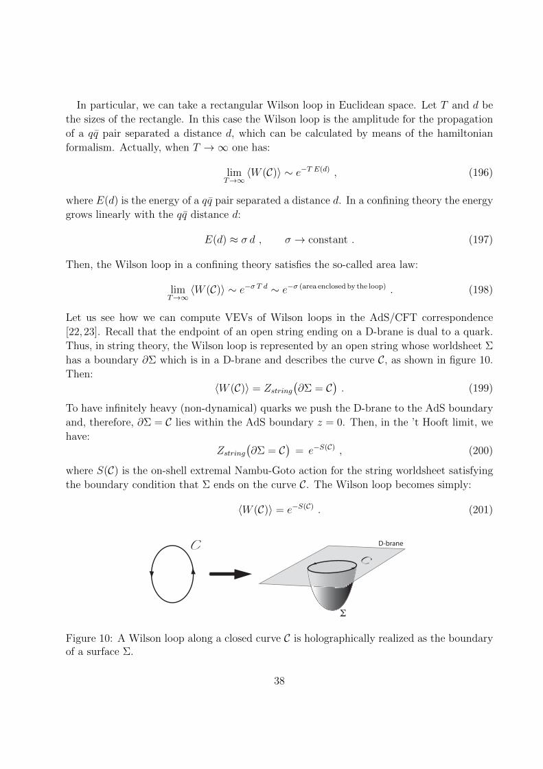
In particular, we can take a rectangular Wilson loop in Euclidean space. Let T and d be

the sizes of the rectangle. In this case the Wilson loop is the amplitude for the propagation

of a qq pair separated a distance d, which can be calculated by means of the hamiltonian

formalism. Actually, when T →∞ one has:

limT→∞

〈W (C)〉 ∼ e−T E(d) , (196)

where E(d) is the energy of a qq pair separated a distance d. In a confining theory the energy

grows linearly with the qq distance d:

E(d) ≈ σ d , σ → constant . (197)

Then, the Wilson loop in a confining theory satisfies the so-called area law:

limT→∞

〈W (C)〉 ∼ e−σ T d ∼ e−σ (area enclosed by the loop) . (198)

Let us see how we can compute VEVs of Wilson loops in the AdS/CFT correspondence

[22, 23]. Recall that the endpoint of an open string ending on a D-brane is dual to a quark.

Thus, in string theory, the Wilson loop is represented by an open string whose worldsheet Σ

has a boundary ∂Σ which is in a D-brane and describes the curve C, as shown in figure 10.

Then:

〈W (C)〉 = Zstring(∂Σ = C

). (199)

To have infinitely heavy (non-dynamical) quarks we push the D-brane to the AdS boundary

and, therefore, ∂Σ = C lies within the AdS boundary z = 0. Then, in the ’t Hooft limit, we

have:

Zstring(∂Σ = C

)= e−S(C) , (200)

where S(C) is the on-shell extremal Nambu-Goto action for the string worldsheet satisfying

the boundary condition that Σ ends on the curve C. The Wilson loop becomes simply:

〈W (C)〉 = e−S(C) . (201)

C C D-brane

!

Figure 10: A Wilson loop along a closed curve C is holographically realized as the boundaryof a surface Σ.

38

We will now apply these ideas to the holographic calculation of the rectangular Wilson

loop and the corresponding qq potential energy in N = 4 SYM. With this purpose, let us

consider a string ending on the boundary of AdS5, where it extends along one of the gauge

theory coordinates (say x1 ≡ x). We shall parameterize the embedding of the string in AdS5

by a function z = z(x) and we will denote by z′ the derivative of z with respect to x. The

induced metric in Euclidean signature on the string worldsheet is:

ds2 =L2

z2

[dt2 + (1 + z′ 2) dx2

]. (202)

Therefore, the Nambu-Goto action for the string is:

S =1

2πα′

∫dt

∫dx√g =

TL2

2πα′

∫dx

√1 + z′ 2

z2, (203)

where T =∫dt. The action (203) corresponds to a problem in classical mechanics where x

is the “time” and the lagrangian is given by:

L =TL2

2πα′

√1 + z′ 2

z2. (204)

Since this lagrangian does not depend on the “time” x , the “energy” is conserved, which

means that:

z′∂L∂z′− L = constant . (205)

By computing the derivative of L appearing on the left-hand side of (205), the conservation

law written above can be proved to be equivalent to the following first integral of the equation

of motion:

z2√

1 + z′ 2 = constant . (206)

For the hanging string configuration we are interested in, the boundary conditions that the

function z(x) must satisfy are:

z(x = −d/2

)= z(x = d/2

)= 0 , (207)

where d is the quark-antiquark separation. Clearly, there is a value of x for which z is

maximal. By symmetry this value is just x = 0 and, since z(x) has a maximum implies that

z′(x = 0) = 0. Let z∗ be the maximal value of z, i.e. z∗ = z(x = 0). Then, the constant

appearing in the conservation law is just z2∗ and we have:

z′ = ±√z4∗ − z4

z2, (208)

where the two signs correspond to the two sides of the hanging string. The equation written

above can be integrated immediately to give x as a function of z:

x = ±∫ z

z∗

ξ2√z4∗ − ξ4

dξ . (209)

39

By introducing a new rescaled variable y by means of the relation ξ = z∗y, one can write:

x = ±z∗∫ z

z∗

1

y2√1− y4

dy . (210)

By imposing the boundary conditions (207), we can obtain the quark-antiquark separation

as a function of z∗:d

2= z∗

∫ 1

0

y2√1− y4

dy . (211)

The integral over y in (211) can be computed exactly and one gets:

z∗ =d

2√

2 π32

(Γ(1

4

))2

. (212)

Then, it follows that d and z∗ are proportional. Let us now compute the on-shell action

for the string, from which we will obtain the quark-antiquark potential. By plugging the

conservation law (206) inside the expression of the action in (203), we get:

S =T L2z2

∗2πα′

∫dx

z4. (213)

Let us change variables in the integral (213) from x to z. The jacobian for this change of

variables is:dx

dz=

1

z′=

z2√z4∗ − z4

, (214)

where we have taken into account the value of z′ written in (208). Taking into account that

the variable z is double-valued, the total action is:

S = 2× TL2z2∗

2πα′

∫ z∗

ε

dz

z2√z4∗ − z4

. (215)

Let us next work on a rescaled variable y, related to z as z = z∗y. Then, the on-shell action

becomes:

S =TL2

πα′z∗Iε , (216)

where Iε is the following integral:

Iε =

∫ 1

ε/z∗

dy

y2√

1− y4. (217)

The integral Iε in (217) diverges when ε→ 0. Indeed, one can prove that, for small ε:

Iε = − π32

√2(

Γ(

14

))2 +z∗ε. (218)

40

The on-shell action S is just T E, where E is the energy of the quark-antiquark. It follows

that E is given by:

E = − 4π2L2(Γ(

14

))4

α′

1

d+

L2

πα′1

ε. (219)

The divergent term in (219) corresponds to the quark and antiquark masses (which are

considered to be infinitely large in the static limit). To check this, let us compute the

euclidean action of a single string which goes straight from the boundary z = ε to z =∞ at

fixed x. This configuration can be described by using t and z as worldvolume coordinates.

The induced metric is obtained by keeping constant the x coordinate and is given by:

ds2 =L2

z2(dt2 + dz2) . (220)

The on-shell Nambu-Goto action for this configuration is:

S| =T

2πα′

∫ ∞ε

L2

z2dz2 =

TL2

2πα′ ε. (221)

Therefore, the energy for a configuration of two straight parallel strings in AdS5 is:

E| | = 2× L2

2πα′ ε, (222)

which is equal to the divergent term in (219), as claimed. The quark-antiquark potential Vqqis obtained by subtracting the divergent contribution due to the quark masses:

Vqq = E − E| | . (223)

By subtracting (219) and (222), one gets:

Vqq = − 4π2L2(Γ(

14

))4

α′

1

d. (224)

Let us write this result in terms of gauge theory quantities. Recall that L2 =√N2gYM α′

or, equivalently L2 =√λα′. Then, (224) can be rewritten as:

Vqq = − 4π2√λ(

Γ(

14

))4

1

d. (225)

The Coulombic 1/d dependence in (225) is consequence of the conformal invariance of the

theory. The non-analytic dependence on the coupling λ is a non-perturbative effect. In field

theory this non-analyticity results from the summation of an infinite number of Feynman

41

diagrams. It is interesting to compare (225) with the perturbative qq potential, valid for

small λ, which is given by:

Vqq = −πλd. (226)

Remarkably we have been able to find a non-perturbative result in a interacting quantum

field theory by studying the catenary curve for a hanging string in classical gravity.

In the next two sections we will generalize the result (225) to the case of N = 4 SYM at

finite temperature and to the gravity dual of a theory in which the quarks are confined. In

the former case we have to study a string hanging from the boundary of an anti-de-Sitter

black hole, whereas in the latter we must deal with a geometry obtained from the AdS black

hole by a double analytic continuation.

10.1 Quark-antiquark potential at finite temperature

Let us suppose that we put our gauge theory in a thermal bath at a temperature T . In the

holographic correspondence the heat bath is dual to a bulk geometry with an event horizon

(a black hole) and the Hawking temperature of the black hole is identified as the temperature

of heat bath. In particular, the dual of N = 4 SYM at finite temperature is a black hole in

AdS5, whose metric in euclidean space is (see below):

ds2 =L2

z2

[f(z) dt2 + d~x 2 +

dz2

f(z)

], (227)

with f(z) being the following function:

f(z) = 1 − z4

z40

. (228)

The parameter z0 corresponds to the position of the horizon and is related to the black hole

temperature T as T = (πz0)−1 (see section 11.2 below). In the context of the holographic

duality one naturally identifies the black hole temperature T with the temperature of the

gauge theory.

As in the zero temperature case, we will parametrize the embedding of the string by a

function z = z(x). The induced metric is:

ds2 =L2

z2

[f dt2 +

(1 +

z′ 2

f

)dx2

]. (229)

The Nambu-Goto action for this embedding becomes:

S =τL2

2πα′

∫dx

√f(z) + z′ 2

z2, (230)

42

where τ =∫dt. Following the same steps as in the zero temperature case, it is straightfor-

ward to derive the following first integral of the equation of motion:

z2√f(z) + z′ 2

f(z)= constant =

z2∗√f(z∗)

. (231)

From (231) we obtain readily the value of z′:

z′ = ±

√f(z)

f(z∗)

√z4∗ − z4

z2. (232)

Let us now define the constant ρ as follows:

ρ ≡(z0

z∗

)4

. (233)

Then, we have:

x = ±z∗√ρ− 1

∫ zz∗

1

y2dy√(1− y4)(ρ− y4)

, (234)

and the quark-antiquark distance d is equal to:

d = 2z∗√ρ− 1

∫ 1

0

y2dy√(1− y4)(ρ− y4)

. (235)

Notice that these expressions become the ones at zero temperature as ρ→∞, as it should.

Moreover, as z∗ → z0, ρ→ 1 and the distance d→ 0 (see figure 11). Actually, by varying ρ

one can see that there is a maximal value of d (dmax ∼ z0) and the qq bound state becomes

unbound due to thermal screening, in agreement with the behavior expected from the point

of view of the gauge theory at non-zero temperature.

10.2 Quark-antiquark potential in a confining background

Let us consider the AdS black hole in Euclidean signature and let us go back to Minkowski

signature by analytic continuation along a different direction, namely by making x3 → it. If

we call u to the original euclidean time, we arrive at the following metric:

ds2 =L2

z2

[− dt2 + dx 2

1 + dx 22 + f(z)du2 +

dz2

f(z)

]. (236)

In this case the space ends smoothly at z = z0, which should be though as a IR mass scale. We

will now compute the qq potential for the metric (236) and we will verify that it corresponds

to a confining background. With this purpose, let us consider a fundamental string in the

43

Horizon

L

ds2 =L2

z2

!

f(z) dt2 + d!x 2 +dz2

f(z)

"

f(z) = 1 !

z4

z40

T =1

!z0

Consider an AdS black hole

Quark-antiquark potential at finite temperature

S =!L2

2"#!

!

dx

"

f(z) + z! 2

z2! =

!dtAction

z2!

f(z) + z! 2

f(z)= constant =

z2"

!

f(z")First integral

Ls

Horizonz = z0

Temperature

2 4 6 8 10

0.2

0.4

0.6

0.8

! !

!

z0

z!

"4

d = 2z!!

! ! 1

" 1

0

y2dy!

(1 ! y4)(! ! y4)qq distance

d

z!

!

z! ! z0 ! ! 1 d ! 0

There is a maximal value of d (dmax ! z0)

Models thermal screening in a plasma!

At high T ! disconnected configuration energetically favored

Figure 11: In a black hole metric, the string ends on the horizon when the qq separation islarge enough. Correspondingly, the distance d reaches a maximum value, as the plot on theright shows.

euclidean version of the above metric and let us use (t, x) as worldsheet coordinates. The

induced metric is:

ds2 =L2

z2

[dt2 +

(1 +

z′ 2

f

)dx2

], (237)

and the Nambu-Goto action becomes:

S =τL2

2πα′

∫dx

z2

√1 +

z′ 2

f(z), (238)

where τ =∫dt. The first integral corresponding to the action (238) is:

z2√f(z)

√f(z) + z′ 2 = z2

∗ , (239)

from which we get:

z′ = ±√f(z)

√z4∗ − z4

z2. (240)

This equation can be integrated as:

x = ±z∗√ρ

∫ zz∗

1

y2dy√(1− y4)(ρ− y4)

, (241)

where the constant ρ is the same as in (233). It follows that the qq distance d is:

d = 2z∗√ρ

∫ 1

0

y2dy√(1− y4)(ρ− y4)

. (242)

44

In this case, d grows without limit as ρ→ 1, or equivalently as the turning point approaches

the end of the space (i.e. when z∗ → z0) (see figure 12). In the large d limit the profile of

the hanging string is approximately rectangular. The energy due to the vertical parts of the

profile can be identified with the masses of the static quarks, which have to be subtracted

to get the potential energy. The qq potential is just due to the horizontal part of the profile.

Since in this part z is approximately constant and equal to z0, we get that the contribution

to the euclidean action is:

Shorizontal =τL2

2πα′d

z20

, (243)

which corresponds to an area law (it is proportional to τd) and gives rise to a confining

potential of the type:

V = σs d , (244)

with σs being the effective string tension, given by:

σs =L2

2πα′1

z20

. (245)

In terms of gauge theory quantities, σs can be written as:

σs =

√λ

2πz20

. (246)

Notice that M ∼ 1/z0 is an IR scale that can be identified with the mass gap of the theory

(and z0 with the glueball size). The previous formula for the tension is simply:

σs ∼√λM2 . (247)

11 Black hole thermodynamics

The partition function in statistical mechanics in the canonical ensemble is given by:

Z = Tr e−HT , (248)

where, H is the hamiltonian operator, T is the temperature and we are taking the Boltzmann

constant kB = 1. The thermal average of an operator O at the temperature T is:

〈O〉T =Tr[O e−HT

]Z

. (249)

In the path integral approach, the average 〈O〉T can be written as:

〈O〉T ∼∫

[Dψ] 〈ψ(x), t |O e−HT |ψ(x), t〉 , (250)

45

Z=0

Z=Z0

1.1 1.2 1.3 1.4 1.5

1.5

2.0

2.5

3.0

d = 2z!!

!

! 1

0

y2dy"

(1 " y4)(! " y4)! !

!

z0

z!

"4

d

z!

!

No maximal distance

The distance diverges as we approach the end of the space

z = z0

z = 0.

V = !s d !s =L2

2"#!

1

z20

!s =

!

"

2#z20

M !

1

z0

z0 ! glueball size

!s !

"

" M2

Qualitative picture

When d ! " the profile is almost rectangular

Horizontal part ! qq potential

Vertical parts ! masses of the static quarks

Shorizontal =!L2

2"#!

d

z20

Area law Confinement

mass gap

effective string tension

Figure 12: In a confining metric the space ends smoothly and the profile of the hanging stringbecomes almost rectangular for large qq separation (left). The distance d is not bounded, asshown on the plot on the right.

where the expectation value is taken between the same initial and final state |ψ(x), t〉 (as

it corresponds to a trace in Hilbert space). Equivalently, since the hamiltonian operator

implements time evolution, we can rewrite (250) as:

〈O〉T ∼∫

[Dψ] 〈ψ(x), t |O|ψ(x), t+i

T〉 . (251)

Then, to perform thermal averages we have to consider imaginary time evolution and we

have to impose periodic boundary conditions in the Hilbert space (antiperiodic for fermions).

Then, the euclidean time tE must be periodically identified

tE ≡ tE +1

T. (252)

Thus, the compactification of Euclidean time is equivalent to having T 6= 0.

Let us apply these ideas to obtain the Hawking temperature of a black hole. We will

assume that we have an euclidean metric of the type:

ds2 = g(r)[f(r) dt2E + d~x 2

]+

1

h(r)dr2 , (253)

where the functions f(r) and h(r) have a first-order zero at r = r0, which is the location of

the horizon, and g(r0) 6= 0. Then, for r ≈ r0

f(r) ≈ f ′(r0) (r − r0) , h(r) ≈ h′(r0) (r − r0) , (254)

while we can take g(r) = g(r0). Then, the near-horizon euclidean metric can be written as:

ds2 ≈ g(r0)[f ′(r0) (r − r0)dt2E + d~x 2

]+

1

h′(r0)

dr2

r − r0

. (255)

46

Let us define a new radial variable ρ such that:

1

h′(r0)

dr2

r − r0

= dρ2 , (256)

which can be integrated to give the following relation between ρ and r:

ρ = 2

√r − r0

h′(r0). (257)

Next, we define an angular coordinate θ such that

g(r0) f ′(r0) (r − r0)dt2E = ρ2 dθ2 , (258)

which is equivalent to defining θ as:

θ =1

2

√g(r0) f ′(r0)h′(r0) tE . (259)

In the new variables, the (tE, r) part of the metric takes the form dρ2 +ρ2dθ2, which is locally

like the flat metric of a plane. In order to have ρ = 0 (i.e. the horizon) as a regular point

without any curvature singularity, the variable θ must be a periodic variable with period

2π. Otherwise we would have a conical singularity at the origin, due to the defect angle.

We have argued above for a general system that the compactification of the euclidean time

is equivalent to having a non-zero temperature T . Thus, it follows that we can assign a

temperature T to a black hole (the Hawking temperature). In order to find the value of

T , let us notice that the periodicity under θ → θ + 2π is equivalent to periodicity under

tE → tE + 1T

, where T is the Hawking temperature given by:

1

T=

4π√g(r0) f ′(r0)h′(r0)

. (260)

In the next subsections we will apply this formula to determine the Hawking temperature of

a couple of black holes.

11.1 Application to the Schwarzschild black hole

Let us consider the ordinary Schwarzschild metric in four dimensions:

ds2 = −(

1− 2GM

r

)dt2 +

dr2

1− 2GMr

+ r2dΩ22 , (261)

which is a particular case of the general expression written in (253), with the functions f , h

and g being given by:

g(r) = 1 , f(r) = h(r) = 1− 2GM

r. (262)

47

In (261) G is the four-dimensional Newton constant and M is the mass of the black hole.

The horizon in the geometry (261) is located at r = r0 = 2GM . Since:

f ′(r0) = h′(r0) =2GM

r20

(263)

it follows that the Hawking temperature for the Schwarzschild black hole is given by:

T =1

8πGM. (264)

Let us use the expression of T in (264) to obtain the black hole entropy S of the Schwarzschild

black hole. We will identify the mass M with the internal energy and we will make use of

the first law of thermodynamics:

dM = TdS =1

8πGMdS , (265)

which can be integrated to give the entropy S:

S = 4π GM2 , (266)

The horizon area AH for the metric (261) is the area of the surface t = constant, r = r0. It

is straightforward to demonstrate that AH is:

AH = 4πr20 = 16G2M2 . (267)

It is now immediate to check that the relation between S and AH is:

S =AH4G

, (268)

which is noting but the celebrated Bekenstein-Hawking entropy formula which relates the

entropy of a black hole with the area of its horizon (see (6)).

11.2 AdS black hole

The metric of a black hole in AdSd+1 is:

ds2 =L2

z2

[f(z) dt2E + d~x 2 +

dz2

f(z)

], (269)

where f(z) is the following function:

f(z) = 1 − zd

zd0, (270)

48

with z0 being a constant (z = z0 is the location of the horizon). This metric is just of our

general form (253) with r → z, f given as above and g and h being:

g =L2

z2, h =

z2

L2f . (271)

In this case the derivatives of f and h at the horizon are:

f ′(z0) = − d

z0

, h′(z0) = −dz0

L2, (272)

and, therefore, we have:

g(z0) f ′(z0)h′(z0) =d2

z20

. (273)

Thus, the Hawking temperature is related to z0 by means of the relation:

T =d

4πz0

. (274)

The horizon is the hypersurface z = z0 and t constant, whose area in the metric (269) is:

AH =(Lz0

)d−1

Vd−1 , (275)

where Vd−1 is the volume along the Minkowski spacial directions. In terms of the temperature,

AH can be written as:

AH =(4π

d

)d−1

Ld−1 T d−1 Vd−1 , (276)

and the entropy can be computed from the Bekenstein-Hawking formula, with the result:

S =AH

4Gd+1

=1

4Gd+1

(4π

d

)d−1

Ld−1 T d−1 Vd−1 . (277)

We now define the entropy density s as:

s =S

Vd−1

. (278)

Let us write s in terms of the QFT central charge cQFT = 14(L/lP )d−1. We get:

s =(4π

d

)d−1

cQFT Td−1 . (279)

In the case of N = 4 SYM, we take d = 4 and cSYM = N2/2π and the entropy density is

given by:

sSYM =π2

2N2 T 3 . (280)

49

From the expression of the entropy density in (280) we can obtain the value of the pressure

by means of the thermodynamic relation:

s =∂p

∂T. (281)

We get:

p =π2

8N2 T 4 . (282)

Moreover, the energy density ε can be obtained from p and s by means of the standard

thermodynamic relation:

ε = −p+ Ts . (283)

Using the values of p and s computed from holography, we arrive at the following value of

the energy density:

ε =3π2

8N2 T 4 . (284)

11.3 Comparison with field theory

Let us compare the strong coupling values of s, p and ε found above with those corresponding

the N = 4 SYM at zero coupling. The partition function in the canonical ensemble for a

gas of non-interacting relativistic bosons and fermions is

logZ = ∓V3

∫d3p

(2π)3log(

1∓ e−ω(p)T

), (285)

where the upper minus (lower plus) signs corresponds to bosons (respectively, fermions) and

ω(p) =√~p 2 +m2. In the massless case, we just take ω(p) = |~p| and we get:

logZ

V3

= ∓∫ ∞

0

dp

2π2p2 log

(1∓ e−

pT

). (286)

Let us change variables in the integral (286) from p to x = p/T . After integrating by parts

we find:logZ

V3

=T 3

6π2

∫ ∞0

dxx3

ex ∓ 1. (287)

To calculate these integrals we use the general results, valid for n ∈ Z:∫ ∞0

dxx2n−1

ex + 1=

22n−1 − 1

2nπ2nBn ,

∫ ∞0

dxx2n−1

ex − 1=

(2π)2nBn

4n, (288)

where Bn denotes the Bernouilli numbers. In particular for n = 2, since B2 = 1/30, we

have: ∫ ∞0

dxx3

ex − 1=

π4

15,

∫ ∞0

dxx3

ex + 1=

7π4

120. (289)

50

Thus, for bosons:logZ

V3

=π2

90T 3 , (bosons) , (290)

while for fermions:logZ

V3

=7π2

720T 3 , (fermions) . (291)

The entropy density can be obtained from the partition function by means of the standard

statistical mechanics relation:

s =∂

∂T

[T

logZ

V3

]= 4

logZ

V3

. (292)

Then, it follows that:

sboson =2π2

45T 3 , sfermion =

7π2

180T 3 . (293)

In N = 4 SYM the number of bosons we have is:[2(gauge field) + 6(scalar field)

]N2 = 8N2 , (294)

while the number of fermions is:[2× 4(Weyl spinors)

]N2 = 8N2 , (295)

which, due to the supersymmetry, is the same as the number of bosons. Therefore, the total

entropy density of N = 4 SYM when the coupling constant is zero is:

sN=4 free gas = 8N2[2π2

45+

7π2

180

]T 3 =

2π2

3N2 T 3 . (296)

By using the thermodynamic formulas (283) and (281), we obtain the values of the pressure

and energy density:

pN=4 free gas =π2

6N2 T 4 , εN=4 free gas =

π2

2N2 T 4 . (297)

Then, by comparing with the result given by the black hole, we obtain:

sblack hole =3

4sN=4 free gas , (298)

and similarly for the pressure and energy density:

pblack hole =3

4pN=4 free gas , εblack hole =

3

4εN=4 free gas . (299)

Therefore, the AdS/CFT correspondence predicts that the values of s, p and ε at infinite

coupling differ from their values at zero coupling by a multiplicative factor 3/4. These

reductions of the entropy, pressure and energy density as the coupling is increased are in

very good agreement with the results obtained in lattice simulations for different gauge

theories.

51

12 Transport coefficients

Let us begin by writing the linear response formulas of section 9.2 in real time. We consider

a system in QFT to which we couple a source ϕ(x) to a local operator O(x):

S = S0 +

∫ddxO(x)ϕ(x) , (300)

where the d-dimensional spacetime has Minkowski signature. We will assume that the un-

perturbed VEV of the operator O vanishes. Then, the one-point function of the operator Oin the presence of the source is given by:

〈O(x)〉ϕ = −∫GR(x− y)ϕ(y) dy , (301)

where GR(x− y) is the retarded Green’s function, defined as:

i GR(x− y) ≡ θ(x0 − y0) 〈[O(x),O(y)

]〉 . (302)

The fact that the linear response is determined by the retarded correlator is a consequence

of causality since the source can influence the system only after it has been turned on. In

momentum space the relation (301) between the one-point function and the source becomes:

〈O(ω,~k)〉ϕ = −GR(ω,~k )ϕ(ω,~k ) . (303)

We are interested in analyzing the long wavelength hydrodynamic limit. In this case one

can take the zero spatial momentum and zero frequency limit of the retarded correlator. In

this limit one studies the response of the system to a time varying source ϕ(t), which can be

approximately represented as:

〈O〉ϕ ≈ −χ ∂t ϕ , (304)

where the real constant χ is the so-called transport coefficient. In frequency space, for ω → 0,

the relation (304) is given by:

〈O〉ϕ ≈ i ω χϕ(ω) . (305)

The linear response equation for this quantity is obtained from the long wavelength limit~k → 0 of (303):

〈O〉ϕ = −GR(ω,~k = 0 )ϕ(ω) . (306)

By comparing (305) and (306) we get:

GR(ω,~k = 0) = −iω χ , (ω → 0) , (307)

or, taking the imaginary part:

ImGR(ω,~k = 0) = −ω χ , (ω → 0) . (308)

52

From (308) we immediately get the so-called Kubo formula for χ:

χ = − limω→0

lim~k→0

1

ωImGR(ω,~k) . (309)

Let us now see how we can make use of (309) to compute the transport coefficient χ by

using holographic methods. Let us consider a (d+ 1)-dimensional metric of the form:

ds2 = gtt dt2 + gzzdz

2 + gxxδij dxidxj . (310)

We will assume the metric (310) has an horizon at z = z0 and that gtt and that gzz behave

near z = z0 as:

gtt ≈ −c0(z0 − z) , gzz ≈cz

z0 − z, z → z0 , (311)

with c0 and cz being constants. Let us consider a massless scalar field φ in this metric such

that its action is:

S = −1

2

∫dd+1 x

√−g ∂M φ ∂M φ

q(z), (312)

where the function q(z) is an effective coupling of the mode. The Euler-Lagrange equation

of motion derived from (312) is:

∂M

(√−gq

gMN ∂M φ)

= 0 . (313)

In terms of the canonical momentum Π, defined as (see (141)):

Π ≡ − ∂L∂(∂zφ)

=

√−gq

gzz ∂z φ , (314)

the equation of motion (313) becomes:

∂z Π = −√−gq

( ∂2t φ

gtt+∂2i φ

gxx

). (315)

Let us now Fourier transform φ and Π in the variables t, ~x:

φ(z, t, ~x) =

∫dω dd−1k

(2π)dei(

~k·x−ωt) φ(z, ω,~k) ,

Π(z, t, ~x) =

∫dω dd−1k

(2π)dei(

~k·x−ωt) Π(z, ω,~k) . (316)

Since in this massless case the scaling dimension ∆ is equal to d (see (112) for m = 0), the

one-point function is just the limit of the momentum Π at the boundary z = 0 and the

53

boundary field ϕ is just obtained by taking the limit z → 0 of the bulk field φ, without any

multiplicative factor (see eqs. (147) and (129)). It follows from (305) that the transport

coefficient χ is obtained as:

χ = limkµ→0

limz→0

Im

[Π(z, kµ)

ω φ(z, kµ)

]= lim

kµ→0limz→0

Π(z, kµ)

iω φ(z, kµ), (317)

where, in the last step, we used the fact that ReΠ/ω → 0 as ω → 0 (see below). It turns

out that evaluating Π/(ω φ) at the boundary is equivalent to evaluate it at the horizon. In

order to prove this, let us consider the general equation:

∂z[A(z) ∂zφ

]= B(z)φ(z) . (318)

Let us write (318) in hamiltonian form. We first define:

P (z) ≡ A(z) ∂zφ(z) . (319)

Then, (318) can be written as:

∂z P (z) = B(z)φ(z) . (320)

Then, one can readily prove that (318) and (320) can be combined in the following first-order

Riccati equation:

∂z

(P (z)

φ(z)

)= B(z) − 1

A(z)

(P (z)

φ(z)

)2

. (321)

For the equation of motion of the scalar field φ in momentum space, the functions A(z) and

B(z) are given by:

A(z) =

√−gq

gzz , B(z) =

√−gq

[ω2

gtt+

~k 2

gxx

], (322)

and P (z) = Π(z) (see (314)). Then, we can write:

∂z

[Π

ωφ

]= −ω

[qgzz√−g

(Π

ωφ

)2

−√−gq gtt

(1 +

gttgxx

~k 2

ω2

)]. (323)

The right-hand side of equation (323) vanishes when the ordered limit limω→0 lim~k→0 is

taken. It follows that Π/(ωφ) is independent of z in this limit and, as claimed above, it can

be evaluated at the horizon. Thus, we can write the transport coefficient χ as:

χ = limkµ→0

limz→z0

Π(z, kµ)

iω φ(z, kµ). (324)

54

In order to evaluate the right-hand side of (324), let us study the equation of motion near

z = z0, where Π becomes:

Π ≈ 1

cz

√−g(z0)

q(z0)(z0 − z) ∂z φ , (325)

and the equation of motion takes the form:

∂z

[(z0 − z) ∂z φ(z, kµ)

]+ cz

[ ω2

c0(z0 − z)− k2

gxx(z0)

]φ(z, kµ) = 0 . (326)

To find an approximate solution of (326) near the horizon z = z0, we neglect the last term

in the previous equation and try to find a solution of the type:

φ = (z0 − z)β . (327)

Plugging the ansatz (327) in (326), we get that the exponent β can take the following two

values:

β = ±i√czc0

ω , (328)

which correspond to the following two solutions:

φ± ∼ (z0 − z)±i√

czc0

ω. (329)

Only one of the two solutions in (329) is compatible with causality. Indeed, let us define

a new variable r as z0 − z = er. In the r variable the horizon is located at r → −∞. By

inserting the t dependence, the two solutions φ± are:

φ± ∼ e−i(ω t∓Ω r) , (330)

where Ω = ω√cz/c0. Clearly, φ− is an incoming wave at the horizon since if we increase

t→ t+ε, we must decrease r as r → r−εΩ/ω to keep φ− constant. Then, the wave φ− moves

towards the horizon r → −∞ and is an infalling wave at the horizon. Similarly, φ+ is an

outgoing wave at the horizon. Causality on the gravity side, is implemented if we choose our

solution to be the infalling one φ−. One can show that this corresponds to having retarded

Green’s functions on the field theory side. This infalling solution near z = z0 satisfies:

∂zφ− =

√gzz(z0)

−gtt(z0)iω φ− , (331)

and, therefore, one has:

Π

iω φ−

∣∣∣∣∣z0

=1

q(z0)

√g

gzz gtt

∣∣∣∣∣z0

. (332)

55

It follows that the transport coefficient χ is given by:

χ =1

q(z0)

√g

gzz gtt

∣∣∣∣∣z0

. (333)

Notice that the square root in this last equation is just the area of the horizon AH divided

by the spatial volume V . Then, we can alternatively write the transport coefficient χ as:

χ =1

q(z0)

AHV

. (334)

In particular, for an AdS black hole, the previous expression becomes:

χ =1

q(z0)

(Lz0

)d−1

, (AdS black hole) . (335)

More interestingly, one can compare the general formula (334) with the entropy density, as

given by the Bekenstein-Hawking formula s = AH/(4GNV ). By computing the ratio χ/s,

we get the simple result:χ

s=

4GN

q(z0). (336)

13 Holographic viscosities

Hydrodynamics can be thought as an effective theory describing the dynamics of a continuous

system at large distances and time scales. In order to study the dynamics of the system we

have to analyze the energy-momentum tensor T µν which is conserved (∂µTµν = 0). We will

assume that the system is at local thermal equilibrium and that the state of the system at

a given time is determined by the local temperature T (x) and the local fluid velocity uµ(x),

which satisfies the condition uµuµ = −1.

The relation between T µν and uµ and the thermodynamic functions is expressed by means

of the so-called constitutive relations, which for isotropic fluids takes the form:

T µν = (ε+ p)uµuν + p gµν − σµν , (337)

where ε is the energy density and p is the pressure, while σµν is the so-called dissipative

part of T µν and depends on the derivatives of T (x) and uµ. In order to parametrize σµνat first-order in the derivatives, let us consider a local rest frame in which ui(x) = 0 (and

uµ = (1, 0, 0, 0)). One can choose this frame in such a way that the dissipative corrections to

the energy-momentum tensor components T 0µ vanish. Then, σ00 = σ0i = 0 or, equivalently,

T 00 = ε, T 0i = 0. The only non-zero elements of the dissipative energy-momentum tensor

are σij. At first order in derivatives σij can be written as:

σij = η(∂iuj + ∂jui −

2

3δij ∂kuk

)+ ζ δij∂kuk , (338)

56

where η is the so-called shear viscosity and ζ is the bulk viscosity.

Let us write σµν in covariant form. We first define the projector onto the directions

perpendicular to uµ, as:

P µν = gµν + uµuν . (339)

Then, in an arbitrary curved metric σµν can be written as:

σµν = P µα P νβ[η(∇αuβ +∇βuα

)+(ζ − 2

3η)gαβ∇ · u

], (340)

where the covariant derivatives of the vectors uβ are defined as:

∇αuβ = ∂αuβ − Γµαβ uµ , (341)

with Γµαβ being the Christoffel symbols, defined as:

Γµαβ =1

2gµλ[ ∂gλα∂xβ

+∂gλβ∂xα

− ∂gαβ∂xλ

]. (342)

We will find σµν as (minus) the one-point function of T µν in the presence of a metric per-

turbation of the type gµν → ηµν + hµν . By using linear response theory (eq. (301)), we

obtain:

σµν(x) =

∫Gµν,αβR (x− y)hαβ(y)dy , (343)

where the retarded correlator is just:

i Gµν,αβR (x− y) = θ(x0 − y0) 〈

[T µν(x), Tαβ(y)

]〉 . (344)

Let us now consider the following metric perturbation:

g00(t, ~x) = −1 , g0i(t, ~x) = 0 , gij(t, ~x) = δij + hij(t) . (345)

with hij << 1 and such that is traceless (hii = 0). We will assume that hij is a function of t

and that this variation with t is slow. The inverse metric is just:

g00(t, ~x) = −1 , g0i(t, ~x) = 0 , gij(t, ~x) = δij − hij(t) , (346)

from which we get the different components of the projector P µ ν :

P 00 = 0 , P 0i = 0 , P ij = δij − hij . (347)

At first order in the perturbation, the Christoffel symbols are given by:

Γ000 = Γ0

0i = 0 , Γ0ij =

1

2∂0 hij . (348)

57

Therefore the covariant derivatives of the velocity are:

∇0u0 = ∇0ui = 0 , ∇iuj =1

2∂0 hij . (349)

From these values and the hypothesis that the metric perturbation is traceless it follows that

the covariant divergence of the velocity vanishes:

∇ · u =1

2∂0 hii = 0 . (350)

Let us assume that the only non-zero value of hij is h12. Then, the linear response value of

σ12 in frequency space is:

σ12(ω) = G12,12R (ω,~k = 0)h12(ω) . (351)

Moreover, by using the values of the covariant derivatives of the velocity we get

σ12(t) = η ∂0h12(t) , (352)

or, in frequency space (for low ω):

σ12(ω) = −iη ω h12(ω) . (353)

By comparing these two expressions of σ12, we obtain again Kubo formula for the shear

viscosity, namely:

η = − limω→0

[ 1

ωImG12,12

R (ω,~k = 0)]. (354)

In order to compute holographically the retarded correlator of T12, let us consider a general

d + 1-dimensional diagonal metric and let us perturb it by adding a non-diagonal element

along x1 x2:

ds2 = gtt dt2 + gzzdz

2 + gxx(δij dx

idxj + 2φ dx1dx2), (355)

where φ is small and independent of x1 and x2. Notice that, in the perturbed metric at first

order in φ, one has:

g12 = gxx φ , g12 = φ . (356)

Let us write the x1x2 part of the metric (at first order) as:

gxx(dx1)2 + gxx(dx

2 + φ dx1)2 , (357)

which is clearly similar to the ansatz corresponding to a Kaluza-Klein reduction along x2

with KK gauge field connection:

A = φ dx1 . (358)

58

Therefore, we can use the known results of the KK reduction to write the quadratic action

for φ. Indeed, the Einstein-Hilbert action for the metric leads to the following expression for

the action of the gauge connection A (or equivalently the metric perturbation φ):

Sφ = − 1

16πGN

∫dd+1x

√−g gxx

F 2

4, (359)

where g is the determinant of the unperturbed metric (with φ = 0), F = dA is the field

strength of A and in F 2 = Fµν Fµν the indices are raised with the unperturbed metric. As:

F = ∂tφ dt ∧ dx1 + ∂3φ dx3 ∧ dx1 + ∂zφ dz ∧ dx1 , (360)

we have:

F 2 =2

gxx

[gtt (∂t φ)2 + gxx (∂3 φ)2 + gzz (∂z φ)2

], (361)

or, taking into account that ∂1 φ = ∂2 φ = 0:

F 2 =2

gxxgMN ∂M φ ∂N φ . (362)

Thus, the action for the perturbation φ is:

Sφ = − 1

16πGN

∫dd+1x

√−g 1

2gMN ∂M φ ∂N φ , (363)

which is the canonical form of the action for a scalar field, with normalization constant

q = 16π GN . (364)

It follows from our general calculation of section 12 of the transport coefficients for a scalar

field that the shear viscosity is given by:

η =1

16π GN

AHV

, (365)

and, therefore, the ratio η/s is just [24,25]:

η

s=

1

4π. (366)

In ordinary units the ratio η/s is given by:

η

s=

~4πkB

, (367)

where kB is the Boltzmann constant. Notice that this result does not depend on the metric

chosen. It is valid for any theory with a gravity dual given by Einstein gravity coupled to

59

matter fields. In this sense it is a universal result valid at λ → ∞ (infinite coupling limit).

The finite coupling corrections can also be calculated. For N = 4 SYM one gets:

η

s=

1

4π

(1 +

15 ζ(3)

λ32

+ · · ·), (368)

where ζ(x) is the Riemann zeta function (ζ(3) = 1.2020). In general, η/s at λ→∞ is very

small:η

s= 0.07957 . (369)

The finite coupling corrections make η/s increase. It is interesting to compare with the weak

coupling calculation, valid when λ→ 0:

η

s=

A

λ2 log(B√λ

) , (370)

where A and B are constant coefficients that depend on the theory. Notice that in (370)

η/s → ∞ as λ → 0. This is because a weakly coupled gauge theory is a gas with strong

dissipative effects, in which momentum can be transported over long distances due to the

long free path. In contrast a strongly coupled plasma is an almost perfect fluid in which

momentum is rapidly transferred between layers of sheared fluid.

Kovtun, Son and Starinets (KSS) [24] conjectured that 1/(4π) is the lower bound for η/s.

The lowest values of the η/s ratio found experimentally occur in two physical systems: the

quark-gluon plasma created in heavy ion collisions at RHIC and the ultracold atomic Fermi

gases at very low temperature. Both systems have η/s which is slightly above 1/(4π).

Changing the gravity theory the KSS bound is violated. For example, by adding higher

curvature terms as in the Gauss-Bonnet gravity, whose action is given by:

SGB =1

16πG5

∫d5x√−g[R− 2Λ − 3

ΛλGB

(R2 − 4RµνR

µν + RµνρσRµνρσ

)]. (371)

For this gravity theory, the following η/s ratio is obtained:

η

s=

1− 4λGB4π

, (372)

which violates the KSS bound if λGB > 0.

Final remarks

In these lecture notes we have reviewed the basic features of the AdS/CFT duality, focusing

on its conceptual foundations and on some particular applications. We have only scratched

60

the surface of the subject, which in the last years has become a highly diversified field with

many ramifications and connections. For the reader interested in knowing more on some of

these applications of the holographic duality, let us quote some review articles, where the

reader can find detailed accounts and the original references.

In this review we have mostly dealt with the gravitational description of N = 4 SU(N)

gauge theory, which only contains fields transforming in the adjoint representation of the

gauge group. In this sense N = 4 SYM is a theory of pure glue. In order to extend the

duality to theories closer to particle physics phenomenology one should be able to include

flavor fields transforming in the fundamental representation of the gauge group (i.e. quarks).

This can be done by adding the so-called flavor branes, as reviewed in [8,26]. Moreover, the

gauge/gravity duality can be extended to include less supersymmetric theories exhibiting

confinement (see [27]) and one can construct holographic duals of quantum cromodynamics

( [8, 9, 28, 29]). The holographic methods can also be used to study dynamical electroweak

symmetry breaking, in the framework of walking technicolor models [30]. On the other hand,

the AdS/CFT correspondence has unveiled the integrable character of planar N = 4 SYM

and has allowed to extend the duality beyond the supergravity regime [31].

One of the more interesting recent developments of the gauge/gravity duality is the ap-

plication of the string theoretical ideas to the down-to-earth problems of condensed matter

physics. Indeed, condensed matter physics is full of strongly-coupled systems which display

quantum criticality with specific scaling laws. The gauge/gravity duality allows to map this

scaling behavior to the general covariance of a gravity theory, for which one can apply the

calculational tools and physical intuition of general relativity. In this way one can model

the behavior of unusual phases of matter, such us strange metals or unconventional super-

conductors [6, 32–34]. In this context holography is emerging as a new tool to understand

the collective quantum behavior not explained by the conventional paradigms, such as the

Fermi-liquid theory.

It is also interesting to point out the connection between the AdS/CFT correspondence

and quantum information theory. In particular, there is a holographic proposal for the

entanglement entropy [35,36], which allows a simple geometrical calculation of the latter as

the area of a minimal surface. Let us finally mention that holography has also been applied

to the study of strongly-coupled hydrodynamics. This particular version of the duality is

called the fluid-gravity correspondence [37,38].

Hopefully these lectures will stimulate the reader to explore some of the topics listed above.

Acknowledgments

I am grateful to Yago Bea, Niko Jokela, Javier Mas and Ricardo Vazquez for their comments

and help in the preparation of these lecture notes. I also thank Carlos Merino for his invi-

61

tation to deliver the course on the AdS/CFT correspondence at the third IDPASC school.

This work is funded in part by the Spanish grant FPA2011-22594, by Xunta de Galicia (Con-

sellerıa de Educacion, grant INCITE09 206 121 PR and grant PGIDIT10PXIB206075PR),

by the Consolider-Ingenio 2010 Programme CPAN (CSD2007-00042), and by FEDER.

References

[1] J. M. Maldacena, “The Large N limit of superconformal field theories and supergravity,”

Adv. Theor. Math. Phys. 2 (1998) 231 [hep-th/9711200].

[2] S. S. Gubser, I. R. Klebanov and A. M. Polyakov, “Gauge theory correlators from

noncritical string theory,” Phys. Lett. B 428, 105 (1998) [hep-th/9802109].

[3] E. Witten, “Anti-de Sitter space and holography,” Adv. Theor. Math. Phys. 2, 253

(1998) [hep-th/9802150].

[4] O. Aharony, S. S. Gubser, J. M. Maldacena, H. Ooguri and Y. Oz, “Large N field

theories, string theory and gravity,” Phys. Rept. 323, 183 (2000) [hep-th/9905111].

[5] E. D’Hoker and D. Z. Freedman, “Supersymmetric gauge theories and the AdS / CFT

correspondence,” hep-th/0201253.

[6] S. A. Hartnoll, “Lectures on holographic methods for condensed matter physics,” Class.

Quant. Grav. 26, 224002 (2009) [arXiv:0903.3246 [hep-th]].

[7] J. McGreevy, “Holographic duality with a view toward many-body physics,” Adv. High

Energy Phys. 2010, 723105 (2010) [arXiv:0909.0518 [hep-th]].

[8] J. Casalderrey-Solana, H. Liu, D. Mateos, K. Rajagopal and U. A. Wiedemann,

“Gauge/String Duality, Hot QCD and Heavy Ion Collisions,” arXiv:1101.0618 [hep-

th].

[9] Y. Kim, I. J. Shin and T. Tsukioka, “Holographic QCD: Past, Present, and Future,”

Prog. Part. Nucl. Phys. 68 (2013) 55 [arXiv:1205.4852 [hep-ph]].

[10] A. Adams, L. D. Carr, T. Schafer, P. Steinberg and J. E. Thomas, “Strongly Correlated

Quantum Fluids: Ultracold Quantum Gases, Quantum Chromodynamic Plasmas, and

Holographic Duality,” New J. Phys. 14 (2012) 115009 [arXiv:1205.5180 [hep-th]].

[11] M. B. Green, J. H. Schwarz and E. Witten, Superstring theory, 2 vols. (Cambridge

University Press, Cambridge, 1987).

[12] J. Polchinski, String theory, 2 vols. (Cambridge University Press, Cambridge, 1998).

62

http://arxiv.org/abs/hep-th/9711200





http://arxiv.org/abs/0903.3246





[13] K. Becker, M. Becker and J. H. Schwarz, String theory and M-theory. (Cambridge

University Press, Cambridge, 2007).

[14] E. Kiritsis, String theory in a nutshell. (Princeton University Press, Princeton, 2007).

[15] B. Zwiebach, A first course in string theory. (Cambridge University Press, Cambridge,

2009).

[16] L. E. Ibanez and A. Uranga, String theory and Particle Physics. (Cambridge University

Press, Cambridge, 2012).

[17] G. ’t Hooft, “A planar diagram theory for strong interactions,” Nucl. Phys. B 72, 461

(1974).

[18] A. V. Manohar, “Large N QCD,” hep-ph/9802419.

[19] M. Henningson and K. Skenderis, “The Holographic Weyl anomaly,” JHEP 9807 (1998)

023 [hep-th/9806087].

[20] S. de Haro, S. N. Solodukhin and K. Skenderis, “Holographic reconstruction of space-

time and renormalization in the AdS / CFT correspondence,” Commun. Math. Phys.

217 (2001) 595 [hep-th/0002230].

[21] K. Skenderis, “Lecture notes on holographic renormalization,” Class. Quant. Grav. 19

(2002) 5849 [hep-th/0209067].

[22] J. M. Maldacena, “Wilson loops in large N field theories,” Phys. Rev. Lett. 80, 4859

(1998) [arXiv:hep-th/9803002].

[23] S. J. Rey and J. T. Yee, “Macroscopic strings as heavy quarks in large N gauge theory

and anti-de Sitter supergravity,” Eur. Phys. J. C 22 (2001) 379 [arXiv:hep-th/9803001].

[24] P. Kovtun, D. T. Son and A. O. Starinets, “Viscosity in strongly interacting quan-

tum field theories from black hole physics,” Phys. Rev. Lett. 94, 111601 (2005) [hep-

th/0405231].

[25] D. T. Son and A. O. Starinets, “Viscosity, Black Holes, and Quantum Field Theory,”

Ann. Rev. Nucl. Part. Sci. 57 (2007) 95 [arXiv:0704.0240 [hep-th]].

[26] J. Erdmenger, N. Evans, I. Kirsch and E. Threlfall, “Mesons in Gauge/Gravity Duals

- A Review,” Eur. Phys. J. A 35 (2008) 81 [arXiv:0711.4467 [hep-th]].

[27] J. D. Edelstein and R. Portugues, “Gauge/string duality in confining theories,” Fortsch.

Phys. 54 (2006) 525 [hep-th/0602021].

63

http://arxiv.org/abs/hep-ph/9802419











[28] K. Peeters and M. Zamaklar, “The String/gauge theory correspondence in QCD,” Eur.

Phys. J. ST 152 (2007) 113 [arXiv:0708.1502 [hep-ph]].

[29] D. Mateos, “String Theory and Quantum Chromodynamics,” Class. Quant. Grav. 24

(2007) S713 [arXiv:0709.1523 [hep-th]].

[30] M. Piai, “Lectures on walking technicolor, holography and gauge/gravity dualities,”

Adv. High Energy Phys. 2010 (2010) 464302 [arXiv:1004.0176 [hep-ph]].

[31] N. Beisert, C. Ahn, L. F. Alday, Z. Bajnok, J. M. Drummond, L. Freyhult, N. Gromov

and R. A. Janik et al., “Review of AdS/CFT Integrability: An Overview,” Lett. Math.

Phys. 99 (2012) 3 [arXiv:1012.3982 [hep-th]].

[32] S. Sachdev, “Condensed Matter and AdS/CFT,” Lect. Notes Phys. 828 (2011) 273

[arXiv:1002.2947 [hep-th]].

[33] S. Sachdev, “What can gauge-gravity duality teach us about condensed matter

physics?,” Ann. Rev. Condensed Matter Phys. 3 (2012) 9 [arXiv:1108.1197 [cond-

mat.str-el]].

[34] A. G. Green, “An Introduction to Gauge Gravity Duality and Its Application in Con-

densed Matter,” Contemporary Physics , Volume: 54, Issue: 01, pages 33 - 48 (2013)

[arXiv:1304.5908 [cond-mat.str-el]].

[35] T. Nishioka, S. Ryu and T. Takayanagi, “Holographic Entanglement Entropy: An

Overview,” J. Phys. A 42 (2009) 504008 [arXiv:0905.0932 [hep-th]]

[36] T. Takayanagi, “Entanglement Entropy from a Holographic Viewpoint,” Class. Quant.

Grav. 29 (2012) 153001 [arXiv:1204.2450 [gr-qc]].

[37] M. Rangamani, “Gravity and Hydrodynamics: Lectures on the fluid-gravity correspon-

dence,” Class. Quant. Grav. 26 (2009) 224003 [arXiv:0905.4352 [hep-th]].

[38] V. E. Hubeny, S. Minwalla and M. Rangamani, “The fluid/gravity correspondence,”

arXiv:1107.5780 [hep-th].

64












Departamento de F sica de Part culas E-15782 Santiago de ... · Introduction to the AdS/CFT...

Documents

Transcript of Departamento de F sica de Part culas E-15782 Santiago de ... · Introduction to the AdS/CFT...