DEPARTAMENTO DE ECONOMIA PUC-RIO TEXTO PARA … · The Swings in Capital Flows and the Brazilian...
40
DEPARTAMENTO DE ECONOMIA PUC-RIO TEXTO PARA DISCUSSÃO N o . 422 THE SWINGS IN CAPITAL FLOWS AND THE BRAZILIAN CRISIS ILAN GOLDFAJN ABRIL 2000
Transcript of DEPARTAMENTO DE ECONOMIA PUC-RIO TEXTO PARA … · The Swings in Capital Flows and the Brazilian...

DEPARTAMENTO DE ECONOMIAPUC-RIO
TEXTO PARA DISCUSSÃONo. 422
THE SWINGS IN CAPITAL FLOWS AND THE BRAZILIAN CRISIS
ILAN GOLDFAJN
ABRIL 2000

The Swings in Capital Flows and the Brazilian Crisis 1
By
Ilan GoldfajnPontificia Universidade Católica - Rio de Janeiro
The paper analyzes the Brazilian crisis with emphasis on the role of capital flows and the playersinvolved. It concludes that while foreign investors (both banks and institutional investors) were longin Brazil, the speculation against the currency was not overwhelming. Once their position changed,the crisis erupted. But the change in position cannot be attributed to either a compensatory liquidationof assets story by foreign investor caused by the Russian crisis, neither to the effect of internationalinterest rates. Brazil’s better than expected macroeconomic performance in the aftermath of the crisiswas partly due to the fact that the private sector was largely hedged at the moment of the crisis andwas insulated from the immediate effects of the devaluation. In addition, the reasons for a lowpassthrough of the exchange rate depreciation to inflation are related to a depressed level of demandafter the crisis that discouraged the passthrough and a previous overvaluation of the exchange ratethat was corrected by the nominal devaluation.
Address:Pontificia Universidade CatolicaDepartamento de EconomiaMarques de Sao Vicente, 225Rio de Janeiro, BrazilPhone: (5521) 274-2797Fax: (5521) 294-2095e-mail: [email protected]
Keywords: Balance of Payments, Capital Flows, Crises, Russia, Brazil
1 This paper is part of a UNDP-IDS project. I would like to thank Jacques Cailloux, RicardoGottschalk and Stephany Griffith-Jones for their comments and support, to Rodrigo P. Guimaraes,Igor Bareboim and Rafael Melo for excellent research assistant, and to Daniel Gleizer for providingthe weekly exposure data on banks. All remaining errors are my responsibility.
- 2 -
Table of Contents
Page
I. Introduction ...............................................................................................3
II. The Brazilian Crisis ...................................................................................5
III. The Role of Domestic, Foreign and Institutional Investors in theBrazilian Crisis .......................................................................................13
IV. The Aftermath of the Crisis.....................................................................21
V. Econometric Analysis I: Capital Flows...................................................25
VI. Economtric Analysis II: Testing Contagion from Russia .......................29
VII. Conclusions..............................................................................................33
Appendix I: Data used in the Paper ....................................................................................... 37
Appendix II: Forbes and Rigobon Adjustment ...................................................................... 38

- 3 -
I. Introduction
During the 1990’s, Brazil experienced a complete cycle of capital flows. First, as
many other developing countries, Brazil experienced a surge in capital inflows that was
initially praised for eliminating a decade of restricted borrowing. Second, the new flows seem
overwhelming and led to the introduction of a variety of controls over capital flows that were
devised to modify their volume and composition. Finally, in the aftermath of the Russian
crisis of August 1998, a series of events led to large outflows of capital that culminated in the
Brazilian crisis and the floating of the Real on January 1999.
The Brazilian crisis is interesting for several reasons. First, it is another instance
where one can analyze the role of capital flows in a currency crisis looking at different
players - institutional investors, foreign banks and domestic investors – and different type of
flows – direct investment, portfolio and bank loans. Second, it is an interesting case of
contagion. In academic and policy making circles the hypothesis is that there was a contagion
from the Russian crisis to Brazil. If true, this fact is, perhaps, surprising. In contrast to the
contagion from the Mexican and Thai crises, the Russian contagion to Brazil appears to have
crossed regional borders. It is interesting to analyze the consequences of this fact on our
current understanding of crises and contagion. Third, the Brazilian crisis was milder than
previous currency crises. It is interesting to understand the reasons for this performance.
Brazil’s macroeconomic performance during the crisis year was better than expected.
Inflation did not explode, GDP did not collapsed, the government was not forced to
restructure its public debt and, slowly, both nominal and real interest rates have been going
down. This performance is partly due to the fact that the private sector was largely hedged at
the moment of the crisis and was insulated from the immediate effects of the devaluation.
The reason for this “prudent” behavior is that the Brazilian crisis was anticipated by market
participants. Since the Mexican crisis, the Brazilian economy was identified by analysts as
vulnerable to crisis because of its large fiscal deficit and the short maturity of its public debt.
The peg was sustained for several years based on high real rates and a comfortable level of

- 4 -
reserves. However, when the Russian crisis occurred, large capital outflows quickly reduced
what seemed to be a comfortable level of reserves. On October 1998, Brazilian authorities
reached to the IMF and a large scale package ($41 billion) was provided but that was not
enough to calm markets. The crisis erupted on January 1999 and the Real was allowed to
float.
In this long process pre-announcing the crisis, the private sector slowly hedge its
dollar liabilities by purchasing dollar denominated securities and dollars in the future
markets, all provided by the government in its attempt to keep the peg. Therefore, in contrast
to the Asian crises, there were mild balance sheet effects and almost no bankruptcies once the
Real floated and the depreciation reached more than 80 percent. Of course, this was no free
lunch, given that the public sector bear most of the cost by increasing the public debt by 10
percent of GDP. The main fear during the crisis was the outburst of inflation fueled by the
large depreciation and the return to the high inflation regime. This fear proved to be
unfounded . The reasons for a low passthrough of the exchange rate depreciation to inflation
are related to: (a) a depressed level of demand after the crisis that discouraged the
passthrough , (b) a previous overvaluation of the exchange rate that was corrected by the
nominal devaluation, (c) a low initial inflation at the end of 1998, (see Goldfajn and Werlang,
1999).
The paper concludes that in the case of Brazil one cannot assert that a particular
investor group had a predominant role in the crisis. If anything, the data suggest that while
foreign investors (both banks and institutional investors) were long in Brazil, the speculation
against the currency was not overwhelming. Once their position changed, the crisis erupted.
But why their position changed? The data does not seem to reflect a compensatory
liquidation of assets story by foreign investor caused by the Russian crisis. Neither it is the
effect of international interest rates. The econometric exercise on capital flows suggests that
the push effects have a more long run effect, affecting capital flows only once large changes
in international interest rates are factored in.
- 5 -
The paper is organized in seven sections. Following the introduction above, Section
II describes the Brazilian crisis looking at macroeconomic and financial variables. Section III
analyzes the role of institutional investors, foreign banks and domestic investors in the crisis.
Section IV examines the aftermath of the crisis and the reasons for its mild effect. Section V
performs an econometric exercise investigating the determinant of capital flows to Brazil in
the 1990’s. Section VI tests formally the existence of contagion from the Russian crisis to
Brazil. Finally section VII concludes and the appendix describes the data.
II. The Brazilian Crisis
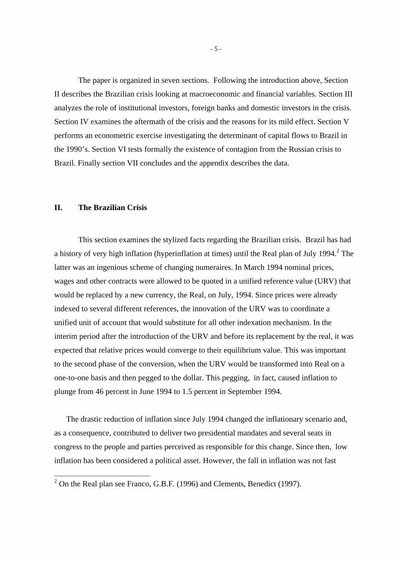
This section examines the stylized facts regarding the Brazilian crisis. Brazil has had
a history of very high inflation (hyperinflation at times) until the Real plan of July 1994.2 The
latter was an ingenious scheme of changing numeraires. In March 1994 nominal prices,
wages and other contracts were allowed to be quoted in a unified reference value (URV) that
would be replaced by a new currency, the Real, on July, 1994. Since prices were already
indexed to several different references, the innovation of the URV was to coordinate a
unified unit of account that would substitute for all other indexation mechanism. In the
interim period after the introduction of the URV and before its replacement by the real, it was
expected that relative prices would converge to their equilibrium value. This was important
to the second phase of the conversion, when the URV would be transformed into Real on a
one-to-one basis and then pegged to the dollar. This pegging, in fact, caused inflation to
plunge from 46 percent in June 1994 to 1.5 percent in September 1994.
The drastic reduction of inflation since July 1994 changed the inflationary scenario and,
as a consequence, contributed to deliver two presidential mandates and several seats in
congress to the people and parties perceived as responsible for this change. Since then, low
inflation has been considered a political asset. However, the fall in inflation was not fast
2 On the Real plan see Franco, G.B.F. (1996) and Clements, Benedict (1997).

- 6 -
enough to avoid a real appreciation of the exchange rate that prompted the central bank to set
an adjustable band for the dollar value of the real and maintain a continuing crawling peg
within it from 1995-1999 (see Figure 1). Notwithstanding the crawling peg that was set at
approximately 7 percent per year, the real exchange rate remained clearly overvalued as can
be seen from the increasing current account deficits (from around 2 percent in 1995 to 4.5
percent in 1998). The overvaluation contributed to the lack of GDP growth (see Table 1).
On top of the lack of competitiveness and poor GDP growth, fiscal performance
deteriorated in 1997 and 1998 which led the Brazilian economy to be vulnerable to external
shocks. There were three major external shocks after the Real plan, the Tequila effect in
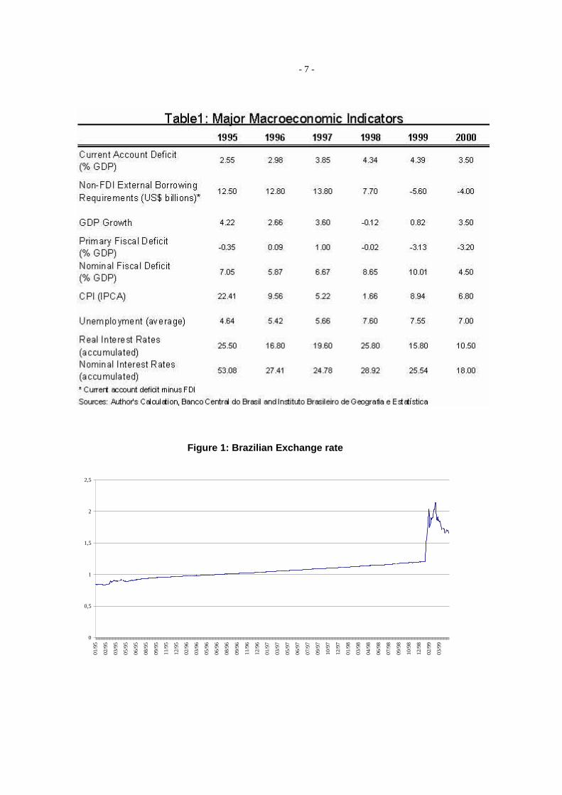
1995, the Asian crisis in 1997 and the Russian crisis in 1998. The reaction to the crisis was
similar in all cases. Nominal interest rates were doubled (see Figure 2) and a fiscal package
promised. This strategy was successful in averting a crisis after the Tequila and Asia shocks.
However, after the Russian crisis, this same strategy had a perverse effect. Instead of
attracting capital, the strategy this time induced capital outflows. The reason was that the
fiscal package was not credible and the higher interest rates increased nominal fiscal deficits
and raised fears of a sovereign default. As a consequence, large withdrawals followed and the
currency came under pressure.
- 7 -
Figure 1: Brazilian Exchange rate
0
0,5
1
1,5
2
2,5
01/9
5
02/9
5
03/9
5
05/9
5
06/9
5
08/9
5
09/9
5
11/9
5
12/9
5
02/9
6
03/9
6
05/9
6
06/9
6
08/9
6
09/9
6
11/9
6
12/9
6
01/9
7
03/9
7
05/9
7
06/9
7
07/9
7
09/9
7
10/9
7
12/9
7
01/9
8
03/9
8
04/9
8
06/9
8
07/9
8
09/9
8
10/9
8
12/9
8
02/9
9
03/9
9

- 8 -
Figure 2: Brazilian interest rates
0.00
10.00
20.00
30.00
40.00
50.00
01/9
7
01/9
7
02/9
7
03/9
7
04/9
7
04/9
7
05/9
7
06/9
7
07/9
7
07/9
7
08/9
7
09/9
7
09/9
7
10/9
7
11/9
7
12/9
7
12/9
7
01/9
8
02/9
8
03/9
8
03/9
8
04/9
8
05/9
8
06/9
8
06/9
8
07/9
8
08/9
8
08/9
8
09/9
8
10/9
8
11/9
8
11/9
8
12/9
8
01/9
9
02/9
9
02/9
9
03/9
9
04/9
9
AsianCrisis Russian
Crisis
BrasilianCrisis
The crisis was triggered by foreign investors that were exposed to Russian risk and
suffered major losses from both the restructuring of the Russian debt or/and the devaluation
of the Ruble. Others were surprised by the fact that it occurred within an IMF program and
panicked regarding other emerging markets. The effect on the exchange market in Brazil was
extreme. On August and September alone, the excess demand for dollars in the foreign
exchange market was 11,8 and 18,9 billion dollars, respectively. This obviously implied a
huge loss of reserves during these months and the following one (see Figure 3).
Analyzing the composition of flows at that time is interesting. Table 2 and Figure 4
show that the crisis hit very hard net portfolio flows and debt securities that deepened
immediately after the Russian crisis and only recovered in late 1999. In contrast, the share of
net direct investment increased steadily surpassing $20 billion in 1998 and $25 billion in
1999. This would suggest that the crisis is driven (or at least validated) by outflows of equity
and debt securities that are more volatile and react strongly during crisis, at least when

- 9 -
compared with direct investment flows. This gives support to the notion that policy makers
should use caution when the economy’s external accounts are financed by more volatile
flows (this call for caution often includes support for capital controls to put some “sands on
the wheels” on the swiftness of these flows).
Figure 3: Foreign Exchange Market and Reserve Movements
-25000
-20000
-15000
-10000
-5000
0
5000
10000
15000
07/9
5
09/9
5
11/9
5
01/9
6
03/9
6
05/9
6
07/9
6
09/9
6
11/9
6
01/9
7
03/9
7
05/9
7
07/9
7
09/9
7
11/9
7
01/9
8
03/9
8
05/9
8
07/9
8
09/9
8
11/9
8
01/9
9
03/9
9
05/9
9
07/9
9
09/9
9
11/9
9
US
$ M
illio
ns
Reserve Changes Foreign Exchange Market Balance
1991 1992 1993 1994 1995 1996 1997 1998 1999Net Direct Investement -408 1268 -481 852 2376 9519 15364 22988 25946 -FDI 505 1156 397 117 5475 10349 17086 26134 27109 -Reinvestment 365 175 100 83 384 531 151 124 NA -NBI -913 112 -878 -1065 -1560 77 -1569 -3212 -1163Net Portfolio Securities 578 1704 6651 7280 2294 6040 5300 -1861 1529Debt Securities 2368 5761 5866 3713 3113 12727 19771 28968 -7982Short term Capital and Others -7406 -2844 -4432 -3825 21523 4856 -15517 -30032 NATotal -4868 5889 7604 8020 29306 33142 24918 20063 NAReserve Changes -567 14348 8457 6595 13034 8270 -7937 -7616 -8214Current account deficit 1407 6144 592 1688 17972 23136 30916 33611 24378Source: Banco Central do Brasil
Note: FDI and NBI stand for Foreign and Brazilian direct investment, respectively. Portfolio investment,
comprise investment in equity securities (Annex I-VI) and funds. Debt securities include medium
and long term loans and financing. Short term capital and others equals the IFS “Financial Account”
minus the sum of direct investment, equity securities and debt securities.
Table 2 : Capital Flows

- 10 -
Figure 4. Composition of Capital Flows6 month moving average
-2500
-1500
-500
500
1500
2500
3500
4500
06/8
8
12/8
8
06/8
9
12/8
9
06/9
0
12/9
0
06/9
1
12/9
1
06/9
2
12/9
2
06/9
3
12/9
3
06/9
4
12/9
4
06/9
5
12/9
5
06/9
6
12/9
6
06/9
7
12/9
7
06/9
8
12/9
8
06/9
9
US
$ m
illio
ns
Net Direct Investment Net Portfolio Securities Debt Securities
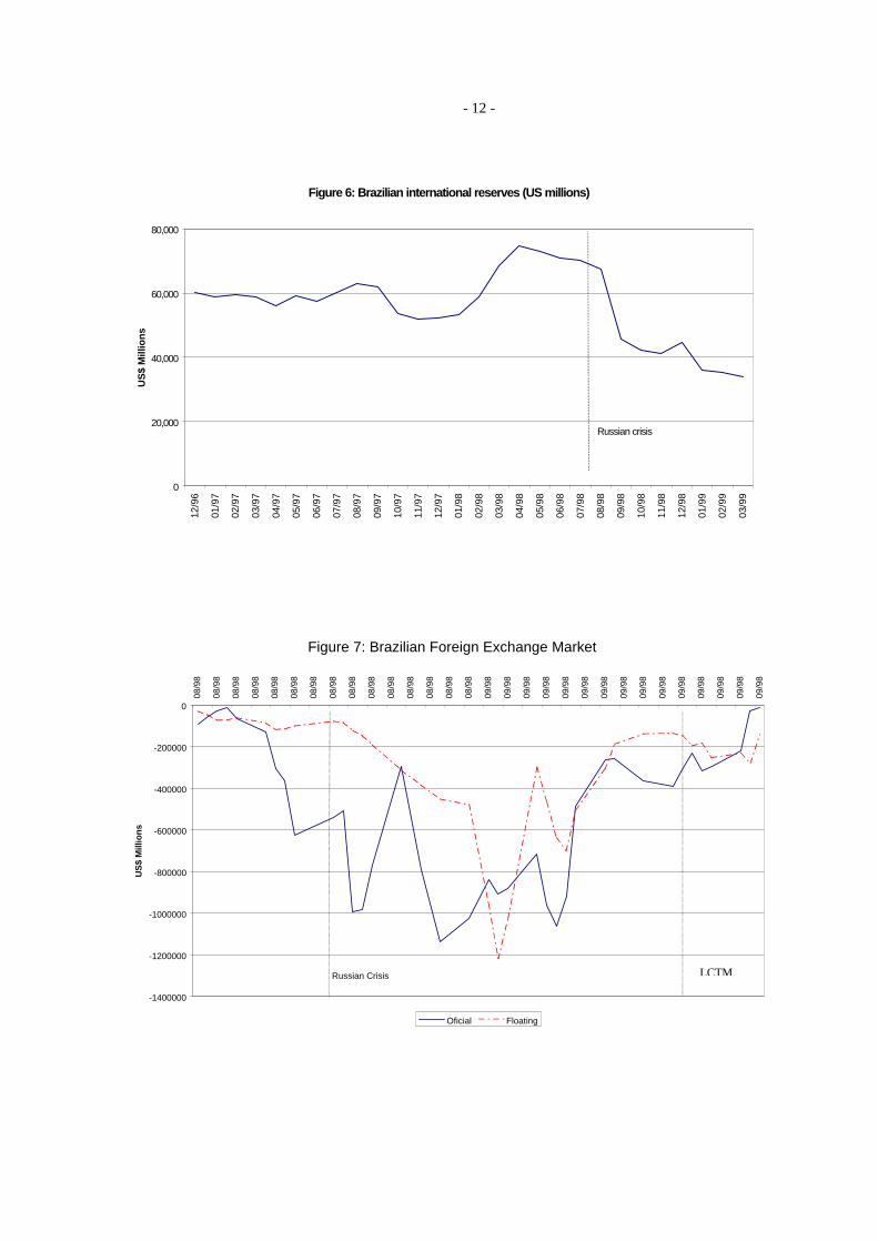
The effect of fast outflows can be observed on the movement of reserves and spreads
on Brady bonds in Figures 5-6. It is important to remember than in pegged regimes (or
crawling pegs), the appropriate variables to infer pressure are indeed either reserve
movements or interest rate levels. The latter are better used when looking at non-policy
interest rates, that are more market determined and less influenced by short term objectives of
policy makers.
With daily data, one can check the alternative hypothesis that it was the liquidity
crisis in mature markets that timed the crisis in Brazil and not the Russian crisis. The LTCM
crisis deepened along September 1998 (the rescue plan was announced the 23rd of the month)
while the Russian default happened a month earlier, on August 17. Figures 5 and 7 reveal
that most of the action happens immediately after the Russian crisis both in the foreign
exchange market and the brady bond one, although the spreads on the latter market suffer a
new blow during the LTCM crisis, specially the shorter maturity Brazilian IDU bond. Rather

- 11 -
than concluding in favor of LTCM effect on this market, the fact that the reaction occurs a
couple of weeks before the LTCM crisis is revealed and the behavior of withdrawals, leads
us to favor instead the argument that the Brazilian residents reinforced the speculation once
they realize that the speculation now included also foreign and institutional investors.
Other Brazilian financial variables reflect the Russian crisis with different lags. The
floating of the exchange rate occurred only in January, 1999, five months after the Russian
crisis. At the beginning, interest policy rate (overnight rate on federal funds - SELIC) was
raised to levels close to the ones reached during the Asian crisis, but this time speculation
forced the change in the exchange regime.
Russiancrisis
Spreads (C- Bonds)
0
200
400
600
800
1000
1200
1400
1600
01/0
1/97
01/0
2/97
01/0
3/97
01/0
4/97
01/0
5/97
01/0
6/97
01/0
7/97
01/0
8/97
01/0
9/97
01/1
0/97
01/1
1/97
01/1
2/97
01/0
1/98
01/0
2/98
01/0
3/98
01/0
4/98
01/0
5/98
01/0
6/98
01/0
7/98
01/0
8/98
01/0
9/98
01/1
0/98
01/1
1/98
01/1
2/98
01/0
1/99
01/0
2/99
01/0
3/99
01/0
4/99
01/0
5/99
01/0
6/99
Russian Crisis
Figure 5:
BrazilianCrisis
- 12 -
Figure 6: Brazilian international reserves (US millions)
0
20,000
40,000
60,000
80,000
12/9
6
01/9
7
02/9
7
03/9
7
04/9
7
05/9
7
06/9
7
07/9
7
08/9
7
09/9
7
10/9
7
11/9
7
12/9
7
01/9
8
02/9
8
03/9
8
04/9
8
05/9
8
06/9
8
07/9
8
08/9
8
09/9
8
10/9
8
11/9
8
12/9
8
01/9
9
02/9
9
03/9
9
US
$ M
illio
ns
Russian crisis
Figure 7: Brazilian Foreign Exchange Market
-1400000
-1200000
-1000000
-800000
-600000
-400000
-200000
0
08/9
8
08/9
8
08/9
8
08/9
8
08/9
8
08/9
8
08/9
8
08/9
8
08/9
8
08/9
8
08/9
8
08/9
8
08/9
8
08/9
8
08/9
8
09/9
8
09/9
8
09/9
8
09/9
8
09/9
8
09/9
8
09/9
8
09/9
8
09/9
8
09/9
8
09/9
8
09/9
8
09/9
8
09/9
8
09/9
8
US
$ M
illio
ns
Oficial Floating
Russian Crisis LCTM
- 13 -
In sum, in this section we argued that Brazil was vulnerable to a crisis given its fiscal
policy and overvalued exchange rate. The timing of the crisis was given by an external event,
the Russian crisis, and triggered by large withdrawals of portfolio and debt securities assets
by both domestic and foreign investors. In the next section the paper concentrates on the
players involved trying to disentangle the relative role of foreign, domestic and institutional
investors.
III. The Role of Domestic, Foreign and Institutional Investors in theBrazilian Crisis
Different agents have played different roles in other crises in the past. During the debt
crisis of the 80’s, it is well known that the crisis involved predominantly traditional bank
loans. Bank overborrowing (and overlending) was at the heart of the crisis. In contrast, in
more recent Mexico and Thailand crises, institutional investors had a predominant role. Here
we investigate the players involved in the withdrawals of funds from Brazil during the crisis.
Table 3 is an attempt to disentangle the role of domestic, foreign and institutional
investors in the various phases of the Brazilian crisis. One can observe large withdrawals out
of Brazil from all agents involved, in particular after the Russian crisis and up to the
Brazilian crisis, in the first quarter of 1999. The magnitudes are overwhelming. Institutional
investors withdrew U$ 13.1 billion, Banks withdrew U$ 10.9, Brazilian investors withdrew
7.0 billion. In addition, large withdrawals in the amount of $16 billion from the so-called
CC5 accounts were observed during the same period.3 Therefore, in the case of Brazil one
3 These CC5 deposit accounts were created in the past to allow nonresidents to invest inBrazil. Their regulations are very lax, but they are subject to high taxes. In practice they areowned predominantly by Brazilian residents disguised as residents of other countries.Foreign investment is mostly channeled through special fixed income and equity funds withlower tax incidence. Therefore, in the past few years there are only withdrawals from thestock of CC5 accounts.

- 14 -
cannot assert that a particular investor group had a predominant role in the crisis. If anything,
Brazilians were responsible for a large share of the withdrawals, if one includes the CC5
accounts.
In Table 3, one can observe the relative behavior of the players in the last few years.
It is clear that institutional investors (and also foreign banks) had a very atypical behavior
during the Russian crisis. It is interesting to compare with what occurred after the Asian
crisis. During that period the speculation against the currency was concentrated in the CC5
accounts. The withdrawals from both institutional investors and foreign banks were rather
modest, specially if compared with the effect of the Russian crisis. This raises the hypothesis
that while foreign investors (both banks and institutional investors) were long in Brazil, the
speculation against the currency was not overwhelming and Brazilian policy makers could
sustain withdrawals from Brazilians investors running from fear of devaluation. Once the
position of foreign investors changed, the balance of forces was altered and the currency peg
could no longer be sustained (although it took long 5 months from the Russian crisis to the
Brazilian devaluation).
Period Institutional Investors 1/
Brazilians 2/
Banks3/
Companies Other Foreign4/
CC5 Operations 5/
Annual Average 96-99
2,752 -2,598 -2,177 2,645 10,381 -17,356
Asian Crisis -1,725 -1,192 -271 1,616 -1,226 -12,445 Russian Crisis -10,601 -4,965 -6,889 815 5,502 -12,580
Brazilian Crisis -2,567 -2,025 -3,999 1,617 -6,398 -4,315Dec 98 -1,008 -175 -1,665 1,130 -629 -1,774Jan 99 -1,606 -1,367 -1,916 307 -706 -2,019Feb 99 47 77 -417 180 -5,062 -5221999 1,522 -1,951 -1,990 1,398 1,520 -10,373
1/ Portfolio Investment.2/ Portfolio investment plus medium and long term flows.3/: Net Medium and Long Term Loans to Banks and Credit Lines (Short Term)4/: Includes Medium and Long Term Bonds, Commercial Papers, Notes, Securitization and Others5/: Operations with non-resident accounts.Note: Asian Crisis from August/1997 to December/1997; Russian Crisis from August/1998 to October/1998. Brazilian Crisis from December/1998 to February/1999Source: Banco Central do Brasil
Table 3: Net Inflows to Brazil by Type of Investor (in U$ Millions)

- 15 -
Further information may be obtained from movements in the dual foreign exchange
market. At the time of the crisis, the central bank was setting an adjustable band for the dollar
value of the real and maintained a continuing crawling peg within it. There were two foreign
exchange markets, the “official” and the floating market. Their difference was given by the
type of transaction allowed. In the official market mostly proceeds of exports and imports of
goods and services were allowed but also a few capital account transactions. One important
example is most of the portfolio investment by foreign investors which was channeled either
through two classes of fixed-income funds or through one of the five alternatives established
under National Monetary Council Resolution 1289. In the floating market most of the rest
of the capital account transactions was transacted, in particular, those made by Brazilian
residents. The Brazilian government would keep the exchange rates on both markets aligned
and would not allow big differences between them.
It is clear from Table 4 that the extent of withdrawals in the in the official market
during the Russian crisis was severe, reflecting withdrawals from foreign investors. This is in
contrast to their behavior through the Asian crisis, where the withdrawals were about the
average for this market. On the other hand, the floating markets had already showed large
withdrawals during the Asian crisis but were reversed a few months later. During the Russian
crisis the large withdrawals did not reversed and were fueled by fears from parallel
withdrawals in the official markets. Therefore from the dimension of the players involved,
the information obtained from the two separate exchange markets would suggest that, in fact,
the withdrawals from foreign investors made the difference in terms of the effect of the
Russian crisis relative to the Asian crisis. This contributes to the hypothesis that the
contagion from Russia was triggered by foreign investors panicking from the Russian crisis.
The floating market investors, that include Brazilian residents, had already jump chip during
the Asian crisis and repeated the pattern during the Russian crisis, which, of course,
contributed to the pressure in the exchange markets

- 16 -
Floating Market rate Official Rate Exchange Rate Foreign Res.ChangesAverage Jul/95 - Jul/98 -1,322 2,670 1,348 992Average Aug/98 - Dez/98 -3,601 -4,327 -7,928 -6,996Average Jul/95 - Nov/99 -1,593 1,324 48 -198
Set/97 -1,651 613 -1,038 -1,125Out/97 -4,912 -1,039 -5,951 -8,241Nov/97 -3,700 -292 -3,992 -1,655
Jul/98 -1,839 6,693 4,855 -688Ago/98 -2,821 -8,989 -11,810 -2,877Set/98 -8,578 -10,348 -18,926 -21,522Out/98 -2,867 971 -1,896 -3,426
Source: Banco Central do Brasil
In Millions of US Dollars
Asia Crisis
Russia Crisis
Table 4: Brazilian Foreign Exchange Market
Therefore, we are confirming in this section that although the Brazilian economy was
vulnerable to shocks and Brazilian investors were always prone to withdraw their funds
from their country, the timing of the crisis was given by the Russian crisis and from the
withdrawals of foreign investors, in particular, institutional investors.
The Role of International Banks in the Crisis
Throughout the crisis, foreign investors reduced their exposure to Brazil, as
maturing obligations came due. Tracking this process may give us information regarding
the players involved in the crisis. The Central Bank of Brazil follows the maturing short
term external liabilities of its banking system in a weekly basis. The short term
obligations include interbank and credit lines. This survey based monitoring system was
introduced on October 1998, after the Russian crisis and during the negotiations with the
IMF.
Table 5 shows the cumulative reduction in short term exposure to Brazilian banks by
nationality. Over the sample period the rolled over portion was $4 out of the total $6,6
billion that was maturing, amounting to a rollover rate of around 62%. U.S. banks reduced
their exposure by US$931 million, with a rollover rate of 60%. Within the US, the reduction
in exposure was concentrated, but nonetheless widespread. Almost one-half of the reduction
came from two banks and ten banks accounted for 84 percent of the total decline. As
expected, many regional banks reduced their exposure.

- 17 -
The rollover rate for US banks was well below the rollover rates of Germany (79
percent) and the UK (77 percent), although it was roughly in line with Japan (58 percent),
France (54 percent) and Italy (60 percent). This is interesting because it bears on our
fundamental question regarding the contagion from Russia to Brazil and the hypothesis that
liquidity needs and withdrawals were one of channels of contagion. German banks had a
larger exposure to Russia, were badly affected by the Russian crisis, and had the largest
maturing amount of debt after the US. Their rollover rate, however, does not reflect a
compensatory liquidation of assets since it is far above average.
The fact that the data does not support a common lender channel through Germany
does not contradict our previous finding that foreign investors triggered the Brazilian crisis.
The common lender is just one of possible channels of contagion. It could well be the case
that foreign investors adjusted their probability of Brazilian default once they observed the
Russian crisis (for example, because of a default under an IMF program) or the Russian
crisis could have triggered a pure herding behavior by foreign investors.
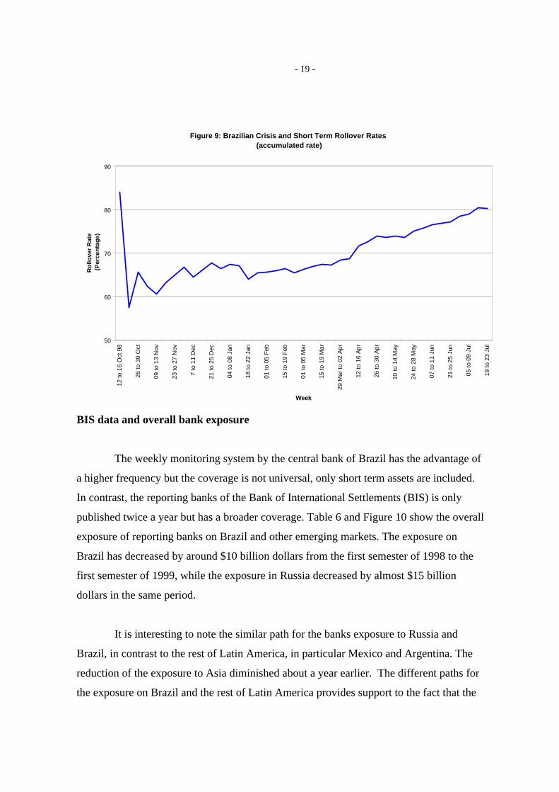
The frequency of the data also allows us to follow the timing of the reduction of
exposure, although with a lag given that the first data is from the third week of October.
Figures 8-9 show the net outflows per week and the rollover rate over time. The weekly
changes in exposure have been volatile, with a particularly sharp deterioration in October
and over the final two weeks of the year, which was a end-year window dressing. The high
rollover weeks happen in April after the Brazilian agreement with international banks to
maintain short term lines. For the 11-week monitoring period ending January 1, 1999, the
aggregate rollover rate was 72 percent. The weekly observations, however, have been
volatile, ranging from 50 percent to 90 percent. It is interesting also to note that the
international banks has not increased the exposure to their previous level before the Russian
crisis. This is in part due to lack of demand for short term borrowing by Brazilian banks
after the floating of the exchange rate and the associated higher exchange rate risk.

- 18 -
Maturing $ Rolled Over Rollover RateUSA 2352 1421 0.60Canada 168 74 0.44France 947 516 0.54Germany 1060 835 0.79Italy 215 129 0.60Japan 715 416 0.58Netherlands 222 69 0.31Portugal 97 90 0.93Spain 350 145 0.41UK 505 389 0.77Total 6630 4082 0.62
* From October to December 1998
Source: BIS
In Millions of Dollars
Table 5: Changes in Exposure of Short Term Loans (Interbank + Trade) to Brazil*
Figure 8: Brazilian Weekly Short Term Bank Loans
-1000
-800
-600
-400
-200
0
200
400
600
12 to
16
Oct
98
26 to
30
Oct
09 to
13
Nov
23 to
27
Nov
7 to
11
Dec
21 to
25
Dec
04 to
08
Jan
18 to
22
Jan
01 to
05
Feb
15 to
19
Feb
01 to
05
Mar
15 to
19
Mar
29 M
ar to
02
Apr
12 to
16
Apr
26 to
30
Apr
10 to
14
May
24 to
28
May
07 to
11
Jun
21 to
25
Jun
05 to
09
Jul
19 to
23
Jul
Week
Mill
ion
s o
f U
$
* Short term interbank and trade credit lines
- 19 -
Figure 9: Brazilian Crisis and Short Term Rollover Rates (accumulated rate)
50
60
70
80
90
12 to
16
Oct
98
26 to
30
Oct
09 to
13
Nov
23 to
27
Nov
7 to
11
Dec
21 to
25
Dec
04 to
08
Jan
18 to
22
Jan
01 to
05
Feb
15 to
19
Feb
01 to
05
Mar
15 to
19
Mar
29 M
ar to
02
Apr
12 to
16
Apr
26 to
30
Apr
10 to
14
May
24 to
28
May
07 to
11
Jun
21 to
25
Jun
05 to
09
Jul
19 to
23
Jul
Week
Ro
llove
r R
ate
(P
erce
nta
ge)
BIS data and overall bank exposure
The weekly monitoring system by the central bank of Brazil has the advantage of
a higher frequency but the coverage is not universal, only short term assets are included.
In contrast, the reporting banks of the Bank of International Settlements (BIS) is only
published twice a year but has a broader coverage. Table 6 and Figure 10 show the overall
exposure of reporting banks on Brazil and other emerging markets. The exposure on
Brazil has decreased by around $10 billion dollars from the first semester of 1998 to the
first semester of 1999, while the exposure in Russia decreased by almost $15 billion
dollars in the same period.
It is interesting to note the similar path for the banks exposure to Russia and
Brazil, in contrast to the rest of Latin America, in particular Mexico and Argentina. The
reduction of the exposure to Asia diminished about a year earlier. The different paths for
the exposure on Brazil and the rest of Latin America provides support to the fact that the

- 20 -
contagion from the Russian crisis was not generalized, as it would be if driven only by
liquidity needs.
Brazil Mexico Russia Argentina97.1 71862 62161 69081 4484497.2 76292 61794 72173 6041398.1 84585 62892 75853 6022298.2 73313 64962 58594 6151799.1 62310 63776 55424 66683
in billions of dollars
Table 6: BIS Banks Holding (US$) in Emerging Markets Data
Figure 10: BIS Banks Holdings in Emerging Markets
80
120
160
95.1 95.2 96.1 96.2 97.1 97.2 98.1 98.2 99.1
ind
ex 9
4.2=
100
Mexico
Asia Brazil
Russia Latin America
j
- 21 -
In this section, we analyzed in more detail the behavior of foreign investors. All the
players reduced their exposure to Brazil after the Russian crisis. We concluded that although
there was a contagion from Russia (more formal tests in section VI), the channel was
probably not through a common lender. In the next section, we continue our analysis of the
Brazilian crisis focusing on the aftermath of the crisis.
IV. The Aftermath of the Crisis – 1999
Brazil’s macroeconomic performance during the crisis year was better than expected.
Inflation did not explode, GDP did not collapsed, the government was not forced to
restructure its public debt and, slowly, both nominal and real interest rates have been going
down (see Table 1). This performance is partly due to the fact that the private sector was
largely hedged at the moment of the crisis and was insulated from the immediate effects of
the devaluation. In fact, the government born most of the costs of the devaluation by having
its public debt increase by around 10 percent of GDP. Since debts have eventually to be paid,
or at least not allowed to explode, the better than expected performance have to be judged
against the feasibility of generating current and future fiscal surpluses in a country where
sustained growth is long overdue and fiscal consolidation a novelty.
Brazil’s better than expected macroeconomic performance has been achieved partly
due to a more responsible fiscal policy. In the past Brazil has inflated its way out of past
fiscal inconsistencies, using inflation as the means to finance deficits that otherwise could not
be financed. The consequences were dear, inflation reached more than 1000 percent per cent,
growth stalled and income distribution deteriorated substantially. This time Brazil has
fulfilled the IMF-agreed target as shown in Table 7. Figure 11 shows that this effort could be
successful in stabilizing the debt to GDP ratio, if sustained.
In contrast to the generalized expectation, inflation was extremely moderate in 1999,
notwithstanding the large nominal depreciation that followed the floating of the exchange
rate. Consumer price index (IPCA) increased only 9 percent this year and the expectations
are of a 7 percent inflation next year. Of course, the exchange rate depreciation has a larger
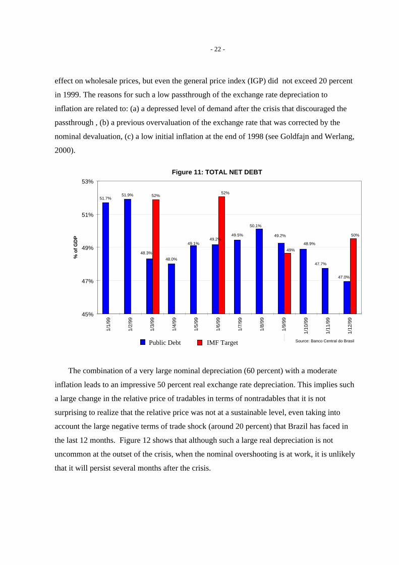
- 22 -
effect on wholesale prices, but even the general price index (IGP) did not exceed 20 percent
in 1999. The reasons for such a low passthrough of the exchange rate depreciation to
inflation are related to: (a) a depressed level of demand after the crisis that discouraged the
passthrough , (b) a previous overvaluation of the exchange rate that was corrected by the
nominal devaluation, (c) a low initial inflation at the end of 1998 (see Goldfajn and Werlang,
2000).
Figure 11: TOTAL NET DEBT
51.7%51.9% 52%
47.0%
48.9%
49.2%
47.7%
49.1%
48.3%
48.0%
49.2%49.5%
50.1%
50%
49%
52%
45%
47%
49%
51%
53%
1/1/
99
1/2/
99
1/3/
99
1/4/
99
1/5/
99
1/6/
99
1/7/
99
1/8/
99
1/9/
99
1/10
/99
1/11
/99
1/12
/99
% o
f G
DP
Dívida Pública Meta FMI Source: Banco Central do Brasil
The combination of a very large nominal depreciation (60 percent) with a moderate
inflation leads to an impressive 50 percent real exchange rate depreciation. This implies such
a large change in the relative price of tradables in terms of nontradables that it is not
surprising to realize that the relative price was not at a sustainable level, even taking into
account the large negative terms of trade shock (around 20 percent) that Brazil has faced in
the last 12 months. Figure 12 shows that although such a large real depreciation is not
uncommon at the outset of the crisis, when the nominal overshooting is at work, it is unlikely
that it will persist several months after the crisis.
Public Debt IMF Target

- 23 -
IMF-Targets
1998 4,845 (1,562) (3,170) 113 Jan/99 2,155 304 78 2,537 Fev/99 3,931 454 709 5,094 Mar/99 7,315 902 1,478 9,694 Abr/99 8,564 1,484 743 10,791 Mai/99 8,622 1,839 1,266 11,726 Jun/99 12,536 1,978 961 15,475 12,883 Jul/99 16,267 2,050 2,107 20,424 15,626
Ago/99 19,264 1,798 4,110 25,172 20,590 Set/99 22,868 2,652 5,054 30,574 23,788 Out/99 23,643 3,064 5,335 32,042 26,078 Nov/99 24,018 3,721 5,159 32,899 27,763 Dez/99 22,676 2,118 6,317 31,112 30,185
Source: Banco Central do Brasil
Table 7: Primary Accumulated Deficit
Observed
TOTALTOTALPublic
enterprisesMunicipal & State Gov.
FEDERAL GOV. & BACEN
Figure 12: Real Exchange Rate - Selected Crises Casesday before crises=100
90
100
110
120
130
140
150
160
170
180
190
200
210
220
0 10 20 30 40 50 60 70 80 90 100
110
120
130
140
150
160
170
180
190
200
210
220
230
240
250
260
270
280
290
300
310
320
330
340
350
360
370
380
390
400
410
420
430
440
450
460
470
480
490
500
working days
Brazil
South Korea
Mexico
Source: Bloomberg

- 24 -
There are two ways to correct an undervalued exchange rate: with a nominal appreciation,
through higher inflation or a combination of the two. Figure 13 illustrates the two
possibilities that were available to Brazil, a Korea-style nominal appreciation or a Mexican-
style depreciation-inflation spiral. Initially it seems that Brazil would follow the path with
low inflation and a bit of appreciation but the Mexican path is always possible.
In fact, the observed reversal of the real exchange rate through either inflation (Mexico)
or appreciation (Korea) is a more general phenomena. In several crisis cases, the degree of
passthrough, the ratio of inflation to nominal depreciation, has increased systematically
throughout the crisis . Figure 14 reveals that for 9 crisis cases in the recent past, either
depreciation increased or inflation picked up, leading to a higher passthrough starting 6
months after the crisis. It seems that Brazil is following this trend.
In the next two sections, we perform our econometric exercises, first on capital flows and
then testing contagion from Russia.
Figure 13: Nominal Exchange Rate - Selected Crises Casesday before crises=100
90
100
110
120
130
140
150
160
170
180
190
200
210
220
230
240
0 10 20 30 40 50 60 70 80 90 100
110
120
130
140
150
160
170
180
190
200
210
220
230
240
250
260
270
280
290
300
310
320
330
340
350
360
370
380
390
400
410
420
430
440
450
460
470
480
490
500
working days
Brazil
South Korea
Mexico
Source: Bloomberg

- 25 -
V. Capital Flows to Brazil in the 1990’s: Econometric Analysis
We now investigate the determinants of capital flows to Brazil. The ordinary least
squares (OLS) regression controlling for heteroscedasticity and serial correlation is:
where nf, i, i*, Ee are the net capital flows as a percentage of GDP, the domestic interest rate,
the foreign interest rate, and expected devaluation, respectively, and X is a group of variables
including domestic variables such as inflation, government spending, the real exchange rate,
and a series of dummies for the Real Plan, the Tequila effect, the Asian crisis, the Brazilian
crisis, and the Russian crisis . The data is in monthly frequency (see the appendix for formal
definitions of the variables). The results are summarized in Table 8 - 9 below.
As predicted by theory, the coefficient of the international interest rate is negative and
significant. This result is consistent with evidence for Latin America in Calvo and others
Figure 14: Pass-through, Effect of devaluation on inflation (%)
0%
10%
20%
30%
40%
50%
60%
70%
80%
Italy Sweeden UnitedKingdom
Mexico SouthKorea
Malaysia Indonesia Thailand Brazil
Currency Crises Cases
Infla
tion
over
Dev
alua
tion
%
12 months24 months
Korea with only 22 months

- 26 -
(1993), and with evidence f or developing countries in Fernández-Arias and Montiel (1995).
The result is robust across specifications and to using either returns on U.S. Treasury bills or
yields on 10-year Treasury bonds. The coefficient of the domestic interest rate adjusted for
expected depreciation and the coefficients of other domestic factors do not help in explaining
capital flows to Brazil. We interpret the results as evidence in favor of push effects as
opposed to pull effects in explaining the surge in capital flows in the 1990’s.
This result does not contradict our previous assertion that Brazil was vulnerable to a
crisis and that the timing of the crisis was given by sudden large withdrawals of capital. The
determinants of capital flows to Brazil in the long run are dominated by pull effects (foreign
interest rates) but the composition of flows were determined by weak Brazilian fundamentals.
In fact, the composition of capital flows was concentrated on short term portfolio flows that
are prone to sudden spikes in capital flows. A better macroeconomic environment would
imply a larger proportion of FDI in the overall capital flows (Figure 3 confirms that this is the
case since 1999).
The dummies for the Tequila and Real plan are strong and significant. The Russian
crisis has a strong negative coefficient but it is not statistically significant. This lack of
significance is a bit surprising, since in sections II and III, in the higher frequency data, we
observed a large withdrawal of capital during the Russian crisis. However, from a longer
term perspective the Russian crisis did not in fact change the flows to the Brazilian economy.
Capital inflows recovered and there was an important change in the composition of capital
flows to Brazil with net foreign investment replacing other component of flows and partially
dampening the effect of the Russian crisis.4
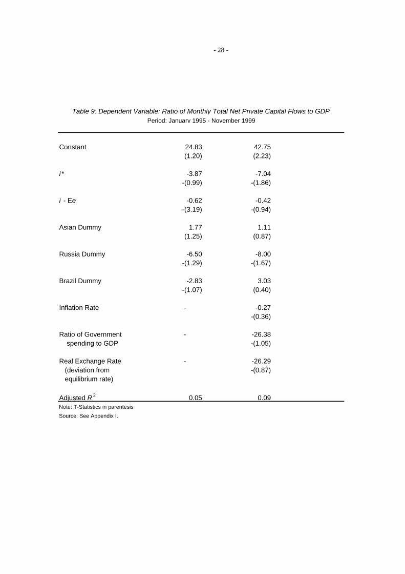
It is interesting to observe that in the period 1995-1999, in Table 9, the coefficient on
international interest rate loses its significance. This suggests that the push effects have a
4 The analysis and econometric regressions of the components of capital flows may be
obtained directly from the author.

- 27 -
more long run effect, affecting capital flows only once large changes in international interest
rates are factored in.
Constant 4.78 4.95 5.28(5.05) (5.14) (2.69)
i * -0.64 -0.68 -0.79-(4.60) -(4.68) -(3.13)
i - Ee -0.01 -0.13 0.02-(0.62) -(0.64) (0.50)
Tequila Dummy -5.65 -5.96 -6.07-(5.60) -(5.43) -(5.33)
Real Plan Dummy 2.47 2.78 2.49(2.98) (2.99) (2.46)
Asian Dummy 2.73 2.41 2.42(2.99) (2.42) (2.42)
Russia Dummy - -4.60 -4.86-(1.63) -(1.54)
Brazil Dummy - -0.56 -0.09-(0.47) -(0.06)
Inflation Rate - - 0.01(0.28)
Ratio of Government - - 2.38 spending to GDP (0.24)
Real Exchange Rate - - -2.48(deviation from -(0.55)equilibrium rate)
Adjusted R 2 0.24 0.26 0.25Note: T-Statistics in parentesis
Source: See Appendix I.
Table 8: Dependent Variable: Ratio of Monthly Total Net Private Capital Flows to GDPPeriod: January 1988 - November 1999
- 28 -
Constant 24.83 42.75(1.20) (2.23)
i * -3.87 -7.04-(0.99) -(1.86)
i - Ee -0.62 -0.42-(3.19) -(0.94)
Asian Dummy 1.77 1.11(1.25) (0.87)
Russia Dummy -6.50 -8.00-(1.29) -(1.67)
Brazil Dummy -2.83 3.03-(1.07) (0.40)
Inflation Rate - -0.27-(0.36)
Ratio of Government - -26.38 spending to GDP -(1.05)
Real Exchange Rate - -26.29(deviation from -(0.87)equilibrium rate)
Adjusted R 2 0.05 0.09Note: T-Statistics in parentesis
Source: See Appendix I.
Table 9: Dependent Variable: Ratio of Monthly Total Net Private Capital Flows to GDPPeriod: January 1995 - November 1999

- 29 -
VI. Testing Contagion
In the previous sections, we argued that the timing of the Brazilian crisis was a
consequence of the contagion from Russia but we had not offered a formal tests of this
proposition. This section fills this gap using primarily the sovereign spreads. Analyzing the
currency market is not very useful as for most of the sample period, both the Brazilian Real
and the Russian Ruble were fixed to the dollar. The currencies move about relatively freely
only after January 1999 (when the Real peg unraveled), but that period leaves out many
important phases of the crisis.
In order to understand the transmission of shocks from Russia to Brazil, we carry out
a series of tests. We begin by looking at rolling correlations (at three month interval) between
the relevant variables. We use granger causality tests and reduced form VARs to examine the
direction of shocks between Russia and Brazil.
We then define crisis and tranquil periods, and test for significant changes in
correlations between the two periods. We apply the Forbes and Rigobon (1999) methodology
to adjust the crisis period correlations for sudden increase in variance (see Appendix). The
motivation for this approach is to control for the correlation bias associated with higher
variances, i.e. in the standard correlation formula, higher variances lead to higher
correlations. Once the adjustment is performed, crisis period correlations can be tested for
significant increases without the potential of this bias. We use the Forbes and Rigobon test
with caution, as we are not sure a study of contagion ought to control for the increased
variances that are an integral part of any crisis scenario. It could very well be that the factors
behind the increased variances (thin markets, panic, institutional failure, etc.) are precisely
what make up contagion, and controlling for these factors make test for contagion moot.
The tranquil period sovereign spreads correlations are substantially larger than what
we saw in the stock market case. Using 106 observations from January – May, 1997, we find

- 30 -
the correlation to be 0.35. The spreads of both the bonds in discussion shot up even further
in the crisis period (see Figure 15). The correlation of the spreads also jumped (see Table 10),
and remained at very high levels till late 1998. The direction of the shock goes both ways, as
at various periods the two markets appear to be Granger Causing each-other (see Table 11).
Table 10: Brazil-Russia Correlations(Sovereign Spreads)
DateNo. of Obs.
Unadjusted Correlation
Adjusted Correlation
t-stat
Tranquil Period
1/1997 5/1997 106 0.35
Crisis Period
Full Sample 09/1997 12/1998 335 0.94 0.32 -1.31
Three month windows 09/1997 11/1997 65 0.87 0.97 39.5510/1997 12/1997 66 0.82 0.94 33.0010/1997 01/1998 58 0.41 0.85 19.1112/1997 02/1998 57 0.51 0.93 27.2101/1998 03/1998 55 0.87 0.99 46.3401/1998 04/1998 62 0.86 0.99 54.6302/1998 05/1998 62 0.89 0.99 63.4204/1998 06/1998 62 0.91 0.97 40.6705/1998 07/1998 65 0.79 0.86 21.8006/1998 08/1998 66 0.98 0.67 10.7307/1998 09/1998 65 0.97 0.46 2.9807/1998 10/1998 64 0.85 0.27 -2.1709/1998 11/1998 63 0.29 0.50 4.2310/1998 12/1998 65 -0.03 -0.02 -9.04
Source: Bloomberg
bold denotes significance at 10% or lower
Impulse response function from the VARs show large and persistent shocks
transmitting from both countries during the crisis period. The adjusted correlations for the
spreads show significantly higher correlation during the crisis period sub-samples when
compared to the tranquil period (see Table 10). All but two sub-samples in the crisis period

- 31 -
had significantly higher adjusted correlations. This confirms our findings from previous work
(Baig and Goldfajn, 1998) that the correlations in the Brady markets are very high and
increases significantly (even after the adjustment) during the crisis. This gives support to the
fact that if there was a contagion from Russia to Brazil, the most likely place of the
transmission was the off-shore Brady markets.
Table 11: Granger Causality Tests (Financial Flows)
Sample 1/1/97-5/30/97 9/1/97-11/28/97 10/01/1997-12/31/1997 10/31/1997-1/30/1998
Null Hypothesis: Obs F-Stat Prob. Obs F-Stat Prob. Obs F-Stat Prob. Obs F-Stat Prob.
FLF1 does not Granger Cause OFF1 89 1.33 0.27 65 1.39 0.26 63 0.62 0.54 60 0.18 0.84OFF1 does not Granger Cause FLF1 0.01 0.99 0.06 0.94 0.21 0.81 4.40 0.02
Sample 12/01/1997-2/27/1998 1/01/1998-3/31/1998 1/30/1998-4/30/1998 2/27/1998-5/29/1998
Null Hypothesis: Obs F-Stat Prob. Obs F-Stat Prob. Obs F-Stat Prob. Obs F-Stat Prob.
FLF1 does not Granger Cause OFF1 55 0.38 0.69 57 1.94 0.15 54 0.20 0.82 56 1.89 0.16OFF1 does not Granger Cause FLF1 0.06 0.94 1.66 0.20 1.34 0.27 1.36 0.27
Sample 4/01/1998-6/30/1998 5/01/1998-7/31/1998 6/01/1998-8/31/1998 7/01/1998-9/30/1998
Null Hypothesis: Obs F-Stat Prob. Obs F-Stat Prob. Obs F-Stat Prob. Obs F-Stat Prob.
FLF1 does not Granger Cause OFF1 52 1.96 0.15 60 1.45 0.24 63 2.88 0.06 63 2.62 0.08OFF1 does not Granger Cause FLF1 0.82 0.45 0.91 0.41 0.64 0.53 0.46 0.63
Sample 7/31/1998-10/30/1998 9/01/1998-11/30/1998 10/01/1998-12/31/1998 10/01/1998-12/31/1998
Null Hypothesis: Obs F-Stat Prob. Obs F-Stat Prob. Obs F-Stat Prob. Obs F-Stat Prob.
FLF1 does not Granger Cause OFF1 60 5.72 0.01 56 4.99 0.01 57 7.02 0.00 56 0.08 0.92OFF1 does not Granger Cause FLF1 0.45 0.64 0.88 0.42 1.52 0.23 0.99 0.38
OFF1: Official market financial net flows ( see section III)FLF1: Floating market net flows ( see section III)
Note: Significant (within 10 %) values are in bold)

- 32 -
Figure 15
Impulse Response Functions (from reduced-form VARs)Sovereign Spreads Response (to one S.D. Innovation)
Tranquil Period (01/01/1997 05/30/1997)
Response of Brazil to Russia Response of Russia to Brazil
Crisis Period (01/01/1998 12/31/1998)
Response of Brazil to Russia Response of Russia to Brazil
-2
0
2
4
6
10 20 30 40 50 60 70 80 90 100
-6
-4
-2
0
2
4
10 20 30 40 50 60 70 80 90 100
-10
0
10
20
30
40
10 20 30 40 50 60 70 80 90 100-100
0
100
200
300
400
500
10 20 30 40 50 60 70 80 90 100

- 33 -
IV. Conclusions
The paper has reached a few conclusions that are worth summarizing below. First,
we argued that Brazil was vulnerable to a crisis given its fiscal policy and overvalued
exchange rate. The timing of the crisis was given by an external event, the Russian crisis, and
triggered by large withdrawals of portfolio flows. In the case of Brazil one cannot assert that
a particular investor group had a predominant role in the crisis. If anything, the data suggest
that while foreign investors (both banks and institutional investors) were long in Brazil, the
speculation against the currency was not overwhelming and Brazilian policy makers could
sustain withdrawals from Brazilians investors running from fear of devaluation. Once the
position of foreign investors changed, the balance of forces was altered and the currency peg
could no longer be sustained.
Second, using weekly data on foreign banks exposure to Brazil from the central bank
of Brazil , we checked the hypothesis that liquidity needs and withdrawals were one of the
reasons that determined the timing of the Brazilian crisis. We observed that German banks
(known to have had a large exposure to Russia and were badly affected by the Russian
crisis) had one of the highest rollover rates within the G7 and, therefore, the data does not
seem to reflect a common lender channel through Germany. This does not contradict our
previous finding that foreign investors triggered the Brazilian crisis. The common lender is
just one of possible channels of contagion. It could well be the case that foreign investors
adjusted their probability of Brazilian default once they observed the Russian crisis (for
example, because of a default under an IMF program) or the Russian crisis could have
triggered a pure herding behavior by foreign investors.
Third, using daily data on several financial data from Bloomberg, one can check the
alternative hypothesis that it was the liquidity crisis in mature markets that timed the crisis in
Brazil and not the Russian crisis. However, most of the action happens immediately after the
Russian crisis both in the foreign exchange and the Brady bond markets, although the spreads
on the latter market suffer a new blow during the LTCM crisis. Therefore, rather than

- 34 -
concluding in favor of LTCM effect on this market, this leads us to favor instead the
argument that the Brazilian residents reinforced the speculation once they realize that the
speculation now included also the foreign investors.
Fourth, Brazil’s macroeconomic performance during the crisis year was better than
expected. Inflation did not explode, GDP did not collapsed, the government was not forced to
restructure its public debt and, slowly, both nominal and real interest rates have been going
down. This performance is partly due to the fact that the private sector was largely hedged at
the moment of the crisis and was insulated from the immediate effects of the devaluation. In
addition, the reasons for such a low passthrough of the exchange rate depreciation to inflation
are related to: (a) a depressed level of demand after the crisis that discouraged the
passthrough , (b) a previous overvaluation of the exchange rate that was corrected by the
nominal devaluation, (c) a low initial inflation at the end of 1998.
Fifth, the econometric exercise on capital flows suggests that there is evidence in
favor of push effects as opposed to pull effects in explaining the surge capital flows.
However, the push effects have a more long run effect, affecting capital flows only once
large changes in international interest rates are factored in. This result does not contradict our
assertion that Brazil was vulnerable to a crisis and that the timing of the crisis was given by
sudden large withdrawals of capital. The determinants of capital flows to Brazil in the long
run are dominated by pull effects (foreign interest rates) and the composition of flows were
determined by weak Brazilian fundamentals.
Finally, the econometric test of contagion from Russia shows that the comovement
between the variables is remarkable, specially with regards to the spreads on Brady bonds.
This confirms our findings from previous work (Baig and Goldfajn, 1998) that the
correlations in the Brady markets are very high and increase significantly (even after
adjusting for the bias) during the crisis. This gives support to the fact that if there was a
contagion from Russia to Brazil, the most likely place of the transmission was the off-shore
Brady markets.
- 35 -
Bibliography
Baig, T. and Goldfajn, I. “Financial Markets Contagion in the Asian Crisis,” IMF StaffPapers, 46, 167-195.
Baig, T. and Goldfajn, I. “The contagion from Russia to Brazil,” Working Paper No 420,Department of Economics at PUC, Rio de Janeiro.
Calvo, Guillermo, Leonardo Leiderman, and Carmen Reinhart, 1996, “Inflows of Capital toDeveloping Countries in the 1990s,” Journal of Economic Perspectives, Vol. 10,No. 2, pp. 123-39.
_____, 1993, “Capital Inflows to Latin America: The Role of External Factors,” Staff Papers,International Monetary Fund, Vol. 40 (March), pp. 108-51.
Cárdenas, Maurício, and Felipe Barrera, 1997, “On the Effectiveness of Capital Controls:The Experience of Colombia During the 1990s,” Journal of Development Economics,54(1) oct 97, pg 27-57, Fedesarrollo, Bogotá, Colombia).
Cardoso, Eliana, 1997, “Brazil’s Macroeconomic Policies and Capital Flows in the 1990s,”WIDER Project on capital flows in the 1990s (unpublished, January).
_____, and Goldfajn, I. “Capital Flows to Brazil: The Endogeneity of Capital Controls, ”IMF Staff Papers, 46, 167-195.
_____, and Rudiger Dornbusch, 1989, “Foreign Private Capital Flows,” in H.Chenery andT.N. Srinivasan, eds., Handbook of Development Economics (Amsterdam: North-Holland).
Claessens, Stijn, Michael Dooley, and Andrew Warner, 1995, “Portfolio Capital Flows: Hotor Cold?,” Harvard Institute for International Development: Development DiscussionPaper No. 501 (Cambridge, Massachusetts).
Clements, Benedict, 1997, ”The Real Plan, poverty and income distribution in Brazil”,Finance and Development, 34(3), sep 97, pg 44-46.
Dooley, Michael, 1995, “A Survey of Academic Literature on Controls over InternationalCapital Transactions,” Working Paper 95/127 (Washington: Internacional MonetaryFund).
_____, 1996, “Capital Controls and Emerging Markets,” International Journal of Financeand Economics, Vol. 1, No. 3 (July), pp. 197-206.

- 36 -
Fernández-Arias, Eduardo, and Peter Montiel, 1995, “The Surge in Capital Inflows toDeveloping Countries,” Policy Research Working Paper 1473 (Washington: WorldBank).
Folkerts-Landau, David, and Takatoshi Ito, 1994, International Capital Markets (Washington:International Monetary Fund).
Franco, G.B.F., 1996, “The Real Plan”, Essays in Internacional Finance No 217,International Finance Section (Princeton University).
García, Marcio, and Alexandre Barcinski, 1996, “Capital Flows to Brazil in the Nineties:Macroeconomic Aspects and the Effectiveness of Capital Controls” Quartely Reviewof economic and finance, 38(3), fall 98, pg 319-57.
Goldfajn, Ilan, and Rodrigo Valdés, 1996, “The Aftermath of Appreciations,” QJE, March,1999.
Goldfajn, Ilan, and Werlang, Sergio, 2000, “The Passthrough From Depreciation toInflation: a Panel Study”, mimeo, Brazil.
Grilli, Vittorio, and Gian Maria Milesi-Ferretti, 1995, “Economic Effects and StructuralDeterminants of Capital Controls,” Working Paper 95/31 (Washington: InternationalMonetary Fund).
Harberger, A., 1986, “Welfare consequences of capital inflows,” in A.C. Choksi and D.Papageorgiou, eds., Economic liberalization in developing countries (Oxford: BasilBlackwell).
Johnston, R. Barry, and Chris and Ryan, 1994, “The Impact of Controls on CapitalMovements on the Private Capital Accounts of Countries’ Balance of Payments:Empirical Estimates and Policy Implications,” Working Paper 94/78 (Washington:International Monetary Fund).
Labán, Raúl, and F. Larrain, 1994, “Can a Liberalization of Capital Outflows Increase NetCapital Inflows?” Documento de Trabajo No 155, Instituto de Economía, Santiago,Chile.
Mathieson, Donald, and Liliana Rojas-Suárez, 1993, Liberalization of the Capital Account,Occasional Paper No. 103 (Washington: International Monetary Fund).
Soto, Marcelo, and Valdés-Prieto, 1996, “Es el control seletivo de capitales efectivo enChile? Su efecto sobre el tipo de cambio real,” Cuadernos de Economía, Año 33, No.98, pp. 77-108 (April), Santiago, Chile.
- 37 -
APPENDIX I: Data Used in the Paper
• For the Brazilian stock market, we take daily closing figures from the Bovespa index, andconvert them to US dollars by the end-of-day exchange rate. For Russia, we do the same,using the Moscou index. Converting the indices in dollars allows us to make keep ouranalysis uniform before and after the devaluation of the currencies. Source: Bloomberg
• For sovereign bonds, we use the spreads on the Brazilian C-Bond and the Russian Euro-bond (EB Russo - 2001). The spreads were calculated by subtracting the yield to maturityof treasury bill with same duration from yield to maturity of the respective bonds:Brazilian C-Bond; maturity: 4/15/2014, coupon: 8% variable – 6 months. RussianEurobond; maturity: 11/2001, coupon: 9.25% fixed – 6 months. Source: Bloomberg.
• Financial flows are the balance of the foreign exchange transactions in the financialmarkets. Ultimately the government would have to balance the market balance in order tokeep the exchange rate crawling peg. However, the changes in reserves do not neccesarilytrack down exactly the financial exchange flows because some of the transactions aresettled with a lag period (30-days and so). Source: Central Bank of Brazil.
• The Central Bank of Brazil follows the maturing short term external liabilities of itsbanking system in a weekly basis. The short term obligations include interbank and creditlines. This survey based monitoring system was introduced on October 1998, after theRussian crisis and during the negotiations with the IMF
• BIS exposure data obtained from their semi-annual reports on www.bis.org
• Daily interest rates and exchange rates from Bloomberg.
• News dummies created by the authors using news obtained from Bloomberg.
Montlhy Database used in the Econometric Exercise on Capital Flows
• International interest rates: U.S. 3-month treasury bill rates from the Federal ReserveBank of Saint Louis.
• Domestic interest rates in dollars: Short term rates on public debt treasury bills fromBanco Central do Brasil discounted by the expected devaluation implicit in dollar futurescontracts (first day of the month) from Bolsa de Mercadorias e Futuros (BM&F).
• Government spending: Federal government total expenditure, Banco Central do Brasil.• Real exchange rate: Deviations from equilibrium real exchange rates calculated as in
Goldfajn and Valdés (1996).• Inflation: Changes in the general price index, Índice Geral de Preços (IGP-DI), Fundação
Getúlio Vargas.

- 38 -
• Total net private flows: From Brazil’s central bank’s montlhy statistics on “capitalmovement”. Mntlhy “capital movement” statistics do not include short-term capital flowsand reinvested profits. See table 2 of this paper for the composition of total flows: netdirect investment corresponds to line 1 in table 2, equity securities correspond to line 5,debt securities to line 6, and total net private flows correspond to the sum of these threeflows.
• Nominal monthly GDP: From Banco Central do Brasil.
APPENDIX II : Forbes and Rigobon (1998) adjustment
Fobers and Rigobon (1998) show that the estimated correlation between twostochastic variables, x and y, increases when the variance of x increases—even if the actualcorrelation between x and y does not change. The standard, unadjusted correlation coefficientis conditional on the variance of x. They show that the bias can be quantified as follows:
21
1
tt
tt
ut ρδ
δρρ
++
=
where,
var :
:
:
tt
t
ut
xofianceinincreaserelative
tcoefficienncorrelatioactual
tcoefficienncorrelatiounadjusted
δρρ
Manipulating the above equation yields:
])(1[1 2utt
ut
tρδ
ρρ
−+=
We use the above methodology to adjust the above methodology to adjust the crisis periodcorrelations.

- 39 -