Density Estimation Trees

Parikshit RamGeorgia Institute of Technology

Atlanta GA, 30332p.ram@gatech.edu

Alexander G. GrayGeorgia Institute of Technology

Atlanta GA, 30332agray@cc.gatech.edu

ABSTRACTIn this paper we develop density estimation trees (DETs),the natural analog of classification trees and regression trees,for the task of density estimation. We consider the estima-tion of a joint probability density function of a d-dimensionalrandom vector X and define a piecewise constant estimatorstructured as a decision tree. The integrated squared erroris minimized to learn the tree. We show that the method isnonparametric: under standard conditions of nonparamet-ric density estimation, DETs are shown to be asymptoticallyconsistent. In addition, being decision trees, DETs performautomatic feature selection. They empirically exhibit the in-terpretability, adaptability and feature selection propertiesof supervised decision trees while incurring slight loss in ac-curacy over other nonparametric density estimators. Hencethey might be able to avoid the curse of dimensionality ifthe true density is sparse in dimensions. We believe thatdensity estimation trees provide a new tool for exploratorydata analysis with unique capabilities.

Categories and Subject DescriptorsI.5 [Pattern Recognition]: Models; G.3 [Probability andStatistics]: Nonparametric statistics

General TermsAlgorithms, Experimentation

KeywordsDecision trees, density estimation, data analysis

1. INTRODUCTIONThree most fundamental tasks of machine learning are

classification, regression, and density estimation. Classifica-tion and regression are instances of supervised data analysiswhere a training set of examples is provided. The learningtask is to estimate a function using the training set whichalso performs well on a test set. The third task, densityestimation, is an instance of unsupervised learning. This is

Permission to make digital or hard copies of all or part of this work forpersonal or classroom use is granted without fee provided that copies arenot made or distributed for profit or commercial advantage and that copiesbear this notice and the full citation on the first page. To copy otherwise, torepublish, to post on servers or to redistribute to lists, requires prior specificpermission and/or a fee.KDD’11, August 21–24, 2011, San Diego, California, USA.Copyright 2011 ACM 978-1-4503-0813-7/11/08 ...$10.00.

generally harder because one does not have any instance ofthe ground truth regarding the quantity being estimated.Decision trees [1] have been widely used in the supervisedsetting for classification and regression. In this paper weintroduce, derive, and explore the natural analog of classi-fication trees and regression trees for the unsupervised taskof density estimation. To our knowledge this analogy hasnever been explored rigorously, though several other ideasfor density estimation involving hierarchical schemes havebeen proposed. Our hope is that the unique advantages ofdecision trees in the supervised setting will transfer to theunsupervised setting, to give rise to a new nonparametricdensity estimation method with interesting capabilities.Density estimation. The problem of density estimationcan be defined as estimating an unknown distribution f onX 1 with a close approximation f : X → R+ given a set ofN iid (independent and identically distributed) observations{X1, X2, . . . , XN} ⊂ X drawn from f . Estimating the prob-ability density of the given data is a fundamental task inmultivariate statistics. It often appears as a subroutine inother inference – for example, in classification, one is re-

quired to find P (C|X) = p(X|C)P (C)p(X)

, where C is one of

the possible K classes and p(X|C) is the class-conditionaldensity of the data X [2, 3, 4]. It is also widely used forconducting exploratory analyses such as outlier or clusterdetection.Decision trees. Decision trees [1] were developed for clas-sification [5] and regression [6]. They are primarily used forthe purpose of supervised learning and have been widely andsuccessfully used in nonparametric classification and regres-sion. The piecewise constant estimators and the simplisticmodel of univariate binary splits of the data in decision treeslead to relatively less accurate estimators with unknown con-vergence rates [7]. Techniques such as bagging are used toboost this accuracy. More sophisticated methods with bet-ter accuracies and clearer asymptotic properties such as locallinear regression [8] and support vector machines [9] exist forregression and classification respectively.

Nonetheless, anecdotally, decision trees remain one of themore widely used methods in practice [7], possibly even themost widely used. This is due to the inherent intuitive-ness, adaptability and interpretability of the models learned.Moreover, they are capable of dealing with mixed categor-ical, discrete and continuous variables within one unifiedframework. They also perform feature selection and are easyto implement. These properties come at the cost of accuracyin prediction but still make decision trees very desirable and

1If all the attributes of the data are continuous then X ⊂ Rd

627

Table 1: Characteristics of Methods for Density Estimation

Methods np AccuracyInterpretability Adaptability Speed

COD VI Rules ABD AWD Training Query

MoG × low � × × × × fast EM algorithm very fast O(d2)Histogram � low × × × × × fast O(MdN) very fast O(d)

KDE (FBW) � medium × × × × × slow O(HdN2) slow O(dN)KDE∗ (FBW) � medium × × × × × fast O(HdN) medium O(d logN)

KDE (VBW) � highest × × × � � very slow O(HddN)/q slow O(dN)

KDE∗ (VBW) � high × × × � � slow O(Hdd logN)/q medium O(d logN)local r-KDE � very high × × × � � fast CV step/q slow O(dN)global r-KDE � medium/high × × × � × t fast CV steps slow O(dN)DET � medium � � � � � slow LOO-CV fast O(DT )

practical. Another advantage of decision trees is the effi-cient test querying once the model (in this case a tree) hasbeen trained.

Decision trees trade some accuracy for a simple, inter-pretable model. Considering that density estimation is widelyused in exploratory analysis, giving up accuracy (which isnot a useful concept in the absence of the ground truth) forunderstanding is acceptable.

1.1 Nonparametric Density EstimatorsHistograms and kernel density estimators (KDEs) [10] are

simpler nonparametric (np) techniques, whereas variants ofKDEs such as rodeo-KDEs [11] and wavelet based methods[8] are more complex nonparametric estimators. A numberof nonparametric Bayesian methods have also been devel-oped for the task of density estimation [12]. Mixtures ofGaussians (MoGs) are widely used parametric density esti-mators. Even though the nonparametric methods have beenshown to be significantly more accurate than the paramet-ric methods and require fewer assumptions on the data thanparametric methods, MoGs are widely used because of theirinterpretability as clusters (as well as their simple imple-mentation).Adaptability and Speed. Adaptability has two implica-tions in density estimation: (1) adaptable between dimen-sions (ABD) – the estimation process should treat dimen-sions differently depending on their influence on the density(for example, addition of unimportant dimensions of uniformnoise should not affect the estimator) (2) adaptable withina dimension (AWD) – determining regions of interest for agiven dimension and adjusting the estimator to the local be-havior of the density in that dimension (for example, regionswith fast changing density vs. regions with flat densities).

MoGs are not known to adapt between or within dimen-sions. Fixed-bandwidth KDEs (FBW) are accurate non-parametric estimators but are not adaptable between orwithin dimensions because of the restriction of using a mul-tivariate kernel with the same bandwidth in every dimension(spherical kernel) for every point. The bandwidth is chosenthrough leave-one-out cross-validation (LOO-CV) by pick-ing the one with the best CV loss among the H differentvalues tried. A significantly high value of H is required toobtain accurate results. LOO-CV for the naıve implementa-tion of KDE takes O(HdN2). Spatial partitioning tree datastructures have been used for fast-approximate computationof KDEs (KDE∗s) [13, 14]. For cover-trees [15], this processrequires O(HdN) time [16].

Various KDEs with adaptive bandwidths have been devel-oped but are complicated in practice. The nearest-neighbor

KDEs [10] are locally adaptive by choosing bandwidths basedon their kth-nearest-neighbor distance. However, they arenot adaptive over dimensions since they still use a sphericalmultivariate kernel. Moreover, the estimate does not repre-sent a probability density function (pdf), and is discontinu-ous and heavy tailed. A truly adaptive (ABD) KDE wouldrequire an optimal bandwidth for each dimension (VBW).This means the kernel used would be elliptical, adaptingto the density of the data. This makes the VBW-KDEsadaptable between dimensions. If H bandwidths are triedin each dimension, the training time required for the naıveimplementation of KDEs would be O(HddN). To make thislocally adaptive for each dimension(AWD), the bandwidthestimation would be required for each query q. Even thefaster methods (KDE∗) would require O(Hdd logN) train-ing time for each query. This makes the computational costof CV for VBW-KDEs intractable even in medium dimen-sions.

A recent algorithm [11] uses rodeo [17] to greedily selectadaptive bandwidths for a KDE in each dimension. Undercertain sparsity conditions on the unknown density function,the resulting estimator is shown to empirically perform welland obtain near optimal convergence rate for KDEs. Thelocal version (local r-KDE) of this estimator computes theoptimal bandwidth in every dimension for every query point.The paper demonstrates rodeo’s adaptability – implicitlyidentifying the dimensions of interest during the process ofbandwidth selection as well as identifying regions of inter-est within a single dimension, selecting smaller bandwidthswhere the density varies more rapidly. However, this tech-nique is expensive, requiring a rodeo step for every singlequery. The rodeo step is iterative and we are not aware ofits runtime bound. However, it is empirically faster thanLOO-CV for VBW-KDEs. The global-rodeo [11] (global r-KDE) improves efficiency by using a fixed bandwidth withineach dimension, and estimating it by averaging the esti-mated bandwidths for t training points in every dimension.Hence, the resulting estimator loses local adaptability withina dimension (property 2 of adaptability). The training timenow involves t rodeo steps instead of a rodeo step for eachquery. The accuracy of the estimate obviously depends onthe t (larger number training queries imply more accurateestimates and slower training).

KDEs can be made adaptable, however, at the cost ofcomputational complexity. Moreover, given the estimatedbandwidths, the time taken for a single query using the naıveimplementation of a KDE is O(dN). The cover-tree datastructure provides an approximate estimate in O(d logN)query time. For O(N) queries, the query cost can be amor-

628

tized over the queries using a tree-data-structure over thequeries, requiring a total time of O(dN) [16]2.

Decision trees are known for their adaptability over thedata (over features by implicit feature selection and withindimensions by choosing different leaf size in different re-gions). In this paper, we will demonstrate their adaptabilityfor the task of density estimation. However, training de-cision trees using LOO-CV is an expensive step involvingthe growing of the tree, and the subsequent cost-complexitypruning [1, 7]. However this cost is amortized over the mul-tiple empirically efficient queries. The query time for a de-cision tree estimator is O(DT ) where DT is the depth ofa decision tree T . The worst case upper bound for DT isO(N), but is empirically seen to be much tighter in practice(much more closer to O(logN)). Hence decision trees alsobring efficiency to nonparametric density estimation at thecost of some accuracy. Histograms are also fast nonparamet-ric estimators during training as well as query time. Theyrequire O(MdN) training time for trying M different bin-widths and choosing the one with the best CV error. Thequery time is a blazing O(d). However, they lack the adapt-ability of decision trees, and become prohibitively inaccurateas the number of dimensions increases.Interpretability. We also propose the use of decision treesfor density estimation to introduce interpretability in thenonparametric setting. The decision trees provide an inter-esting overlap between the accuracy of nonparametric meth-ods and the simplicity and interpretability of parametricmethods. Interpretability in density estimation can be use-ful in the providing the following information about the den-sity of the data: (1) detecting clusters and outliers (COD)(2) providing relative variable/dimension importance (VI) –identifying dimensions that significantly affect the density(3) providing simple univariate rules – these simple rulescan be used, for example, for directly specifying some chunkof a huge data set which sits on a DBMS database. In thecase of a DET, this chunk might represent a cluster.

MoGs are known to detect clusters but are incapable ofimparting any interpretability regarding the dimensions. Theaforementioned method using rodeo [11] implicitly does iden-tify dimensions of interest. However, it is hard to obtain rel-ative importance of dimensions by just looking at the valuesof the estimated bandwidths. Moreover, cluster and outlierdetection is complicated with KDEs – an exhaustive scan ofthe whole space provides regions of high (clusters) and lowdensity (outliers). So KDEs are not interpretable densityestimators. When accuracy is required with no concern overcomputation time, adaptive-KDEs are the method of choice.However, they might be too costly for exploratory analysis.

We attempt to achieve the properties of interpretability,while retaining adaptability, by using the CART-style uni-variate splits which gives rise to the uniquely readable rulestructure of decision trees. This key property is not sharedby the several other methods for density estimation involv-ing hierarchical schemes which have been proposed over theyears. Determining dimensions of interest is a direct by-product of the decision tree framework via the measure ofrelative importance of predictor variables [1]3. While linearmodels such as linear regression and linear SVMs yield such

2It is important to note that the spatial partitioning treebuilding has a one-time cost of O(dN logN).3We will define this measure in the technical section of thepaper.

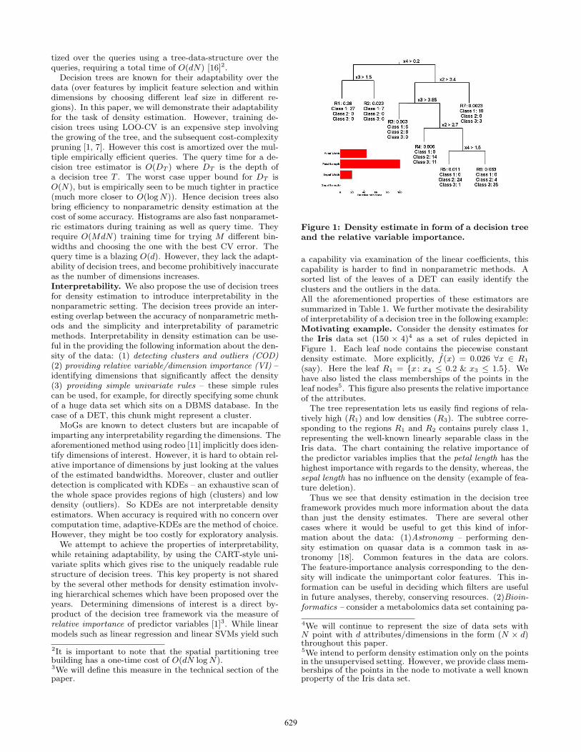
Figure 1: Density estimate in form of a decision treeand the relative variable importance.

a capability via examination of the linear coefficients, thiscapability is harder to find in nonparametric methods. Asorted list of the leaves of a DET can easily identify theclusters and the outliers in the data.All the aforementioned properties of these estimators aresummarized in Table 1. We further motivate the desirabilityof interpretability of a decision tree in the following example:Motivating example. Consider the density estimates forthe Iris data set (150 × 4)4 as a set of rules depicted inFigure 1. Each leaf node contains the piecewise constantdensity estimate. More explicitly, f(x) = 0.026 ∀x ∈ R1

(say). Here the leaf R1 = {x : x4 ≤ 0.2 & x3 ≤ 1.5}. Wehave also listed the class memberships of the points in theleaf nodes5. This figure also presents the relative importanceof the attributes.

The tree representation lets us easily find regions of rela-tively high (R1) and low densities (R3). The subtree corre-sponding to the regions R1 and R2 contains purely class 1,representing the well-known linearly separable class in theIris data. The chart containing the relative importance ofthe predictor variables implies that the petal length has thehighest importance with regards to the density, whereas, thesepal length has no influence on the density (example of fea-ture deletion).

Thus we see that density estimation in the decision treeframework provides much more information about the datathan just the density estimates. There are several othercases where it would be useful to get this kind of infor-mation about the data: (1)Astronomy – performing den-sity estimation on quasar data is a common task in as-tronomy [18]. Common features in the data are colors.The feature-importance analysis corresponding to the den-sity will indicate the unimportant color features. This in-formation can be useful in deciding which filters are usefulin future analyses, thereby, conserving resources. (2)Bioin-formatics – consider a metabolomics data set containing pa-

4We will continue to represent the size of data sets withN point with d attributes/dimensions in the form (N × d)throughout this paper.5We intend to perform density estimation only on the pointsin the unsupervised setting. However, we provide class mem-berships of the points in the node to motivate a well knownproperty of the Iris data set.

629

tient information with over 20000 features, where the taskis to differentiate cancer patients from healthy patients [19].Density estimation performed over all patients’ profiles canreveal which features are responsible for the main variationwithin, say, cancer patients, or within healthy patients. Thisis different from feature selection for classification whichwould select features which most differentiate the patientswith cancer from the rest. In addition, cluster and outlierdetection performed on this data set will produce interestingand possibly crucial information.

Moreover, a representative partition of the state space byitself sheds light on the underlying structure of the distri-bution. Such information is particularly valuable in highdimensional problems where direct visualization of the datais difficult.Remark. DETs are similar to variable bin-width histograms,but are restricted only to a hierarchical partitioning of thedata (hence possibly having lower accuracy than the bestpossible variable bin-width histogram, although our experi-ments suggest otherwise).

1.2 OverviewThe focus of this paper is to develop a rigorous decision-

tree-structured density estimator and demonstrate the use-fulness and interpretability of the same.

In Section 2, we discuss existing connections between den-sity estimation and decision trees. In the following section,we define an estimator based on the decision tree and ap-ply the decision-tree framework for density estimation usingthis estimator. We also provide certain asymptotic prop-erties of the decision-tree-structured estimator. Section 4contains experimental results displaying the performance ofDETs with some comparisons with histograms and KDEs.The adaptability of DETs is demonstrated by using somesynthetic data sets. High dimensional image data sets areused to demonstrate the DETs’ interpretability and theirapplication to classification. Training and querying time ofDETs are compared with the fastest training and queryingmethod for KDEs (KDE∗s). In the final section, conclusionsare discussed along with certain open questions.

2. FURTHER RELATED WORKDecision trees have been used alongside density estimation

in earlier works. For example, Kohavi, 1996 [20] and Smythet al., 1995 [21] use decision trees for the supervised task ofclassification, and density estimation (with naıve Bayes clas-sifiers and KDEs respectively) is used solely for the purposeof obtaining a smoother and more accurate classification andclass-conditional probabilities in contrast to the piecewiseconstant non-smooth estimates of the standard classificationtrees. Decision trees been used for the task of diagnosingextrapolation [22] by building a classification tree differen-tiating the given data set from a random sample from auniform distribution in the support of the data set. Thistree provides a way to compute a measure for extrapolation.This measure can be indirectly used to compute the density,but the tree still performs classification. Decision trees havealso been used in the supervised setting for estimating thejoint probability (of the data and the label of the trainingexamples) [23] for censored data by replacing the standardloss function (for example 0-1 loss or Gini-index) with thenegative loglikelihood of the joint density.

The idea of having a nested hierarchy of partitions of the

support of the data has been used for dicretization of univari-ate data [24]. The set of observations are partitioned on thebasis of the density using the loglikelihood loss function. Butthe focus is solely on univariate data. Decision trees havealso been used in an unsupervised setting to perform hierar-chical clustering [25] but do not trivially translate to densityestimation. Siedl et al., 2009 [26] propose a novel methodfor indexing the density model in the form of a tree (calledBayes tree) for fast access with desired level of accuracy.This tree is grown bottom-up from the estimate of a KDEfor the whole data set. The Bayes tree uses MoGs to indexthe density at the intermediate levels (increasing the numberof Gaussians with the depth). This tree successfully locatesclusters in the data. However, being a MoG, it fails to de-termine relative relevance of the dimensions. Polya trees[27] are hierarchical spatial partitioning trees but used as aprior for probability measures over the data space. Densityestimation is done either by computing the posterior meandensity given this prior or “learning” a fixed tree topologyand computing the piecewise constant estimate conditionalon this topology.

DETs are related in spirit, however, they will be learnedby directly minimizing the density estimation loss and theestimates are finally obtained directly from the tree. More-over, the aforementioned methods, though hierarchical innature, do not share the interpretability and feature selec-tion properties of decision trees, which are based on univari-ate splits.

3. DENSITY ESTIMATION TREEThis section provides the road map to perform density es-

timation using decision trees. We define an estimator andthe corresponding loss function to be minimized during thetraining of the decision tree for continuous and mixed data.Following that, we explain the process of learning the op-timal decision tree over the given sample and provide anasymptotic property of the DET.

3.1 Continuous Features

Definition 1. The piecewise constant density estimateof the decision tree T built on a set S of N observations inR

d is defined as

fN (x) =∑l ∈T

|l |NVl

I(x ∈ l ) (1)

where T is the set of leaves of the decision tree T repre-senting the partitions of the data space, |l | is the number ofobservations of S in the leaf l , Vl is the volume of the leafl within the d dimensional bounding box of S and I(·) is theindicator function.

A decision tree T requires a notion of a loss function R(T )which is minimized using a greedy algorithm to construct atree on the set of observations. For the unsupervised task ofdensity estimation, we consider the Integrated Squared Er-ror (ISE) loss function [10]. The ISE gives a notion of overalldistance between the estimated and the true density and isa favored choice in nonparametric density estimation for itsinherent robustness in comparison to maximum-likelihood-based loss functions [8]. However, other distance functionssuch as the KL-divergence can be used as the loss function.We will explore this in the longer version of the paper.

630

The task of learning a DET would involve solving thefollowing optimization problem:

minfN∈FN

∫X

(fN (x)− f(x)

)2dx (2)

where FN is the class of estimators of form in Definition 1that can learned with any set of N observations. After ex-panding the square and the following Monte-Carlo substi-tution

∫XfN (x)f(x)dx ≈ 1

N

∑Ni=1 fN (Xi) (where {Xi}Ni=1

is the training set), the objective function in Eq. 2 is re-placed by the following consistent plug-in estimator of theISE [10]6:

minfN∈FN

{∫X

(fN (x)

)2dx− 2

N

N∑i=1

fN (Xi)

}(3)

Using the piecewise constant estimator from Definition 1(which is constant within each leaf l ), the objective functionin Eq. 3 is replaced with the following:

∑l ∈T

{∫l

( |l |NVl

)2

dx− 2

N

|l |NVl

· |l |}

(4)

by substituting

f2N (x) =

∑l ∈T

( |l |NVl

)2

I(x ∈ l )

(since the cross terms in the expansion of f2N (x) vanish be-

cause of the indicator function) and simple calculation showsthat

N∑i=1

fN (Xi) =N∑i=1

∑l ∈T

|l |NVl

· I(Xi ∈ l ) =∑l ∈T

|l |NVl

· |l |

By making the following substitution∫l

( |l |NVl

)2

dx =

( |l |NVl

)2 ∫ldx =

( |l |NVl

)2

· Vl ,

the estimator of the ISE for DET has the following form:

∑l ∈T

{− |l |2N2Vl

}(5)

Defining Eq. 5 as the error R(T ) of the tree, the greedysurrogate of the error for any node t (internal or otherwise)can be defined as

R(t) = − |t |2N2Vt

. (6)

The tree is grown in a top down manner by maximizing thereduction in this greedy surrogate of the error over the givenobservations.

3.2 Mixed FeaturesFor density estimation over data with mixed features, we

define a novel density estimator and a loss function involvingordinal and categorical data along with continuous data thatcan be used to learn DETs with mixed data:

6The term∫X(f(x))2 dx is removed from the objective func-

tion since it is independent of the estimate and hence doesn’taffect the optimum.

Definition 2. Let S ⊂ Rd × Z

d′× C

d′′

with d real fea-

tures, d′ordinal features and d

′′categorical features. The

piecewise constant density estimator of the decision tree Tbuilt on S is defined as

fN (x) =∑l ∈T

|l | · I(x ∈ l )

N · Vld ·∏d′l

j=1 Rlj ·∏d′′l

i=1 Mli

(7)

where Vld is the volume of the leaf l within the d dimensionalbounding box of the real part of S, Rlj is the range of the

ordinal values in the jth of the d′l ordinal dimensions present

in l and Mli is the number of categories present in l for the

ith of the d′′l categorical dimensions present in l .

The error at a node t corresponding to the ISE is then ob-tained as

R(t) = − |t |2

N2 · Vtd ·∏d′t

j=1 Rtj ·∏d′′t

i=1 Mti

(8)

where Vtd is the volume of the node t in the d real dimen-sions, Rtj is the range of the ordinal values in the jth of the

d′t ordinal dimensions present in t and Mti is the number

of categories present in t for the ith of the d′′t categorical

dimensions present in t .

3.3 Tree ConstructionWe use the tree learning algorithm presented in Breiman,

et al.,1984 [1]. The splitting, pruning and the cross-validationprocedures are modified to work with this new loss functionand for the unsupervised task of density estimation.Splitting. For growing the tree, each node is split into twochildren. Let S be the set of all univariate splits.

Definition 3. [1] The best split s∗ of a node t is the splitin the set of splits S which maximally reduces R(T ).

This is done by greedily reducing R(t) for all the terminalnodes t of the current tree. Hence, for any currently terminalnode, we need to find a split s∗ for a node t into tL and tRsuch that

s∗ = argmaxs∈S

{R(t)−R(tL)−R(tR)} (9)

where |t | = |tL| + |tR|. For continuous and ordinal dimen-sions, this optimization is performed by trying every |t | − 1possible splits of the data in each of the dimensions. Forcategorical dimensions, the splits are performed in the man-ner similar to the CART model [1]. The splitting is stoppedwhen the node size |t | goes below a certain threshold (sayNmin).Pruning. To avoid overfitting, we use the minimal cost-complexity pruning [1]. The regularized error of a subtreerooted at a node t is defined as

Rα(t) = R(t) + α · |t | (10)

where α is a regularization parameter (to be estimated throughcross-validation) and t is the set of leaves in the subtreerooted at t . The value of α is gradually increased anda subtree rooted at t is pruned for the value of α whereRα(t) = Rα({t}), the regularized error of the pruned sub-tree. Since the size of the initial tree constructed by thesplitting algorithm described previously is finite, the num-ber of possible values of α at which a prune occurs is finite

631

and can be calculated efficiently. Hence we only need to se-lect the optimal α from a finite set of values (See Section 3.3in Breiman, et al., 1984 [1] for complete details).Cross-validation. The leave-one-out cross-validation(LOO-CV) estimator of the density estimation loss functionin Eq. 3 is given by

J(α) =

∫X

(fαN (x)

)2dx− 2

N

N∑i=1

fα(−i)(Xi) (11)

where fαN is the estimator with the decision tree T pruned

with a regularization parameter α, and fα(−i) is the estimator

with the decision tree T(−i) built without the training ex-ample Xi pruned with the regularization parameter α. ThisLOO-CV estimator is obtained from Silverman, 1986 [10] byswitching the regularization parameter (replacing the band-width with α). The best sized tree is the tree T pruned withthe parameter α∗ such that:

α∗ = argminα

J(α) (12)

3.4 Asymptotic PropertiesWe show that the method is nonparametric – it is con-

sistent under mild assumptions on the model class of theinput distribution f . Consistency is typically shown [28]

for a nonparametric estimator fN obtained from a set of Nobservations by showing that

Pr

(lim

N→∞

∫X

(fN (x)− f(x)

)2dx = 0

)= 1. (13)

We prove the consistency of DETs on data with continuousfeatures. The proof of consistency of the density estimatorproposed in Definition 1 follows arguments similar to thoseused to show the consistency of regression trees [1] .

Theorem 1. The estimator fN defined in Definition 1satisfies Eq. 13.

Proof. Given a fixed positive integer d1, let B denotethe collection of all sets t ⊂ X that can be described asthe solution set to a system of d1 inequalities, each of theform bTx ≤ c for b ∈ R

d and c ∈ R. Now in a decisiontree T , every leaf l ∈ T is the solution set of a system ofd1 inequalities of the form bTx ≤ c with b ∈ R

d with justone entry equal to 1 and the rest of the entries equal to 0.Therefore, T ⊂ B.

Let Xn, n ≥ 1, be a random sample from a density func-tion f on X. For N ≥ 1, let FN denote the empirical distri-bution of Xn, 1 ≤ n ≤ N , defined on a set t ⊂ X by

FN (t) =1

N

N∑n=1

I(Xn ∈ t) =|t|N

=

∫t

fN (x)dx (14)

where |t| is the number of random samples in the set t ∩{Xn}Nn=1 and fN (x) is the estimator given in Definition 1.

According to a general version of the Glivenko-Cantellitheorem [29],

Pr

(lim

N→∞supt∈B

|FN (t)−∫t

f(x)dx| = 0

)= 1. (15)

By Eq.14 and 15, we get

Pr

(lim

N→∞supt∈B

|∫t

fN (x)dx−∫t

f(x)dx| = 0

)= 1

⇒ Pr

(lim

N→∞supt∈B

∫t

|fN (x)− f(x)|dx ≥ 0

)= 1.

Assuming that limN→∞ Pr(diameter(t) ≥ ε) = 0, hencePr(limN→∞

∫tdx = 0

)= 1, we get the following with prob-

ability 1

limN→∞

supt∈B

∫t

|fN (x)− f(x)|dx ≤

limN→∞

|fN (x′)− f(x′)| ·∫t

dx for some x′ ∈ t = 0

This assumption is commonly used for the consistency ofdata-partitioning estimators [30] and is justified since asN → ∞, the diameter of any leaf node would become smallerand smaller since the leaf node can only have a boundednumber of points. Hence

Pr

(lim

N→∞supt∈B

∫t

|fN (x)− f(x)|dx = 0

)= 1

⇒ Pr

(lim

N→∞

∫X

(fN (x)− f(x)

)2dx = 0

)= 1.

Hence fN satisfies Eq. 13.

4. EXPERIMENTSIn this section, we demonstrate the performance of DETs

under different conditions using synthetic and real data sets.Estimation accuracies of DETs are compared with existingnonparametric estimators. We exhibit the interpretabilityof DETs with two real data sets. Furthermore, densityestimates of DETs are applied to classification and subse-quent labelling accuracies are presented. Finally, the speedof training and querying DETs are presented on several realdata sets and compared with an existing method. We onlyconsider continuous and ordinal data in this paper for thelack of space. Experiments with categorical and mixed datawill be presented in the longer version of the paper.

4.1 Estimation Accuracy: Synthetic ExamplesFor the unsupervised task of density estimation, estima-

tion accuracy can only be computed on synthetic data sets.We choose the best-sized tree through LOO-CV. To com-pute estimation error on synthetic data for density queries,we use 2 measures: Root Mean Squared Error (RMSE) andHellinger Distance (HD). We compare DETs only with othernonparametric density estimators since parametric estima-tors would involve choosing the model class (like choosingthe number of Gaussians in MoGs). We report the com-parison between DETs, histograms (bin-width selected byLOO-CV) and KDEs (using the Gaussian kernel) with thebandwidth selected by unbiased LOO-CV using the ISE cri-terion (FBW) and by local rodeo (local r-KDE) (VBW) onsynthetic data sets.Example 1. (Strongly skewed distribution in one dimen-sion) This distribution is defined as

X ∼7∑

i=0

1

8N(3

((2

3

)i

− 1

),

(2

3

)2i).

Figure 2 shows the estimated density functions by a DET,a histogram and two KDEs for a sample size N = 1000.Because of the high skewness of the density function, theKDE (FBW) and the histogram fail to fit the very smooth

632

−4 −3 −2 −1 0 1 2 3 40

0.2

0.4

0.6

0.8

1

1.2

1.4

x

dens

ity

DETTrue Density

(a) DET

−4 −3 −2 −1 0 1 2 3 40

0.2

0.4

0.6

0.8

1

1.2

1.4

x

dens

ity

HistogramTrue Density

(b) Histogram

−4 −3 −2 −1 0 1 2 3 40

0.2

0.4

0.6

0.8

1

1.2

1.4

x

dens

ity

KDETrue Density

(c) KDE (FBW)

−4 −3 −2 −1 0 1 2 3 40

0.2

0.4

0.6

0.8

1

1.2

1.4

x

dens

ity

RODEO−KDETrue Density

(d) local r-KDE

Figure 2: The density estimates obtained with 1000points for Example 1 using DET, Histogram andKDEs compared to the true density.

Table 2: Estimation errors for Histograms, KDEsand DETs with increasing number of observations

Type N Hist KDE(FBW) local r-KDE DET

RMSE102 0.2213 0.1748 0.1318 0.2548103 0.1158 0.0949 0.1339 0.1090104 0.0565 0.0235 0.0596 0.0527

HD102 0.1292 0.2365 0.0967 0.1187103 0.0832 0.0684 0.2343 0.0278104 0.01 0.0130 0.1634 0.0072

tail. The fixed bandwidth/binwidth results in a highly wig-gly estimate of the very smooth tail. The DET provides apiecewise constant estimate, but it adjusts to the differentparts of the density function by varying the leaf size – thetree has small leaves closer to the spike where the densityfunction changes rapidly, having larger leaves where the den-sity function does not change rapidly. This demonstrates theadaptability of DETs within the same dimension. The localr-KDE exhibits the same adaptability by obtaining differentbandwidths at different regions, hence capturing the smoothtail of the true density.

Table 2 provides the estimation errors with increasingsample sizes for the different methods. The RMSE valuesare fairly close and the HD values for the DETs are in factbetter than that of KDE using unbiased LOO-CV. This canbe attributed to the adaptive nature of DET with respectto the leaf sizes. The error values of local r-KDE are betterthan DET when the data set size is small (in case of largerdata sets, the local method might be overfitting over thisinstance of the data set). The accuracies of the histogramestimators and DETs are comparable in this univariate ex-ample. But we will demonstrate in the next example thatthe performance of histograms decline with increasing di-mensions.Example 2. (Two dimensional data – Mixture of Beta dis-tributions in one dimension, uniform in the other dimension)We create a (600 × 2) data set by sampling one dimensionas a mixture of Beta distributions and the other dimensionas a uniform distribution

X1 ∼ 2

3B(1, 2) + 1

3B(10, 10);X2 ∼ U(0, 1).

00.2

0.40.6

0.81 0

0.5

1

0

0.5

1

1.5

2

Irrelevant dimension

Relevant dimension

Den

sity

(a) DET (b) Histogram

00.2

0.40.6

0.81 0

0.5

1

0

0.5

1

1.5

2

2.5

3

Irrelevant dimRelevant dim

Den

sity

(c) KDE (FBW)

00.2

0.40.6

0.81 0

0.2

0.4

0.6

0.8

10

0.5

1

1.5

2

2.5

Irrelevant dimensionRelevant dimension

Den

sity

(d) local r-KDE

Figure 3: Perspective plots of the density estimatesfor a DET, a Histogram and two KDEs on the dataset in Example 2.

Figure 3 shows the 2-dimensional density estimates of aDET, a histogram and two KDEs. The DET fits the ir-relevant uniform dimension perfectly, while closely approxi-mating the mixture of Beta distributions in the relevant di-mension. The KDE with fixed bandwidth and the histogramestimator completely fail to fit the irrelevant dimension. Thelocal r-KDE does a better job of fitting the irrelevant dimen-sion compared to the KDE (FBW), but still does not entirelycapture the uniform density.

4.2 Interpretability: Variable ImportanceThe decision-tree framework defines a measure of rele-

vance for each of the predictor variables [1] as following:

Definition 4. The measure of relevance Id (T ) for eachattribute Xd (the d th attribute) in a decision tree T is definedas

Id (T ) =

|T |−1∑t=1

ι2t I(d(t) = d ) (16)

where the summation is over the |T | − 1 internal nodes ofthe tree T , and the attribute d(t) used to partition node tobtains ι2t improvement in squared error over the constantfit in node t .

We use this measure to present the interpretability of theDETs on two real data sets.Example 3. (Iris data set) We perform density estimationon this 4 dimensional data set and compute variable impor-tance for each of the dimensions. Figure 1 displays the treeand the relative variable importance. The interpretation hasbeen explained in Section 1.1.Example 4. (MNIST digits – image data) Each image has28-by-28 pixels providing a 784-dimensional data set. Weperform density estimation on the 5851 images of the digit8 (left panel of Figure 4). This is also an instance of per-forming density estimation with ordinal data since the pixelvalues are discrete. We compute the variable importance ofeach of the dimensions (pixels in this case). The right panelof Figure 4 displays the results obtained. The black pix-els indicate pixels with zero variable importance in density

633

(a) Originals (b) Variable Importance

Figure 4: Relative importance of the predictor vari-ables (pixels in this case) in density estimation forimages of digit 8.

Table 3: Classification Accuracy: r-KDE vs. DETCase # Train # Test r-KDE DET1v7 240 121 0.93 0.912v7 237 119 0.97 0.873v8 238 119 0.81 0.815v8 237 119 0.86 0.728v9 236 118 0.75 0.77All 1347 450 0.70 0.73

estimation. For the pixels with non-zero variable impor-tance, the color transitions for green (indicating low relativevariable importance) to red (indicating high relative vari-able importance). The marginal densities of many pixelsare close to point masses. Hence the density does not varyat all in those dimensions, and the relative variable impor-tance depicted in Figure 4 indicates that the DET is capableof capturing this property of the data.

4.3 ClassificationAs mentioned earlier, density estimation is a common sub-

routine in classification where the class-conditional densityp(x|C) is to be estimated for the query point x using the

training setX. The estimated class C(x) = argmaxC P (x|C)·P (C). We compare the accuracy of classification betweenthe density estimates computed by DETs and local r-KDEs.

Example 5. (Opt-digits – image data (1797 × 64) [31])We conduct binary as well as multi-class classification. Forbinary classification, we consider the following cases: 1 vs.7, 2 vs. 7, 3 vs. 8, 5 vs. 8, 8 vs. 9. We perform multi-class classification using all the classes (0-9). Table 3 liststhe classification accuracies for the different tasks. In mostcases, the accuracies are close for the two methods of den-sity estimation, with the r-KDEs being more accurate thanthe DETs. But in the last two cases, the DETs outperformthe r-KDEs. Moreover, the whole experiment (training andtesting) with the DETs is much faster than the one usingthe local r-KDEs. For example, in the last experiment per-forming multi-class classification required ∼ 8 seconds usingDETs and ∼ 500 seconds using r-KDEs7.

4.4 SpeedWe compare DETs to KDE∗s(FBW) using the fast ap-

proximate dual-tree algorithm [32] with kd-trees. We useLOO-CV to estimate the optimal bandwidth for the KDE∗s7The DET is implemented in C++ and the rodeo-KDE isimplemented using MATLAB on the same machine.

Table 4: Timings (in seconds) for training(T) andall queries(Q) with KDE∗s and DETsData set T(KDE∗) T(DET) Q(KDE∗) Q(DET)sj2 93.77 485.77 11.79 0.0026Colors 101.68 427.02 12.11 0.0022Bio 421.22 1213.84 5.7 0.0069Pall7 1240.75 1719.26 10.67 0.0046psf 18039.27 32456.43 77.48 0.975

sj2 colors bio pall7 psf10

0

101

102

103

104

Spe

edup

Speedups in query time

Figure 5: Query Time speedup for the DTE over theKDE. Note that the KDE is faster than the DTE incase of training.

(FBW). Real world data sets drawn from the SDSS reposi-tory [33] (SJ2 (50000× 2), PSF (3000000× 2)) and the UCIMachine Learning Repository [31] (Colors (50000 × 2), di-mension reduced version of the Bio dataset (100000 × 5),Pall7 (100000 × 7)) are used. The query set is same as thetraining set in all the experiments and the KDE∗s providethe leave-one-out estimates.

For the KDE∗, we use around H ≈ 10 bandwidths andchose the one with the best CV error. Usually, a muchlarger number of bandwidths are tried and the training timesscale linearly with H. For the DETs, we use 10-fold cross-validation since we were not able to find an efficient way toconduct LOO-CV with decision trees and it would requireprohibitively long time for these large data sets. This is onemajor limitation of this method. Howeover, for sufficientlylarge data sets, our experiments indicate that DETs trainedwith LOO-CV are only slightly more accurate than thosewith 10-fold CV.

The absolute timing values (in seconds) for training(T)and querying(Q) are given in Table 4. The speedups ofthe DETs over the KDE∗s in test/query time are shown inFigure 5. As can be seen from the results, the training timefor the decision tree algorithm is significantly larger thanthe LOO-CV for the KDE∗s, but the DETs provide up to3.5 orders of magnitude speedup in query time. The KDE∗sare fast to train, but their work comes at test time. Thisexperiment demonstrates the efficient querying of decisiontrees while also indicating that the task of training decisiontrees using LOO-CV is quite challenging.

5. DISCUSSION AND CONCLUSIONSThis framework of decision-tree-structured density esti-

mation provides a new way to estimate the density of a givenset of observations in the form of a simple set of rules whichare inherently intuitive and interpretable. This frameworkhas the capability of easily dealing with categorical, discreteas well as continuous variables and performs automatic fea-

634

ture selection. On having these rules, the density of a newtest point can be computed cheaply. All these features stemfrom the fact that the density estimation is performed in theform of a decision tree. Along with that, the DETs are eas-ily implementable like supervised decision trees. Althoughthese advantages come with the loss of accuracy, the DETsare shown to be consistent, and hence are quite reliable inthe presence of enough data.

Future directions of improvement include the reductionof the discontinuities in the density estimate because of thepiecewise constant estimator and the boundary bias sincethe DETs put no mass outside the span of the data. Bound-ary bias is a common problem for almost all density esti-mators. One possible remedy is to use a normalized KDEat each of the leaves instead of using the piecewise constantestimator (similar to the approach in Smyth et.al. [21].

An analysis of the convergence rate of the DETs wouldquantify the amount of loss of accuracy to account for thesimplicity of the estimator. Being effectively a variable bin-width histogram, we conjecture that the convergence rate forthe DETs would be o(N−2/3) for univariate data and betterthan histograms in higher dimensions since we demonstratethat the DETs can effectively model uninformative dimen-sions easily without requiring that extra number of pointsas imposed by the curse of dimensionality. Moreover, we areactively working on obtaining density dependent bounds onthe depth of the DETs to quantify the runtimes for trainingand test query.

Overall, this method for density estimation has immediateapplication to various fields of data analysis (for example,outlier and anomaly detection)8 and machine learning dueto its simple and interpretable solution to the fundamentaltask of density estimation.

6. REFERENCES[1] L. Breiman, J. H. Friedman, R. A. Olshen, and C. J. Stone.

Classification and Regression Trees. Wadsworth, 1984.[2] C. Bishop. Neural Networks for Pattern Recognition.

Oxford University Press, 1995.[3] C. M. Bishop. Pattern recognition and machine learning.

Springer, 2006.[4] R. O. Duda and P. E. Hart. Pattern Classification and

Scene Analysis. Wiley New York, 1973.[5] J. H. Friedman. A Recursive Partitioning Decision Rule for

Nonparametric Classification. Transactions on Computers,1977.

[6] J. H. Friedman. A tree-structured approach tononparametric multiple regression. Smoothing Techniquesfor Curve Estimation, 1979.

[7] T. Hastie, R. Tibshirani, and J. Friedman. The Elements ofStatistical Learning: Data Mining, Inference, andPrediction. Springer, 2001.

[8] L. Wasserman. All of Nonparametric Statistics.Physica-Verlag, 2006.

[9] C. Cortes and V. N. Vapnik. Support vector networks.Machine Learning, 1995.

[10] B. W. Silverman. Density Estimation for Statistics andData Analysis. Chapman & Hall/CRC, 1986.

[11] H. Liu, J. Lafferty, and L. Wasserman. SparseNonparametric Density Estimation in High DimensionsUsing the Rodeo. In AISTATS, 2007.

[12] P. Muller and F.A. Quintana. Nonparametric Bayesiandata analysis. Statistical Science, 2004.

8We will demonstrate these applications in the longer ver-sion of the paper.

[13] A. G. Gray and A. W. Moore. Nonparametric densityestimation: Toward computational tractability. In SIAMData Mining, 2003.

[14] D. Lee and A. G. Gray. Fast high-dimensional kernelsummations using the monte carlo multipole method. InAdvances in NIPS, 2008.

[15] A. Beygelzimer, S. Kakade, and J.C. Langford. Cover Treesfor Nearest Neighbor. ICML, 2006.

[16] P. Ram, D. Lee, W. March, and A. Gray. Linear-timealgorithms for pairwise statistical problems. In Advances inNIPS. 2009.

[17] J. Lafferty and L. Wasserman. Rodeo: SparseNonparametric Regression in High Dimensions. Arxivpreprint math.ST/0506342, 2005.

[18] R. Riegel, A. G. Gray, and G. Richards. Massive-ScaleKernel Discriminant Analysis: Mining for Quasars. InSIAM Data Mining (SDM), 2008.

[19] W. Guan, M. Zhou, C. Y. Hampton, B. B. Benigno, L. D.Walker, A. G. Gray, J. F. McDonald, and F. M. Fernandez.Ovarian Cancer Detection from Metabolomic LiquidChromatography/Mass Spectrometry Data by SupportVector Machines. BMC Bioinformatics Journal, 2009.

[20] R. Kohavi. Scaling up the accuracy of naive-Bayesclassifiers: A decision-tree hybrid. In KDD, 1996.

[21] P. Smyth, A. G. Gray, and U. M. Fayyad. Retrofittingdecision tree classifiers using kernel density estimation. InICML, 1995.

[22] G. Hooker. Diagnosing extrapolation: Tree-based densityestimation. In SIGKDD, 2004.

[23] A.M. Molinaro, S. Dudoit, and M.J. Van der Laan.Tree-based multivariate regression and density estimationwith right-censored data. Journal of Multivariate Analysis,2004.

[24] G. Schmidberger and E. Frank. Unsupervised discretizationusing tree-based density estimation. Lecture Notes inComputer Science, 2005.

[25] J. Basak and R. Krishnapuram. Interpretable hierarchicalclustering by constructing an unsupervised decision tree.IEEE transactions on knowledge and data engineering,2005.

[26] T. Seidl, I. Assent, P. Kranen, R. Krieger, andJ. Herrmann. Indexing density models for incrementallearning and anytime classification on data streams. InICEDT: Advances in Database Technology, 2009.

[27] W.H. Wong and L. Ma. Optional Polya tree and Bayesianinference. The Annals of Statistics, 2010.

[28] E. Parzen. On the estimation of a probability densityfunction and mode. Annals of Mathematical Statistics,pages 1065–1076, 1962.

[29] V. N. Vapnik and A. Y. Chervonenkis. On the uniformconvergence of relative frequencies of events to theirprobabilities. Theory of Probability and its Applications,1971.

[30] L. Devroye, L. Gyorfi, and G. Lugosi. A probabilistic theoryof pattern recognition. Springer Verlag, 1996.

[31] C.L. Blake and C.J. Merz. UCI repository of machinelearning databases. 1998.

[32] A. G. Gray and A. W. Moore. ‘n-body’ problems instatistical learning. In Advances in NIPS, 2000.

[33] R. Lupton, J.E. Gunn, Z. Ivezic, G.R. Knapp, S. Kent, andN. Yasuda. The SDSS Imaging Pipelines. Arxiv preprintastro-ph/0101420, 2001.

635