Articulated Pose Estimation using Discriminative Armlet Classifiers

Georgia Gkioxari1, Pablo Arbelaez1, Lubomir Bourdev2 and Jitendra Malik1

1University of California, Berkeley - Berkeley, CA 947202Facebook, 1601 Willow Rd, Menlo Park, CA 94025

{gkioxari,arbelaez,malik}@eecs.berkeley.edu,lubomir@fb.com

Figure 1. An example of an image where part detectors basedsolely on strong contours and edges will fail to detect the upperand lower parts of the arms.

Abstract

We propose a novel approach for human pose estimationin real-world cluttered scenes, and focus on the challengingproblem of predicting the pose of both arms for each per-son in the image. For this purpose, we build on the notionof poselets [4] and train highly discriminative classifiersto differentiate among arm configurations, which we callarmlets. We propose a rich representation which, in addi-tion to standard HOG features, integrates the information ofstrong contours, skin color and contextual cues in a princi-pled manner. Unlike existing methods, we evaluate our ap-proach on a large subset of images from the PASCAL VOCdetection dataset, where critical visual phenomena, suchas occlusion, truncation, multiple instances and clutter arethe norm. Our approach outperforms Yang and Ramanan[26], the state-of-the-art technique, with an improvementfrom 29.0% to 37.5% PCP accuracy on the arm keypointprediction task, on this new pose estimation dataset.

1. IntroductionSuppose our goal is to find the arms and hands of the

two gentlemen in Fig 1. We might aim to do so by fittinga stick figure model in one of its numerous manifestations[1, 7, 9, 19, 20] by detecting rectangles in the upper and

lower parts of the arms. But are there any contours there?It seems clear enough that how we detect the arm configu-rations of these people is from the position of the head andthe hands. And that information is enough to generate avery crisp prediction of the various joint locations.

This perspective, pose estimation as holistic recognition,can be found in papers from nearly a decade ago. Mori andMalik [16] matched whole body shapes of figures to ex-emplars using shape contexts and then transferred keypointlocations from exemplars to the test image. Shakhnarovichet al. [22] recovered the articulated pose of the human up-per body by defining parameter-sensitive hash functions toretrieve similar examples from the training set. Our posi-tion is that these approaches were philosophically correct,but their execution left much to be desired. The classi-fiers used were nearest neighbors and we have evidence thatdiscriminative classifiers such as support vector machines(SVMs) typically outdo nearest neighbor approaches [15].The features used were simple edges, and again over the lastdecade we have seen the superiority of descriptors basedon Histograms of Oriented Gradients (HOG) [5] in dealingwith clutter and capturing discriminative information whileavoiding early hard decisions.

We therefore revisit pose estimation as holistic recogni-tion using modern classifier and feature technology. Fig. 2presents an overview of our approach. During training, wepartition the space of keypoints and train models for armconfigurations, or armlets, using linear SVMs. Given a testimage, we apply the trained models and use the mean pre-dictions of the highest scoring activation to estimate the lo-cation of the joints. To train the armlets we extract featuresthat could capture the necessary cues for accurate arm key-point predictions. In Fig. 3 we show our choice of features.To capture the strong gradients in the image, we constructHOG features from local gradient contours [5] and gPb con-tours [2]. Another significant cue is the position, scale andorientation of the hands and of the rigid body parts, such ashead, torso and shoulders. We cannot assume that we haveperfect body part predictions. However, poselets [4] pro-vide a soft way of capturing the contextual information of

1

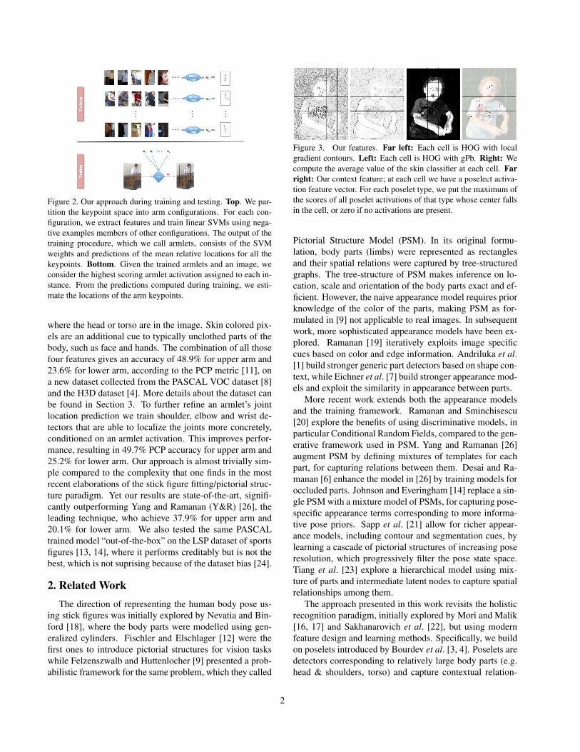
Figure 2. Our approach during training and testing. Top. We par-tition the keypoint space into arm configurations. For each con-figuration, we extract features and train linear SVMs using nega-tive examples members of other configurations. The output of thetraining procedure, which we call armlets, consists of the SVMweights and predictions of the mean relative locations for all thekeypoints. Bottom. Given the trained armlets and an image, weconsider the highest scoring armlet activation assigned to each in-stance. From the predictions computed during training, we esti-mate the locations of the arm keypoints.

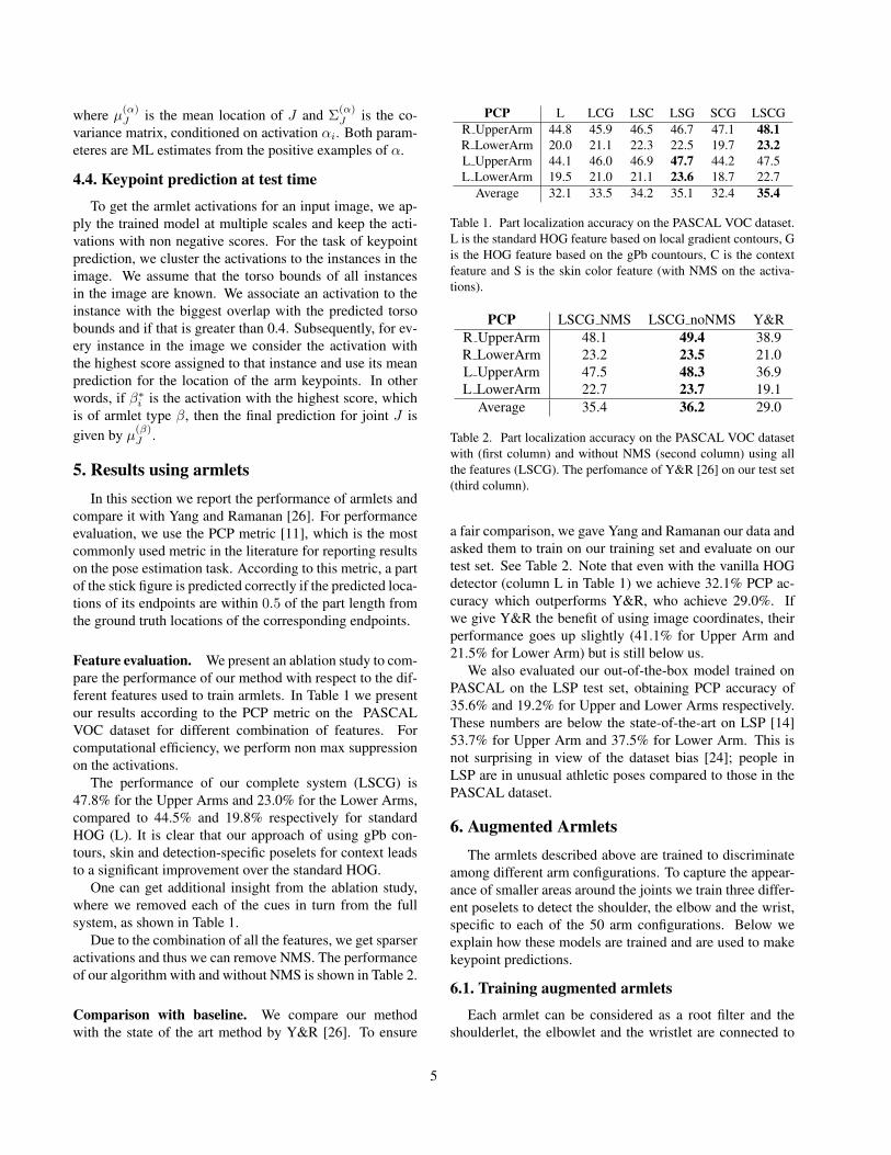
where the head or torso are in the image. Skin colored pix-els are an additional cue to typically unclothed parts of thebody, such as face and hands. The combination of all thosefour features gives an accuracy of 48.9% for upper arm and23.6% for lower arm, according to the PCP metric [11], ona new dataset collected from the PASCAL VOC dataset [8]and the H3D dataset [4]. More details about the dataset canbe found in Section 3. To further refine an armlet’s jointlocation prediction we train shoulder, elbow and wrist de-tectors that are able to localize the joints more concretely,conditioned on an armlet activation. This improves perfor-mance, resulting in 49.7% PCP accuracy for upper arm and25.2% for lower arm. Our approach is almost trivially sim-ple compared to the complexity that one finds in the mostrecent elaborations of the stick figure fitting/pictorial struc-ture paradigm. Yet our results are state-of-the-art, signifi-cantly outperforming Yang and Ramanan (Y&R) [26], theleading technique, who achieve 37.9% for upper arm and20.1% for lower arm. We also tested the same PASCALtrained model “out-of-the-box” on the LSP dataset of sportsfigures [13, 14], where it performs creditably but is not thebest, which is not suprising because of the dataset bias [24].

2. Related WorkThe direction of representing the human body pose us-

ing stick figures was initially explored by Nevatia and Bin-ford [18], where the body parts were modelled using gen-eralized cylinders. Fischler and Elschlager [12] were thefirst ones to introduce pictorial structures for vision taskswhile Felzenszwalb and Huttenlocher [9] presented a prob-abilistic framework for the same problem, which they called

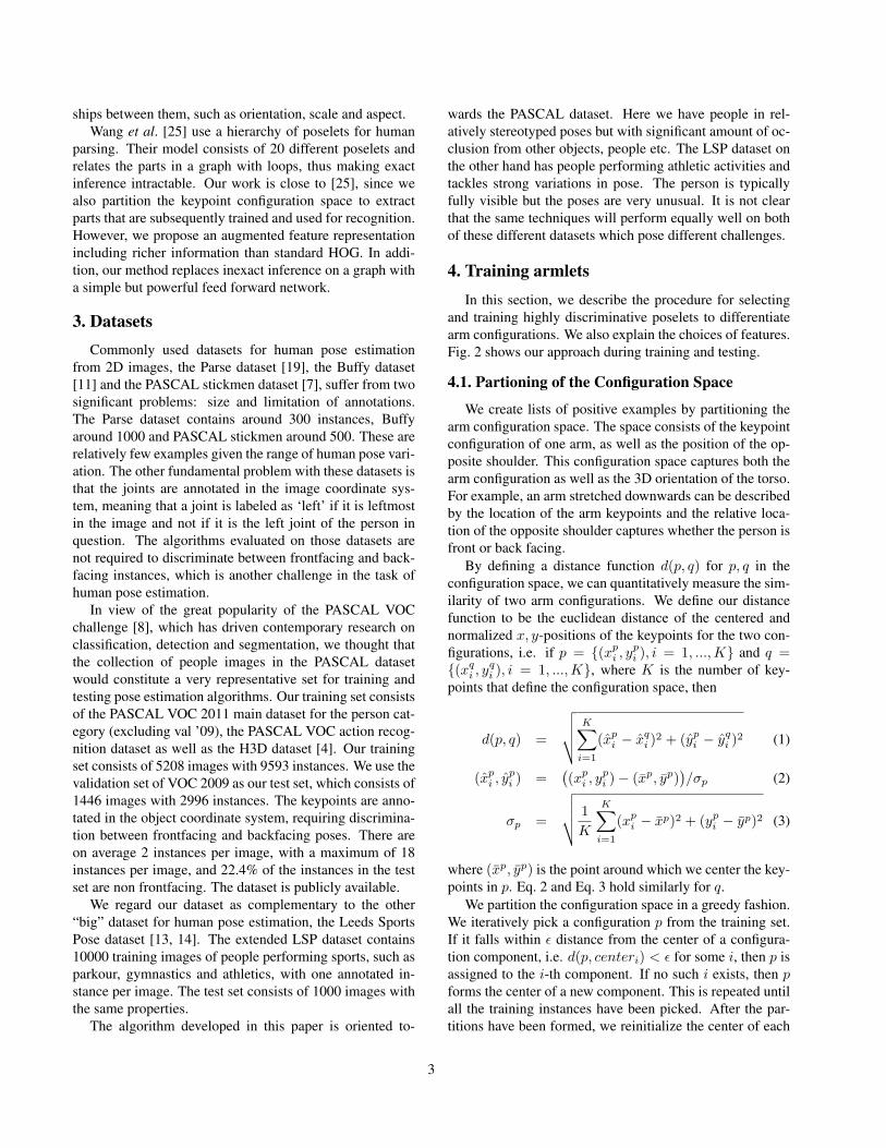
Figure 3. Our features. Far left: Each cell is HOG with localgradient contours. Left: Each cell is HOG with gPb. Right: Wecompute the average value of the skin classifier at each cell. Farright: Our context feature; at each cell we have a poselect activa-tion feature vector. For each poselet type, we put the maximum ofthe scores of all poselet activations of that type whose center fallsin the cell, or zero if no activations are present.

Pictorial Structure Model (PSM). In its original formu-lation, body parts (limbs) were represented as rectanglesand their spatial relations were captured by tree-structuredgraphs. The tree-structure of PSM makes inference on lo-cation, scale and orientation of the body parts exact and ef-ficient. However, the naive appearance model requires priorknowledge of the color of the parts, making PSM as for-mulated in [9] not applicable to real images. In subsequentwork, more sophisticated appearance models have been ex-plored. Ramanan [19] iteratively exploits image specificcues based on color and edge information. Andriluka et al.[1] build stronger generic part detectors based on shape con-text, while Eichner et al. [7] build stronger appearance mod-els and exploit the similarity in appearance between parts.

More recent work extends both the appearance modelsand the training framework. Ramanan and Sminchisescu[20] explore the benefits of using discriminative models, inparticular Conditional Random Fields, compared to the gen-erative framework used in PSM. Yang and Ramanan [26]augment PSM by defining mixtures of templates for eachpart, for capturing relations between them. Desai and Ra-manan [6] enhance the model in [26] by training models foroccluded parts. Johnson and Everingham [14] replace a sin-gle PSM with a mixture model of PSMs, for capturing pose-specific appearance terms corresponding to more informa-tive pose priors. Sapp et al. [21] allow for richer appear-ance models, including contour and segmentation cues, bylearning a cascade of pictorial structures of increasing poseresolution, which progressively filter the pose state space.Tiang et al. [23] explore a hierarchical model using mix-ture of parts and intermediate latent nodes to capture spatialrelationships among them.

The approach presented in this work revisits the holisticrecognition paradigm, initially explored by Mori and Malik[16, 17] and Sakhanarovich et al. [22], but using modernfeature design and learning methods. Specifically, we buildon poselets introduced by Bourdev et al. [3, 4]. Poselets aredetectors corresponding to relatively large body parts (e.g.head & shoulders, torso) and capture contextual relation-

2

ships between them, such as orientation, scale and aspect.Wang et al. [25] use a hierarchy of poselets for human

parsing. Their model consists of 20 different poselets andrelates the parts in a graph with loops, thus making exactinference intractable. Our work is close to [25], since wealso partition the keypoint configuration space to extractparts that are subsequently trained and used for recognition.However, we propose an augmented feature representationincluding richer information than standard HOG. In addi-tion, our method replaces inexact inference on a graph witha simple but powerful feed forward network.

3. DatasetsCommonly used datasets for human pose estimation

from 2D images, the Parse dataset [19], the Buffy dataset[11] and the PASCAL stickmen dataset [7], suffer from twosignificant problems: size and limitation of annotations.The Parse dataset contains around 300 instances, Buffyaround 1000 and PASCAL stickmen around 500. These arerelatively few examples given the range of human pose vari-ation. The other fundamental problem with these datasets isthat the joints are annotated in the image coordinate sys-tem, meaning that a joint is labeled as ‘left’ if it is leftmostin the image and not if it is the left joint of the person inquestion. The algorithms evaluated on those datasets arenot required to discriminate between frontfacing and back-facing instances, which is another challenge in the task ofhuman pose estimation.

In view of the great popularity of the PASCAL VOCchallenge [8], which has driven contemporary research onclassification, detection and segmentation, we thought thatthe collection of people images in the PASCAL datasetwould constitute a very representative set for training andtesting pose estimation algorithms. Our training set consistsof the PASCAL VOC 2011 main dataset for the person cat-egory (excluding val ’09), the PASCAL VOC action recog-nition dataset as well as the H3D dataset [4]. Our trainingset consists of 5208 images with 9593 instances. We use thevalidation set of VOC 2009 as our test set, which consists of1446 images with 2996 instances. The keypoints are anno-tated in the object coordinate system, requiring discrimina-tion between frontfacing and backfacing poses. There areon average 2 instances per image, with a maximum of 18instances per image, and 22.4% of the instances in the testset are non frontfacing. The dataset is publicly available.

We regard our dataset as complementary to the other“big” dataset for human pose estimation, the Leeds SportsPose dataset [13, 14]. The extended LSP dataset contains10000 training images of people performing sports, such asparkour, gymnastics and athletics, with one annotated in-stance per image. The test set consists of 1000 images withthe same properties.

The algorithm developed in this paper is oriented to-

wards the PASCAL dataset. Here we have people in rel-atively stereotyped poses but with significant amount of oc-clusion from other objects, people etc. The LSP dataset onthe other hand has people performing athletic activities andtackles strong variations in pose. The person is typicallyfully visible but the poses are very unusual. It is not clearthat the same techniques will perform equally well on bothof these different datasets which pose different challenges.

4. Training armletsIn this section, we describe the procedure for selecting

and training highly discriminative poselets to differentiatearm configurations. We also explain the choices of features.Fig. 2 shows our approach during training and testing.

4.1. Partioning of the Configuration Space

We create lists of positive examples by partitioning thearm configuration space. The space consists of the keypointconfiguration of one arm, as well as the position of the op-posite shoulder. This configuration space captures both thearm configuration as well as the 3D orientation of the torso.For example, an arm stretched downwards can be describedby the location of the arm keypoints and the relative loca-tion of the opposite shoulder captures whether the person isfront or back facing.

By defining a distance function d(p, q) for p, q in theconfiguration space, we can quantitatively measure the sim-ilarity of two arm configurations. We define our distancefunction to be the euclidean distance of the centered andnormalized x, y-positions of the keypoints for the two con-figurations, i.e. if p = {(xpi , y

pi ), i = 1, ...,K} and q =

{(xqi , yqi ), i = 1, ...,K}, where K is the number of key-

points that define the configuration space, then

d(p, q) =

√√√√ K∑i=1

(xpi − xqi )

2 + (ypi − yqi )

2 (1)

(xpi , ypi ) =

((xpi , y

pi )− (xp, yp)

)/σp (2)

σp =

√√√√ 1

K

K∑i=1

(xpi − xp)2 + (ypi − yp)2 (3)

where (xp, yp) is the point around which we center the key-points in p. Eq. 2 and Eq. 3 hold similarly for q.

We partition the configuration space in a greedy fashion.We iteratively pick a configuration p from the training set.If it falls within ε distance from the center of a configura-tion component, i.e. d(p, centeri) < ε for some i, then p isassigned to the i-th component. If no such i exists, then pforms the center of a new component. This is repeated untilall the training instances have been picked. After the par-titions have been formed, we reinitialize the center of each

3

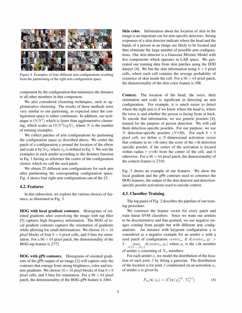
Figure 4. Examples of four different arm configurations resultingfrom the partitioning of the right arm configuration space.

component by the configuration that minimizes the distanceto all other members in that component.

We also considered clustering techniques, such as ag-glomerative clustering. The results of those methods werevery similar to our partioning, as expected since the con-figuration space is rather continuous. In addition, our tech-nique is O(N2) which is faster than agglomerative cluster-ing, which scales as O(N2logN), where N is the numberof training examples.

We collect patches of arm configurations by partioningthe configuration space as described above. We center thepatch of a configuration p around the location of the elbowand scale it by 2σp, where σp is defined in Eq. 3. We sort theexamples in each armlet according to the distance functionin Eq. 1 having as reference the center of the configurationcluster, which we call the seed patch.

We obtain 25 different arm configurations for each armafter partitioning the corresponding configuration space.Fig. 4 shows four right arm configurations out of the 25.

4.2. Features

In this subsection, we explore the various choices of fea-tures, as illustrated in Fig. 3.

HOG with local gradient contours. Histograms of ori-ented gradients after convolving the image with tap filter[5] captures high frequency information. The HOG of lo-cal gradient contours captures the orientation of gradientswhile allowing for small deformations. We choose 16× 16pixel blocks of four 8 × 8 pixel cells, and 9 bins for orien-tation. For a 96 × 64 pixel patch, the dimensionality of theHOG-tap feature is 2772.

HOG with gPb contours. Histograms of oriented gradi-ents of the gPb output of an image [2] will capture only thecontours that emerge from strong brightness, color and tex-ture gradients. We choose 16×16 pixel blocks of four 8×8pixel cells, and 8 bins for orientation. For a 96 × 64 pixelpatch, the dimensionality of the HOG-gPb feature is 2464.

Skin color. Information about the location of skin in theimage is an important cue for arm-specific detectors. Strongresponses of a skin detector indicate where the head and thehands of a person in an image are likely to be located andthus eliminate the large number of possible arm configura-tions. Our skin detector is a Gaussian Mixture Model withfive components which operates in LAB space. We gen-erated our training data from skin patches using the H3Ddataset [4]. We bin the skin information using 8 × 8 pixelcells, where each cell contains the average probability ofexistence of skin inside the cell. For a 96× 64 pixel patch,the dimensionality of the skin color feature is 308.

Context. The location of the head, the torso, theirorientation and scale is significant in detecting an armconfiguration. For example, it is much easier to detectwhere the right arm is if we know where the head is, wherethe torso is and whether the person is facing front or back.To encode that information, we use generic poselets [4],trained for the purpose of person detection. We will callthem detection-specific poselets. For our purpose, we useN detection-specific poselets (N=30). For each 8 × 8pixel cell, we define a N -dimensional activation vectorthat contains in its i-th entry the score of the i-th detectionspecific poselet, if the center of the activation is locatedwithin radius r (r=8) from the center of the cell, and 0otherwise. For a 96× 64 pixel patch, the dimensionality ofthe context feature is 2310.

Fig. 3 shows an example of our features. We show thelocal gradient and the gPb contours used to construct theHOG features, the output of the skin detector and detection-specific poselet activations used to encode context.

4.3. Classifier Training

The top panel of Fig. 2 describes the pipeline of our train-ing procedure.

We construct the feature vector for every patch andtrain linear SVM classifiers. Since we want our armletsto be discriminative and fine-grained, we use negative im-ages coming from people but with different arm config-urations. An instance with keypoint configuration q isconsidered as a negative example for an armlet α with aseed patch of configuration centerα, if d(centerα, q) >2 · max

i∈{1,...,Nα}d(centerα, pi) where pi is the i-th member

of armlet α consisting of Nα members.For each armlet α, we model the distribution of the loca-

tion of each joint J by fitting a gaussian. The distributionof the location x for joint J conditioned on an activation αiof armlet α is given by

Pm(x| αi) = N(x |µ(α)

J , Σ(α)J

)(4)

4

where µ(α)J is the mean location of J and Σ

(α)J is the co-

variance matrix, conditioned on activation αi. Both param-eteres are ML estimates from the positive examples of α.

4.4. Keypoint prediction at test time

To get the armlet activations for an input image, we ap-ply the trained model at multiple scales and keep the acti-vations with non negative scores. For the task of keypointprediction, we cluster the activations to the instances in theimage. We assume that the torso bounds of all instancesin the image are known. We associate an activation to theinstance with the biggest overlap with the predicted torsobounds and if that is greater than 0.4. Subsequently, for ev-ery instance in the image we consider the activation withthe highest score assigned to that instance and use its meanprediction for the location of the arm keypoints. In otherwords, if β∗i is the activation with the highest score, whichis of armlet type β, then the final prediction for joint J isgiven by µ(β)

J .

5. Results using armletsIn this section we report the performance of armlets and

compare it with Yang and Ramanan [26]. For performanceevaluation, we use the PCP metric [11], which is the mostcommonly used metric in the literature for reporting resultson the pose estimation task. According to this metric, a partof the stick figure is predicted correctly if the predicted loca-tions of its endpoints are within 0.5 of the part length fromthe ground truth locations of the corresponding endpoints.

Feature evaluation. We present an ablation study to com-pare the performance of our method with respect to the dif-ferent features used to train armlets. In Table 1 we presentour results according to the PCP metric on the PASCALVOC dataset for different combination of features. Forcomputational efficiency, we perform non max suppressionon the activations.

The performance of our complete system (LSCG) is47.8% for the Upper Arms and 23.0% for the Lower Arms,compared to 44.5% and 19.8% respectively for standardHOG (L). It is clear that our approach of using gPb con-tours, skin and detection-specific poselets for context leadsto a significant improvement over the standard HOG.

One can get additional insight from the ablation study,where we removed each of the cues in turn from the fullsystem, as shown in Table 1.

Due to the combination of all the features, we get sparseractivations and thus we can remove NMS. The performanceof our algorithm with and without NMS is shown in Table 2.

Comparison with baseline. We compare our methodwith the state of the art method by Y&R [26]. To ensure

PCP L LCG LSC LSG SCG LSCGR UpperArm 44.8 45.9 46.5 46.7 47.1 48.1R LowerArm 20.0 21.1 22.3 22.5 19.7 23.2L UpperArm 44.1 46.0 46.9 47.7 44.2 47.5L LowerArm 19.5 21.0 21.1 23.6 18.7 22.7

Average 32.1 33.5 34.2 35.1 32.4 35.4

Table 1. Part localization accuracy on the PASCAL VOC dataset.L is the standard HOG feature based on local gradient contours, Gis the HOG feature based on the gPb countours, C is the contextfeature and S is the skin color feature (with NMS on the activa-tions).

PCP LSCG NMS LSCG noNMS Y&RR UpperArm 48.1 49.4 38.9R LowerArm 23.2 23.5 21.0L UpperArm 47.5 48.3 36.9L LowerArm 22.7 23.7 19.1

Average 35.4 36.2 29.0

Table 2. Part localization accuracy on the PASCAL VOC datasetwith (first column) and without NMS (second column) using allthe features (LSCG). The perfomance of Y&R [26] on our test set(third column).

a fair comparison, we gave Yang and Ramanan our data andasked them to train on our training set and evaluate on ourtest set. See Table 2. Note that even with the vanilla HOGdetector (column L in Table 1) we achieve 32.1% PCP ac-curacy which outperforms Y&R, who achieve 29.0%. Ifwe give Y&R the benefit of using image coordinates, theirperformance goes up slightly (41.1% for Upper Arm and21.5% for Lower Arm) but is still below us.

We also evaluated our out-of-the-box model trained onPASCAL on the LSP test set, obtaining PCP accuracy of35.6% and 19.2% for Upper and Lower Arms respectively.These numbers are below the state-of-the-art on LSP [14]53.7% for Upper Arm and 37.5% for Lower Arm. This isnot surprising in view of the dataset bias [24]; people inLSP are in unusual athletic poses compared to those in thePASCAL dataset.

6. Augmented ArmletsThe armlets described above are trained to discriminate

among different arm configurations. To capture the appear-ance of smaller areas around the joints we train three differ-ent poselets to detect the shoulder, the elbow and the wrist,specific to each of the 50 arm configurations. Below weexplain how these models are trained and are used to makekeypoint predictions.

6.1. Training augmented armlets

Each armlet can be considered as a root filter and theshoulderlet, the elbowlet and the wristlet are connected to

5

Figure 5. HOG templates for the shoulderlet, the elbowlet and thewristlet for armlet 3 superimposed on a positive example of thatarmlet.

the root forming a star model (tree of depth one), similarto [10]. However, the position of the corresponding jointsw.r.t. the armlet activation is observed, in contrast to [10]where the location of the parts is treated as a latent variable.

We extract rectangular patches from the positive exam-ples of each armlet type. The patches are centered at thekeypoint of interest and at double the scale of the originalpositive example. Since the patches come from similar armconfigurations, defined by the armlet type, they are aligned,allowing for the use of rigid features such as HOG.

Each patch is described by a local gradient HOG descrip-tor as well as the skin color signal. The patches are 64× 64pixels and we use 16×16 pixel blocks of 8×8 pixel cells forboth features which are constructed as in Section 4.2. Weuse instance specific skin color models, which are GMMswith 5 components fitted on the LAB pixel values corre-sponding to the predicted face region of each instance asdictated by the detection specific poselet activations.

Subsequently, we learn a linear SVM using as negatives64 × 64 sized patches coming from the positive armlet ex-amples but not centered close to the joint in reference. Af-ter the first round of training, we re-estimate the positivepatches by running the detector in a small neighborhoodaround the original keypoint location. This allows for somesmall variations in the alignment of the examples comingfrom the armlet clustering and results in a better alignmentof the actual parts to be trained. A new model is trainedwith the improved positive examples. Fig. 5 shows an ex-ample of an armlet along with the HOG templates for theshoulderlet, the elbowlet and the wristlet.

6.2. Augmented armlet activations

We can use the activations of the shoulderlet, the el-bowlet and the wristlet to rescore the original armlet acti-vations. Strong part activations might indicate that the rightarmlet has indeed fired while weak part activations indicatea false positive activation.

Recall that for each armlet α, we computed the meanrelative location and the standard deviation of the three arm

keypoints from the positive examples of that armlet. Givenan activation of that particular armlet, these locations give arough estimate of where the joints might be located withinthe bounding box of the activation. We define an area ofinterest for each keypoint centered at the mean location andextending twice the empirical standard deviation. For eachpart, we detect its activations within the area of interest andrecord the highest scoring activation. In other words, eacharmlet activation αi is now described by its original detec-tion score sαi as well as the three maximum part activa-tion scores s(J)αi , J = 1, 2, 3 corresponding to the three armkeypoints. Let us call vαi the part activation vector whichcontains those four scores of the armlet activation αi.

For each armlet α, we can train a linear SVM wα withpositives Pα = {vαi | i ∈ TP (α)} where TP (α) is theset of true positive activations of armlet α and negativesNα = {vαi | i ∈ FP (α)} where FP (α) is the set of falsepositive activations of armlet α. An armlet activation αi hassubsequently an activation score σ

(wTαvαi

), where σ(·) is

a logistic function trained for each armlet α.

6.3. Using the augmented armlets for keypoint pre-dictions

The activations of the shoulderlets, the elbowlets and thewristlets can also be used for improved predictions of thelocation of the corresponding joints.

Assume α is an armlet and αi is the i-th activation of thatarmlet in an image I . The prior probability that joint J islocated at x is given by Eq. 4.

The score of a part activation at location x of the trainedmodel for joint J , after fitting a logistic on the SVM scores,can be interpreted as the confidence of the part model at thatlocation. In other words, if LJ is a binary random variable.indicating whether joint J is present, then the probability ofjoint J being present at location x

P(LJ | I, αi,x

)=

1

1 + exp(−γJαs(J)αi − δJα)

(5)

where {γJα , δJα} are the trained parameters of the logisticand s(J)αi the SVM score of the part model for joint J at x.

The predicted location of part J conditioned on the acti-vation αi is given by

x∗(J) = arg maxx

Pm(x| αi) · P(LJ | I, αi,x

)(6)

7. Results using augmented armletsWe can use the shoulderlets, elbowlet and wristlet trained

for each armlet to rescore the activations on the test setas well as make keypoint predictions, as described in Sec-tion 6. Table 3 shows the performance on the test set. Thefirst column shows the performance after picking the high-est scoring armlet activation, as described in Section 5. The

6

PCP LSCG LSCG augmented LSCG posteriorR UpperArm 49.4 50.2 50.2R LowerArm 23.5 23.4 25.0L UpperArm 48.3 49.3 49.2L LowerArm 23.7 24.5 25.4

Average 36.2 36.9 37.5

Table 3. Part localization accuracy on the PASCAL VOC datasetusing all the features (LSCG) using the mean relative location forjoint predictions of the highest scoring armlet activations (first col-umn), using the mean relative location for joint predictions of thehighest scoring augmented armlet activations (second column) andusing the posterior probability for joint predictions in Eq. 6 (thirdcolumn)

Figure 6. PCP localization accuracy for different values of thethreshold in the metric. The red curves show our performance forthe Upper and Lower Arm (mean across right and left). The bluecurves show the performance of [26]. (best viewed in color)

second column shows the performance after picking themaximum scoring activation of the augmented armlets tomake predictions for the joints using the mean relative loca-tions. The third column shows the performance after usingthe highest scoring activation of the augmented armlets tomake a prediction using the posterior probability (Eq 6). 1

Fig. 6 shows the PCP localization accuracy of our finalmodel compared to Yang and Ramanan [26] for differentthresholds for the PCP metric evaluation.

Fig. 7, 8 show examples of correct right and left, respec-tively, arm keypoint predictions. The bounds of the instancein question are shown in green. The red stick corresponds tothe upper arm and the blue to the lower arm of that instance.

Fig. 9 shows incorrect keypoint predictions for the rightand left arm corresponding to the instance highlighted ingreen.

8. DiscussionWe propose a straightforward yet effective framework

for training arm specific poselets for the task of joint po-sition estimation and we show experimentally that it givessuperior results on a challenging dataset.

1We also cross-checked by using bounding boxes rather than torsos todetermine the ground truth person, and the numbers change only slightlyto 47.5% for Upper and 23.8% for Lower Arms

Figure 7. Examples of correct right arm keypoint predictions. Redcorresponds to the upper arm and blue to the lower arm of theperson highlighted in green. (best viewed in color)

Figure 8. Examples of correct left arm keypoint predictions. Redcorresponds to the upper arm and blue to the lower arm of theperson highlighted in green. (best viewed in color)

Figure 9. Examples of incorrect keypoint predictions for the rightarm (top) and left arm (bottom) . Red corresponds to the upperarm and blue to the lower arm of the person highlighted in green.(best viewed in color)

The shortage of data for developing efficient human poseestimation algorithms has a significant impact on the perfor-mance for both our and Yang and Ramanan’s approach. Ourknowledge of the ground truth configuration on the test setenables us to cluster each test instance to one of the armlets.Thus, we can compute the PCP accuracy per armlet type

7

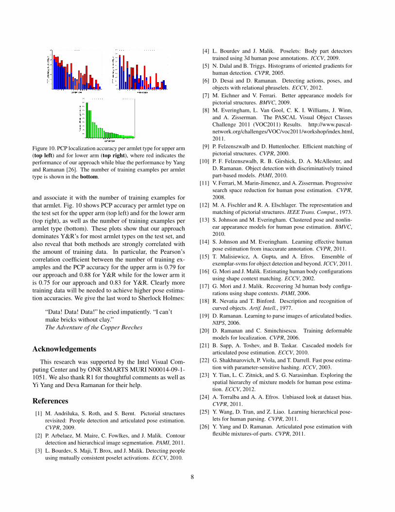
Figure 10. PCP localization accuracy per armlet type for upper arm(top left) and for lower arm (top right), where red indicates theperformance of our approach while blue the performance by Yangand Ramanan [26]. The number of training examples per armlettype is shown in the bottom.

and associate it with the number of training examples forthat armlet. Fig. 10 shows PCP accuracy per armlet type onthe test set for the upper arm (top left) and for the lower arm(top right), as well as the number of training examples perarmlet type (bottom). These plots show that our approachdominates Y&R’s for most armlet types on the test set, andalso reveal that both methods are strongly correlated withthe amount of training data. In particular, the Pearson’scorrelation coefficient between the number of training ex-amples and the PCP accuracy for the upper arm is 0.79 forour approach and 0.88 for Y&R while for the lower arm itis 0.75 for our approach and 0.83 for Y&R. Clearly moretraining data will be needed to achieve higher pose estima-tion accuracies. We give the last word to Sherlock Holmes:

“Data! Data! Data!” he cried impatiently. “I can’tmake bricks without clay.”The Adventure of the Copper Beeches

AcknowledgementsThis research was supported by the Intel Visual Com-

puting Center and by ONR SMARTS MURI N00014-09-1-1051. We also thank R1 for thoughtful comments as well asYi Yang and Deva Ramanan for their help.

References[1] M. Andriluka, S. Roth, and S. Bernt. Pictorial structures

revisited: People detection and articulated pose estimation.CVPR, 2009.

[2] P. Arbelaez, M. Maire, C. Fowlkes, and J. Malik. Contourdetection and hierarchical image segmentation. PAMI, 2011.

[3] L. Bourdev, S. Maji, T. Brox, and J. Malik. Detecting peopleusing mutually consistent poselet activations. ECCV, 2010.

[4] L. Bourdev and J. Malik. Poselets: Body part detectorstrained using 3d human pose annotations. ICCV, 2009.

[5] N. Dalal and B. Triggs. Histograms of oriented gradients forhuman detection. CVPR, 2005.

[6] D. Desai and D. Ramanan. Detecting actions, poses, andobjects with relational phraselets. ECCV, 2012.

[7] M. Eichner and V. Ferrari. Better appearance models forpictorial structures. BMVC, 2009.

[8] M. Everingham, L. Van Gool, C. K. I. Williams, J. Winn,and A. Zisserman. The PASCAL Visual Object ClassesChallenge 2011 (VOC2011) Results. http://www.pascal-network.org/challenges/VOC/voc2011/workshop/index.html,2011.

[9] P. Felzenszwalb and D. Huttenlocher. Efficient matching ofpictorial structures. CVPR, 2000.

[10] P. F. Felzenszwalb, R. B. Girshick, D. A. McAllester, andD. Ramanan. Object detection with discriminatively trainedpart-based models. PAMI, 2010.

[11] V. Ferrari, M. Marin-Jimenez, and A. Zisserman. Progressivesearch space reduction for human pose estimation. CVPR,2008.

[12] M. A. Fischler and R. A. Elschlager. The representation andmatching of pictorial structures. IEEE Trans. Comput., 1973.

[13] S. Johnson and M. Everingham. Clustered pose and nonlin-ear appearance models for human pose estimation. BMVC,2010.

[14] S. Johnson and M. Everingham. Learning effective humanpose estimation from inaccurate annotation. CVPR, 2011.

[15] T. Malisiewicz, A. Gupta, and A. Efros. Ensemble ofexemplar-svms for object detection and beyond. ICCV, 2011.

[16] G. Mori and J. Malik. Estimating human body configurationsusing shape context matching. ECCV, 2002.

[17] G. Mori and J. Malik. Recovering 3d human body configu-rations using shape contexts. PAMI, 2006.

[18] R. Nevatia and T. Binford. Description and recognition ofcurved objects. Artif. Intell., 1977.

[19] D. Ramanan. Learning to parse images of articulated bodies.NIPS, 2006.

[20] D. Ramanan and C. Sminchisescu. Training deformablemodels for localization. CVPR, 2006.

[21] B. Sapp, A. Toshev, and B. Taskar. Cascaded models forarticulated pose estimation. ECCV, 2010.

[22] G. Shakhnarovich, P. Viola, and T. Darrell. Fast pose estima-tion with parameter-sensitive hashing. ICCV, 2003.

[23] Y. Tian, L. C. Zitnick, and S. G. Narasimhan. Exploring thespatial hierarchy of mixture models for human pose estima-tion. ECCV, 2012.

[24] A. Torralba and A. A. Efros. Unbiased look at dataset bias.CVPR, 2011.

[25] Y. Wang, D. Tran, and Z. Liao. Learning hierarchical pose-lets for human parsing. CVPR, 2011.

[26] Y. Yang and D. Ramanan. Articulated pose estimation withflexible mixtures-of-parts. CVPR, 2011.

8