Density-equalizing map projections: Di usion-based …mejn/papers/geocomp.pdf · Density-equalizing...
23
Density-equalizing map projections: Diffusion-based algorithm and applications Michael T. Gastner and M. E. J. Newman Physics Department and Center for the Study of Complex Systems,, University of Michigan, Ann Arbor, MI 48109 Abstract Map makers have for many years searched for a way to construct cartograms—maps in which the sizes of geographic regions such as coun- tries or provinces appear in proportion to their population or some sim- ilar property. Such maps are invaluable for the representation of census results, election returns, disease incidence, and many other kinds of hu- man data. Unfortunately, in order to scale regions and still have them fit together, one is normally forced to distort the regions’ shapes, po- tentially resulting in maps that are difficult to read. Here we present a technique for making cartograms based on ideas borrowed from elemen- tary physics that is conceptually simple and produces easily readable maps. We illustrate the method with applications to disease and homi- cide cases, energy consumption and production in the United States, and the geographical distribution of stories appearing in the news. 1
Transcript of Density-equalizing map projections: Di usion-based …mejn/papers/geocomp.pdf · Density-equalizing...

Density-equalizing map projections:
Diffusion-based algorithm and applications
Michael T. Gastner and M. E. J. Newman
Physics Department and Center for the Study of Complex Systems,,
University of Michigan, Ann Arbor, MI 48109
Abstract
Map makers have for many years searched for a way to construct
cartograms—maps in which the sizes of geographic regions such as coun-
tries or provinces appear in proportion to their population or some sim-
ilar property. Such maps are invaluable for the representation of census
results, election returns, disease incidence, and many other kinds of hu-
man data. Unfortunately, in order to scale regions and still have them
fit together, one is normally forced to distort the regions’ shapes, po-
tentially resulting in maps that are difficult to read. Here we present a
technique for making cartograms based on ideas borrowed from elemen-
tary physics that is conceptually simple and produces easily readable
maps. We illustrate the method with applications to disease and homi-
cide cases, energy consumption and production in the United States,
and the geographical distribution of stories appearing in the news.
1

2 Michael T. Gastner and M. E. J. Newman
1 Introduction
Suppose we wish to represent on a map some data concerning, to take the
most common example, the human population. For instance, we might wish
to show votes in an election, incidence of a disease, number of cars, televisions,
or phones in use, numbers of people falling in one group or another of the
population, by age or income, or any other variable of statistical, medical,
or demographic interest. The typical course under such circumstances would
be to choose one of the standard (near-)equal-area projections for the region
of interest and plot the data on it either as individual data points or using
some sort of color code. The interpretation of such maps however can be
problematic. A plot of disease cases, for instance, will inevitably show high
incidence in cities and low incidence in rural areas, solely because there is
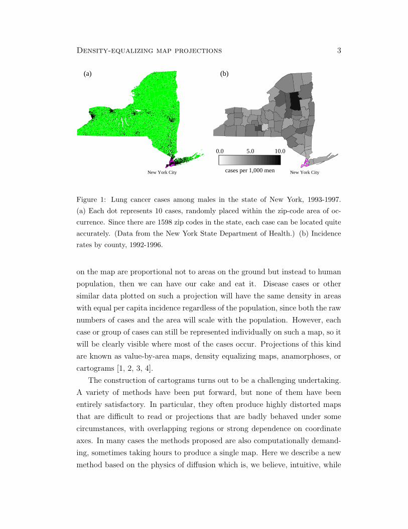
a higher density of people living in cities. Figure 1(a), for example, shows
the distribution of lung cancer cases among males in the state of New York
between 1993 and 1997. Cases are particularly dense in New York City and
its suburbs and sparse in the rural north of the state, but this could be purely
a population effect and nothing to do with the disease itself.
To get a clearer impression of the situation we can instead plot a fractional
measure of disease incidence rather than raw incidence data; we plot some
measure of the number of cases per capita, binned in segments small enough
to give good spatial resolution but large enough to give reliable sampling. Then
we can use a color code to indicate different per capita rates on the map, as
in Fig. 1(b). This procedure however has its own problems since it discards
all information about where most of the cases are occurring. In Fig. 1(b), for
example, there is now no way to tell that a large fraction of all cases occur in
the New York City area.
Ideally, we would like some geographic representation of the data that
allows us to see simultaneously where each individual case occurs as well as
the per capita incidence. Though it appears at first that these two goals are
irreconcilable, this is not in fact the case. On a normal area-preserving or
approximately area-preserving projection, such as that used in Fig. (1), they
are indeed irreconcilable. But if we can construct a projection in which areas
Density-equalizing map projections 3
0.0 5.0 10.0
cases per 1,000 menNew York City
(b)
New York City
(a)
Figure 1: Lung cancer cases among males in the state of New York, 1993-1997.
(a) Each dot represents 10 cases, randomly placed within the zip-code area of oc-
currence. Since there are 1598 zip codes in the state, each case can be located quite
accurately. (Data from the New York State Department of Health.) (b) Incidence
rates by county, 1992-1996.
on the map are proportional not to areas on the ground but instead to human
population, then we can have our cake and eat it. Disease cases or other
similar data plotted on such a projection will have the same density in areas
with equal per capita incidence regardless of the population, since both the raw
numbers of cases and the area will scale with the population. However, each
case or group of cases can still be represented individually on such a map, so it
will be clearly visible where most of the cases occur. Projections of this kind
are known as value-by-area maps, density equalizing maps, anamorphoses, or
cartograms [1, 2, 3, 4].
The construction of cartograms turns out to be a challenging undertaking.
A variety of methods have been put forward, but none of them have been
entirely satisfactory. In particular, they often produce highly distorted maps
that are difficult to read or projections that are badly behaved under some
circumstances, with overlapping regions or strong dependence on coordinate
axes. In many cases the methods proposed are also computationally demand-
ing, sometimes taking hours to produce a single map. Here we describe a new
method based on the physics of diffusion which is, we believe, intuitive, while

4 Michael T. Gastner and M. E. J. Newman
also producing elegant, well-behaved, and useful cartograms whose calculation
makes relatively low demands on our computational resources.
2 The diffusion cartogram
It is a trivial observation that on a true population cartogram the popula-
tion is necessarily uniform: once the areas of regions have been scaled to be
proportional to their population then, by definition, population density is the
same everywhere. Thus, one way to create a cartogram given a particular
population density is to allow population somehow to “flow away” from high-
density areas into low-density ones until the density is equalized everywhere.
This immediately brings to mind the diffusion process of elementary physics,
and in fact it is not difficult to show that simple Fickian (or linear) diffusion
achieves just such a density equalization. This is the basis for our method of
constructing a cartogram.
We describe the population by a density function ρ(r, t), where r represents
geographic position and t time. At t = 0 the population density is the one
observed in reality, and then we allow this density to diffuse. The current
density, measuring the amount and direction of flow, is given by
J = v(r, t) ρ(r, t), (1)
where v(r, t) and ρ(r, t) are the velocity and density respectively at position r
and time t. In Fickian diffusion the current density follows the gradient of the
density field thus:
J = −∇ρ, (2)
meaning that the flow is always directed from regions of high density to regions
of low density and will be faster when the gradient is steeper. Conventionally,
there is a diffusion constant in Eq. (2) that sets the time scale of the diffusion
process. But since we are only interested in the limit t → ∞ we can set this
diffusion constant equal to one without loss of generality.
The diffusing population is conserved locally so that
∇ · J +∂ρ
∂t= 0. (3)
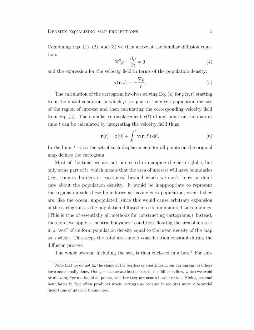
Density-equalizing map projections 5
Combining Eqs. (1), (2), and (3) we then arrive at the familiar diffusion equa-
tion:
∇2ρ −
∂ρ
∂t= 0 (4)
and the expression for the velocity field in terms of the population density:
v(r, t) = −∇ρ
ρ. (5)
The calculation of the cartogram involves solving Eq. (4) for ρ(r, t) starting
from the initial condition in which ρ is equal to the given population density
of the region of interest and then calculating the corresponding velocity field
from Eq. (5). The cumulative displacement r(t) of any point on the map at
time t can be calculated by integrating the velocity field thus:
r(t) = r(0) +
∫ t
0
v(r, t′) dt′. (6)
In the limit t → ∞ the set of such displacements for all points on the original
map defines the cartogram.
Most of the time, we are not interested in mapping the entire globe, but
only some part of it, which means that the area of interest will have boundaries
(e.g., country borders or coastlines) beyond which we don’t know or don’t
care about the population density. It would be inappropriate to represent
the regions outside these boundaries as having zero population, even if they
are, like the ocean, unpopulated, since this would cause arbitrary expansion
of the cartogram as the population diffused into its uninhabited surroundings.
(This is true of essentially all methods for constructing cartograms.) Instead,
therefore, we apply a “neutral buoyancy” condition, floating the area of interest
in a “sea” of uniform population density equal to the mean density of the map
as a whole. This keeps the total area under consideration constant during the
diffusion process.
The whole system, including the sea, is then enclosed in a box.1 For sim-
1Note that we do not fix the shape of the borders or coastlines in our cartogram, as others
have occasionally done. Doing so can create bottlenecks in the diffusion flow, which we avoid
by allowing free motion of all points, whether they are near a border or not. Fixing external
boundaries in fact often produces worse cartograms because it requires more substantial
distortions of internal boundaries.

6 Michael T. Gastner and M. E. J. Newman
plicity we consider only rectangular boxes, as most others have done also.2
Provided the dimensions Lx and Ly of the box are substantially larger than
the area to be mapped, the dimensions themselves do not matter. In the limit
Lx, Ly → ∞ the cartogram will be a unique deterministic mapping, indepen-
dent of the coordinate system used, with no overlapping regions. In practice,
we find that quite moderate system sizes are adequate—dimensions two to
three times the linear extent of the area to be mapped appear to give good
results. We also need to choose boundary conditions on the walls of the box.
This choice too has no great effect on the results, provided the size of the box
is reasonably generous. We use Neumann boundary conditions in which there
is no flow of population through the walls of the box.
The considerations above completely specify our method and are intuitive
and straightforward. The actual implementation of the method, if one wants a
calculation that runs quickly, involves a little more work. We solve the diffusion
equation in Fourier space, where it is diagonal, and back-transform before
integrating over the velocity field. With the Neumann boundary conditions,
the appropriate Fourier basis is the cosine basis, in which the solution to the
diffusion equation has the form
ρ(r, t) =4
LxLy
∑
k
ρ(k) cos(kxx) cos(kyy) exp(−k2t), (7)
where the sum is over all wave vectors k = (kx, ky) = 2π(m/Lx, n/Ly) with m,
n non-negative integers, and ρ(k) is the discrete cosine transform of ρ(r, t = 0):
ρ(k) =1
4(δkx,0 + 1)
(
δky ,0 + 1)
∫ Lx
0
∫ Ly
0
ρ(r, 0) cos(kxx) cos(kyy) dx dy, (8)
where δi,j is the Kronecker symbol. The velocity field v is then easily calculated
from Eqs. (5) and (7) and has components
vx(r, t) =
∑
kkxρ(k) sin(kxx) cos(kyy) exp(−k2t)
∑
kρ(k) cos(kxx) cos(kyy) exp(−k2t)
, (9a)
vy(r, t) =
∑
kkyρ(k) cos(kxx) sin(kyy) exp(−k2t)
∑
kρ(k) cos(kxx) cos(kyy) exp(−k2t)
. (9b)
2We discuss spherical cartograms briefly in Sec. 7.
Density-equalizing map projections 7
Equations (8) and (9) can be evaluated rapidly using the fast Fourier transform
and its back-transform respectively, both of which in this case run in time of
order LxLy log(LxLy). We then use the resulting velocity field to integrate
Eq. (6), which is a nonlinear Volterra equation of the second kind and can
be solved numerically by standard methods [5]. In practice it is the Fourier
transform that is the time-consuming step of the calculation and with the aid
of the fast Fourier transform this step can be performed fast enough that the
whole calculation runs to completion in a matter of seconds or at most minutes,
even for large and detailed maps.
3 Population density function
The description of our method tells, in a sense, only half the story of how
to create a cartogram. Before applying this or indeed any method, we need
to choose the starting density ρ(r) for the map. We can, by defining ρ(r)
in different ways, control the properties of the resulting cartogram, including
crucially the balance between accurate density equalization and readability.
Population density is not strictly a continuous function, since people are
themselves discrete and not continuous. To make a continuous function the
population must be binned or coarse-grained at some level. All methods of
constructing cartograms require one to do this, and no single accepted standard
approach exists. Part of the art of making a good cartogram lies in shrewd
decisions about the definition of the population density.
If we choose a very fine level of coarse-graining for the population density,
then the high populations in centers such as cities will require substantial local
distortions of the map in order to equalize the density. A coarser population
density will cause less distortion, resulting in a map with features that are
easier to recognize, but will give a less accurate equalization of the population
distribution. The most common choice made by others has been to coarse-
grain the population at the level of the (usually political) regions of interest.
For example, if one were interested in the United States, one might take the
population of each state and distribute it uniformly over the area occupied
by that state. This method can be used also with our cartogram algorithm
8 Michael T. Gastner and M. E. J. Newman
and we give some examples below. But we are not obliged to use it, and in
some cases it may be undesirable, since binning at the level of states erases
any details of population distribution below the state level.
On the other hand, if we use a finer resolution and allow for density vari-
ation within states then not only can the local distortions of the cartogram
become severe, but rapidly varying densities can also slow down the numerical
calculations. Regions with population density zero are particularly difficult
to deal with because the denominator in Eq. (5) becomes zero and hence the
velocity is undefined. In our work we circumvent these issues by first adding
a small constant to the density to get rid of zero values, and then applying a
spatially uniform Gaussian blur to the population density thus:
ρ(r) =1
2πσ2
∫ Lx
0
∫ Ly
0
ρraw(r′) exp
[
−(r′ − r)2
2σ2
]
dx′ dy′, (10)
where σ is the width of the Gaussian and ρraw is the unblurred density. Varying
the width σ of the blurring function is a convenient way to tune the cartogram
between accuracy and readability.
This blur can be performed rapidly in Fourier space, where the convolution
becomes a simple multiplication. Alternatively, we note that Eq. (10) is equal
to the density we would get if we simply allowed ρraw to diffuse for a time σ2
2,
so that we can also use Eq. (7) to calculate the Gaussian blur.
Ultimately the choice of population density function is up to the user of the
method, who must decide what particular features are most desirable in his
or her application. One advantage of our diffusion-based algorithm is that it
is entirely agnostic about this choice; the process of computing the cartogram
is decoupled from the calculation of the population density and, hence, is not
slanted in favor of one choice or another.
4 Applications I: Population cartograms and
aggregation
In the remainder of this paper we give several examples of the use of our
cartograms, focusing on the United States and using population data from

Density-equalizing map projections 9
(a) (b)
CityNew York
CityYork
New
Figure 2: Lung cancer cases among males in the state of New York, 1993-1997, as
in Fig. 1(a), but now plotted on population cartograms with (a) a coarse-grained
population density with σ = 50km and (b) a finer-grained population density with
σ = 1km.
the 2000 U.S. Census. First, we reexamine the New York lung cancer map,
Fig. 1(a), creating cartograms from population density functions with Gaussian
blurs of various widths, as described in the preceding section.3 In Fig. 2(a), we
show the data for cancer cases on a cartogram with only moderate blurring.
Although the map is visibly distorted, a reader familiar with the state of New
York would still be able to identify different regions because of the shape of
the state boundary. The distribution of cancer cases however is still visible
“clumped.”
In Fig. 1(b) we use a much finer Gaussian blur, creating a cartogram with
better population equalization and significantly greater distortion. Now the
virtue of this representation becomes strikingly clear. As the figure shows,
when we use a projection that truly equalizes the population density over the
map, there is no longer any obvious variation in the distribution of cases over
the state—the pattern appears random with more or less the same density of
cases everywhere. The shape of the map in Fig. 1(b) does not much resemble
the shape of the original any more, but this is the price we pay for equalizing
3A similar study using a different technique and for a smaller area was carried out by
Merrill [6].

10 Michael T. Gastner and M. E. J. Newman
the population almost perfectly.
We do not need to rely on eyesight for judging whether the distribution
of points in Fig. 1(b) is clustered. There are several statistical methods to
test spatial distributions for randomness. A particularly simple measure is
the Hopkins statistic H, a number between 0 and 1 whose expectation value
for random point patterns is 12. Higher values are a sign of clustering; lower
values indicate repulsion between points. Furthermore, it can be shown that
the value of the Hopkins statistic on random points is beta-distributed, which
allows us to calculate a p-value—the probability that the observed value of the
Hopkins statistic would occur if point position were purely random [7].
Calculating the Hopkins statistic for Fig. 1(a) gives a value of H = 0.89 ±
0.03 and a p-value < 10−16. This is of course hardly surprising since the distri-
bution shows very clear clustering around the major urban centers. But when
we perform the same calculation for the points on the cartogram Fig. 2(b) we
obtain H = 0.50 ± 0.03 consistent with a random distribution. Thus, the per
capita risk of lung cancer appears, by this calculation, to be the same every-
where. One might imagine that environmental effects such as pollution in big
cities could influence cancer rates, but we see no evidence of this. A more
careful analysis of course would have to take into account that people might
move between the time when they are exposed to a carcinogen and the time
when they develop cancer. However, Figure 1(a), despite its impressive clus-
tering, definitely cannot be taken as evidence that there are high-risk regions
of New York state for cancer. This finding is consistent with medical evidence
that lung cancer is caused by individual behavior rather than environmental
causes, with smoking alone responsible for 90% of all cases worldwide [8].
Not all threats to our well-being, however, are uniformly distributed. In
Fig. 3(a) we plot each of the 2301 homicides that occurred in the state of
California in the year 2001 on an equal-area map, and the map again shows
clear clustering around urban areas, particularly the Greater Los Angeles area.
Switching once again to a high-resolution population cartogram, Fig. 3(b), we
see that the points become more spread out, as before, but this time it is clear
that the distribution is far from random. Especially in the southwestern part of
Los Angeles the density is clearly higher than average even on the cartogram.

Density-equalizing map projections 11
Sacramento
SanFrancisco
Oakland
San Jose
Fresno
Los Angeles
Riverside
Anaheim
Long BeachSanta Ana
San Diego
Sacramento
SanFrancisco
Oakland
San Jose
Fresno
Los Angeles
Riverside
Anaheim
Long BeachSanta Ana
San Diego
(a) (b)
Figure 3: Homicides in California in 2001. (a) Equal-area projection. (b) Population
cartogram. Data from the California Department of Health Services.
The Hopkins statistic confirms this impression. Its value of 0.68± 0.04 for the
cartogram indicates that there is clustering even on the cartogram and the p-
value for complete spatial randomness is below 10−8, meaning the probability
that we would get a point pattern such as this purely by chance is below
one in a hundred million. Undoubtedly, some parts of the state experience a
statistically significant higher number of homicides per capita than others.
For the last example in this section we look at technological rather than
social data and analyze the geographic distribution of the Internet in the con-
tiguous United States. The Internet is a network of computers and routers
connected by optical fiber. Computers belonging to the same company or or-
ganization are typically grouped together into subnetworks called Autonomous
Systems (ASes) or routing domains that share a single external routing policy.
Here we treat each AS as a single point in geographic space; we have created
a map of the Internet using the software tool NetGeo,4 which can return ap-
proximate latitude and longitude for a specified AS. The positions of the 7049
4http://www.caida.org/tools/utilities/netgeo

12 Michael T. Gastner and M. E. J. Newman
Seattle
Boston
Minneapolis
New York
Detroit
Chicago
WashingtonD. C.
SanFrancisco
Denver
San Jose
LosAngeles
Memphis
AtlantaSan Diego
Phoenix
Dallas
Jacksonville
Houston Miami
Seattle
Boston
Minneapolis
New York
DetroitChicago
Washington,D. C.
SanFrancisco
Denver
San Jose
LosAngeles
Memphis
AtlantaSan Diego
Phoenix
Dallas Jacksonville
HoustonMiami
(a)
(b)
Figure 4: Autonomous systems on the Internet in the contiguous United States
(March 2003). (a) Equal-area projection. (b) Population cartogram.
ASes in the lower 48 states in March 2003 is shown in Fig. 4(a).
That ASes on this equal-area map appear heavily clustered in cities comes
as no surprise since there are more people in the cities. Switching to a car-

Density-equalizing map projections 13
togram, Fig. 4(b), we find in this case that, like the homicides, the ASes
become more uniform, but are still concentrated around the cities. Some ur-
ban areas appear particularly dense, such as Silicon Valley (west of San Jose),
Manhattan (New York City), or Washington, DC. Other cities, by contrast,
appear to have no more ASes per capita than average—for example, Detroit,
Memphis, and Jacksonville. The Hopkins statistic for the distribution on the
cartogram takes a value of H = 0.80 ± 0.04, and the random distribution is
firmly ruled out (the p-value is < 10−16). In the early days of the Internet it was
often claimed that geographic position would become unimportant thanks to
high-speed data transmission and easy access to information from everywhere.
Apparently, this has not happened.
5 Applications II: Cartograms based on other
density functions
The cartograms shown so far have all been based on human population density,
which is certainly the most common type of cartogram. Other types, however,
are also possible and we give some examples in this section.
For our first example we examine the usage and production of energy in
the United States. Each year, the US Energy Information Administration
estimates each state’s total energy consumption, including electricity, coal,
gas, petroleum, wood, and alternative energy sources [9]. For instance, in
the year 2000 the United States consumed a total of 98 quadrillion British
thermal units of energy. The use of energy varies greatly between the states,
with Texas, for example, consuming 70 times as much energy as Vermont.
In Fig. 5(a) we show a cartogram in which states are scaled according to
their total energy consumption during the year 2000. The cartogram appears
quite similar to the population cartogram in Fig. 4(b), indicating that energy
consumption per capita is roughly the same in most parts of the country. On
closer inspection one might detect that the biggest state in Fig. 4(b), California,
has been overtaken in Fig. 5(a) by what was formerly the second biggest state,
Texas. New York and Florida have also become smaller, Pennsylvania and

14 Michael T. Gastner and M. E. J. Newman
AL
AK
AZ
AR
CACO
CT
DE
DC
FL
GA
HI
ID
IL IN
IAKS
KY
LA
ME
MD
MAMIMN
MS
MO
MT
NENV
NH
NJNM
NY
NC
ND
OH
OK
OR
PARI
SC
SD
TNTX
UT
VT
VA
WA
WV
WIWY
AK
KY
LA
NM
OK
PA
TX
WV
WY
(a)
(b)
Figure 5: (a) A cartogram of the United States in which the sizes of states are
proportional to their total energy consumption. (b) A similar cartogram for energy
production. States are the same color in (a) and (b).
Louisiana larger, but all in all the changes are relatively minor—population
density explains energy consumption quite well.
But now look at Fig. 5(b), which shows total energy production by state,
again from figures compiled by the Energy Information Administration for
Density-equalizing map projections 15
the year 2000 and including crude oil, gas, and coal as well as electricity
not generated from fossil fuels [10]. This cartogram gives a very different
perspective on the country. A small number of states, most notably Texas,
Louisiana, and Wyoming, dominate the country’s energy production, the first
two because of their wealth in oil and gas, the third because of its abundance of
coal. Total US energy production is 61 quadrillion British thermal units, which
is only 62% of consumption—the difference is made up of imported energy—so
the total area of Fig. 5(b) is smaller than that of Fig. 5(a) by the same factor.
Figures 5(a) and (b) together highlight the substantial redistribution of energy
from producer to consumer in the United States.
For our second example of a cartogram not based on population density
we examine the media attention paid to different parts of the country. Anyone
who reads or watches the news in the United States (and similar observations
probably apply in other countries as well) will have noticed that the geograph-
ical distribution of news stories is not uniform. Even allowing for population,
a few cities, notably New York and Washington, DC, get a surprisingly large
fraction of the attention while other places get little. Apparently some loca-
tions loom larger in our mental map of the nation than others, at least as
presented by the major media. We can turn this qualitative idea into a real
map using our cartogram method.
We have taken about 72 000 newswire stories from November 1994 to April
1998,5 and extracted from each the “dateline,” a line at the head of the story
that gives the date and the location that is the main focus of the story. Binning
these locations by state, we then produce a map in which the sizes of the US
states are proportional to the number of stories concerning that state over the
time interval in question. The result is shown in Fig. 6.
The stories are highly unevenly distributed. New York City alone con-
tributes 20 000 stories to the corpus, largely because of the preponderance
of stories about the financial markets, and Washington, DC another 10 000,
5Data from the Associated Press Worldstream wire service, compiled and distributed
on CD-ROM by the Linguistic Data Consortium (North American News Text Supplement
1998).

16 Michael T. Gastner and M. E. J. Newman
AK
HI
CA
WA
AZ
CO
TX
MNMI
IL
PA
GA
DC
FL
NY
MA
NJ
Figure 6: Cartogram in which the sizes of states are proportional to the frequency
of their appearance in news stories. States are the same color as in Fig. 5.
largely political stories. We chose to bin by state to avoid large distortions
around the cities that are the focus of most news stories. We made one excep-
tion however: since New York City had far more hits than any other location
including the rest of the state of New York (which had around 1000), we split
New York State into two regions, one for the greater New York City area and
another for the rest of the state.
The cartogram offers a dramatic depiction of the distribution of US news
stories. The map is highly distorted because the patterns of reporting show
such extreme variation. Washington, DC, for instance, which normally would
be virtually invisible on a map of this scale, becomes the second largest “state”
in the union. (The District of Columbia is not, technically, a state.) People
frequently overestimate the size of the northeastern part of the United States
by comparison with the middle and western states, and this map may give us
a clue as to why. Perhaps people’s mental image of the United States is not
really an inaccurate one; it is simply based on things other than geographical
area, such as the attention regions receive in the media.
Numerous other possible applications of cartograms come readily to mind,
such as visualizations of gross regional products, numbers of people belong-

Density-equalizing map projections 17
ing to certain ethnic groups, sales of consumer goods, and so forth. Diffusion
cartograms might also have applications outside geography. One possibility is
the creation of a homunculus, a representation of the human body in which
each bodily part is scaled in proportion to the size of the brain region devoted
to it [11]. Such representations are usually constructed as two-dimensional
plots, but there is no reason in theory why one could not create a fully three-
dimensional homunculus; the diffusion process is easily generalized to any num-
ber of dimensions.
6 Performance of the algorithm
An important consideration with any method for producing cartograms is ef-
ficiency. In many cases one would like to create cartograms interactively for
data exploration, which means that program run times for producing them
should be limited to seconds, or at most a few minutes for the most complex
cartograms such as the larger country-sized ones shown above. In this sec-
tion we provide some figures on run times and analysis of the efficiency of our
cartogram method.
We have implemented our algorithm as a C program and it is this imple-
mentation that we analyze here. (No doubt faster implementations than ours
are possible, given time and effort, but we believe ours to give a good gen-
eral indication of the speeds attainable.) We analyze the performance of the
program in calculating a cartogram of the lower 48 states and the District of
Columbia with each region scaled according to population.
The program goes through the following steps in creating the cartogram.
First, the polygons making up the regions of the input map are read from
ASCII files, along with data on the population of each region. Then, a fine
square grid is created and filled with the initial density distribution. The grid
spacing has to be chosen such that the smallest polygon is covered by at least
a few grid points. For the present example we chose a 1024×512 grid, which is
adequate to resolve the smallest region, the District of Columbia. The program
then evaluates the cartogram transformation for each grid point by solving the
diffusion equation as outlined in Sec. 2. The positions of the vertices of each

18 Michael T. Gastner and M. E. J. Newman
polygon are calculated by piecewise bilinear transformations from the points of
the distorted grid.6 For this example our program runs to completion within
312
minutes on a standard desktop computer with a 2.8GHz Intel Pentium IV
processor. Total memory used is 22MB.
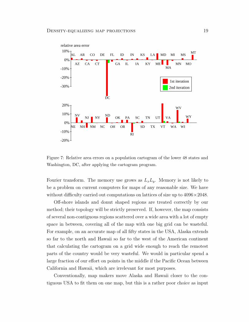
Another important measure is the accuracy of the algorithm. How precisely
are the final areas proportional to population? We measure the fractional error
in each region’s area by calculating the quantity
relative error =area of state on cartogram × total population of all states
total area of all states on map × population of state−1.
(11)
The results are shown as the red bars in Fig. 7. Most states are within ±10%
of their target value, with the exception of Washington, DC, and Rhode Is-
land, which are too small, and Vermont and West Virginia, which are too big.
The inaccuracies are caused partly by sampling the density on a finite grid
and partly by approximations made by the integrator routine. For most appli-
cations these errors are probably acceptable. On the input map the densities
vary by more than a factor of 1600 between the densest region, Washington,
DC, and the sparsest, Wyoming. On the cartogram the extreme densities—
now Washington, DC, and West Virginia—only differ by a factor of about 2,
or almost three orders of magnitude less.
However, if the errors are a major concern there is a simple way to improve
the result, namely running the algorithm again starting from the cartogram
produced by the first run. The time taken is the same as before, but the
area errors are now reduced to less than 3.5% in all cases (the green bars in
Fig. 7) which is certainly much less than can be detected by eye. If even
higher accuracy is needed one can of course run the algorithm as many times
as needed. Alternatively, one could make the initial square grid finer from
the start at the expense of longer run-times. For an Lx × Ly grid the time
needed for a single run scales as LxLy log(LxLy), the bottleneck being the fast
6It would be entirely possible—and in some cases quicker—to transform the polygon
vertices separately using the diffusion equation, but the grid-based method described here is
simpler and more general and gives results essentially as good; the grid is fine enough that
the errors introduced by the interpolation are small.
Density-equalizing map projections 19
-30%
-20%
-20%
-10%
-10%
0%
0%
10%
10%
20%
relative area error
AL
AZ
AR
CA
CO
CT
DE
DC
FL
GA
ID
IL
IN
IA
KS
KY
LA
ME
MD
MA
MI
MN
MS
MO
MT
NE
NV
NH
NJ
NM
NY
NC
ND
OH
OK
OR
PA
RI
SC
SD
TN
TX
UT
VT
VA
WA
WV
WI
WY
1st iteration
2nd iteration
Figure 7: Relative area errors on a population cartogram of the lower 48 states and
Washington, DC, after applying the cartogram program.
Fourier transform. The memory use grows as LxLy. Memory is not likely to
be a problem on current computers for maps of any reasonable size. We have
without difficulty carried out computations on lattices of size up to 4096×2048.
Off-shore islands and donut shaped regions are treated correctly by our
method; their topology will be strictly preserved. If, however, the map consists
of several non-contiguous regions scattered over a wide area with a lot of empty
space in between, covering all of the map with one big grid can be wasteful.
For example, on an accurate map of all fifty states in the USA, Alaska extends
so far to the north and Hawaii so far to the west of the American continent
that calculating the cartogram on a grid wide enough to reach the remotest
parts of the country would be very wasteful. We would in particular spend a
large fraction of our effort on points in the middle if the Pacific Ocean between
California and Hawaii, which are irrelevant for most purposes.
Conventionally, map makers move Alaska and Hawaii closer to the con-
tiguous USA to fit them on one map, but this is a rather poor choice as input

20 Michael T. Gastner and M. E. J. Newman
to our cartogram program because moving them closer to the lower 48 states
can cause their diffusion patterns to interact with those of the lower 48, in-
fluencing the final shape of the cartogram.7 (The areas of the states would
still be correct, but their shapes would be distorted.) A better solution is
to construct separate cartograms for Alaska and Hawaii, and then afterward
place them next to the cartogram for the continental USA in the traditional
fashion. Some care must be taken to make sure the population scale of the
different cartograms matches correctly. The cartograms in Figs. 5 and 6 were
constructed in this manner.
7 Discussion and conclusions
In this paper we have described a new general method for constructing density-
equalizing projections or cartograms, which provide an invaluable tool for the
presentation and analysis of geographic data. Our method is simpler than
many earlier methods, allowing for rapid calculations, while generating accu-
rate and readable maps. The method allows its users to choose their own
balance between good density equalization and low distortion of map regions,
making it flexible enough for a wide variety of applications. We have presented
a number of examples of the use of our cartograms to represent human data.
We have implemented our method as a C program which is available from
our web site.8 Directly embedding the algorithm as a function in GIS software
packages should also be straightforward. For even the most complex examples,
the program achieves good density-equalization on the time scale of a few
minutes with current computing resources.
One interesting direction for future research is the creation of cartograms in
spaces that are not flat. Here we have assumed that our mapped space is flat,
7Islands just off the coast, like Long Island, will of course influence diffusion on the
mainland too, but this is correct because these islands really are in the “neighborhood”
and their influence should be felt. The high population of Brooklyn and Queens on Long
Island for example should expand and repel the mainland as in Fig. 2, thereby preserving
the topology of map.8http://www-personal.umich.edu/~mgastner

Density-equalizing map projections 21
but this is never strictly true since the surface of the Earth is curved. Even
for an area as large as the contiguous United States it is usually legitimate to
neglect curvature when a suitable projection is used for the input map (such
as the Albers conic projection used here). For a larger area—a cartogram of
the entire world, for instance—this would no longer be possible. In that case
we would have to solve the diffusion equation (4) on the surface of the sphere
in spherical coordinates:
1
sin θ
∂
∂θ
(
sin θ∂ρ
∂θ
)
+1
sin2 θ
∂2ρ
∂φ2=
∂ρ
∂t. (12)
The solution can be expressed in terms of spherical harmonics Ylm(θ, φ) thus:
ρ(θ, φ, t) =∞
∑
l=0
l∑
m=−l
ρlmYlm(θ, φ) exp[−l(l + 1)t] (13)
where
ρlm =
∫
Y ∗
lm(θ, φ)ρ(θ, φ, t = 0) dΩ. (14)
As in the Cartesian case we can now use Eq. (5) to solve for the velocities
vθ(θ, φ, t) = −1
ρ
∂ρ
∂θ
=
∑
∞
l=0
∑l
m=−l+1
√
l(l + 1) − m(m − 1)ρlmYl,m−1(θ, φ)eiφe−l(l+1)t
2∑
∞
l=0
∑l
m=−l ρlmYlm(θ, φ) exp[−l(l + 1)t]
−
∑
∞
l=0
∑l−1m=l
√
l(l + 1) − m(m + 1)ρlmYl,m+1(θ, φ)e−iφe−l(l+1)t
2∑
∞
l=0
∑l
m=−l ρlmYlm(θ, φ)e−l(l+1)t,
vφ(θ, φ, t) = −1
ρ sin θ
∂ρ
∂φ
= −i
∑
∞
l=0
∑l
m=−l mρlmYlm(θ, φ)
sin θ∑
∞
l=0
∑l
m=−l ρlmYlm(θ, φ)e−l(l+1)t. (15)
To solve Eqs. (13), (14), and (15) efficiently we need the equivalent of the fast
Fourier forward and backward transforms for spherical harmonics. Although
such transforms exist, implementations are far from trivial and a current field
of research [12].

22 Michael T. Gastner and M. E. J. Newman
Acknowledgments
The authors would like to thank the staff of the University of Michigan’s
Numeric and Spatial Data Services for their help with the geographic data,
and Dragomir Radev for useful discussions about the geographic distribution
of news messages. This work was funded in part by the National Science
Foundation under grants DMS–0234188 and DMS–0405348 and by the James
S. McDonnell Foundation.
References
[1] S. M. Guseyn-Zade and V. S. Tikunov, “Analog methods in the compila-
tion of areal transformed images,” Mapping Sciences and Remote Sensing,
vol. 31, pp. 49–65, 1994.
[2] D. Dorling, “Area cartograms: Their use and creation,” Concepts and
Techniques in Modern Geography (CATMOG), vol. 59, 1996.
[3] B. D. Dent, Cartography: Thematic Map Design. Boston:
WCB/McGraw-Hill, 5th ed., 1999.
[4] W. Tobler, “Thirty five years of computer cartograms,” Annals of the
Association of American Geographers, vol. 94, pp. 58–73, 2004.
[5] W. H. Press, S. A. Teukolsky, W. T. Vetterling, and B. P. Flannery,
Numerical Recipes in C. Cambridge: Cambridge University Press, 1992.
[6] D. W. Merrill, “Use of a density equalizing map projection in analysing
childhood cancer in four California counties,” Statistics in Medicine,
vol. 20, pp. 1499–1513, 2001.
[7] B. Hopkins, “A new method for determining the type of distribution of
plant individuals,” Annals of Botany, vol. 18, pp. 213–227, 1954. Ap-
pendix by J. G. Skellam.
[8] A. Spira, J. Beane, V. Shah, G. Liu, F. Schembri, X. Yang, J. Palma, and
J. S. Brody, “Effects of cigarette smoke on the human airway epithelial

Density-equalizing map projections 23
cell transcriptome,” Proceedings of the National Academy of Sciences of
the United States of America, vol. 101, pp. 10143–10148, 2004.
[9] “State Energy Data Report 2000,” technical report, Energy Information
Administration, Office of Energy Markets and End Use, U.S. Department
of Energy, Washington, DC.
[10] http://www.eia.doe.gov/emeu/states/2000StateEnergy Sep2003.xls.
[11] J. Mitchell, ed., The Random House Encyclopedia, p. 667. New York:
Random House, 3rd ed., 1990.
[12] D. M. Healy, D. N. Rockmore, P. J. Kostelec, and S. Moore, “FFTs for
the 2-sphere—improvements and variations,” Journal of Fourier Analysis
and Applications, vol. 9, pp. 341–385, 2003.