
Demystifying the Chinese Housing Boom - NBER
73
Demystifying the Chinese Housing Boom * Hanming Fang, Quanlin Gu, Wei Xiong, and Li‐An Zhou April 2015 Abstract We construct housing price indices for 120 major cities in China in 2003‐2013 based on sequential sales of new homes within the same housing developments. By using these indices and detailed information on mortgage borrowers across these cities, we find enormous housing price appreciation during the decade, which was accompanied by equally impressive growth in household income, except in a few first‐tier cities. While bottom‐income mortgage borrowers endured severe financial burdens by using price‐to‐income ratios over eight to buy homes, their participation in the housing market remained steady and their mortgage loans were protected by down payments commonly in excess of 35 percent. As such, the housing market is unlikely to trigger an imminent financial crisis in China, even though it may crash with a sudden stop in the Chinese economy and act as an amplifier of the initial shock. * Fang is with the Department of Economics, University of Pennsylvania and the NBER, email: [email protected]. Gu and Zhou are with the Department of Applied Economics, Guanghua School of Management, Peking University, emails: [email protected] (Gu) and [email protected] (Zhou). Xiong is with the Department of Economics and Bendheim Center for Finance, Princeton University and the NBER, email: [email protected]. This paper is prepared for NBER Macro Annual (Volume 30). We are grateful to the editors, Marty Eichenbaum and Jonathan Parker, our discussants, Erik Hurst and Martin Schneider, as well as seminar participants at Bank of America Merrill Lynch, Harvard University and Princeton University for helpful discussions and constructive comments. We also thank Sean Dong, Qing Gong, Min Wu, and Yu Zhang for excellent research assistance.
Transcript of Demystifying the Chinese Housing Boom - NBER

Demystifying the Chinese Housing Boom*
Hanming Fang, Quanlin Gu, Wei Xiong, and Li‐An Zhou
April 2015
Abstract
We construct housing price indices for 120 major cities in China in 2003‐2013 based on sequential sales of new homes within the same housing developments. By using these indices and detailed information on mortgage borrowers across these cities, we find enormous housing price appreciation during the decade, which was accompanied by equally impressive growth in household income, except in a few first‐tier cities. While bottom‐income mortgage borrowers endured severe financial burdens by using price‐to‐income ratios over eight to buy homes, their participation in the housing market remained steady and their mortgage loans were protected by down payments commonly in excess of 35 percent. As such, the housing market is unlikely to trigger an imminent financial crisis in China, even though it may crash with a sudden stop in the Chinese economy and act as an amplifier of the initial shock.
* Fang is with the Department of Economics, University of Pennsylvania and the NBER, email: [email protected]. Gu and Zhou are with the Department of Applied Economics, Guanghua School of Management, Peking University, emails: [email protected] (Gu) and [email protected] (Zhou). Xiong is with the Department of Economics and Bendheim Center for Finance, Princeton University and the NBER, email: [email protected]. This paper is prepared for NBER Macro Annual (Volume 30). We are grateful to the editors, Marty Eichenbaum and Jonathan Parker, our discussants, Erik Hurst and Martin Schneider, as well as seminar participants at Bank of America Merrill Lynch, Harvard University and Princeton University for helpful discussions and constructive comments. We also thank Sean Dong, Qing Gong, Min Wu, and Yu Zhang for excellent research assistance.

1
There have been growing concerns across the global economic and policy communities
regarding the decade‐long housing market boom in China, which has the second largest
economy in the world and has been the major engine for global economic growth during the
past decade. News in recent months seems to suggest that the housing boom might be slowing
down. A main concern is that a housing market meltdown might severely damage the Chinese
economy, which in turn might generate contagious effects across the world and slow down the
fragile global economy that has just emerged from a series of crises that originated in the U.S.
and Europe. In particular, critics are concerned that soaring housing prices and the enormous
construction boom throughout the country might cause China to follow in the footsteps of
Japan, which had an economic lost decade after its housing bubble burst in the early 1990s.
How much have housing prices in China appreciated during the last decade? How did the
price appreciation vary across different Chinese cities? Did the soaring prices exclude low‐
income households from participating in the housing markets? How much financial burden did
households face in buying homes? Addressing these questions is crucial for systematically
assessing the risk to the Chinese economy presented by its housing market. We address these
questions by taking advantage of a comprehensive data set of mortgage loans issued by a major
Chinese commercial bank from 2003‐2013. Specifically, we construct a set of housing price
indices for 120 major cities in China, which allows us to evaluate housing price fluctuations
across these cities, in conjunction with the growth of households’ purchasing power and stock
price fluctuations. The detailed mortgage data also allow us to analyze the participation of low‐
income households in housing markets and the financial burdens faced by low‐income home
buyers.
Due to the nascent nature of the Chinese housing market, there are relatively few repeat
home sales available for building Case‐Shiller type repeated sales housing indices. Instead, we
take advantage of the large number of new housing developments in each city and build a
housing price index for the city based on sales over time of new homes within the same
developments, which share similar characteristics and amenities. Consistent with casual
observations made by many commentators, our price indices confirm enormous housing price

2
appreciation across China in 2003‐2013. In first‐tier cities, which include the four most
populated and most economically important metropolitan areas in China‐‐ Beijing, Shanghai,
Guangzhou, and Shenzhen‐‐ housing prices had an average annual real growth rate of 13.1
percent during this decade. Our sample also covers 31 second‐tier cities, which are
autonomous municipalities, provincial capitals, or vital industrial/commercial centers, and 85
other third‐tier cities, which are important cities in their respective regions. Housing prices in
second‐tier cities had an average annual real growth rate of 10.5 percent; third‐tier cities had
an average annual real growth rate of 7.9 percent. These growth rates easily surpass the
housing price appreciation during the U.S. housing bubble in the 2000s and are comparable to
that during the Japanese housing bubble in the 1980s.
Despite the enormous price appreciation, the Chinese housing boom is different in nature
from the housing bubbles in the U.S. and Japan. Our analysis offers several important
observations that are useful for understanding the Chinese housing boom. First, as banks in
China imposed down payments of over 30 percent on all mortgage loans, banks are protected
from mortgage borrowers’ default risk even in the event of a sizable housing market meltdown
of 30 percent. This makes a U.S. style subprime credit crisis less likely in China.
Second, while the rapid housing price appreciation has been often highlighted as a concern
for the Chinese housing market, the price appreciation was accompanied by equally spectacular
growth in households’ disposable income‐‐‐an average annual real growth rate of about 9.0
percent throughout the country during the decade, with the exception of a lower average
growth rate of 6.6 percent in the first‐tier cities. This joint presence of enormous housing price
appreciation and income growth contrasts the experiences during the U.S. and Japanese
housing bubble. Even during the Japanese housing bubble in late 1980s, the Japanese economy
was growing at a more modest rate than that of China. The enormous income growth rate
across Chinese cities thus provides some assurance to the housing boom and, together with the
aforementioned high mortgage down payment ratios, renders the housing market an unlikely
trigger for an imminent financial crisis in China.

3
Third, despite the enormous housing price appreciation over the decade, the participation
of low‐income households in the housing market remained stable. Specifically, we analyze the
financial status of mortgage borrowers with incomes in the bottom 10 percent of all mortgage
borrowers in each city for each year. By mapping the incomes of these marginal home buyers
into the income distribution of the urban population in the city, we find that they came from
the low‐income fraction of the population, roughly around the 25th percentile of the
distribution in the first‐tier cities and around the 30th percentile in the second‐tier cities.
Fourth, while these low‐income home buyers were not excluded from the housing market,
they did endure enormous financial burdens in buying homes at price‐to‐income ratios of
around eight in second‐ and third‐tier cities and, in some years, even over ten in first‐tier cities.
In concrete terms, this means that a household paid eight times its annual disposable income to
buy a home. In order to obtain a mortgage loan, it had to make a down payment of at least 30
percent, and more typically 40 percent, of the home price, which was equivalent to 2.4 times
to 3.2 times the household’s annual income. Suppose that the household made a down
payment of 40 percent and took a mortgage loan for the other 60 percent of the home price,
which would be 4.8 times its annual income. A modest mortgage rate of 6 percent, which is low
relative to the actual rate observed during the decade, would require the household to use
nearly 30 percent of its annual income to pay for the interest on the mortgage loan.
Furthermore, paying the mortgage would consume another 16 percent of its annual income
used a linear amortization even if the mortgage had a maximum maturity of 30 years. Together,
buying the home entailed saving 3.2 times the annual household income to make the down
payment and another 45 percent of its annual income to service the mortgage loan.
To explain the willingness of households to endure such severe financial burdens for a home,
it is important to take into account the households’ expectations. To the extent that urban
household income in China has been rising steadily during the studied period, as well as in the
previous two decades, many households may expect their income to continue growing at this
rate. At a 10 percent nominal income growth rate, a household’s income in five years would
grow to 1.6 times of its initial income and the ratio of current housing price to its future income

4
in five years would drop to five. Thus, a high expected income growth rate renders the
aforementioned financial burdens temporary.
Such high income growth expectations might have resulted from extrapolative behavior as
emphasized by Barberis, Shleifer, and Vishny (1998) and Shiller (2000), or from contagious
social dynamics between households as modeled by Burnside, Eichenbaum, and Rebelo (2013).
Recently, Pritchett and Summers (2014) examine historical data on growth rates and
demonstrate that regression to the mean is the single most robust and empirically relevant fact
about cross‐country growth rates. Thus, they argue that while China might continue to grow for
another two decades at a 9, or even a 7 or 6 percent rate, such continued rapid growth rate
would be an extraordinary event, given the powerful force of regression to the mean, which
had averaged 2 percent in the cross‐country data with a standard deviation of 2 percent. If so,
the high expectation of future income growth, which might have been a key driver of the
observed enormous price‐to‐income ratios, may not be sustainable and thus presents an
important source of risk to the housing market. When China’s growth rate eventually regresses
to the mean, and especially when China experiences a sudden stop, households’ expectations
may crash. In such a case, the large price‐to‐income ratios have substantial room to contract,
which in turn could act as an amplifier of the initial shock that triggers the economic slowdown.
Frictions in the Chinese financial system might also have contributed to the high housing
prices across Chinese cities, as reflected by the large price‐to‐income ratios endured by
households. It is well‐known that the spectacular economic growth in China since the 1980s has
been accompanied by a high savings rate, e.g., Yang, Zhang, and Zhou (2013). Due to stringent
capital controls, savers cannot invest their savings in international capital markets and, instead,
have only a few domestic investment vehicles. Bank deposit accounts have remained the
predominant investment vehicle, with assets totaling near 100 trillion RMB in 2013, despite the
fact that the real one‐year deposit rate averaged only 0.01 percent in 2003‐2013. While the
Chinese stock market experienced dramatic growth during this decade, it was still relatively
small, with a capitalization of slightly less than 20 trillion RMB in 2013. The size of bond markets
was even smaller. Facing this largely constrained investment set, it has been common for

5
households to treat housing as an alternative investment vehicle, which also helps explain their
willingness to pay dearly for housing.
From an investment perspective, it is interesting to note a tale of two markets at the time of
the world economic crisis in 2008‐2009. During this period, the Chinese economy faced
tremendous pressure. Nevertheless, the housing market in China remained strong. Housing
prices in first‐tier cities suffered a modest drop of about 10 percent, and recovered more than
the loss shortly after the crisis. Housing prices in second‐ and third‐tier cities continued to rise
throughout the period after 2008. This experience was in sharp contrast to the dramatic decline
of over 60 percent in the Chinese stock market in 2008‐‐which has not been recovered even to
date. To understand this puzzling contrast, we argue that the frequent policy interventions by
the central government and the heavy reliance of local governments on land sales revenue for
their fiscal budget might have emboldened many households to believe that the housing
market is too important to fall and that the central government would institute policies to
support the housing market if necessary.
There are divergent views about the Chinese housing boom. Chow and Niu (2014) use a
simultaneous equations framework to analyze the demand and supply of residential housing in
urban China in 1987‐2012 and find that the rapid housing price growth can be well explained by
the force of demand and supply, with income determining demand and construction costs
affecting supply. Deng, Gyourko, and Wu (2014b) are far more concerned by the risk in the
Chinese housing market. In particular, they present evidence of a rapid increase in housing
supply and housing inventory held by developers in various major cities in recent years.
Different from these studies, we provide an informed account of the demand side by
thoroughly analyzing characteristics of mortgage borrowers. Our analysis leads us to take a
more balanced stand between these two contrasting views. On the comforting side, the rapid
income growth, which accompanied the enormous housing price appreciation, helped support
the steady participation by low‐income households in the housing market. On the concerning
side, high expectations about future income growth might have motivated low‐income

6
households to buy homes by undertaking substantial financial burdens, causing them to be
particularly vulnerable to future sudden stops in the Chinese economy.
This paper is organized as follows. Section 1 briefly describes some institutional background.
We introduce the housing price indices in Section 2 and then discuss the housing price boom
across three tiers of cities in Section 3. Section 4 summarizes characteristics of mortgage
borrowers, and Section 5 discusses housing as an investment vehicle. Section 6 provides some
conceptual discussion. We summarize the role of government in Section 7 and discuss several
sources of risk in Section 8.
1. Institutional Background
The development of housing markets in mainland China is a relatively new phenomenon.
From the 1949 founding of the People’s Republic of China to 1978, all land was publicly owned
and the Chinese constitution prohibited any organization or individual from buying, selling,
leasing, or transferring land. Housing was allocated through a working unit‐employee linkage as
a form of in‐kind compensation, with the size and location of homes depending on the length of
employment and the size of the household, among other factors. In 1978, per capita residential
area in urban areas was 3.6 square meters, which was even lower than that in 1949.
To reform (and to a large extent privatize) the state‐owned enterprises in the mid‐1980s, it
was considered necessary to introduce an alternative housing system that would delink home
allocation from employment. An important milestone occurred in 1988 when the Chinese
constitution was amended to allow for land transactions, which set the legal stage for the
privatization of housing in China.1
Comprehensive housing reform was initiated in 1994 when employees in the state sector
were allowed to purchase full or partial property rights to their current apartment units at
subsidized prices. Nascent markets for homes, known as “commodity houses,” emerged in
1 Under current law, land used to build residential properties is leased for a term of 70 years; after the expiration of the lease period, the right to use the land and the property will no longer belong to the current owner. It is commonly presumed that the law will eventually be amended so that property owners will be allowed to renew the leases.

7
some large cities in early 1990s; but they grew rapidly only after 1998 when the central
government completely abolished the traditional model of housing allocation as an in‐kind
benefit and privatized housing properties of all urban residents.
Also in 1998, partly as a response to the adverse effects of the 1997 Asian Financial Crisis,
the Chinese government established the real estate sector as a new engine of economic growth.
As an important impetus to the development of private housing markets, China’s central bank,
the People’s Bank of China (PBC), outlined the procedures for home buyers to obtain residential
mortgages at subsidized interest rates in 1998.2 Moreover, between 1998 and 2002, the PBC
lowered the mortgage interest rate five times to encourage home purchases. By 2005, China
had become the largest residential mortgage market in Asia. According to a PBC report
published in 2013, financial institutions made a total of 8.1 trillion RMB in mortgage loans in
2012, accounting for 16 percent of all bank loans in that year. At the same time, the PBC also
developed policies to encourage housing development, including broadening the scope of
development loans and allowing pre‐sales by developers.
[Figure 1 about Here]
These policies were effective in stimulating both the demand and supply of residential
housing. During this period, home sales maintained about 15 percent of annual growth on
average, and areas of residential housing under construction grew even faster, reaching about
18 percent of annual growth. Figure 1 provides a rough estimate of the supply of newly
completed residential housing from 2002‐2013 by city tier, measured by completed areas in
each city and each year divided by the city’s urban population in 2012.
It is common in China to separate cities into three tiers. The first tier includes the four cities
with the largest population and economic importance in China‐‐ Beijing, Shanghai, Guangzhou,
and Shenzhen. Our data cover all of these first tier cities. The second tier is comprised of
Tianjing and Chongqing (the two autonomous municipalities other than Beijing and Shanghai)
2 See Appendix A for detailed information about mortgage loans in China.

8
and capital cities of the 24 provinces3 and 9 other cities, which are typically vital industrial or
commercial centers. Our data cover 31 of these 35 second‐tier cities. There is not a commonly
used list for third‐tier cities. Instead, we group 85 other cities in our sample as the third tier.
Appendix B provides a list of all cities in our sample.
The construction boom of residential housing in first‐tier cities started in the late 1990s,
followed by that of second‐ and third‐tier cities in the early 2000s. In Figure 1, new construction
of residential housing showed a similar growth rate across the three tiers of cities in 2002‐2005.
From 2005, the new construction in first‐tier cities had slowed down substantially due to the
shortage of land supply in these cities, while the supply in second‐ and third‐tier cities
continued to grow at similar rate as before. The growth rate in third‐tier cities was especially
strong. Some estimates suggest that investment to residential housing accounted for 25
percent of total fixed asset investment and contributed to roughly one‐sixth of China’s GDP
growth (Barth et al., 2012).
[Figure 2 about Here]
The development of the housing market was also accompanied by an urbanization process
throughout China with rural migrants moving into cities, especially into first‐ and second‐tier
cities. As shown by Figure 2, the total population of the four first‐tier cities, the vast majority of
which lived inside the city proper, grew from 48 million in 2004 to almost 70 million in 2012.
The total population of the second‐tier cities, which is distributed roughly half inside the city
proper and half outside, grew from 220 million in 2004 to about 260 million in 2012. The total
population of third‐tier cities remained stable in this period at around 370 million, among which
only 100 million lived inside the city proper.
2. Constructing a Chinese Housing Price Index
To systematically examine the housing market boom, it is important to construct an
accurate housing price index for major cities in China. The difficulty in constructing a housing
3 Lasha, the capital of Tibet, is typically excluded from the list due to its special economic status.

9
price index arises because a good price index requires that we compare the prices of the same
(or at least comparable) houses over time. To the extent that the set of homes involved in the
transactions in different periods of time is likely to be different, a price index constructed by
simply comparing the mean or median sale prices per square meter likely measures not only
the changes in the prices of similar homes, but also the changes in the composition of
transacted homes. This problem is likely to be more severe in emerging housing markets than in
mature ones because in emerging housing markets, homes in more central locations are likely
to be built and transacted earlier than homes in city outer‐rings.
A. Standard Methodologies
There are two standard methodologies that are widely used to construct housing price
indices. These methods, which we review briefly below, are aimed at finding a suitable way to
compare the prices of similar homes.
One prominent approach for constructing housing price is to use hedonic price regressions,
which goes back to Kain and Quigley (1970). In this approach, the sales price is regressed on a
set of variables that characterize the housing unit ‐‐number of rooms, square feet of interior
space, lot size, quality of construction, condition, and so forth. The regression coefficients can
be interpreted as prices for implicit attributes. This hedonic approach can then be used to
construct a price index in two ways (Case and Shiller, 1987). The first way to construct a price
index is to run separate regressions on data from each time period. The estimated equations
are then used to predict the value of a standard unit in each period, which is in turn used to
construct the housing price index for the standard unit. A second way is to run a single
regression on the pooled data from sales in all time periods. Inclusion of a time dummy for the
period of the sale allows the constant term to shift over time, reflecting movement in prices,
again controlling for characteristics.
Whether hedonic price regressions can accurately capture price movements crucially
depends on how well the data capture the actual characteristics and quality of the unit.
Unobserved and time varying characteristics that are valued by the market but not captured in
the data can lead to biased estimates of the housing price index. This is a particular issue in

10
China. Due to the rapid expansion of Chinese cities, new housing units have been constructed
mostly on land near the urban fringes. According to the China Urban Statistical Yearbook
(published by Ministry of Housing and Urban‐Rural Development), the total size of developed
urban area at the national level increased from 19,844 square kilometers in 2003 (Form 3‐9 on
page 107) to 34,867 square kilometers in 2013 (Form 2‐12 on page 90). Such a dramatic
expansion of urban residential land parcels implies that unobserved time varying characteristics
as transacted homes move from locations closer to city center to locations in city fringe is likely
to lead to biased housing price indices.
Case and Shiller (1987) popularized another method using repeated sales. This approach
originated with Baily, Muth, and Nourse (1963), who initially proposed a method involving a
regression where the ‐th observation of the dependent variable is the log of the price of the ‐
th house at its second sale date minus the log of its price on its first sale date. The independent
variables consist of only dummy variables, one for each time period in the sample except for
the first (the base period for the index).4 The estimated coefficients are then taken as the log
price index. This initial method builds on a strong assumption that the variance of the error
term is constant across houses. As this variance is likely to depend on the time interval
between sales, Case and Shiller (1987) proposed a weighted‐repeated‐sales method with a two‐
step procedure to relax this assumption.5
The repeat sales approach does not require the measurement of quality; it only requires
that the quality of individual units in the sample remains constant over time. However, it is well
recognized that this repeated sales method wastes a large fraction of transactions data because
repeated sales may contribute to only a small fraction of all housing transactions. More
important, the set of homes that are sold repeatedly may not be representative of the general
population of homes (see Mark and Goldberg, 1984).
4 Specifically, for each house, the dummy variables are zero except for the dummy corresponding to the second sale (where it is +1) and for the dummy corresponding to the first sale (where it is ‐1). If the first sale was in the first period, there is no dummy variable corresponding to the first sale. 5 In the first stage, they implement the Baily, Muth, and Nourse (1963) procedure and calculate the vector of regression residuals, which is then used to construct the weights to be used in the stage two regression. In the second step, a generalized least squares regression (with weights constructed from the regression residuals in the first stage) is run.

11
B. A Hybrid Approach for Chinese Housing Markets
We propose a hybrid approach of constructing housing price indices for a large number of
Chinese cities. Our approach takes into account several features of the Chinese housing
markets. As a result of the nascent nature of the Chinese housing markets, there are relatively
few repeat sales. Many of the observed repeated sales are old‐style housing units, which are
not representative of the newly developed housing markets. This feature prevents us from
directly using the Case‐Shiller repeated sales method. On the other hand, there are a large
number of new home sales in each city. These new homes are in the form of apartments, and
typically, apartments in development projects.6 As a developer sells apartments in a project
over a period of time, and sometimes even completes the development over several phases,
we observe sequential sales of apartments in the same development. Within the same
development project, the unobserved apartment amenities are similar. This feature allows us
to build a hybrid index based on sequential new home sales within housing developments after
accounting for hedonic characteristics of individual homes.
We implement the housing price indices from January 2003 to March 2013 by running the
following regression for each city:
,}{1ln ,
10,,,, itjicsc
T
sctcji DPtsP
X
where , , , is the price of a new home sold in month in city , , is the time dummy for
month , the vector of characteristics includes area, area squared, floor dummies, and
dummies for the number of rooms, and is a set of development project fixed effects. The
base month ( 0) is January 2003 and the last month is March 2013. The price index , for
month in city is simply given by:7
6 Statistical Yearbook of China, published by the Chinese National Bureau of Statistics, estimates that the percentage of apartment units in the newly‐built housing markets was around 94‐96% during the past decade at the national level. 7 For several cities in our sample, the mortgage data start later than January 2003. For such cities, only
reflects the changes in price beyond the first month in record (which is not January 2003). However, as long as a city has some records in the first quarter of 2003, we still use the above method to construct the price index,
X i
t c
c, t
12
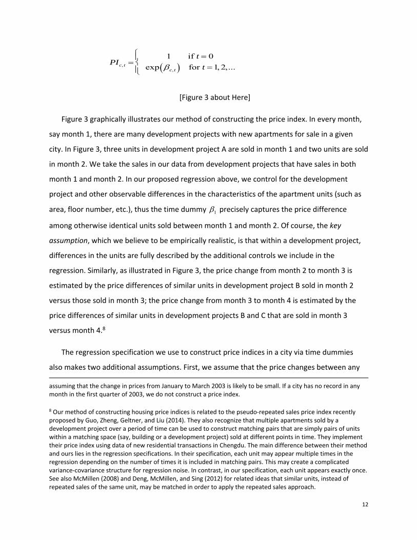
PIc, t
1 if t 0
exp c, t for t 1, 2,...
[Figure 3 about Here]
Figure 3 graphically illustrates our method of constructing the price index. In every month,
say month 1, there are many development projects with new apartments for sale in a given
city. In Figure 3, three units in development project A are sold in month 1 and two units are sold
in month 2. We take the sales in our data from development projects that have sales in both
month 1 and month 2. In our proposed regression above, we control for the development
project and other observable differences in the characteristics of the apartment units (such as
area, floor number, etc.), thus the time dummy precisely captures the price difference
among otherwise identical units sold between month 1 and month 2. Of course, the key
assumption, which we believe to be empirically realistic, is that within a development project,
differences in the units are fully described by the additional controls we include in the
regression. Similarly, as illustrated in Figure 3, the price change from month 2 to month 3 is
estimated by the price differences of similar units in development project B sold in month 2
versus those sold in month 3; the price change from month 3 to month 4 is estimated by the
price differences of similar units in development projects B and C that are sold in month 3
versus month 4.8
The regression specification we use to construct price indices in a city via time dummies
also makes two additional assumptions. First, we assume that the price changes between any assuming that the change in prices from January to March 2003 is likely to be small. If a city has no record in any month in the first quarter of 2003, we do not construct a price index.
8 Our method of constructing housing price indices is related to the pseudo‐repeated sales price index recently proposed by Guo, Zheng, Geltner, and Liu (2014). They also recognize that multiple apartments sold by a development project over a period of time can be used to construct matching pairs that are simply pairs of units within a matching space (say, building or a development project) sold at different points in time. They implement their price index using data of new residential transactions in Chengdu. The main difference between their method and ours lies in the regression specifications. In their specification, each unit may appear multiple times in the regression depending on the number of times it is included in matching pairs. This may create a complicated variance‐covariance structure for regression noise. In contrast, in our specification, each unit appears exactly once. See also McMillen (2008) and Deng, McMillen, and Sing (2012) for related ideas that similar units, instead of repeated sales of the same unit, may be matched in order to apply the repeated sales approach.
1

13
two months are uniform across development projects that may be located in different parts of
the city.9 To see this, note from Figure 3 when we estimate the price change from month 3 to
month 4, we pool the units sold in development projects C and D in the two months in the
regression; since we restrict the time dummy not to interact with the development projects, we
implicitly assume that the price changes in development projects C and D from month 3 to
month 4 are the same. Second, we also implicitly assume that the only source of price changes
between any two months in a development project is the overall change in the housing market
in the city. In particular, we assume that developers do not change their pricing strategies as
new units go on the market.10 One may also be concerned that over time, the amenities and
infrastructure around the development projects may improve and thus part of the price
differences for units in the same development project sold in different months may reflect such
differences, not the housing market conditions. We believe that this is less likely an issue in
China, as buyers of earlier units are almost certainly aware of upcoming improvements in the
infrastructure (e.g. subway stations, shopping malls, etc.) close to the development projects, as
such projects are public information and developers surely advertise them to earlier buyers.
3. The Chinese Housing Market Boom
We use the method outlined in the previous section and a detailed mortgage data set to
construct housing price indices for 120 major cities in China. The list of these cities is given in
Appendix B. Our mortgage data is compiled from mortgage contracts provided by a large
commercial bank, which accounts for about 15 percent of the mortgage loan market in China.
We restrict the sample to mortgages for new, residential properties and as a result have over
9 This assumption in principle can be relaxed. If each month we have a sufficiently large number of sales located in each district of a city, we can implement our regression at the district level and construct district‐specific price indices. As a robustness check, we have divided Beijing into inner region that is close to the town center and suburban area and constructed separate indices for the two areas. The monthly changes of these two indices are highly correlated with a correlation of 0.93, although the index for the inner region grew slightly faster than that for the suburban area during our sample period. 10 It is not clear how developers would change their pricing strategies during the course of sales of units in a project. Wu, Deng, and Liu (2014) provide some evidence from hedonic regressions that the unit prices tend to lower when the percentage of units in the projects already sold is higher. However, as they admitted, this does not necessarily imply that developers are using different pricing policies for units that go on the market in different months.

14
one million mortgage loan contracts dating from the first quarter of 2003 to the first quarter of
2013. A typical mortgage contract contains detailed information on the personal characteristics
of home buyers (e.g., age, gender, marital status, income, work unit, education, occupation,
and region and address of residence), housing price and size, apartment‐level characteristics
(e.g., complex location, floor level, and room number), as well as loan‐level characteristics (e.g.,
maturity and down‐payment).
[Figure 4 about Here]
Based on the transacted home prices and characteristics, we build housing price indices for
120 cities in China from 2003‐2013. As our price indices are nominal, it is useful to keep in mind
that inflation was modest during that decade. Figure 4 depicts the national inflation together
with bank deposit rate. The national inflation fluctuated substantially from low levels around 2
percent in 2003‐2007 to a peak level of 8 percent in early 2008, only to quickly drop to below ‐
1.5 percent in the first half of 2009, rising to around 5 percent in 2011 and eventually returning
to a level around 2 percent in 2013. Inflation had a modest average rate of 2.68 percent during
our sample period. Figure 4 also shows that the bank deposit rate stayed in a narrow range
between 2 and 4 percent during this period.
Our housing price indices allow us to precisely characterize the housing market boom in the
last decade throughout China. We describe the housing market boom below by tiers of cities.
A. First‐Tier Cities
[Figure 5 about Here]
Figure 5 depicts the monthly housing price indices for the four first‐tier cities in four
separate panels, together with measures of households’ purchasing power. In Panel A, the
housing price index of Beijing experienced an enormous rise from an index level of 1 in January
2003 to 7.6 in March 2013. That is, the housing price level has increased 660% in a short period
of ten years!
During this period, Beijing’s housing prices have actually experienced at least two episodes

15
of downward movement. The first episode started in May 2008, when the price index was at
3.50 (relative to January 2003), and continued until March 2009, when the price index slid to
3.05. This represented a 13% price drop and coincided with the global financial crisis. The
second episode is more recent. It began in May 2011 and ended in June 2012 when the housing
price index fluctuated between the interval of 5.99 and 6.67.
As benchmarks for the housing price appreciation, Panel A also plots two measures of the
households’ purchasing power in Beijing: per capita Gross Regional Product (GRP) and
disposable income (urban) during the same period. The per capita GRP measures the per capita
value of output in the whole city and the per capita disposable income (urban) measures the
per capita income received by urban residents of the city. Both of these measures have
experienced similar growth from 1 in 2003 to a level around 3 in 2013. While this growth is
remarkable by any standard, it is nevertheless substantially smaller than the housing price
appreciation in the city.
Panel B plots the monthly housing price index for Shanghai. The index increased from 1 in
January 2003 to about 4.43 in March 2013. The overall housing price appreciation in Shanghai
was more modest than that in Beijing, even though Shanghai’s housing price appreciation
actually started faster than Beijing. Shanghai’s housing prices doubled by April 2005 relative to
that in January 2003, while Beijing’s housing prices did not double until August 2006. However,
Shanghai experienced three episodes of price adjustment in the last decade. The first
adjustment started in May 2005 when the index was at 2.05, and ended in March 2007 when
the index went down to as low as 1.79. This represented a 13% price correction. However, the
housing prices picked up again from March 2007 to reach an index level of 2.72 in August 2008.
The second episode was a swift and small adjustment with the index dropping from 2.72 in
August 2008 to 2.41 in December 2008. The third episode started in June 2011 with the price
index dropping from 4.27 to as low as 3.20 in March 2012. This represented a 25% price
correction. However, housing prices picked up again from March 2012. By March 2013, the
price index reached its peak at 4.43.
The growth of households’ disposable income in Shanghai during this period was about the

16
same as that in Beijing, with disposable income of urban residents roughly tripling from January
2003 to March 2013. Thus, the housing price appreciation in Shanghai, while quite substantial,
is nonetheless much more closely aligned with the growth of disposable income. The other
measure of purchasing power, GRP per capita, exhibits more modest growth in Shanghai, but it
still more than doubled in this period.
Panels C and D respectively plot the housing price indices for Guangzhou and Shenzhen. The
overall picture of these two cities in Guangdong Province (near Hong Kong) is similar.
Guangzhou’s price index increased from 1 in January 2003 to 5.1 in March 2013, while it rose
from 1 to 3.65 in Shenzhen during the same period. Both cities experienced multiple episodes
of price adjustment. The most severe price adjustment occurred in Shenzhen, starting in
October 2007 when its price index was at 2.97 and reaching a trough in January 2009 when the
index was at 1.82. This represented a 39% price correction. At almost the same time, from
November 2007, Guangzhou’s housing prices also started dropping from an index level of 3.08,
and reached a trough of 2.38 in February 2009. This represented a 23% price correction. Both
Guangzhou and Shenzhen are located in the Pearl River delta, the world’s largest
manufacturing export center. The housing price drops in these two cities were clearly related
to the global economic crisis. The fact that our housing price indices for the two cities are able
to capture these crisis‐induced price‐adjustment episodes lends credence to them.
Panels C and D also reveal that the per capita disposable income in Guangzhou nearly
tripled during the same period, while in Shenzhen grew by only 68 percent. Shenzhen’s per
capita disposable income growth was much smaller than the growth of the per capita GRP,
perhaps because Shenzhen had millions of migrant workers, whose outputs were included in
the calculation of the GRP, but not the per capita disposable income for urban residents with
Hukou (i.e., the official city residence registration).
[Table I about Here]
Table 1 reports, by tiers of city, the summary statistics of the housing return, per capita GRP
and per capita Disposable Income (DI). We report these statistics for the whole period from

17
January 2003 through March 2013, as well as for sub‐periods from January 2003 through
December 2007 and from January 2009 through March 2013. We exclude 2008 between the
two sub‐periods to isolate the potential crisis effects. Panel A reports these statistics in nominal
values, and Panel B reports them in real values, after adjusting for the national inflation rate.
To aggregate the price indices for the four first‐tier cities, we construct a price index for the
tier by setting the initial index level of each city to be one at the beginning of a given period and
then taking an equal weighted average of the index levels of these cities for each subsequent
month. The resulting index level represents the value of a housing portfolio constructed from
investing one RMB into the housing index of each city in the first month and keeping the
portfolio composition throughout the subsequent months. We also use the same method to
construct indices for second‐ and third‐tier cities.
Among first‐tier cities, Panel A shows that the nominal housing price index had an average
annual return of 21% from January 2003 to December 2007. Housing prices dropped in 2008.
After January 2009, the housing price index continued to rise, and on average had another
staggering average annual return of 17.7% from January 2009 to March 2013. Over the whole
10‐year period from January 2003 to March 2013, the housing price index for the first‐tier cities
had an average return of 15.9%!
Panel A also reports the nominal growth of two measures of “purchasing power”: per capita
GRP and disposable income. Both measures have increased significantly in the decade, on
average by 9.4% and 9.3% from January 2003 to March 2013. But the housing price
appreciation in first‐tier cities was nearly twice the magnitudes of the increases in the two
measures of purchasing power.
In real values, Panel B shows that the housing return for first‐tier cities averaged 13.1% per
annum, and the two measures of purchasing power grew on average by 6.7% and 6.6% per
year.

18
B. Second‐ and Third‐Tier Cities
[Figure 6 about Here]
Due to the large number of cities in second and third tiers, we cannot separately plot the
housing price index for each city. Instead, we depict the price index for each of the tiers,
together with measures of purchasing power in Figure 6.
In panel A of Figure 6, the housing price appreciation in second‐tier cities is substantial,
though not as breathtaking as that in the first tier cities. Overall, the price index rose from the
base of 1 in January 2003 to 3.92 in March 2013. The price fluctuations are also more modest
compared to those experienced in the individual first‐tier cities, though part of the moderation
in price fluctuation is the result of averaging over 31 second‐tier cities.
A housing price appreciation of 292% in ten years is remarkable by any standard. It is larger
than the magnitude of housing price appreciation during the U.S. housing bubble in 2000s and
is comparable to the price appreciation during the Japanese housing bubble in 1980s. However,
what is more surprising in Panel A is that the housing price appreciation in second tier cities is
very much in accordance to the growth in measures of purchasing power. To the extent we
believe that income growth, or growth in GRP, represents fundamental demand of households
for housing, the housing price appreciation in the second‐tier cities, though enormous,
nonetheless does not appear to have significantly deviated from the increases in households’
purchasing power.
Table 1 reports summary statistics for the 31 second‐tier cities in our sample. During the
decade from 2003 to 2013, the second‐tier cities on average witnessed an average annual
housing return of 13.2% in nominal values and 10.5% in real values. In the same decade, per
capita GRP had an average annual growth rate of 13.4% in nominal values, fully comparable to
the housing return. The average annual growth rate of per capita disposable income for urban
residents was 11.7% in nominal values, which was only slightly smaller than the housing return.
In nominal values, housing prices in the second‐tier cities grew on average by 16.8% per

19
year from January 2003 to December 2007, while the increase was 11.6% from January 2009 to
March 2013. The increases in housing prices in these two sub‐periods are again commensurate
with the corresponding increases in purchasing power, measured by either per capita GRP or
disposable income.
[Figure 7 about Here]
There are substantial variations among the cities. Figure 7 depicts the logarithmic nominal
housing price appreciation for each city in our sample from January 2003 to March 2013, i.e.
ln . Panel A collects all cities in first and second tiers and Panel B collects cities in the third
tier. We choose logarithmic price appreciation so that we can further break down the price
appreciation of each city into two parts, one in 2003‐2007 and the other in 2008‐2013. Among
the first‐ and second‐tier cities, Beijing had the largest price appreciation in 2003‐2013,
followed by Wenzhou (a coastal city of Zhejiang Province known for its vibrant manufacturing
sector) and Nanjing (the capital city of Jiangsu Province). Yinchuan (the capital city of Ningxia
Province in Northwestern China) had the lowest price appreciation that nevertheless amounted
to over 120% during this period, which came mostly from the second half of the period.
We now examine the price appreciation in third‐tier cities. Panel B of Figure 6 depicts the
aggregate price index and measures of purchasing power for the 85 third tier cities in our
sample. A remarkable feature of the plot is that despite the enormous housing price
appreciation in third‐tier cities during the decade, the housing price increase actually lagged the
growth of disposable income. The housing price index slightly more than tripled, increasing
from the base of 1 in January 2003 to 3.13 in March 2013. According to Table 1, the housing
price index had an average return of 10.6% per year in nominal values or 7.9% in real values.
Again there is substantial heterogeneity across third‐tier cities, as shown in Panel B of Figure 7,
with the price appreciation ranging from 0.1 to 1.8 in log scale (or 10% to 500% in percentage
returns) in 2003‐2013. While the price appreciation is positive across all cities in the full period,
several of them, such as Lianyungang and Huangshan, had substantial price drops in 2003‐2007
and recovered the drops in 2008‐2013.

20
The tripling of the housing index of the third‐tier cities is actually below the growth of the
two measures of purchasing power in these cities in the same period. According to Table 1, per
capita GRP grew on average by 15.0% per year in nominal values during this decade, while per
capita disposable income for urban residents grew on average by 11.7% per year. This pattern,
namely, enormous housing price appreciation but nonetheless below the increases in measures
of purchasing power, also holds in the two sub‐periods.
Overall, housing prices across Chinese cities experienced tremendous growth between 2003
and 2013. The housing price appreciation was particularly dramatic in first‐tier cities, rising over
five fold in 2003‐2013 and substantially outpacing the growth of household purchasing power.
The price appreciation in second‐ and third‐tier cities, while remarkable, was matched by
equally impressive growth in household purchasing power during the same period.
C. Other Housing Indices for Chinese Cities
Micro‐based, constant quality housing price indices for Chinese cities are not yet widely
available. The National Bureau of Statistics (NBS) of China reports two widely used official
housing price series. These two series are commonly known as the "NBS 70‐city index" and the
"NBS Average Price Index."11
NBS 70‐City Index. The NBS started to construct quarterly housing price indices for 35
large‐ and medium‐size cities in 1997. Then, it expanded the list to 70 cities and replaced
quarterly indices to monthly ones beginning in July 2005. In the construction of the "NBS 70‐
City Index," technicians from local statistics authorities are sent in each month to sample
housing complexes and collect raw information on housing transaction prices. For each housing
complex sampled by the local statistics authorities, the average transaction price is calculated in
each month and compared with that of the same complex in the previous month. The monthly
11 The full names of the two series are: “Price Indices for Real Estate in 35/70 Large and Medium Sized Cities” and “Average Selling Price of Newly Built Residential Buildings”, respectively.

21
house price change at city level is then calculated as the average, weighted by transaction
volume, of all complexes’ price changes in the corresponding months.12
NBS Average Price Index. NBS also publishes the total floor area and revenue of houses sold
in 35 major cities, from which average prices can be calculated by simply dividing the total price
paid by total floor area of the transacted units in a given month and given city.
As pointed out in Deng, Gyourko, and Wu (2014b), both official series have well‐known
issues and have been widely criticized: the NBS 70‐City Index is remarkably smooth and shows
very little real housing price growth in 70 Chinese cities in the last decade, while the NBS
Average Price Index fails to control for quality, as it does not account for the fact that the newly
transacted units in a given city are gradually moving to the outer‐rings of the city, an important
feature in rapidly expanding Chinese cities.
[Figure 8 about Here]
Figure 8 depicts our housing price index against the two official series for the four first‐tier
cities. Indeed, the NBS 70‐City Index shows little variation in housing prices during the decade
and is thus in sharp contrast to common experiences in these cities. Interestingly, the NBS
Average Price Index exhibits highly synchronized co‐movements with our index across all four
cities. Such co‐movements are re‐assuring as they indicate that our index is capturing similar
fluctuations as the straightforward calculation of average transaction prices. It is also useful to
note that the NBS Average Price Index shows smaller price appreciation than our index across
three of the four cities, which is consistent with the argument that the average price index does
not account for the gradual shift in the location of the transacted housing units.
Wu, Deng, and Liu (2014) have made a notable attempt to construct micro‐based, constant
quality housing price indices for 35 Chinese cities by using data from the so‐called “Real Estate
12 The details of the statistical procedure used in the “NBS 70‐city Index” can be found at http://finance.sina.com.cn/china/hgjj/20110216/14149383333.shtml (in Chinese). To the best of our understanding, the published procedure for constructing the “NBS 70‐City Index” is conceptually similar to our method, though there are some differences in detail: we include all development projects for sale, while the NBS includes only those sampled housing complexes; we control for a list of unit level characteristics, while the NBS obtains the complex level monthly price by dividing total sales revenue in the complex over the total areas.

22
Market Information System" (REMIS) maintained by municipal housing authorities. This data set
contains major attributes of transacted newly built housing units after 2006. They estimated a
hedonic model where, for each city, housing transaction prices (log) are regressed on
observable characteristics of the unit and its apartment complex, and transaction time
dummies, which they use to construct housing price indices. Whether Wu, Deng, and Liu’s
(2014) housing price indices represent the constant‐quality price indices crucially depends on
the extent to which the observed characteristics included in the hedonic price regressions are
exhaustive. Nonetheless, the housing price indices of Wu, Deng, and Liu (2014) find that for the
35 major cities there was a dramatic housing price surge from 2006 to 2010, with an average
appreciation rate substantially higher than the two official housing price indices.13
D. Experiences in Japan and Singapore
[Figure 9 about Here]
Does the experience of the Chinese housing market differ from that of other Asian countries
during the years of their economic miracle? Figure 9 illustrates the experiences in Japan and
Singapore.
We cannot find a suitable housing price index for Japan going back to the 1960s and 1970s,
which was the period of Japan's rapid economic growth. Instead, Panel A of Figure 9 depicts an
index of urban land price provided by the Japan Real Estate Institute, from 1955 to 2014,
together with the per capita GDP of Japan. Both series are in nominal values and are
normalized to 1 in 1955. From 1955 to 1990, the per capita GDP grew from a level of 1 to about
40, representing an average growth rate of 10.5% per year. In contrast, the urban land price
index grew from 1 to over 80 during the same period, substantially outpacing the per capita
GDP. The Japanese economy has staggered since 1990, with the per capita GDP staying flat for
13 Furthermore, Deng, Gyourko, and Wu (2014a) have constructed a constant‐quality, residential land price index, which they refer to as the “Chinese Residential Land Price Index,” based on similar hedonic regressions, using sales prices of leasehold estates to private developers for 35 major Chinese cities. Their land price index showed extremely high real land price growth across these cities, much more so and with much more cross‐city variations than the “China Urban Land Price Dynamic Monitor” system provided by the Ministry of Land and Resources of China for the same cities.

23
the past 25 years. During this period, the urban land price index continued to fall by half and
eventually converged back to the same level of the per capita GDP in 2014. The dramatic
divergence of the land price index from the per capita GDP before 1990 and the subsequent
convergence vividly illustrates the widely recognized Japanese housing bubble. Based on our
earlier discussion, the housing price appreciation across Chinese cities during 2003‐2013 was
rather different from the experience of the Japanese housing bubble. Except the few first‐tier
cities, the housing price appreciation in the large number of second‐ and third‐tier cities was
largely in line with the growth of household purchasing power.
Panel B of Figure 9 depicts the private property resale price index for Singapore, which is
provided by the Urban Redevelopment Authority of Singapore, together with the per capita
GDP of Singapore, from 1975 to 2010. Both series are in nominal values and are normalized to 1
in 1975. During this period, the per capita GDP grew from a level of 1 to slightly over 10,
representing an average growth rate of 6.6% per year. Interestingly, the housing price index
also grew from 1 to about 11, roughly in line with the GDP growth. While the housing price
appreciation was well matched with the GDP growth for the full period from 1975 to 2010, the
housing price index did diverge substantially from the GDP in two episodes, one in the early
1980s and the other in 1995‐1997, right before the Asian financial crisis. Both episodes
happened after a long period of steady economic growth, during which the housing price index
rapidly appreciated in a few years, significantly outpacing GDP growth. When the GDP growth
slowed, the housing price index collapsed and returned to the level in line with the GDP in a few
years. These price corrections appear very relevant for thinking about potential risk in the
Chinese housing market, especially in the first‐tier cities.
4. Mortgage Borrowers
It is possible to explain the dramatic housing price appreciation in first‐tier cities by the
limited housing supplies in these over‐crowded metropolitan areas. As discussed in Section 1,
the total area of newly completed residential housing in first‐tier cities has substantially slowed
since 2005, while that of second‐ and third‐tier cities has been steadily growing. However,

24
supply is not the only factor that matters to housing markets. As the rising housing prices
directly impact every household in the cities, it is important to fully understand the financial
burdens faced by home buyers, especially low‐income home buyers.
Our detailed mortgage data allow us to provide a comprehensive picture of mortgage
borrowers in different cities, who take loans to buy homes. In this section, we summarize a set
of characteristics of these mortgage borrowers, including household income, down payment,
price‐to‐income ratio, home size, age, and marital status. In particular, we focus on discussing
the financial burdens faced by these mortgage borrowers.
Note that households in the most wealthy fraction of the population may purchase homes
using cash and thus do not appear in our mortgage data. For this reason, our mortgage data is
particularly useful for analyzing the characteristics of relatively low‐income home buyers as
opposed to that of high‐income buyers. We focus on analyzing two sets of borrowers in each
tier of cities: The first set has household income in the bottom 10% among all mortgage
borrowers in a given city and a given year. We refer to this set as the bottom‐income borrower
group. We also denote borrowers with income exactly at the 10 percentile of all borrowers by
p10. The second set has household income in the middle range, specifically within the 45th and
55th percentile of all mortgage borrowers in a given city and a given year. We refer to this set
the middle‐income group and denote borrowers with exactly the median income of all
borrowers by p50.
A. Household Income
[Figure 10 about Here]
Figure 10 depicts the time‐series of the household income of p10 and p50 for first‐, second‐
and third‐tier cities in Panels A, B, and C, respectively. In panels A and B, the left plot shows the
annual income of p10 and p50 (which is averaged across all cities in the tier) in RMB from 2003‐
2012, and the right plot shows the position of p10 and p50 in the income distribution of the city
population based on the income distribution constructed from the Urban Household Survey

25
(UHS). As income distribution is not available for third‐tier cities, Panel C shows only the annual
income of p10 and p50.
Figure 10 shows steady growth in the household income of both p10 and p50 across the
three tiers of cities. In first‐tier cities, the annual household income of p10 grew from 39,000
RMB in 2003 to 92,000 in 2012 while the income of p50 grew from 87,000 in 2003 to 184,000 in
2012. In second‐tier cities, the annual income of p10 grew from 19,000 RMB in 2003 to 58,000
in 2012, while that of p50 from 40,000 in 2003 to 99,000 in 2012. In third‐tier cities, the income
of p10 grew from 15,000 to 51,000, while that of p50 grew from 28,000 to 83,000. This
tremendous income growth of mortgage borrowers is largely consistent with the income
growth of the overall urban population we discussed above.
For most of the first‐ and second‐tier cities, the UHS provides income distribution of urban
households. To specifically compare the income growth of mortgage borrowers with that of the
urban population, we mark the position of p10 and p50 in the population income distribution
reported by the UHS. As our data from the UHS cover only 2003‐2009, we extrapolate the
income distribution in 2009 into the subsequent years based on the city’s average income
growth.
The median‐income borrower p50 came from the relatively wealthy fraction of the
population. In first‐tier cities, p50 declined from the 85th percentile of the population in 2003
to the 59th percentile in 2009 and then climbed back to the 75th percentile. In second‐tier
cities, p50 declined from the 81.5th percentile in 2003 to the 62th percentile in 2010 and then
climbed back to the 68th percentile in 2012.
The position of the low‐income mortgage borrower p10 is particularly interesting. It
indicates the extent to which low‐income households in the population were participating in
the housing markets. Overall, p10 was located at a position around the 25th percentile of the
population in first‐tier cities and around the 30th percentile in second‐tier cities. These
positions indicate that mortgage borrowers were not just coming from the top‐income
households and instead were reasonably well represented in the low‐income fraction of the
population.

26
Interestingly, despite the rapid housing price appreciation in first‐tier cities, p10 steadily
declined from a position around the 35th percentile in 2003 to the 17.5th percentile in 2010
before it climbed back to the 26th percentile in 2012. This suggests that the rapidly growing
prices in recent years have not prevented households from the low‐income fraction of the
population from buying homes. In second‐tier cities, p10 stayed in a range between the 28th
and 40th percentile‐‐‐it declined from a peak of the 40th percentile in 2005 to the 28.5th
percentile in 2010 and then climbed back to the 35th percentile in 2012.
Taken together, Figure 10 shows steady increases in the household income of bottom‐ and
middle‐income mortgage borrowers across the three tiers of cities. Furthermore, despite the
tremendous housing price appreciation in these cities, mortgage borrowers were well
represented in the population and the housing market participation of households from the
low‐income fraction of the population remained stable.
B. Down Payment
Mortgage down payment is a key variable that determines the leverage used by mortgage
borrowers and serves as an equity buffer to prevent borrowers from defaulting on the loans in
the event of a future housing price meltdown. Figure 11 depicts the fraction of down payment
in the home value at the time of purchase, separately for the bottom‐ and middle‐income
groups.
[Figure 11 about Here]
The right panel shows that for mortgage borrowers in the middle‐income group, down
payment on average contributed to at least 35% of home value across the three tiers of cities.
Interestingly, the left panel shows that for borrowers in the bottom‐income group, the fraction
of down payment was even higher‐‐‐it was consistently above 38% across the three tiers of
cities.
These high levels of down payment are consistent with the strict mortgage policies imposed
by the Chinese government on banks. Specifically, the policies restrict one housing unit from
being used as collateral for more than one mortgage loan. The policies also require a minimum

27
down payment of 30% on first mortgages. As detailed in Appendix A, this minimum down
payment requirement had changed over time between two levels: 30% or 40%. Banks have
requested even higher down payments on second mortgages that are used to finance
purchases of second homes.
The high levels of mortgage down payment used by Chinese borrowers were in sharp
contrast to the popular use of zero down payment loans and negative amortization loans during
the U.S. housing bubble of 2000s. According to Mayer, Pence, and Sherlund (2009), during the
U.S. housing bubble period of 2003‐2006, households with poor credit (the so‐called subprime
and Alt‐A households) had commonly used mortgages with a 5% or zero down payments to
finance their home purchases. Some mortgages even allowed the borrowers to have negative
amortization over time. When the U.S. housing prices started to decline after 2006, these
borrowers were more likely to default on their mortgage loans, exacerbating the housing
market decline. The high levels of down payments used by households throughout China
mitigated the risk of household default in the event of a future housing market meltdown.
Unless the housing prices decline by over 30%, the mortgage borrowers are unlikely to default
on their loans. 14 Furthermore, mortgage loans in China are all recourse loans, which allow
lenders to collect borrowers’ other assets in the event of mortgage defaults. These reasons
make a U.S. style subprime credit crisis less of a concern for China.
C. Price‐to‐Income Ratio
[Figure 12 about Here]
Price‐to‐income ratio provides a convenient measure of the financial burdens endured by a
household in acquiring a home. Figure 12 depicts the price‐to‐income ratio of mortgage
borrowers in the full sample (top panel) and in the subsample of married borrowers (bottom
panel). In each panel, there are two plots, the left plot covers the borrowers in the bottom‐
14 According to annual reports of the China Banking Regulatory Commission (CBRC), the ratio of non‐performing loans in residential mortgages has remained below 0.6% since 2009. Even in Shenzhen, which, as we discussed earlier, experienced a large housing price drop of 39% in 2008, the ratio of non‐performing loans in our sample remained lower than 1.5% in 2008.
28
income group with a separate line for each of the three tiers of cities, while the right plot covers
the borrowers in the middle‐income group.
The financial burdens faced by the bottom‐income group are particularly interesting. In this
group, the price‐to‐income ratio started at a level slightly above 8 across the three tiers of cities
in 2003. In first‐tier cities, this ratio remained at around 8 before 2008 and then climbed to a
peak of 10.7 in 2011 before dropping back to 9.2 in 2012. In second‐ and third‐tier cities, this
ratio was very similar and remained in a tight range around 8. It had a modest decline from a
level slightly above 8 in 2003 to 7.2 in 2007 and then climbed back to a peak slightly below 9 in
2011 before dropping back to around 8 again.
The price‐to‐income ratio for the middle‐income group was consistently lower than that for
the bottom‐income group. It was highest in the first‐tier cities and lowest in the third‐tier cities.
Across the three tiers of cities, it had a similar pattern over time. In first‐tier cities, it had an
expansion from 5.6 in 2003 to 8.3 in 2011 before dropping back to 7.5 in 2012. In second‐tier
cities, it expanded from 5.7 in 2003 to 7.4 in 2010 before dropping back to 6.2 in 2012. In third‐
tier cities, it expanded from 5.0 in 2003 to 6.4 in 2010 before dropping back to 6.2 in 2012.
It is useful to compare the price‐to‐income ratios observed in Chinese cities with that in
other countries. Cheng, Raina, and Xiong (2014, Table 9) examined home purchases by Wall
Street employees and lawyers in the U.S. during 2000s and found that they had consistently
used price‐to‐income ratios around three before, during, and after the U.S. housing bubble that
peaked in 2006. While the households they examined were from the relatively high‐income
fraction of the U.S. population, it is common for financial advisors in the U.S. to advise
households to purchase homes with price‐to‐income ratios of around three.15 There are few
studies of financial burdens faced by mortgage borrowers during the Japanese housing bubble.
Indirectly, Noguchi (1991, Table 1.3) reported that the average ratio of condominium price (the
price of a certain benchmark condominium) to annual income, i.e., the income of an average
15 The lack of property taxes in China has contributed to the high price‐to‐income ratio observed in China relative to that in the U.S. It is common for homeowners in the U.S. to pay annual property taxes in the range of 1‐2% of home values to local townships, while home owners in China typically do not pay any property tax.

29
household which may or may not be a home buyer, in Tokyo rose to 8.6 in 1989, which is
consistent with the price‐to‐income ratios used by the bottom‐income borrowers in China.
A price‐to‐income ratio of 8 or higher, which had been commonly used by mortgage
borrowers in the bottom‐income group throughout the Chinese cities, implies substantial
financial burdens on the borrowers. The financial burdens are reflected in several dimensions.
First, in order to qualify for a mortgage loan, a borrower needs to make a down payment of
about 38% of the home value (Figure 12), which is equivalent to about three times of the
borrower’s annual income. This large down payment would require many years of saving. In
practice, many home buyers, who are typically in their early 30s (as we will show below), rely
on savings of their parents or other close family members to make the down payment.16
Second, monthly mortgage payments also consume a substantial fraction of the household
income. To illustrate this burden, consider a household, which bought a home at a price that
was eight times of its annual disposable income. Suppose that it used its saving to make the
down payment at three times its annual income and took a mortgage loan that was five times
its annual income. As we describe in Appendix A, all mortgage loans in China carry floating rate
interest payments, with the rate determined by a benchmark lending rate set by the People’s
Bank of China. If the annual mortgage rate was 6%, a rather low rate relative to the rate
observed in recent years, then the annual interest payment would consume 6% 5 30% of
the household’s annual income. Furthermore, the household also needed to pay back a fraction
of the mortgage each year. Suppose that the loan had a maturity of 30 years (maximum
maturity allowed in China) and linear amortization. Then, the household had to set aside
another 16.7% of its annual income to pay the mortgage. Together, servicing the
mortgage loan would consume 46.7% of its annual income.
As we will discuss later, a significant fraction of home buyers in the bottom‐income group
were unmarried. As they would eventually get married and as it is common in China for a
16 Due to the high savings rates by Chinese households and the Chinese tradition of children supporting parents in their old age, parents are usually able and willing to provide some financial support to their children’s home purchases. For this reason, there is typically not another hidden loan (i.e., a loan taken through the shadow banking system) to pay for the down payment.

30
married couple to both work, the household income of a single buyer may soon double upon
his/her marriage. Then, the price‐to‐income ratio of single buyers may not accurately reflect
their financial burdens. To isolate this issue, we also compute the price‐to‐income ratio of
married couples in the bottom‐income and middle‐income groups in each tier of cities. The
bottom panel of Figure 12 shows that the price‐to‐income ratio of married borrowers was very
similar to that of the full sample with both married and unmarried borrowers across both
income groups and different tiers of cities. This lack of difference may reflect the fact that
Chinese banks follow a rigid system of using current household income to determine the
amount of mortgage loans available to borrowers, regardless of their marital status.
The remarkable income growth of Chinese households during this decade also implies that
the large financial burdens endured by mortgage borrowers might be temporary and would
subside over time as their income grew. Again consider the household, which purchased a
home at an initial price‐to‐income ratio of eight. Suppose that the household expected its
income to grow at an annual rate of 10%, which was roughly the growth rate during this period.
Then, it expected its income would rise to 1.6 times of its initial level in five years; the ratio of
the current home price to its future income in five years would be five. Of course, this
calculation depends on a crucial assumption that the 10% income growth rate would persist
into the future. This assumption is ex ante strong despite that ex post the household income in
China has been growing at this impressive rate for three decades.
Nevertheless, this simple calculation shows that the household’s expected income growth
rate is crucial for determining how much it is willing to pay for a home relative its current
income. If the household expected its income to persistently grow at a high rate, it would
expect the large financial burdens brought by buying a home at eight times of its current annual
income to be temporary. Furthermore, this expectation might also motivate an expectation
about high income growth of other households, which may in turn lead to an expectation that
housing prices will continue to rise. Such an expectation further motivates the household to
take on enormous financial burdens to buy the home. In this sense, the households’
31
expectations about their income growth and future housing price appreciation are central for
understanding the housing market boom. We will return to this issue in our later discussion.
D. Home Size
[Figure 13 about Here]
Home size is an important dimension for determining the consumption value of a home.
Figure 13 depicts the size of the homes purchased by bottom‐income and middle‐income
mortgage borrowers across the three tiers of cities. Despite the large financial burdens endured
by the mortgage borrowers, their homes were rather spacious. The bottom‐income borrowers
in first‐tier cities, which are the most expensive cities in China, bought the smallest homes in
our sample. Even for these borrowers, the average size of their home was in a range between
72 and 80 square meters throughout the decade. For a typical family of three (a couple with
one child based on China’s birth control policy), this home size implies about 25 square meters
per person, which is quite spacious by the standards of most large metropolitan areas in the
world such as Hong Kong, New York, Singapore, and Tokyo.
It is also useful to note the evident declining trend in the home size purchased by all groups
in the three tiers of cities. The homes purchased by bottom‐income borrowers in second‐tier
cities on average declined from 90 square meters in 2003 to 80 in 2012, while the homes
purchased by bottom‐income borrowers in third‐tier cities declined from 109 square meters in
2004 to slightly above 90 in 2012. The homes purchased by middle‐income borrowers tended
to be bigger but also had a similar decline across all three tiers of cities.
E. Age and Marital Status
[Figure 14 about Here]
Figure 14 shows the age of mortgage borrowers in our sample. Across the three tiers of
cities, the mortgage borrowers were on average in their early 30s. The borrowers in the
bottom‐income group tended to be slightly younger than those in the middle‐income group.
[Figure 15 about Here]
32
A significant fraction of the borrowers are unmarried. Figure 15 summarizes the fractions of
single men and single women among the mortgage borrowers in each income group and each
tier of cities. Single men and single women contributed to at least 40% of the bottom‐income
mortgage borrowers across the three tiers of cities in each of the years from 2003‐2012. This
fraction was lower among the middle‐income borrowers but nevertheless substantial.
Wei, Zhang, and Liu (2014) argue that home ownership is a status good for single men to
strengthen their competitiveness in the marriage market due to the widespread sex imbalance
in China. This argument implies that single men should be more eager to buy homes than single
women. Consistent with this argument, the fraction of single men among mortgage borrowers
was consistently higher than the fraction of single women in second‐ and third‐tier cities across
all years and across the bottom‐income and middle‐income borrower groups. However, in first‐
tier cities, the fraction of single men was roughly the same as the fraction of single women
among the middle‐income borrowers, and the fraction of single men was even lower than the
fraction of single women among the bottom‐income borrowers throughout the sample
period.17 This suggests that while marriage market competition might be a determinant of
home ownership in second‐ and third‐tier cities, it is not as relevant for understanding the
particularly high housing prices in first‐tier cities.
F. Second Mortgages
An often discussed concern regarding the Chinese housing markets is that many urban
households hold multiple homes and leave a significant fraction of homes vacant for prolonged
periods of time. Our mortgage data allow us to separate second mortgages (i.e., mortgage
loans taken by households to purchase second homes) from first mortgages (i.e., single
mortgages taken by households) after 2010.18
[Table 2 about Here]
17 This pattern is consistent with casual observations that sex imbalance is less severe in first‐tier cities as people in these cities have been more open‐minded about having girls and thus less prone to selecting the sex of their children. 18 As we explain in Section 6, in early 2010 the Chinese government raised the down‐payment ratio and the interest rate on second mortgages, making them higher than those for first mortgages. Since then, banks need to collect information about whether each mortgage is a first or second.

33
Table 2 summarizes the fraction of second mortgages among all mortgage loans issued in
each tier of cities in each year between 2011 and 2013. This fraction offers a measure of the
extent that households took loans to buy investment homes. As wealthy households may
simply use cash to buy investment homes, such investment purchases by wealthy households
do not appear in our mortgage data. Thus, the fraction of second mortgages underestimates
the home purchases driven by investment demands.
In first‐tier cities, the fraction of second mortgages was 5.3% and 5.2% in 2011 and 2012,
respectively, and this fraction had a dramatic increase to 11.8% in 2013. In second‐ and third‐
tier cities, the fraction of second mortgages also had an increasing trend during this period,
although the levels were much lower. In second‐tier cities, this fraction grew from 2.0% in 2011
to 2.4% in 2012 and 3.3% in 2013. In third‐tier cities, it grew from 1.0% in 2011 to 1.3% in 2012
and 1.8% in 2013. Taken together, mortgage‐financed investment home purchases were much
more pervasive in first‐tier cities than in second‐ and third‐tier cities.19
In summary, our analysis of the mortgage data shows that despite the enormous housing
price appreciation during the last decade, the participation of low‐income households in the
housing markets remained steady. Nevertheless, the relatively low‐income home buyers
endured severe financial burdens in order to buy homes at prices commonly over eight times
their current income. This behavior reflected expectations of persistently high income growth
and further high housing price appreciation.
5. Housing as an Investment Vehicle
The spectacular economic growth of China since the 1980s has been accompanied by a high
savings rate. According to Yang, Zhang, and Zhou (2013), the gross national savings as a
percentage of GDP averaged 35% during the 1980s, 41% during the 1990s, and surged to over
19 The fraction of second mortgages in our mortgage data may appear substantially lower than the fraction of households owning multiple homes reported by Chinese Household Finance Survey (2012). According to this survey conducted in 2012, the fraction of urban households owning at least two apartments in China is 15.44%. Note that a significant fraction of the multiple homes owned by the surveyed households was probably old‐style housing units that were assigned to the households by their employers as in‐kind compensation before the housing reform in late 1990s. These units tended to have undesirable qualities and were different from the newly built homes‐‐the typical homes bought by households in recent years.

34
50% in the 2000s. This high saving rate surpassed the rates of all major countries during the
same period and was also higher than the prevailing rates in Japan, South Korea, and other East
Asian economies during the years of their miracle growth. Households, firms, and the
government have all contributed to the remarkably high savings rate in China. Savings by
households and firms had each reached about 20% of the GDP during the 2000s.
Despite the high savings rate, households and firms in China have limited vehicles in which
to invest their massive savings. Bank deposit accounts are the predominant investment vehicle
in China. Due to China's restrictive capital controls, households and firms cannot freely invest
their savings in capital markets outside of China, and although they can invest in the stock
market inside China, it is still small by size relative to the pool of savings and has not offered
attractive returns in the last two decades.20 Bond markets in China are even smaller. Given
these limited investment choices, Chinese households often use housing as an alternative
investment vehicle. In this section, we discuss the performance of housing as an investment
vehicle, in comparison to bank deposits and stock market.
A. Bank Deposits
[Figure 16 about Here]
Figure 16 shows that total bank deposits in China rose from slightly above 20 trillion RMB in
2003 to over 100 trillion in 2013. The deposit rate is regulated by the central bank. As shown in
Figure 4, the nominal bank deposit rate remained in a narrow range, between 2 and 4 percent
in 2003‐2013, while the national inflation rate frequently surpassed the nominal deposit rate in
2004, 2008‐2009, and 2011‐2012, making the real deposit rate negative. The average real
deposit rate in 2003‐2013 was 0.01 percent. This low deposit rate makes the huge pool of bank
deposits rather striking. Nevertheless, the low deposit rate has motivated Chinese households
to search for alternative vehicles to invest their massive savings.
20 There is a debate regarding the performance of the Chinese stock market. On one hand, Allen, et al (2014) argue that despite China's spectacular economic growth, the Chinese stock market has performed rather poorly. On the other hand, Carpenter, Lu and Whitelaw (2014) argue that the Chinese stock market has become as informative about future corporate profits as the U.S. stock market.

35
B. Stocks
China established two stock exchanges in the early 1990s, one in Shanghai and the other in
Shenzhen. Figure 16 shows that the market capitalization of all floating shares in the stock
market grew from less than 2 trillion RMB in 2003 to near 20 trillion in 2013. Despite this rapid
expansion, the size of the stock market was still substantially smaller than the total bank
deposits.
[Figure 17 about Here]
Figure 17 depicts the Shanghai Stock Market Index, a widely followed index for the Chinese
stock market, for 2003‐2013. This period witnessed a dramatic stock market boom and bust in
2006‐2008, when the index rose from 1200 at the beginning of 2006 to a peak of 6092 in
October 2007 and then plunged to just below 2000 in October 2008. This boom and bust cycle
mostly coincided with the rise and fall of stock markets all over the world in conjunction with
the financial crisis in 2008. Since 2008, the Shanghai Stock Market Index recovered in 2009 to a
level slightly above 3000, but declined again after 2010 to a level around 2000.
[Table 3 about Here]
Table 3 summarizes the risk and return from investing in the Shanghai Stock Market Index in
2003‐2013. During this period, its annual return was an average of 7.3% and it had volatility of
51.5%. This high volatility is not surprising given the dramatic stock market boom and bust in
2006‐2008. To isolate this boom and bust period, Table 3 also splits the sample into two sub‐
periods. In the first half (2003‐2008), despite the market crash in 2008, the index return had an
average of 8.98% and a staggering volatility of 66.1%. In the second half (2009‐2013), the index
return had an average of 5.3% and a volatility of 33.9%.
C. Housing
[Table 4 about Here]
Table 4 summarizes the annual returns of the housing indices of first‐, second‐, and third‐
tier cities. During our full sample in 2003‐2013, first‐tier cities offered the highest average

36
annual return at a staggering level of 15.7% and return volatility of 15.4%, second‐tier cities
offered an average return of 13.4% and volatility of 9.9%, while third tier cities offered the
lowest average return of 11.0% among the three tiers and also the lowest volatility of 7.5%.
Relative to the stock index return in the same period, the housing indices across the three tiers
all offered higher average returns and, more impressively, much lower volatility. Despite the
economic turmoil after 2008, the volatility of housing returns had been remarkably low.
During the first half of the sample, 2003‐2008, the housing returns were particularly high for
first‐ and second‐tier cities, with the first‐tier housing index offering an average return of 20.4%
and the second‐tier 17.3%. During the second half of the sample, 2009‐2013, average returns of
both the first‐and second‐tier were lower at 10.9% and 9.7%, which are nevertheless attractive
relative to the average stock index return during the same period. The index return of third‐tier
cities was stable across the two sub‐samples at 11.7% and 10.3%, respectively.
Overall, the housing returns from all three tiers of Chinese cities were surprisingly resilient
across the economic crisis period of 2008‐2009 and offered returns substantially more
attractive than bank deposits and the Chinese stock market.
6. Discussion
Our analysis provides some basic facts to allow us to understand and interpret the Chinese
housing boom. In this section, we offer discussion based on these facts.
Housing booms are often associated with credit expansions, with the recent housing bubble
in the U.S. being a vivid example. As a result, commentators have often been concerned by the
potential risk of excessive leverage in driving the Chinese housing boom. As we have described
earlier, Chinese banks have required down payments of over 30 percent for all mortgage loans.
Such high down payment ratios substantially alleviate the household default risk faced by banks
and make reckless credit expansions to households an unlikely cause of the Chinese housing
boom.

37
A particular concern about the Chinese housing boom is that the enormous housing price
appreciation across Chinese cities might constitute a housing bubble that is about to burst. As is
well known by economists, it is difficult to reliably identify an asset bubble. There may or may
not be a housing bubble in the Chinese housing market. To forcefully determine the presence of
a housing bubble, one needs to develop a systematic framework of supply and demand of
housing that fully accounts for the growth of the Chinese economy and the frictions in the
Chinese financial system. This entails a task substantially more ambitious than the goal of this
paper. Nevertheless, our analysis offers some useful observations about the nature of this
nationwide housing boom.
On one hand, the enormous price appreciation does not necessarily indicate the presence
of a bubble, as the price appreciation has been mostly accompanied by equally impressive
household income growth, except in a few first‐tier cities. On the other hand, housing prices
are indeed expensive relative to the income of many households, in particular, of the low‐
income mortgage borrowers. While one can justify their willingness, despite the severe
financial burdens, to buy homes based on expectations of persistently high income growth, the
high price‐to‐income ratios observed across Chinese cities expose the housing market to
substantial risks when households’ expectations are subdued in the future, especially in the
event of a sudden stop in the Chinese economy.
Our analysis also highlights a few key ingredients for future efforts to develop a systematic
framework for analyzing the Chinese housing market:
1. The housing market across first‐, second‐, and third‐tier cities offered high returns,
substantially more attractive than bank deposits and the Chinese stock market.
2. Housing price levels were also high across the three tiers of cities with low‐income
households buying homes at prices that were over eight times their annual income.
3. Concurrent with the housing boom, Chinese households also accumulated a large pool
of cash in bank deposits that paid a minimal deposit rate.

38
It is important to fully account for the distortions brought to the housing market by the
imperfections in the Chinese financial system. The low bank deposit rate that had persisted
throughout the studied decade is a key factor. To the extent that near 100 trillion RMB has
been sitting in bank deposits earning an almost zero real rate, households’ investment demand
for housing is an important driver of housing prices in China.21
Beside the well‐known illiquidity of housing, risk is an important dimension in evaluating
housing as an investment asset. It is difficult to measure the crash risk of the housing market
based on month‐to‐month price fluctuations. The housing market was rather resilient across
the crisis period of 2008‐2009. In this regard, the housing market has been more robust to
crash risk, relative to the stock market, even though the low risk experienced by the housing
market in the past does not necessarily imply low risk going forward. As discussed by Pritchett
and Summers (2014), the spectacular growth rate of the Chinese economy during the last three
decades is clearly a rare event and the powerful force of regression to the mean would make a
continued high growth rate of 9 or even 7 or 6 percent an even more unlikely event. This
argument implies a substantial risk of an eventual economic slowdown. To the extent that low‐
income households were buying homes by enduring substantial financial burdens, the risk
perceived by them was unlikely to be large. Thus, a systematic framework needs to account for
the expectations of households, in particular, their optimistic expectations about persistently
high growth rates into the future.22
It is also useful to note that housing demand may also be driven by reasons beyond
consumption and investment needs. Wei, Zhang, and Liu (2014) emphasize the role of housing
as a status good, which strengthens the competitiveness of unmarried men in an unbalanced
marriage market where men substantially outnumber women. Indeed, our analysis also
21 Chen and Wen (2014) derive a theory to explain the persistently faster‐than‐GDP housing price growth during the Chinese housing boom based on an idea that a self‐fulfilling housing bubble can induce productive entrepreneurs to divert capital from profitable investment projects in order to speculate in housing. 22 Zheng, Sun, and Kahn (2014) build a measure of real estate confidence level for 35 Chinese cities by using Internet search data. They show that this index predicts subsequent housing price appreciation and new housing construction.

39
confirms relatively larger fractions of unmarried men to unmarried women among mortgage
borrowers in second‐ and third‐tier cities, albeit not in first‐tier cities.
While our analysis has been largely focused on the demand side of the housing market, the
supply side is equally important. There is still a lack of systematic understanding of housing
supply in Chinese cities. To the extent that housing prices have been rising at a pace
comparable to or even higher than the households’ income growth rate during the decade, the
housing market equilibrium implies that the growth of housing supply was likely to have stayed
either below or comparable to the growth of housing demand, even though Deng, Gyourko,
and Wu (2014b) document some evidence of a large housing inventory held by developers in
several major cities in recent years. Different from U.S. cities where housing supply is often
determined by landscape and local zoning restrictions, e.g., Saiz (2010), housing supply in
Chinese cities is determined by land sold by local governments for housing development, as
land is legally owned by the state and controlled by local governments. As we will discuss in the
next section, land sale revenues have contributed to a substantial fraction of local governments’
fiscal budget. As a local monopoly of land supply, local governments’ land sales strategy is a key
factor in determining housing prices in Chinese cities.
7. Roles of Government in the Housing Market
In China, the governments at the central and local levels have been actively engaged in the
housing market. The powerful forces induced by government policies not only directly affect
physical aspects of the housing market such as supply of land and availability of funds to buyers,
but also delicately influence expectations and confidence of households about the housing
market. This is an important channel for understanding the drastically divergent performance
of the housing and stock markets after 2008. In this section, we briefly discuss the role of
government in the housing market, first on the policy interventions of the central government
and then on the dependence of local governments on land sales for their fiscal revenues.
A. Interventions by the Central Government

40
By 2007, housing prices in most Chinese cities had grown substantially, as discussed in
Section 3. In response, the central government implemented a series of monetary and fiscal
policies to curb soaring prices and curtail speculative activities in the housing market. For
example, in September 2007, the central government raised the minimum down payment ratio
from 30 percent to 40 percent, raised the interest rate on second mortgages to 10 percent
higher than the benchmark rate, and capped the monthly mortgage payment‐to‐income ratio
at 50%. In April 2008, it imposed tax on capital gains from housing sales. The government also
started to increase the construction of government‐subsidized housing, such as affordable
housing, low‐cost housing, and public rental housing, to help relieve the pressure on the
housing market.
These policies might have had some effects on housing prices, especially in cities in
Guangzhou and Shenzhen during this period, though it is hard to distinguish the effects of the
policies from that of the emerging global economic crisis. In any event, in October 2008 the
central government abruptly reversed these policies, and installed a series of measures to
support housing market recovery. It reduced the minimum mortgage rates to 70 percent of the
benchmark rate and the down‐payment ratio to 30 percent. As part of its 4 trillion RMB
stimulus package, it also designated the real estate sector as one of the primary industries for
investment. As a result, the housing market regained momentum in mid‐2009 and started a
new round of rapid price appreciation.
In early 2010, the government introduced a series of measures, some traditional and some
less standard, to cool off what were widely considered a once again overheating housing
market. It again raised the down‐payment ratio to 40% and the interest rate on second
mortgages. More important, starting in April 2010, following the guidelines of the central
government, 39 of the 70 major cities in China introduced the housing purchase restriction
policies.23 Under these policies, only those with local Hukou (household registration), or those
23 The housing purchase restriction policy was initiated by the central government under the so‐called “New National Ten Articles” and “New National Eight Articles” issued in April 2010 and January 2011 respectively, which provided guidelines saying that housing purchase restrictions should be implemented in first‐tier cities and could be extended to second‐ and even third‐tier cities on an as‐needed basis. In Beijing, for example, the policy requires that only a household with household registration in Beijing can buy a new apartment. Migrants living in

41
who could show proof of employment in the city for certain consecutive years, were eligible for
purchasing one or two new homes. Though not covered in our sample period, the slowdown in
the Chinese economy has led to a slowdown of the residential housing market since the end of
2013. Many cities loosened the purchase restrictions in mid‐ 2014. Currently, the housing
purchase restriction policies are in force only in the four first‐tier cities.
The frequent interventions by the central government have created a sense among the
households that the housing market is too important to fall, as whenever the market started to
fall, the central government would provide supports to sustain it.
B. Land Sales and Fiscal Revenue of Local Governments
Land sale revenues have contributed to a substantial fraction of local governments’ budgets.
This feature was a result of the fiscal reforms enacted in 1994. In the reforms, the central
government consolidated provisions for tax revenue collection and sharing in order to
redistribute tax revenues to less developed areas. As is well known, local officials in China were
evaluated for promotion based to a large extent on regional economic growth (Li and Zhou,
2005), which provided strong incentives for investment in infrastructure and capital projects.
However, unlike local governments in western countries, local Chinese governments do not
have many sources of revenue. In particular, local governments in China are not authorized to
levy sales taxes, property taxes, or local income taxes, which are important sources of revenue
for local governments in western countries. Moreover, local governments in China are
prevented from directly issuing debt to fund capital projects.
[Figure 18 about Here]
As a result of this central/local fiscal arrangement and the restrictions placed on local
governments, China has developed a unique source for local governments to obtain capital
necessary to fund required large‐scale infrastructure investments‐‐‐they increasingly rely on
selling public land. Figure 18 shows the share of land revenues in city fiscal budgets from 2003‐
Beijing are not allowed to buy any apartment unless they can provide documentation to prove payment of taxes and social security contributions for the previous five consecutive years. Shanghai’s policy is similar.

42
2011 averaged across all cities, as well as among the first‐tier, second‐tier, and all other cities.
At the national level, this share started at 68% in 2003 and decreased to 42% in 2008, only to
bounce back to even higher than 70% in 2010 and 2011. Across these tiers, the share is
relatively low for first‐tier cities as their municipal governments have more sources of revenues,
but high for second‐tier and other cities. For the cities outside the first‐ and second‐tiers,
revenue from land sales was particularly high, contributing over 90% of their fiscal budgets in
some years, such as 2003 and 2010.
The central government has also allowed the local governments to create a unique funding
mechanism known as Local Government‐Backed Investment Units, through which future land‐
sales revenue can be pledged as collateral.24 Local governments have used such investment
units to access capital markets and issue bonds that would allow more large‐scale
infrastructure/capital investment, as well as other economic development and social insurance
initiatives. This unique mixing of local governmental fiscal policies with local housing markets
implies that a substantial drop in housing or land prices might lead to financial distress of local
governments or even trigger defaults by Local Government‐Backed Investment Units, which
would be equivalent to defaults by the local governments. As a result, many households in
China have been emboldened to believe that the housing market is “too important to fall,” and
that the central government will be forced to institute policies to pump up the housing market
if it was to deteriorate, just as it had done in the past.
Taken together, the heavy reliance of local governments on land sales revenue for their
fiscal budgets also helped to create a belief among many households that the housing market
was too important to fall. This belief might have contributed to the resilient housing prices
throughout the last decade.
8. Risks for the Chinese Housing Market
24 According to the latest available statistics published by the National Audit Office, by the end of June 2013, the total volume of outstanding balances on local government debts reached 10.89 trillion RMB, equivalent to 19.15% of China's GDP in 2013, surpassing the 9.81 trillion total volume of central government debt during the same period. Future land sales revenue was used as collateral in 37.23% of the local government debt.

43
In this section, we discuss the key risk factors facing the Chinese housing market. The most
important risk factor is no doubt related to the income growth rate. As the Chinese economy
enters a new phase of growth, the annual GDP growth rate will inevitably drop from its nearly
10 percent growth of the last three decades. In 2014, the Chinese economy grew at a rate of
7.4%. As economic growth slows, the growth of disposable household income will slow as well.
As we argued in Section 3C, the high price‐to‐income ratio among home buyers was likely
sustained by the expectation of sustained high income growth; as such, a significant decrease in
the expectation of income growth will lead to a commensurate decrease of sustainable price‐
to‐income multiples for home buyers. As we have shown in Section 3, housing price growth in
the last decade substantially outpaced that of income growth in first‐tier cities, but not in
second‐ and third‐tier cities; thus a potential income growth slowdown is likely to have a more
dramatic impact on housing prices in first‐tier cities.
Housing supply, however, is much more elastic in second‐ and third‐tier cities than in first‐
tier cities. The continued increase in new construction in second‐ and third‐tier cities, as shown
in Figure 1, has kept the housing price growth in these cities in line with their income growth,
but also poses an important source risk to the housing market in these cities. Note that new
construction is constrained by land sold for housing development and local governments
control land sales. Thus, risks from the glut of new supplies in second‐ and third‐tier cities can
be managed by local governments if they have alternative sources of fiscal revenue.
Another near‐term risk factor for the housing market is demographic trends. As is well
known, 25 years after the initiation of the family planning policy, the Chinese population is
rapidly ageing and is expected to decline beginning in 2030. However, the prime age group for
home buyers, those between 30 and 49, started to decline for China as a whole in 2005.25
Using the 2000 Chinese Census micro data, we find that in 2030, the prime age population of
homebuyers in China will decline to about 62% of the corresponding level in 2000. Of course,
the ongoing urbanization in China is likely to draw a significant share of the rural population to
cities (see Figure 2), and thus for the urban housing market, the overall demographic trend may
25 In Section 4E, we showed the average age of mortgage borrowers is the early thirties.

44
not be as relevant. Ongoing policy discussions in China regarding the relaxation of the one‐child
policy, as well as a relaxation or even abolishment of the strict Hukou policy, could significantly
increase the demand for housing in the cities. Policies that relax the Hukou system may become
necessary to prevent the meltdown of the housing market if, for example, the economy and
income growth slow sharply.
We would also like to discuss the likely effects of some of the pending policy reforms in
China that may have more subtle implications on the housing market.
First, we consider the possible imposition of property taxes and new fiscal reform. Property
taxes are not presently assessed on homeowners in China, with the exceptions of Shanghai and
Chongqing, where a small property tax on a certain class of homes was assessed beginning in
January 2011. In Shanghai, the property tax is currently at 0.6% of the purchase price of second
homes, while in Chongqing, the property tax is 0.5% of the purchase price of second homes,
mansions, and luxury apartments. The introduction of property tax in all cities is now on
policymakers’ agendas. Part of the reason is a desire to increase the cost of speculative
purchases of houses, and another part is the desire to have a different source of revenue for
local government budgets that have, as we have shown, become increasing reliant on land sales
revenue.
An introduction of property taxes will have several effects on the housing market. First, it
will make housing speculation less profitable. Speculation would remain profitable only if the
expected housing price growth exceeds the opportunity cost of funds used for purchasing the
house, plus the property tax assessment. If the property tax rate is chosen properly, it is
possible that it could not only deter new speculative demand for housing, but also potentially
drive current speculative holdings of homes to the market for sale. Second, the introduction of
property taxes, in conjunction with fiscal reform that provides local governments with new
revenue sources that are not tied to selling land, is likely to affect households’ expectations that
the housing market is “too important to fall.” Absent such a conviction, the perceived risk
associated with housing investment would rise, reducing housing demand. Third, property taxes
and other fiscal reform will also put downward pressure on the price that developers are willing

45
to pay for land, which in turn would further lower the cost of housing. All three effects of
imposing property taxes are likely to put downward pressure on the housing market.
Another pending reform that may impact the housing market is the unification of the
administrative structure of the social insurance system. The current social insurance system in
China, particularly the health care and health insurance segments, is poorly designed to
facilitate a transition of housing stock from the older generation to the younger generation.
Specifically, most of the best hospitals in China are located either in Beijing and Shanghai, or in
a few of the provincial capitals, such as Guangzhou and Chengdu. More important, the current
health insurance system is mostly based on employment or pre‐retirement employment, and it
is implemented under a prefecture‐ or county‐level planning framework, where the planning
units have discretion over policy details and are responsible for balancing their own budgets
(see Fang, 2014, for an overview of the social insurance arrangement in China). Health
insurance is not accepted nationwide. This means that if retirees in first‐tier cities were to
relocate to third‐tier cities, they would not only experience more difficulty in accessing the best
hospitals, but would also have difficulty in having their medical expenditures covered by their
health insurance. This creates strong disincentive for the elderly to relocate as they retire,
leading to unnecessary competition between the young and the old for the limited housing
resources in the first‐tier and some second tier cities. As China attempts to unify the
administrative structure of the social insurance system and equalize medical resources across
different areas, it is possible that retirees in first‐tier cities will relocate to retirement
communities located in cities that have good medical facilities, leaving limited housing
resources for the young, creating a healthy life‐cycle for first‐tier city residents. This is likely to
be a stabilizing force for the Chinese housing market.

46
Appendix Appendix A: Residential Mortgages in China
A.1 Borrowing Requirements
The borrower of a mortgage loan should have a stable source of income and a good credit
record, and be between 18 to 65 years of age. Generally, loan to value ratio should be lower
than 70%, and the loan term should be less than 30 years. According to the requirements
announced by the China Banking Regulatory Commission (CBRC) in "Guidelines for the risk
management of real estate loans of commercial banks" in 2004, a borrower’s ratio of monthly
mortgage payment to income should be lower than 50%, and the ratio of monthly debt
payment to income should be lower than 55%.
In China, only houses can act as collateral for mortgage loans. This includes villas, with the
down payment ratio of a villa being higher than that of other types of houses. House age (from
its completion date) should be no more than 20 to 30 years, and house age plus the loan term
should be no more than 30 to 40 years. Different from other countries, such as the U.S.,
collateral of a mortgage loan has to belong to the borrower.
A.2 Loan Application Procedure and Payments
A mortgage applicant should first submit all required documents to a bank. After receiving
the application, the bank carries out an eligibility investigation. The most important factor for
the investigation is the applicant’s income and credit record. The bank can check an individual’s
credit record through the credit rating system of the People's Bank of China, which started its
trial operation in December 2004 and official operation in January 2006. Upon approval, the
borrower signs a mortgage contract with the bank, and then opens a mortgage account with
the bank for making mortgage payments. If the loan term is one year or shorter, both principal
and interest must be repaid as a lump sum at maturity; if the loan term is longer than one year,
the loan may be repaid in equal installments of the principal plus interest, or in equal
installments of the principal.
A.3 Mortgage Interest Rate
Interest rates for all bank loans, including mortgage loans, are regulated by the central bank
of China, known as the People’s Bank of China (PBC). All banks need to follow the same lending
rules set by the PBC. The PBC regulates interest rates of mortgage loans to be a multiple of the
benchmark lending rates it sets for bank loans, which usually depend on loan terms. This
multiple has varied over time. It was 0.9 before August 2006, 0.85 from August 2006 to October
2008, and 0.7 from October 2008 to March 2010. After March 2010, the multiple for a first

47
house was 0.85, and for a second house was 1.1. During our studied decade, the benchmark
lending rates for different maturities have stayed between 4 and 8 percent.
An important feature of mortgage loans in China is that all are adjustable rate mortgages
(ARMs); there are no fixed rate mortgages.26 When the PBC changes its benchmark lending
rates, interest rates of all mortgage loans are adjusted according to the most recent lending
rates. Except for a small number of mortgage loans that are adjusted in the next month or next
quarter, the majority of mortgage loans are adjusted on the first day of the next year.
A.4 Mortgage Termination
Default and full prepayment are two ways to terminate a mortgage contract during its term.
The default rate in China has been low. According to the Annual Report of China Banking
Regulatory Commission,27 the ratio of non‐performing loans in residential mortgages declined
steadily from 0.59% in 2009 to 0.26% in 2013, and the average during this 5‐year period was
0.36%.28 The non‐performing ratio in residential mortgage loans is much lower than that in
credit cards, which was on average 1.59% during the same period. One important reason for
the low default rate in China is that all mortgage loans are recourse loans. This allows mortgage
lenders to recover losses from mortgage loans by collecting the borrowers’ other assets. When
a default occurs and the value of the home value is lower than the loan balance, the mortgage
lender can request courts to sell the home and collect the borrower's other assets. Furthermore,
mortgage refinance, i.e., the process of paying off an existing loan by taking a new loan, is not
allowed in China.29 This rule prevents borrowers from using homes as ATMs.
26 During 2007 to 2008, some commercial banks issued a small number of fixed rate mortgage loans but stopped the practice. 27 http://www.cbrc.gov.cn/chinese/home/docView/3C28C92AC84242D188E2064D9098CFD2.html 28 A loan is defined as non‐performing if it is overdue by more than 90 days. 29As all mortgage loans in China have floating rates; decreases in interest rates do not motivate mortgage refinancing.

48
Appendix B: List of Cities by Tiers
First tier includes: Beijing, Shanghai, Guangzhou, and Shenzhen
Second tier includes the following 36 cities with brackets denoting cities that are missing from our sample: [Beihai], Changchun, Changsha, Chengdu, Chongqing, Dalian, Fuzhou, [Guiyang], Haikou, Hangzhou, Harbin, Hefei, Hohhot, Jinan, Kunmin, [Lanzhou], Nanchang, Naijin, Nanning, Ningbo, Qingdao, [Sanya], Shenyang, Shijiazhuang, Suzhou, [Taiyuan], Tianjin, Urumqi, Wenzhou, Wuhan, Wuxi, Xi'An, Xiamen, Xining, Yinchuan, Zhengzhou
Third tier includes the following 85 cities: Xuancheng, Fuyang, Chuzhou, Huangshan, Anqing, Bengbu, Wuhu (from Anhui Province); Ningde, Zhangzhou, Quanzhou (from Fujian Province); Jieyang, Zhongshan, Dongguan, Qingyuan, Yangjiang, Heyuan, Shanwei, Huizhou, Zhaoqing, Jiangmen, Foshan, Shantou, Shaoguan (from Guangdong Province); Hengshui, Langfang, Zhangjiakou, Baoding, Xingtai, Qinhuangdao, Tangshan (from Hebei Province); Jiamusi, Qiqihar (from Heilongjiang Province); Zhumadian, Nanyang, Luohe, Xuchang, Puyang, Xinxiang, Luoyang, Kaifeng (from Henan Province); Changde (from Hunan Province); Xilingol, Baotou (from Inner Mongolia Province); Jiangyan, Suqian, Zhenjiang, Yancheng, Huai'an, Lianyungang, Nantong, Changzhou, Xuzhou (from Jiangsu Province); Fuzhou, Shangrao, Yichun, Xinyu, Jiujiang, Pingxiang, Jingdezhen (from Jiangxi Province); Songyuan, Jilin (from Jilin Province); Wuludao, Chaoyang, Tieling, Panjin, Yingkou, Dandong, Anshan (from Liaoning Province); Liaocheng, Dezhou, Rizhao, Zaozhuang (from Shandong Province); Yuncheng (from Shanxi Province); Dazhou, Nanchong, Leshan, Mianyang, Deyang, Luzhou (from Sichuan Province); Changji (from Xinjiang Province); Taizhou, Jinhua, Shaoxing, Huzhou, Jiaxing (from Zhejiang Province).

49
References
Allen, Franklin, Jun Qian, Susan Chenyu Shan, and Julie Lei Zhu (2014), The best performing economy with the worst performing market: Explaining the poor performance of the Chinese stock market, Working Paper, Imperial College London.
Barberis, Nicolas, Andrei Shleifer and Robert Vishney (1998). A model of investor sentiment. Journal of Financial Economics 49 (3), 307‐343.
Barth, James R., Michael Lea, and Tong Li (2012), China’s housing market: Is a bubble about to burst?, Milken Institute, December 2012.
Burnside, Craig, Martin Eichenbaum, and Sergio Rebelo (2013), Understanding booms and busts in housing markets, Working Paper, Duke University and Northwestern University.
Carpenter, Jennifer, Fangzhou Lu, and Robert Whitelaw (2014), The real value of China’s stock market, Working paper, New York University.
Case, Karl and Robert Shiller (1987), Prices of single family homes since 1970: New indexes for four cities, New England Economic Review 1, 45‐56.
Case, Karl and Robert Shiller (1989), The Efficiency of the Market for Single Family Homes, American Economic Review 79, 125‐137.
Chen, Kaiji and Yi Wen (2014), The great housing boom of China, Working Paper, Federal Reserve Bank of St. Louis.
Cheng, Ing‐Haw, Sahil Raina and Wei Xiong (2014), Wall Street and the housing bubble, American Economic Review 104, 2797‐2829.
Chinese Household Finance Survey (2012), Southwestern University of Finance and Economics, China.
Chow, Gregory and Linlin Niu (2014), Housing price in urban China as determined by demand and supply, Working Paper, Princeton University.
Deng, Yongheng, Daniel McMillen and T.F. Sing (2012), Private residential price indices in Singapore: a matching approach, Regional Science and Urban Economics, 42 (3), 485‐494.
Deng, Yongheng, Joe Gyourko and Jing Wu (2014a), The Wharton/NUS/Tsinghua Chinese residential land price indexes (CRLP) White Paper, Working Paper, National University of Singapore.
Deng, Yongheng, Joe Gyourko and Jing Wu (2014b), Evaluating the risk of Chinese housing markets: what we know and what we need to know, Working Paper, National University of Singapore.
Fang, Hanming (2014), Insurance Markets in China, in The Oxford Companion to the Economics of China, edited by Shenggen Fan, Ravi Kanbur, Shang‐Jin Wei and Xiaobo Zhang , 279‐284. Oxford University Press.
Glaeser, Edward and Joseph Gyourko (2006), Housing dynamics, NBER working paper #12787.

50
Guo, Xiaoyang, Siqi Zheng, David Geltner, and Hongyu Liu (2014), A new approach for constructing home price indices: The pseudo repeat sales model and its application in China, Journal of Housing Economics 25, 20‐38.
Kain, J. and John Qingley (1970), Measuring the value of housing quality, Journal of the American Statistical Association 65, 532‐548.
Li, Hongbin and Li‐An Zhou (2005), Political turnover and economic performance: the incentive role of personnel control in China, Journal of Public Economics 89(9), 1743‐1762.
Mark, Jonathan H. and Michael A. Goldberg (1984), Alternative housing price indices: An evaluation, Journal of the American Real Estate and Urban Economics Association 12, No. 1, 30‐49.
Mayer, Christopher, Karen Pence, and Shane M. Sherlund (2009), The rise of mortgage defaults, Journal of Economic Perspectives 23(1), 23‐50.
McMillen, Daniel (2008), Changes in the distribution of house prices over time: structural characteristics, neighborhood or coefficients? Journal of Urban Economics 64, 573‐589.
Noguchi, Yukio (1991), Land prices and house prices in Japan, in Housing Markets in the U.S. and Japan edited by Yukio Noguchi and James Poterba, pages 11‐28, University of Chicago Press.
Pritchett, Lant and Lawrence Summers (2014), Asiaphoria Meets Regression to the Mean, NBER Working paper #20573.
Saiz, Albert (2010), The geographic determinants of housing supply, Quarterly Journal of Economics 125, 1253‐1296.
Shiller, Robert (2000), Irrational Exuberance, Princeton University Press.
Wei, Shangjin, Xiaobo Zhang, and Yin Liu (2014), Home ownership as status competition: Some theory and evidence, Working Paper, Columbia University.
Wu, Jing, Yongheng Deng, and Hongyu Liu (2013), House price index construction in the nascent housing market: The case of China, Journal of Real Estate Finance and Economics 48, 522‐545.
Yang, Dennis, Junsen Zhang and Shaojie Zhou (2013), Why are saving rates so high in China? In Capitalizing China edited by Joseph Fan and Randall Morck, pages 249‐278, University of Chicago Press.
Zheng, Siqi, Weizeng Sun and Matthew Kahn (2014), Investor confidence as a determinant of China’s urban housing market dynamics, Working Paper, Tsinghua University.

51
Figure 1: Per Capita Area of Newly Built Residential Housing
For each tier of cities, we divide its annual flow of newly constructed residential housing, measured in square meters, by its urban population in 2012. The National Bureau of Statistics provides annual city‐level data on space of newly constructed residential housing from 2002‐2013 and resident population from 2005‐2012, for 35 large cities only. These cities include all four tier‐1 cities: Beijing, Shanghai, Guangzhou, and Shenzhen. The other 31 cities all belong to the tier‐2 cities defined in the paper. We use the aggregate of these 31 cities to compute the per capita area built for tier‐2 cities. We then subtract these 35 cities from the national aggregates on newly constructed urban housing and urban population to get measures for tier‐3 (and other) cities. Resident population includes all people residing six months or more in the area governed by the city in the current year (in contrast to the hukou population). We assume all resident populations in tier‐1 and tier‐2 cities are urban, which leads to a slight overestimation of urban population in tier‐1 and tier‐2 cities and, consequently, a slight underestimation of urban population in tier‐3 (and other) cities. In 2012, China had a total population of 13.5 billion, out of which 7.2 billion are urban and 6.3 billion are rural. Out of those 7.2 billion who live in cities, 0.7 billion reside in tier‐1, 2.4 billion in tier‐2, and 4.1 billion in tier‐3 by our baseline calculation.

52
Figure 2: Population in Three Tiers of Cities
There are two lines in each panel. The solid line depicts the total population within the jurisdiction of each tier of
cities, while the dashed line depicts the population within the city proper of each tier.

53
Figure 3: An Illustration of Index Construction Method
The price change from month 1 to month 2 is estimated by the price differences of similar units in development project A in month 1 versus those sold in month 2. The price change from month 2 to month 3 is estimated by the price differences of similar units in development project B sold in month 2 versus those sold in month 3. The price change from month 3 to month 4 is estimated by the price differences of similar units in development projects B and C that are sold in month 3 versus month 4.

54
Figure 4: Bank Deposit Rate and National Inflation

55
Figure 5: Housing Price Indices for First‐Tier Cities
This figure depicts the monthly housing price indices in four separate panels for the four first‐tier cities‐‐Beijing,
Shanghai, Guangzhou, and Shenzhen‐‐ together with two measures of households’ purchasing power: per capita GRP
and disposable income (urban). Per capita GRP measures the per capita value of output in the whole city and per
capita disposable income (urban) measures the per capita income received by urban residents of the city.

56
Figure 6: Housing Price Indices for Second‐ and Third‐Tier Cities
This figure depicts the monthly housing price indices in two separate panels for second‐ and third‐tier cities, together
with two measures of households’ purchasing power: per capita GRP and disposable income (urban). Per capita GRP
measures the per capita value of output in the whole city and per capita disposable income (urban) measures the per
capita income received by urban residents of the city.
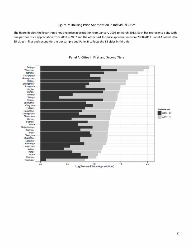
57
Figure 7: Housing Price Appreciation in Individual Cities
The figure depicts the logarithmic housing price appreciation from January 2003 to March 2013. Each bar represents a city with
one part for price appreciation from 2003 ‐‐ 2007 and the other part for price appreciation from 2008‐2013. Panel A collects the
35 cities in first and second tiers in our sample and Panel B collects the 85 cities in third tier.
Panel A: Cities in First and Second Tiers

58
Panel B: Cities in Third Tier

59
Figure 8: Comparing Housing Price Indices
This figure compares the monthly housing price indices for the four first‐tier cities constructed by us with the two
official series provided by the National Bureau of Statistics (NBS). In each of the panels, the solid line represents our
index, the dotted line presents the NBS average price index, and the dashed line the NBS 70‐city index.

60
Figure 9: Housing Price and GDP Growth in Japan and Singapore
Panel A depicts the Urban Land Price Index for Japan (average assessment value index) provided by the Japan Real Estate
Institute, together with the per capita GDP provided by the Japanese Statistics Bureau (Japan Statistical Yearbook), from 1955 to
2014. Panel B depicts the private property resale price index for Singapore (a median sale price index) provided by the Urban
Redevelopment Authority of Singapore, together with the per capita GDP of Singapore provided by the IMF, from 1975 to 2010.

61
Figure 10: Annual Income of Mortgage Borrowers
This figure depicts the time‐series of the household incomes of p10 and p50 for first‐, second‐, and third‐tier cities in
Panels A, B, and C, respectively. In panels A and B, the left plot shows the annual income of p10 and p50 (which is
averaged across all cities in the tier) from 2003‐2012, and the right plot shows the position of p10 and p50 in the
income distribution of the city population based on the income distribution reported by the Urban Household Survey
(UHS). Panel C shows only the annual income of p10 and p50.
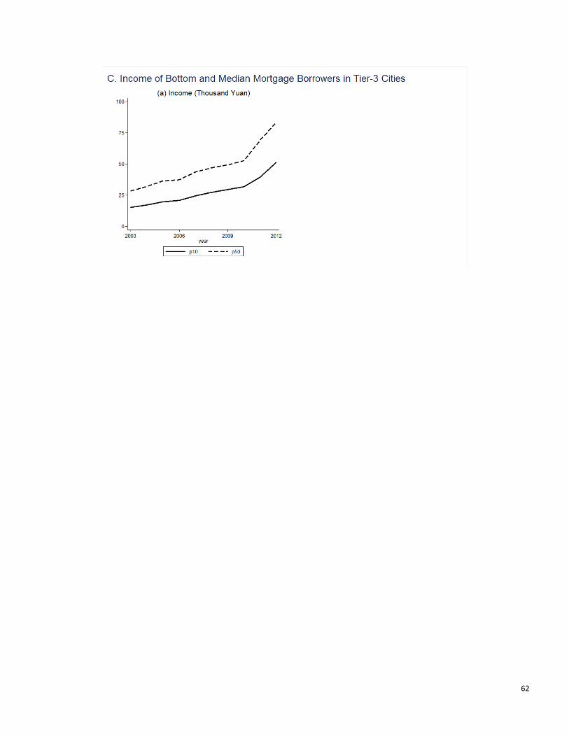
62
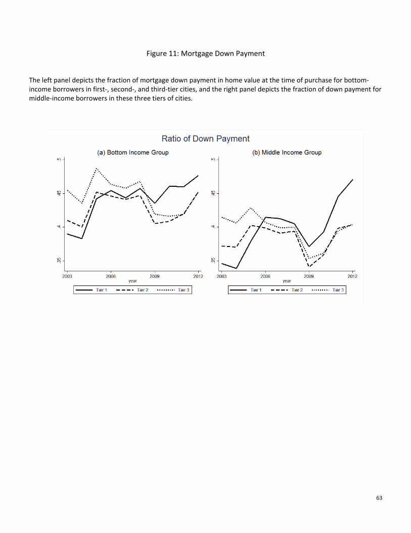
63
Figure 11: Mortgage Down Payment
The left panel depicts the fraction of mortgage down payment in home value at the time of purchase for bottom‐income borrowers in first‐, second‐, and third‐tier cities, and the right panel depicts the fraction of down payment for middle‐income borrowers in these three tiers of cities.

64
Figure 12: Price‐to‐Income Ratio of Mortgage Borrowers
This figure depicts the price‐to‐income ratio of mortgage borrowers in the full sample (top panel) and in the
subsample of married borrowers (bottom panel). In each panel, there are two plots, the left plot covers the
borrowers in the bottom‐income group with a separate line for each of the three tiers of cities, while the right plot
covers the borrowers in the middle‐income group.

65
Figure 13: Home Size of Mortgage Borrowers
The left panel depicts the home size of bottom‐income borrowers in first‐, second‐, and third‐tier cities, while the
right panel depicts that of middle‐income borrowers.

66
Figure 14: Age of Mortgage Borrowers
The left panel depicts the age of bottom‐income borrowers in first, second, and third tier cities, while the right panel
depicts that of middle‐income borrowers.

67
Figure 15: Marital Status of Mortgage Borrowers
The top panel depicts the fractions of single men and single women among middle‐income borrowers in three
separate plots for first, second, and third tier cities, while the bottom panel depicts these fractions among bottom‐
income borrowers in three separate plots for first, second, and third tier cities.
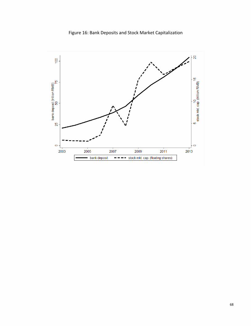
68
Figure 16: Bank Deposits and Stock Market Capitalization

69
Figure 17: Shanghai Stock Market Index

70
Figure 18: Share of Land Revenue in City Budget The top panel depicts the national average of share of land sales revenue in cities' fiscal budgets, while the bottom panel depicts the average among first‐tier cities, second‐tier cities and all other cities. Data Source: China Municipal Statistical Yearbook and China National Land Resource Yearbook.
0.1
.2.3
.4.5
.6.7
.8.9
1
2003 2005 2007 2009 2011
0.1
.2.3
.4.5
.6.7
.8.9
1
2003 2005 2007 2009 2011
Tier-1 Tier-2 Others

71
Table 1: Summary Statistics of Housing Return and Growth of GRP and Disposable Income, by Tier of Cities
Panel A: Nominal Growth
January 2003 ‐ December 2007 January 2009 ‐March 2013 January 2003 ‐March 2013
Nominal Growth Obs Mean Std. Dev. Min Max Mean Std. Dev. Min Max Mean Std. Dev. Min Max
Tier‐1 Cities
Housing Price Index 4 .210 .027 .172 .230 .177 .033 .139 .219 .159 .031 .128 .200
Per capita GRP index 4 .114 .020 .097 .144 .066 .020 .038 .081 .094 .016 .074 .112
Per capita DI index (urban) 4 .099 .025 .061 .116 .102 .003 .098 .105 .093 .028 .051 .110
Tier‐2 Cities
Housing Price Index 31 .168 .056 .021 .290 .116 .034 .043 .216 .132 .022 .082 .189
Per capita GRP index 30 .136 .050 .010 .235 .129 .031 .052 .191 .134 .033 .042 .189
Per capita DI index (urban) 30 .119 .025 .055 .178 .113 .013 .098 .164 .117 .015 .078 .152
Tier‐3 Cities
Housing Price Index 85 .113 .067 ‐.099 .250 .114 .036 .041 .242 .106 .036 .007 .178
Per capita GRP index 85 .154 .045 .006 .260 .140 .036 .037 .214 .150 .032 .030 .231
Per capita DI index (urban) 74 .118 .020 .059 .186 .117 .011 .087 .141 .117 .012 .079 .154
Panel B: Real Growth January 2003 ‐ December 2007 January 2009 ‐March 2013 January 2003 ‐March 2013
Real Growth Obs Mean Std. Dev. Min Max Mean Std. Dev. Min Max Mean Std. Dev. Min Max
Tier‐1 Cities
Housing Price Index 4 .187 .027 .148 .206 .151 .033 .113 .193 .131 .031 .100 .172
Per capita GRP index 4 .090 .020 .074 .120 .040 .020 .012 .055 .067 .016 .046 .085
Per capita DI index (urban) 4 .075 .025 .038 .092 .076 .003 .072 .079 .066 .028 .024 .083
Tier‐2 Cities
Housing Price Index 31 .145 .056 ‐.002 .266 .090 .034 .017 .190 .105 .022 .054 .162
Per capita GRP index 30 .113 .050 ‐.013 .212 .103 .031 .026 .165 .107 .033 .015 .161 Per capita DI index (urban) 30 .095 .025 .031 .154 .087 .013 .072 .138 .090 .015 .050 .125
Tier‐3 Cities
Housing Price Index 85 .090 .067 ‐.123 .227 .089 .036 .015 .216 .079 .036 ‐.021 .150
Per capita GRP index 85 .131 .045 ‐.018 .236 .114 .036 .011 .188 .123 .032 .003 .204 Per capita DI index (urban) 74 .094 .020 .036 .162 .091 .011 .061 .115 .089 .012 .052 .127

72
Table 2: Fraction of Second Mortgages
2011 2012 2013
First‐Tier Cities 5.3% 5.2% 11.8%Second‐Tier Cities 2.0% 2.4% 3.3%Third‐Tier Cities 1.0% 1.3% 1.8%
Table 3: Summary Statistics of Annual Returns of the Shanghai Stock Market Index (2003‐2013)
Mean Std. Dev. Skewness
2003‐2013 .073 .515 ‐.153 2003‐2008 .0898 .662 ‐.337 2009‐2013 .053 .339 1.182
Table 4: Summary Statistics of Annual Housing Returns (2003‐2013)
Full Sample (2003‐2013)
Mean Std. Dev. Skewness
First‐Tier Index .157 .154 ‐.674 Second‐Tier Index .135 .0989 .564 Third‐Tier Index .110 .075 .092
Before 2009 (2003‐2008)
Mean Std. Dev. Skewness
First‐Tier Index .204 .105 ‐.059 Second‐Tier Index .173 .099 .852 Third‐Tier Index .117 .095 ‐.028
After 2009 (2009‐2013)
Mean Std. Dev. Skewness
First‐Tier Index .109 .191 ‐.249 Second‐Tier Index .097 .094 .474 Third‐Tier Index .103 .059 ‐.057