Demographic Change, Human Capital and Welfare∗

Alexander Ludwig† Thomas Schelkle‡ Edgar Vogel§

June 3, 2011

Abstract

Projected demographic changes in the U.S. will reduce the share of the working-agepopulation. Analyses based on standard OLG models predict that these changes will in-crease the capital-labor ratio. Hence, rates of return to capital decrease and wages increase,which has adverse welfare consequences for current cohorts who will be retired when therate of return is low. This paper argues that adding endogenous human capital accumu-lation to the standard model dampens these forces. We find that this adjustment channelis quantitatively important. The standard model with exogenous human capital predictswelfare losses up to 12.5% (5.6%) of lifetime consumption, when contribution (replacement)rates to the pension system are kept constant. These numbers reduce to approximately8.7% (4.4%) when human capital can endogenously adjust.

JEL classification: C68, E17, E25, J11, J24Keywords: population aging; human capital; rate of return; distribution of welfare

∗We thank the editor, Gianluca Violante, and two anonymous referees for very valuable comments. We alsothank Alan Auerbach, Juan Carlos Conesa, Fatih Guvenen, Wouter Den Haan, Burkhard Heer, Berthold Her-rendorf, Andreas Irmen, Dirk Kruger, Wolfgang Kuhle, Michael Reiter, Richard Rogerson, Alice Schoonbroodt,Uwe Sunde, Matthias Weiss and several seminar participants at the ECB, IMF, LSE, University of Amsterdam,Universitat Bonn, Universitat Frankfurt, Universitat Konstanz, Universitat Mannheim, Universitat Wurzburg,the 13th International Conference of the Society for Computational Economics in Montreal, the 24th AnnualCongress of the European Economic Association in Barcelona and the Annual Meeting of the German EconomicAssociation (VfS) 2008 for helpful discussions. Financial support from the German National Research Founda-tion (DFG) through SFB 504, the State of Baden-Wurttemberg and the German Insurers Association (GDV) isgratefully acknowledged.

†CMR, Department of Economics and Social Sciences, University of Cologne; Albertus-Magnus-Platz; 50923Cologne; Email: ludwig@wiso.uni-koeln.de.

‡London School of Economics (LSE); Houghton Street; London WC2A 2AE; United Kingdom; Email:t.schelkle@lse.ac.uk.

§Mannheim Research Institute for the Economics of Aging (MEA); Universitat Mannheim; L13, 17; 68131Mannheim; Email: vogel.edgar@utanet.at.

1

1 Introduction

As in all major industrialized countries, the population of the United States is ag-

ing over time. This process is driven by increasing life expectancy and a decline

in birth rates from the peak levels of the baby boom. Consequently, the fraction

of the working-age population will decrease, and the fraction of elderly people will

increase. Figure 1 presents two summary measures of these demographic changes:

the working-age population ratio is predicted to decrease from 84% in 2005 to

75% in 2050, while the old-age dependency ratio will increase from 19% in 2005

to 34% in 2050. These projected changes in the population structure will have

important macroeconomic effects on the balance between physical capital and labor.

Specifically, labor is expected to be scarce relative to physical capital, with an en-

suing decline in real returns on physical capital and increases in gross wages. These

relative price changes have adverse welfare effects, especially for individuals close

to retirement because they receive a lower return on their assets accumulated for

retirement and cannot profit from increased wages.

This paper argues that a strong incentive to invest in human capital emanates

from the combined effects of increasing life expectancy and changes in relative prices,

particularly if social security systems are reformed such that contribution rates re-

main constant. At general equilibrium, such endogenous human-capital adjustments

substantially mitigate the effects of demographic change on macroeconomic aggre-

gates and individual welfare.

2

Figure 1: Working-Age and Old-Age Dependency Ratio

2005 2010 2015 2020 2025 2030 2035 2040 2045 205070

80

90

Year

WA

PR

[in

%]

Working−Age Population and Old−Age Dependency Ratio

2005 2010 2015 2020 2025 2030 2035 2040 2045 20500

20

40

OA

DR

[in

%]

WAPR [in %]OADR [in %]

Notes: Working-age population ratio (WAPR, left scale): ratio of population of age 16− 64 to total

adult population of age 16− 90. Old-age dependency ratio (OADR, right scale): ratio of population

of age 65− 90 to working-age population.

Source: Own calculations based on Human Mortality Database (2008).

The key contribution of our paper is to show that the human-capital adjustment

mechanism is quantitatively important. We add endogenous human-capital accumu-

lation to an otherwise standard large-scale OLG model in the spirit of Auerbach and

Kotlikoff (1987). The central focus of our analysis is then to work out the differences

between our model, with endogenous human capital adjustments and endogenous

labor supply, and the “standard” models in the literature, with fixed (exogenous)

productivity profiles.

We find that the decrease of the return to physical capital induced by demo-

graphic change in a model with endogenous human capital is only one-third of that

predicted in the standard model. Welfare consequences from increasing wages, de-

clines in rates of return, changes to pension contributions and benefits induced by

3

demographic change are substantial. When human capital cannot adjust, some of

the agents alive in 2005 will experience welfare losses up to 12.5% (5.6%) of life-

time consumption with constant pension contribution (replacement) rates. However,

importantly, we find that these maximum losses are only 8.7% (4.4%) of lifetime

consumption when the human capital adjustment mechanism is taken into account.

Ignoring this adjustment channel thus leads to quantitatively important biases of the

welfare assessment of demographic change.

Our work relates to a vast number of papers that have analyzed the economic

consequences of population aging and possible adjustment mechanisms. Important

examples in closed economies with a focus on social-security adjustments include

Huang et al. (1997), De Nardi et al. (1999) and, with respect to migration, Storeslet-

ten (2000). In open economies, Borsch-Supan et al. (2006), Attanasio et al. (2007)

and Kruger and Ludwig (2007), among others, investigate the role of international

capital flows during a demographic transition. We add to this literature by highlight-

ing an additional mechanism through which households can respond to demographic

change.

Our paper is closely related to the theoretical work on longevity, human capital,

taxation and growth1 and to Fougere and Merette (1999) and Sadahiro and Shima-

sawa (2002), who also quantitatively investigate demographic change in large-scale

OLG models with individual human-capital decisions. In contrast to their work,

1See, for example, de la Croix and Licandro (1999), Boucekkine et al. (2002), Kalemli-Ozcan et al. (2000)Echevarria and Iza (2006), Heijdra and Romp (2008), Ludwig and Vogel (2009) and Lee and Mason (2010). Ourpaper is also related to the literature emphasizing the role of endogenous human-capital accumulation for theanalysis of changes to the tax or social-security system, as in Lord (1989), Trostel (1993), Perroni (1995), Duporet al. (1996) and Lau and Poutvaara (2006), among others.

4

we focus our analysis on relative price changes during a demographic transition and

therefore consider an exogenous growth specification.2 We also extend their analysis

along various dimensions. We use realistic demographic projections instead of styl-

ized scenarios. More importantly, our model contains a labor supply-human capital

formation-leisure trade-off. It can thus capture effects from changes in individual

labor supply, i.e., human capital utilization, on the return of human-capital invest-

ments. As has already been stressed by Becker (1967) and Ben-Porath (1967), it is

important to model human-capital and labor supply-decisions jointly in a life-cycle

framework. Along this line, a key feature of our quantitative investigation is to em-

ploy a Ben-Porath (1967) human-capital model and calibrate it to replicate realistic

life-cycle wage profiles.3 Furthermore, we place particular emphasis on the welfare

consequences of an aging population for households living through the demographic

transition.

The paper is organized as follows. In Section 2, we present our quantitative

model. Section 3 describes the calibration strategy and our computational solution

method. Our results are presented in Section 4. Finally, Section 5 concludes the

paper. A separate online appendix4 contains additional results, robustness checks, a

description of our demographic model and technical details.

2Whether the trend growth rate endogenously fluctuates during the demographic transition or is held constantis of minor importance for the questions we are interested in. This is shown in our earlier unpublished workingpaper. The results are available upon request.

3The Ben-Porath (1967) model of human capital accumulation is one of the workhorses in labor economicsused to understand such issues as educational attainment, on-the-job training, and wage growth over the lifecycle, among others. See Browning, Hansen, and Heckman (1999) for a review. Extended versions of the modelhave been applied to study the significant changes to the U.S. wage distribution and inequality observed sincethe early 1970s by Heckman, Lochner, and Taber (1998) and Guvenen and Kuruscu (2009).

4The online appendix is available at www.wiso.uni-koeln.de/aspsamp/cmr/alexludwig/downloads/HKApp.pdf.

5

2 The Model

We employ a large-scale OLG model a la Auerbach and Kotlikoff (1987) with en-

dogenous labor supply and endogenous human-capital formation. The population

structure is exogenously determined by time- varying demographic processes for fer-

tility and mortality, the main driving forces of our model.5 In a perfectly competitive

environment, firms produce with standard constant returns to scale production func-

tion. We assume that the U.S. is a closed economy.6 Agents contribute a share of

their wages to the pension system, and retirees receive a share of their average in-

dexed past yearly earnings as pensions. Technological progress is exogenous.

2.1 Timing, Demographics and Notation

Time is discrete, and one period corresponds to one calendar year t. Each year, a

new generation is born. Birth in this paper refers to the first time households make

their own decisions and is set to the age of 16 (model age j = 0). Agents retire at

an exogenously given age of 65 (model age jr = 49). Agents live at most until age

90 (model age j = J = 74). At a given point in time t, individuals of age j survive

to age j + 1 with probability φt,j, where φt,J = 0. The number of agents of age j at

time t is denoted by Nt,j, and Nt =∑J

j=0Nt,j is the total population in t.

5We do not model endogenous life expectancy, fertility or endogenous migration and assume that all exogenousmigration is completed before agents begin making economically relevant decisions (cf. online Appendix C). Thus,we also abstract from potential feedback effects of social-security policies on fertility, as studied by Ehrlich andKim (2007).

6For our question, the assumption of a closed economy is a valid approximation. As documented in Krugerand Ludwig (2007), demographically induced changes in the return to physical capital and wages from the U.S.perspective do not differ much between closed- and open-economy scenarios. The reason is that demographicprocesses are correlated across countries and, in terms of speed of the aging processes, the U.S. is somewhere inthe middle with respect to all OECD countries.

6

2.2 Households

Each household comprises one representative agent who makes decisions regarding

consumption and saving, labor supply and human-capital investment. The household

maximizes lifetime utility at the beginning of economic life (j = 0) in period t,

maxJ∑j=0

βjπt,j1

1− σ{cϕt+j,j(1− ℓt+j,j − et+j,j)

1−ϕ}1−σ, σ > 0, ϕ ∈ (0, 1), (1)

where the per-period utility function is a function of individual consumption c, labor

supply ℓ and the time invested in formation of human capital, e. The agent is

endowed with one unit of time, thus, 1 − ℓ − e is leisure time. β is the pure time-

discount factor, ϕ determines the weight of consumption in utility, and σ is the

inverse of the inter-temporal elasticity of substitution with respect to the Cobb-

Douglas aggregate of consumption and leisure time. πt,j denotes the (unconditional)

probability to survive until age j, πt,j =∏j−1

i=0 φt+i,i, for j > 0 and πt,0 = 1.

Agents earn labor income (pension income when retired) as well as interest pay-

ments on their savings and receive accidental bequests. When working, they pay a

fraction τt from their gross wages to the social-security system. The net wage in-

come in period t of an agent of age j is given by wnt,j = ℓt,jht,jwt(1− τt), where wt is

the gross wage per unit of supplied human capital at time t. There are no annuity

markets, and households leave accidental bequests. These are collected by the gov-

ernment and redistributed in a lump-sum fashion to all households. Accordingly, the

7

dynamic budget constraint is given by

at+1,j+1 =

(at,j + trt)(1 + rt) + wnt,j − ct,j if j < jr

(at,j + trt)(1 + rt) + pt,j − ct,j if j ≥ jr,

(2)

where at,j denotes assets, trt are transfers from accidental bequests, rt is the real

interest rate, the rate of return to physical capital, and pt,j is pension income. Initial

household assets are zero (at,0 = 0), and the transversality condition is at,J+1 = 0.

2.3 Formation of Human Capital

The key element of our model is the endogenous formation of human capital. House-

holds enter economic life with a predetermined and cohort invariant level of human

capital ht,0 = h0. Afterwards, they can invest a fraction of their time into acquiring

additional human capital. We adopt a version of the Ben-Porath (1967) human-

capital technology7 given by

ht+1,j+1 = ht,j(1− δh) + ξ(ht,jet,j)ψ ψ ∈ (0, 1), ξ > 0, δh ≥ 0, (3)

where ξ is a scaling factor, the average learning ability, ψ determines the curvature

of human-capital technology, δh is the depreciation rate of human capital, and et,j is

time invested in human-capital formation.

The costs of investing in human capital in this model are only the opportunity

costs of foregone wage income and leisure. We understand the process of accumulat-

ing human capital to be a mixture of knowledge acquired by formal schooling and

7This functional form is widely used in the human-capital literature, cf. Browning, Hansen, and Heckman(1999) for a review.

8

on-the- job training programs after schooling is complete. Human capital can be

accumulated until retirement age, but an agent’s optimally chosen time investment

converges to zero some time before retirement.

2.4 The Pension System

The pension system is a simple balanced-budget, pay-as-you-go system that resem-

bles key features of the U.S. system. Workers contribute a fraction τt of their gross

wages, and pensioners receive a fraction ρt of their average indexed past yearly earn-

ings.8 The level of pensions in each period is given by pt,j = ρtwt+jr−jht+jr−jst,jjr−1

,

where wt+jr−jht+jr−jst,jjr−1

are average indexed past yearly earnings (AIYE)9, wt+jr−jht+jr−j

are average earnings of all workers in the period when a retiree of current age j reaches

retirement age jr, and ht is defined as ht =∑jr−1

j=0 ℓt,jht,jNt,j∑jr−1j=0 Nt,j

. We refer to ht as the av-

erage (hours weighted) human-capital stock. The sum up to age j of past individual

earnings of an agent relative to average economy-wide earnings in the respective year

is given by st,j =∑j

i=0ℓt−j+i,iht−j+i,i

ht−j+i. This links pensions to individuals’ past earn-

ings. Using the above formula for pt,j, the budget constraint of the pension system

is given by

τtwt

jr−1∑j=1

ℓt,jht,jNt,j = ρt

J∑j=jr

Nt,jwt+jr−jht+jr−jst,j

jr − 1∀t. (4)

8The U.S. system applies an additional bend-point formula to pensions, which results in intra-generationalredistribution. However, in our model, without intra-cohort heterogeneity, we do not take this feature of theactual system into account. For a description of the current U.S. system, see Diamond and Gruber (1999) andGeanakoplos and Zeldes (2009).

9Our concept of AIYE is an approximation to the “average indexed monthly earnings” (AIME) in the currentU.S. system where only the 35 years of working life with the highest individual earnings relative to averageearnings are counted for the calculation of AIME. We ignore this feature for computational reasons and countall years of working life.

9

Below, we consider two opposite scenarios of parametric adjustment of the pension

system to demographic change. In our first scenario (“const. τ”), we hold the

contribution rate constant, τt = τ , and endogenously adjust the replacement rate to

balance the budget of the pension system. In the other extreme scenario (“const.

ρ”), we hold the replacement rate constant, ρt = ρ, and endogenously adjust the

contribution rate.

2.5 Firms and Equilibrium

Firms operate in a perfectly competitive environment and produce one homogenous

good, according to the Cobb-Douglas production function

Yt = Kαt (AtLt)

1−α, (5)

where α denotes the share of capital used in production. Kt, Lt and At are the stocks

of physical capital, effective labor and the level of technology, respectively. Output

can be either consumed or used as an investment good. We assume that labor inputs

and human capital of different agents are perfect substitutes, and effective labor

input Lt is accordingly given by Lt =∑jr−1

j=0 ℓt,jht,jNt,j. Factors of production are

paid their marginal products, i.e., wt = (1 − α) YtLt

and rt = α YtKt

− δt, where wt is

the gross wage per unit of efficient labor, rt is the interest rate, and δt denotes the

depreciation rate of physical capital. Total factor productivity, At, is growing at the

exogenous rate of gAt : At+1 = At(1 + gAt ).

The definition of equilibrium is standard and can be found in our online Appendix

A.

10

2.6 Thought Experiments

We take as an exogenous driving process a time-varying demographic structure.

Computations begin in year 1750 (t = 0), assuming an artificial initial steady state10.

We then compute the model equilibrium from 1750 to 2500 (t = T = 751) when

the new steady state is assumed and reached11 and report simulation results for the

main projection period of interest, from 2005 (t = 256) to 2050 (t = 306). We use

data during our calibration period, 1960 − 2005 (from t0 = 211 to t1 = 256), to

determine several structural model parameters (cf. section 3).

Our main objective is to compare the time paths of aggregate variables and welfare

across two model variants for two social-security scenarios. Our first model variant

is one in which households adjust their human capital, and our second variant is one

in which human capital is held constant across cohorts. Therefore, our strategy is

to first solve for transitional dynamics using the model described above. Next, we

use the endogenously obtained profile of time invested in human-capital formation

to compute an average time investment and associated human-capital profile, which

is then fed into our alternative model in which agents are restricted with respect to

their time-investment choice. We do so separately for the two opposite social-security

scenarios described in subsection 2.4. The average time investment is computed as

ej = 1t1−t0+1

∑t1t=t0

et,j for our calibration period (t0 = 211 and t1 = 256). In the

10The artificial initial steady state and long phase-in period are only used to generate suitable starting valuesfor our main projection period. Bar and Leukhina (2010) provide an explicit model of the demographic transitionand economic development that began in 17th Century England.

11In fact, changes in variables that are constant in steady state are already numerically irrelevant circa theyear 2400.

11

alternative model, we then add the constraint et,j = ej. The human-capital profile

is then obtained from (3) by iterating forward on age.12

3 Calibration and Computation

To calibrate the model, we choose model parameters such that simulated moments

match selected moments in NIPA data and the endogenous wage profiles match the

empirically observed wage profile in the U.S. during the calibration period 1960 −

2005.13 The calibrated parameters are summarized in Table 1.

Table 1: Model Parameters

Preferences σ Inverse of Inter-Temporal Elasticity of Substitution 2.00β Pure Time Discount Factor 0.993ϕ Weight of Consumption 0.401

Human Capital ξ Scaling Factor 0.16ψ Curvature Parameter 0.65δh Depreciation Rate of Human Capital 0.8%h0 Initial Human Capital Endowment 1.00

Production α Share of Physical Capital in Production 0.33δ Depreciation Rate of Physical Capital 3.8%gA Exogenous Growth Rate 1.8%

12By imposing the restriction of identical time-investment profiles for all cohorts (instead of, e.g., imposingthe restriction only on cohorts born after 2005), we shut down direct effects from changing mortality on humancapital and indirect anticipation effects of changing returns. This alternative model is a “standard” model ofendogenous labor supply and an exogenously given age-specific productivity profile—as used in numerous studieson the consequences of demographic change—with the only exception being that the time endowment is age-specific. By setting the time endowment to 1 − ej rather than 1, we avoid re-calibration across model variants.For details, see below.

13We perform this moment matching in the endogenous human-capital model and the constant contribution-rate scenario. We do not recalibrate model parameters across social-security scenarios or for the alternativehuman-capital model because simulated moments do not differ much. Furthermore, we are interested in howour welfare conclusions are affected by imposing various constraints on the model—either through our social-security scenarios or by restricting human-capital formation—and any parametric change in this comparisonwould confound our welfare analysis.

12

3.1 Demographics

Actual population data from 1950− 2005 are collected from the Human Mortality

Database (2008). Our demographic projections beyond 2004 are based on a popu-

lation model that is described in detail in the online Appendix C.14 Prior to 1950,

we keep the population structure constant, as in 1950.

3.2 Household Behavior

The parameter σ, the inverse of the inter-temporal elasticity of substitution, is set

to 2.15 The time-discount factor β is calibrated to match the empirically observed

capital-output ratio of 2.8 which requires β = 0.993. The weight of consumption

in the utility function, ϕ, is calibrated such that households spend one-third of their

time working, on average, which requires ϕ = 0.401.

3.3 Individual Productivity Profiles

We choose values for the parameters of the human-capital production function such

that average simulated wage profiles resulting from endogenous human-capital forma-

tion replicate empirically observed wage profiles. Data for age-specific productivity

are collected from Huggett et al. (2010)16. We first normalize h0 = 1 and then deter-

14The key assumptions of this model are as follows: First, the total fertility rate is constant at 2005 levels of2.0185, until 2100, when fertility is adjusted slightly to keep the number of newborns constant for the remainderof the simulation period. Second, life expectancy monotonically increases from a current (2004) average lifeexpectancy at birth of 77.06 years to 88.42 years in 2100, when it is held constant. Third, total migration isconstant at the average migration for 1950−2005 for the remainder of the simulation period. These assumptionsimply that a stationary population is reached in about 2200.

15In the online appendix, Section B.4, a sensitivity analysis shows that our main quantitative results are robustwhen we change the predetermined parameter σ to 1 or 3, respectively.

16We thank Mark Huggett for sending us the data.

13

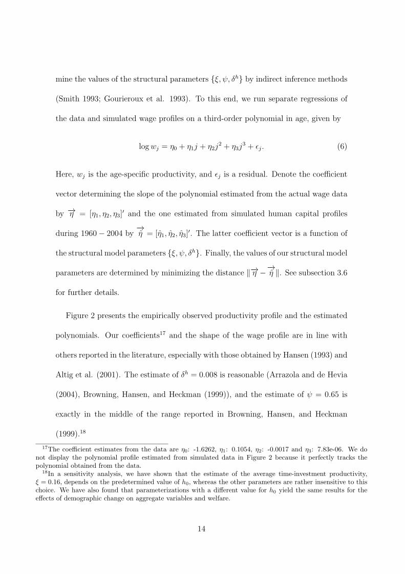
mine the values of the structural parameters {ξ, ψ, δh} by indirect inference methods

(Smith 1993; Gourieroux et al. 1993). To this end, we run separate regressions of

the data and simulated wage profiles on a third-order polynomial in age, given by

logwj = η0 + η1j + η2j2 + η3j

3 + ϵj. (6)

Here, wj is the age-specific productivity, and ϵj is a residual. Denote the coefficient

vector determining the slope of the polynomial estimated from the actual wage data

by −→η = [η1, η2, η3]′ and the one estimated from simulated human capital profiles

during 1960− 2004 by−→η = [η1, η2, η3]

′. The latter coefficient vector is a function of

the structural model parameters {ξ, ψ, δh}. Finally, the values of our structural model

parameters are determined by minimizing the distance ∥−→η −−→η ∥. See subsection 3.6

for further details.

Figure 2 presents the empirically observed productivity profile and the estimated

polynomials. Our coefficients17 and the shape of the wage profile are in line with

others reported in the literature, especially with those obtained by Hansen (1993) and

Altig et al. (2001). The estimate of δh = 0.008 is reasonable (Arrazola and de Hevia

(2004), Browning, Hansen, and Heckman (1999)), and the estimate of ψ = 0.65 is

exactly in the middle of the range reported in Browning, Hansen, and Heckman

(1999).18

17The coefficient estimates from the data are η0: -1.6262, η1: 0.1054, η2: -0.0017 and η3: 7.83e-06. We donot display the polynomial profile estimated from simulated data in Figure 2 because it perfectly tracks thepolynomial obtained from the data.

18In a sensitivity analysis, we have shown that the estimate of the average time-investment productivity,ξ = 0.16, depends on the predetermined value of h0, whereas the other parameters are rather insensitive to thischoice. We have also found that parameterizations with a different value for h0 yield the same results for theeffects of demographic change on aggregate variables and welfare.

14

Figure 2: Wage Profiles

25 30 35 40 45 50 55 600.6

0.7

0.8

0.9

1

1.1

Age

Wag

e

Wage Profile

Observed ProfilePolynomials

Notes: Observed profile: average life-cycle wage profiles collected from Huggett, Ventura, and Yaron(2010). Polynomials: predicted wage profile based on estimated polynomial coefficients of (6). Bothprofiles were normalized by their respective means.

3.4 Production

We calibrate the capital share in production, α, to match the income share of labor

in the data, which requires that α = 0.33. We estimate a series of TFP and actual

depreciation using NIPA data. We HP-filter these data series and then feed them

into the model for the period 1950 to 2005. Thereafter, both parameters, g and

δ, are held constant at their respective means. The average growth rate of total

factor productivity, gA, is calibrated to match the growth rate of the Solow residual

in the data. Accordingly, gA = 0.018. Finally, we calibrate δ (and thereby scale

the exogenous time path of depreciation, δt) such that our simulated data match an

average investment-output ratio of 20%, which requires δ = 0.038.

15

3.5 The Pension System

In our first social-security scenario (“const. τ”), we fix contribution rates and adjust

replacement rates of the pension system. We calculate contribution rates from NIPA

data for 1960 − 2004 and freeze the contribution rate at the year-2004 level for

all following years. When simulating the alternative social-security scenario with

constant replacement rates (“const. ρ”), we feed the equilibrium replacement rate

obtained in the “const. τ” scenario into the model and hold it constant at the 2004

level for all remaining years. Then the contribution rate endogenously adjusts to

balance the budget of the social-security system.

3.6 Computational Method

For a given set of structural model parameters, the solution of the model is deter-

mined by outer- and inner-loop iterations. On the aggregate level (outer loop), the

model is solved by guessing initial time paths of four variables: the capital intensity,

the ratio of bequests to wages, the replacement rate (or contribution rate) of the

pension system and average human capital for all periods from t = 0 until T . On the

individual level (inner loop), we begin each iteration by guessing the terminal values

for consumption and human capital. We then proceed by backward induction and

iterate over these terminal values until the inner-loop iterations converge. In each

outer loop, disaggregated variables are aggregated each period. We then update ag-

gregate variables until convergence, using the Gauss-Seidel-Quasi-Newton algorithm

developed in Ludwig (2007).

16

To calibrate the model in the “const. τ” scenario, we consider additional “outer

outer” loops to determine structural model parameters by minimizing the distance

between the simulated average values and their respective calibration targets for the

calibration period 1960− 2004. To summarize the description above, the parameter

values determined in this way are β, ϕ, δ, ξ, ψ and δh.

4 Results

Before using our model to investigate the effects of future demographic change, we

show how well it can replicate observed individual life-cycle profiles of the past.

Next, we turn to the analysis of the transitional dynamics for the period 2005 to

2050, whereby we focus especially on the developments of major macroeconomic

variables and the welfare effects of demographic change.

4.1 Backfitting

We first examine consumption profiles. We recognize that our model fails to replicate

the empirically observed cross-sectional consumption profile in the 1990 Consumer

Expenditure Survey19, cf. Figure 3(a). The increase of consumption over the life

cycle is too steep, and the peak is too late compared to the data. Because the

decrease of consumption after the peak is solely caused by falling survival rates in a

model without idiosyncratic risk, we cannot expect to match this dimension of the

19The empirical profile is based on the observations on non-durable consumption for 1990 in the data set ofAguiar and Hurst (2009). We equalize the data using the traditional OECD scale that attributes weights of(1.0, 0.7, 0.5) to the first adult, further adults (above age 16) and children, respectively. We then estimate athird-order polynomial in age on the adult-equivalent consumption data and show the predicted profile in thefigure.

17

data (cf. Hansen and Imrohoroglu (2008), Fernandez-Villaverde and Kruger (2007)).

As shown in Ludwig et al. (2007), in a model without human-capital adjustments,

omitting idiosyncratic risk has only a negligible effect on welfare calculations. This

is because welfare calculations are based on differences in consumption profiles, and

the exact shape of the consumption profile is therefore less important. However,

verifying the robustness of this finding in a model with endogenous human capital

such as ours requires the introduction of idiosyncratic risk. We leave this extension

for future research, mainly for technical reasons.20

We next examine asset profiles. Figure 3(b) shows household net worth data from

the Survey of Consumer Finances for a cross-section in 1995, obtained from Bucks

et al. (2006), and the corresponding cross-sectional asset profile in the model. Our

model matches the broad pattern in the data. Observed discrepancies are threefold:

First, as borrowing constraints are absent from our model, initial assets are negative,

whereas they are positive in the data. Second, the run-up of wealth until retirement

age is stronger in our model than it is in the data. Third, decumulation of assets is

stronger as well. This last fact is due to the fact that our model neither has health

risks, as in De Nardi et al. (2009), nor explicit bequest motives, cf., e.g., Attanasio

(1999).

20Introducing idiosyncratic risk into our large model with two continuous-state variables would render compu-tation of the transition path practically infeasible. However, to address the sensitivity of our welfare results withrespect to the consumption profile, we have performed an additional sensitivity check, whereby we introducelump-sum transfers that redistribute resources from aged individuals to young individuals within a household,such that the present value of lifetime resources is unaffected. This increases savings at younger ages. Ourcalibration then offsets this increase in savings via a lower β. This yields a flatter consumption profile. The totaleffect of lump-sum transfers on the consumption profile, therefore, mimics the effects of precautionary savings.This sensitivity analysis shows that our findings continue to hold in a model that achieves a better fit of theconsumption profile and is otherwise as close as possible to our benchmark model. The results are available uponrequest.

18

Figure 3: Cross-Sectional Profiles

(a) Consumption

20 30 40 50 60 70 800.5

0.6

0.7

0.8

0.9

1

1.1

1.2

1.3

1.4

1.5

Age

Co

nsu

mp

tio

n

Consumption in 1990

modeldata

(b) Assets

10 20 30 40 50 60 70 80 90−0.5

0

0.5

1

1.5

2

2.5

Age

Net

Wor

th

Net Worth in 1995

modeldata

(c) Labor Supply

20 25 30 35 40 45 50 55 600

0.05

0.1

0.15

0.2

0.25

0.3

0.35

0.4

0.45

0.5

Age

Ho

urs

Wo

rked

Hours Worked in 1990

modeldata

(d) Wages

20 25 30 35 40 45 50 55 600.5

0.6

0.7

0.8

0.9

1

1.1

1.2

1.3

Age

Wag

e

Wage Profile in 1990

modeldata

Notes: Model and data profiles for consumption, assets, labor supply and wages. All profiles are

cross-sectional profiles for 1990, except for the asset profile, which is for 1995. Consumption, asset

and wage profiles are normalized by their respective means. Hours data are normalized by 76 total

hours per week.

Data Sources: Based on CEX consumption data collected from Aguiar and Hurst (2009), SCF net

worth data obtained from Bucks et al. (2006), hours worked data from McGrattan and Rogerson

(2004) and PSID wage data.

Our model does a good job of matching the cross-sectional hours profile observed

in 1990 Census data collected from McGrattan and Rogerson (2004); see figure 3(c).21

21The hours data are normalized, with total hours per week equal to 76. This might appear to be a low numberfor total available hours, but such a magnitude is needed to make the McGrattan and Rogerson (2004) hours

19

Given our preference specification, the inverse u-shape of hours worked translates into

a u-shaped pattern of Frisch labor-supply elasticities over the life-cycle. This implic-

itly captures higher elasticities at the extensive margin at the beginning and end of

the life-cycle, cf., e.g., Rogerson and Wallenius (2009). Using a Frisch elasticity con-

cept with constant (variable) time invested in human-capital formation, we find that

agents of age 30-50 have an average elasticity of 0.8 (1.3). A more detailed discussion

of these concepts can be found in our online Appendix B.2. The hour-weighted aver-

age Frisch elasticity across all ages, a “macro” elasticity, is approximately 1.1 (1.9).

These numbers are higher than the standard microeconomic estimates reported in

the literature, which are typically approximately 0.5. See, e.g., Domeij and Floden

(2006). However, these standard estimates are based on prime-age, full-time em-

ployed, male workers. In contrast, Browning, Hansen, and Heckman (1999) report

that the scarce empirical estimates for females are much higher than for males. Our

model is a unisex model and should, accordingly, represent both sexes. Further-

more, Imai and Keane (2004) argue that standard estimates are downward-biased

by not considering endogenous human- capital accumulation explicitly and thereby

not correctly accounting for the true opportunity cost of time.22 We therefore regard

our value of the Frisch elasticity as very reasonable. In Section B.4 of the online

data broadly consistent with the common belief that agents spend about one-third of their time working andthe standard practice of macroeconomists to calibrate their models (which we have followed). The McGrattanand Rogerson (2004) data only contain average hours for certain age bins, e.g., average hours for persons of age15-24. We associate the average hours with the age mean of that age bin, e.g., associate the value for ages 15-24with age 20 and then use cubic interpolation to construct the empirical hours profile for all other ages. A similarprocedure is used to construct the empirical asset profile.

22Imai and Keane (2004) make this argument in the context of a learning-by-doing model, but similar biasesmight be present in our model. We are unaware of any attempt to estimate the Frisch elasticity with varyingtime invested empirically in a framework such as ours, which would require inclusion of the marginal utility ofhuman capital in the set of conditioning variables.

20

appendix, a sensitivity analysis further shows that our main quantitative results are

robust to using a higher value of σ, which implies a lower Frisch elasticity.

Finally, Figure 3(d) shows the cross-sectional wage profile observed in the PSID

data in 1990. Our model matches the broad pattern observed in the data.23

4.2 Transitional Dynamics

We divide our analysis of transitional dynamics into two parts. First, we analyze

the behavior of several important aggregate variables from 2005 to 2050. Second, we

investigate the welfare consequences of demographic change for generations already

alive in 2005 and for households born in the future. Throughout, we demonstrate

how the design of the social-security system affects our results.

4.2.1 Aggregate Variables

The evolution of policy variables in the two social-security scenarios is presented

in Figure 4. In the “const. τ” scenario, pensions become less generous over time,

which is represented by a decrease in the replacement rate, from approximately 73%

(74%) in 2005 to 41% (42%) in 2050 for the endogenous (exogenous) human-capital

model. In contrast, in the “const. ρ” scenario, the generosity of the pension system

remains at the 2005 level, implying that contribution rates have to increase from

approximately 12% in 2005 to 21% in 2050 in both human-capital models.24

23The wage data were selected using the same criteria as in Huggett, Ventura, and Yaron (2010). To smooththe data, we show a centered average of five subsequent PSID samples. In Section B.1 of the online appendix, wepresent the fit of our model to cross-sectional data on wages and hours in the years 1970, 1980, 1990 and 2000.The model profiles are broadly consistent with the data at all those points in time.

24As explained in Section 2.4, our model of the pension system abstracts from the fact that in the United States,only the 35 years of working life with the highest individual earnings relative to average earnings are counted for

21

Figure 4: Evolution of Policy Variables

(a) Contribution Rate

2005 2010 2015 2020 2025 2030 2035 2040 2045 205010

12

14

16

18

20

22

24

Year

Co

ntr

ibu

tio

n R

ate

in %

Contribution Rate

const. τ, endog. h.c.const. τ, exog. h.c.const. ρ, endog. h.c.const. ρ, exog. h.c.

(b) Replacement Rate

2005 2010 2015 2020 2025 2030 2035 2040 2045 205035

40

45

50

55

60

65

70

75

Year

Rep

lace

men

t R

ate

in %

Replacement Rate

const. τ, endog. h.c.const. τ, exog. h.c.const. ρ, endog. h.c.const. ρ, exog. h.c.

Notes: Pension system contribution and replacement rates for the two social-security scenarios.

“const. τ”: constant contribution-rate scenario. “const. ρ”: constant replacement-rate scenario.

“endog. h.c.”: endogenous human-capital model. “exog. h.c.”: exogenous human-capital model.

Figure 5 reports the dynamics of four major macroeconomic variables for the two

model variants—with endogenous and exogenous human capital—in the “const. τ”

social-security scenario, and Figure 6 does so in the “const. ρ” scenario.

In Figures 5(a) and 6(a), we show the evolution of the rate of return to physical

capital for the different models.25 In the “standard” models with endogenous labor

supply only, the rate of return decreases from an initial level of approximately 8.1%

in 2005 to 7.1% in the “const. τ” scenario and to 7.7% in the “const. ρ” scenario in

2050.26 This magnitude is in line with results reported elsewhere in the literature, cf.,

the calculation of average indexed past earnings. This leads us to overstate the replacement rate but does notdirectly affect the level of pensions. Furthermore, we assume a balanced budget, whereas the U.S. system runsa social-security trust fund that collects excess paid-in contributions. This biases upward the replacement rateand the level of pensions.

25There are two reasons for the small level differences in 2005 across the various scenarios. First, our calibrationtargets are averages for the period 1960− 2004. Second, as already discussed in Section 3, we do not recalibrateacross scenarios. Such level differences in initial values can be observed in all of the following figures.

26The high initial level of the rate of return is caused by the previous baby boom, which increased the labor

22

e.g., Borsch-Supan et al. (2006) and Kruger and Ludwig (2007), whereas Attanasio

et al. (2007) find slightly larger effects. On the contrary, in the two models with

endogenous human-capital adjustment, the rate of return is expected to fall by only

0.4 (0.2) percentage points in the “const. τ” (“const. ρ”) scenario. This difference in

the decrease of the rate of return until 2050 between the exogenous and endogenous

human-capital models is large, at a factor of about 2.5.

In Figures 5(b) and 6(b), we depict the evolution of average hours worked by all

working-age individuals. Average hours worked increase both for the endogenous and

exogenous human-capital models. Observe that there are level differences between

the two model variants. This is mainly caused by differences in time invested in

human-capital formation.

Figures 5(c) and 6(c) show that time invested in human-capital formation in-

creases when agents are allowed to adjust their human capital. The reasons for this

adjustment are that both higher wage growth and a lower rate of return to physi-

cal capital strengthen the incentive to accumulate human capital. Specifically, with

endogenous human capital in the “const. τ” (“const. ρ”) scenario, average human

capital per working hour increases by approximately 17% (11%) until 2050.

Finally, we focus on the evolution of the growth rate of GDP per capita, as shown

in Figures 5(d) and 6(d). When the U.S. aging process peaks in 2025 (cf. figure 1),

the growth rate of per-capita GDP falls in all scenarios to its lowest level. The drop is

least pronounced for the endogenous human capital model with a fixed contribution

force and hence decreased capital intensity.

23

Figure 5: Aggregate Variables for Constant Contribution-Rate Scenario

(a) Rate of Return to Physical Capital

2005 2010 2015 2020 2025 2030 2035 2040 2045 20506.5

7

7.5

8

8.5

Year

r in

%

Rate of Return

endog. h.c.exog. h.c.

(b) Average Hours Worked

2005 2010 2015 2020 2025 2030 2035 2040 2045 20500.33

0.335

0.34

0.345

0.35

0.355

0.36

0.365

0.37

Year

Ave

rag

e H

ou

rs W

ork

ed

Average Hours Worked

endog. h.c.exog. h.c.

(c) Average Human Capital

2005 2010 2015 2020 2025 2030 2035 2040 2045 20502.1

2.2

2.3

2.4

2.5

2.6

2.7

Year

Ave

rag

e H

um

an C

apit

al

Average Human Capital

endog. h.c.exog. h.c.

(d) Growth of GDP per Capita in %

2005 2010 2015 2020 2025 2030 2035 2040 2045 20501

1.5

2

2.5

Year

Gro

wth

of

GD

P p

er C

apit

a

Growth of GDP per Capita

endog. h.c.exog. h.c.

Notes: Rate of return to physical capital, average hours worked of the working-age population, average

human capital per working hour and growth of GDP per capita in the constant contribution-rate

social-security scenario for two model variants. “endog. h.c.”: endogenous human-capital model.

“exog. h.c.”: exogenous human capital model.

rate. There, the growth rate gradually declines from 2.2% in 2005 to 1.9% in 2025.27

Comparing the two “const. τ” scenarios, it can be observed that not adjusting

the human-capital profile entails a large drop in the growth rate. The maximum

difference circa 2025 is 0.4 percentage points. Although the difference across human-

27The high initial growth rate is a consequence of the past baby boom, cf. footnote 26.

24

Figure 6: Aggregate Variables for Constant Replacement-Rate Scenario

(a) Rate of Return to Physical Capital

2005 2010 2015 2020 2025 2030 2035 2040 2045 20506.5

7

7.5

8

8.5

Year

r in

%

Rate of Return

endog. h.c.exog. h.c.

(b) Average Hours Worked

2005 2010 2015 2020 2025 2030 2035 2040 2045 20500.33

0.335

0.34

0.345

0.35

0.355

0.36

0.365

0.37

Year

Ave

rag

e H

ou

rs W

ork

ed

Average Hours Worked

endog. h.c.exog. h.c.

(c) Average Human Capital

2005 2010 2015 2020 2025 2030 2035 2040 2045 20502.1

2.2

2.3

2.4

2.5

2.6

2.7

Year

Ave

rag

e H

um

an C

apit

al

Average Human Capital

endog. h.c.exog. h.c.

(d) Growth of GDP per Capita in %

2005 2010 2015 2020 2025 2030 2035 2040 2045 20501

1.5

2

2.5

Year

Gro

wth

of

GD

P p

er C

apit

a

Growth of GDP per Capita

endog. h.c.exog. h.c.

Notes: Rate of return to physical capital, average hours worked of the working-age population, average

human capital per working hour and growth of GDP per capita in the constant replacement-rate social-

security scenario for two model variants. “endog. h.c.”: endogenous human-capital model. “exog.

h.c.”: exogenous human-capital model.

capital models is only 0.2 percentage points in the case that the replacement rate

is held constant (“const. ρ” scenarios), the same conclusion applies. The aging

process induces relative price changes, such that agents increase their time invested

in human-capital formation and thereby cushion the negative effects of demographic

25

change on growth.28

4.2.2 Welfare Effects

In our model, a household’s welfare is affected by two consequences of demographic

change. First, her lifetime utility changes because her own survival probabilities

increase. Second, households face a path of declining interest rates, increasing gross

wages and decreasing replacement rates (increasing contribution rates) relative to

the situation without a demographic transition.

We want to isolate the welfare consequences of the second effect. To this end, we

compare for an agent born at time t and of current age j her lifetime utility when

she faces equilibrium factor prices, transfers and contribution (replacement) rates,

as documented in the previous section, with her lifetime utility when she instead

faces prices, transfers and contribution (replacement) rates that are held constant

at their 2005 value. For both of these scenarios, we fix the households’ individual

survival probabilities at their 2005 values.29 Following Attanasio et al. (2007) and

Kruger and Ludwig (2007), we then compute the consumption-equivalent variation

gt,j, i.e., the percentage increase in consumption that needs to be given to an agent

with characteristics t, j at each date in her remaining lifetime at fixed prices to

make her as well off as she would be in the situation with changing prices.30 Positive

28In our online Appendix B.3.1, we show that the cumulative effect of the growth rate differences between theendogenous and exogenous human-capital models on the level of GDP per capita is large. With human-capitaladjustments, the detrended level of GDP per capita will increase by approximately 14% (10%) more until 2050in the “const. τ” (“const. ρ”) scenario than without these adjustments.

29Of course, they fully retain their age dependency. We show in the online Appendix B.3.2 that varying thesurvival probabilities according to the underlying demographic projections leaves our conclusions on welfare inthe comparison across the two models essentially unchanged.

30With our assumptions on preferences, gt,j can be calculated as gt,j =(

Vt,j

V 2005j

) 1ϕ(1−σ) − 1, where Vt,j denotes

26

numbers of gt,j thus indicate that households obtain welfare gains from the general-

equilibrium effects of demographic change, and negative numbers indicate welfare

losses.

Welfare of Generations Alive in 2005

Of particular interest is how the welfare of all generations already alive in 2005 will

be affected by demographic change. This analysis allows for an inter-generational

welfare comparison of the consequences of demographic change in terms of well-

being that would not be possible using aggregate statistics such as per-capita GDP.

Newborns and young generations benefit from increasing wages as well as decreasing

returns, if they borrow to finance their human-capital formation. However, older—

and thus asset-rich—generations are expected to lose lifetime utility. First, they

benefit less from increasing wages because they do not significantly adjust their

human capital and because their remaining working period is short. Second, falling

returns diminish their capital income. Third, retirement income decreases in our

scenario with constant contribution rates.

The results shown in Figure 7 can be summarized as follows: First, the welfare of

newborn agents is essentially unchanged in the “const. τ” scenarios, whereas in the

“const. ρ” scenario, newborns experience welfare losses of roughly 4.4% (5.0%) in the

endogenous (exogenous) human-capital model. As explained in our online Appendix

B.3.2, the fact that these welfare changes are almost identical in the two human-

capital models is due to a complex interaction between the value of human-capital

lifetime utility at changing prices and V 2005j at fixed 2005 prices.

27

adjustments, which is positive, and differential general-equilibrium effects, which

partially offset this interaction. Second, middle-aged agents incur the highest losses

in the “const. τ” scenarios: the maximum loss of agents is much larger compared to

a scenario with fixed replacement rates. Clearly, constant replacement rates decrease

net wages of the young but keep pensions more generous. This decreases lifetime

utility of the young but narrows the loss of utility of the old (compared to a situation

with falling replacement rates). The redistribution through the pension system shifts

the balance somewhat in favor of the old. This also explains why the maximum of the

losses occurs at a much higher age in the “const. τ” scenario in which agents close

to retirement lose interest income and receive lower pensions. Third, independent

of future pension policy, agents lose relatively less in the endogenous human-capital

model. Younger agents can adjust their human capital in response to higher wages,

whereas older (asset-rich) households benefit from a smaller drop in the interest rate

(cf. Figures 5(a) and 6(a)) and higher pension payments.31

Table 2 finally provides numbers on the maximum welfare loss displayed in Figure

7 as a summary statistic. In the exogenous human-capital model, the maximum

welfare loss is approximately 12.5% (5.6%) of lifetime consumption in the “const.

τ” (“const. ρ”) scenario, while it is only 8.7% (4.4%) of lifetime consumption in

the endogenous human-capital model. This exemplifies that ignoring the adjustment

channel through human-capital formation leads to quantitatively important biases

of the welfare assessments of demographic change.

31In the online Appendix B.3.2, we decompose the welfare differences between the endogenous and exogenoushuman-capital models for the “const. τ” scenario into effects stemming from differential changes in factor pricesand the relative rise in social-security benefits, which is caused by additional human-capital formation.

28

Figure 7: Consumption Equivalent Variation of Agents Alive in 2005

(a) Constant Contribution-Rate Scenario

20 30 40 50 60 70 80 90−14

−12

−10

−8

−6

−4

−2

0

2

Age

CE

V

Consumption Equivalent Variation − Cohorts alive in 2005

endog. h.c.exog. h.c.

(b) Constant Replacement-Rate Scenario

20 30 40 50 60 70 80 90−14

−12

−10

−8

−6

−4

−2

0

2

Age

CE

V

Consumption Equivalent Variation − Cohorts alive in 2005

endog. h.c.exog. h.c.

Notes: Consumption equivalent variation (CEV) in the two social-security scenarios.

Table 2: Maximum Utility Loss for Generations alive in 2005

Human CapitalEndogenous Exogenous

Const. τ (τt = τ) -8.7% -12.5%Const. ρ (ρt = ρ) -4.4% -5.6%

29

Welfare of Future Generations

We next examine the welfare consequences for all future newborns. Agents born

into a “const τ”-world experience welfare gains of up to 1.1% and losses of up to

1.7% of lifetime consumption, depending on whether they are born before or after

2005. However, welfare losses for future generations may be quite large, despite

the human-capital channel, if the social-security system is not reformed (“const ρ”).

These losses are between 5.2% and 10.7% of lifetime consumption with exogenous

human capital and not much lower with endogenous human-capital adjustments.32

5 Conclusion

This paper finds that increased investments in human capital may substantially mit-

igate the macroeconomic impact of demographic change, with profound implications

for individual welfare. As labor will be relatively scarce and capital will be relatively

abundant in an aging society, interest rates will fall. As we emphasize, these effects

will be much smaller once we account for changes in human-capital formation. For

the U.S., our simulations predict that if contribution rates (replacement rates) are

held constant, then the rate of return will fall by only 0.5 (0.9) percentage points

until 2025 with endogenous human capital, compared to 1.2 (1.3) percentage points

in the standard model with a fixed human-capital profile.

We also document that the increase in wages, declines in rates of return and

changes to pension contributions and benefits induced by demographic change have

32See graphs in the online Appendix B.3.2 for more details.

30

substantial welfare consequences. When human capital cannot adjust, some of the

agents alive in 2005 will experience welfare losses of up to 12.5% (5.6%) of lifetime

consumption with constant contribution (replacement) rates. However, importantly,

we find that these maximum losses are only 8.7% (4.4%) of lifetime consumption

when the human-capital adjustment mechanism is taken into account.

However, we have operated in a frictionless environment, where all endogenous

human-capital adjustments are driven by relative price changes. If, instead, human-

capital formation is affected by market imperfections, such as borrowing constraints,

then these automatic adjustments will be inhibited. In this case, appropriate educa-

tion and training policies in aging societies are an important topic for future research

and the policy agenda.

References

Aguiar, M. and E. Hurst (2009). Deconstructing Lifecycle Expenditure. WorkingPaper.

Altig, D., A. J. Auerbach, L. J. Kotlikoff, K. A. Smetters, and J. Walliser (2001).Simulating Fundamental Tax Reform in the United States. American EconomicReview 91 (3), 574–594.

Arrazola, M. and J. de Hevia (2004). More on the Estimation of the Human CapitalDepreciation Rate. Applied Economic Letters 11, 145–148.

Attanasio, O., S. Kitao, and G. L. Violante (2007). Global Demographic Trendsand Social Security Reform. Journal of Monetary Economics 54 (1), 144–198.

Attanasio, O. P. (1999). Consumption. In J. B. Taylor and M. Woodford (Eds.),Handbook of Macroeconomics, Volume 1b, Chapter 11, pp. 741–812. Amster-dam: Elsevier Science B. V.

Auerbach, A. J. and L. J. Kotlikoff (1987). Dynamic Fiscal Policy. Cambridge:Cambridge University Press.

Bar, M. and O. Leukhina (2010). Demographic Transition and Industrial Revolu-tion: A Macroeconomic Investigation. Review of Economic Dynamics 13 (2),424–451.

31

Becker, G. (1967). Human Capital and the Personal Distribution of Income: AnAnalytical Approach. Woytinsky Lecture: University of Michigan.

Ben-Porath, Y. (1967). The Production of Human Capital and the Life Cycle ofEarnings. Journal of Political Economy 75 (4), 352–365.

Borsch-Supan, A., A. Ludwig, and J. Winter (2006). Ageing, Pension Reform andCapital Flows: A Multi-Country Simulation Model. Economica 73, 625–658.

Boucekkine, R., D. de la Croix, and O. Licandro (2002). Vintage Human Capi-tal, Demographic Trends, and Endogenous Growth. Journal of Economic The-ory 104, 340–375.

Browning, M., L. P. Hansen, and J. J. Heckman (1999). Micro Data and Gen-eral Equilibrium Models. In J. Taylor and M. Woodford (Eds.), Handbook ofMacroeconomics, pp. 543–633. North-Holland.

Bucks, B. K., A. B. Kennickell, and K. B. Moore (2006). Recent Changes inU.S. Family Finances: Evidence from the 2001 and 2004 Survey of ConsumerFinances. Federal Reserve Bulletin 92, A1–A38.

de la Croix, D. and O. Licandro (1999). Life Expectancy and Endogenous Growth.Economics Letters 65, 255–263.

De Nardi, M., E. French, and J. Jones (2009). Why Do the Elderly Save? TheRole of Medical Expenses. NBER Working Paper 15149 .

De Nardi, M., S. Imrohoroglu, and T. J. Sargent (1999). Projected U.S. Demo-graphics and Social Security. Review of Economic Dynamics 2 (1), 575–615.

Diamond, P. and J. Gruber (1999). Social Security and Retirement in the UnitedStates. In J. Gruber and D. Wise (Eds.), Social Security and Retirement Aroundthe World, Chapter 11, pp. 437–474. Chicago: University of Chicago Press.

Domeij, D. and M. Floden (2006). The Labor-Supply Elasticity and BorrowingConstraints: Why Estimates are Biased. Review of Economic Dynamics 9,242–262.

Dupor, B., L. Lochner, C. Taber, and M. B. Wittekind (1996). Some Effectsof Taxes on Schooling and Training. American Economic Review Papers andProceedings 86 (2), 340–346.

Echevarria, C. A. and A. Iza (2006). Life Expectancy, Human Capital, SocialSecurity and Growth. Journal of Public Economics 90, 2324–2349.

Ehrlich, I. and J. Kim (2007). Social Security and Demographic Trends: Theoryand Evidence from the International Experience. Review of Economic Dynam-ics 10 (1), 55–77.

Fernandez-Villaverde, J. and D. Kruger (2007). Consumption over the Life Cycle:Facts from Consumer Expenditure Survey Data. Review of Economics andStatistics 89 (3), 552–565.

Fougere, M. and M. Merette (1999). Population Ageing and Economic Growth inSeven OECD Countries. Economic Modelling 16, 411–427.

Geanakoplos, J. and S. P. Zeldes (2009). Reforming Social Security with Progres-sive Personal Accounts. Cowles Foundation Paper 1276 .

32

Gourieroux, C., A. Monfort, and E. Renault (1993). Indirect Inference. Journal ofApplied Econometrics 8, S85–S118.

Guvenen, F. and B. Kuruscu (2009). A Quantitative Analysis of the Evolution ofthe U.S. Wage Distribution: 1970-2000. In NBER Macroeconomics Annual 24.NBER.

Hansen, G. D. (1993). The Cyclical and Secular Behaviour of the Labour Input:Comparing Efficiency Units and Hours Worked. Journal of Applied Economet-rics 8 (1), 71–80.

Hansen, G. D. and S. Imrohoroglu (2008). Consumption over the Life-Cycle: TheRole of Annuities. Review of Economic Dynamics 11, 566–583.

Heckman, J., L. Lochner, and C. Taber (1998). Explaining Rising Wage Inequality:Explorations with a Dynamic General Equilibrium Model of Labor Earningswith Heterogenous Agents. Review of Economic Dynamics 1, 1–58.

Heijdra, B. J. and W. E. Romp (2008). A Life-Cycle Overlapping-GenerationsModel of the Small Open Economy. Oxford Economic Papers 60 (1), 88–121.

Huang, H., S. Imrohoroglu, and T. J. Sargent (1997). Two Computations to FundSocial Security. Macroeconomic Dynamics 1 (1), 7–44.

Huggett, M., G. Ventura, and A. Yaron (2010). Sources of Lifetime Inequality.American Economic Review . forthcoming.

Human Mortality Database (2008). University of California, Berkeley(USA), and Max Planck Institute for Demographic Research (Germany).www.mortality.org.

Imai, S. and M. P. Keane (2004). Intertemporal Labor Supply and Human Capital.International Economic Review 45 (2), 601–641.

Kalemli-Ozcan, S., H. E. Ryder, and D. N. Weil (2000). Mortality Decline, Hu-man Capital Investment, and Economic Growth. Journal of Development Eco-nomics 62, 1–23.

Kruger, D. and A. Ludwig (2007). On the Consequences of Demographic Changefor Rates of Returns to Capital, and the Distribution of Wealth and Welfare.Journal of Monetary Economics 54 (1), 49–87.

Lau, M. I. and P. Poutvaara (2006). Social Security Incentives and Human CapitalInvestments. Finnish Economic Papers 19 (1), 16–24.

Lee, R. and A. Mason (2010). Fertility, Human Capital, and Economic Growthover the Demographic Transition. European Journal of Population 26 (2), 159–182.

Lord, W. (1989). The Transition from Payroll to Consumption Receipts with En-dogenous Human Capital. Journal of Public Economics 38 (1), 53–73.

Ludwig, A. (2007). The Gauss-Seidel-Quasi-Newton Method: A Hybrid Algorithmfor Solving Dynamic Economic Models. Journal of Economic Dynamics andControl 31 (5), 1610–1632.

Ludwig, A., D. Kruger, and A. Borsch-Supan (2007). Demographic Change, Rela-tive Factor Prices, International Capital Flows, and their Differential Effects on

33

the Welfare of Generations. In J. Brown, J. Liebmann, and D. A. Wise (Eds.),Social Security Policy in a Changing Environment. University of Chicago Press.forthcoming.

Ludwig, A. and E. Vogel (2009). Mortality, Fertility, Education and Capital Accu-mulation in a Simple OLG Economy. Journal of Population Economics 23 (2),703–735.

McGrattan, E. R. and R. Rogerson (2004). Changes in Hours Worked, 1950-2000.Federal Reserve Bank of Minneapolis Quarterly Review 28 (1), 14–33.

Perroni, C. (1995). Assessing the Dynamic Efficiency Gains of Tax Reform whenHuman Capital is Endogenous. International Economic Review 36 (4), 907–925.

Rogerson, R. and J. Wallenius (2009). Micro and Macro Elasticities in a Life CycleModel with Taxes. Journal of Economic Theory . forthcoming.

Sadahiro, A. and M. Shimasawa (2002). The Computable Overlapping GenerationsModel with Endogenous Growth Mechanism. Economic Modelling 20, 1–24.

Smith, A. A. (1993). Estimating Nonlinear Time-Series Models Using SimulatedVector Autoregressions. Journal of Applied Econometrics 8, S63–S84.

Storesletten, K. (2000). Sustaining Fiscal Policy through Immigration. Journal ofPolitical Economy 108 (2), 300–323.

Trostel, P. A. (1993). The Effect of Taxation on Human Capital. Journal of Po-litical Economy 101 (2), 327–350.

34