Deformation and Kinematics. Mass Balancecatalogimages.wiley.com/images/db/pdf/0470849207.01.pdf ·...

Chapter 1

Deformation and Kinematics.Mass Balance

The aim of this chapter is to describe the deformation and the kinematics of a porousmedium formed from a deformable skeleton and a fluid saturating the porous space.The underlying idea consists in approaching the porous medium as the superimpositionof two continua, the skeleton continuum and the fluid continuum. The description ofthe deformation and of the kinematics of each continuum considered separately differsin no way from that of a monophasic continuous medium. Nevertheless, the skeletondeformation is eventually the one that can actually be observed so it is the one discussedin the following.

The laws of physics governing the evolution of a porous continuum involve the timerate of the physical quantities attached either to the skeleton or to the fluid whatever theirfurther distinct movement. Accordingly the particle derivative is therefore introduced,allowing us to follow separately the motions of the skeleton and the fluid. A first illus-tration of its use is given at the end of this chapter by expressing the mass balance forthe two superimposed continua.

1.1 The Porous Medium and the Continuum Approach

1.1.1 Connected and Occluded Porosity. The Matrix

A saturated porous medium is composed of a matrix and a porous space, the latter beingfilled by a fluid. The connected porous space is the space through which the fluid actuallyflows and whose two points can be joined by a path lying entirely within it so that thefluid phase remains continuous there. The matrix is composed of both a solid part anda possible occluded porosity, whether saturated or not, but through which no filtrationoccurs. The connected porosity is the ratio of the volume of the connected porous space tothe total volume. In what follows the term ‘porosity’, used without further specification,refers to the entire connected porosity.

Poromechanics O. Coussyc© 2004 John Wiley & Sons, Ltd ISBN 0-470-84920-7

2 DEFORMATION AND KINEMATICS. MASS BALANCE

Fluid particle

+

Skeleton particle

Occludedporosity

Connectedporosity Solid Fluid

Infinitesimal volumeof porous medium

=

Figure 1.1: The porous medium as the superimposition of two continuous media: a skeleton particleand a fluid particle coincide with the same geometrical infinitesimal volume.

1.1.2 Skeleton and Fluid Particles. Continuity Hypothesis

A porous medium can be treated as the superimposition of two continua, the skeletoncontinuum and the fluid continuum. Accordingly, as illustrated in Fig. 1.1, any infinites-imal volume can be treated as the superimposition of two material particles. The firstis the skeleton particle formed from the matrix and the connected porous space emptiedof fluid. The second is the fluid particle formed from the fluid saturating the connectedporous space and from the remaining space without the matrix.

A continuous description of a medium, which is heterogeneous at the microscopicscale, requires the choice of a macroscopic scale at which the inner constitution of mat-ter is ignored in the analysis of the macroscopic physical phenomena. For instance, theporosity is associated with an elementary volume including sufficient material to be rep-resentative of the filtration process. More generally the hypothesis of continuity assumesthe existence of a representative elementary volume which is relevant at the macroscopicscale for all the physical phenomena involved in the intended application. The physicsis supposed to vary continuously from one to another of those juxtaposed infinitesimalvolumes whose junction constitutes the porous medium. In addition, continuous deforma-tion of the skeleton assumes that two skeleton particles, juxtaposed at a given time, werealways so and will remain so.

1.2 The Skeleton Deformation

When subjected to external forces and to variations in pressure of the saturating fluid, theskeleton deforms. The description of this deformation differs in no way from that of astandard solid continuum and is succinctly developed below.

1.2.1 Deformation Gradient and Transport Formulae

At time t = 0 consider an initial configuration for the skeleton. In this configuration askeleton particle is located by its position vector X of components Xi , in a Cartesian

THE SKELETON DEFORMATION 3

coordinate frame of orthonormal basis (e1, e2, e3). At time t the skeleton has deformedand lies in the current configuration. In this configuration the particle whose initial positionvector was X is now located by its current position vector x of components xi(Xj , t). Wewrite:

X = Xiei; x = xi(Xj , t)ei (1.1)

with a summation on the repeated subscript i. In what follows this convention is adoptedand, provided that no further indication is given, the index notation refers to a Cartesiancoordinate system.

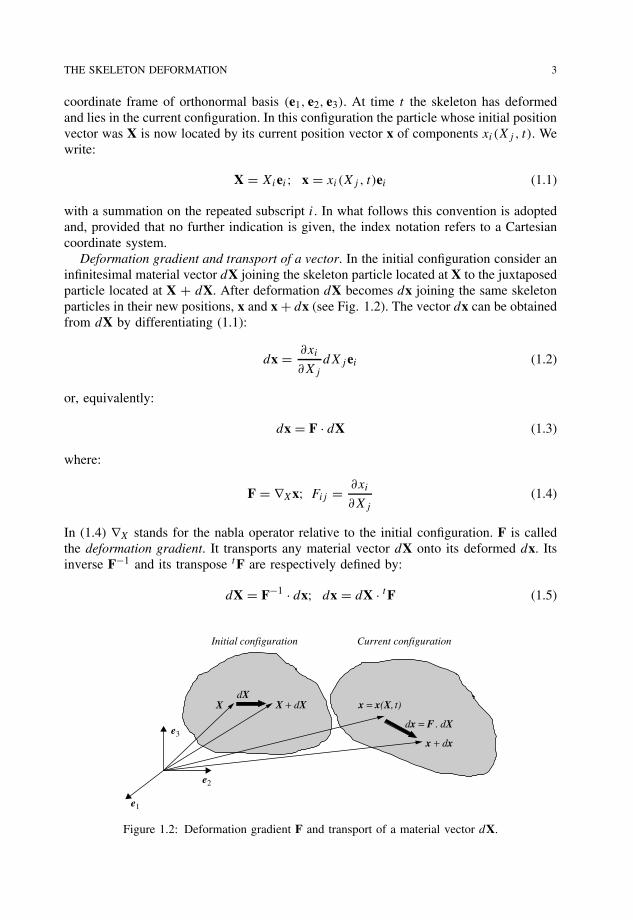
Deformation gradient and transport of a vector. In the initial configuration consider aninfinitesimal material vector dX joining the skeleton particle located at X to the juxtaposedparticle located at X + dX. After deformation dX becomes dx joining the same skeletonparticles in their new positions, x and x + dx (see Fig. 1.2). The vector dx can be obtainedfrom dX by differentiating (1.1):

dx = ∂xi

∂Xj

dXj ei (1.2)

or, equivalently:

dx = F · dX (1.3)

where:

F = ∇Xx; Fij = ∂xi

∂Xj

(1.4)

In (1.4) ∇X stands for the nabla operator relative to the initial configuration. F is calledthe deformation gradient. It transports any material vector dX onto its deformed dx. Itsinverse F−1 and its transpose tF are respectively defined by:

dX = F−1 · dx; dx = dX · tF (1.5)

e2

e3

e1

x = x(X, t)XdX

dx = F . dX

Initial configuration Current configuration

X + dX

x + dx

Figure 1.2: Deformation gradient F and transport of a material vector dX.


and satisfy:

(tF)ij = Fji; (F−1)ij = ∂Xi

∂xj

(1.6)

Deformation gradient and displacement. Let ξ (X, t) be the displacement vector of theparticle whose initial and current positions are X and x. We write:

x = X + ξ (1.7)

From definitions (1.4) and (1.7) deformation gradient F can be expressed as a functionof displacement vector ξ according to:

F = 1 + ∇Xξ ; Fij = δij + ∂ξi

∂Xj

(1.8)

where δij is the Kronecker delta, that is δij = 1 if i = j and δij = 0 if i = j .Volume transport. The current infinitesimal volume dt = dx1 dx2 dx3 is equal to the

composed product:

dt = (dx1, dx2, dx3) = dx1 · (dx2 × dx3) (1.9)

where dxi = dxi ei (with no summation). The linearity of the composed product withrespect to the vectors it combines allows us to write:

dt = (F · dX1, F · dX2, F · dX3) = det F (dX1, dX2, dX3) (1.10)

As a consequence any initial material volume d0 transforms into the material volumedt through the relation:

dt = Jd0 (1.11)

where J = det F is the Jacobian of the deformation.Surface transport. Consider a material surface dA, oriented by the unit normal N.

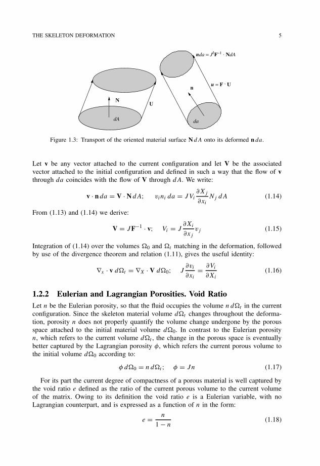
Throughout the deformation dA transforms into the material surface da, oriented by theunit normal n. Since vectors N and n are not material vectors, they do not match in thedeformation. Let U be any material vector in the initial configuration. The material cylinderof initial volume N · U dA transforms into the material cylinder of volume n · F · U da

(see Fig. 1.3). According to (1.11) we write:

n · F · U da = J N · U dA (1.12)

Since (1.12) holds whatever the vector U, we derive:

n da = J tF−1 · N dA; ni da = J∂Xj

∂xi

Nj dA (1.13)


U

dA

u = F . U

da

N

n

nda = JtF−1 . NdA

Figure 1.3: Transport of the oriented material surface N dA onto its deformed n da.

Let v be any vector attached to the current configuration and let V be the associatedvector attached to the initial configuration and defined in such a way that the flow of vthrough da coincides with the flow of V through dA. We write:

v · n da = V · N dA; vini da = JVi

∂Xj

∂xi

Nj dA (1.14)

From (1.13) and (1.14) we derive:

V = JF−1 · v; Vi = J∂Xi

∂xj

vj (1.15)

Integration of (1.14) over the volumes 0 and t matching in the deformation, followedby use of the divergence theorem and relation (1.11), gives the useful identity:

∇x · v dt = ∇X · V d0; J∂vi

∂xi

= ∂Vi

∂Xi

(1.16)

1.2.2 Eulerian and Lagrangian Porosities. Void RatioLet n be the Eulerian porosity, so that the fluid occupies the volume n dt in the currentconfiguration. Since the skeleton material volume dt changes throughout the deforma-tion, porosity n does not properly quantify the volume change undergone by the porousspace attached to the initial material volume d0. In contrast to the Eulerian porosityn, which refers to the current volume dt , the change in the porous space is eventuallybetter captured by the Lagrangian porosity φ, which refers the current porous volume tothe initial volume d0 according to:

φ d0 = n dt ; φ = Jn (1.17)

For its part the current degree of compactness of a porous material is well captured bythe void ratio e defined as the ratio of the current porous volume to the current volumeof the matrix. Owing to its definition the void ratio e is a Eulerian variable, with noLagrangian counterpart, and is expressed as a function of n in the form:

e = n

1 − n(1.18)


1.2.3 Strain Tensor

Deformation induces changes in both the lengths of the material vectors and the anglesbetween them. The Green–Lagrange strain tensor measures these changes by quanti-fying the variation of the scalar product of two material vectors dX and dY transformingthe deformation throughout into dx and dy. We write:

dx = F · dX; dy = F · dY : dx · dy − dX · dY = 2dX · · dY (1.19)

With the help of (1.5) can be written as a function of deformation gradient Faccording to:

= 1

2(tF · F − 1) (1.20)

Being symmetric, tensor admits three real eigenvalues J (J = I, II, III ). The latterare the principal strains and are associated with the eigenvectors eJ (J = I, II, III ),which are the principal directions of the deformation such as · eJ = J eJ . The orthog-onality of the principal directions, writing eI · eJ = 0, is preserved in the deformation.Indeed: (

eI · tF) · (F · eJ ) = 2eI · · eJ = 2I or J eI · eJ = 0 (1.21)

The gradient R of the rotation that rigidly transports the set of orthogonal principaldirections eJ to their final directions is an isometry so that the related strain tensoris zero, resulting in tR = R−1. Therefore the gradient F of any transformation decom-poses as:

F = D · R (1.22)

that is the rotation R followed by the actual deformation D, the latter involving no rota-tion and matching the dilation of the principal directions of deformation. Equivalently,the gradient F can also decompose as the actual deformation D′ matching the dilation,followed by the rotation R′ relative to that of the eigenvectors. Accordingly, the straintensor accounts entirely for the actual deformation since:

= 1

2(D2 − 1) (1.23)

By means of (1.8) can finally be expressed as a function of the displacement vector ξ

according to:

= 1

2

(∇Xξ + t∇Xξ + t∇Xξ · ∇Xξ)

(1.24a)

ij = 1

2

(∂ξi

∂Xj

+ ∂ξj

∂Xi

+ ∂ξk

∂Xi

∂ξk

∂Xj

)(1.24b)


1.2.4 Infinitesimal Transformation and the Linearized Strain TensorIn many problems a first-order approximation to the finite theory can be carried out underthe condition of infinitesimal transformation, that is

‖∇ξ‖ 1 (1.25)

where the norm ‖(·)‖ of (·) has not been specified because of the equivalence of all thenorms in a vectorial space of finite three dimensions. Moreover, as far as only spatialderivations are concerned, in the limit of infinitesimal transformation the current and theinitial configurations merge, so the nabla operator ∇ can be used with no need for asubscript referring to a particular configuration, that is ∇ = ∇X ≡ ∇x .

Under condition (1.25) the Green–Lagrange strain tensor reduces to the linearizedstrain tensor ε:

ε = 1

2(∇ξ + t∇ξ); εij = 1

2

(∂ξi

∂xj

+ ∂ξj

∂xi

)(1.26)

Since has the same order of magnitude as ∇Xξ , infinitesimal transformation impliesinfinitesimal deformation, that is ‖‖ 1. In contrast, the deformation may be infinites-imal whereas the transformation is not. For instance, in a rigid body motion is zerowhereas ∇Xξ can have any order of magnitude.

Under the approximation of infinitesimal transformation, (1.8) gives:

(J = det F) (

1 + ∇ · ξ = 1 + ∂ξi

∂xi

= 1 + εii

)(1.27)

From now on let ε be the linearized volume dilation of the skeleton, that is:

ε = εii = ∇ · ξ (1.28)

so that (1.11) takes the form:

dt (1 + ε) d0 (1.29)

The observable macroscopic volume dilation undergone by the skeleton is due bothto the change in porosity and to the volume dilation εs undergone by the solid matrix,although the latter is not accessible from purely macroscopic experiments. Analogouslyto (1.29) the definition of εs allows us to write:

dst = (1 + εs) ds

0 (1.30)

Owing to the respective definition of Eulerian and Lagrangian porosities, n and φ (see§1.2.2), the volume occupied by the matrix is linked to the overall volume through therelations:

dst = (1 − n) dt = dt − φ d0; ds

0 = (1 − φ0) d0 (1.31)


Combining the above equations, we finally derive the volume balance:

ε = (1 − φ0)εs + φ − φ0 (1.32)

In the absence of any occluded porosity, the solid grains forming the matrix generallyundergo negligible volume changes so that the matrix can be considered as incompressible.Accordingly we let εs = 0 in (1.32), giving:

ε = φ − φ0 (1.33)

As is usually done in soil mechanics, it can be more convenient to use the void ratio e

instead of the volumetric dilation ε. Combining (1.17), (1.18) and (1.33), we obtain:

ε = e − e0

1 + e0(1.34)

Under the approximation of infinitesimal transformation, the diagonal term εii (with nosummation) is equal to the linear dilation in the ei direction, while twice the non-diagonalterm, γij = 2εij (i = j ), is equal to the distortion related to directions ei and ej , that isthe change undergone by the angle made between the material vectors ei and ej that werenormal prior to the deformation.

1.3 Kinematics

The description of the skeleton deformation by means of the deformation gradient F is bynature a Lagrangian description. The fields are functions of time t and of position vectorX locating the skeleton particle in the initial configuration. The latter does not vary withtime and the kinematics of the skeleton results from a simple time derivation.

In contrast to the Lagrangian approach, the Eulerian approach involves only the currentconfiguration, with no reference to any initial configuration. The approach is carried outby using the velocity field Vπ(x, t) of the particle coinciding at time t with the geometricalpoint located at x. The particle can be either a skeleton particle, π = s, or a fluid particle,π = f .1 At time t , the same Eulerian approach applies to both particles since the skeletoncontinuum and the fluid continuum merge in the same current configuration.

1.3.1 Particle Derivative

Definition

The particle derivative dπG/dt with respect to particle π (= s or f ) of some field G is thetime derivative of G that an observer attached to the particle would derive. This observerrecords the variation dπG of quantity G between times t and t + dt . For instance, the

1It would have been more rigorous to make a distinction between the index referring to the matter at themacroscopic scale (for instance, sk for the skeleton particle and f l for the fluid particle) and the index referringto the matter at the mesoscopic scale (for instance, s for the solid matrix, as in (1.32), and f for the fluid).However, for the sake of simplicity of notation, we chose not to make this distinction.

KINEMATICS 9

origin of the coordinate being fixed, the velocity field Vπ (x, t) of particle π located at xreads:

dπxdt

= Vπ(x, t); π = s or f (1.35)

Particle derivative of a material vector

Definition (1.35) allows us to write the particle derivative of the material vector dx in theform:

dπ

dt(dx) = dπ

dt[(x+dx) − x] = Vπ (x+dx, t) − Vπ (x, t) (1.36)

so that:

dπ

dt(dx) = ∇xVπ · dx; (∇xVπ

)ij

= ∂V πi

∂xj

; π = s or f (1.37)

Particle derivative of a material volume

Starting from (1.9), we express the particle derivative of the material volume dt in theform:

dπ

dt(dt ) = dπ

dt(dx1, dx2, dx3) = dπ

dt(dx1 · (dx2 × dx3)) (1.38)

The linearity of the composed product (v1, v2, v3) with regard to vectors vi=1,2,3 allowsus to write:

dπ

dt(dt ) =

(dπ

dt(dx1), dx2, dx3

)

+(

dx1,dπ

dt(dx2), dx3

)+

(dx1, dx2,

dπ

dt(dx3)

)(1.39)

Use of (1.37) gives:

dπ

dt(dt ) =

(∂V π

i

∂x1ei dx1, dx2, dx3

)

+(

dx1,∂V π

i

∂x2ei dx2, dx3

)+

(dx1, dx2,

∂V πi

∂x3ei dx3

)(1.40)

The product (v1, v2, v3) is zero as soon as two vectors among vectors vi=1,2,3 are colin-ear. Thus:

dπ

dt(dt ) =

(∂V π

1

∂x1+ ∂V π

2

∂x2+ ∂V π

3

∂x3

)(dx1, dx2, dx3) (1.41)

or equivalently:

dπ

dt(dt ) = (∇x · Vπ

)dt ; π = s or f (1.42)


Particle derivative of a field

The particle derivative dπG/dt with respect to particle π (= s or f ) of field G (x, t) turnsout to be the time derivative of G when letting x match the successive positions xπ (t)

occupied by the particle. We write:

dπGdt

= ∂G∂t

+ (∇xG) · Vπ (1.43)

For instance, the acceleration γ π of particle π is the particle derivative of velocityVπ (x, t):

γ π = dπVπ

dt= ∂Vπ

∂t+ (∇xVπ

) · Vπ ; γ πi = ∂V π

i

∂t+ ∂V π

i

∂xj

V πj (1.44)

Particle derivative of a volume integral

The particle derivative applies to the volume integral of any quantity G according to:

dπ

dt

∫t

Gdt =∫

t

dπ

dt(Gdt) (1.45)

Use of (1.42) and (1.43) allows us to rewrite (1.45) in the form:

dπ

dt

∫t

Gdt =∫

t

(dπGdt

+ G∇x · Vπ

)dt (1.46)

or, equivalently:

dπ

dt

∫t

Gdt =∫

t

(∂G∂t

+ ∇x · (GVπ)

)dt (1.47)

Use of the divergence theorem finally provides the alternative expression:

dπ

dt

∫t

Gdt =∫

t

∂G∂t

dt +∫

∂t

GVπ · n da (1.48)

where ∂t stands for the border of volume t , while n is the outward unit normal tosurface da.

1.3.2 Strain Rates

The particle derivative allows the Eulerian description of the kinematics of the deformationthat refers only to the current configuration. The Eulerian strain rate tensor dπ is definedby the relation:

dπ

dt(dx · dy) = 2dx · dπ · dy (1.49)

KINEMATICS 11

where dx and dy are any infinitesimal skeleton (π = s) or fluid (π = f ) material vectors.Use of (1.37) into (1.49) gives:

dπ = 1

2

(∇xVπ + t∇xVπ); dπ

ij = 1

2

(∂V π

i

∂xj

+∂V π

j

∂xi

)(1.50)

Definition (1.50) of dπ allows us to decompose the deformation kinematics of materialvector dx in the form:

dπ

dt(dx) = π · dx + dπ · dx (1.51)

where π is the rotation rate tensor attached to the antisymmetric part of ∇xVπ :

π = 1

2

(∇xVπ − t∇xVπ); π

ij = 1

2

(∂V π

i

∂xj

−∂V π

j

∂xi

)(1.52)

The term π · dx in (1.51) induces no strain rate since it accounts for the infinitesimalrotation of material vector dx according to:

π · dx = 2ωπ × dx (1.53)

where ωπ is the vorticity vector:

ωπ = ∇x × Vπ (1.54)

The Eulerian decomposition (1.51) of the kinematics of deformation is to be comparedwith the Lagrangian decomposition (1.22) of the deformation.

In contrast to the Eulerian approach to the kinematics of the skeleton deformation, theLagrangian approach consists in deriving (1.19) with respect to time:2

ds

dt(dx · dy) = 2dX · d

dt· dY (1.55)

Using transport formulae dx = F · dX and dy = F · dY, the comparison between (1.49)for π = s and (1.55) leads to the transport formula:

ds = tF−1 · d

dt· F−1; ds

ij = ∂Xk

∂xi

dkl

dt

∂Xl

∂xj

(1.56)

According to (1.26) and (1.56), the infinitesimal transformation approximation turns outto consider ds dε/dt .

2When taking the skeleton particle derivative of Lagrangian quantities, as for instance ds/dt , we willadopt a standard time derivative notation, such as for instance d/dt in (1.55). Indeed, there is no ambiguitysince = (X, t). Furthermore, the particle derivative with respect to the fluid of a Lagrangian quantity doesnot generally present any physical interest.


1.4 Mass Balance

1.4.1 Equation of Continuity

Let ρs and ρf be the mesoscopic or intrinsic matrix and fluid mass densities so thatρs (1 − n) dt and ρf n dt are respectively the skeleton mass and the fluid mass cur-rently contained in the material volume dt . Accordingly the macroscopic or apparentskeleton and fluid mass densities are respectively ρs (1 − n) and ρf n. When no masschange occurs, neither for the skeleton nor the fluid contained in the volume t , the massbalance can be expressed in the form:

ds

dt

∫t

ρs (1 − n) dt = 0 (1.57a)

df

dt

∫t

ρf n dt = 0 (1.57b)

Applying (1.45) and (1.47) to (1.57) we get:

ds

dt(ρs (1 − n) dt) = 0 (1.58a)

df

dt(ρf n dt) = 0 (1.58b)

and the Eulerian continuity equations:

∂(ρs (1 − n))

∂t+ ∇x · (ρs (1 − n) Vs

) = 0 (1.59a)

∂(ρf n)

∂t+ ∇x · (ρf nVf

) = 0 (1.59b)

1.4.2 The Relative Flow Vector of a Fluid Mass. Filtration Vector.Fluid Mass Content

The appropriate formulation of the constitutive equations for the skeleton accounting forthe skeleton–fluid couplings will require referring the motion of the fluid to the initialconfiguration of the skeleton. With that purpose in mind let Jf da be the fluid massflowing between time t and t + dt through the infinitesimal skeleton material surface da

oriented by the unit normal n. We write:

Jf da = w · n da (1.60)

where w (x, t) is the Eulerian relative flow vector of fluid mass. Since the quantity n(Vf −Vs) · n dadt is the infinitesimal fluid volume flowing through the skeleton surface da

during the infinitesimal time dt (see Fig. 1.4), the relative vector of fluid mass w isconsistently defined by:

w = ρfV; V = n(Vf − Vs) (1.61)

MASS BALANCE 13

(Vf − Vs) dt

n (Vf − Vs) . n dadt

nda

Figure 1.4: The infinitesimal fluid volume flowing through the skeleton surface da during theinfinitesimal time dt . Eulerian porosity n is still to be associated with the infinitesimal fluid volume(Vf − Vs

) · n dadt , and not with the skeleton infinitesimal surface da through which the fluidflows.

where V is the filtration vector. Use of definition (1.61) allows us to refer the fluid massbalance to the skeleton motion by rearranging the fluid continuity equation (1.59b) in theform:

ds(ρf n)

dt+ ρf n∇x · Vs+∇x · w = 0 (1.62)

The Lagrangian approach to the fluid mass balance can be carried out by introducingthe current Lagrangian fluid mass content mf per unit of initial volume d0. The latterrelates to the current Eulerian fluid mass content ρf n per unit of current volume dt

according to:

ρf n dt = mf d0 (1.63)

Use of (1.17) and (1.63) gives the useful relation:

mf = ρf φ (1.64)

where φ stands for the Lagrangian porosity (see §1.2.2). Furthermore, let M (X, t) be theLagrangian vector attached to the initial configuration and linked to vector w through therelation:

w · n da = M · N dA (1.65)

where surfaces da and dA correspond in the skeleton deformation. Accordingly, lettingw = v and M = V in (1.14), Eqs. (1.15) and (1.16) provide the transport formulae:

M = JF−1 · w; ∇x · w dt = ∇X · M d0 (1.66a)

Mi = J∂Xi

∂xj

wj ; J∂wi

∂xi

= ∂Mi

∂Xi

(1.66b)


Substitution of (1.63) and (1.66) into (1.62) premultiplied by dt , and use of (1.42) withπ = s, provide the Lagrangian fluid continuity equation in the form:

dmf

dt+ ∇X · M = 0; ∂mf (X, t)

∂t+ ∂Mi

∂Xi

= 0 (1.67)

Analogously, the Lagrangian approach to the mass balance of the skeleton turns out tointegrate (1.58a) in the form:

ρs (1 − n) dt = ρ0s (1 − n0)d0 (1.68)

where ρ0s and n0 = φ0 stand respectively for the initial matrix mass density and for the

initial porosity. Use of (1.11) allows us to write:

ms = m0s = ρ0

s (1 − φ0) (1.69)

where ms = Jρs (1 − n) denotes the skeleton mass content per unit of initial volume d0and remains constantly equal to its initial value m0

s representing the skeleton mass densityρ0

s (1 − φ0). Equations (1.67) and (1.69) constitute the skeleton Lagrangian alternative tothe Eulerian continuity equations (1.59).

1.5 Advanced Analysis

1.5.1 Particle Derivative with a Surface of Discontinuity

Some applications involve propagation fronts across which discontinuities occur. In orderto derive the particle derivative of an integral accounting for these discontinuities, let

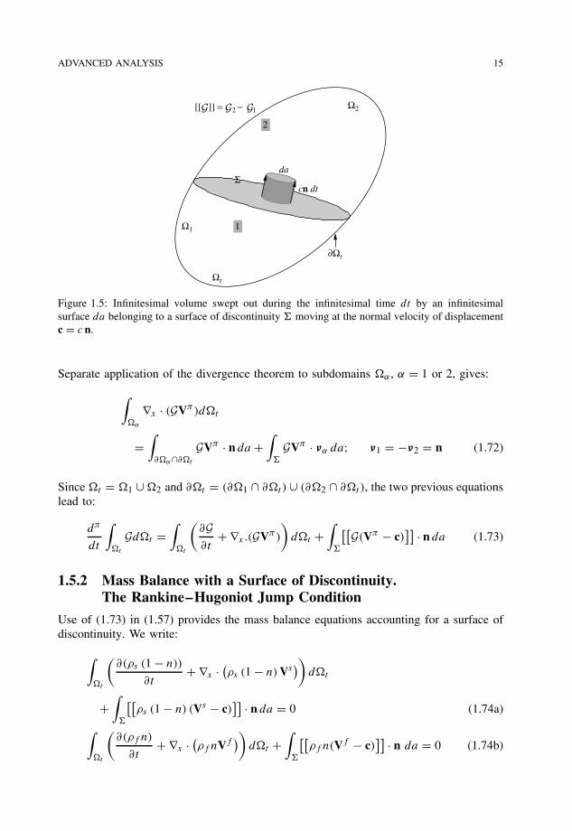
be a surface of discontinuity travelling within the material volume t and subdividingthe latter into two subvolumes 1 and 2. Let n be the unit normal to oriented in thedirection of travel towards the downstream subvolume 2. Finally, let [[G]] denote thejump across in the direction of n of the discontinuous quantity G (see Fig. 1.5):

[[G]] = G2 − G1 (1.70)

The normal speed of displacement c = c n of the surface of discontinuity is thevelocity at which a geometrical point belonging to moves along the normal n. During thetime duration dt the infinitesimal surface da belonging to sweeps out the infinitesimalvolume c · n da dt . During the infinitesimal time dt the volumetric density G related tothe latter undergoes the variation − [[G]]. In order to account for this sudden variation,the particle derivative of a volume integral (1.48) has to be modified according to:

dπ

dt

∫α

Gdt =∫

t

∂G∂t

dt +∫

∂t

GVπ · n da −∫

[[G]] c · n da (1.71)

ADVANCED ANALYSIS 15

2

1Ω1

Σda

cn dt

Ω2

Ωt

∂Ωt

[[ ]] = 2 − 1

Figure 1.5: Infinitesimal volume swept out during the infinitesimal time dt by an infinitesimalsurface da belonging to a surface of discontinuity moving at the normal velocity of displacementc = c n.

Separate application of the divergence theorem to subdomains α , α = 1 or 2, gives:

∫α

∇x · (GVπ)dt

=∫

∂α∩∂t

GVπ · n da +∫

GVπ · να da; ν1 = −ν2 = n (1.72)

Since t = 1 ∪ 2 and ∂t = (∂1 ∩ ∂t) ∪ (∂2 ∩ ∂t), the two previous equationslead to:

dπ

dt

∫t

Gdt =∫

t

(∂G∂t

+ ∇x.(GVπ)

)dt +

∫

[[G(Vπ − c)

]] · n da (1.73)

1.5.2 Mass Balance with a Surface of Discontinuity.The Rankine–Hugoniot Jump Condition

Use of (1.73) in (1.57) provides the mass balance equations accounting for a surface ofdiscontinuity. We write:

∫t

(∂(ρs (1 − n))

∂t+ ∇x · (

ρs (1 − n) Vs))

dt

+∫

[[ρs (1 − n) (Vs − c)

]] · n da = 0 (1.74a)

∫t

(∂(ρf n)

∂t+ ∇x · (ρf nVf

))dt +

∫

[[ρf n(Vf − c)

]] · n da = 0 (1.74b)


The first term in the above equations allows us to recover continuity equations (1.59),whereas the second term provides the jump or Rankine–Hugoniot conditions:

[[ρs (1 − n) (Vs − c)

]] · n = 0 (1.75a)[[ρf n(Vf − c)

]] · n = 0 (1.75b)

The jump condition means that the particles passing across the surface of discontinuity do not undergo any mass change. Referring to the skeleton motion, the jump condition(1.75b) relative to the fluid is conveniently rewritten in the form:

[[w − ρf n(c − Vs)

]] · n = 0 (1.76)

Let us apply the jump condition to the special case of a surface of discontinuity

constituted by the interface between two different porous media. Assuming that the twomedia are perfectly bonded, Vs remains continuous across their interface so that thedisplacement speed c = c · n equals the normal skeleton velocity Vs · n. Consequently, atthe interface of two bonded porous media, the jump condition (1.76), which eventuallyensures that no liquid filtration occurs along the interface, reduces to:

[[w]] · n = 0 (1.77)

During time dt the infinitesimal surface da belonging to the surface of discontinuity

sweeps out, in the current configuration, the skeleton material volume (c − Vs) · n da dt .In the meantime the infinitesimal surface dA associated with da through transport for-mula (1.13) sweeps out, in the initial configuration, the skeleton volume C · N dA dt .Lagrangian normal speed C is the speed at which a geometrical point belonging to thesurface of discontinuity moves between times t and t + dt in the reference configurationalong the normal N. By using (1.64) and (1.65), the Eulerian jump condition (1.76) canbe transported to the initial configuration to furnish the Lagrangian jump condition:

[[M − mf C

]] · N = 0 (1.78)

With the aim of giving a first illustration of the above Lagrangian approach to theRankine–Hugoniot jump condition (see §5.4.4 for a second illustration), let us considera porous material subjected to a dissolution process (e.g. of leaching type, see §7.1), inwhich the solid matrix (e.g. calcium) progressively dissolves into the interstitial solutionfilling the porous space. At the microscopic scale of the latter, the problem at hand involvesthe propagation of a surface of discontinuity in the initial configuration, even though thedissolution front representing the surface of discontinuity in the current configurationremains constantly identified with the current internal walls of the porous space. At themicroscopic scale we apply (1.78) in the form:

(M − mC) · Nintact = (M − mC) · Nsolute (1.79)

where, for the sake of simplicity, we retain the same notation as that used at the macro-scopic scale: M represents the Lagrangian relative flux vector with respect to the solid

ADVANCED ANALYSIS 17

matrix; m is the total mass per unit of initial volume of the species subjected to disso-lution; C = C · N is the Lagrangian speed of propagation front , which separates, inthe initial configuration the still intact zone from the already dissolved one. The aboveequation eventually expresses the mass conservation related to the thin layer of solidmatrix currently passing from the intact state, as part of the solid matrix, to the dissolvedstate, as contributing to the solute. On the intact side we write M = 0 and m = m0 sincethe still intact material, that is the current solid matrix, has no relative motion with respectto itself. Returning to the macroscopic scale, let dφch/dt be the chemical contribution tothe total rate dφ/dt of Lagrangian porosity, that is the one due only to the dissolutionprocess irrespective of strain effects. According to the above analysis, dφch/dt can beexpressed in the form:

dφch

dt= 1

d0

∫

CdA (1.80)

1.5.3 Mass Balance and the Double Porosity Network

Some materials such as rocks or concrete sometimes exhibit two very distinct porousnetworks. Roughly speaking, the first is formed of rounded pores, while the second isformed of penny-shaped cracks. Although these two networks can exchange fluid massbetween them, their quite different geometries result in distinct evolution laws of theirpore pressure and require a separate analysis. To this end let subscript 1 refer to theporous network formed of cracks and subscript 2 to the one formed of pores. While thecontinuity equation related to the skeleton remains unchanged, the fluid mass balancenow reads:

df1

dt

∫t

ρf1n1 dt =∫

t

r2→1 dt (1.81a)

df2

dt

∫t

ρf2n2 dt =∫

t

r1→2 dt (1.81b)

whererα→β stands for the rate of fluid mass flowing from network α into network β,

while nα is the porosity associated with network α so that n = n1 + n2.Mass conservation requires

rα→β = −

rβ→α and application of (1.45) to (1.81) gives:

df1

dt(ρf1n1 dt) = −

r1→2 dt ; df2

dt(ρf2n2 dt) =

r1→2 dt (1.82)

Using (1.46), we obtain two separate continuity equations for the fluid flowing throughthe crack network and for the one flowing through the pore network:

∂(ρf1n1)

∂t+ ∇x · (ρf1n1Vf1

) = −r1→2 (1.83a)

∂(ρf2n2)

∂t+ ∇x · (ρf2n2Vf2

) = r1→2 (1.83b)


The Lagrangian alternative to the previous Eulerian fluid continuity equations can bewritten as:

dsm1

dt+ ∇X · M(1) = −

m1→2 (1.84a)

dsm2

dt+ ∇X · M(2) =

m1→2 (1.84b)

with:

mα = Jρfαnα = ρfαφα; m1→2 = J

r1→2 (1.85)

The approach can be adapted in order to account for possible long-term exchangesof fluid mass between the occluded porosity, through which no fluid flow significantlyoccurs in the short-term range, and the connected porous network, through which the fluidflows at any time. This fluid exchange can be viewed as an exchange of mass betweenthe skeleton, including the occluded porosity and its fluid, and still referred to by s, andthe fluid saturating the porous network referred to by f . Analogously to (1.83) and (1.84)the Eulerian and Lagrangian approaches to the continuity equation respectively read:

∂(ρs (1 − n))

∂t+ ∇x · (ρs (1 − n) Vs

) = −rs→f (1.86a)

∂(ρf n)

∂t+ ∇x · (

ρf nVf) =

rs→f (1.86b)

and:

dsms

dt= −

ms→f (1.87a)

dsmf

dt+ ∇X · M =

ms→f (1.87b)

Similarly, consider a material subjected to a dissolution process. Letms→sol be the rate

of solid mass (index s) which currently dissolves per unit of initial volume d0 in soluteform (index sol), so that the mass conservation of the solid matrix, the solute and thesolvent (index w for liquid water) can be expressed in the form:

dsms

dt= −

ms→sol (1.88a)

dsmsol

dt+ ∇X · Msol =

ms→sol (1.88b)

dsmw

dt+ ∇X · Mw = 0 (1.88c)

In addition, from the analysis of §1.5.2 and from (1.80) we derive:

ms→sol = ρ0

s

dφch

dt(1.89)

Deformation and Kinematics. Mass Balancecatalogimages.wiley.com/images/db/pdf/0470849207.01.pdf ·...

Documents

Transcript of Deformation and Kinematics. Mass Balancecatalogimages.wiley.com/images/db/pdf/0470849207.01.pdf ·...