Chapter 2

Kinematics: Deformation and Flow

2.1 Introduction

We need a suitable mathematical framework in order to describe the behaviour of continua. Oureveryday experience tells us that lumps of matter can both move (change in position) and deform(change in shape), so we need to be able to quantify both these effects. Hopefully, you are alreadybe familiar with the kinematics of individual particles from basic mechanics. In classical particlemechanics, the position of the particle is described by a position vector r(t) measured from a chosenorigin in three-dimensional Euclidean space, �3 . The position is a function of one-dimensionalcontinuous time, t ∈ [0,∞), and contains all the information that we need to describe the motionof the particle.

Ω0

Ωt

r R

χt

e1

e2

e3

Figure 2.1: A region Ω0 is mapped to the region Ωt by the mapping χt which carries the materialpoint r ∈ Ω0 to the point R ∈ Ωt.

In continuum mechanics, we need to account for the motion of all the “particles” within thematerial. Consider a continuous body that initially occupies a region1 Ω0 of three-dimensionalEuclidean space �

3 , with volume V0 and surface ∂V0 ≡ S0. The body can be regarded as a

1If you want to get fancy you can call this an open subset.

32

collection of particles, called material points, each of which2 is described by a position vectorr = xKeK from our fixed origin in a Cartesian coordinate system3. We shall term the configurationΩ0 the undeformed configuration. At a later time t, the same body occupies a different regionof space, Ωt, with volume Vt and surface St. The material points within the region Ωt are nowdescribed by a position vector R = XKeK from the same origin in the same Cartesian coordinatesystem4. We shall term the configuration Ωt the deformed configuration, see Figure 2.1.

The change in configuration from Ω0 to Ωt can be described by a function χt : Ω0 → Ωt,sometimes called a deformation map. The position at time t is given by R = χt(r) ≡ χ(r, t),where χ : Ω0 × [0,∞) → Ωt is a continuous map. In other words, each material point5 in theundeformed configuration Ω0 is carried to a (material) point in the deformed configuration Ωt.

On physical grounds, we expect that (a) matter cannot be destroyed and (b) matter does notinterpenetrate. A deformation map will be consistent with these conditions if it is one-to-one andthe Jacobian of the mapping remains non zero. The Jacobian of the mapping is the determinant ofthe matrix, F = ∇

rχt, (note that the gradient is taken with respect to the undeformed coordinates

r) whose components in the Cartesian basis are given by

FIJ =∂XI

∂xJ

, (2.1)

and so our physical constraints demand that

det F 6= 0. (2.2)

In fact, we impose the stronger condition that the Jacobian of the mapping remains positive, whichensures that material lines preserve their relative orientations: a body cannot be deformed onto itsmirror image. If condition (2.2) is satisfied then a (local) inverse mapping can be constructed thatgives the initial position as a function of the current position, r = χ−1

t (R) ≡ χ−1(R, t).

Example 2.1. An example deformationIs the mapping given by

χ(x) :

(χ1 = 2x1 + 3x2,

χ2 = 1x1 + 2x2.

physically admissible? If so, sketch the deformed unit square xI ∈ [0, 1] that follows after applicationof the mapping.

Solution 2.1. The deformed position is given by�

X1

X2

�=

�2 31 2

��x1

x2

�,

and det F = 2 × 2 − 3 × 1 = 1 > 0, so the mapping is physically admissible. The deformed unitsquare can be obtained by thinking about the deformation of the corners and the knowledge that

2We could label the position vector r by another index to distinguish different material points, but the notationis less cumbersome if we treat each specific value of r as the definition of the different material points.

3Even when we consider non-Cartesian coordinates later, it’s easiest to define those coordinates relative to thefixed Cartesian system. Note that because this is a Cartesian coordinate system we have not bothered to indicatethe contravariant nature of the components.

4For further generality, we should assume a different orthonormal coordinate system for the deformed configurationR = XK eK , but the notation becomes even more cluttered without really aiding understanding.

5From the classical particle mechanics viewpoint, there is a single material point (the particle) with positionvector x(t) = R = χt(r) = χt(x(0)).

the deformation is homogeneous (the matrix entries are not themselves functions of x). The cornersmap as follows

(0, 0) → (0, 0); (1, 0) → (2, 1); (0, 1) → (3, 2); (1, 1) → (5, 3),

and the undeformed and deformed regions are shown in Figure 2.2.

e1

e2

Figure 2.2: A unit square (solid boundary) is deformed into a quadrilateral region (dashed boundary)by the mapping χ.

2.2 Lagrangian (Material) and Eulerian (Spatial) Descrip-

tions

Given the existence of the continuous mapping χ, we can write (each Cartesian coordinate of) amaterial point in the deformed position as a function of (the Cartesian coordinates of) the samematerial point in the undeformed position and the time t,

XK(t) = χ(xJ , t)·eK , which we can write in vector form as R(r, t). (2.3)

In equation (2.3) the current position is treated as a function of the original position, which is theindependent variable. This is called a Lagrangian or material description. Any other fields are alsotreated as functions of the original position. In the Lagrangian description, we follow the evolutionof particular material particles with time6. It is more common to use a Lagrangian descriptionin solid mechanics where the initial undeformed geometry is often simple, but the deformationsbecome complex.

Alternatively, we could use the inverse mapping to write (each Cartesian coordinates of) theundeformed position of a material point as a function of (the Cartesian coordinates of) its currentposition

xK(t) = χ−1(XJ , t)·eK , or r(R, t). (2.4)

Here, the current position is the independent variable and this is called an Eulerian or spatialdescription. Any other fields are treated as functions of the fixed position R. In the Eulerian

6The Lagrangian description is the viewpoint used in classical particle mechanics because we are only interestedin the behaviour of each individual particle.

description, we observe the changes over time at a fixed point in space7. It is more common to usean Eulerian description in fluid mechanics, if the original location of particular fluid particles is notof interest.

The transformation of an object from an Eulerian (current) description to the Lagrangian (ref-erence) description is sometimes called a pullback (terminology taken from differential geometry).The converse operation of transforming from the Lagrangian to the Eulerian description is called apushforward.

For simplicity, we have defined the deformed and undeformed positions in the same globalCartesian coordinate system, but this is not necessary. It is perfectly possible to use differentcoordinate systems to represent the deformed and undeformed positions, which may be usefulin certain special problems: e.g. a cube being deformed into a cylinder. However, the use ofgeneral coordinates would bring in the complication of covariant and contravariant transformations.We shall consider general curvilinear coordinates in what follows after the initial development inCartesians. The curvilinear coordinates associated with the Lagrangian viewpoint will be denotedby ξi and those in the Eulerian χi.

2.3 Displacement, Velocity and Acceleration

Newton’s laws of mechanics were originally formulated for individual particles and the displacement,velocity and acceleration of each particle are derived from its position as a function of time. Incontinuum mechanics we must also define these quantities based on the position of each materialpoint as a function of time (the Lagrangian viewpoint), but we can then reinterpret them as functionsof the absolute spatial position (the Eulerian viewpoint) if more convenient.

2.3.1 Displacement

The change in position of a material point within the body between configurations Ω0 and Ωt isgiven by the displacement vector field

u = R− r, (2.5)

which can be treated as a function of either R or r; i.e. from the Eulerian or Lagrangian viewpoints,respectively. For consistency of notation we shall write U(R, t) = R−r(R, t) for the displacementin the Eulerian representation and u(r, t) = R(r, t)− r in the Lagrangian.

Example 2.2. Displacement of a moving blockA block of material that initially occupies the region r ∈ [0, 1]× [0, 1]× [0, 1] moves in such a waythat its position is given by

R(r, t) = r(1 + t), (2.6)

at time t ≥ 0. Find the displacement of the block in both the Eulerian and Lagrangian representa-tions.

7The Eulerian description makes little sense in classical particle mechanics because in general motion the particleis unlikely to be located at our chosen fixed position for very long. Imagine trying to throw a ball in front of afixed (Eulerian) video camera: the ball will only appear on a short section of the video, or not at all if we do notthrow accurately. The reason why an Eulerian view makes more sense in continuum mechanics is that some part ofthe continuum will generally be located at our chosen fixed point, but exactly which part (which material points)changes with time.

Solution 2.2. We are given the relationship R(r, t), so the displacement in the Lagrangian view-point is straightforward to determine

u(r, t) = R(r, t)− r = tr.

For the Eulerian viewpoint, we need to invert the relationship (2.6) which gives r = R/(1 + t) andtherefore the displacement is

U(R, t) =t

1 + tR.

A potential problem with the Eulerian viewpoint is that it does not actually make sense unlessthe point R is within the body at time t.

2.3.2 Velocity

The velocity of a material point is the rate of change of its displacement with time. The Lagrangian(material) coordinate of each material point remains fixed, so the velocity, v, in the Lagrangianrepresentation is simply

v(r, t) =∂u(r, t)

∂t

����r fixed

=∂(R(r, t)− r)

∂t

����r=

∂R(r, t)

∂t

����r, (2.7)

because r is held fixed during the differentiation8. Note that the velocity moves with the materialpoints, which is exactly the same as in classical particle mechanics.

In the Eulerian framework, the velocity must be defined as a function of a specific fixed point inspace. The problem is that different material points will pass through the chosen spatial point atdifferent times. Thus, the Eulerian velocity must be calculated by finding the material coordinatethat corresponds to the fixed spatial location at chosen instant in time, r(R, t), so that

V (R, t) =∂U (R, t)

∂t

����r=

∂R

∂t

����r= v(r(R, t), t). (2.8)

Example 2.3. Calculation of the velocity for a rotating blockA cube of material that initially occupies the region r ∈ [−1, 1]× [−1, 1]× [−1, 1] rotates about thex3-axis with constant angular velocity so that its position at time t is given by

X1

X2

X3

=

cos t sin t 0− sin t cos t 0

0 0 1

x1

x2

x3

. (2.9)

Calculate both the Lagrangian and Eulerian velocities of the block.

Solution 2.3. The Lagrangian velocity is simple to calculate

v(r, t) =∂R

∂t, ⇒

v1v2v3

=

− sin t cos t 0− cos t − sin t 0

0 0 0

x1

x2

x3

, (2.10)

which is, as expected, the same as the velocity of a particle initially at (x1, x2) rotating about theorigin in the x1 − x2 plane.

8This is indicated by the vertical bar next to the partial derivative, which should not be confused with thecovariant derivative.

In order to convert to the Eulerian viewpoint we need to find r(R), which follows after inversionof the relationship (2.9):

x1

x2

x3

=

cos t − sin t 0sin t cos t 0

0 0 1

X1

X2

X3

. (2.11)

Thus the Eulerian velocity V (R, t) = v(r(R, t), t) is obtained by substituting the relationship(2.11) into the expression for the Lagrangian velocity (2.10)

V1

V2

V3

=

− sin t cos t 0− cos t − sin t 0

0 0 0

cos t − sin t 0sin t cos t 00 0 1

X1

X2

X3

=

0 1 0−1 0 00 0 0

X1

X2

X3

=

X2

−X1

0

,

which remains constant. In other words the velocity of the rotating block at a fixed point in space isconstant. Different material points pass through our chosen point but the velocity of each is alwaysthe same when it does so.

2.3.3 Acceleration

The acceleration of a material point is the rate of change of its velocity with time. Once again,computing the acceleration in the Lagrangian representation is very simple

a(r, t) =∂v(r, t)

∂t

����r=

∂2u(r, t)

∂t2

����r=

∂2R(r, t)

∂t2

����r. (2.12)

In the Eulerian framework, the velocity at a fixed point in space can change through two differentmechanisms: (i) the material velocity changes with time; or (ii) the material point (with a specificvelocity) is carried past the fixed point in space. The second mechanism is a consequence of themotion of the continuum and is known convection or advection. The two terms arise quite naturallyin the computation of the material acceleration at a fixed spatial location because for a fixed materialcoordinate, the position R is also a function of time

A(R, t) =∂V (R, t)

∂t

����r=

∂V (R(r, t), t)

∂t

����r. (2.13)

After application of the chain rule, equation (2.13) becomes

A(R, t) =∂V

∂t

����R

+∂V

∂R

����t

·∂R

∂t

����r=

∂V

∂t

����R

+ V ·∂V

∂R

����t

=∂V

∂t+ V · ∇

RV , (2.14)

or in component form

AI(R, t) =∂VI

∂t+ VJ

∂VI

∂XJ

. (2.15)

Note that the gradient is taken with respect to the Eulerian (deformed) coordinates R. The firstterm ∂V /∂t corresponds to the mechanism (i) above, whereas the second term V · ∇

RV corresponds

to the mechanism (ii) and is the advective term. The advective term is nonlinear in V , which leadsto many of the complex phenomena observed in continua9.

9Note that this nonlinearity only arises when observations are made in the Eulerian viewpoint, so it is definitelyobserver dependent.

2.3.4 Material Derivative

The argument used to determine the acceleration is rather general and can be used to define the ratesof change of any property that is carried with the continuum. For a scalar field φ(r, t) = Φ(R(r, t), t)the material derivative is the rate of change of the quantity keeping the Lagrangian coordinate r

fixed. The usual notation for the material derivative is Dφ/Dt and in the Lagrangian framework,the material derivative and the partial derivative coincide

Dφ

Dt=

∂φ

∂t(2.16)

In the Eulerian framework, however,

DΦ

Dt=

∂Φ

∂t+

∂Φ

∂XK

∂XK

∂t=

∂Φ

∂t+ VK

∂Φ

∂XK=

∂Φ

∂t+ V ·∇

RΦ. (2.17)

Curvilinear coordinates

If we use general (time-independent) curvilinear coordinates χi as as Eulerian coordinates, thenR(χi) and equation (2.17) becomes

Dφ

Dt=

∂φ

∂t+

∂φ

∂χi

∂χi

∂XK

∂XK

∂t=

∂φ

∂t+

∂χi

∂XK

VK∂φ

∂χi=

∂φ

∂t+ V i ∂φ

∂χi,

where we have use equation (1.16b) to determine the components V i in the covariant basis corre-sponding to the coordinates χi. The velocity vector is V = V iGi, where Gi = ∂R/∂χi are thecovariant base vectors in the deformed position with respect to Eulerian curvilinear coordinates χi.It follows that the acceleration in the Eulerian framework in general coordinates is given by

D(V jGj)

Dt=

∂(V jGj)

∂t+ V i

∂(V jGj)

∂χi.

Assuming that the base vectors are fixed in time, which is to be expected for a (sensible) Euleriancoordinate system, we obtain

DV

Dt=

∂V i

∂t+ V jV i||j

!Gi,

where here ||j indicates covariant differentiation in the Eulerian viewpoint with respect to the

Eulerian coordinates χi, i.e. using the the metric tensor Gi j = Gi·Gj . As you would expect, thisis simply the tensor component representation of the expression

DV

Dt=

∂V

∂t+ V · ∇

RV ;

a coordinate-system-independent vector expression.

2.4 Deformation

Thus far, we have considered the extension of concepts in particle mechanics, displacement, velocityand acceleration, to the continuum setting, but the motion of isolated individual points does not tell

us whether the continuum has changed its shape, or deformed. The shape will change if materialpoints move relative to one another, which means that we need to be able to measure distances.In the body moves rigidly then the distance between every pair of material points will remain thesame. A body undergoes a deformation if the distance between any pair of material points changes.Hence, quantification of deformation requires the study of the evolution of material line elements,see Figure 2.3.

Ω0 Ωt

r

dr

r + dr

R(r)

dR

R(r + dr)

χt

e1

e2

e3

Figure 2.3: A region Ω0 is mapped to the region Ωt by the mapping χt which carries the materialpoint r ∈ Ω0 to the point R(r) ∈ Ωt and the material point r+dr to R(r+dr). The undeformedline element dr is carried to the deformed line element dR.

Consider a line element dr that connects two material points in the undeformed domain. If theposition vector to one end of the line is r, then the position vector to the other end is r + dr. Ifwe take the Lagrangian (material) viewpoint, the corresponding endpoints in the deformed domainare given by R(r) and R(r + dr), respectively10. Thus, the line element in the deformed domainis given by

dR = R(r + dr)−R(r).

If we now assume that |dr| ≪ 1, then we can use Taylor’s theorem to write

dR ≈ R(r) +∂R

∂r(r) · dr −R(r) =

∂R

∂r(r) · dr ≡ F(r) · dr, (2.18)

or in component form in the global Cartesian coordinates

dRI =∂XI

∂xJdrJ ≡ FIJ drJ . (2.19)

The matrix F of components FIJ is a representation of a quantity called the (material) deformationgradient tensor. It describes the mapping from undeformed line elements to deformed line elements.In fact in this representation FIJ is something called a two-point tensor because the I-th index refers

10The dependence on time t will be suppressed in this section because it does not affect instantaneous measuresof deformation.

to the deformed coordinate system, whereas the J-th index refers to the undeformed. We havechosen the same global coordinate system, so the distinction may seem irrelevant11, but we mustremember that transformation of the undeformed and deformed coordinates will affect differentcomponents of the tensor.

The length of the undeformed line element is given by ds where ds2 = dr · dr = drKdrK andthe length of the deformed line element is dS where dS2 = dR · dR = dRKdRK . Thus, a measureof whether the line element has changed in length is given by

dS2 − ds2 = FKIdrIFKJdrJ − drKdrK = (FKIFKJ − δKIδKJ) drIdrJ ≡ (cIJ − δIJ) drIdrJ ; (2.20)

and the matrix c = FTF is (a representation of) the right12 Cauchy–Green deformation tensor. Itscomponents represent the square of the lengths of the deformed material line elements relative tothe undeformed lengths, i.e. from the Lagrangian viewpoint. Note that c is symmetric and positivedefinite because drI cIJ drJ = dS2 > 0, for all non-zero dr.

From equation (2.20) if the line element does not change in length then cIJ − δIJ = 0 for allI, J , which motivates the definition of the Green–Lagrange strain tensor

eIJ =1

2(cIJ − δIJ) =

1

2

�∂XK

∂xI

∂XK

∂xJ

− δIJ

�. (2.21)

The components of eIJ represent the changes in lengths of material line elements from the La-grangian perspective.

An alternative approach is to start from the Eulerian viewpoint, in which case

dr = r(R + dR)− r(R),

and using Taylor’s theorem as above we obtain

dr ≈ ∂r

∂R(R) · dR ≡ H(R) · dR, (2.22)

or in component form

drI =∂xI

∂XJdRJ ≡ HIJdRJ . (2.23)

The matrix H with components HIJ is (a representation of) the (spatial) deformation gradienttensor. Comparing equations (2.19) and (2.23) shows that H = F−1. Thus, the equivalent toequation (2.20) that quantifies the change in length is

dS2 − ds2 = dRKdRK −HKIdRIHKJdRJ = (δKIδKJ −HKIHKJ) dRIdRJ ≡ (δIJ − CIJ) dRIdRJ .(2.24)

The matrix C=HTH = F−TF−1 = (FFT )−1 = B−1 is known as (a representation of) the Cauchydeformation tensor and is the inverse of the Finger deformation tensor13. The components ofC represent the square of lengths of the undeformed material elements relative to the deformedlengths, i.e. from the Eulerian viewpoint. We can define the corresponding Eulerian (Almansi)strain tensor

EIJ =1

2(δIJ − CIJ) =

1

2

�δIJ − ∂xK

∂XI

∂xK

∂XJ

�, (2.25)

whose components represent the change in lengths of material line elements from the Eulerianperspective.

11The distinction is clear if we write R = XK eK , in which case FI J =∂XI

∂xJ, but there are already too many

overbars in this section!12The left Cauchy–Green deformation tensor is given by B = FFT and is also called the Finger tensor.13The final possible deformation tensor is b = c−1 = HHT and was introduced by Piola.

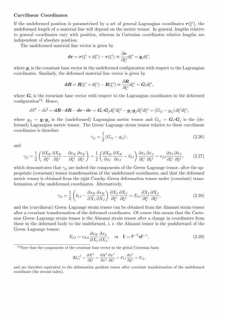
Curvilinear Coordinates

If the undeformed position is parametrised by a set of general Lagrangian coordinates r(ξi), theundeformed length of a material line will depend on the metric tensor. In general, lengths relativeto general coordinates vary with position, whereas in Cartesian coordinates relative lengths areindependent of absolute position.

The undeformed material line vector is given by

dr = r(ξi + dξi)− r(ξi) ≈ ∂r

∂ξidξi = gidξ

i,

where gi is the covariant base vector in the undeformed configuration with respect to the Lagrangiancoordinates. Similarly, the deformed material line vector is given by

dR = R(ξi + dξi)−R(ξi) ≈ ∂R

∂ξidξi = Gidξ

i,

where Gi is the covariant base vector with respect to the Lagrangian coordinates in the deformedconfiguration14. Hence,

dS2 − ds2 = dR · dR− dr · dr = Gi·Gjdξidξj − gi·gjdξ

idξj = (Gij − gij) dξidξj,

where gij = gi·gj is the (undeformed) Lagrangian metric tensor and Gij = Gi·Gj is the (de-formed) Lagrangian metric tensor. The Green–Lagrange strain tensor relative to these curvilinearcoordinates is therefore

γij =1

2(Gij − gij) ; (2.26)

and

γij =1

2

�∂XK

∂ξi∂XK

∂ξj− ∂xK

∂ξi∂xK

∂ξj

�=

1

2

�∂XK

∂xI

∂XK

∂xJ− δIJ

�∂xI

∂ξi∂xJ

∂ξj= eIJ

∂xI

∂ξi∂xJ

∂ξj, (2.27)

which demonstrates that γij are indeed the components of the Green–Lagrange tensor, after the ap-propriate (covariant) tensor transformation of the undeformed coordinates; and that the deformedmetric tensor is obtained from the right Cauchy–Green deformation tensor under (covariant) trans-formation of the undeformed coordinates. Alternatively,

γij =1

2

�δIJ − ∂xK

∂XI

∂xK

∂XJ

�∂XI

∂ξi∂XJ

∂ξj= EIJ

∂XI

∂ξi∂XJ

∂ξj, (2.28)

and the (curvilinear) Green–Lagrange strain tensor can be obtained from the Almansi strain tensorafter a covariant transformation of the deformed coordinates. Of course this means that the Carte-sian Green–Lagrange strain tensor is the Almansi strain tensor after a change in coordinates fromthose in the deformed body to the undeformed, i. e. the Almansi tensor is the pushforward of theGreen–Lagrange tensor:

EIJ = eKL∂xK

∂XI

∂xL

∂XJ, or E = F−T eF−1. (2.29)

14Note that the components of the covariant base vector in the global Cartesian basis

[Gj ]I=

∂XI

∂ξj=

∂XI

∂xJ

∂xJ

∂ξj= FIJ

∂xJ

∂ξj= FIj ,

and are therefore equivalent to the deformation gradient tensor after covariant transformation of the undeformedcoordinate (the second index).

The definition of F means that equation (1.30) defines the pushforward for covariant and contravari-ant tensors. Comparison with that equation reveals that E should be denoted E♭ to avoid mistakeswhen working in general coordinates.

The fact that all these tensors are equivalent should be no surprise — they all represent thesame physical measure: half the difference between the change in square lengths of material lineelements.

Relationship between Cartesian and curvilinear formulations

It seems to be most common in the literature to work in terms of the tensors F, c and C (or b andB) because it is more compact; but the meaning can be obscured. For example, consider a vectorfield that is convected with the motion of the continuum so that it obeys the same transformationrules as line elements, see also §5.2.4. If the vector field in the undeformed configuration is givenby a then by analogy with equation 2.19, the vector field in the deformed configuration, A, is givenby

AI = FIJaJ , (in global Cartesian components) or A = Fa.

A natural question is how to represent this in general curvilinear coordinates using the establishedmetric tensors. If we are completely explicit about the bases in our tensor formulation then itfollows that

F = FIJeI ⊗ eJ =∂XI

∂xJ

eI ⊗ eJ =∂XI

∂ξk∂ξk

∂xJ

eI ⊗ eJ =

�∂XI

∂ξkeI

�⊗�∂ξk

∂xJ

eJ

�

⇒ F = Gk ⊗ gk and hence F−1 = gk ⊗Gk,

which reveals the desired connection between the two formulations.Returning to the transformation of our vector field we can write

AiGi = F(aigi) ⇒ AiGj·Gi = Gj

·�Gk ⊗ gk

�·gia

i ⇒ Aiδji = δjkδki a

i ⇒ Aj = aj ,

and we might have expected. The result indicates that a vector field convected with continuum lineelements keeps identical values of its components, provided that covariant base vectors deform withthe motion of the continuum, i. e. if a = aigi, then A = aiGi.

If we have a vector field m, in the undeformed configuration, with different transformationproperties, e. g. the deformed configuration is given by M = F−Tm, then

M iGi = F−T (mi gi) ⇒ M iGj

·Gi = Gj·�Gk ⊗ gk

�·gi mi ⇒ M j = Gjkmk,

a different type of transformation.

2.4.1 The connection between deformation and displacement

From equation (2.5), the deformed position can be written as the vector sum of the undeformedposition and the displacement

R = r + u,

which means that

dR ≈ ∂(r + u)

∂ξidξi = (r,i + u,i) dξ

i = gi dξi + u,i dξ

i = dr + u,i dξi. (2.30)

The first term in equation (2.30) is the undeformed line element and so represents a rigid-bodytranslation; the second term contains all the information about the strain and rotation.

The covariant base vectors in the deformed configuration are

Gi = R,i = gi + u,i,

so the Green–Lagrange strain tensor becomes

γij =1

2

�Gi·Gj − gi·gj

�=

1

2

�(gi + u,i) ·

�gj + u,j

�− gij

�=

1

2

�gi·u,j + u,i·gj + u,i·u,j

�.

In order to simplify the scalar products, we write the displacement using the undeformed basevectors

u = uj gj, ⇒ u,i = uk|i gk,

where | represents the covariant derivative in the Lagrangian viewpoint with respect to Lagrangiancoordinates, i.e. using the metric tensor gij . Then the strain tensor becomes

γij =1

2

�gi·g

kuk|j + uk|igk·gj + uk|igk

·glul|j�=

1

2

�δki uk|j + uk|iδkj + uk|iul|jgkl

�

and so

γij =1

2

�ui|j + uj |i + uk|i uk|j

�.

The quantity with components ui|j is known as the displacement gradient tensor and can also bewritten ∇

r⊗ u. In our global Cartesian coordinate system, the Green–Lagrange strain tensor has

the form

eIJ =1

2[uI,J + uJ,I + uK,I uK,J ] , (2.31)

which is often seen in textbooks.

2.4.2 Interpretation of the deformed metric (right Cauchy–Green de-

formation) tensor Gij

We can scale the infinitesimal increments in the general coordinates so that dξi = ni dǫ, where ni

represents the direction of the increment and is chosen so that the vector n = ni gi has unit length,

n · n = ni gi·njgj = nigijn

j = 1.

The undeformed and deformed line elements are then functions of the direction n

dr(n) = ginidǫ and dR(n) = Gin

idǫ.

We define the stretch in the direction n to be the ratio of the length of the deformed line elementto the undeformed line element:

λ(n) =|dR(n)||dr(n)| =

pniGijnjdǫpnigijnjdǫ

=pniGijnj =

√nIcIJnJ , (2.32)

where the last equality is obtained on transformation from the general coordinates to the globalCartesian coordinates. Note that the stretch is invariant and is well-defined because we have alreadyestablished that nIcIJnJ > 0 for all non-zero n.

If we define n(i) to be a unit vector in the ξi direction, then n(i)i = 1/

√gii (not summed) n

(i)j = 0,

j 6= i, soλ(n(i)) =

pGii/gii (not summed),

which means that the diagonal entries of the deformed metric tensor are proportional to the squaresof the stretch in the coordinate directions. If the undeformed coordinates are Cartesian coordinates,for which gii = 1 (not summed), then the diagonal entries of the deformed metric tensor are exactlythe squares of the stretches in coordinate directions.

We now consider two distinct line elements in the undeformed configuration

dr = nigi dǫ and dq = migi dǫ,

where nigi and migi are both unit vectors. The corresponding line elements in the deformedconfiguration are

dR = niGi dǫ and dQ = miGi dǫ.

The dot product of the two deformed line elements is

niGijmj(dǫ)2 = |dR||dQ| cosΘ =

pniGijnj dǫ

pmiGijmj dǫ cosΘ,

where Θ is the angle between the two deformed line elements. Thus,

cosΘ =niGijm

j

pniGijnj

pmiGijmj

; (2.33)

and if θ is the angle between the two undeformed line elements

cos θ = nigijmj .

Thus, the information about change in length and relative rotation of two line elements is entirelycontained within the deformed metric tensor.

Example 2.4. Rigid body motionIf the body undergoes a rigid-body motion show that every component of the Green–Lagrangestrain tensor is zero.

Solution 2.4. In a rigid-body motion the line elements do not change lengths and the anglesbetween any two line elements remain the same. Hence, for any unit vectors n and m in theundeformed configuration

λ(n) = niGijnj = 1, λ(m) = miGijm

j = 1, (2.34a)

and cosΘ = cos θ, which means that

niGijmj = nigijmj

pniGijnj

pmiGijmj . (2.34b)

Using equation (2.34a) in equation (2.34b), we obtain the condition

niGijmj = nigijm

j ⇒ ni (Gij − gij)mj = 0,

which must be true for all possible unit vectors n and m and so by picking the nine differentcombinations on non-zero components, it follows that Gij − gij = 0 for all i, j. Hence, everycomponent of the Green–Lagrange strain tensor is zero.

2.4.3 Strain Invariants and Principal Stretches

At any point, the direction of maximum stretch is given by

maxn

λ(n) subject to the constraint |n| = 1,

which can be solved by the method of Lagrange multipliers. We seek the stationary points of thefunction

L(n, µ) = λ2(n)− µ�gijn

inj − 1= ninjGij − µ

�gijn

jni − 1,

where µ is an unknown Lagrange multiplier and ni are the components of the unit vector in thebasis gi. The condition ∂L/∂µ = 0 recovers the constraint and the three other partial derivativeconditions give

∂L

∂ni= 0 ⇒ Gijn

j − µgijnj = (Gij − µgij)n

j = 0. (2.35)

Thus, the maximum (or minimum) stretch is given by non-trivial solutions of the equation (2.35),which is an equation that defines the eigenvalues and eigenvectors of the deformed metric tensor.

The deformed metric tensor has real components and is symmetric which means that it has realeigenvalues and mutually orthogonal eigenvectors15. The eigenvectors v are non-trivial solutions ofthe equation

G(v) = µv or Gijvj = µgijv

j = µvi, etc, (2.36)

where G represents the deformed metric tensor as a linear map and the scalars µ are the associatedeigenvalues. Note that because the eigenvalues are scalars they do not depend on the coordinatesystem, but, of course, the components of the eigenvectors are coordinate-system dependent. Theeigenvalues (or in fact any functions of the eigenvalues) are, therefore, scalar invariants of thedeformed metric tensor.

Equation (2.36) only has non-trivial solutions if

det(Gij − µ gij) = 0.

and expansion of the determinant gives a cubic equation for µ, so there are three real eigenvaluesand, hence, three distinct invariants. The invariants are not unique, but those most commonly usedin the literature follow from the expansion of the determinant of the mixed deformed metric tensorin which the index is raised by multiplication with undeformed covariant metric tensor16 whichmeans that the undeformed metric tensor becomes the Kronecker delta:

|gikGkj − µδij| = −µ3 + I1µ2 − I2µ+ I3. (2.37)

Expanding the determinant using the alternating symbol gives

eijk(G1i − µ δ1i )(G

2j − µ δ2j )(G

3k − µ δ3k)

= eijk�G1

iG2jG

3k − µ

�δ1iG

2jG

3k + δ2jG

1iG

3k + δ3kG

1iG

2j

�+ µ2

�δ1i δ

2jG

3k + δ1i δ

3kG

2j + δ2j δ

3kG

1i

�− µ3δ1i δ

2j δ

3k

�,

15This is a fundamental result in linear algebra is easily proved for distinct eigenvalues by considering the appro-priate dot products between different eigenvectors and also between an eigenvector and its complex conjugate. Forrepeated eigenvalues the proof proceeds by induction on subspaces of successively smaller dimension.

16In other words we are defining Gij = gikGkj , which is a slight abuse of notation: if we worked solely in the

deformed metric then we would define Gij = GikGjk = δij. The fact that our definition of Gi

j 6= δij is why we canreuse the notation without ambiguity, but it has the potential to be confusing.

and on comparison with equation (2.37) we obtain

I1 = G11 +G2

2 +G33 = Gi

i = trace(G), (2.38a)

I2 = G22G

33 −G2

3G32 +G1

1G33 −G1

3G31 +G1

1G22 −G1

2G21,

=1

2

�Gi

iGjj −Gi

jGji

�=

1

2

�(trace(G))2 − trace(G2)

�. (2.38b)

I3 = eijkG1iG

2jG

3k = |Gi

j| = |gikGkj| = |gik||Gkj| = G/g, (2.38c)

where G = |Gij| is the determinant of the deformed covariant metric tensor and g = |gij| is thedeterminant of the undeformed covariant metric tensor.

The use of invariants will be an essential part of constitutive modelling, because the behaviourof a material should not depend on the coordinate system.

The mutual orthogonality of the eigenvectors means that they form a basis of the Euclidean spaceand if we choose the eigenvectors to have unit length we can write the eigenbasis as v�I = v

�I . Thecircumflexes on the indices are used to indicate the eigenbasis rather than the standard Cartesianbasis. The components of the deformed metric tensor in the eigenbasis are given by

G�I �J = v�I·G(v �J) = v�I·µ( �J)v �J = µ( �J)v�I·v �J ( bJ not summed),

where µ( �J) is the eigenvalue associated with the eigenvector v �J . Thus the components of thedeformed metric tensor in the eigenbasis form a diagonal matrix with the eigenvalues as diagonalentries

G�I �J =

(µ(�I)

bI = bJ,0 bI 6= bJ,

= µ(�I) δ�I �J (not summed).

or writing the components in the eigenbasis in matrix form

G =

µ1 0 00 µ2 00 0 µ3

, (2.39)

or

G =3X

�I=1

µ(�I)v�I ⊗ v�I .

These eigenvalues are related to the stretch because if we decompose a unit vector into theeigenbasis, n = n�Iv�I , then from equation (2.32)

λ(n) =p

n�IG�I �Jn �J =

vuut3X

�I=1

n�Iµ(�I)n�I ,

and so the stretches in the direction of the eigenvectors are the square-roots17 of the associatedeigenvalues

λ(v�I) ≡ λ(�I) =p

µ(�I). (2.40)

The three quantities λ(�I) are called the principal stretches and the associated eigenvectors are theprincipal axes of stretch.

17We could have anticipated this result because the metric tensor was formed by taking the square of the lengthsof line elements.

These results motivate the definition of another symmetric tensor in which the eigenvectorsremain the same, but the eigenvalues coincide exactly with the stretches

U =

3X

�I=1

λ(�I)v�I ⊗ v�I =

3X

�I=1

pµ(�I)v�I ⊗ v�I =

√G.

The deformed metric tensor can be written as the product of the deformation gradient tensor andits transpose, so in matrix form in Cartesian coordinates (although the coordinates don’t matterbecause the quantities are all tensors)

c = FTF = U2.

Recall that the matrix c is the Cauchy–Green deformation tensor, which is the deformed metrictensor when the Lagrangian and Eulerian coordinates are both Cartesian. We define

R = FU−1 ⇒ F = RU,

and note that because U is symmetric U−1 = U−T and so

RTR = (FU−1)T (FU−1) = U−TFTFU−1 = U−1U2U−1 = I,

so R is orthogonal. Hence, F can be written as the product of an orthogonal transformation (rota-tion) and U which is known as the (right) stretch tensor18. The interpretation is that, in additionto rigid-body translation, any deformation consists (locally) of a rotation and three mutually or-thogonal stretches — the principal stretches, which are the square-roots of the eigenvalues of thedeformed metric tensor.

2.4.4 Alternative measures of strain

The strain is zero whenever the principal stretches are all of unit length, so in the eigenbasisrepresentation the matrix of components of the right stretch tensor is U = I. However, the eigenbasisis orthonormal and therefore any other Cartesian basis is obtained via orthogonal transformationso that the matrix representation of the stretch tensor becomes,

U = QUQT = QIQT = QQT = I.

Hence, if the strain is zero then U = I when the stretch tensor is represented in any orthonormalcoordinate system. Transforming to a general coordinate system would give Uij = gij in the zerostrain case, where gij is the undeformed metric tensor.

We can define general strain measures using tensor functions of the right stretch tensor F(U).In the eigenbasis U is diagonal and we define F(U) by

F(U) =3X

�I=1

f�λ(�I)

�v�I ⊗ v�I ,

where f(x) is any monotonically increasing function such that f(1) = 0 and f′

(1) = 1. Themonotonicity ensures that an increase in stretch leads to an increase in strain; the condition f(1) = 0

18This result is often called the polar decomposition. It is unique and the orthogonal transformation does notinvolve any reflection because detR > 0, which follows from detU > 0 and detF > 0.

means that when there is no stretch there is no strain; and the condition f′

(1) = 1 is a normalisationto ensure that all strain measures are the same when linearised and consistent with the theory ofsmall deformations. Admissible functions include

f(x) =1

m(xm − 1) (m 6= 0) and ln x (m = 0).

In orthonormal coordinate systems, we can then write the corresponding strain measures as

1

m(Um − I) (m 6= 0) and lnU (m = 0).

The case m = 2 corresponds to the Green–Lagrange strain tensor; the case m = −2 is theAlmansi strain tensor; the case m = 1 is called the Biot strain tensor and the case m = 0 is calledthe Hencky or incremental strain tensor.

Note that it is only the Green–Lagrange and Almansi strain tensors that can be formed withoutprior knowledge of the eigenvectors, so these are most commonly used in practice.

2.4.5 Deformation of surface and volume elements

Having characterised the deformation of material line elements, we will also find it useful to con-sider the deformation of material surfaces and volumes. This will be particularly important whendeveloping continuum conservation, or balance, laws.

Volume elements

We already know from equation (1.46) that a volume element in the undeformed configuration isgiven by dV0 =

√g dξ1dξ2dξ3. The corresponding volume element in the deformed configuration is

given by dVt =√G dξ1dξ2dξ3. Hence, the relationship between the two volume elements is

dVt =p

G/g dV0. (2.41a)

From equation (2.19)

FIJ =∂XI

∂xJ=

∂XI

∂ξi∂ξi

∂xJ,

which means that J = det F =√G/

√g from equation (1.44). Thus we can also write the change in

volume using the determinant of the deformation gradient tensor

dVt = det F dV0 = J dV0. (2.41b)

Surface elements

If we now consider a vector surface element given by da = n da in the undeformed configuration,where da is the area and n is a unit normal to the surface. We can form a volume element bytaking the dot product of the vector surface element and a line element dr, so

dV0 = dv = dr·da = nI drI da.

From equation (2.41b) the corresponding deformed volume element is

dVt = dV = JnI drI da = NI dRI dA = dR·dA,

where dA = N dA is the deformed vector surface element. From equation (2.19) dRI = FIJ drJ ,so

JnI drI da = NIFIJ drJ dA, ⇒ JnJ da = NIFIJ dA

⇒ dAI = NI dA = JnJF−1JI da = JF−1

JI daJ ⇒ N dA = JF−Tnda, (2.42)

a result known as Nanson’s relation.Converting to general tensor notation, we decompose the deformed area vector dA = N dA

into the deformed contravariant basis in the Eulerian coordinates χi, to obtain

dAi = dAI∂XI

∂χi= J

∂xJ

∂XIdaJ

∂XI

∂χi= J

∂xJ

∂χidaJ = J

∂ξj

∂χi

∂xJ

∂ξjdaJ = J

∂ξj

∂χidaj , (2.43)

where the undeformed area vector has been decomposed into the undeformed contravariant basisin Lagrangian coordinates, da = daig

i. Thus, the transformation is similar to the usual covarianttransformation between Eulerian and Lagrangian coordinate systems, but with an additional scalingby J to compensate for the change in area.

2.4.6 Special classes of deformation

If the deformation gradient tensor, FIJ , is a function only of time (does not vary with position)then the deformation is said to be homogeneous. In this case, the equation (2.19)

dRI(t) = FIJ(t) drJ ,

and integrating between two material points, at positions a and b in the undeformed configuration,gives

AI(t)− BI(t) = FIJ(t) (aI − bI) , (2.44)

whereA andB are the corresponding positions of the material points in the deformed configuration.Equation (2.44) demonstrates that straight lines are carried to straight lines in a homogeneousdeformation. Furthermore, any homogeneous deformation can be written in the form

XI = AI(t) + FIJ(t) xJ .

• Pure strain is such that the principal axes of strain are unchanged, which means that therotation tensor in the polar decomposition is the identity R = I.

• Rigid-body deformations are such that the distance between every pair of points remainsunchanged and we saw in Example 2.4 that the strain is zero in such cases. We can also showthat in this case the invariants are I1 = I2 = 3 and I3 = 1.

• Isochoric deformation is such that the volume does not change, which means that J =√I3 = 1.

• Uniform dilation is a homogeneous deformation in which FIJ = λδIJ , which means that allthe principal stretches are λ. In other words, the material is stretched equally in all directions.

• Uniaxial strain is a homogeneous deformation in which one of the principal stretches is λand the other two are 1, i.e. the material is stretched (and therefore strained) in only onedirection.

• Simple shear is a homogeneous deformation in which all diagonal elements of F are 1 andone off-diagonal element is nonzero.

2.4.7 Strain compatibility conditions

The strain tensors are symmetric tensors which means that they have six independent components,but they are determined from the displacement vector which has only three independent compo-nents. If we interpret the six equations (2.31) as a set of differential equations for the displacement,assuming that we are given the strain components, then we have an overdetermined system. Itfollows that there must be additional constraints satisfied by the components of a strain tensor toensure that a meaningful displacement field can be recovered.

One approach to determine these conditions is to eliminate the displacement components fromthe equations (2.31) by partial differentiation and elimination, which is tedious particularly incurvilinear coordinates. A more sophisticated approach is to invoke a theorem due to Riemann thatthe Riemann–Christoffel tensor formed from a symmetric tensor gij should be zero if the tensor isa metric tensor of Euclidean space. The Riemann–Christoffel tensor is motivated by consideringsecond covariant derivatives of vectors

vi|jr = (vi|j)|r = (vi|j),r − Γkir(vk|j)− Γk

jr(vi|k),

see Example Sheet 1, q. 10. Writing out the covariant derivatives gives

vi|jr = vi,jr − Γlij,rvl − Γl

ijvl,r − Γkirvk,j + Γk

irΓlkjvl − Γk

jrvi,k + ΓkjrΓ

likvl. (2.45a)

Interchanging r and j gives

vi|rj = vi,rj − Γlir,jvl − Γl

irvl,j − Γkijvk,r + Γk

ijΓlkrvl − Γk

rjvi,k + ΓkrjΓ

likvl, (2.45b)

and subtracting equation (2.45b) from equation (2.45a) gives

vi|jr − vi|rj =�Γlir,j − Γl

ij,r + ΓkirΓ

lkj − Γk

ijΓlkr

�vl ≡ Rl

.ijr vl,

after using the symmetry properties of the Christoffel symbol and the partial derivative. Thequantities on the left are the components of the type (0,3) tensors and vl are the components ofa type (0,1) tensor, which means that Rl

.ijr is a type (1,3) tensor called the Riemann–Christoffeltensor. Thus if Rl

.ijr = 0, then covariant derivatives commute. The tensor is a measure of thecurvature of space and in Cartesians coordinate in an Eulerian space the Christoffel symbols are allzero, which means that Rl

.ijr = 0 in any coordinate system in our Eulerian space.A physical interpretation for compatibility conditions is that a deformed body must “fit together”

so that a continuous region of space is filled. Thus, the tensor Gij associated with the deformedmaterial points must be a metric tensor of our Euclidean space and the required conditions are thatthe Riemann–Christoffel symbol associated with Gij must be zero. We can use the relationship

γij =1

2(Gij − gij) ⇒ Gij = 2γij + gij ,

to determine explicit equations for the conditions on the components of the Green–Lagrange straintensor γij, but these are somewhat cumbersome.

2.5 Deformation Rates

In many materials, particularly fluids, it is the rate of deformation, rather than the deformationitself that is of most importance. For example if we take a glass of water at rest and shake it

(gently) then wait, the water will come to rest and look as it did before we shook it. However,the configuration of the material points will almost certainly have changed. Thus, the fluid willhave deformed significantly, but this does not affect its behaviour. The obvious “rates” are materialtime derivatives of objects that quantify the deformation. The general approach when computingmaterial derivatives of complicated objects is to work in the undeformed configuration, by using (ortransforming to) Lagrangian coordinates, in which case the time-derivative is equal to the partialderivative and the coordinates are fixed in time. We shall use such an approach throughout theremainder of this chapter.

A measure of the rate of deformation of material lines is given by

D

Dt

�|dR|2

�=

∂

∂t

����r

�|dR|2

�=

∂

∂t

����ξ

�Gij dξ

idξj�=

∂Gi

∂t

����ξ

·Gj +Gi·∂Gj

∂t

����ξ

!dξidξj,

because the Lagrangian coordinates ξi are fixed on material line and are independent of time. Thefact that time and the Lagrangian coordinates are independent means that

DGi

Dt=

∂Gi

∂t

����ξ

=∂2R

∂t ∂ξi=

∂

∂ξiDR

Dt= v,i =

�VkG

k�,i= Vk||iGk, (2.46)

where || indicates covariant differentiation in the Lagrangian deformed basis with covariant basevectors Gi and contravariant base vectors Gi. Thus,

D

Dt

�|dR|2

�=

�Vk||iGk

·Gj + Vk||jGi·Gk�dξidξj = (Vi||j + Vj||i) dξidξj.

Now because the undeformed line element dr has constant length, we can write

D

Dt

�|dR|2

�=

D

Dt

�|dR|2 − |dr|2

�=

D

Dt

�2γij dξ

idξj�= 2γij dξ

idξj,

where

γij =DγijDt

=1

2(Vi||j + Vj||i) , (2.47)

is the (Lagrangian) rate of deformation tensor and is the material derivative of the Green–Lagrangestrain tensor.

Alternatively, we could have decomposed the velocity into the (curvilinear) Eulerian coordinatesχj , in which case

∂v

∂ξi=

∂χl

∂ξi∂V

∂χl=

∂χl

∂ξiVk||lGk,

and thenD

Dt

�|dR|2

�=

∂χl

∂ξiVk||lGk

·Gj +∂χl

∂ξjVk||lGk

·Gi

!dξidξj,

=

∂χl

∂ξiVk||l

∂χk

∂ξmGm

·Gj +∂χl

∂ξjVk||l

∂χk

∂ξmGm

·Gi

!dξidξj,

= (Vk||l + Vl||k)∂χk

∂ξi∂χl

∂ξjdξidξj = 2Dk l dχ

kdχl, (2.48)

where

Di j =1

2

�Vi||j + Vj ||i

�,

is the Eulerian rate of deformation tensor in components in the Eulerian curvilinear basis.At a given time, we can recover the Lagrangian rate of deformation tensor from the Eulerian by

simply applying the appropriate covariant transformation; γij is the pullback of D♭ and is thereforeequal to Dij componentwise.

However, an important point is that although the Lagrangian rate of deformation tensor is thematerial time-derivative of the (Green-Lagrange) strain tensor. The Eulerian rate of deformationtensor, in general, does not coincide with the spatial or material time-derivative of an Eulerianstrain tensor because the Eulerian coordinates themselves vary with time.

In the Eulerian representation (in Cartesian coordinates for convenience)

D

Dt

�|dR|2

�=

D

Dt(2EIJ dXIdXJ) = 2

DEIJ

DtdXI dXJ + 2EIJ

D(dXI)

DtdXJ + 2EIJdXI

D(dXJ)

Dt,

and the material time derivative of the Eulerian line element is not zero in general. In fact, makinguse of Lagrangian coordinates,

D(dXI)

Dt=

D

Dt

�∂XI

∂xJdxJ

�=

∂

∂xJ

�DXI

Dt

�dxJ ,

because the material derivative and the Lagrangian coordinates are independent. By definition, thematerial derivative of the Eulerian position is the Eulerian velocity, which in Cartesian coordinatesis given by V = VIeI , so

D(dXI)

Dt=

∂VI

∂xJdxJ =

∂VI

∂XK

∂XK

∂xJdxJ =

∂VI

∂XKdXK .

Thus,D

Dt(2EIJ dXIdXJ) = 2

�DEIJ

Dt+ EIKVK,J + EKJVK,I

�dXI dXJ

= 2Di j dχi dχj = 2DIJ dXIdXJ ,

after transformation to Cartesian coordinates. The equation is valid for arbitrary dXI and dXJ , so

EIJ = DIJ −EIKVK,J −EKJVK,I . (2.49)

Hence, if the Eulerian rate of deformation DIJ is zero, but the material is strained EIJ 6= 0, anEulerian observer will perceive a rate of strain of

EIJ = −EIKVK,J −EKJVK,I,

which is a consequence of the movement of the material lines in the fixed Eulerian coordinatesystem.

2.5.1 Rates of stretch, spin & vorticity

The Eulerian velocity gradient tensor is given by

Li j = Vi||j, or LIJ =∂VI

∂XJ,

which means that the (Eulerian) deformation rate tensor is the symmetric part of the (Eulerian)velocity gradient tensor,

Di j =1

2

�Li j + Lj i

�. (2.50)

The antisymmetric part of the (Eulerian) velocity gradient tensor is called the spin tensor

Wi j =1

2

�Li j − Lj i

�,

and so by constructionLi j = Di j +Wi j.

The vorticity vector is a vector associated with the spin tensor and is defined by

ωk = ǫk i jWj i =1

2ǫk i j

�Vj ||i − Vi||j

�= ǫk i jVj||i,

where ǫi j k is the Levi-Civita symbol in the Eulerian curvilinear coordinates χi, which means that

ω = curlRV ,

in the Eulerian framework.We can now use the same arguments as in §2.4.2 to demonstrate that the the diagonal entries

DII (not summed) are the instantaneous rates of stretch along Cartesian coordinate axes and thatthe off-diagonal entries represent the instantaneous rate of change in angle between two coordinatelines, or one-half the rate of shearing.

In addition, equation (2.46) expresses the material derivative of our Lagrangian base vectors,i.e. how lines tangent to the Lagrangian coordinates evolve with the deformation. Expressing theequation (2.46) in Cartesian coordinates gives

DGi

Dt= Vk||iGi ⇒ DFIi

DteI = Vk||i

∂ξk

∂XIeI ,

⇒ DFIi

Dt= vk||i

∂ξk

∂XI= VI ||i = VI,K

∂XK

∂ξi= VI,KFKi ⇒ DFIJ

Dt= VI,KFKJ , (2.51)

which demonstrates that the material derivative of the deformation gradient tensor is simply thevelocity gradient tensor composed with the deformation gradient. A physical interpretation is thatit is gradients (differences) in velocity that lead to changes in material deformation, which explainsthe above identification of the rate of deformation with the velocity gradient.

We next introduce the relative deformation gradient tensor, in which we measure the deformationfrom the initial state to a time τ and then the deformation from time τ to a subsequent time t.Then

FIJ(t) =∂XI(t)

∂xJ=

∂XI(t)

∂XK(τ)

∂XK(τ)

∂xJ= FIK(t, τ)FKJ(τ),

where FIK(t, τ) is called the relative deformation gradient tensor. The deformation gradient at thefixed time τ is independent of t so that

DFIJ

Dt=

DFIK(t, τ)

DtFKJ(τ), (2.52)

and taking the limit τ → t of equation (2.52) and comparing to equation (2.51) we see that

DFIK(t, τ)

Dt

�����τ=t

= VI,K, or written as matricesDF(t, τ)

Dt

�����τ=t

= L,

and the instantaneous relative deformation tensor is given by the Eulerian velocity gradient tensor.We can now use the polar decomposition to write

DF

Dt=

D(RU)

Dt

�����τ=t

= L = D+W

⇒ R���τ=t

DU

Dt

�����τ=t

+DR

Dt

�����τ=t

U���τ=t

= D+W.

Now the relative rotation R and stretch U tensors both tend to the identity as τ → t and there isdifference between the state at τ and t. Thus,

DU

Dt

�����τ=t

+DR

Dt

�����τ=t

= D +W.

The (right) stretch tensor U is symmetric which means that

DU

Dt

�����τ=t

= D andDR

Dt

�����τ=t

= W,

with the interpretation that the instantaneous material rate of change of the stretch tensor, i.e. therate of stretch is given by the Eulerian deformation rate tensor; and the instantaneous material rateof rotation is given by the spin tensor.

2.5.2 Material derivative of volume and area elements

A volume element in the current (deformed) position is given by

dVt =√Gdξ1dξ2dξ3,

so the material derivative of the volume gives the dilation rate

D dVt

Dt=

D√G

Dtdξ1dξ2dξ2.

We use a similar approach to that in the proof of the divergence theorem to determine

D√G

Dt=

1

2√G

DG

Dt=

1

2√G

∂G

∂Gij

DGij

Dt.

From comparison with equation (1.56) we have

∂G

∂Gij

= GGij, (2.53)

and using equation (2.46)

DGij

Dt=

DGi

Dt·Gj +

DGj

Dt·Gi = Vi||j + Vj ||i.

Hence,

D√G

Dt=

1

2√GGGij (Vi||j + Vj||i) =

1

2

√G�V j ||j + V i||i

�=

√GV i||i =

√GV i||i, (2.54)

after change of coordinates from Lagrangian to Eulerian. In other words, the rate of change of avolume element is given by

D dVt

Dt= V i||i

√G dξ1dξ2dξ3 = V i||i dVt,

and the relative volume change, or dilation, is

1

dVt

DdVt

Dt= V i||i = div

RV , (2.55)

the divergence of the Eulerian velocity field.The material derivative of an area element can be obtained by using the equation (2.43) to map

the area element back into the Lagrangian coordinates

D dAi

Dt=

D

Dt

�J∂ξj

∂χidaj

�=

�DJ

Dt

∂ξj

∂χi+ J

D

Dt

�∂ξj

∂χi

��daj .

= V k||kJ∂ξj

∂χidaj − V l||iJ

∂ξj

∂χldaj = V k||kdAi − V l||idAl. (2.56)

The first term is obtained on using the result (2.54) divided by√g because J =

pG/g and

√g is

constant under material differentiation. The second term uses the result that

D

Dt

�∂ξj

∂χi

�= −V l||i

∂ξj

∂χl, (2.57)

which has a non-trivial derivation in curvilinear coordinates19 because we need to be careful aboutwhat is being held fixed when computing all the derivatives. Firstly, we note that

D

Dt

∂χi

∂ξj

!=

D

Dt

�χi,j

�=

∂χi,j

∂t

�����r

+ V l∂χi

,j

∂χl

�����t

+ V l Γi

lm χm,j , (2.58)

19The derivation in Cartesians is even simpler because the complexity of covariant differentiation is finessed,

D

Dt

�∂XJ

∂xI

�=

∂

∂xI

DXJ

Dt=

∂VJ

∂xI

=∂VJ

∂XK

∂XK

∂xI

= VJ,K

∂XK

∂xI

, orDF

Dt= LF;

and thenD

Dt

�∂XJ

∂xI

∂xI

∂XL

�=

D

Dt

�∂XJ

∂xI

�∂xI

∂XL

+∂XJ

∂xI

D

Dt

�∂xI

∂XL

�=

D

Dt(δJL) = 0,

⇒ ∂XJ

∂xI

D

Dt

�∂xI

∂XL

�= − D

Dt

�∂XJ

∂xI

�∂xI

∂XL

= −VJ,K

∂XK

∂xI

∂xI

∂XL

= −VJ,KδKL = −VJ,L

⇒ D

Dt

�∂xK

∂XL

�= −VJ,L

∂xK

∂XJ

, orDF−1

Dt= −F−1L.

because although the quantity χi,j is a two-point tensor, the Lagrangian component is unaffected

by material differentiation. Thus, the material derivative of χi,j is the same as for a contravariant

vector component. The velocity is given by

V =∂R(χi(r, t))

∂t

�����r

=∂R

∂χi

∂χi

∂t

�����r

=∂χi

∂t

�����r

Gi,

which means that the components of the Eulerian velocity vector in the basis Gi are given by

V i = ∂χi

∂t|r . Thus, equation (2.58) can be rewritten as

D

Dt

∂χi

∂ξj

!=

∂χi,j

∂t

�����r

+∂χl

∂t

�����r

∂χi,j

∂χl

�����t

+ V l Γi

l m χm,j =

dχi,j

dt+ V l Γ

i

l m χm,j , (2.59)

where d/dt is the total derivative with respect to time and, in the Eulerian framework, χi,j is a

function of χi(t) and t. Now,

dχi,j

dt=

d

dt

∂χi(ξj, t)

∂ξj

!=

∂

∂t

∂χi

∂ξj

!=

∂

∂ξj

∂χi

∂t

!=

∂V i

∂ξj,

because the Lagrangian coordinates are not functions of time and so the partial time derivative isequal to the material derivative. Equation (2.59) can therefore be written as

D

Dt

∂χi

∂ξj

!= V i

,j + V l Γi

lm χm,j =

hV i,m + V l Γ

i

lm

iχm,j = V i||m χm

,j ,

after using the chain rule. The right-hand side has the appropriate two-point tensor transformationproperties.

In order to derive equation (2.57), we use the fact that

D

Dt

∂ξk

∂χi

∂χi

∂ξj

!=

D

Dt

�δkj�= 0,

to writeD

Dt

�∂ξk

∂χi

�∂χi

∂ξj+

∂ξk

∂χi

D

Dt

∂χi

∂ξj

!= 0

⇒ D

Dt

�∂ξk

∂χi

�∂χi

∂ξj= −∂ξk

∂χi

D

Dt

∂χi

∂ξj

!= −∂ξk

∂χiV i||m

∂χm

∂ξj

and multiplying both sides by ∂ξj/∂χl gives

⇒ D

Dt

�∂ξk

∂χl

�= −∂ξk

∂χiV i||l,

as required.We can interpret the result for the transformation of the area element as follows

D dAi

Dt= V k||k dAi − V l||i dAl,

Material Derivative = Volume Expansion − Expansion normalof Area to Area Element.

2.6 The Reynolds Transport Theorem

The Reynolds transport theorem concerns the time derivative of integrals over material volumes(although it can be generalised to arbitrary moving volumes by considering a new set of coordinatesthat move with the volume in question rather than with the fluid)

∂I(t)∂t

=dI(t)dt

=d

dt

Z

Ωt

φ dVt.

Integrating φ(R, t) over space means that I is a function only of t so the total derivative is equalto the partial derivative. Firstly we transform the material volume to the equivalent undeformedvolume

dIdt

=d

dt

Z

Ω0

φp

G/g√g dξ1dξ2dξ3 =

d

dt

Z

Ω0

φpG/g dV0,

and because the undeformed volume is fixed, we can take the time derivative under the integral sothat

dIdt

=

Z

Ω0

∂

∂t

�φpG/g

�dV0 =

Z

Ω0

∂φ

∂t

pG/g + φ

∂p

G/g

∂t

!dV0.

In the undeformed configuration we take the partial time derivative with r held constant, i.e. thematerial derivative D/Dt = ∂/∂t, and

dIdt

=

Z

Ω0

Dφ

Dt

sG

g+

φ√g

D√G

Dt

!dV0 =

Z

Ω0

�Dφ

Dt+ φ V i||i

�sG

gdV0 =

Z

Ωt

�Dφ

Dt+ φ V i||i

�dVt,

after using equation (2.54) and transforming back to the material volume. Thus, we can write

d

dt

Z

Ωt

φ dVt =

Z

Ωt

�Dφ

Dt+ φ∇

R·V

�dVt,

or expanding the material derivative

d

dt

Z

Ωt

φ dVt =

Z

Ωt

�∂φ

∂t+ V · ∇

Rφ+ φ∇

R·V

�dVt =

Z

Ωt

�∂φ

∂t+∇

R·(φV )

�dVt;

and using the divergence theorem

d

dt

Z

Ωt

φ dVt =

Z

Ωt

∂φ

∂tdVt +

Z

∂Ωt

φV ·N dSt,

which means that the time rate of change of a quantity within a material volume is the sum ofits rate of change obtained by treating the volume as fixed and the flux of the quantity across theboundaries (due to the movement of the boundaries).

In fact, the result is the multi-dimensional generalisation of the Leibnitz rule for differentiatingunder the integral sign when the limits are functions of the integration variable. Consider

∂I

∂t=

dI

dt=

∂

∂t

Z b(t)

a(t)

f(x, t) dx = limδt→0

R b(t+δt)

a(t+δt)f(x, t+ δt) dx−

R b(t)

a(t)f(x, t) dx

δt,

from the fundamental definition of the partial derivative. Splitting up the domain of integration forthe first integral gives

∂I

∂t= lim

δt→0

R a(t)

a(t+δt)f(x, t+ δt) dx+

R b(t)

a(t)f(x, t + δt) dx+

R b(t+δt)

b(t)f(x, t+ δt) dx−

R b(t)

a(t)f(x, t) dx

δt.

Now, assuming that all the limits exist we can write

∂I

∂t=

Z b(t)

a(t)

limδt→0

[f(x, t+ δt)− f(x, t)]

δtdx

+ limδ→0

1

δt

"Z a(t)

a(t+δt)

f(x, t+ δt) dx+

Z b(t+δt)

b(t)

f(x, t + δt) dx

#.

The first integral is simply the integral of ∂f/∂t and the others can be written using the mean valuetheorem as the product of the length of the integration interval and the function evaluated at somepoint within the interval, so

∂I

∂t=

Z b(t)

a(t)

∂f

∂tdx+ lim

δt→0

1

δt{[a(t)− a(t+ δt)]f(x, τa) + [b(t + δt)− b(t)]f(x, τb)} ,

where a(t) < τa < a(t + δt) and b(t) < τb < b(t + δt). Using Taylor’s theorem to expand the termsa(t + δt) and b(t + δt) we obtain

∂I

∂t=

Z b(t)

a(t)

∂f

∂tdx+ lim

δt→0{−a′(t)f(x, τa) + b′(t)f(x, τb)} =

Z b(t)

a(t)

∂f

∂tdx− a′(t)f(x, a) + b′(t)f(x, b),

because τa → a and τb → b as δt → 0, where the last two terms can be identified as the flux of fout of the moving domain.