energies

Article

Definition and Experimental Validation of aSimplified Model for a Microgrid Thermal Networkand its Integration into Energy Management Systems

Andrea Bonfiglio 1,*, Massimo Brignone 1, Federico Delfino 1, Alessandro Nilberto 2

and Renato Procopio 1

1 Department of Naval, Electrical, and ICT Engineering, University of Genova, I-16145 Genoa, Italy;massimo.brignone@gmail.com (M.B.); federico.delfino@unige.it (F.D.); renato.procopio@unige.it (R.P.)

2 Mechanical, Energy, Management and Transportation Engineering Department, University of Genova,I-16145 Genoa, Italy; a.nilberto@unige.it

* Correspondence: a.bonfiglio@unige.it; Tel.: +39-010-353-2730

Academic Editor: Brian AgnewReceived: 29 August 2016; Accepted: 2 November 2016; Published: 4 November 2016

Abstract: The present paper aims at defining a simplified but effective model of a thermal networkthat links the thermal power generation with the resulting temperature time profile in a heatedor refrigerated environment. For this purpose, an equivalent electric circuit is proposed togetherwith an experimental procedure to evaluate its input parameters. The paper also highlights thesimplicity of implementation of the proposed model into a microgrid Energy Management System.This allows the optimal operation of the thermal network to be achieved on the basis of availabledata (desired temperature profile) instead of a less realistic basis (such as the desired thermalpower profile). The validation of the proposed model is performed on the Savona Campus SmartPolygeneration Microgrid (SPM) with the following steps: (i) identification of the parameters involvedin the equivalent circuit (performed by minimizing the difference between the temperature profile,as calculated with the proposed model, and the measured one in a set of training days); (ii) test ofthe model accuracy on a set of testing days (comparing the measured temperature profiles with thecalculated ones); (iii) implementation of the model into an Energy Management System in order tooptimize the thermal generation starting from a desired temperature hourly profile.

Keywords: energy management; optimization algorithm; parameter identification; smart grids;thermal network

1. Introduction

One of the main focuses of microgrid research has been the development of optimal operationalstrategies to reach the maximum potential of their promising features in the energy managementcontext. Such strategies are typically implemented in so-called Energy Management Systems (EMS).

Due to their importance, EMSs have been deeply investigated in various forms andarchitectures [1,2]. The most common architecture for EMSs is the multilevel hierarchicalarchitecture [3], in which the higher level accounts for the dispatch of active and reactive power of theprogrammable production units, while the lower ones perform a more detailed control of the singleunits. The highest level of this architecture recalls the principles of optimization of traditional electricitytransmission networks, achieved by classical Optimal Power Flow (OPF) algorithms. However,the presence of dynamic components such as storage devices, together with the uncertainties thatcharacterize load request and renewable energy sources (RES), and the combined presence of electricand thermal infrastructure make this optimization problem a very hard task from a computationalpoint of view. To overcome this difficulty, many different papers have been published with the aim of

Energies 2016, 9, 914; doi:10.3390/en9110914 www.mdpi.com/journal/energies

Energies 2016, 9, 914 2 of 14

developing accurate and efficient algorithms for microgrid EMSs, addressing either the integration ofRES and storage devices, the so-called demand side management (DSM), or again the satisfaction ofelectric network constraints [4–6].

In a recent paper [7], the attention of the authors has been concentrated on efficient electricnetwork modeling for optimization purposes that has reached a good compromise between accuracyand reduction in the Computer Processing Unit (CPU) effort. However, the thermal network modelconsisted only of a pure thermal power balance equation. This is quite unrealistic, as it assumesknowledge of the current and future thermal load request expressed in terms of a thermal power ratherthan a temperature profile and does not consider the dynamic transients between the instant in whichthe thermal source is switched on and the moment in which the temperature reaches the desired value.The proposed paper aims at bridging this gap by defining an equivalent electric circuit for a thermalnetwork that is able to account for both these issues.

In the literature, many studies have dealt with the modeling of thermal networks fromdifferent point of views (as an example [8–10]) focusing either on optimization or simulation aspects.The advantages of district heating networks based on combined heating and power (CHP) technologieshave been shown in [11,12] and, especially in [11], a model for the optimal daily operation of a districtsystem with a CHP plant has been proposed.

As highlighted by Larsen et al. [13], models including a full physical representation of thermalnetworks, in terms of mass flow rates, pressure drops and pipe dimensions, are computationallyintensive and, as a consequence, are not suitable to be inserted into EMSs; to this end, they propose asimplified method which permits them to study a district heating network by reducing its topologicalcomplexity. On the other hand, Kuosa et al. [14] focus their attention on the differences betweenradial and meshed networks and compare a traditional network with a ring one characterized by aninnovative flow rate control method. Furthermore, the same authors introduced in [8] an equivalentthermal circuit to represent the heat transfer process in a heat exchanger and applied this methodologyto study a district heating system.

More simplified models of thermal networks are usually implemented within Mixed-IntegerLinear Programming (MILP) tools [15–17], where district heating networks are optimally designedand operated in order to minimize different objectives, such as capital and daily operational costs.In the aforementioned models, energy balance equations, operational constraints and correlationsfor the calculation of heat losses and pressure drops are reported. In any case, what is necessaryfor an EMS is basically to provide a relationship between the thermal power generation (which istypically a decisional variable) and the temperature time profile along the district fed by the thermalnetwork (which is typically the desired output). Such a relationship is inserted into the EMS as aset of constraints in order to find the best thermal power generation profile that allows the desiredtemperature to be reached.

As the physical relationship between power and temperature is complicated and involvesknowledge of many quantities and parameters, the present paper proposes a different strategy withrespect to the previous publications: it postulates that the thermal network can be represented by meansof an equivalent electric circuit and determines the numerical values of the circuit parameters by meansof an optimization algorithm that aims at minimizing the difference between the calculated temperaturetime profile and the measured one starting from the measurement of the thermal power injection.

The equivalent electric circuit proposed in the present contribution is tailored on the thermalnetwork of the Savona Campus Smart Polygeneration Microgrid (SPM), but it is representativeof a general approach that can be adopted to study heat distribution systems in a simplified andeffective way.

The paper is structured as follows: Section 2 describes the theoretical part of the work with thedefinition of the equivalent circuit of the thermal network, describing the meaning of all the terms indetail and its dynamic behavior (Section 2.1) and the procedure for parameter estimation (Section 2.2),while Section 2.3 describes the insertion of the proposed model into a microgrid EMS. Section 3

Energies 2016, 9, 914 3 of 14

performs a validation of the proposed model on the basis of the measurements acquired on field inthe SPM. Finally, Section 4 provides some conclusive remarks on the work done and possible futuredevelopments on the topic.

2. Results

2.1. Equivalent Electric Circuit

In order to be integrated into the EMS, the proposed thermal network model must have thefollowing properties:

(1) It has to be “simple” in order to be used in synergy with an EMS. In other words, the equationsthat constitute such a model have to be inserted as new constraints in the EMS. So, to limit thecomputational effort of the optimisation algorithm encoded in the EMS, such a model must bedescribed by few and simple equations;

(2) It has to be accurate in modeling the delay time between the instant in which the thermal sourceis switched on and the one in which the temperature reaches the desired value at the user side;

(3) It has to provide a reliable link between the desired temperature time profiles and thecorresponding thermal power that has to be produced by thermal power generators.

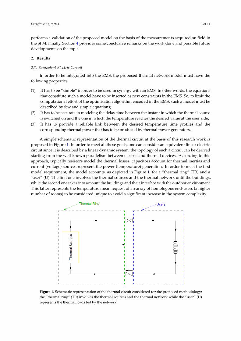
A simple schematic representation of the thermal circuit at the basis of this research work isproposed in Figure 1. In order to meet all these goals, one can consider an equivalent linear electriccircuit since it is described by a linear dynamic system; the topology of such a circuit can be derivedstarting from the well-known parallelism between electric and thermal devices. According to thisapproach, typically resistors model the thermal losses, capacitors account for thermal inertias andcurrent (voltage) sources represent the power (temperature) generation. In order to meet the firstmodel requirement, the model accounts, as depicted in Figure 1, for a “thermal ring” (TR) and a“user” (U). The first one involves the thermal sources and the thermal network until the buildings,while the second one takes into account the buildings and their interface with the outdoor environment.This latter represents the temperature mean request of an array of homologous end-users (a highernumber of rooms) to be considered unique to avoid a significant increase in the system complexity.

Energies 2016, 9, 914 3 of 15

the SPM. Finally, Section 4 provides some conclusive remarks on the work done and possible future developments on the topic.

2. Results

2.1. Equivalent Electric Circuit

In order to be integrated into the EMS, the proposed thermal network model must have the following properties:

(1) It has to be “simple” in order to be used in synergy with an EMS. In other words, the equations that constitute such a model have to be inserted as new constraints in the EMS. So, to limit the computational effort of the optimisation algorithm encoded in the EMS, such a model must be described by few and simple equations;

(2) It has to be accurate in modeling the delay time between the instant in which the thermal source is switched on and the one in which the temperature reaches the desired value at the user side;

(3) It has to provide a reliable link between the desired temperature time profiles and the corresponding thermal power that has to be produced by thermal power generators.

A simple schematic representation of the thermal circuit at the basis of this research work is proposed in Figure 1. In order to meet all these goals, one can consider an equivalent linear electric circuit since it is described by a linear dynamic system; the topology of such a circuit can be derived starting from the well-known parallelism between electric and thermal devices. According to this approach, typically resistors model the thermal losses, capacitors account for thermal inertias and current (voltage) sources represent the power (temperature) generation. In order to meet the first model requirement, the model accounts, as depicted in Figure 1, for a “thermal ring” (TR) and a “user” (U). The first one involves the thermal sources and the thermal network until the buildings, while the second one takes into account the buildings and their interface with the outdoor environment. This latter represents the temperature mean request of an array of homologous end-users (a higher number of rooms) to be considered unique to avoid a significant increase in the system complexity.

Figure 1. Schematic representation of the thermal circuit considered for the proposed methodology: the “thermal ring” (TR) involves the thermal sources and the thermal network while the “user” (U) represents the thermal loads fed by the network.

The choice of using an equivalent electric representation instead of a purely thermal one is driven by the fact that several EMS for microgrid applications are typically designed to manage the electric part of the grid. For this reason, if an electric equivalent of the system is provided, its

Figure 1. Schematic representation of the thermal circuit considered for the proposed methodology:the “thermal ring” (TR) involves the thermal sources and the thermal network while the “user” (U)represents the thermal loads fed by the network.

Energies 2016, 9, 914 4 of 14

The choice of using an equivalent electric representation instead of a purely thermal one is drivenby the fact that several EMS for microgrid applications are typically designed to manage the electricpart of the grid. For this reason, if an electric equivalent of the system is provided, its integration couldbe performed in a larger set of EMS tools and would also allow the management of thermal power tobe upgraded by retrofitting existing EMS structures.

The proposed equivalent circuit is depicted in Figure 2 and the circuital elements can be describedas follows:

• The current source I0 represents the thermal power generation;• The capacitance C0 accounts for the thermal inertia responsible for the time delay necessary to

obtain the desired temperature in the heat generator circuit;• The conductance G0 models the heat generator circuit losses;• The voltage source V0 models the fact that, without any thermal source, the heat generator

network temperature approaches the ground temperature;• The switch B1 models the possible disconnection between the generation and the load (encoded in

a Boolean variable S, true when B1 is open);• The diode D1 models the fact that the user cannot transfer heat to the water in the heat

generator circuit;• The conductance G11 accounts for the pipe thermal losses in the thermal circuits of the buildings;• The capacitance C1 accounts for the thermal inertia responsible for the time delay necessary to

obtain the desired temperature at the user side;• The conductance G1 represents the thermal losses, which depend on the user insulation;• The voltage V1 mimics the fact that, without any thermal source, the user temperature approaches

the outdoor ambient one.

In the proposed model, VC0 is the voltage between terminals A and B and represents the thermalring temperature, while VC1, which is the voltage between terminals A1 and B1, represents the usermean temperature.

Energies 2016, 9, 914 4 of 15

integration could be performed in a larger set of EMS tools and would also allow the management of thermal power to be upgraded by retrofitting existing EMS structures.

The proposed equivalent circuit is depicted in Figure 2 and the circuital elements can be described as follows:

• The current source I0 represents the thermal power generation; • The capacitance C0 accounts for the thermal inertia responsible for the time delay necessary to

obtain the desired temperature in the heat generator circuit; • The conductance G0 models the heat generator circuit losses; • The voltage source V0 models the fact that, without any thermal source, the heat generator

network temperature approaches the ground temperature; • The switch models the possible disconnection between the generation and the load (encoded

in a Boolean variable S, true when B1 is open); • The diode models the fact that the user cannot transfer heat to the water in the heat generator

circuit; • The conductance G11 accounts for the pipe thermal losses in the thermal circuits of the buildings; • The capacitance C1 accounts for the thermal inertia responsible for the time delay necessary to

obtain the desired temperature at the user side; • The conductance G1 represents the thermal losses, which depend on the user insulation; • The voltage V1 mimics the fact that, without any thermal source, the user temperature

approaches the outdoor ambient one.

In the proposed model, VC0 is the voltage between terminals A and B and represents the thermal ring temperature, while VC1, which is the voltage between terminals A1 and B1, represents the user mean temperature.

Figure 2. The proposed equivalent electrical circuit of the Smart Polygeneration Microgrid (SPM) thermal network (the green line denotes what has been labelled as TR and the blue one is the boundary of the user U).

Applying the Kirchoff’s laws to the circuit of Figure 2, one obtains the following set of two ordinary differential equations in the state variables VC0 and VC1:

( ) ( ) ( ) ( ) ( ) ( )0 0 11 11 110 1 0 1 0

0

0

0 0 0 0

1CC C B

dV t G G G GV t V t I t V t V tdt C C C C

GC

+= − + + + + (1)

( ) ( ) ( ) ( ) ( )1 11 1 11 110 1 1 1

1 1 1 1

1 CC C B

dV t G G G GV t V t V t G V tdt C C C C

+= − − + (2)

with initial conditions ( ) *0 0 0 C CV t V= and ( ) *

1 0 1C CV t V= at time t0. Here the voltage VB1 at the switch B1 is given by:

Figure 2. The proposed equivalent electrical circuit of the Smart Polygeneration Microgrid (SPM)thermal network (the green line denotes what has been labelled as TR and the blue one is the boundaryof the user U).

Applying the Kirchoff’s laws to the circuit of Figure 2, one obtains the following set of twoordinary differential equations in the state variables VC0 and VC1:

dVC0 (t)dt

= −G0 + G11

C0VC0 (t) +

G11

C0VC1 (t) +

1C0

I0 (t) +G11

C0VB1 (t) +

G0

C0V0 (t) (1)

Energies 2016, 9, 914 5 of 14

dVC1 (t)dt

=G11

C1VC0 (t)−

G1 + G11

C1VC1 (t)−

G11

C1VB1 (t) +

G1

C1V1 (t) (2)

with initial conditions VC0 (t0) = V∗C0 and VC1 (t0) = V∗C1 at time t0. Here the voltage VB1 at the switchB1 is given by:

VB1 (t) =

{VC0 (t)−VC1 (t) i f S (t) = true

0 i f S (t) = false(3)

The switch is therefore simulated using the Boolean variable S which is equal to one if the switchis open (e.g., during the night period when the TR is disconnected) and is equal to zero if the switchis closed. The numerical solution of (1), (2) allows finding out the time profile of both the TR and Utemperatures, given the thermal power generation (which meets the aforementioned requirements ofthe model).

2.2. Equivalent Electric Circuit Parameters Estimation

Once the topological layout of the network has been defined, it is necessary to define a procedureto evaluate the five parameters proposed by the model: three resistances and two capacitances.One possibility consists of considering the physical layout of the plant and proceeding with acharacterization of the elements that compose the system. Nevertheless, such a procedure iscomputationally complex and affected by uncertainties on the phenomena to be considered. Moreover,the model of the system varies in accordance to the specific thermal network, making difficult toobtain a general procedure to be extended for a generic microgrid asset. To overcome these problems,the methodology adopted in the present paper for parameters estimation relies on an optimizationprocedure that aims at minimizing the difference between the temperature time profile calculatedwith (1)–(3) and the measured one. Under this assumption, the only a priori hypothesis is the topologyof the circuit, which, by the way, can be judged in an ex-post evaluation comparing the calculated andthe measured outputs. The aim of the present section is to present the proposed optimization approach.

As measured temperatures and thermal powers are supposed to be known on a uniform samplingof the interval [t1, t2] according to a step ∆t and resulting in N = (t2 − t1) /∆t + 1 samples, the wholeproblem will be presented in a discrete form.

As far as the cost function is concerned, the χ2 function has been chosen, in order to have thepossibility of subjecting the obtained trends to a statistical evaluation (i.e., the so called chi-squaredtest [18] typically used to establish if a theoretical model is incompatible with a set of experimentalobservations). With specific reference to the available measurements, the cost function for the problemunder consideration can be written as:

χ2calc =

N

∑i=1

(VmeasC0 (ti)−VC0(ti))

2

σ2i,C0

+(Vmeas

C1 (ti)−VC1(ti))2

σ2i,C1

(4)

being σi,C0 and σi,C1 the standard deviation of the measured temperature of the thermal ring VmeasC0

and of the user VmeasC1 , respectively.

The constraints of the problem are the discretized versions of (1) and (2), i.e.,

VC0(ti+1)∆t = VC0 (ti)

(1

∆t −G0+G11

C0

)VC0 (ti) +

G11C0

VC1 (ti) +1

C0I0 (ti) +

G11C0

VB1 (ti) +G0C0

V0 (ti) (5)

andVC1 (ti+1)

∆t=

G11

C1VC0 (ti) +

(1

∆t− G1 + G11

C1

)VC1 (ti)−

G11

C1VB1 (ti) +

G1

C1V1 (ti) (6)

The five unknown parameters must belong to reasonable ranges that can be estimated withphysical considerations (e.g., the initial estimation of capacitance C0 can be obtained by the waterspecific heat multiplied by the overall water mass flowing in the thermal ring).

Energies 2016, 9, 914 6 of 14

Moreover, the defined optimization procedure does not require the parameters to be time invariant.As a matter of fact, it seems to be reasonable that they may vary with time in accordance with thespecific usage conditions of the rooms (e.g., the number of occupants in a room or the people flowingfrom one place to another have an impact on the efficiency and inertia of the system). This suggests thepossibility of dividing the optimization horizon into time slots, according to the habits of the districtfed by the considered thermal network.

Once the optimization problem has been set up, it is necessary to define an algorithm to identifythe optimal solution (parameters) to fit the measured data with the proposed model. This is not an easytask, as the cost function (4) that has to be minimized is not a polynomial (the two capacitances appearat the denominator after having inserted (5) and (6) into (4)). To address this problem, a stochasticoptimization algorithm has to be preferred in order to avoid possible local minima: the Ant ColonyOptimization algorithm (ACO) [19] encodes this characteristic in its nature. In the ACO algorithm,two degrees of freedom are left to the users in order to increase the velocity of convergence and/oremphasize its accuracy. However, to reduce the effect of an inappropriate choice, a different version ofthe ACO algorithm has here been adopted: the Multivariate Ant Colony Algorithm for ContinuousOptimization (MACACO) [20]. MACACO is an extension of ACO based on a covariance matrixinstead of a simple variance vector (adopted in ACO).

The updating step for each ant is made such that the new distribution of the solutions points at thepromising region is supposedly indicated by the candidate solutions at the previous iteration. This goalcan be achieved recalculating this matrix using just 70% of the best solutions found at the presentiteration (the 70% value is defined on empirical basis). By doing that, the obtained distribution will goon until the covariance tends to almost zero and is going to be centered at the best optima found.

2.3. Equivalent Electric Circuit Parameters Estimation

The typical thermal network characterization inserted in a microgrid EMS consists of providingthe optimization procedure with a constraint stating that the overall thermal power generation must beat least equal to the thermal request (expressed in terms of thermal power) over the optimization timehorizon. Unfortunately, this implies to know in advance the time profile of the thermal power request,which is typically predicted by means of the persistency method [21]. This produces a significantamount of uncertainty affecting the overall EMS result.

One of the most interesting applications of the proposed model, for a cogenerative microgrid,is the possibility of integration into an EMS in order to make it able to process the request in termsof temperature profile, which seems much easier to forecast. It is intuitive that for a given loadtemperature profile, the optimal solution from an economic point of view is given by achieving theminimum amount of primary energy (current in the equivalent modeling) able to guarantee that theroom temperature is equal or greater than the desired one.

Recalling the meaning of the electric-thermal equivalency of circuital quantities, it is possible toexpress the cost function in terms of the I0 current. In other words, the optimal solution corresponds tothe values of I0(t) that minimize the overall thermal energy in a finite time horizon Nt, i.e.,

minNt

∑i=1

I0 (ti)∆t (7)

constrained by (5) and (6) and such that:

VC1(ti) ≥ VdesC1 (ti) ∀i = 1, . . . , Nt (8)

VdesC1 (ti) being the desired value of the load temperature at time ti.

Energies 2016, 9, 914 7 of 14

3. Discussion

3.1. Model Validation in the SPM

This section reports the results obtained by applying the proposed model to the Savona CampusSPM. A complete description of the SPM has been provided in [7,22], but, from a pure thermal point ofview, it is worth recalling the SPM’s main features:

• two Combined Heat and Power Gas Turbines (CHP-GT) Capstone C65 model, able to generate65 kW (electric power) and 112 kW (thermal power);

• one CHP-GT Capstone C30 able to generate 30 kW (electric power) and 55 kW (thermal power);• two gas boilers characterized by a rated thermal power of 500 kW per boiler.

Figure 3 sketches the SPM map, where a green line groups the TR (composed by the networkconnections, in red, and the thermal sources, in orange) and the set of blue lines denotes the U(the different buildings). The thermal network is fed by the three cogeneration gas turbines and twogas boilers. The pipes are installed underground and are properly insulated in order to minimizeheat losses; the pipe diameters are in the range between DN80 and DN125. Figure 3 does not showthe pipes that distribute heat inside each building, where hot water is moved by on/off centrifugalpumps and heat is transferred to the indoor air by means of radiators or fan coils. During winterdays, the Campus thermal load can be up to 900 kW of peak request and the thermal energy yearlyconsumption is about 1300 MWh.

Energies 2016, 9, 914 7 of 15

• two Combined Heat and Power Gas Turbines (CHP-GT) Capstone C65 model, able to generate 65 kW (electric power) and 112 kW (thermal power);

• one CHP-GT Capstone C30 able to generate 30 kW (electric power) and 55 kW (thermal power); • two gas boilers characterized by a rated thermal power of 500 kW per boiler.

Figure 3 sketches the SPM map, where a green line groups the TR (composed by the network connections, in red, and the thermal sources, in orange) and the set of blue lines denotes the U (the different buildings). The thermal network is fed by the three cogeneration gas turbines and two gas boilers. The pipes are installed underground and are properly insulated in order to minimize heat losses; the pipe diameters are in the range between DN80 and DN125. Figure 3 does not show the pipes that distribute heat inside each building, where hot water is moved by on/off centrifugal pumps and heat is transferred to the indoor air by means of radiators or fan coils. During winter days, the Campus thermal load can be up to 900 kW of peak request and the thermal energy yearly consumption is about 1300 MWh.

The heating network is monitored in real time by the SPM control room by means of on-field sensors that allow the following variables to be measured: the water mass flow rate, the supply and return lines temperatures, the thermal power output of each gas turbine and boiler and the outdoor temperature. At present, the buildings (U) are not equipped with any sensor measuring the indoor conditions as well as the water temperature and flow rate, so that it is possible to evaluate only the overall thermal load of the Campus but not the single building ones. In the future, each building will be equipped with sensors in order to develop more accurate analyses and to highlight criticalities of the thermal network. However, the rooms’ temperatures have been recorded in the data collection period by means of portable indoor temperature monitoring systems (Elitech RC-4 Mini Temperature Data Logger by Jiangsu Jingchuang Electronics Co. Ltd., Xuzhou, China, 2015 [23]).

Figure 3. The SPM layout with the highlight of the “thermal ring” (the union of the thermal sources and the thermal network) and the “user” (the set of buildings involved).

As mentioned, in order to attain the goals of the work here presented, a proper set of experimental data had to be collected, on the base of which identifying the model parameters and performing the consistency estimation.

Furthermore, as specified before, the representation of the thermal network has been based on the introduction of an “equivalent” unique end-user U, despite of the large number of actual physical loads. As a consequence, the proper choice of the rooms in which to carry on the temperature measurements had to be identified. In our case, the logic was that of performing the temperature survey within rooms that, even if included in buildings with non-perfectly superimposable thermal

Figure 3. The SPM layout with the highlight of the “thermal ring” (the union of the thermal sourcesand the thermal network) and the “user” (the set of buildings involved).

The heating network is monitored in real time by the SPM control room by means of on-fieldsensors that allow the following variables to be measured: the water mass flow rate, the supply andreturn lines temperatures, the thermal power output of each gas turbine and boiler and the outdoortemperature. At present, the buildings (U) are not equipped with any sensor measuring the indoorconditions as well as the water temperature and flow rate, so that it is possible to evaluate only theoverall thermal load of the Campus but not the single building ones. In the future, each building willbe equipped with sensors in order to develop more accurate analyses and to highlight criticalities ofthe thermal network. However, the rooms’ temperatures have been recorded in the data collectionperiod by means of portable indoor temperature monitoring systems (Elitech RC-4 Mini TemperatureData Logger by Jiangsu Jingchuang Electronics Co. Ltd., Xuzhou, China, 2015 [23]).

Energies 2016, 9, 914 8 of 14

As mentioned, in order to attain the goals of the work here presented, a proper set of experimentaldata had to be collected, on the base of which identifying the model parameters and performing theconsistency estimation.

Furthermore, as specified before, the representation of the thermal network has been based on theintroduction of an “equivalent” unique end-user U, despite of the large number of actual physical loads.As a consequence, the proper choice of the rooms in which to carry on the temperature measurementshad to be identified. In our case, the logic was that of performing the temperature survey within roomsthat, even if included in buildings with non-perfectly superimposable thermal characteristics, could beconsidered as homologous under the temperature requirements of the occupants (offices, apartments,classrooms). In the choice of the rooms to be monitored, particular attention has been devoted inevaluating how the human behaviors (windows opening, room thermostat adjustments, etc.) couldaffect the thermal profiles within the rooms, trying to minimize these uncontrollable variables.

Operatively, along the survey period the indoor temperature, within the selected rooms, has beenacquired continuously and the obtained trends have been recorded weekly. By averaging the datacollected in the selected users, a set of day-by-day temperature trends (and the related standarddeviations), each of which assumed as representative of the typical user (i.e., room) served by thethermal network, has been obtained.

3.2. Parameter Characterization

The parameters characterization was conducted during the winter season in the period betweenJanuary 2016 and March 2016. Measurement campaigns were carried out three days per week(Monday and Friday have been avoided because the thermal behavior of the system is influenced inthose days by the fact that during weekend the heating system of the whole campus is switched off).The SPM thermal behavior was divided into three different time frames (each one object of parameteridentification):

(a) Time Frame 1: from 10 p.m. to 6 a.m. when the thermal ring stops working and people’s presenceinside the buildings is extremely reduced;

(b) Time Frame 2: from 6 a.m. to 5 p.m. when the building pumping system works and a significantnumber of people are present inside the buildings;

(c) Time Frame 3: from 5 p.m. to 10 p.m. when some loads are disconnected from the thermalnetwork and gradually fewer people are present.

As explained before, this suggests considering the circuit parameters as piecewise constantfunctions throughout the day, i.e.,

Gi (t) =

Gi,1 if 6 a.m. ≤ t < 5 p.m.

Gi,2 if 5 p.m. ≤ t < 10 p.m.

Gi,3 if 10 p.m. ≤ t ≤ 5 a.m.

i ∈ {0, 1, 2} (9)

Ci (t) =

Ci,1 if 6 a.m. ≤ t < 5 p.m.

Ci,2 if 5 p.m. ≤ t < 10 p.m.

Ci,3 if 10 p.m. ≤ t ≤ 5 a.m.

i ∈ {0, 1} (10)

Moreover, condition S(t) becomes true if:

• 0 a.m. ≤ t ≤ 6 a.m. or 10 p.m. ≤ t ≤ 12 p.m., in order to encode condition (a);• VC0(t) < VC1(t), in order to encode the presence of the diode D1;• VC1(t) > VC1,max(t), where VC1,max(t) is the user maximum temperature allowed at the instant t.

Once all the measurements were acquired, two thirds of the measurement data were used to trainthe model (identifying the parameters) while the other third has been used to test the performances

Energies 2016, 9, 914 9 of 14

of the parameters found. In more detail, data acquired on Tuesday and Thursday of each week wereused to choose the optimal values of the parameters, while Wednesday’s data were used for theverification. This choice was made in order to have uniformity in both the identification and validationon the results. The tests have been performed taking the input measurements (ground temperature,environmental temperature and thermal power from the heating ring), calculating the U temperatureusing the model and then comparing the calculated results with the measured ones.

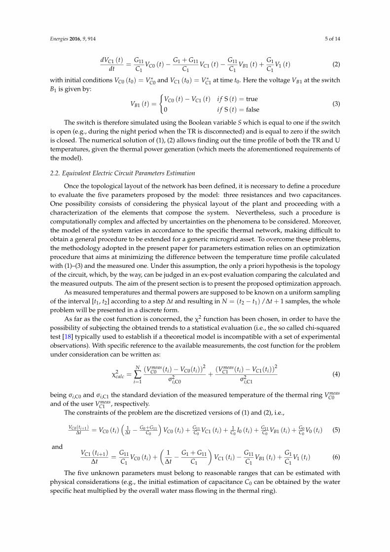
The optimal values of the circuit parameter (which minimize the cost function) are reported inTable 1 (all the data used to find the parameter reported in Table 1 are available at Savona Campus andcan be provided at request).

Table 1. Optimal Parameters Values.

Parameter 6 a.m.–5 p.m. 5 p.m.–10 p.m. 10 p.m.–6 a.m.

G0 (kW/K) 2.58 3.72 0.40C0 (kJ/K) 0.93 × 105 2.26 × 105 1.73 × 105

G1 (kW/K) 28.76 24.03 50.01C1 (kJ/K) 3.91 × 106 3.17 × 106 3.11 × 106

G11 (kW/K) 3.62 20.00 4.01

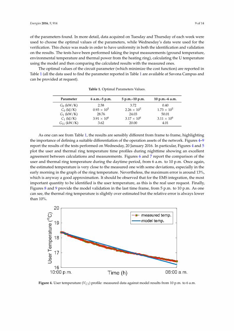
As one can see from Table 1, the results are sensibly different from frame to frame, highlightingthe importance of defining a suitable differentiation of the operation assets of the network. Figures 4–9report the results of the tests performed on Wednesday, 20 January 2016. In particular, Figures 4 and 5plot the user and thermal ring temperature time profiles during nighttime showing an excellentagreement between calculations and measurements. Figures 6 and 7 report the comparison of theuser and thermal ring temperature during the daytime period, from 6 a.m. to 10 p.m. Once again,the estimated temperature is very close to the measured one with some deviations, especially in theearly morning in the graph of the ring temperature. Nevertheless, the maximum error is around 13%,which is anyway a good approximation. It should be observed that for the EMS integration, the mostimportant quantity to be identified is the user temperature, as this is the real user request. Finally,Figures 8 and 9 provide the model validation in the last time frame, from 5 p.m. to 10 p.m. As onecan see, the thermal ring temperature is slightly over estimated but the relative error is always lowerthan 10%.

Energies 2016, 9, 914 9 of 15

Table 1. Optimal Parameters Values.

Parameter 6 a.m.–5 p.m. 5 p.m.–10 p.m. 10 p.m.–6 a.m. G0 (kW/K) 2.58 3.72 0.40 C0 (kJ/K) 0.93 × 105 2.26 × 105 1.73 × 105

G1 (kW/K) 28.76 24.03 50.01 C1 (kJ/K) 3.91 × 106 3.17 × 106 3.11 × 106

G11 (kW/K) 3.62 20.00 4.01

As one can see from Table 1, the results are sensibly different from frame to frame, highlighting the importance of defining a suitable differentiation of the operation assets of the network. Figures 4–9 report the results of the tests performed on Wednesday, 20 January 2016. In particular, Figures 4 and 5 plot the user and thermal ring temperature time profiles during nighttime showing an excellent agreement between calculations and measurements. Figures 6 and 7 report the comparison of the user and thermal ring temperature during the daytime period, from 6 a.m. to 10 p.m. Once again, the estimated temperature is very close to the measured one with some deviations, especially in the early morning in the graph of the ring temperature. Nevertheless, the maximum error is around 13%, which is anyway a good approximation. It should be observed that for the EMS integration, the most important quantity to be identified is the user temperature, as this is the real user request. Finally, Figures 8 and 9 provide the model validation in the last time frame, from 5 p.m. to 10 p.m. As one can see, the thermal ring temperature is slightly over estimated but the relative error is always lower than 10%.

Figure 4. User temperature (VC1) profile: measured data against model results from 10 p.m. to 6 a.m.

Use

r T

empe

ratu

re (

oC

)

Figure 4. User temperature (VC1) profile: measured data against model results from 10 p.m. to 6 a.m.

Energies 2016, 9, 914 10 of 14Energies 2016, 9, 914 10 of 15

Figure 5. Ring temperature (VC0) profile: measured data against model results from 10 p.m. to 6 a.m.

Figure 6. User temperature (VC1) profile: measured data against model results from 6 a.m. to 5 p.m.

Figure 7. Ring temperature (VC0) profile: measured data against model results from 6 a.m. to 5 p.m.

Rin

g T

empe

ratu

re (

oC

)U

ser

Tem

pera

ture

(oC

)R

ing

Tem

pera

ture

(oC

)

Figure 5. Ring temperature (VC0) profile: measured data against model results from 10 p.m. to 6 a.m.

Energies 2016, 9, 914 10 of 15

Figure 5. Ring temperature (VC0) profile: measured data against model results from 10 p.m. to 6 a.m.

Figure 6. User temperature (VC1) profile: measured data against model results from 6 a.m. to 5 p.m.

Figure 7. Ring temperature (VC0) profile: measured data against model results from 6 a.m. to 5 p.m.

Rin

g T

empe

ratu

re (

oC

)U

ser

Tem

pera

ture

(oC

)R

ing

Tem

pera

ture

(oC

)

Figure 6. User temperature (VC1) profile: measured data against model results from 6 a.m. to 5 p.m.

Energies 2016, 9, 914 10 of 15

Figure 5. Ring temperature (VC0) profile: measured data against model results from 10 p.m. to 6 a.m.

Figure 6. User temperature (VC1) profile: measured data against model results from 6 a.m. to 5 p.m.

Figure 7. Ring temperature (VC0) profile: measured data against model results from 6 a.m. to 5 p.m.

Rin

g T

empe

ratu

re (

oC

)U

ser

Tem

pera

ture

(oC

)R

ing

Tem

pera

ture

(oC

)

Figure 7. Ring temperature (VC0) profile: measured data against model results from 6 a.m. to 5 p.m.

Energies 2016, 9, 914 11 of 14Energies 2016, 9, 914 11 of 15

Figure 8. User temperature (VC1) profile: measured data against model results from 5 p.m. to 10 p.m.

Figure 9. Ring temperature (VC0) profile: measured data against model results from 5 p.m. to 10 p.m.

In order to have an overall evaluation of the accuracy of the proposed model, the value of the chi-squared function has been calculated for the shown testing period and compared to the chi-squared distribution at level α for determining the goodness of fit [15]. To determine the degrees of freedom (d.o.f.) of the chi-squared distribution, it is necessary to consider the total number of acquired measurements (n) and subtracts the number of estimated parameters (in our case 5). The test statistic follows, approximately, a chi-square distribution with (n − 5) degrees of freedom. The more the chi-squared calculated is lower than the chi-squared distribution at level α = 0.95, the more accurate is the result. Moreover, deciding whether a model is in accordance with the data is often summarized by the p-value. According to [24], the more the p-value is close to 1 the more the model is accurate. In Table 2 the numerical values of all the introduced indicators are reported: the fact that the reference chi-square value is always greater than the calculated one and, in particular, that the p-value extremely close to 1 indicates the high accuracy of the model in describing the thermal phenomena.

Use

r T

empe

ratu

re (

oC

)

05:00 p.m. 10:00 p.m.Time (h)45

50

55

60

65

70

Rin

g T

empe

ratu

re (

oC

)

Measured temp.Model temp.

Figure 8. User temperature (VC1) profile: measured data against model results from 5 p.m. to 10 p.m.

Energies 2016, 9, 914 11 of 15

Figure 8. User temperature (VC1) profile: measured data against model results from 5 p.m. to 10 p.m.

Figure 9. Ring temperature (VC0) profile: measured data against model results from 5 p.m. to 10 p.m.

In order to have an overall evaluation of the accuracy of the proposed model, the value of the chi-squared function has been calculated for the shown testing period and compared to the chi-squared distribution at level α for determining the goodness of fit [15]. To determine the degrees of freedom (d.o.f.) of the chi-squared distribution, it is necessary to consider the total number of acquired measurements (n) and subtracts the number of estimated parameters (in our case 5). The test statistic follows, approximately, a chi-square distribution with (n − 5) degrees of freedom. The more the chi-squared calculated is lower than the chi-squared distribution at level α = 0.95, the more accurate is the result. Moreover, deciding whether a model is in accordance with the data is often summarized by the p-value. According to [24], the more the p-value is close to 1 the more the model is accurate. In Table 2 the numerical values of all the introduced indicators are reported: the fact that the reference chi-square value is always greater than the calculated one and, in particular, that the p-value extremely close to 1 indicates the high accuracy of the model in describing the thermal phenomena.

Use

r T

empe

ratu

re (

oC

)

05:00 p.m. 10:00 p.m.Time (h)45

50

55

60

65

70

Rin

g T

empe

ratu

re (

oC

)

Measured temp.Model temp.

Figure 9. Ring temperature (VC0) profile: measured data against model results from 5 p.m. to 10 p.m.

In order to have an overall evaluation of the accuracy of the proposed model, the value ofthe chi-squared function has been calculated for the shown testing period and compared to thechi-squared distribution at level α for determining the goodness of fit [15]. To determine the degrees offreedom (d.o.f.) of the chi-squared distribution, it is necessary to consider the total number of acquiredmeasurements (n) and subtracts the number of estimated parameters (in our case 5). The test statisticfollows, approximately, a chi-square distribution with (n − 5) degrees of freedom. The more thechi-squared calculated is lower than the chi-squared distribution at level α = 0.95, the more accurate isthe result. Moreover, deciding whether a model is in accordance with the data is often summarizedby the p-value. According to [24], the more the p-value is close to 1 the more the model is accurate.In Table 2 the numerical values of all the introduced indicators are reported: the fact that the referencechi-square value is always greater than the calculated one and, in particular, that the p-value extremelyclose to 1 indicates the high accuracy of the model in describing the thermal phenomena.

Table 2. Statistics on the testing period.

Timeslot χ2calc p-Value χ2 (95%) dof

6 a.m.–5 p.m. 14.8 ~1 39.8 565 p.m.–10 p.m. 7.42 ~1 92.1 11610 p.m.–6 a.m. 9.00 ~1 68.3 89

Energies 2016, 9, 914 12 of 14

3.3. Validation of the EMS Integration

Finally, the proposed model has been implemented in the SPM control system in order to integrateit into the microgrid EMS. The experiment has been performed providing the EMS with the measuredtemperature and assuming it as the desired temperature; the EMS produced, as output, the thermalpower to be provided by the heating units in order to meet the temperature request and minimizingthe overall energy over the time horizon. The power request profile is then compared to the realpower generation recorded by the SPM Supervisory Control And Data Acquisition (SCADA) system,managed in accordance to the following rules based on the ring temperature T:

• if T < 49 ◦C, then both boilers switch on• if 49 ◦C < T < 53 ◦C, then only one boiler switches on• if T > 53 ◦C, then both boilers switch off

Figure 10 provides the comparison of the thermal power obtained by the EMS (black one) and theactual thermal power profile (red dashed line). As can be noted, the optimal power profile is smotherand more constant, providing a saving equal to 1400 kWh along the analyzed 24 h, corresponding tothe 12.7% of the total thermal energy requested in the whole day (integrating the thermal power redcurve of Figure 10 one obtains 11,050 kWh). From an economical point of view, considering a mean costof the thermal energy of 0.096 €/kWh (which is the case of the SPM), it is possible to calculate the dailysavings as €134 against a total € cost of the non-optimized scenario of €1061. Finally, Figure 11 shows:

i. the measured temperature (red dotted line);ii. the temperature calculated feeding the model (1)–(3) with the optimal thermal power profile

(black solid line);iii. the temperature calculated feeding the model (1)–(3) with the measured thermal power profile

(blue dash-dotted line).

Energies 2016, 9, 914 12 of 15

Table 2. Statistics on the testing period.

Timeslot p-Value (95%) dof 6 a.m.–5 p.m. 14.8 ~1 39.8 56

5 p.m.–10 p.m. 7.42 ~1 92.1 116 10 p.m.–6 a.m. 9.00 ~1 68.3 89

3.3. Validation of the EMS Integration

Finally, the proposed model has been implemented in the SPM control system in order to integrate it into the microgrid EMS. The experiment has been performed providing the EMS with the measured temperature and assuming it as the desired temperature; the EMS produced, as output, the thermal power to be provided by the heating units in order to meet the temperature request and minimizing the overall energy over the time horizon. The power request profile is then compared to the real power generation recorded by the SPM Supervisory Control And Data Acquisition (SCADA) system, managed in accordance to the following rules based on the ring temperature T:

• if T < 49 °C, then both boilers switch on • if 49 °C < T < 53 °C, then only one boiler switches on • if T > 53 °C, then both boilers switch off

Figure 10 provides the comparison of the thermal power obtained by the EMS (black one) and the actual thermal power profile (red dashed line). As can be noted, the optimal power profile is smother and more constant, providing a saving equal to 1400 kWh along the analyzed 24 h, corresponding to the 12.7% of the total thermal energy requested in the whole day (integrating the thermal power red curve of Figure 10 one obtains 11,050 kWh). From an economical point of view, considering a mean cost of the thermal energy of 0.096 €/kWh (which is the case of the SPM), it is possible to calculate the daily savings as €134 against a total € cost of the non-optimized scenario of €1061. Finally, Figure 11 shows:

i. the measured temperature (red dotted line); ii. the temperature calculated feeding the model (1)–(3) with the optimal thermal power profile

(black solid line); iii. the temperature calculated feeding the model (1)–(3) with the measured thermal power profile

(blue dash-dotted line).

Figure 10. Power daily profile: optimal profile versus real profile.

The

rmal

Pow

er (

kW)

Figure 10. Power daily profile: optimal profile versus real profile.

This allows us to draw the following conclusions: (a) the comparison between (i) and (ii) showsthat the optimal solution is able to reproduce the desired temperature; (b) the good superpositionbetween (i) and (iii) validates once again the effectiveness of the equivalent circuit, as, when fed by thereal power, it is able to predict the correct time profile of the temperature; finally, (c) the comparativeanalysis of (ii) and (iii) states that there can be many different power injections that produce verysimilar temperature profiles, thus supporting the need to determine the most convenient one.

Energies 2016, 9, 914 13 of 14Energies 2016, 9, 914 13 of 15

Figure 11. Room temperature comparison (measured against calculated applying the model fed with the optimal and the measured power profile).

This allows us to draw the following conclusions: (a) the comparison between (i) and (ii) shows that the optimal solution is able to reproduce the desired temperature; (b) the good superposition between (i) and (iii) validates once again the effectiveness of the equivalent circuit, as, when fed by the real power, it is able to predict the correct time profile of the temperature; finally, (c) the comparative analysis of (ii) and (iii) states that there can be many different power injections that produce very similar temperature profiles, thus supporting the need to determine the most convenient one.

4. Conclusions

The aim of this contribution has been to propose a simple but general model of a thermal network by means of an equivalent electric circuit. The aim of the present model is to be sufficiently accurate but also simple in order to be integrated into cogenerative microgrid EMSs. The main task of this model is that of linking the thermal power request of the load (usually provided as an input the EMS) to the user temperature (a more meaningful desired parameter for the user). The model proposed is based on a linear equivalent electric circuit whose main parameters can be determined through a measurement campaign applying a parameter identification optimal procedure. The proposed model has been tested in the Savona Campus Smart Polygeneration Microgrid thermal network, in order to show the actual applicability and robustness of the procedure. The values of the parameters involved have been computed by means of an optimization procedure that, in practice, minimizes the difference between the temperature profiles of the thermal circuit and of the user as calculated with the proposed model and the measured ones. The obtained numerical results show that the model describes in a very accurate way the set of measured temperatures and, at the same time, can be easily used as a procedure to optimally schedule the thermal power production leading, to significant thermal energy savings.

Author Contributions: Renato Procopio, Federico Delfino and Alessandro Nilberto developed the equivalent electric modeling of the thermal network; Andrea Bonfiglio and Massimo Brignone performed the experimental validation and the EMS integration; Andrea Bonfiglio wrote the paper.

Conflicts of Interest: The authors declare no conflict of interest.

References

Use

r T

empe

ratu

re (

oC

)

Figure 11. Room temperature comparison (measured against calculated applying the model fed withthe optimal and the measured power profile).

4. Conclusions

The aim of this contribution has been to propose a simple but general model of a thermal networkby means of an equivalent electric circuit. The aim of the present model is to be sufficiently accuratebut also simple in order to be integrated into cogenerative microgrid EMSs. The main task of thismodel is that of linking the thermal power request of the load (usually provided as an input the EMS)to the user temperature (a more meaningful desired parameter for the user). The model proposedis based on a linear equivalent electric circuit whose main parameters can be determined through ameasurement campaign applying a parameter identification optimal procedure. The proposed modelhas been tested in the Savona Campus Smart Polygeneration Microgrid thermal network, in order toshow the actual applicability and robustness of the procedure. The values of the parameters involvedhave been computed by means of an optimization procedure that, in practice, minimizes the differencebetween the temperature profiles of the thermal circuit and of the user as calculated with the proposedmodel and the measured ones. The obtained numerical results show that the model describes in a veryaccurate way the set of measured temperatures and, at the same time, can be easily used as a procedureto optimally schedule the thermal power production leading, to significant thermal energy savings.

Author Contributions: Renato Procopio, Federico Delfino and Alessandro Nilberto developed the equivalentelectric modeling of the thermal network; Andrea Bonfiglio and Massimo Brignone performed the experimentalvalidation and the EMS integration; Andrea Bonfiglio wrote the paper.

Conflicts of Interest: The authors declare no conflict of interest.

References

1. Palma-Behnke, R.; Benavides, C.; Lanas, F.; Severino, B.; Reyes, L.; Llanos, J.; Sáez, D. A microgrid energymanagement system based on the rolling horizon strategy. IEEE Trans. Smart Grids 2013, 4, 996–1006.[CrossRef]

2. Hatziargyriou, N. Microgrids—Large Scale Integration of Micro-Generation to Low Voltage Grids; Paper C6-309 inCigrè Biennial Section; Cigré: Paris, France, 2006.

3. Vasquez, J.C.; Guerrero, J.M.; Miret, J.; Castilla, M.; de Vicuña, L.G. Hierarchical control of intelligentmicrogrids. IEEE Ind. Electron. Mag. 2010, 4, 23–29. [CrossRef]

4. Bonfiglio, A.; Brignone, M.; Delfino, F.; Invernizzi, M.; Pampararo, F.; Procopio, R. A technique for theoptimal control and operation of grid-connected photovoltaic production units. In Proceedings of the 201247th International Universities Power Engineering Conference (UPEC), London, UK, 4–7 September 2012;pp. 1–6.

Energies 2016, 9, 914 14 of 14

5. Nikkhajoei, H.; Iravani, R. Steady-state model and power flow analysis of electronically-coupled distributedresource units. IEEE Trans. Power Deliv. 2007, 22, 721–728. [CrossRef]

6. Palensky, P.; Dietrich, D. Demand side management: Demand response, intelligent energy systems andsmart loads. IEEE Trans. Ind. Inf. 2011, 7, 381–388. [CrossRef]

7. Bonfiglio, A.; Barillari, L.; Bracco, S.; Brignone, M.; Delfino, F.; Pampararo, F.; Procopio, R.; Robba, M.;Rossi, M. An Optimization Algorithm for the Operation Planning of the University of Genoa SmartPolygeneration Microgrid. In Proceedings of the IREP 2013 Symposium-Bulk Power System Dynamics andControl—IX, Rethymnon, Greece, 25–30 August 2013.

8. Chen, Q.; Fu, R.; Xu, Y. Electrical circuit analogy for heat transfer analysis and optimization in heat exchangernetworks. Appl. Energy 2015, 139, 81–92. [CrossRef]

9. Kämpf, J.H.; Robinson, D. A simplified thermal model to support analysis of urban resources flows.Energy Build. 2007, 39, 445–453. [CrossRef]

10. Fraisse, G.; Viardot, C.; Lafabrie, O.; Achard, G. Development of a simplified and accurate building modelbased on electrical analogy. Energy Build. 2002, 34, 1017–1031. [CrossRef]

11. Aringhieri, R.; Malucelli, F. Optimal operations management and network planning of a district heatingsystem with a combined heat and power plant. Ann. Oper. Res. 2003, 120, 173–199. [CrossRef]

12. Rezaie, B.; Rosen, M.A. District heating and cooling: Review of technology and potential enhancements.Appl. Energy 2012, 93, 2–10. [CrossRef]

13. Larsen, H.V.; Palsson, H.; Bohn, B.; Ravn, H.F. Aggregated dynamic simulation model of district heatingnetworks. Energy Convers. Manag. 2002, 43, 995–1019. [CrossRef]

14. Kuosa, M.; Kontu, K.; Makila, T.; Lampinen, M.; Lahdelma, R. Static study of traditional and ring networksand the use of mass flow control in district heating applications. Appl. Ther. Eng. 2013, 54, 450–459.[CrossRef]

15. Haikarainen, C.; Pettersson, F.; Saxen, H. An MILP model for distributed energy system optimization.Chem. Eng. Trans. 2013, 35, 295–300.

16. Bracco, S.; Dentici, G.; Siri, S. Economic and environmental optimization model for the design and theoperation of a combined heat and power distributed generation system in an urban area. Energy 2013, 55,1014–1024. [CrossRef]

17. Wakui, T.; Kinoshita, T.; Yokoyama, R. A mixed-integer linear programming approach for cogeneration-basedresidential energy supply networks with power and heat interchanges. Energy 2014, 68, 29–46. [CrossRef]

18. Banks, J.; Carson, J.S.; Nelson, B.L.; Nicol, D.M. Discrete-Event System Simulation, 5th ed.; Pearson:Upper Saddle River, NJ, USA, 2010.

19. Dorigo, M.; Gambardella, L.M. Ant colony system: A cooperative learning approach to the travellingsalesman problem. IEEE Trans. Evol. Comput. 1997, 1, 53–66. [CrossRef]

20. De Franca, F.O.; Coelho, G.P.; Von Zuben, F.J.; Attux, R.R. Multivariate Ant Colony Optimization inContinuous Search Spaces. In Proceedings of the 10th Annual Conference on Genetic and EvolutionaryComputation, Atlanta, GA, USA, 12–16 July 2008; ACM: New York, NY, USA, 2008; pp. 9–16.

21. Beyer, H.; Martínez, J.; Suri, M.; Torres, J.; Lorenz, E.; Müller, S.; Hoyer-Klick, C.; Ineichen, P. Report onBenchmarking of Radiation Products. Sixth Framework Programme MESOR, Management and Exploitationof Solar Resource Knowledge. 2009. Available online: http://www.mesor.org/docs/MESoR_Benchmarking_of_radiation_products.pdf (accessed on 3 October 2016).

22. Barillari, L.; Bonfiglio, A.; Delfino, F.; Pampararo, F.; Procopio, R.; Rossi, M. The Smart PolygenerationMicrogrid Test-Bed Facility of Genoa University. In Proceedings of the 2012 47th International UniversitiesPower Engineering Conference (UPEC), London, UK, 4–7 September 2012; pp. 1–6.

23. Temperature Data Logger Feature. Available online: http://www.elitech.uk.com/news/Elitech_RC_4_temperature_data_logger_usb_data_logger_67.html. (accessed on 3 October 2016).

24. Beaujean, F.; Caldwell, A.; Kollár, D.; Kröninger, K. P-values for model evaluation. Phys. Rev. D 2011,83, 012004. [CrossRef]

© 2016 by the authors; licensee MDPI, Basel, Switzerland. This article is an open accessarticle distributed under the terms and conditions of the Creative Commons Attribution(CC-BY) license (http://creativecommons.org/licenses/by/4.0/).