i EXPERIMENTAL VALIDATION OF TURBOMACHINERY BLADE ...
264
i EXPERIMENTAL VALIDATION OF TURBOMACHINERY BLADE VIBRATION PREDICTIONS A thesis submitted to the University of London for the degree of Doctor of Philosophy By brahim Ata SEVER Department of Mechanical Engineering Imperial College London March, 2004
-
Upload
nguyenkhanh -
Category
Documents
-
view
233 -
download
5
Transcript of i EXPERIMENTAL VALIDATION OF TURBOMACHINERY BLADE ...

i
EXPERIMENTAL VALIDATION OF TURBOMACHINERY BLADE
VIBRATION PREDICTIONS
A thesis submitted to the University of London for the degree of Doctor of Philosophy
By brahim Ata SEVER
Department of Mechanical Engineering Imperial College London
March, 2004

ii
To my dear mother
erife SEVER
iii
Abstract
Bladed disk vibration amplitudes are known to be seriously amplified and varied from blade to blade due to the scatter in the blade geometry or due to variations in material properties. The phenomenon of having non-identical blades due to these variations is called mistuning. Since mistuning can lead to forced response amplitudes which are much larger than those predicted for a tuned assembly, additional dissipation elements (e.g., friction dampers) are sometimes integrated into the bladed disk assembly. The problem of controlling and predicting the vibration amplitudes of bladed disks has been a primary concern of many research studies. As a result several numerical models have been developed to represent the bladed disk assemblies to facilitate prediction of the relevant behaviour. Since so much depends on the reliability of these components, however, manufacturers are disinclined to use these models, however complicated, in their designs unless or until they are proved to be accurate representations of the real behaviour. In other words, the model proposed must demonstrably be capable of predicting the response of the real bladed disk within the tolerances set by the manufacturer. The process of achieving this situation is called “validation”. Since it is an expensive and difficult process, generally it has been largely ignored and a combination of over conservative designs and “fire fighting” procedures in service has been the practice. This study aims to validate the numerical models developed for blade vibration response predictions at Imperial College via a carefully designed and well-controlled test rig. Using such an experimental facility, it is made sure that the experiments are carried out in the presence of physical phenomena accounted for in predictions and none other. Two integral bladed disks (blisks), one for mistuning and one for damping investigations, are designed and used in a specially designed test rig. Non-contacting measurement (LDV) and excitation (magnetic) techniques are employed so as not to modify the dynamics of the blisks. A method of measuring blade vibration under rotation, regardless of rotational speed is presented. A comprehensive test design is carried out prior to real tests using updated blisk models to maximise the efficiency of the measurements. Through an extensive test campaign, the ability of numerical models to predict forced response of the blisks for several mistuning patterns and when fitted with friction dampers, is demonstrated in a systematic series of tests. The sensitivity of the forced response to various ways of blisk tuning and variations in forcing filed are also studied in this project.
iv
Acknowledgements
I would like to express my gratitude to my supervisor, Professor David J. Ewins, for giving me the opportunity to study at Imperial College. I acknowledge his advice and direction, as well as his patience and great efforts to explain things clearly and simply. Also, the valued input of Mr. D. Robb is highly appreciated. I am particularly grateful to Mr A. B. Stanbridge for his guidance and teaching in experimental dynamics. John, Sooty and Margaret are remembered for their invaluable support, all in their own ways. I am indebted to many of my colleagues at Dynamics Section, particularly to Dr. E. Petrov and Dr. C. Gan, for at times heated but always fruitful discussions. Dr. Drew Feiner of Carnegie Melon University is thanked for kindly providing their mistuning identification software. Also, I thank my past and present colleagues, Goetz, Anatawit, Enrique, Suresh, Philip and many more who shared their knowledge so willingly at times when it was needed most. This research was funded by the European Union within the project “Aeromechanical Design of Turbine Blades II” (ADTurB II), contract number G4RD-CT2000-00189. I thank all the project partners for their support and useful exchanges at various stages. Special thanks are due to all members of my family. Their support and appreciation have been tremendous throughout my life. I hope this study somehow acknowledges their effort and determination in confronting all the hardship they faced while bring me to this level. Finally, I would like to thank my beloved wife, Meltem, for all we shared in the past ten years, and the future we have created for much to be shared. She sacrificed a lot to keep me on track in completing this study. Without her understanding and encouragement my PhD attempt would have been a short-lived adventure.

v
Nomenclature
, ,x y z Translational degrees of freedom/coordinates
t Time
ω Frequency of vibration, in rad/s
nω Natural frequency of the nth mode
N Number of nodal diameters
n Number of modes
k Order of shaft speed
E Young’s Modules of materials
ρ Mass density of materials
ζ Critical damping ratio
η Structural damping
[ ] Two dimensional matrix
Column vector
[ ]M Mass matrix
[ ]K Stiffness matrix
λ⋅ ⋅ Eigenvalue matrix
[ ]φ Mode shape/eigenvector matrix
θ Circumferential position
Ω Rotational speed
V Vibration velocity

vi
Abbreviations
C-R Cottage roof
DAQ Data Acquisition
DOF(s) Degree(s)-of-freedom
EO Engine order
exp. Experimental
FE Finite element
FFT Fast Fourier Transform
FRF Frequency response function
LDV Laser Doppler Velocimeter
HCF High Cycle Fatigue
SLDV Scanning LDV
CSLDV Continuous SLDV
MAC Modal assurance criterion
nND Nodal diametral mode of the nth family order
ODS Operating deflection shape
SBM Single blade mistuning
8S θ ( )8Sin θ⋅

vii
Contents
1. Introduction.................................................................................................................1
1.1 Overview ..................................................................................................................... 1
1.2. Definition of problem ............................................................................................... 2
1.3. Objectives of the study ............................................................................................. 4
1.4 Overview of the thesis ............................................................................................... 5
2. The terminology of bladed disk vibration phenomena and literature
survey.................................................................................................................................8
2.1 Overview .................................................................................................................... 8
2.2 Basic definitions and terminology .......................................................................... 8
2.3 Literature survey on bladed disk vibration......................................................... 15
2.3.1 Classification of bladed disk research areas................................................. 15
2.3.2 Identification of individual blade variation ................................................. 16
2.3.3 Experimental studies on bladed disks .......................................................... 18
2.3.3.1 Mistuning studies...................................................................................... 19
2.3.3.2. Damping studies ...................................................................................... 24
2.4 LDV measurement techniques on bladed disks ................................................. 27
2.5 Summary .................................................................................................................. 30
3. Blisks and test rig: design and instrumentation..................................................32
3.1 Overview .................................................................................................................. 32
3.2 Bladed disk (blisk) design ...................................................................................... 32
3.2.1 Blisk-1................................................................................................................. 33
3.2.2 Blisk-2................................................................................................................. 36
3.3 Rig Design ................................................................................................................ 39
3.3.1 Design requirements........................................................................................ 39
3.3.2 Test chamber ..................................................................................................... 41
3.3.3 Drive system ..................................................................................................... 42

viii
3.3.4 Excitation system.............................................................................................. 45
3.3.5 Vibration measurement system...................................................................... 47
3.3.5.1 The LDV transducer.................................................................................. 48
3.3.5.2 The self-tracking measurement system.................................................. 49
3.3.5.3 Scanning system ........................................................................................ 52
3.3.5.4 LDV alignment .......................................................................................... 52
3.3.5.5 On the limitations of LDV transducers .................................................. 56
3.3.6 Safety provisions .............................................................................................. 58
3.4 Data acquisition and processing ........................................................................... 59
3.4.1 Hardware........................................................................................................... 59
3.4.2 Data acquisition ................................................................................................ 61
3.4.3 Data processing ................................................................................................ 63
3.5 ODS measurements using CSLDV ....................................................................... 64
3.5.1 Electromagnetic excitation .............................................................................. 65
3.5.2 ODS by circular scanning................................................................................ 67
3.6. Validation of measurement setup........................................................................ 70
3.6.1 Vibration measurement setup validation ..................................................... 71
3.6.2 Force measurement setup validation ............................................................ 72
3.7 Summary .................................................................................................................. 73
4. Blisk tuning, model updating and test design....................................................75 4.1 Overview .................................................................................................................. 75
4.2 Tuning of blisks ....................................................................................................... 75
4.2.1 Blisk-1................................................................................................................. 76
4.2.2 Blisk-2................................................................................................................. 81
4.2.3 On blisk tuning through individual blade frequencies .............................. 84
4.2.3.1 Simulation of Blisk-1 tuning .................................................................... 87
4.2.3.2 Tuning through various parameters ...................................................... 90
4.2.3.3 Tuning by matching two natural frequencies ....................................... 93
4.2.3.4 Concluding remarks ................................................................................. 95
4.3 Model Updating ...................................................................................................... 96
ix
4.3.1 Inverse eigensensitivity method .................................................................... 96
4.3.2 FMM ID method ............................................................................................... 98
4.3.3 Updating of Blisk-2 ........................................................................................ 101
4.3.4 Updating of Blisk-1 ........................................................................................ 104
4.3.4.1 Experimental validation of FMM ID method...................................... 104
4.3.4.2 Identification of the mistuned state of Blisk-1 .................................... 107
4.3.4.3 Verification of the mistuning pattern identified................................. 110
4.4 Test design.............................................................................................................. 113
4.4.1 Tuned and mistuned tests on Blisk-2 .......................................................... 114
4.4.2 Undamped and damped tests on Blisk-1.................................................... 125
4.5 Summary ................................................................................................................ 130
5. Validation of tuned and mistuned blade response predictions....................132
5.1 Overview ................................................................................................................ 132
5.2 The prediction tool ................................................................................................ 132
5.3. Mistuning analysis on the stationary blisk....................................................... 134
5.4 Tuned and mistuned analysis on rotating blisk ............................................... 137
5.4.1 Repeatability of rotating measurements ..................................................... 137
5.4.2. Inclusion of rotation in forced response predictions ............................... 139
5.4.3 Evaluation of forcing input ........................................................................... 140
5.4.4 Tuned blisk analysis....................................................................................... 142
5.4.5 Regularly-mistuned blisk analysis............................................................... 147
5.4.6 Randomly mistuned blisk analysis.............................................................. 155
5.5. Summary ............................................................................................................... 164
6. Validation of undamped and damped blade response predictions.............167
6.1 Overview ................................................................................................................ 167
6.2 The prediction tool ................................................................................................ 167
6.3 Frequency mistuning to physical mistuning..................................................... 169

x
6.4 Effects of excitation and mistuning errors on the forced response................ 172
6.4.1 Excitation errors.............................................................................................. 172
6.4.2 Analysis of excitation errors ......................................................................... 174
6.4.3 Mistuning errors ............................................................................................. 178
6.5 Undamped, rotating Blisk-1 analysis ................................................................. 179
6.5.1 Comparison of overall characteristics ......................................................... 179
6.5.2 Comparison of all blade responses .............................................................. 182
6.5.3 Comparison of ODSs ..................................................................................... 184
6.6 Damped, rotating Blisk-1 analyses ..................................................................... 185
6.6.1 Modelling of friction dampers...................................................................... 187
6.6.2 Preliminary tests on Blisk-1 with C-R dampers......................................... 188
6.6.2.1 Tests with steel dampers ........................................................................ 188
6.6.2.2 Tests with titanium dampers................................................................. 189
6.6.3 Measurements on Blisk-1 with C-R dampers............................................. 190
6.6.3.1 Predictions of undamped Blisk-1 response to 17-19EOs ................... 191
6.6.3.2 Damped z-mod measurements ............................................................. 192
6.6.3.3 Damped individual blade measurements ........................................... 193
6.6.3.4 Measurements with cleaned dampers.................................................. 196
6.6.3.5 Comparison of measurements of different installations ................... 198
6.6.3.6 Variation of response with amplitude of excitation force ................. 200
6.6.4 Validation of damped forced response predictions .................................. 201
6.6.4.1 Strategy of validation process ............................................................... 201
6.6.4.2 Predictions of the first 3 installations – 19EO excitation ................... 202
6.6.4.3 Predictions of the first 3 installations – 17-18EO excitations ............ 205
6.6.4.4 Predictions of the last installation – 18-19 EO excitations ................. 206
6.7 Summary ................................................................................................................ 207
7. Conclusions and future work...............................................................................211
7.1 Summary and Conclusions.................................................................................. 211
7.1.1 Measurement technique and test rig ........................................................... 211
7.1.2 Mistuning analysis ......................................................................................... 212

xi
7.1.3 Friction damping analysis............................................................................. 215
7.1.4 Blisk tuning and excitation errors ................................................................ 218
7.2 Recommendations for future work..................................................................... 219
References.....................................................................................................................222
Appendix A: Technical drawings............................................................................A-1
A.1 Rig drawings.........................................................................................................A-1
A.2 Blisk drawings ....................................................................................................A-11
A.3 Damper drawings ..............................................................................................A-13
Appendix B: Data acquisition software..................................................................B-1

xii
List of figures
1.1 (a) Cross-section of Pratt & Whitney JT9D-7J engine powering
Boeing 747, (b) Typical bladed disks (from www.mtu.de)................. 1
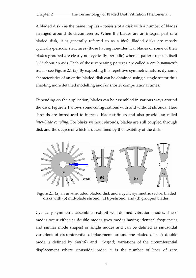
2.1 (a) an un-shrouded bladed disk and a cyclic symmetric sector,
bladed disks with (b) mid-blade shroud, (c) tip-shroud, and (d)
grouped blades.......................................................................................... 9
2.2 (a) Natural frequencies of a 24-bladed bladed disk, and mode
shapes for modes (b) 1F-2 and (c) 2F-2. ............................................... 10
2.3 Clamped-free blade-alone modes : (a) Flexing mode-F, (b) Edgewise
mode-E, (c) Torsional mode-T and (d) Extension mode ................... 11
2.4 Examples of under-platform friction dampers: (a) cottage-roof
damper, (b) thin-plate damper. ............................................................ 13
2.5 A sample Campbell diagram for a 24-blade bladed disk ................. 14
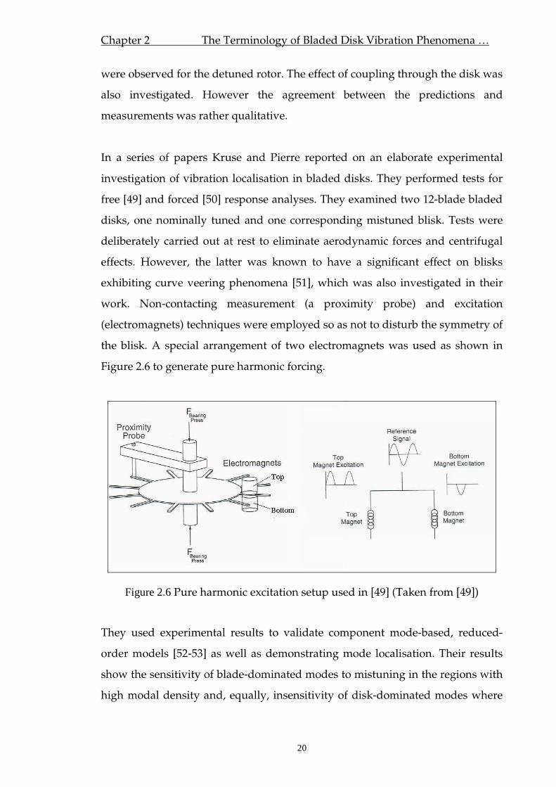
2.6 Pure harmonic excitation setup used in [49] (Taken from [49])....... 20
2.7 (a) A fixed-in-space measurement point diagram, and (b) a typical
vibrometer output................................................................................... 28
2.8 Schematic of the self-tracking system (Taken from [76]) .................. 29
3.1 a) Blisk-1 (as received), and (b) FE model of a cyclic sector ............. 34
3.2 Blade inserts............................................................................................. 34
3.3 Natural frequencies of Blisk-1 at rest (from FE) ................................. 35
3.4 Blisk-1 Campbell diagram (from FE) ................................................... 36
3.5 a) Blisk-2, and (b) FE model of a cyclic sector..................................... 37
3.6 Natural frequencies of Blisk-2 at rest (from FE) ................................. 38
3.7 Blisk-2 Campbell diagram (from FE) ................................................... 38
3.8 Mistuning and damping test rig........................................................... 41
3.9 FE model of the casing and analysis results ....................................... 42
3.10 Shaft FE model and critical speeds for the final design. ................... 43
xiii
3.11 Excitation system .................................................................................... 46
3.12 Working principle of OMETRON VPI Sensor (Adapted from [80])48
3.13 The self-tracking system ........................................................................ 50
3.14 Indexing mechanism .............................................................................. 51
3.15 (a) Conical Circular Scan, (b) Line Scan............................................... 52
3.16 Sources of misalignment (a, b) and its reflection on velocity signal
(c). .............................................................................................................. 53
3.17 (a) The LDV head and (b) the fixed mirror positioning details ....... 54
3.18 LDV alignment technique...................................................................... 55
3.19 (a) No vibration response is measured; (b) true vibration response is
measured.................................................................................................. 55
3.20 Velocity signals with (a), and without (b) dropouts, and the
corresponding frequency spectra, (c) and (d)..................................... 58
3.21 Containment Enclosure (set up for conical LDV scanning, with the
Small-Aperture Cover removed). ......................................................... 59
3.22 Data acquisition layout (—output, —input)....................................... 60
3.23 Process of EO response calculation ...................................................... 64
3.24 Electromagnetic excitation on a stationary blade .............................. 65
3.25 Electromagnet force experienced by a blade (a) large gap and (b)
frequency spectrum. (c) Small gap and (d) frequency spectrum..... 67
3.26 Slow circular scan LDV output............................................................. 68
3.27 Real and imaginary parts of circumferential ODS............................. 69
3.28 (a) Circular scan LDV output, and (b) the frequency spectrum ...... 70
3.29 Comparison of LDV and accelerometer outputs ............................... 71
3.30 Force measurement setup validation................................................... 73
4.1 Damaged areas on Blisk-1 ..................................................................... 76
4.2 Test Arrangement used for measuring individual blade frequencies
................................................................................................................... 77
4.3 Variation of blade-alone natural frequencies ..................................... 78
xiv
4.4 Circular scan spectra and ODSs for the identified first family modes
of Blisk-1................................................................................................... 80
4.5 Blisk-2 impact response spectra............................................................ 82
4.6 ODS comparisons for shifted random mistuning patterns (—1st
pattern, —2nd pattern) ............................................................................ 83
4.7 Lumped parameter bladed disk model ............................................... 86
4.8 Comparison of full FE and discrete Blisk-2 1F frequencies .............. 86
4.9 Blisk-1 tuning simulation....................................................................... 88
4.10 12ND mode’s harmonics variation with increased accuracy in 1F
blade alone modes .................................................................................. 89
4.11 Cases 1 to 4: Split in 1-11 ND modes.................................................... 91
4.12 Mass mistuning corrected through mass and stiffness elements .... 92
4.13 Valid combinations of tuning parameters when (a) one frequency,
and (b) two frequencies are matched................................................... 93
4.14 The comparison of cases given in Table 4.7. ....................................... 95
4.15 Correlation of measured and computed ODSs for 5, 6, 11 and 12D,
1F family modes.................................................................................... 103
4.16 Correlation of applied and identified mistuning patterns - ( )8Sin θ
................................................................................................................. 106
4.17 Correlation between applied and identified mistuning patterns -
Random .................................................................................................. 107
4.18 Identified Blisk-1 mistuning in terms of clamped, sector-alone
frequency deviation.............................................................................. 110
4.19 (a) Correlation between measured and FMM calculated mistuned
modes, (b) Full FE model tuned frequencies vs. FMM ID Advance
estimates................................................................................................. 111
4.20 (a) Correlation of the measured Blisk-1 modes with updated Blisk-1
FE model, (b) measured and computed Blisk-1 frequencies for 1F
modes (8-24)........................................................................................... 113
4.21 Updated Campbell diagram with identified fine and coarse speed
step regions for Blisk-2......................................................................... 115

xv
4.22 Measurement plan for a particular EO response curve .................. 117
4.23 Regular and random mistuning patterns to be used in rotating
(Blisk-2 tests).......................................................................................... 119
4.24 Computed Campbell diagram for ( )8Sin θ⋅ mistuned Blisk-2, blade
18 (red spots indicate resonances). ..................................................... 120
4.25 Normalised amplitude spectrum of the first 12 spatial harmonics for
the first 24 Blisk 2 modes, with applied ( )8Sin θ⋅ mistuning. ....... 121
4.26 Computed Campbell diagram for random mistuned Blisk-2, blade
20 ............................................................................................................. 124
4.27 Normalised amplitude spectrum of the first 12 spatial harmonics for
the first 24 Blisk 2 modes, with applied random mistuning. ......... 124
4.28 (a) Simple FE model used in damper design, (b) free body diagram
of a damper............................................................................................ 127
4.29 Designed damper and its integration ................................................ 128
4.30 Computed Campbell diagram for updated Blisk-1 FE model
including inherent mistuning, 4-24 EOs............................................ 129
5.1 Mistuning patterns applied to stationary Blisk-2............................. 135
5.2 Split in 1F family double modes due to applied mistuning patterns
................................................................................................................. 135
5.3 Comparison of ODSs for stationary Blisk-2 with applied random
mistuning. .............................................................................................. 137
5.4 (a) Original and shifted mistuning patterns, (b) comparison of 10-
EO response curves for both patterns – shaded circles indicate
corresponding measurement locations.............................................. 138
5.5 Comparison of 6EO excitation response using mode shapes
calculated at different speeds.............................................................. 140
5.6 A typical train of magnet pulses applied to Blisk-2 @ 120 rev/min.
................................................................................................................. 141
5.7 Harmonics of a magnet pulse and its reconstruction through these
harmonics............................................................................................... 142

xvi
5.8 Comparison of experimentally and numerically obtained
resonances.............................................................................................. 143
5.9 (a) Amplitude, and (b) phase plots of 6EO forced response on blade
#1. ............................................................................................................ 145
5.10 Comparison of response measurements for 6, 8 and 12 EO
excitations (η =0.0001 in predictions)................................................. 146
5.11 Comparison of 6EO response amplitudes away from 6EO-6ND
resonance and measured inter-blade phase angles. ........................ 147
5.12 (a) mistuning masses attached to Blisk-2 (picture shows random
mistuning pattern), (b) sector model used in MISTRES.................. 148
5.13 (a) Predicted and (b) measured z-mod plots for Blisk-2 with applied
8S θ mistuning ...................................................................................... 150
5.14 Response of Blisk-2 with 8S θ mistuning to 6EO excitation - all
blade measurements............................................................................. 151
5.15 Blisk-2 with 8S θ mistuning pattern: Comparison of individual
blade responses to 6EO excitation...................................................... 153
5.16 Close-up of covered resonance groups Measured and predicted
amplitude curves for blade #1............................................................. 154
5.17 Comparison of blade-to-blade amplitude variation at (a) point A,
and (b) point B shown in 5.16. ............................................................ 155
5.18 Predicted and measured z-mod plots for Blisk-2 with applied
random mistuning ................................................................................ 156
5.19 Blisk-2 with random mistuning pattern: Comparison of individual
blade responses to 10E excitation. —Measured, —Predicted. (x-axes:
Frequency (Hz), y-axes: Amplitude (dB) – re 100 mm/s)...................... 158
5.20 Amp. and phase measurements for blades (a) 8, (b) 22, and (c) 23.
................................................................................................................. 160
5.21 Response of blade 2 to 9, 10 and 11 EO excitations.......................... 160
5.22 Response of Blade 21 to 10EO excitation........................................... 162
5.23 Comparison of blade-to-blade tip amplitude variations at various
resonances excited by 10EO excitation. ............................................. 164

xvii
5.24 Inter-blade phase angles corresponding to amplitude plots given in
Figure 5.23 (a) and (b). ......................................................................... 164
5.25 Blisk-2 with 8S θ mistuning pattern: Comparison of individual
blade responses to 6E excitation. —Measured, —Predicted. (x-axes:
Frequency (Hz), y-axes: Amplitude (dB) – re 100 mm/s)...................... 170
6.1 Different stages in DOF reduction and formation of non-linear
equations (Adapted from [40]) ........................................................... 169
6.2 Introduction of mistuning in Blisk-1.................................................. 170
6.3 Comparison of different ways of mistuning modelling, (a) % split in
ND mode pairs ...................................................................................... 171
6.4 Introduction of mistuning through different number of nodes..... 172
6.5 A typical magnet force signal applied to Blisk-1.............................. 172
6.6. Variation of peak magnet force applied to blades of Blisk-1.......... 173
6.7 (a) Applied force distributions, (b) forced response of blade 1, and
(c) maximum blade-tip forced response amplitude comparison for
mistuned Blisk-1. .................................................................................. 176
6.8 Statistical variation of maximum 9EO response amplitude due to
excitation errors on the (a) tuned and (b) mistuned Blisk-1 FE
model. ..................................................................................................... 177
6.9 (a) Error in mistuning pattern, (b) Maximum forced response
variation of a discrete bladed disk model due to errors in mistuning
pattern .................................................................................................... 178
6.10 (a) Computed and (b) measured interference diagrams on blade 1 of
the undamped Blisk-1 .......................................................................... 180
6.11 Response of blade 1 to EO excitations 5, 6, 7, and 8......................... 181
6.12 Undamped Blisk-1: Comparison of individual blade responses to
9EO excitation. —Measured, —Predicted. (x-axes: Frequency (Hz), y-
axes: Amplitude (dB) – re 100 mm/s)..................................................... 183
6.13 Measured and predicted ODSs for (a) 5, (b) 6, and (c) 9ND modes
excited by 5, 6, and 9EOs respectively. .............................................. 185

xviii
6.14 (a) a C-R damper, and (b) its installation in Blisk-1......................... 186
6.15 FE modelling of friction interfaces ..................................................... 188
6.16 (a) Undamped and (b) Steel C-R damper fitted Blisk-1 z-mod plots
................................................................................................................. 189
6.17 Ti C-R damper fitted Blisk-1 excited with 2 magnets...................... 190
6.18 Blisk-1 –Response of blade 1 to (a) 19EO, and (b) 17EO excitations
................................................................................................................. 192
6.19 Ti C-R damper fitted Blisk-1 excited by a single magnet................ 193
6.20. Response of Blisk-1 fitted with Ti C-R dampers excited by (a) 19, (b)
18, and (c) 17 EOs.................................................................................. 194
6.21 (a) Blade 1 tip response @ 19EO-5ND resonance, (b) a jammed
damper, and (c) a damper surface after shutting down. ................ 195
6.22 Responses of first 4 blades to EOs 19, 18 and 17 after the first
cleaning of dampers and inserts......................................................... 197
6.23 (a) 19EO response of all blades after 4th and last installation of
dampers; (b) maximum amplitude, and (c) inter-blade phase angle
variation. ................................................................................................ 198
6.24 (a) Response of blade 1 to 19EO excitation for all installations, and
time histories @ 884 rev min for (b) installation 1 and (c) installation
4. .............................................................................................................. 199
6.25 (a) Response of first 5 blades to EO20 excitation, (b) blade-to-blade
amplitude variation, and (c) inter-blade phase angles @ the
resonance speed. ................................................................................... 200
6.26 (a) variation of force signal amplitude with rotational speed, (b)
response of blade 1 to EO20 excitation at various blade-magnet
distances ................................................................................................. 201
6.27 Comparison of measured and computed damped Blisk-1 response
on blade # 1 to 19EO excitation; µ =0.45 ........................................... 203
6.28 Comparison of measured and computed damped Blisk-1 response
on blade # 1 to (a) 18, and (b) 17 EO excitations; µ =0.45. .............. 206

xix
6.29 Comparison of measured and computed damped Blisk-1 response
on blade # 1 to (a) 18, and (b) 19 EO excitations; µ =0.6. ................ 206

xx
List of tables
3.1 Separation of Blisk-1 first family modes (from FE)............................ 35
3.2 Separation of Blisk-2 1F family modes (from FE) .............................. 38
3.3 Comparison of speed values on motor and rotor side (all speed
values in rev/min).................................................................................. 44
4.1 Statistics of blade-alone natural frequencies....................................... 78
4.2 1F ND modes of Blisk-1 before and after tuning................................ 80
4.3 Measured 1F Blisk-2 frequencies. ......................................................... 82
4.4 Random mistuning patterns ................................................................. 83
4.5 Correlation of randomly mistuned Blisk-2 ODSs .............................. 84
4.6 Mistuning/tuning test configuration................................................... 90
4.7 Mistuning/tuning test configuration................................................... 94
4.8 Initial correlation of measured and computed Blisk-2 1F frequencies
(all frequencies in Hz) .......................................................................... 101
4.9 Blisk-2, 5-12ND 1F, 1E, 2F and 3F family natural frequencies,
measured and updated (all frequencies in Hz) ................................ 103
4.10 Correlation between initial FE and measured frequencies (--
Frequencies used in IES method, --: modes used in mistuning
identification) ........................................................................................ 108
4.11 Blisk-1 FE frequencies after updating via IES method.................... 109
5.1 Natural frequencies of the 8S θ mistuned blisk modes, measured
and predicted......................................................................................... 149
5.2 1F family natural frequencies of the randomly mistuned Blisk-2 at
rest........................................................................................................... 155
6.1 Blade inserts and C-R damper masses (*: Total includes 4 retaining
screws, each weighing 0.13g) .............................................................. 187

Chapter 1 Introduction
1
CHAPTER 1
INTRODUCTION
1.1 Overview
There are a few components, such as turbomachinery bladed disks, that have
drawn a great deal of attention from researchers in the field of structural
dynamics for more than half a century. Given their extensive use and the crucial
role they play in applications, such as aeroplane jet engines, this is only
understandable. Figure 1.1 shows pictures of a jet engine cross-section and some
bladed disks used in real applications.
Figure 1.1 (a) Cross-section of Pratt & Whitney JT9D-7J engine powering Boeing 747, (b) Typical bladed disks (from www.mtu.de)
Bladed disk vibration amplitudes are known to be seriously amplified and
varied from blade to blade due to scatter in blade geometry or due to variations
in material properties. The phenomenon of having non-identical blades due to
these kinds of variation is called mistuning and the distribution of the variation
across the bladed disk is called a mistuning pattern. This pattern is generally

Chapter 1 Introduction
2
random and unknown to the manufacturer or user. Since mistuning can lead to
forced response amplitudes which are much grater than those predicted for a
tuned assembly (i.e. one having identical blades), additional dissipation
elements (i.e. dampers) are sometimes integrated into the bladed disk assemblies
in order to control the vibration amplitudes. Often so-called friction dampers are
used for this purpose. As the name implies, energy is dissipated via rubbing of
the damper and blade surfaces against each other.
1.2. Definition of problem
Due to the crucial role they play during the operation of gas turbine engines,
blades and bladed disks require special attention and very careful design. As so
much is dependent on the reliability of these components, manufacturers are
always keen to be on the safe side of their products’ limitations. This, however,
generally leads to an over-designed and therefore inefficient product.
In order to optimise the design of bladed disks, many research studies have
addressed the problems associated with the vibration behaviour of these
components. The engine manufacturer’s main concern is to control the resonant
response levels of the blades, and therefore the peak resonant stresses in the
engine blading. This is one of the major problems in the design of bladed disks
since the vibration response of gas turbine blades that occur in practice is very
sensitive to mistuning. When the inherent dissipation mechanisms are not
sufficient (i.e. when the damping present is low), blade vibration amplitudes can
reach higher than the acceptable levels. To avoid the risk of catastrophic failure
due to such large amplitude vibrations, inter-blade friction dampers are often
incorporated into the bladed disks. However, before implementing such friction
dampers, the damping level needed to control the vibration should be predicted
and the dampers should be designed accordingly. Therefore, the primary
concern for many studies has been to seek an understanding of (i) what the least
and the most severe consequences of mistuning are, and (ii) how they can be

Chapter 1 Introduction
3
controlled. These concerns have been the subject of several studies carried out at
Imperial College and elsewhere in the past. As a result, several Finite Element
(FE) model-based computer codes have been developed. With the aid of these
codes, it is now possible to predict the response of a bladed disk for any
mistuning pattern with integrated friction dampers. It is also possible to
determine the worst mistuning pattern which leads to extreme blade vibration
amplitudes. Nevertheless, developing codes – no matter how complicated - does
not necessarily guarantee their accuracy and predictability. Since these codes are
not yet validated against real structures and the realistic conditions they
simulate, manufacturers are reluctant to incorporate them in their production
chain.
In order to make these codes effective in the design and production of bladed
disks, an extensive validation study is essential. This study must aim to identify
possible sources of mismatch between the real and simulated data and to guide
the codes in any necessary corrections to produce acceptable and reliable
estimates.
In general, discrepancies between computer model predictions and actual
system responses are due either, to inaccurate modelling of some aspects of the
dynamics of the system, or to not modelling them at all. When there is a
disagreement between the experimental results and numerical simulations,
generally the numerical models are believed to be inefficient or not capable of
handling the problem. However, this may not be the case all the time. Given the
advanced state of the FE modelling, it can be said that mass and stiffness
distributions of the components being analysed can be estimated fairly
accurately. However the mistuning distribution and the incorporated damping
model are, in general, much less certain and are often responsible for the poor
predictions that are often obtained. For example, depending on whether the
mistuning is due to the dimensional variations or variations in the material
properties, the numerical model will be different and so will the predicted

Chapter 1 Introduction
4
behaviour. Similarly, assumptions inevitably involved in the damping model
used may well describe a damping mechanism which is different from the one
which exists in the real structure.
The ultimate way of making sure that these phenomena are modelled correctly
is to check the numerical predictions against experimental measurements.
However, validating a model which is used to predict the mistuned vibration
response of a bladed disk on a real gas turbine engine would be extremely
difficult. This is because in the engine there are several other components apart
from the bladed disk itself, which affect the vibration response of the blades and
yet remain unconsidered in the model. Even the bladed disk assembly alone
may be so complicated (i.e. due to joints, etc.) that it cannot be handled properly
by the model. Moreover, in most cases there will not be enough room to
incorporate a measurement system to acquire the necessary data in a real engine
measurement. As the numerical model is only as accurate as the input data,
these measurements should be made on a carefully-constructed experimental
setup, which exhibit only the phenomena under investigation.
Once the numerical models are demonstrated to be accurate representations of
the experimental test cases, and the assumptions involved in the modelling are
justified, they can be confidently used to predict the vibration responses of real
bladed disks and to optimise their design.
1.3. Objectives of the study
The main objectives of the presented work are to design and conduct tests to
validate
• the tuned and mistuned vibration response predictions of integral
turbomachinery bladed disks (blisks) and to do so with the application of
various mistuning patterns both statically and under rotation, and
Chapter 1 Introduction
5
• the undamped and friction damper damped blade vibration forced
response predictions under rotation.
Additional goals in fulfilment of abovementioned objectives are:
• To devise and commission a vibration measurement technique which
comprises non-contacting measurement (based on the LDV) and
excitation (magnetic) techniques, and functions under rotation and
independent of rotational speed
• To build a well-controlled rig and carefully-designed test pieces which
only exhibit the phenomena considered in the predictions
• To study bladed disk tuning through individual blade frequencies and
the translation of frequency mistuning into physical mistuning
• To study the effects of variations in Engine Order (EO) force amplitudes,
applied on individual blades, on vibration response.
1.4 Overview of the thesis
This thesis presents experimental work comprising systematic and well-planned
tests in an attempt to validate the predictions of mistuned (i.e. linear) and
friction damped (i.e. non-linear) forced response predictions of turbomachinery
bladed disks. The presentation of the work is structured in the following way:
Chapter 2, starting with the introduction of basic definitions and terminology
related to bladed disks, summarises the relevant literature on validation of
vibration response predictions, and mistuned and damped bladed disk studies.
The focus is on experimental studies. Nonetheless, the main areas of research on
mistuned and/or damped bladed disks are also outlined. Finally, a review of the
use of Laser Doppler Velocimeter (LDV) transducers on rotating bladed disks is
presented.
Chapter 3 concentrates on the design and instrumentation aspects of test pieces
and the rig used in measurements. The objectives of the intended rig, and the
Chapter 1 Introduction
6
desired and achieved characteristics of the test pieces are presented. Details of
the excitation and measurement techniques are given and the hardware and
software employed in measurements are introduced. The processing of LDV
vibration output to obtain frequency forced response and Operating Deflection
Shapes (ODSs) is presented. Advantages and limitations of LDV transducers are
also discussed in this chapter
Chapter 4 presents the attempts made at maximising the efficiency of the
measurements through careful test planning based on properly updated test
piece FE models. The actual characteristics of the blisks are identified and
improvement to their symmetry (i.e. tuning) is sought when necessary. The
sensitivity of the blisk dynamic properties to various ways of tuning is
investigated through a discrete bladed disk model. The blisk models are
updated, based on the measured characteristics using the employed updating
methods. Using these updated models, a comprehensive test plan is designed.
Validation of undamped tuned and mistuned bladed disk forced response
predictions, both at rest and rotating, are given in Chapter 5. The prediction tool
used in computations is presented. The results obtained from rotating tuned,
and sinusoidally and randomly mistuned blisk are presented. Obtained
predictions are correlated to these results and the degree of success and the
sources of possible deviations are discussed.
Chapter 6 is devoted to the assessment of friction damped bladed disk forced
response measurements and predictions. However, first the undamped blisk
response is considered to assess the degree of correlation in the absence of non-
linearity. The non-linear forced response prediction tool is introduced. The
effects of different ways of modelling frequency mistuning in terms of physical
mistuning on forced response are analysed. Also in this chapter, the
consequences of EO excitation errors are discussed and the effects are shown in
the Blisk-1 FE model.

Chapter 1 Introduction
7
The overall conclusions are summarised in Chapter 7. The degree of success in
achieving the task undertaken is discussed and some recommendations in the
furthering of the work performed here are presented.

Chapter 2 The Terminology of Bladed Disk Vibration Phenomena …
8
CHAPTER 2
The TERMINOLOGY of BLADED
DISK VIBRATION PHENOMENA
and LITERATURE SURVEY
2.1 Overview
In this chapter the relevant literature on mistuned and damped bladed disk
vibration studies will be reviewed. The chapter will be divided into three parts.
In the first part basic definitions and terminology related to bladed disk
vibration phenomena will be given. Then, in the second part, relevant studies
carried out on bladed disk vibration will be presented. The focus will be on the
experimental studies although the main areas of research on mistuned and/or
damped bladed disks will also be outlined. Finally in the last part, a review of
the use of Laser Doppler Velocimeter (LDV) transducers on rotating
components, such as bladed disks, will be presented.
2.2 Basic definitions and terminology
Over the years, bladed disks, especially those used in aircraft jet engines have
been the subject matter of a wide range of studies. Given the environment they
work in, and the role they play on the safety of aircraft, this is only
understandable. As a result a highly specific terminology regarding these
structures is generated. A thorough explanation of mentioned terminology can
be found in several references such as [1]. However, a brief summary of certain
terms and definitions is thought useful before the literature on the subject is
reviewed. The mentioned reference is made use of in preparation of following.
Chapter 2 The Terminology of Bladed Disk Vibration Phenomena …
9
A bladed disk - as the name implies - consists of a disk with a number of blades
arranged around its circumference. When the blades are an integral part of a
bladed disk, it is generally referred to as a blisk. Bladed disks are mostly
cyclically-periodic structures (those having non-identical blades or some of their
blades grouped are clearly not cyclically-periodic) where a pattern repeats itself
360° about an axis. Each of these repeating patterns are called a cyclic-symmetric
sector - see Figure 2.1 (a). By exploiting this repetitive symmetric nature, dynamic
characteristics of an entire bladed disk can be obtained using a single sector thus
enabling more detailed modelling and/or shorter computational times.
Depending on the application, blades can be assembled in various ways around
the disk. Figure 2.1 shows some configurations with and without shrouds. Here
shrouds are introduced to increase blade stiffness and also provide so called
inter-blade coupling. For blisks without shrouds, blades are still coupled through
disk and the degree of which is determined by the flexibility of the disk.
Figure 2.1 (a) an un-shrouded bladed disk and a cyclic symmetric sector, bladed disks with (b) mid-blade shroud, (c) tip-shroud, and (d) grouped blades.
Cyclically symmetric assemblies exhibit well-defined vibration modes. These
modes occur either as double modes (two modes having identical frequencies
and similar mode shapes) or single modes and can be defined as sinusoidal
variations of circumferential displacements around the bladed disk. A double
mode is defined by )( θnSin and )( θnCos variations of the circumferential
displacement where sinusoidal order n is the number of lines of zero

Chapter 2 The Terminology of Bladed Disk Vibration Phenomena …
10
displacement across the assembly or, as is generally know, the number of nodal
diameters and θ is the angular separation of two adjacent blades. Note that in
case of bladed disks, patterns formed by zero displacements are slightly more
complicated than simple lines due to finite number of blades – see Figure 2.2 (b).
For a bladed disk with N blades, the number of nodal lines is limited to 2/N if
N is even and 2/)1( −N if N is odd. However, for a continuous disk when its
circumferential motion is not described only by some discreet points, nodal
diameters higher than N /2 are possible. Here the modes with 0=n and
2/Nn = (only when N is even) are single modes in which all the blades
experience the same amplitude, in phase when 0=n and out-of-phase with
neighbouring blades when 2/Nn = . All the other modes occur in pairs. For a
given natural frequency, nω , for which a double mode exists, the overall mode
shape or rather Operating Deflection Shape (ODS) is a combination of both of the
modes and is in the form of )( ϕθ +nCos , where ϕ is a phase angle. The
implication of this is that, a natural frequency can be associated with a particular
nodal diameter, n , regardless of radial section’s displacement shape. However,
for a perfectly tuned bladed disk the angular orientation of these nodal diameter
lines is not fixed and they can be anywhere on the structure. Figure 2.2 (a) shows
the first 72 natural frequencies of a bladed disk with 24 blades plotted against
the nodal diameter numbers with which they are associated.
0 1 2 3 4 5 6 7 8 9 10 11 120
500
1000
1500
2000
2500
3000
3500
4000
4500
5000
Nodal diameters
Fre
quen
cy (H
z)
1F
1E
2F
1T
3F
2E
A
1F-2
2F-2
B
(a)
Figure 2.2 (a) Natural frequencies of a 24-bladed bladed disk, and mode shapes for modes (b) 1F-2 and (c) 2F-2.

Chapter 2 The Terminology of Bladed Disk Vibration Phenomena …
11
It is seen from Figure 2.2 (a) that the natural frequencies are grouped into several
distinct families. As the number of nodal diameters, n , increases the natural
frequencies in each family asymptotically approach one of the clamped, blade-
alone frequencies (i.e., the natural frequencies of a blade when it is grounded at
the boundary where it joins the disk). These families of modes are generally
described by the mode shape of the blade mode they converge to. Some of these
blade-alone mode shapes are shown in Figure 2.3 for a simple blade model. Note
that these mode shapes are usually more complicated (generally a combination
of given basic shapes) for real blades with complex geometries and a
classification of this kind may not strictly apply.
Figure 2.3 Clamped-free blade-alone modes : (a) Flexing mode-F, (b) Edgewise mode-E, (c) Torsional mode-T and (d) Extension mode
When the mode shapes corresponding to natural frequencies associated with the
same nodal diameter number, such as those enclosed in region A in Figure 2.2
(a), are investigated, it is observed that, depending on the family of modes they
are in, they may possess nodal points in the radial direction in addition to the
nodal diameter lines they have in a circumferential direction. These points form

Chapter 2 The Terminology of Bladed Disk Vibration Phenomena …
12
circles around the bladed disk and therefore are called nodal circles. See Figure
2.2 (c) for 2 ND mode of 2nd flex (2F) family for a bladed disk with 24 blades.
A bladed disk is said to be tuned when all its sectors are identical. However, in
reality, making sure that all the sectors are identical is quite difficult. Inevitable
variations due to manufacturing tolerances, material variations, damage, or
operational wear cause the symmetry to be disturbed. A bladed disk with these
variations is said to be mistuned or detuned and some of its forced response
amplitudes are known to be amplified considerably as a result of these
variations. As a result, a substantial research effort has been devoted to
understanding this problem. It is now well known that mistuning causes mode
localisation in which vibration energy of a mode is confined to only a blade or a
few blades, resulting in large forced response amplitude magnifications
compared to those of a reference tuned case. Moreover, the sensitivity of the
forced response to mistuning is shown to be significantly affected in the
presence of so called frequency veering or curve veering [9] which refers to the
interaction between different families of modes and manifests itself by a veering
in the natural frequencies when they are plotted against the number of nodal
diameters. A curve veering region is indicated by region B in Figure 2.2 (a). As
the resulting large vibration amplitudes, in turn, cause high cycle fatigue (HCF)
problems, they need to be eliminated. One way of doing this is to specify very
strict tolerances in manufacture to make sure that these variations are minimal.
However, even if it was possible to make a perfectly tuned bladed disk,
maintaining this status throughout the operational life is almost impossible due
to irregular wear patterns. Besides, tight tolerances will eventually increase
production costs. Another way of tackling this problem is to employ additional
energy dissipation elements (i.e., in addition to structural damping which is
generally quite low and aerodynamic damping). For this purpose friction
dampers of various types are most commonly used. These dampers are placed
between neighbouring blades and energy is dissipated by interfacial rubbing of

Chapter 2 The Terminology of Bladed Disk Vibration Phenomena …
13
the blade-damper contact surfaces due to relative motion of the adjacent blades.
Some friction damper configurations are given in Figure 2.4.
Figure 2.4 Examples of under-platform friction dampers: (a) cottage-roof damper, (b) thin-plate damper.
In addition, some novel techniques, such as those which seek to reduce the
sensitivity of the bladed disk to mistuning by intentionally mistuning it in a
certain way (based on the fact that after a certain degree, additional mistuning
reduces forced response amplitudes, [43]), are also being considered to reduce
the sensitivity to mistuning hence reduce the forced response amplitudes.
Bladed disks are mostly subjected to a special form of excitation known as engine
order (EO) excitation where the bladed assembly rotates past a static pressure or
force field. The blades of an assembly facing such an excitation are excited in a
way which is periodic in time and varies only in phase from blade to blade. For a
steady force/pressure field with a sinusoidal variation, the force experienced by
a particular blade, j at a given time t and for a rotational speed Ω is given by
[1] )( φjtkCosFf j +Ω= . Where F is the amplitude of the force and k is the
engine order, or the number of excitation cycles a blade experiences in a full
rotation of bladed disk (i.e., number of stationary excitation sources equally
spaced in the flow field). Inter blade phase angle, φ in this case is given by
Nk /2πφ = where N is the number of blades. The implication of this is that, an
EO excitation of kth order can only excite those modes with k nodal diameters
for a perfectly tuned bladed disk or modes having k diameter components in

Chapter 2 The Terminology of Bladed Disk Vibration Phenomena …
14
their mode shapes in the case of a mistuned bladed disk. EO forced response
characteristics are best demonstrated on a Campbell or interference diagram
where frequencies are plotted against rotational speed. A sample Campbell
diagram constructed using a lumped parameter model of a perfectly tuned 24-
bladed bladed disk is given in Figure 2.5 (note that not all the order lines are
plotted for clarity).
500 1000 1500 2000 2500 3000120
140
160
180
200
220
240
260
280
300
Rotor Speed (rev/min)
Fre
quen
cy (
Hz)
1ND
2ND
3ND
4ND
5ND 6ND
6E
5E
4E
7E 8E 9E 10E 11E 12E 24E 36E
Figure 2.5 A sample Campbell diagram for a 24-blade bladed disk
Here the 3rd dimension, as shown by the sample blue curve, is the vibration
amplitude. Although a particular EO line crosses many frequency lines, a
resonance occurs only when the kth EO line intersects a natural frequency line
of a k -ND mode and this is indicated by a solid circle on the diagram. No
resonant response is produced for all the other crossings since for a resonance to
occur the shapes as well as the frequencies of the force and structural mode
should match. Note that due to spatial aliasing k ND modes will be excited by
k , )( kN + , )( kN − etc. EOs and this is clearly observed from the given
Campbell diagram.

Chapter 2 The Terminology of Bladed Disk Vibration Phenomena …
15
2.3 Literature survey on bladed disk vibration
2.3.1 Classification of bladed disk research areas
A huge amount of research has been generated in the area of damped and
mistuned bladed disk vibration predictions and a review of all the relevant
literature is beyond the scope of this study. The interested reader is directed to
major survey papers such as [2-4] and the references given therein. However, at
this stage it is worth giving a classification of the research in these areas. Some of
the recent references are given below. The research on mistuned bladed disks is
mainly collected under a few groups;
(i) identification of the most sensitive parameters influencing mistuning
such as blade-disk coupling, rotational speed, modal density,
mistuning amplitude, frequency veering, damping variation etc. [5-9,
41],
(ii) reduction of model size to have computationally efficient yet
representative models to carry out parametric studies as well as
reducing prediction times [10-15],
(iii) probabilistic analysis of mistuned bladed disks to determine forced
response statistics [6,16, 17],
(iv) maximum/minimum response amplitude predictions using
numerical/analytical [20], optimisation [18,19] or statistical techniques
[21],
(v) use of intentional mistuning to minimise the adverse effects of
inherent random mistuning [22-24],
(vi) mistuning identification based on experimental data to assess the
suitability of the bladed disk for operational use [25-29], and
(vii) experimental investigations aiming at validation of models developed
for above-mentioned phenomena [44, 46, 49-50, 54-59]
Research on last two items is reviewed in separate sections (2.3.2, 2.3.3.1) below
due to their relevance to this study.

Chapter 2 The Terminology of Bladed Disk Vibration Phenomena …
16
A similar breakdown of research areas can be given for damped bladed disk
studies as well. There are three main damping mechanisms concerning bladed
disk analyses; inherent material damping, aerodynamic damping and external
mechanical damping. In the following list, the studies concentrated on external
mechanical damping, friction in particular, introduced at the contact interfaces
are mentioned. Most of the research in this area is directed mainly towards
(i) the identification (mainly experimental) of friction contact parameters
such as coefficient of friction and contact stiffness, to provide the
prediction tools with realistic data [30-32],
(ii) the development of realistic friction damping and contact models or
modelling of friction/contact interfaces [33-38],
(iii) non-linear forced response predictions of assemblies fitted with
friction dampers [39-40], and
Again, for more references, a survey paper such as [42] and references given in
the references mentioned above can be consulted. Similarly, some of the
experimental works in these areas are reviewed in section 2.3.3.2. Detailed
explanations of prediction tools [14, 39-40] used in this study can also be found
in chapters 5 and 6.
2.3.2 Identification of individual blade variation
When predictions of a specific numerical code are to be compared with
experimental data collected, the degree of correlation depends not only on the
prediction tool’s capabilities to capture the dynamic characteristics of the
structure but also on how well the structure is described to the prediction tool.
Mistuning response prediction tools are no exception to this. When validating
these codes, special attention should be given to identification of the true
mistuning parameters. Moreover, inherent mistuning identification may benefit
the research efforts seeking to reduce the sensitivity to mistuning by introducing
suitable intentional mistuning. Therefore it is thought appropriate to report
some of the proposed methods on mistuning identification.

Chapter 2 The Terminology of Bladed Disk Vibration Phenomena …
17
Mignolet et. al. and Rivas-Guerra et. al. [25-26] focused on estimations of blade-
to-blade variations of masses and stiffnesses in a two part investigation. They
used measured lowest frequencies of the isolated blades to recover variations in
mass and stiffness properties. Two methods are presented. The first one assumes
the mass matrix’s variation to be negligible and associates mistuning to stiffness
variations only. However this way it is found that significant errors are
introduced in estimations of forced response. In the second method, maximum
likelihood (ML) strategy is employed in which a simple Gaussian distribution of
mass and stiffness matrices is assumed and all the structural parameters are
estimated. However, this technique is only applicable to bladed disks with
separate blades and it is assumed that individual blades behave in the same way
when they are assembled.
A mistuning identification method which predicts individual blade stiffness
variations from measurements on an entire bladed disk is given by Judge et. al.
[27]. This method, unlike the above, can be applied to blisks. A highly reduced
order model [10] is used in which blade modal stiffnesses are isolated. The
variations of these stiffnesses then are calculated based on measurement data to
assess the degree of deviation from a tuned reference. The capabilities of the
method are demonstrated on an experimental bladed disk. Although the
variation of intentional mistuning imposed on experimental test piece is
predicted reasonably well, significant deviations are observed in quantification
of mistuning.
Feiner and Griffin proposed a completely experimental mistuning identification
method [28-29] which requires only a set of measured bladed disk modes and
works out mistuning as a sector-to-sector frequency deviation relative to
corresponding tuned reference. Unlike the method proposed by Judge et. al. it
only works for an isolated family of modes. However, the model reduction
methodology involved is less complicated and requires less analytically
Chapter 2 The Terminology of Bladed Disk Vibration Phenomena …
18
generated input data. Their method is based on the so called Fundamental
Mistuning Model (FMM) [13] in which a highly-reduced 1 DOF per sector model
of a bladed disk is used to predict the vibratory response in an isolated family of
modes. The effectiveness of the method is experimentally demonstrated on a test
specimen. Very good agreement between applied, predicted and identified
mistuning, both in terms of shape and magnitude is obtained. However the fact
that it can only be applied to an isolated family of modes and uses a rather
simple sector model limits its applicability wherever these assumptions are not
valid. This method is partly used in mistuning identification of test pieces
investigated in the presented study. For a more detailed explanation on the
method refer to Chapter 4.
2.3.3 Experimental studies on bladed disks
Compared with the large number of theoretical studies on mistuning and
damping in bladed disks, experimental investigations of these structures,
particularly under rotation, for the validation of predictions of the mentioned
phenomena are rather rare. This is mainly because of the difficulties involved in
the required measurement and excitation techniques as well as precise and well-
controlled test setups. In the case of mistuning the task is further complicated by
the fact that the test application is expected to capture the variations in response
due to small changes in the test structure. On the other hand, when damping
elements like friction dampers are present, the non-linear nature of the structure
makes testing even more challenging. In particular, when mistuning is
investigated, the use of conventional excitation and response measurement
techniques which require placement of transducers and exciters on the test
structure, can modify original mistuning significantly.
In the following sections, experimental studies reported in the area of bladed
disks will be reviewed. This review is divided into two areas namely, (i)
mistuning studies, and (ii) damping studies.

Chapter 2 The Terminology of Bladed Disk Vibration Phenomena …
19
2.3.3.1 Mistuning studies
One of the earliest thorough experimental investigations of mistuned bladed
disks was carried out by Ewins in 1970s [43-45]. Tests were conducted on an
integral bladed disk (blisk) having 24 blades. Inherent mistuning in the blisk was
accounted for by the addition of small bolts and washers to the blade tips to get
a tuned reference for mistuning analysis. Intentional mistuning was introduced
the same way on top of this reference case. In order to eliminate the effects of
aerodynamic forces tests were carried out in an evacuated chamber.
Measurements here were taken on a rotating blisk which allowed the inclusion
of centrifugal effects. Strain gauges were used to measure blade tip responses
and excitation was performed via carefully arranged air jets close to blade tips.
The number of jets could be adjusted to obtain the desired EO excitation.
However the fact that air jets were used to excite the system subsequently led to
deterioration of the vacuum and introduced variability in damping, and also
brought up significant variations in force amplitudes. Nevertheless, satisfactory
qualitative agreement between theory and measurements is demonstrated for
several mistuning patterns thus validating the theory. Ewins observed, through
measurements and was also able to simulate through predictions, the formation
of rather complex, irregular modes in which some blades experienced much
higher vibration amplitudes and no longer could be described by nodal diameter
shapes. These modes were later identified as localised modes and the
mechanism behind them was explained by Wei and Pierre [47-48].
Fabunmi [46] reported an experimental study in early 80s where a 23-bladed
axial compressor rotor was used. Experiments were carried out on the stationary
rotor to acquire modal data which were subsequently used with a semi-
empirical method to calculate vibration response of the rotor. Here the blades
were driven by piezoelectric actuators placed at the blade roots, and response
was measured using a time-averaged holographic technique. The phase and
amplitude for each actuator was controlled independently to generate EO-like
excitations. Amplitude variations and departures from the regular ND modes
Chapter 2 The Terminology of Bladed Disk Vibration Phenomena …
20
were observed for the detuned rotor. The effect of coupling through the disk was
also investigated. However the agreement between the predictions and
measurements was rather qualitative.
In a series of papers Kruse and Pierre reported on an elaborate experimental
investigation of vibration localisation in bladed disks. They performed tests for
free [49] and forced [50] response analyses. They examined two 12-blade bladed
disks, one nominally tuned and one corresponding mistuned blisk. Tests were
deliberately carried out at rest to eliminate aerodynamic forces and centrifugal
effects. However, the latter was known to have a significant effect on blisks
exhibiting curve veering phenomena [51], which was also investigated in their
work. Non-contacting measurement (a proximity probe) and excitation
(electromagnets) techniques were employed so as not to disturb the symmetry of
the blisk. A special arrangement of two electromagnets was used as shown in
Figure 2.6 to generate pure harmonic forcing.
Figure 2.6 Pure harmonic excitation setup used in [49] (Taken from [49])
They used experimental results to validate component mode-based, reduced-
order models [52-53] as well as demonstrating mode localisation. Their results
show the sensitivity of blade-dominated modes to mistuning in the regions with
high modal density and, equally, insensitivity of disk-dominated modes where

Chapter 2 The Terminology of Bladed Disk Vibration Phenomena …
21
modes are reasonably separated. In-plane modes, in particular, are found to be
very sensitive to mistuning due to their high modal density. Though the
qualitative distortion to vibration modes due to mistuning was captured by their
reduced order model, reduction was achieved at the expense of loss of accuracy
in quantification of these changes.
In a later study Kruse and Pierre [50] abandoned the use of electromagnets due
to collapse of magnetic fields at high frequencies and replaced them with piezo-
electrical actuators which in turn contributed to the mistuning of the blisks.
Forced response measurements and corresponding full FE and reduced-order
model predictions in the frequency regions with high modal density are given. It
is demonstrated that in the presence of curve veering with high modal density,
in-plane modes in particular, experience vibration amplitudes of up to 240%
higher than those of perfectly tuned blisk. Though in general good correlation is
established between measured and predicted forced responses, the deviation of
predictions is notably significant for some engine order excitations in the
presence of high modal density.
Jude et al [54] used the same 12-bladed disk used by Kruse and Pierre in [49-50]
to investigate mode localisation and forced response amplitude amplification
due to mistuning. Unlike Kruse and Pierre though, they focused on a frequency
range containing modes with lower modal density but exhibiting strong
coupling between blade and disk motion. Another departure from the earlier
study was the way they introduced mistuning. Investigation of separately
manufactured bladed disks (one nominally tuned and one deliberately
mistuned) in the previous study is believed to be the main source of poor
correlation in forced response comparisons as the manufacturing tolerances are
inevitably different for both blisks. As a result, mistuning was introduced by
means of gluing various masses to blade tips. However this meant that they
could only add masses, a process which led to a different mean natural
frequency for tuned and mistuned cases. Their experimental results

Chapter 2 The Terminology of Bladed Disk Vibration Phenomena …
22
demonstrated that localisation did not occur in the veering regions where strong
coupling between disk and blades was present as the vibration energy was
distributed throughout the structure through strong coupling, but outside the
veering region where coupling was weaker. Qualitative agreement is
demonstrated by direct comparison of measured and predicted response curves
but degree of similarity is not quantified in anyway. The fact that the blisk they
used was inherently mistuned to some degree and no attempt was made to
account for this fact in analysis, and errors introduced in reducing the model
order might be possible reasons for poor correlation.
Another experimental investigation studying forced response localisation and
amplitude amplification due to mistuning was given by Jones and Cross [55].
The bladed disks in this study too were stationary and therefore the effects of
rotation were not accounted for. They designed a travelling wave excitation
setup which was able to produce magnetic and acoustic excitation as well as
being capable of testing different size bladed disks at rest for various engine
order excitations. A laser vibrometer was used to measure blade tip responses
and mode shapes were observed by laser holography. The study mainly focused
on developing and validating the experimental setup and so the results obtained
were not correlated with any predictions. An important feature of their study
was the demonstration of the effects of excitation errors on amplitude
amplification and mode localisation. They experimentally showed that
compared to mistuning, excitation errors introduced little variations in vibration
response. Though not as dramatic as mistuning, acoustic excitation errors in
particular caused slightly larger appearances of other modes than magnetic
excitation errors did in blade responses. However, their attempt to quantify the
effects of these errors against deliberate mistuning was not realistic as
unaccounted inherent mistuning in the bladed disk is also responsible for the
introduction of more response peaks and amplitude amplifications.

Chapter 2 The Terminology of Bladed Disk Vibration Phenomena …
23
A similar experimental work to that of Jones and Cross was carried out by Judge
et. al. [56]. Measurements were, similarly, conducted on a non-rotating bladed
disk. They applied a non-contacting acoustic excitation by means of a series of
speakers and used a non-contacting optical measurement technique to
investigate bladed disk dynamics. Using reduced-order models [10], they
obtained similar response patterns with measurements at various resonance
peaks but no quantification is given to asses the degree of accuracy of
predictions to provide conclusive evidence on validation of these models.
Kenyon and Griffin [57] performed experiments to demonstrate the theory of the
method presented in [20] which predicts maximum amplification due to
mistuning. Since their bladed disk was not rotating, a travelling wave excitation
setup, the one developed in [55], was used. A single point laser vibrometer was
employed to measure blade responses. Two cases are investigated; a nominally
tuned configuration and a mistuned configuration which was optimised to
maximise forced response. The fact that damping was non-linear in second case
due to clamped boundary conditions violated their assumption in the theory
that forcing in second case had to be adjusted to have the same damping for both
cases. Using optimised mistuning pattern they managed to obtain a very close
amplification factor to that predicted by the theory. Later, this mistuning pattern
was altered by extra small-amplitude random patterns to investigate the
robustness of attained amplitude. It was observed that this amplitude did not
change significantly with small perturbations.
Shu and Cutts [58] presented a paper in which they extracted modal properties
of a bladed disk using time domain strain signals measured on a rotating bladed
disk. A time domain curve fitting technique was used to identify damping and
an FFT spectrum interpolation technique was used to obtain frequency,
amplitude and phase information. Another experimental study targeting modal
parameter identification of bladed disks was given by Hollkamp and Gordon
[59]. Extrapolating from their experience with an 8-bladed rotor, they concluded
Chapter 2 The Terminology of Bladed Disk Vibration Phenomena …
24
that modal parameter identification for a real bladed disk under operating
conditions was practically impossible and simplifying assumptions were
inevitable.
2.3.3.2. Damping studies
Jaiswal and Bhave [60] studied the effectiveness of different damping
mechanisms on a rotating experimental bladed disk. Eight evenly-spaced
electromagnets were used to simulate engine order excitations. Blades were
grouped into two groups of seven blades located opposite each other, each
group covering 90 degrees. Several configurations of damping pins, lacing wires
and damping wire were among the damping mechanisms they investigated.
Damping values at the first bladed disk resonance were investigated both by
analysing decay curves and frequency response functions. Their study showed
that with loose and tight pins and lacing wire, damping decreased with
rotational speed due to inadequate friction between the interfaces. Friction
damping with damping wire is found to be most effective. However the way
blades were arranged and fixed to the blisk did not allow the effect of coupling
between blades on the damping characteristics of overall bladed disk to be
observed. In addition, due to the same reason, simulation of engine order
excitation was not realistic.
Berruti et al [32] designed a test rig via which friction damping effects on a stator
low pressure stage blade segments could be investigated. Friction damping was
introduced through contact of neighbouring surfaces. Later experimental results
were published in [61] in which they aimed at quantifying the amount of energy
dissipation and its relation with normal force. Also they sought to identify the
contact behaviour so that Harmonic Balance Method (HBM) based numerical
prediction tools could be provided with realistic empirical models. Their
attempts to relate interlocking force with physical parameters of the contact such
as contact stiffness and friction coefficient did not yield any meaningful
Chapter 2 The Terminology of Bladed Disk Vibration Phenomena …
25
correlation. They concluded that Fourier expansion of tangential force could be
related to total displacement range and showed that this relation formed curves
in which interlocking force was the main parameter.
Sextro [31] published a paper in which he presented a contact model for
shrouded blades with friction contact and experimentally demonstrated its
effectiveness. The model included roughness of the contact surface and normal
pressure distribution due to it, the stiffnesses in normal and tangential directions
and friction damping. A blade with two non-Hertzian contact surfaces (for there
are two shrouds) was used in experiments and normal contact force was
simulated by dead weights. Generally good agreement between predicted and
measured frequency response curves for different normal loads was obtained
however deviations in amplitude and resonance frequencies were also evident.
The nonlinearity of contact stiffnesses and normal force due to roughness of the
contact surfaces were demonstrated experimentally. A numerical investigation
on a bladed disk for variable contact force was also given.
Hollkamp and Gordon, [59, 62] carried out an experimental work to identify
damping in jet engine blades. They showed that the common test practice of
damping only a few of blades in a bladed disk and keeping the remaining ones
undamped in identification of damping values was valid only if the damped
blades’ response was localised (i.e. they were sufficiently mistuned) to prevent
coupling with the other blades. They concluded that in cases where this coupling
was effective damping estimates of mixed assembly would depart from the one
in which all the blades were damped considerably.
Sanliturk et. al. [35] presented a paper in which they sought to predict the
vibration response of under-platform dampers for turbine blades. The
experimental data was acquired initially on a test setup comprising 2 beams
representing blades and a damper in between. Afterwards the measurements
were repeated by replacing the beams with two industrial turbine blades. The
Chapter 2 The Terminology of Bladed Disk Vibration Phenomena …
26
blades/beams were clamped at the root. Tests were performed at rest and the
damper loads were simulated through mass loading by hanging dead weights to
the damper. The system was excited at damper level by a shaker and the
response was measured at blade/beam tips utilising an accelerometer. Friction
contact parameters (friction coefficient and contact stiffness) were obtained
using the test setup described in [30]. One of the main observations they
reported was the occurrence of so-called rolling motion. They found that when
subjected to in-phase bending vibrations, the damper was forced to rotate due to
radial blade motion, leading to loss of contact with adjacent platform faces thus
reducing the effective damping. However, the same was not observed for out-of-
phase mode. Big discrepancies were evident from their comparisons,
particularly for in-phase mode as the rolling motion was not included in the
model. The correlation was improved through a correction factor though the
authors too acknowledged that a better model was needed.
Besides studies seeking to understand the mechanisms of additional mechanical
damping, some are aimed at measuring available blade damping (structural
damping). An experimental study on measurement of blade damping was given
by Jeffers et. al. [63]. Here they used a piezoelectric actuator embedded in blade
geometry to excite blades at various vibration modes and strain gauges to
measure the responses. Both stationary and rotating blades are considered.
Several damping measurement techniques are employed and consistent results
are reported. However, the use of intrusive measurement and excitation
techniques modified both damping and natural frequencies of the system.
Additionally, the use of a SDOF curve fitting technique did not allow realistic
damping estimates for systems having closely spaced modes such as bladed
disks.
An experimental study focused on identification of gas turbine under-platform
friction damper properties at high temperatures was conducted by Stanbridge
et. al. [30]. Two specimens loaded by dead weights were used. Temperatures up

Chapter 2 The Terminology of Bladed Disk Vibration Phenomena …
27
to 1000 C were reached and response near the contact area was measured via an
LDV. Based on linear asperity contact theory by Burdekin et. al. [64] they
devised a simple model and experimentally demonstrated that just one
hysteresis loop was enough to characterise the contact. They showed that the
coefficient of friction and the micro-slip parameter were sufficient to represent
the contact in non-linear analysis.
2.4 LDV measurement techniques on bladed disks
The area of non-intrusive measurement techniques is a very broad one and it is
not intended here to review all the work in the area. However, it is worth
mentioning the developments, especially the ones concerning the use of LDVs
on rotating bladed disks, which have somehow shaped and led to the techniques
used in this study.
Although in most of the above-mentioned experimental studies, LDVs are used
to measure the response due to benefit of their non-intrusive nature, almost all
are concentrated on stationary test objects. When the test object is moving, either
the test setup or data processing technique, and in some cases both are more
complicated. One of the earliest studies on the subject dates back to 1970s [65]
where Kulczyk used an LDV to measure moving turbine blade vibration. The
approach used there was very simple. Figure 2.7 shows the basic principle where
a laser beam is directed at a fixed point in space and the response is measured as
the structure passes this point. Since then the use of the optical sensor has been
primary objective of many vibration measurement studies through 1970s [66-67]
and 1980s [68-71] just to mention a few. Kulczyk’s approach is used in many
researches such as by Rothberg, [72] where it is adopted for torsional
measurements and by Bucher [73] where it is used for radial vibration
measurements on shafts.

Chapter 2 The Terminology of Bladed Disk Vibration Phenomena …
28
Figure 2.7 (a) A fixed-in-space measurement point diagram, and (b) a typical vibrometer output
Reinhardt et. al. [74] presented an application of Kulczyk’s method. Here, as the
blade responses were measured during the time in which they passed the laser
beam, the length of signal was not long enough to perform a conventional
spectrum analysis. Instead, measured time signals were curve fitted using a least
squares approach. However this meant that the speeds at which the method
could be applied were limited as this technique required at least two full cycles
of vibration to be captured. Use of a modal filter was proposed to overcome this
difficulty.
Disadvantages associated with the use of a fixed measurement point LDV, such
as very short measurement times and speckle noise, are sought to be overcome
by using a measurement beam which tracks the desired location on the rotating
structure. This is mainly tried to be achieved by a set of mirrors in the laser
vibrometer’s head to direct the laser beam. These mirrors are driven by sine
waves at the same frequency but out of phase with each other so as to track a
circle. Then, the motion of the beam and rotating structure can be synchronised
so that the same point on the structure is followed at all times. The use of this
technique is reported by Bucher [73] and Castellini et. al. [75]. Nevertheless, this
technique also can only be used for a limited speed range as the mirrors cannot
manage to track the measurement location at above certain rotational speeds.
Here it is necessary to note that speckle noise can be a problem in tracking
measurements as well as in fixed point measurements. However in the former

Chapter 2 The Terminology of Bladed Disk Vibration Phenomena …
29
case the risk can be reduced significantly by appropriate selection of
measurement location as this location is not going to change (provided that
misalignment is completely eliminated and in-plane motion of the measurement
point is small) during the measurement session.
A way of solving problems associated with speed limitations in tracking a point
on a rotating structure is to use a so called self-tracking system. This was first
reported in a work by Lomenzo et. al [76]. wherein it is stated to have been
suggested by Maddux, G. E. via personal correspondence with the authors. In
their technique they proposed using a set of plane mirrors, one on the rotating
structure and one stationary in front of the structure. A schematic of the
proposed self-tracking system is given in Figure 2.8.
Figure 2.8 Schematic of the self-tracking system (Taken from [76])
In this arrangement the laser beam passes through the fold mirror and lands on
the vertex mirror rotating with the structure. The beam is then directed back to
the fold mirror and from there to a particular point on the bladed disk. The beam
follows back the same path to the laser head. Although limitations on rotational
speed are eliminated via this technique, misalignment of the bladed disk relative
to the stationary mirror and vibrometer introduces errors in velocity
measurements and in location of measurement point. While a method to
eliminate the misalignment problem is given by the authors, removing the effect
completely in practice is a challenging one. The vibration measurement

Chapter 2 The Terminology of Bladed Disk Vibration Phenomena …
30
techniques used in the presented study is based on this idea but considerably
modified. For a detailed explanation of the technique refer to Chapter 3.
While tracking is a useful tool to acquire vibration response of a single point, it is
often desirable to measure multiple points on a structure to get information
about mode shapes or operating deflection shapes (ODS). In this case the ability
to direct the laser beam to any desired location is made use of through a
scanning mechanism to observe the vibration response of a series of points in
quick successions. A device capable of scanning in steps is often referred to as a
Scanning Laser Doppler Velocimeter or SLDV and, similarly, a device capable of
scanning in a prescribed continuous manner is called as a Continuous Scanning
Laser Doppler Velocimeter or CSLDV. Although measurements can be
completed faster in this way, there are certain limitations on the speed of
measurements such as the time required to stay at a point to characterise its
behaviour and the time required to overcome the inertia of the scanning mirrors
in displacing them [83]. Stanbridge and Ewins [77] presented detailed work
which described a number of ODS measurement techniques using SLDV and
CSLDV. The ODSs were measured for straight line scan, circular scan where
structure was scanned at a given radius and area scan where mirrors were
controlled in a way to cover a rectangular area on the structure. Methods of
extracting mode shapes in each case were given. A small diameter circular scan
was used to measure angular vibration of the structure. Also presented in their
paper was a way of measuring translational vibration using a short-focus lens at
the point of focus. The application of these techniques on a stationary and
rotating bladed disks was demonstrated in [78]. Some of the techniques
proposed here are also used at various stages of the presented study and more
details on how they work can be found in Chapter 3.
2.5 Summary
In this chapter, studies on bladed disk vibration and the use of LDV on rotating
components such as bladed disks are reviewed. A general review of terminology

Chapter 2 The Terminology of Bladed Disk Vibration Phenomena …
31
and basic definitions regarding these structures are given. The focus of the
survey has been the experimental studies concerning the effects of mistuning
and damping on bladed disks however some applications dealing with
mistuning identification in particular are also reviewed. Together with an
increased understanding of physics behind the problems related to these
structures, and advances in technology, a noticeable increase in the number of
complicated experimental works is observed. However, majority of the studies
used stationary bladed disks in the analyses. Most of these experimental works
dealt with effects of mistuning. Where bladed disks integrated with friction
dampers were investigated, studies were limited to small scale test setups
consisting of a few blades at most.
Finally, in the last part of the chapter, the use of non-intrusive response
measurement transducers, and the LDV in particular, on rotating blade
assemblies is reviewed. So far, tracking of a single point on a rotating bladed
disk using external mirror arrangements has been possible with a certain degree
of success. All other techniques controlling LDV mirrors for tracking have been
restricted to certain speed limits (frequencies) due to inability of mirrors to
operate at higher frequencies, generally much lower than typical operational
speeds.

Chapter 3 Blisks and Test Rig: Design and Instrumentation
32
CHAPTER 3
BLISKS and TEST RIG: DESIGN and
INSTRUMENTATION
3.1 Overview
This chapter focuses on the design and instrumentation details of the bladed
disks and the test rig accommodating them. The design and manufacture of two
bladed disks, one to be used in mistuning analysis (Blisk-2) and the other to be
used in damping tests1 (Blisk-1) are given. Test rig design requirements and
justifications for the selected configurations are stated. Excitation and
measurement techniques are introduced. The LDV transducer used in
measurements alongside the rest of the data acquisition hardware and software
is given. The processing of the LDV output to obtain forced response and ODSs
is presented. Advantages and limitations of LDV transducers are stated
3.2 Bladed disk (blisk) design
Originally, it was decided to have only one blisk made which in turn could be
used in both mistuning and damping tests. However, as will be explained in
Chapter 4, the first manufactured blisk (Blisk-1) was not adequate to be used for
mistuning investigations. As a result, a second blisk (Blisk-2) was manufactured
for this purpose.
1 Throughout this document, unless otherwise stated, the following terminology applies
Tuned tests: Tests on Blisk-2 as manufactured Mistuned tests: Tests on Blisk-2 with applied deliberate mistuning Undamped tests: Tests on Blisk-1 after tuning, and Damping tests: Tests on Blisk-1 with integrated friction dampers.

Chapter 3 Blisks and Test Rig: Design and Instrumentation
33
3.2.1 Blisk-1
When designing an experimental bladed disk to validate a prediction capability,
it is important that its characteristics are specified to reflect those of a blisk used
in a real application and at the same time to eliminate uncertainties in the
computations. It has been noticed through the literature reviewed in Chapter 2
that some parameters are particularly important in forced response predictions
of the bladed disks. Naturally, it is preferable to design the test pieces such that
these effects can be observed and consequently predicted for validation
purposes. The design specifications for Blisk-1, therefore, are listed as follows:
• the bladed disk should be manufactured as an integral piece to eliminate
uncertainties introduced through contact regions of the disk and blades;
• the natural frequencies of the first (1F) family of modes should be
sufficiently well separated that tuned modes could be clearly identified
• it should be possible to excite most of these natural frequencies by steady-
state EO forcing at speeds which are achievable under laboratory
conditions (preferably, less than 5000 rev/min)
• the testpiece should be capable of accepting inter-blade, under-platform
friction dampers, and preferably of various types, for dynamic testing.
• blades should be capable of being tuned and mistuned in specific patterns
• blades should also be staggered, so that the bending mode vibration has
roughly similar components both in the plane of the disc (to give
reasonably realistic relative under-platform damper motion) and out-of-
plane (to give sufficient blade-disc modal coupling); and
• the disk portion of the blisk should be sufficiently flexible that disk-blade
coupling can be cleanly observed.
The design of the blisk is based on the one used in reference [45] but modified in
many ways to meet all the criteria mentioned above; most notably, the
accommodation of platform dampers and improved blisk dynamic properties.
Additionally, the current blisk has enlarged blade tip areas to allow magnetic tip
forcing. An initial FE model was prepared and through systematic
modifications, the final blisk characteristics were obtained. A picture of the

Chapter 3 Blisks and Test Rig: Design and Instrumentation
34
machined test piece and an FE model of a single bladed sector are shown in
Figure 3.1. The technical drawings of the blisk are also given in Appendix A.
Figure 3.1 a) Blisk-1 (as received), and (b) FE model of a cyclic sector
Although Blisk-1 was designed to be an integral piece, blade inserts which
accommodate and retain the friction dampers in place were made separately.
Attempts at making them integral with the blisk would have complicated
manufacturing considerably, thus making it very costly. Separate machining of
these pieces does not introduce any uncertainty for mistuning analyses, as their
integration was not needed until the damping tests. Hence, initial static tests and
the blisk tuning process given in Chapter 4 were carried out in their absence. A
photograph of a pair of blisk inserts is given in Figure 3.2.
Figure 3.2 Blade inserts

Chapter 3 Blisks and Test Rig: Design and Instrumentation
35
The disk and blade thicknesses are set at 5 mm and the blades are staggered at
40° with respect to the axis of rotation. This allows the centring of the under-
platform damper forces. The first six families of modes for the designed blisk at
rest are plotted against nodal diameter index in Figure 3.3. In this study, only the
first family of modes will be investigated experimentally. As it is seen from
Figure 3.3 (b), the modes of the first family with 7 to 12 ND are clearly blade-
dominated while the 2-6ND modes exhibit blade-disk coupling, as they were
intended to. Note that due to fixing of the blisk, the strain energy in the 0 ND
mode could be higher than that of 1 ND mode (these two modes have very
different mode shapes) and that would result in the 0 ND mode natural
frequency being higher that that of 1ND mode. Most of the first family modes
are reasonably well separated in accordance with the design requirements and
are given in tabular form in Table 3.1.
0 2 4 6 8 10 120
500
1000
1500
2000
2500
3000
3500
4000
ND index
Fre
quen
cy (H
z)
0 2 4 6 8 10 12100
150
200
250
300
1F
ND index
(a)
(b)
Figure 3.3 Natural frequencies of Blisk-1 at rest (from FE)
ND # 0 1 2 3 4 5 6
Freq (Hz) 122.22 114.983 138.762 201.181 238.752 255.45 263.516
1−− nn NDND — -7.237 23.779 62.419 37.571 16.698 8.066
ND # 7 8 9 10 11 12 —
Freq (Hz) 267.896 270.473 272.047 272.996 273.507 273.669 —
1−− nn NDND 4.38 2.577 1.574 0.949 0.511 0.162 —
Table 3.1 Separation of Blisk-1 first family modes (from FE)
It was stated in the design requirements that most of the 1F family modes should
be excitable by rotor speeds attainable under laboratory conditions. The natural

Chapter 3 Blisks and Test Rig: Design and Instrumentation
36
frequencies at various rotational speeds needed to be calculated so that an
interference (Campbell) diagram could be constructed to map out the primary
forced response characteristics of the blisk (ideally calculations at two speeds are
enough since natural frequencies vary with the square of rotational speed). At
the time of design, an electric motor previously used at speeds up to 5000
rev/min (max 6000 rev/min) was readily available and it was decided to make
use of it. Therefore, a speed range up to 6000 rev/min was considered. The
constructed Campbell diagram showing the resonances corresponding to 1F
family of modes is given in Figure 3.4. In the light of earlier experience with the
motor planned to be used and also for safety issues speed limit was identified as
4000 rev/min. Therefore, based on given Campbell diagram, it was anticipated
that 4D and above modes could be excited during tests. The exclusion of lower
ND modes is not a drawback as they can be excited at lower speeds due to
spatial aliasing.
0 1000 2000 3000 4000 5000 6000100
120
140
160
180
200
220
240
260
280
300
Speed (rev/min)
Fre
quen
cy (H
z)
EO linesNatural frequenciesResonancesMax. motor speedChosen max. speed
2E
3E 4E 5E 6E 7E 8E 9E 12E 24E 36E
2ND
3ND
4ND 5ND
Figure 3.4 Blisk-1 Campbell diagram (from FE)
3.2.2 Blisk-2
The second blisk (Blisk-2) was designed to be used in mistuning investigations
only and therefore did not have to be as complicated as Blisk-1. However, the
overall dimensions had to be consistent as it was going to be used in the same
rig. Based on the experience gained in the manufacture of Blisk-1, it was decided

Chapter 3 Blisks and Test Rig: Design and Instrumentation
37
to have a fairly simple geometry for this second blisk so that a near-perfect
symmetry could be achieved, thus eliminating the need for tuning. Most of the
design requirements listed for Blisk-1 still apply, and so: Blisk-2 must be an
integral piece, most of 1F family modes to be excited by rig speeds, 1F modes to
be reasonably separated, it should be excited by magnets, and should allow
tuning and deliberate mistuning of the blades. Again, an FE model was prepared
to match these requirements. The blisk was wire cut from a uniform 5mm thick
steel plate. A picture of the manufactured blisk together with a cyclic sector of its
FE model are given in Figure 3.5. Again, the technical drawings of the blisk are
given in Appendix A.
Figure 3.5 a) Blisk-2, and (b) FE model of a cyclic sector
Although the dampers would not be used with this blisk, the discontinuous
shrouds were kept as they provided a near continuous and sufficiently vibrating
path for LDV circular scanning of 1F assembly modes. Natural frequencies of the
blisk obtained at rest from FE analysis are given in Figure 3.6. The blisk was
clamped in the centre, in accordance with actual boundary conditions. Given the
simple geometry of Blisk-2, it has been possible to obtain better 1F characteristics
in terms of design requirements. As it is observed from Table 3.2, almost all the
modes in this family are sufficiently separated

Chapter 3 Blisks and Test Rig: Design and Instrumentation
38
0 2 4 6 8 10 120
1000
2000
3000
4000
5000
6000
7000
Freq
uenc
y (H
z)
ND index0 2 4 6 8 10 12
160
180
200
220
240
260
280
300
1E
2F
1T
1F
ND index
Figure 3.6 Natural frequencies of Blisk-2 at rest (from FE)
ND # 0 1 2 3 4 5 6
Freq (Hz) 172.563 171.549 182.584 213.734 240.715 257.331 267.536
1−− nn NDND — -1.014 11.035 31.15 26.981 16.616 10.205
ND # 7 8 9 10 11 12 —
Freq (Hz) 267.536 274.126 278.523 281.465 283.355 284.414 —
1−− nn NDND 6.59 4.397 2.942 1.89 1.059 0.342 —
Table 3.2 Separation of Blisk-2 1F family modes (from FE)
A Campbell diagram similar to that for Blisk-1 was constructed in the same way
and shown in Figure 3.7. Based on the chosen maximum speed value of 4000
rev/min, the 4D and above modes are expected to be excited successfully,
similarly to Blisk-1.
0 1000 2000 3000 4000 5000 6000150
200
250
300
Speed (rev/min)
Fre
quen
cy (H
z)
EO linesNatural frequenciesResonancesMax. motor speedChosen max. speed
2E
3E 4E 5E 6E 7E 8E 9E 12E 24E 36E
2ND
3ND
4ND
5ND 6ND 7ND
Figure 3.7 Blisk-2 Campbell diagram (from FE)

Chapter 3 Blisks and Test Rig: Design and Instrumentation
39
3.3 Rig Design
3.3.1 Design requirements
Experimental investigation of the sensitivity of a gas turbine bladed disk to a
particular phenomenon such as mistuning alone in its normal operation is
extremely complicated. This is not only because of the difficulties due to
instrumentation but also due to the practical near-impossibility of isolating that
particular phenomenon from the others. Aerodynamic effects, and the existence
of other components etc., inevitably contribute to the overall response yet
distinguishing their participation may not be possible. Therefore, it is important
that all phenomena but the one being investigated are eliminated in testing. This
generally requires well-controlled and precise test setups in which only the
effects due to investigated features are highlighted.
In this study, as the response predictions of the mistuned and damped bladed
disks subjected to steady (engine-order, EO) excitation are sought to be
validated, the design requirements for the test rig are identified as follows:
- The test pieces must be operated in a vacuum so that aerodynamic effects can
be eliminated;
- The operational speed range must be broad enough to enable excitation of
most of the first family of modes of the test blisks by EO forcing;
- Excitation and measurement techniques must be non-intrusive so as not to
introduce additional mistuning or damping;
- Accommodation of several exciters must be possible to increase the force, if
necessary, and also to cancel out specific EO inputs if needed;
- It must be possible to measure vibration response on a point on a rotating
blade regardless of the rotational speed;
- It should be possible to measure the response from various blades without
interrupting the operation of the rig.
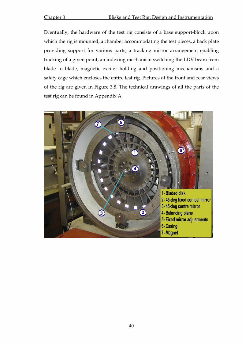
Chapter 3 Blisks and Test Rig: Design and Instrumentation
40
Eventually, the hardware of the test rig consists of a base support-block upon
which the rig is mounted, a chamber accommodating the test pieces, a back plate
providing support for various parts, a tracking mirror arrangement enabling
tracking of a given point, an indexing mechanism switching the LDV beam from
blade to blade, magnetic exciter holding and positioning mechanisms and a
safety cage which encloses the entire test rig. Pictures of the front and rear views
of the rig are given in Figure 3.8. The technical drawings of all the parts of the
test rig can be found in Appendix A.

Chapter 3 Blisks and Test Rig: Design and Instrumentation
41
Figure 3.8 Mistuning and damping test rig
3.3.2 Test chamber
The test chamber consists of a back plate and a cylindrical part, which are made
of steel, and a polycarbonate front cover. This polycarbonate front cover is
interchangeable with a transparent glass window to allow various measurement
techniques that are also explained in this chapter. Since the rig runs in vacuum,
all the joints and mountings are sealed. Other than sealing of bearing housing
where lip seals are more appropriate, O-rings have mostly been used for the
sealing. The casing is secured to a concrete block with slotted steel inserts, which
eases mounting of the rig to the base.
An air-free 0.37 kW Varian SH100 vacuum pump is used to evacuate the air in
the chamber. This way, additional complications such as aerodynamic damping,
blade coupling through fluid motion, blisk heating are prevented. Therefore, a
high standard vacuum is not needed. A relatively crude vacuum gauge with 0.02

Chapter 3 Blisks and Test Rig: Design and Instrumentation
42
bar pressure increments is used to observe the vacuum. The air leakage, if there
was any, was less than the gauge could successfully measure.
As the chamber is evacuated, the front cover, back plate and cylindrical parts are
all subjected to atmospheric pressure. Moreover, the cylindrical steel part is
required to be strong enough to withstand impact loads in the event of a
catastrophic failure such as blade loss under rotation. An FE model of the
chamber is prepared and analysed under the mentioned loading to verify the
design. The force resulting from a blade loss is modelled as a steady, static force.
The FE model and results are given in Figure 3.9. The maximum equivalent Von
Mises stress was calculated as 200 MPa for a yield strength of 420 MPa, resulting
in an adequate safety factor of 2.1.
Figure 3.9 FE model of the casing and analysis results
3.3.3 Drive system
The operating speed limit was decided to be 4000 rev/min in Section 3.2. As the
entire speed range (0-4000 rev/min) is to be swept in measurements, the drive
shaft should be designed such that its critical speeds occur outside this range.
An FE based critical speed calculation code RotFE [84] was used to calculate
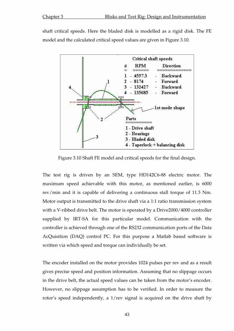
Chapter 3 Blisks and Test Rig: Design and Instrumentation
43
shaft critical speeds. Here the bladed disk is modelled as a rigid disk. The FE
model and the calculated critical speed values are given in Figure 3.10.
Figure 3.10 Shaft FE model and critical speeds for the final design.
The test rig is driven by an SEM, type HD142C6-88 electric motor. The
maximum speed achievable with this motor, as mentioned earlier, is 6000
rev/min and it is capable of delivering a continuous stall torque of 11.3 Nm.
Motor output is transmitted to the drive shaft via a 1:1 ratio transmission system
with a V-ribbed drive belt. The motor is operated by a Drive2000/4000 controller
supplied by IRT-SA for this particular model. Communication with the
controller is achieved through one of the RS232 communication ports of the Data
AcQuisition (DAQ) control PC. For this purpose a Matlab based software is
written via which speed and torque can individually be set.
The encoder installed on the motor provides 1024 pulses per rev and as a result
gives precise speed and position information. Assuming that no slippage occurs
in the drive belt, the actual speed values can be taken from the motor’s encoder.
However, no slippage assumption has to be verified. In order to measure the
rotor’s speed independently, a 1/rev signal is acquired on the drive shaft by

Chapter 3 Blisks and Test Rig: Design and Instrumentation
44
means of an optical sensor. It must be noted that this 1/rev signal is also
necessary for phase measurements as it provides a reliable trigger signal for the
vibration measurements. For this purpose a high-reflectivity small mirror is
glued to one of the flanges on the drive shaft and the optical sensor is secured to
a fixed base and at a prescribed distance to the small mirror. Each time the
mirror rotates past the optical sensor, a pulse is generated. Created pulses then
are fed into a simple circuit where the analogue signals are converted to digital
TTL pulses. By counting the number pulses in a given period of time, the
rotational speed is calculated. However, the accuracy of this kind of
measurement depends on the sampling frequency of the acquisition board, and
especially when precise speed measurements are required, very high sampling
frequencies are needed. As the vibration, force and 1/rev signals are acquired
via the same DAQ board and a few seconds worth of vibration signal is
necessary for proper signal processing, using high sampling frequencies is quite
costly since the same sampling frequency is dictated for all channels by the DAQ
board. As a result, some tests are carried out with very high (up to 200 kHz)
sampling rates to find out the amount of variation between rotor and motor side
speed values. The summary of performed tests is given in Table 3.3. It is clear
from this table that as the speed increases so does the deviation. This can be
attributed to the decrease in number of points acquired per rotation as the speed
increases since the same (maximum available) sampling frequency is used for all
measurements. Based on this evidence the difference is attributed to inadequate
sampling frequency rather than the slippage in the belt and therefore the
measurements taken on the motor side are regarded as the true speed values.
Nominal 120 300 600 1200 1800 2400
Motor encoder 120.01 299.93 600.1 1199.95 1800.05 2399.91
1/rev signal 120.04 300.21 600.5 1200.7 1801.1 2401.9
% difference 0.02 0.04 0.07 0.07 0.07 0.08
Table 3.3 Comparison of speed values on motor and rotor side (all speed values in rev/min)
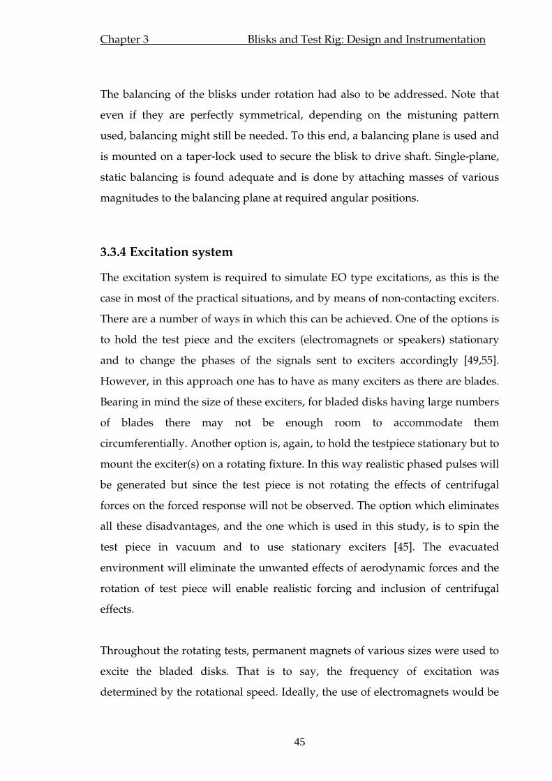
Chapter 3 Blisks and Test Rig: Design and Instrumentation
45
The balancing of the blisks under rotation had also to be addressed. Note that
even if they are perfectly symmetrical, depending on the mistuning pattern
used, balancing might still be needed. To this end, a balancing plane is used and
is mounted on a taper-lock used to secure the blisk to drive shaft. Single-plane,
static balancing is found adequate and is done by attaching masses of various
magnitudes to the balancing plane at required angular positions.
3.3.4 Excitation system
The excitation system is required to simulate EO type excitations, as this is the
case in most of the practical situations, and by means of non-contacting exciters.
There are a number of ways in which this can be achieved. One of the options is
to hold the test piece and the exciters (electromagnets or speakers) stationary
and to change the phases of the signals sent to exciters accordingly [49,55].
However, in this approach one has to have as many exciters as there are blades.
Bearing in mind the size of these exciters, for bladed disks having large numbers
of blades there may not be enough room to accommodate them
circumferentially. Another option is, again, to hold the testpiece stationary but to
mount the exciter(s) on a rotating fixture. In this way realistic phased pulses will
be generated but since the test piece is not rotating the effects of centrifugal
forces on the forced response will not be observed. The option which eliminates
all these disadvantages, and the one which is used in this study, is to spin the
test piece in vacuum and to use stationary exciters [45]. The evacuated
environment will eliminate the unwanted effects of aerodynamic forces and the
rotation of test piece will enable realistic forcing and inclusion of centrifugal
effects.
Throughout the rotating tests, permanent magnets of various sizes were used to
excite the bladed disks. That is to say, the frequency of excitation was
determined by the rotational speed. Ideally, the use of electromagnets would be

Chapter 3 Blisks and Test Rig: Design and Instrumentation
46
preferable as the frequency of excitation could be varied independently of
rotational speed. However, the force produced via these magnets was so small
that the required magnitudes could only be generated when they were placed at
very close proximity of the blisks. This was considered unsafe under rotating
conditions that the use of electromagnets was confined only to the static
measurements. Almost all of the tests (although for some friction-damped tests 2
magnets were used briefly) were carried out by using only one magnet. The
permanent magnet is secured to a holding and positioning mechanism such that
the magnetic force is exerted on the blade tips. The magnet and the holding
system are connected via a force transducer which measures the magnet’s
reaction in the presence of a passing blade, and the holding mechanism is
secured to the back plate. The magnet’s proximity to the bladed disks is adjusted
via a stepper motor which can be controlled from the DAQ PC through a code
written in Matlab. The gap can also be adjusted manually using a knob. A cross
section of the excitation system is given in Figure 3.11.
Figure 3.11 Excitation system
Mainly two different types of permanent magnets supplied by MagnetSales
company (http://www.magnetsales.co.uk/) are used. For mistuning tests on
Blisk-2 a Samarium deep-pot magnet (SMDP-00163, ∅20) with 25 kg maximum
pull force is used. Whereas for tests with friction dampers on Blisk-1 a magnet of

Chapter 3 Blisks and Test Rig: Design and Instrumentation
47
the same type but having a 40 kg maximum pull force (SMDP-00105, ∅25) is
used. This is necessary, as higher forces are required to make dampers work
effectively.
3.3.5 Vibration measurement system
As stated in the design requirements, the response measurement transducer
must be a non-contacting one so as not to perturb the tested structure’s
dynamics. That is to say, traditional techniques such as strain gauge—slip ring
or telemetry arrangements cannot be employed. As a non-contacting
measurement technique, “tip-timing” has been used with considerable success
for turbomachinery blade vibration measurements where an electromagnetic or
optical probe attached to the turbomachine casing is used to measure the blade
tip arrival times as they rotate past this probe. In the presence of vibration, each
blade passes the probe earlier or at a later time compared to non-vibrating case,
depending on the phase of their vibration at the time of arrival. Further
processing these arrival times, the vibration in the tangential direction is
obtained. This implies that the technique cannot be used with Blisk-2 as no
vibration in this direction for the family of modes of interest is produced.
Additionally, the use of this technique requires particular expertise, and high-
standard equipment and positioning tolerances to resolve the required
information.
As a result, it was decided to use an LDV transducer. Besides being a non-
contacting device, the LDV offers acquisition of spatially dense measurements in
fairly short times as well as providing easier instrumentation. Two vibration
measurement techniques; one using a tracking LDV and another using a
scanning LDV are used. Most of the rotating vibration measurements are
performed using the first, so called the self-tracking system. Several techniques
using scanning LDV are also used, mainly on stationary blisks, to measure radial
and circumferential deflection shapes and the direction of vibration.
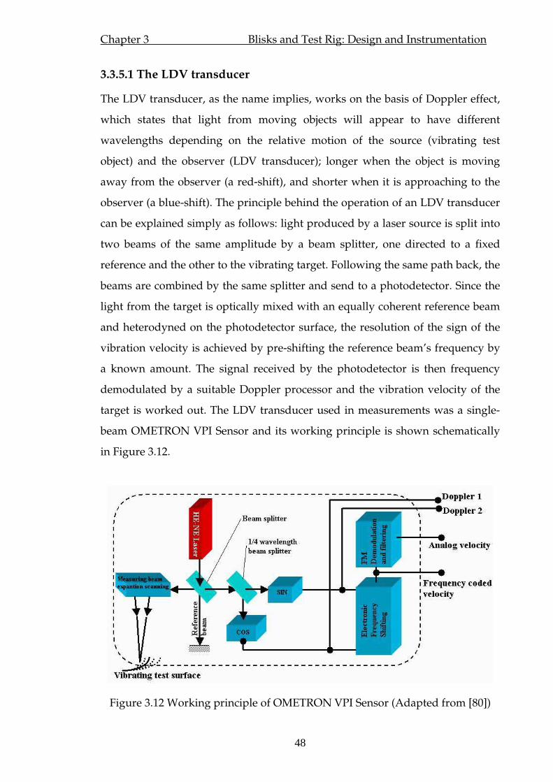
Chapter 3 Blisks and Test Rig: Design and Instrumentation
48
3.3.5.1 The LDV transducer
The LDV transducer, as the name implies, works on the basis of Doppler effect,
which states that light from moving objects will appear to have different
wavelengths depending on the relative motion of the source (vibrating test
object) and the observer (LDV transducer); longer when the object is moving
away from the observer (a red-shift), and shorter when it is approaching to the
observer (a blue-shift). The principle behind the operation of an LDV transducer
can be explained simply as follows: light produced by a laser source is split into
two beams of the same amplitude by a beam splitter, one directed to a fixed
reference and the other to the vibrating target. Following the same path back, the
beams are combined by the same splitter and send to a photodetector. Since the
light from the target is optically mixed with an equally coherent reference beam
and heterodyned on the photodetector surface, the resolution of the sign of the
vibration velocity is achieved by pre-shifting the reference beam’s frequency by
a known amount. The signal received by the photodetector is then frequency
demodulated by a suitable Doppler processor and the vibration velocity of the
target is worked out. The LDV transducer used in measurements was a single-
beam OMETRON VPI Sensor and its working principle is shown schematically
in Figure 3.12.
Figure 3.12 Working principle of OMETRON VPI Sensor (Adapted from [80])
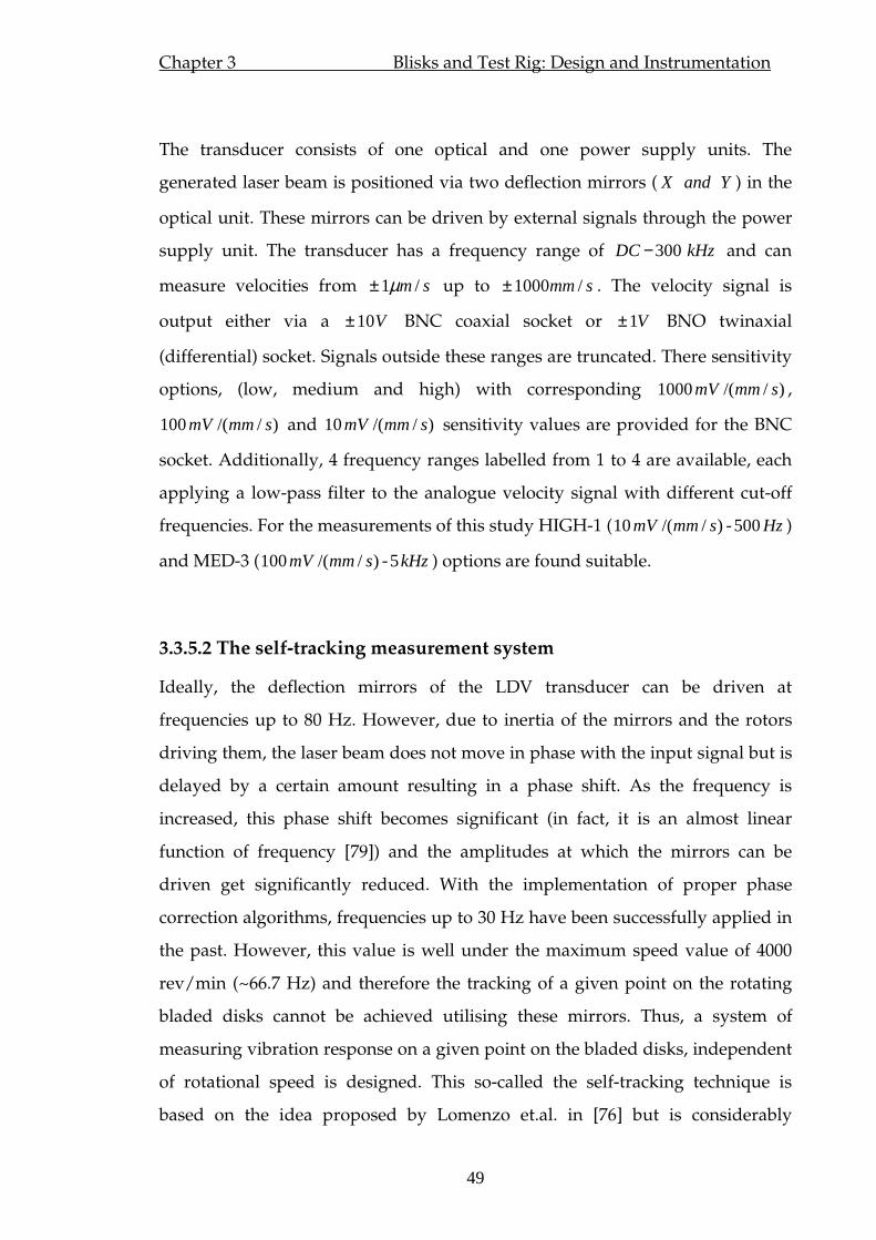
Chapter 3 Blisks and Test Rig: Design and Instrumentation
49
The transducer consists of one optical and one power supply units. The
generated laser beam is positioned via two deflection mirrors ( YandX ) in the
optical unit. These mirrors can be driven by external signals through the power
supply unit. The transducer has a frequency range of kHzDC 300− and can
measure velocities from sm/1µ± up to smm/1000± . The velocity signal is
output either via a V10± BNC coaxial socket or V1± BNO twinaxial
(differential) socket. Signals outside these ranges are truncated. There sensitivity
options, (low, medium and high) with corresponding )//(1000 smmmV ,
)//(100 smmmV and )//(10 smmmV sensitivity values are provided for the BNC
socket. Additionally, 4 frequency ranges labelled from 1 to 4 are available, each
applying a low-pass filter to the analogue velocity signal with different cut-off
frequencies. For the measurements of this study HIGH-1 ( )//(10 smmmV - Hz500 )
and MED-3 ( )//(100 smmmV - kHz5 ) options are found suitable.
3.3.5.2 The self-tracking measurement system
Ideally, the deflection mirrors of the LDV transducer can be driven at
frequencies up to 80 Hz. However, due to inertia of the mirrors and the rotors
driving them, the laser beam does not move in phase with the input signal but is
delayed by a certain amount resulting in a phase shift. As the frequency is
increased, this phase shift becomes significant (in fact, it is an almost linear
function of frequency [79]) and the amplitudes at which the mirrors can be
driven get significantly reduced. With the implementation of proper phase
correction algorithms, frequencies up to 30 Hz have been successfully applied in
the past. However, this value is well under the maximum speed value of 4000
rev/min (~66.7 Hz) and therefore the tracking of a given point on the rotating
bladed disks cannot be achieved utilising these mirrors. Thus, a system of
measuring vibration response on a given point on the bladed disks, independent
of rotational speed is designed. This so-called the self-tracking technique is
based on the idea proposed by Lomenzo et.al. in [76] but is considerably

Chapter 3 Blisks and Test Rig: Design and Instrumentation
50
modified. Here most notably the fold mirror of [76] is replaced by a fixed
annular conical mirror. This way laser beam can be sent to the blade tips at a
right angle. Additionally a means of switching measurements from blade to
blade is introduced. The devised tracking system is given in Figure 3.13.
Figure 3.13 The self-tracking system
In Figure 3.13, the laser beam passes through the small centre glass window in
the centre of the polycarbonate front cover and lands on the central 45-degree
small mirror rotating with the bladed disk. It then is directed to the fixed 45-
degree conical mirror before it finally arrives at a particular blade tip. The
central small mirror is mounted on a spring-loaded push rod which runs all the
way through the drive shaft to the rear end of the rig where it is fitted with a
slotted mechanical indexing device. The push rod is integrated with 3 pins at 120
degrees which sit on a 24-tooth bevel gear fixed to the drive shaft thus enabling
their engagement. When the pneumatic actuator is powered, it moves the push
rod forward consequently disengaging it from the drive shaft. Since the indexing
device moves with the push road, guided pins in the slots of indexing device
force the push rod to be rotated as well as moving forward, precisely by 15

Chapter 3 Blisks and Test Rig: Design and Instrumentation
51
degrees at each push. When the pneumatic actuator is released, the now
compressed spring moves the push road straight back without rotating it. Since
the angle between two neighbouring blades is 15 degrees, the laser beam is now
directed to the next blade. With the release of pneumatic actuator the pins on
push rod sit back on the bevel gear only shifted by 15 degrees. Details of
indexing mechanism can be seen in Figure 3.14. As this process can be
performed during the operation of the rig, all the blade responses can be
measured without interrupting the measurement session.
Figure 3.14 Indexing mechanism
The indexing mechanism described above requires the operator to push a button
each time a new blade is to be measured. However this process can easily be
automated by designing a simple circuit in combination with a timer/counter
card or a simple chip capable of processing commands sent via RS232. As a
result the laser beam can be automatically switched to the next blade once the
measurements on the current blade are completed. This can save considerable
time when the measurements are to be carried out for various speed values (see
Section 3.4.2).

Chapter 3 Blisks and Test Rig: Design and Instrumentation
52
3.3.5.3 Scanning system
Mainly two scanning techniques are used Conical Circular Scanning and Line
Scanning, which are both shown in Figure 3.15 (a) and (b) respectively. In case of
circular scan the external mirrors (fixed conical and small centre mirrors) and
mechanical indexing are not used and polycarbonate front cover is replaced by a
fully transparent, hardened glass window to enable optical access. The blisks
then can be scanned at a frequency Ω in a circle, by applying suitable
)( α+⋅Ω tSin , and )( β+⋅Ω tCos , waves to the LDV-integral beam-deflection
mirrors. Here the arbitrary phase angles α and β are introduced to account for
phase correction due to mirror delay. Since the bladed disks are discontinuous at
the blade tips, measurements in this system are taken at the near-continuous
platform edges and circumferential ODSs are extracted. In case of line scan the
blisks are scanned along the blade lengths to measure radial ODSs. This is used
in static measurements only and the blisks are oriented such that the blade
measured is vertical so that one mirror can be used for scanning. Both
techniques when applied to stationary blisks are excited by an electromagnet at
desired frequencies.
Figure 3.15 (a) Conical Circular Scan, (b) Line Scan
3.3.5.4 LDV alignment
Despite its major advantage of working regardless of rotational speed, the self-
tracking system is prone to misalignment problems, as indeed all other LDV

Chapter 3 Blisks and Test Rig: Design and Instrumentation
53
measurement techniques are. In an ideal arrangement, the laser beam is normal
to the plane of rotation of the test piece. The deviations from this plane will
result in errors in the position of the laser beam as well as in the measured
vibration velocity. Misalignment errors in this particular test setup are mainly
introduced in either because (i) the laser beam is not aligned with the axis of
rotation (Figure 3.16 (a) ), and/or (ii) fixed conical mirror’s position is not
properly adjusted with respect to the test piece (Figure 3.16 (b) ). In a misaligned
setup, the LDV signal will contain a proportion of the blade rotation velocity, at
rig rotation frequency, as demonstrated in Figure 3.16 (c).
Time
Ampl
itude
1 rev
(c)
Figure 3.16 Sources of misalignment (a, b) and its reflection on velocity signal (c).
As it is evident from Figure 3.16 (c), misalignment introduces slow frequency
oscillations (1 per rev in this case) on top of normal vibration frequency. Though
this can be eliminated by applying a high pass filter, it has been observed that in
some cases misalignment causes DAQ board to overload for signals it would not
if the alignment was perfect. This happens because peak-to-peak amplitude of
the signal is increased (see Figure 3.16 (c)). Additionally, misalignment may vary
the measurement spot with respect to the test piece introducing measurement
uncertainties. In order to alleviate these effects, the position of LDV head and
orientation of the fixed conical mirror should be checked and properly adjusted,
if necessary, before a measurement session is started. In order to achieve this, the
LDV head is placed on a milling machine traverse which enables precise

Chapter 3 Blisks and Test Rig: Design and Instrumentation
54
horizontal and vertical adjustments. In addition, an adjustable 4–leg platform is
placed between the LDV and the milling machine which provides a means to tilt
the LDV head. Horizontal rotation of the head is done by the operator. The
correction of the fixed conical mirror’s orientation is done via an adjustment
mechanism in which in-plane translation and out-of-plane rotation of the mirror
can be controlled. Details of both the LDV head and fixed mirror adjustment
configurations are shown in Figure 3.17.
Figure 3.17 (a) The LDV head and (b) the fixed mirror positioning details
in Figure 3.18
! "
#
$ % $
& $
' ( $
) $
# $
* $
*
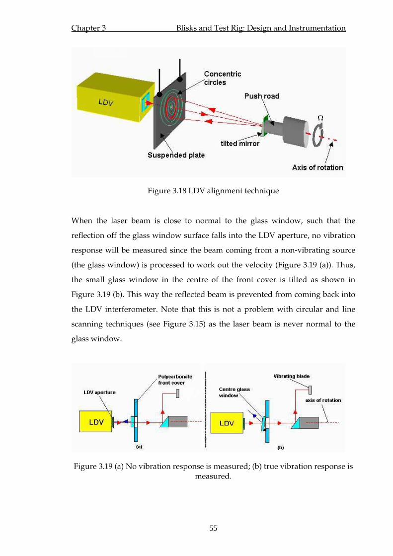
Chapter 3 Blisks and Test Rig: Design and Instrumentation
55
Figure 3.18 LDV alignment technique
When the laser beam is close to normal to the glass window, such that the
reflection off the glass window surface falls into the LDV aperture, no vibration
response will be measured since the beam coming from a non-vibrating source
(the glass window) is processed to work out the velocity (Figure 3.19 (a)). Thus,
the small glass window in the centre of the front cover is tilted as shown in
Figure 3.19 (b). This way the reflected beam is prevented from coming back into
the LDV interferometer. Note that this is not a problem with circular and line
scanning techniques (see Figure 3.15) as the laser beam is never normal to the
glass window.
Figure 3.19 (a) No vibration response is measured; (b) true vibration response is measured.

Chapter 3 Blisks and Test Rig: Design and Instrumentation
56
3.3.5.5 On the limitations of LDV transducers
While intrusive measurement techniques are not suitable for the current study,
the LDV transducers are not without their own complications. Since these are
optical devices, line of sight is a necessity which may not always be the case,
especially when some internal components are of interest. Moreover, though not
a problem for the self-tracking system, the application of scanning LDV to a
rotating structure is limited to relatively low speeds. This together with the strict
alignment requirements mean that the in-situ use of these transducers on
realistic structures such as turbine jet engines is still a remote possibility.
Furthermore, despite some attempts made at applying them to impact modal
testing [81], their application has been mostly confined to measuring one
frequency at a time.
One of the most important problems in LDV measurements is the sudden sharp
jumps, or dropouts, in velocity signal due to so called speckle noise and
demands a closer look as it limits the accuracy of the measurements, typically to
1% [79]. The speckle noise is a phenomenon related to speckle pattern which is
formed when surface roughness of the test object is comparable with the
wavelength of the laser light. In most of the real applications the test surface is
comparably rough and the light reflected back from the LDV has a granular
appearance referred to as speckle pattern. This pattern changes as the location of
the laser beam changes on the test surface and tends to get coarser as the laser
beam spot gets smaller. Therefore for a correctly focused laser beam the intensity
of light collected by the LDV fluctuates strongly as the laser beam moves on the
test surface. When the Doppler signal amplitude is lower than a threshold value,
the demodulation circuit in LDV cannot function properly and results in
“dropouts” in velocity signal [80]. This impairs the quality of the measurements
and limits the performance of the measurement system
For the self tracking measurements, once the laser beam is focused and a proper
velocity signal is received, assuming that this spot does not change in time, the

Chapter 3 Blisks and Test Rig: Design and Instrumentation
57
speckle noise will not be a problem. However this requires that the amplitude of
vibration is not large enough to cause the measurement spot to change and that
the LDV beam to be perfectly aligned with the axis of the rotation of the test
structure. In practice, though it can be eliminated to a great extend (see previous
section), misalignment cannot be removed completely and causes the laser spot
to move across the test piece, making the velocity signal more susceptible to
speckle noise. The same effect can be observed when the large vibration
amplitudes are present. A typical example demonstrating the coupled effect of
both the misalignment and large vibration amplitudes is given in Figure 3.20. In
Figure 3.20 (a) tracking measurement on a particular blade under rotation is
given. Here a frequency modulation due to misalignment and amplitude
modulation due to dropouts caused by speckle noise are observed. Note that the
dropouts are periodic (see point A in Figure 3.20 (a)), occurring at the same
locations on the structure. When the amplitude of input force is reduced, Figure
3.20 (b), thus reducing the vibration amplitude, the dropouts and consequently
the amplitude modulation is eliminated. However, the misalignment remains
unaffected. The reflection of these dropouts in the frequency spectrum is in the
form additional pseudo-frequency components, Figure 3.20 (c) which are not
present otherwise, Figure 3.20 (d). When EO response is to be extracted, the
presence of speckle noise does not introduce errors in the frequency but may
slightly modify the amplitudes. However, when for example, a z-mod plot is to
be constructed using frequency spectra alike, one has to pay attention, as these
pseudo-components will appear as resonances.

Chapter 3 Blisks and Test Rig: Design and Instrumentation
58
-15
-10
-5
0
5
10
0
2
4
6
8
10
Am
p. (V
)
-10
-5
0
5
10Time
0
2
4
6
8
Am
p. (V
)
Frequency
A A A
Dropouts
Pseudo frequency components
(a)
(b)
(c)
(d)
Figure 3.20 Velocity signals with (a), and without (b) dropouts, and the corresponding frequency spectra, (c) and (d).
The adverse effects of speckle noise, however, may be minimised by using a
proper working distance, applying reflective coating on the measurement
surface, properly focusing the laser beam and using a suitable sensitivity range
as all these precautions will increase the intensity of the light collected by the
LDV and make the signal strong enough to exceed the mentioned threshold. By
paying attention to above-mentioned precautions, in general, it has been
possible to acquire satisfactory velocity signals, both for tracking and scanning
measurements in this study, though there have been cases such as the one
shown in Figure 3.20. However, this meant that H-1 (i.e., minimum frequency
range) sensitivity level had to be used. Fortunately, the frequencies of interest
were within the range covered by this sensitivity option.
3.3.6 Safety provisions
It is demonstrated through FE analysis (Section 3.3.2) that the test chamber is
strong enough to withstand forces which may result due to failures such as
blade-loss. However in the event of bearing failure or sudden vacuum loss, the
blisks may come loose and the front covers used in the tests may be detached or
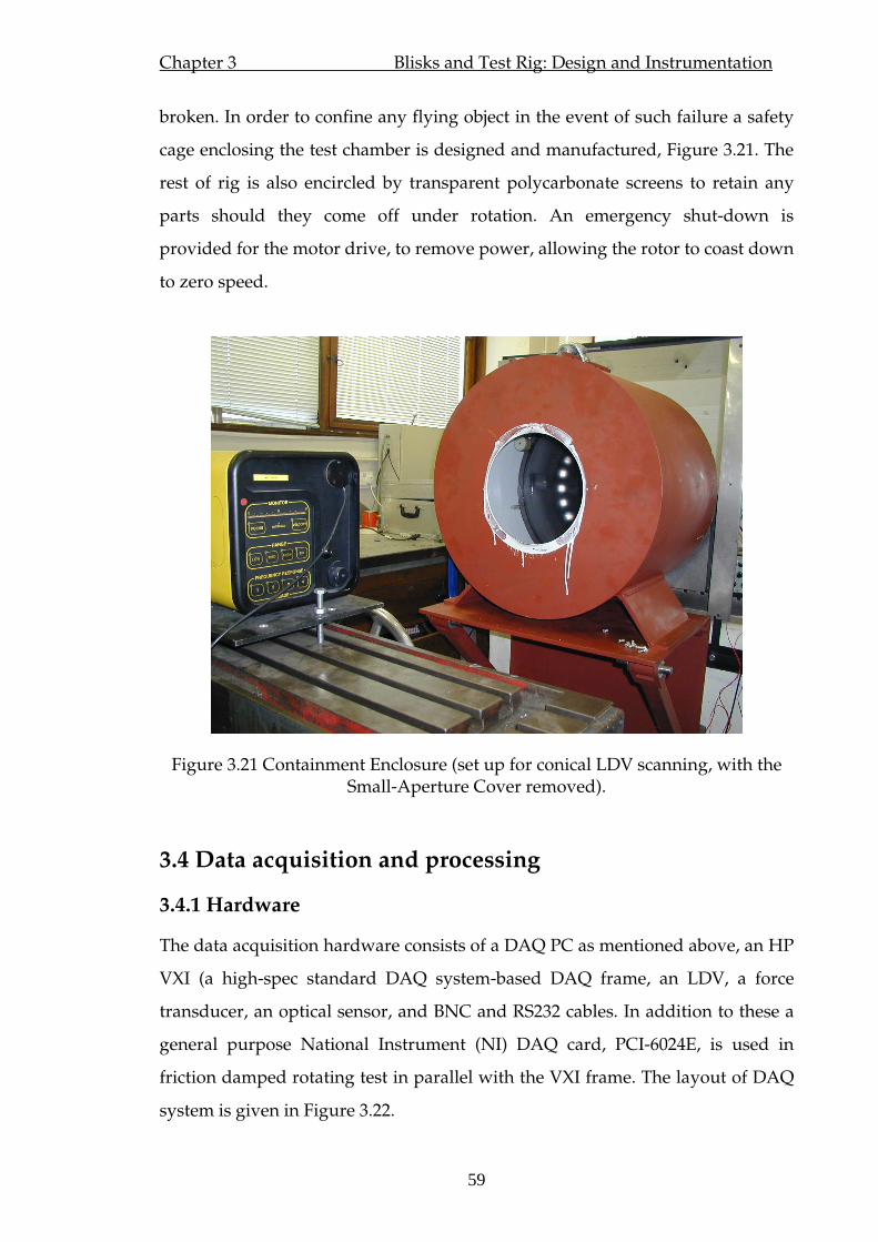
Chapter 3 Blisks and Test Rig: Design and Instrumentation
59
broken. In order to confine any flying object in the event of such failure a safety
cage enclosing the test chamber is designed and manufactured, Figure 3.21. The
rest of rig is also encircled by transparent polycarbonate screens to retain any
parts should they come off under rotation. An emergency shut-down is
provided for the motor drive, to remove power, allowing the rotor to coast down
to zero speed.
Figure 3.21 Containment Enclosure (set up for conical LDV scanning, with the Small-Aperture Cover removed).
3.4 Data acquisition and processing
3.4.1 Hardware
The data acquisition hardware consists of a DAQ PC as mentioned above, an HP
VXI (a high-spec standard DAQ system-based DAQ frame, an LDV, a force
transducer, an optical sensor, and BNC and RS232 cables. In addition to these a
general purpose National Instrument (NI) DAQ card, PCI-6024E, is used in
friction damped rotating test in parallel with the VXI frame. The layout of DAQ
system is given in Figure 3.22.
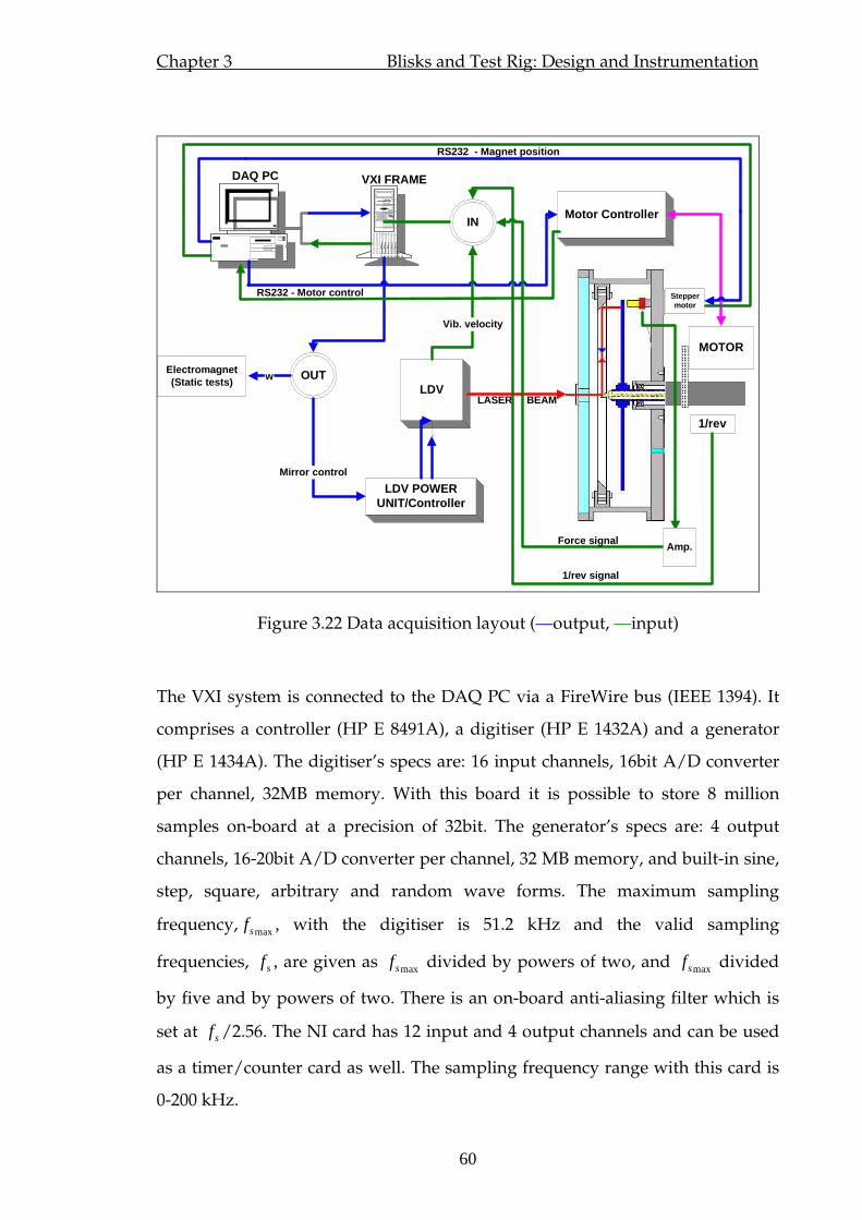
Chapter 3 Blisks and Test Rig: Design and Instrumentation
60
OUT
INMotor Controller
LDVLASER BEAM
LDV POWERUNIT/Controller
Vib. velocity
Steppermotor
MOTOR
Mirror control
w
1/rev
Amp.Force signal
1/rev signal
Electromagnet(Static tests)
RS232 - Magnet position
RS232 - Motor control
DAQ PC VXI FRAME
Figure 3.22 Data acquisition layout (—output, —input)
The VXI system is connected to the DAQ PC via a FireWire bus (IEEE 1394). It
comprises a controller (HP E 8491A), a digitiser (HP E 1432A) and a generator
(HP E 1434A). The digitiser’s specs are: 16 input channels, 16bit A/D converter
per channel, 32MB memory. With this board it is possible to store 8 million
samples on-board at a precision of 32bit. The generator’s specs are: 4 output
channels, 16-20bit A/D converter per channel, 32 MB memory, and built-in sine,
step, square, arbitrary and random wave forms. The maximum sampling
frequency, maxsf , with the digitiser is 51.2 kHz and the valid sampling
frequencies, sf , are given as maxsf divided by powers of two, and maxsf divided
by five and by powers of two. There is an on-board anti-aliasing filter which is
set at sf /2.56. The NI card has 12 input and 4 output channels and can be used
as a timer/counter card as well. The sampling frequency range with this card is
0-200 kHz.

Chapter 3 Blisks and Test Rig: Design and Instrumentation
61
In the long-run stepped-speed rotating measurements (i.e., measurement
sessions in which a given speed range is measured at given steps), sampling
frequencies of 800 Hz and 1280 Hz are mostly used depending on the max.
frequency of interest. The use of relatively small sampling rates has the
advantage of storing long data samples to carry out proper signal processing at
low costs. However when the phase information is to be extracted satisfactorily,
which is especially of interest in friction damper tests, these sampling
frequencies do not provide the necessary resolution. Since the same sampling
rates has to be used for all the channels of the VXI system, it has been decided to
use a second DAQ card, NI-PCI-6024E, to measure short samples at a relatively
high sampling rate to obtain accurate phase information. This way, using both of
the DAQ boards, the necessary information is collected while the data lengths
are kept manageable.
3.4.2 Data acquisition
High-level instrument control and data acquisition is done via a visual code
written in MATLAB The low-level drivers controlling the DAQ board are
provided by the manufacturer. The code consists of a main panel via which
appropriate input and output DAQ boards, channels and their attributes can be
specified; a motor control tool which sets and controls the motor speed, range
and steps; a magnet position tool which controls the stepper motor to adjust the
magnet-blade gap; an indexer tool which switches the laser beam from blade to
blade, and various processing tools to design band-pass filters, display/compare
ODSs etc. All the mentioned tools can be combined to complete a measurement
session automatically without user intervention. More details on the code and
snapshots of the user interface can be found in Appendix B.
Since a single static excitation source is used, frequency response curves for
various EO excitations are measured by changing the rotational speed. For an

Chapter 3 Blisks and Test Rig: Design and Instrumentation
62
nEO response, a rotational speed range around the nEOnND − lines crossing
is selected. Note that this location is fairly accurately estimated via FE models in
the test planning phase of the measurements. Then the discrete speed values at
which the response is acquired are decided. Generally, speed values are
clustered around resonances and coarser step sizes are used away from
resonances. The minimum speed change which can be achieved (i.e., the
minimum change in speed which makes sure that the new speed is higher or
lower than the previous value depending on the direction of sweep) is 1 to 2
rev/min (0.017-0.033 Hz) depending on the speed range used (see Table 3.3).
Then the motor speed is varied through this range and the vibration reponse
together with the force and 1/rev signal are streamed from the DAQ board for
each value in the range. The bladed disks used here are extremely lightly
damped when not fitted with external damping elements. In order to make sure
that the steady-state vibration levels are reached, it is necessary to wait up to one
minute each time the speed is changed to a new value. Assuming that k seconds
worth of data are to be acquired, and p seconds pause is necessary between
each speed change, the time it takes to complete a measurement session of N
speed points for all blades can be estimated as ( ) 24⋅∆++⋅ pkN seconds,
where ∆ is a computer-dependent value (time needed to stream and store the
data, and generally around 1 second). For a measurement session of 100 speed
points where 5 seconds worth of data is collected, and a minute’s pause is
introduced between each successive speed change, assuming 1=∆ second, the
required time to measure 24 blades is 44 hours! In a situation where the indexing
is automated and assuming that indexing the laser beam from blade to blade
takes 10 seconds, this time can be reduced to 12 hours. With implementation of a
proper timer/counter card, indexing time can be reduced to less than 5 seconds,
thus bringing the measurement time for this particular example under 10 hours.
Chapter 3 Blisks and Test Rig: Design and Instrumentation
63
3.4.3 Data processing
The methods of processing the force transducer and tachometer signals have
been given in previous sections. Here the processing of measured velocity signal
will be given. A flowchart explaining the various stages of frequency response
calculations is given in Figure 3.23. Note that since the excitation frequency is
varied by means of changing the rotor speed, this loop is repeated for all speed
values and engine orders, albeit in a computationally efficient way. Three ways
of calculating the EO frequency response are considered. In all cases, vibration
data are first low-pass filtered (anti-aliasing filter) and then flat-top windowed.
In the first option, the signal is band-pass filtered with a pass-band covering a
small range around the desired vibration frequency (i.e.,
δδ +Ω⋅<Ω⋅<−Ω⋅ EOEOEO , where Ω is rot. speed and δ is a small
value such that only a few frequency bins are covered). Then an FFT is applied
and the maximum amplitude of the output spectrum is recorded as the
amplitude of vibration at that particular speed value. In the second option, the
FFT is applied and the amplitude of the desired frequency is retrieved by finding
the maximum amplitude in the spectrum, in a frequency range similar to the one
given above. In the third option, assuming that the rotational speed is known
reasonably accurately, only the frequency bins at the frequency of vibration
( Ω*EO ) are calculated to obtain the frequency response.

Chapter 3 Blisks and Test Rig: Design and Instrumentation
64
FFT
FFT
PICK FREQ.BIN
w1<w<w2
PEAK theMAX Amp.
LOWPASSFILTER
FLATTOPWINDOW
MOVINGBANDPASSFILTER
SINGLE BINEXTRACTION
OUTPUT
INPUT
Cos(w),Sin(w)
32
1
Figure 3.23 Process of EO response calculation
In theory, all these options provide the same information. However, the first one
takes a considerable time to run since filtering is a computationally expensive
process. The last option is particularly useful, and especially so in phase
extraction, when only short data samples are available.
3.5 ODS measurements using CSLDV
As mentioned before, throughout the measurements several LDV scanning
techniques are made use of: line scan and circular scan for ODS measurements in
radial and circumferential directions respectively, and conical scan for direction
of vibration measurements. For the details of these techniques, references [77]
and [79] can be consulted. However, the circular scanning technique is
particularly of interest in the current study and is extensively used in stationary

Chapter 3 Blisks and Test Rig: Design and Instrumentation
65
blisk measurements as well as in some rotating ones. Thus, a brief explanation of
the theory and application is thought appropriate. An electromagnet is used to
excite the blisks to recover these ODSs under stationary conditions and a note on
the application of this kind of forcing is warranted.
3.5.1 Electromagnetic excitation
In fact, a.c magnet excitation is always attractive such that when driven by a
sinusoidal signal at nω , the excitation experienced by the structure is modified
and is at nω2 . However in the present case, it has been possible to excite the
blisks at a natural frequency, nω , by driving the magnet at the same frequency,
nω . In practice, when the blisks vibrate at frequency nω , the magnet-blade gap
is modulated at this frequency. Given the fact that the magnetic force is related
to the gap by an inverse square rule, a force input at frequency nω is generated
via this modulation. And it is this component that maintains the vibration.
Naturally, the degree of this effect depends on the modulation at the drive point,
which is maximised at natural frequencies. To understand this better consider
the sketch given in Figure 3.24. Assuming that the blade shown vibrates at
frequency, ω , the clearance between the magnet and the blade can be given by
)()( taSintx ωδ −= . (4.3)
Figure 3.24 Electromagnetic excitation on a stationary blade
)( txSinω
δ
x
a
Blade
Electromagnet
Chapter 3 Blisks and Test Rig: Design and Instrumentation
66
Suppose that the magnet is driven at the same frequency, ω , in the form
)()( tbSintf ω= , (4.4)
and recalling that the magnet force is always positive, the force experienced by
the blade may be related to the gap and the input force as follows
2
1( ) ( )
( ( ))F t bSin t
aSin tω
δ ω→
− (4.5)
Assuming above relation to be an exact representation of force, a typical force
signal calculated for a relatively small vibration amplitude, a (i.e. stiff blade or
large gap) is given in
Figure 3.25 (a). The corresponding frequency spectrum is also given in
Figure 3.25 (b) in which a dominant frequency component at 2ω is evident and
no force is produced at frequency ω . However, when the vibration amplitude,
a , is comparable to magnet-blade gap, δ , (i.e. flexible disk or small gap), the
forcing function takes the form given in
Figure 3.25 (c). In this case, the main frequency component is obtained at input
frequency ω (
Figure 3.25 (d)), as well as some other comparable components at its integer
multiples. The blisks used in this study are fairly flexible. Additionally the
magnet needed to be positioned reasonably close to the blade so that enough
force could be produced. Thus, the magnet blade gap was significantly
modulated, and especially at resonances, that blisks were excited by driving the
electromagnet at natural frequencies.
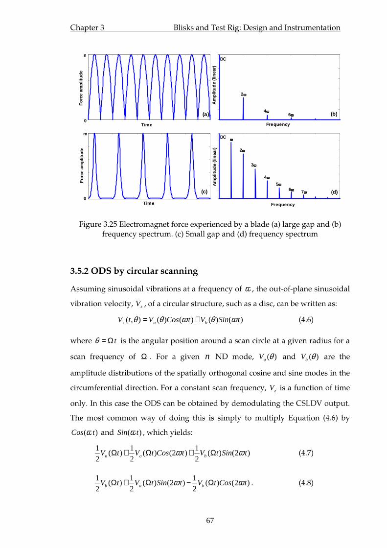
Chapter 3 Blisks and Test Rig: Design and Instrumentation
67
Frequency
For
ce a
mpl
itude
2ωωωω
4ωωωω 6ωωωω
ωωωω
2ωωωω
3ωωωω
4ωωωω
5ωωωω 6ωωωω 7ωωωω
0
0 Time
(a) (b)
(c) (d)
n
m
Time Frequency
Am
plitu
de (
linea
r)A
mpl
itude
(lin
ear)
For
ce a
mpl
itude
DC
DC
Figure 3.25 Electromagnet force experienced by a blade (a) large gap and (b) frequency spectrum. (c) Small gap and (d) frequency spectrum
3.5.2 ODS by circular scanning
Assuming sinusoidal vibrations at a frequency of ω , the out-of-plane sinusoidal
vibration velocity, zV , of a circular structure, such as a disc, can be written as:
)()()()(),( tSinVtCosVtV baz ωθωθθ += (4.6)
where tΩ=θ is the angular position around a scan circle at a given radius for a
scan frequency of Ω . For a given n ND mode, )(θaV and )(θbV are the
amplitude distributions of the spatially orthogonal cosine and sine modes in the
circumferential direction. For a constant scan frequency, zV is a function of time
only. In this case the ODS can be obtained by demodulating the CSLDV output.
The most common way of doing this is simply to multiply Equation (4.6) by
)( tCosω and )( tSin ω , which yields:
)2()(2
1)2()(
2
1)(
2
1tSintVtCostVtV baa ωω Ω+Ω+Ω (4.7)
)2()(2
1)2()(
2
1)(
2
1tCostVtSintVtV bab ωω Ω−Ω+Ω . (4.8)

Chapter 3 Blisks and Test Rig: Design and Instrumentation
68
If a sufficiently slow scan frequency is used, the frequency components at
around ω2 in Equations (4.7) and (4.8) can be removed by applying a low-pass
filter. Following that these equations yield real and imaginary parts of the ODS.
The LDV output from a sample circular scan session on Blisk-1 is given in Figure
3.26 (a). The blisk is scanned at platform level using a scan frequency of 0.5 Hz
while being excited by an a.c. magnet at a natural frequency. The individual
blade responses are clearly identifiable from the given circular scan output but
better demonstrated in Figure 3.26 (b). Note that dropouts occur in-between
blades since the platforms are discontinuous, and within a blade due to speckle
noise. The ODS obtained by demodulation is also given in Figure 3.27, in 3D and
2D form. The 2D option will be used from now on, as it is easier to visualise. The
number of nodal points and therefore the number nodal diameters is clearly
demonstrated, indicating a mostly real, smooth 4-ND mode. However, a non-
trivial imaginary part, in quadrature with the real, is also present. With this
technique, the identification of number of NDs in a given mode barely takes a
few seconds as demodulation can be carried out straight after the acquisition.
Figure 3.26 Slow circular scan LDV output

Chapter 3 Blisks and Test Rig: Design and Instrumentation
69
Figure 3.27 Real and imaginary parts of circumferential ODS
Assuming the blisk vibration to be at an n ND mode and substituting )(θCosVRn
for )(θaV , and )(θSinVIn for )(θbV , the expansion of Equation (4.6) gives:
( ) ( ) ( ) ( )2
( )2
Rn Inz Ro Io
Rn In
V VV t V Cos t V Sin t Cos n t
V VCos n t
ω ω ω
ω
+= + + − Ω
−+ + Ω (4.9)
The vibration velocity described by the above equation has frequency
components at )( Ω± nω . The spectrum, therefore, will have sidebands spaced at
Ω± n about the vibration frequency, ω . Some important properties can be
observed from Equation (4.9):
• When the mode being measured is purely real, the IV terms are all zero
and sidebands are of equal amplitude, indicating a pure standing wave in
the blisk
• When RV and IV are equal there exists only one sideband at )( Ω− nω ,
indicating a pure travelling wave, and finally
• When RV and IV are different than each other, the deflection shape will be
a combination of standing and travelling waves, the degree of which
being decided by the relative amplitudes of the sidebands (the difference
will indicate the travelling wave portion).

Chapter 3 Blisks and Test Rig: Design and Instrumentation
70
The LDV output of the same mode given in Figure 3.28, scanned at Ω =5Hz ,
together with the corresponding frequency spectrum is given in Figure 4.25.
Since the sidebands are separated by Ωn2 , the identification of the number of
NDs, n , is straightforward: 40/(2*5)=4. Note that the frequency spectrum
contains additional, relatively small, amplitude sidebands, again centred about
the vibration frequency, indicating the existence of other ND mode components
in the deflection shape. Here the mode observed is mainly a standing wave with
slight difference in sideband amplitudes, thus hinting at the presence of some
travelling wave portion as well (inline with the findings in Figure 3.27). Even
then, the amplitude at the frequency of vibration, ω , is indistinguishable from
the noise floor.
0 0.2 0.4 0.6 0.8 1 1.2 1.4 1.6 1.8 2-10
-5
0
5
10
Time (s)
Am
plitu
de (V
)
150 200 250 300 350 4000
1
2
3
Frequency (Hz)
Am
plitu
de (V
)
231 Hz 271 Hz
271 - 2312*5
=4n=
ωωωω=251Hz
ωωωω-nΩΩΩΩ ωωωω+nΩΩΩΩ
(a)
(b)
Figure 3.28 (a) Circular scan LDV output, and (b) the frequency spectrum
3.6. Validation of measurement setup
The vibration and force measurement setups need to be validated against
independent alternative techniques in the way the speed measurements were
validated in Section 4.2.3. Here the calibration of the transducers used in the
alternative measurements is not given as standard procedures are followed in
ensuring this.

Chapter 3 Blisks and Test Rig: Design and Instrumentation
71
3.6.1 Vibration measurement setup validation
The use of the LDV transducer with circular and line scanning methods was
validated against traditional response measurement techniques in [79], and good
qualitative and quantitative agreements were obtained. However, the same
needs to be repeated for the self-tracking system as well. To this end, a B&K
accelerometer is used to measure the vibration on a blade. Note that the
instrumentation in this case dictates the bladed disk to be tested at rest. Impact
response at a particular blade tip is measured by the LDV transducer and the
accelerometer simultaneously so that the response to the same force input can be
measured. The comparison of the acquired impact responses covering a
frequency range mostly used in tests are given in Figure 3.29. Note that the LDV
measures velocity therefore the corresponding signal is differentiated once to get
the acceleration so that it can be compared to the accelerometer’s output. The
excellent agreement between both measurements confirms the validation of
vibration measurement setup.
80 100 120 140 160 180 200 220 240 260
-15
-10
-5
0
5
10
15
20
25
30
35
Frequency (Hz)
Am
plitu
de (d
B) -
re 1
ms
-2/N
Ometron VPI SensorEndevco 2222C acc.
Figure 3.29 Comparison of LDV and accelerometer outputs

Chapter 3 Blisks and Test Rig: Design and Instrumentation
72
3.6.2 Force measurement setup validation
The validation of excitation system requires an elaborate setup compared to
vibration setup. Here the validation is carried out in two steps. In the first step,
the static deflection of a blade is measured for various force values using a non-
contacting proximity probe (Bently Nevada). The forces are applied via a pulley
system by utilising the tapped hole in the tip of the blade. Metal pieces of known
quantity are hung by a string, which eventually is tied to a bolt screwed into the
tapped hole in the tip of the blade. This way the force is applied normal to the
blade simulating the magnetic force. The proximity probe is brought near to the
unloaded blade and the measured value is taken as the reference zero. Than
relative readings are recorded as the payload is increased. In the second step,
again, the blade position relative to the probe is first measured in the absence of
magnetic force by retracting the magnet. In this case, no force is registered by the
force transducer. It is made sure that the same reference value is achieved by
adjusting the blade-probe distance. Then the magnet is advanced to close
proximity of the blade in precise increments by controlling the stepper motor via
the DAQ PC. The relative readings are again recorded at various blade-magnet
gaps. Later, the force transducer signals at exactly the same stations where the
probe measurements were taken are acquired. The variation of the proximity
probe’s output with increasing payload is given in Figure 3.30 (a). A perfectly
linear relation, as expected, is obtained. Later, using this relation, the relative
readings of magnet-imposed deflections are converted into corresponding force
values and are compared to the force transducer’s readings. This comparison is
given in Figure 3.30 (b). The range of applied magnetic forces covers the typical
values used in the experiments. Overall, a good match is obtained between the
estimated and force transducer measured magnet forces with an error less than
3.6%.

Chapter 3 Blisks and Test Rig: Design and Instrumentation
73
0 0.2 0.4 0.6 0.8 1 1.2 1.40
200
400
600
800
1000
1200
Relative probe output (V)
Dea
d w
eigh
t (gr
am)
Y = 1000*X + 14
Measured dataLinear fit
0 0.5 1 1.5 22
4
6
8
10
12
14
16
18
20
Relative probe output (V)
For
ce (N
)
3.6
0.57
0.57
0.69EstimatedForce transducer
% Difference
(a) (b)
Figure 3.30 Force measurement setup validation
3.7 Summary In this chapter the design and manufacture of blisks to be used in mistuned and
friction damped vibration response measurements is given. Through FE
analyses, the blisks are designed to reflect the design requirements. Based on the
computed Campbell diagrams, a maximum speed limit is chosen to be 4000
rev/min, covering most of the resonances (i.e., 4D and above) corresponding to
the 1F family of modes for both blisks.
The design and instrumentation details of a rig to be used in the tests have also
been presented. The rig runs in a vacuum so that unwanted aerodynamic effects
are excluded. Through FE analyses, the test enclosure and drive shaft were
designed to withstand possible operational forces. Speed and phase
measurement methods are introduced. A variable-gap permanent magnet
excitation mechanism is implemented. The rig design allows the use of up to six
exciters. A special mirror arrangement and indexing mechanism were designed
to address the need to track a point on a rotating structure. This so-called self-
tracking system works independently of rotation speed.
The employed LDV transducer is introduced. Two measurement techniques are
described: one using tracking LDV to measure blade tip vibration responses, and

Chapter 3 Blisks and Test Rig: Design and Instrumentation
74
another using scanning LDV to measure ODSs in radial and circumferential
directions. The steps which need to be taken to align the LDV with the axis of
rotation are explained. The limitations, as well as the advantages, of LDV
measurements are stated. The effect of speckle noise on measurement quality
and its minimisation through improved surface reflectivity and alignment is
shown.
The DAQ hardware components and their connectivity are presented. The
software controlling the instrumentation and DAQ is also mentioned. Different
ways of data processing in obtaining EO frequency response curves are given.
The use of CSLDV in circumferential ODS recovery is presented through some
real measurements.
Finally, the used vibration and force measurement setups are validated through
independent measurements.
Chapter 4 Blisk Tuning, Model Updating and Test Design
75
CHAPTER 4
BLISK TUNING, MODEL
UPDATING and TEST DESIGN
4.1 Overview
So far we have concentrated on the design and development of the blisk
testpieces and the test rig, and have reported on the measurement tools and
techniques to be used in preparation of the real tests. However, before we go
about testing, there are a number of crucial steps which need to be taken in order
to make the test campaign time-efficient and to make sure that only useful data
are acquired. It is also necessary to ensure that the blisk models to be used in
predictions are good representations of the real ones. In this chapter, first, the
tuned states of blisks designed in Chapter 3 are identified and the blisks are
tuned when the tuning is deemed to be necessary. The sensitivity of a blisk’s
dynamic properties to various ways of tuning is investigated through a lumped
parameter model. Methods to be used in model updating are then introduced,
and based on the preliminary measurements on stationary blisks, the blisk
models are updated. Using these updated models, a comprehensive test plan is
designed and the selected configurations are justified through appropriate FE
analyses.
4.2 Tuning of blisks
The manufacture of blisks and their designed characteristics were given in the
previous chapter. However, before testing it is necessary to measure the actual
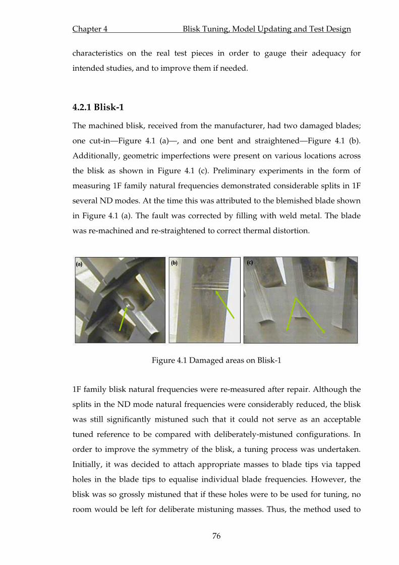
Chapter 4 Blisk Tuning, Model Updating and Test Design
76
characteristics on the real test pieces in order to gauge their adequacy for
intended studies, and to improve them if needed.
4.2.1 Blisk-1
The machined blisk, received from the manufacturer, had two damaged blades;
one cut-in—Figure 4.1 (a)—, and one bent and straightened—Figure 4.1 (b).
Additionally, geometric imperfections were present on various locations across
the blisk as shown in Figure 4.1 (c). Preliminary experiments in the form of
measuring 1F family natural frequencies demonstrated considerable splits in 1F
several ND modes. At the time this was attributed to the blemished blade shown
in Figure 4.1 (a). The fault was corrected by filling with weld metal. The blade
was re-machined and re-straightened to correct thermal distortion.
Figure 4.1 Damaged areas on Blisk-1
1F family blisk natural frequencies were re-measured after repair. Although the
splits in the ND mode natural frequencies were considerably reduced, the blisk
was still significantly mistuned such that it could not serve as an acceptable
tuned reference to be compared with deliberately-mistuned configurations. In
order to improve the symmetry of the blisk, a tuning process was undertaken.
Initially, it was decided to attach appropriate masses to blade tips via tapped
holes in the blade tips to equalise individual blade frequencies. However, the
blisk was so grossly mistuned that if these holes were to be used for tuning, no
room would be left for deliberate mistuning masses. Thus, the method used to

Chapter 4 Blisk Tuning, Model Updating and Test Design
77
adjust the state of tune of the blisk was to remove metal from the mass at the end
of each blade in turn, so that all the first family of natural frequencies were as
near identical as possible. In this way, all blade natural frequencies were to be
brought up the level of the highest-frequency blade. This process required
individual blades to be isolated so that their natural frequencies could be
measured, uninfluenced by the other blades on the blisk. To this end, the disc
was clamped between two massive blocks, up to the blade roots, and all blades,
apart from the one being tested, were interconnected – initially by modelling
clay (‘Plasticene’) and later with annular metal clamps, with a gap for the test
blade. Figure 4.2 shows the later test arrangement. The ‘Plasticene’ technique
was easier to use, but was found to be insufficiently consistent, and was
abandoned after the first check on the damaged blisk.
Figure 4.2 Test Arrangement used for measuring individual blade frequencies
Only the first natural frequencies for the isolated blades were tuned. The
variation of blade-alone frequencies for the blisk before repairs, after repairs and
after tuning are given in Figure 4.3 and statistics of these variations are given in
Table 4.1.
B&K acc.

Chapter 4 Blisk Tuning, Model Updating and Test Design
78
Figure 4.3 Variation of blade-alone natural frequencies
Min (Hz) Max (Hz) Mean (Hz) Std dev Max % dev. from mean
Original blisk 264.0 275.6 272.03 2.39 2.95
After Repairs 269.3 276.1 272.40 1.87 1.36
Tuned Blisk 282.0 283.0 282.38 0.32 0.22
Table 4.1 Statistics of blade-alone natural frequencies
Since the disk portion could not be fully clamped, due to disk-blade blend
geometry (see Figure 4.1), it was not possible to decouple the blades completely.
Although low-amplitude, non-trivial vibration signals were measured on the
clamped blades. In fact, since the blades were tuned in turn, as metal was
removed from the blade being tuned, the frequencies of other blades were
shifted, due to the non-negligible inter-blade coupling, to values which were
different to those they had at the time of the first measurement. As a result, it
was necessary to go round the blisk a few times to make sure that all the blade
frequencies were sufficiently close. Gross inherent mistuning in the blisk (mainly
due to poor manufacture) together with this iterative procedure, resulted,
unfortunately, in large masses being removed from blade tips (see the inset of
Figure 4.2). The “Original” and “After repairs” blade-alone measurements were
made by sticking a small accelerometer (0.5 gm Endevco 2222C) to blade tips
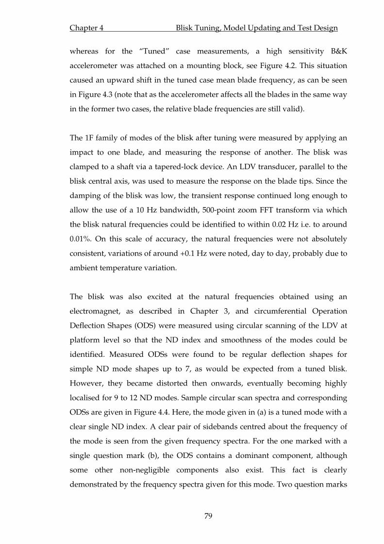
Chapter 4 Blisk Tuning, Model Updating and Test Design
79
whereas for the “Tuned” case measurements, a high sensitivity B&K
accelerometer was attached on a mounting block, see Figure 4.2. This situation
caused an upward shift in the tuned case mean blade frequency, as can be seen
in Figure 4.3 (note that as the accelerometer affects all the blades in the same way
in the former two cases, the relative blade frequencies are still valid).
The 1F family of modes of the blisk after tuning were measured by applying an
impact to one blade, and measuring the response of another. The blisk was
clamped to a shaft via a tapered-lock device. An LDV transducer, parallel to the
blisk central axis, was used to measure the response on the blade tips. Since the
damping of the blisk was low, the transient response continued long enough to
allow the use of a 10 Hz bandwidth, 500-point zoom FFT transform via which
the blisk natural frequencies could be identified to within 0.02 Hz i.e. to around
0.01%. On this scale of accuracy, the natural frequencies were not absolutely
consistent, variations of around +0.1 Hz were noted, day to day, probably due to
ambient temperature variation.
The blisk was also excited at the natural frequencies obtained using an
electromagnet, as described in Chapter 3, and circumferential Operation
Deflection Shapes (ODS) were measured using circular scanning of the LDV at
platform level so that the ND index and smoothness of the modes could be
identified. Measured ODSs were found to be regular deflection shapes for
simple ND mode shapes up to 7, as would be expected from a tuned blisk.
However, they became distorted then onwards, eventually becoming highly
localised for 9 to 12 ND modes. Sample circular scan spectra and corresponding
ODSs are given in Figure 4.4. Here, the mode given in (a) is a tuned mode with a
clear single ND index. A clear pair of sidebands centred about the frequency of
the mode is seen from the given frequency spectra. For the one marked with a
single question mark (b), the ODS contains a dominant component, although
some other non-negligible components also exist. This fact is clearly
demonstrated by the frequency spectra given for this mode. Two question marks
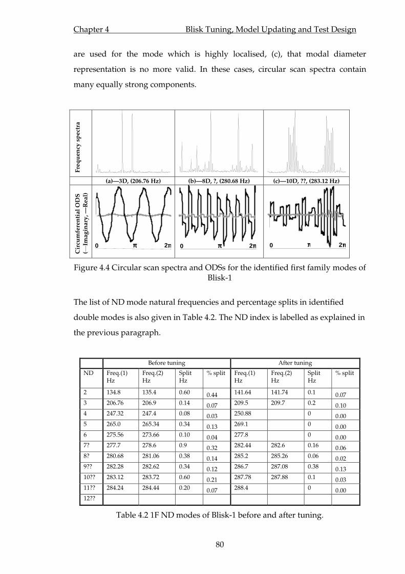
Chapter 4 Blisk Tuning, Model Updating and Test Design
80
are used for the mode which is highly localised, (c), that modal diameter
representation is no more valid. In these cases, circular scan spectra contain
many equally strong components.
Fre
qu
ency
sp
ect
ra
(a)—3D, (206.76 Hz) (b)—8D, ?, (280.68 Hz) (c)—10D, ??, (283.12 Hz)
Cir
cum
fere
nti
al
OD
S
(—Im
ag
ina
ry,
—R
ea
l)
Figure 4.4 Circular scan spectra and ODSs for the identified first family modes of Blisk-1
The list of ND mode natural frequencies and percentage splits in identified
double modes is also given in Table 4.2. The ND index is labelled as explained in
the previous paragraph.
Before tuning After tuning
ND Freq.(1) Hz
Freq.(2) Hz
Split Hz
% split Freq.(1) Hz
Freq.(2) Hz
Split Hz
% split
2 134.8 135.4 0.60 0.44 141.64 141.74 0.1 0.07
3 206.76 206.9 0.14 0.07 209.5 209.7 0.2 0.10
4 247.32 247.4 0.08 0.03 250.88 0 0.00
5 265.0 265.34 0.34 0.13 269.1 0 0.00
6 275.56 273.66 0.10 0.04 277.8 0 0.00
7? 277.7 278.6 0.9 0.32 282.44 282.6 0.16 0.06
8? 280.68 281.06 0.38 0.14 285.2 285.26 0.06 0.02
9?? 282.28 282.62 0.34 0.12 286.7 287.08 0.38 0.13
10?? 283.12 283.72 0.60 0.21 287.78 287.88 0.1 0.03
11?? 284.24 284.44 0.20 0.07 288.4 0 0.00
12??
Table 4.2 1F ND modes of Blisk-1 before and after tuning.
ππππ 0 2ππππ ππππ 0 2ππππ ππππ 0 2ππππ
Chapter 4 Blisk Tuning, Model Updating and Test Design
81
Judging from Table 4.2, the tuned state of Blisk-1 has been reasonably improved,
compared with the “before tuning” state, with mode splits of less than 0.13%.
However, this has not been sufficient to yield regular (i.e., tuned) assembly
modes for the entire 1F family. Various aspects of tuning through individual
blades are explored through a systematic study on a lumped-parameter model
in Section 4.2.3 to find out the reasons behind this failure and to asses whether a
better tuned state could have been achieved.
In order to quantify the effects of an applied mistuning pattern, the reference
case to which the obtained results could be related must be known fairly
accurately. Since the inherent and significant mistuning present in the blisk was
not known, it was concluded that it would not serve as a suitable reference for
mistuning investigations. As a result, it was decided to have another blisk made
to be used for mistuning studies. Blisk-1, nevertheless, could be used in friction
damping experiments if the present mistuning was reasonably identified.
4.2.2 Blisk-2
Based on the experience gained with Blisk-1, the geometry of Blisk-2 was kept
simple and the manufacture was tightly controlled. Blisk-2 1F modes natural
frequencies were measured in the same way as for Blisk-1, and the measured
frequencies and identified ND numbers are given in Table 4.3. The impact
response spectra from which these frequencies were extracted are also given in
Figure 4.5. Despite the use of a considerably high frequency resolution (0.02 Hz),
only 2 and 11 ND modes are found to be split, by 0.3% and 0.02% respectively.
For all other modes, the separation in repeated modes could not be identified.
The double modes given in Table 4.3 could only be identified in different impact
tests (i.e., changing the input force location), therefore they are not apparent
from Figure 4.5.

Chapter 4 Blisk Tuning, Model Updating and Test Design
82
ND # 2 3 4 5 6 7 8 9 10 11 12
Freq 1 172.34 212.44 240.98 257.58 267.7 274.18 278.52 281.42 283.3 284.32 284.68
Freq 2 172.84 — — — — — — — — 384.38 —
% split 0.3 0 0 0 0 0 0 0 0 0.02 0
Table 4.3 Measured 1F Blisk-2 frequencies.
170 172 174 176
Am
plitu
de (
dB)
208 210 212 214 216Frequency (Hz)
235 240 245
255 256 257 258 259
Am
plitu
de (
dB)
266 268 270 272 274 276 278 281 282 283 284 285
Figure 4.5 Blisk-2 impact response spectra
Based on the circumferential ODSs, the as-delivered tuned state of Blisk-2 was
significantly superior to that of Blisk-1. However, the sensitivity of the applied
mistuning to present inherent mistuning, however small, needed to be
investigated so that the exact state of tune of Blisk-2 could be validated. To this
end, a test setup is devised in which a random mistuning pattern was applied to
the blisk and the ODS at platform level was measured by circular scanning LDV.
Then, this pattern was shifted around the blisk by three blades (45°) and the
ODSs are re-measured. The applied mistuning patterns are given in Table 4.4.
Blade # Pattern 1 (gr) Pattern 2 (gr) Blade # Pattern 1 (gr) Pattern 2 (gr)
1 0.87 2.01 13 1.80 2.24
2 1.87 2.23 14 1.80 2.77
3 0.87 2.65 15 1.74 0.87
4 2.37 0.87 16 2.58 1.80
5 1.85 1.87 17 2.51 1.80
6 1.87 0.87 18 2.62 1.74
7 2.72 2.37 19 1.50 2.58
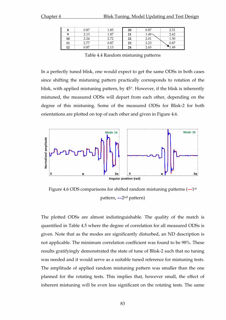
Chapter 4 Blisk Tuning, Model Updating and Test Design
83
8 0.87 1.85 20 0.87 2.51
9 2.13 1.87 21 1.49 2.62
10 2.24 2.72 22 2.01 1.50
11 2.77 0.87 23 2.23 0.87
12 0.87 2.13 24 2.65 1.49
Table 4.4 Random mistuning patterns
In a perfectly tuned blisk, one would expect to get the same ODSs in both cases
since shifting the mistuning pattern practically corresponds to rotation of the
blisk, with applied mistuning pattern, by 45°. However, if the blisk is inherently
mistuned, the measured ODSs will depart from each other, depending on the
degree of this mistuning. Some of the measured ODSs for Blisk-2 for both
orientations are plotted on top of each other and given in Figure 4.6.
Angular position (rad)
Nor
mal
ised
am
plitu
de
Mode 14 Mode 16
0 ππππ 2 ππππ 0 ππππ 2 ππππ
Figure 4.6 ODS comparisons for shifted random mistuning patterns (—1st
pattern, —2nd pattern)
The plotted ODSs are almost indistinguishable. The quality of the match is
quantified in Table 4.5 where the degree of correlation for all measured ODSs is
given. Note that as the modes are significantly disturbed, an ND description is
not applicable. The minimum correlation coefficient was found to be 98%. These
results gratifyingly demonstrated the state of tune of Blisk-2 such that no tuning
was needed and it would serve as a suitable tuned reference for mistuning tests.
The amplitude of applied random mistuning pattern was smaller than the one
planned for the rotating tests. This implies that, however small, the effect of
inherent mistuning will be even less significant on the rotating tests. The same

Chapter 4 Blisk Tuning, Model Updating and Test Design
84
test was applied to Blisk-1 as well, where considerable deviations in
corresponding ODSs from pattern to pattern were observed, as expected.
Mode #Freq (Hz)Pattern 1
Freq (Hz)Pattern 2
% freq. change% corr. coef.
1 165.22 165.60 0.23 99.46
2 167.20 166.90 -0.18 99.82
3 202.94 202.92 -0.01 99.40
4 203.86 203.86 0.00 99.39
5 229.32 229.32 0.00 99.16
6 230.16 230.18 0.01 98.83
7 243.72 243.70 -0.01 98.73
8 245.90 245.96 0.02 98.39
9 259.22 259.18 -0.02 99.44
10 260.90 260.90 0.00 98.55
11 262.82 262.86 0.02 99.16
12 265.34 265.34 0.00 98.72
13 266.50 266.60 0.04 98.19
14 267.14 267.18 0.01 99.70
15 271.34 271.34 0.00 99.75
16 273.18 273.24 0.02 99.23
Table 4.5 Correlation of randomly mistuned Blisk-2 ODSs
The percentage changes in the frequencies of first two modes given in Table 4.5
are an order of magnitude larger than those of the other modes. This might be
explained by the sensitivity of these frequencies to disk fixing, more than the
degree of inherent mistuning, as the ODSs correlate excellently.
4.2.3 On blisk tuning through individual blade frequencies
The experience with Blisk-1 demonstrated that the common practice of tuning 1F
blade-alone natural frequencies was not enough even to tune the 1F assembly
modes of the blisk satisfactorily. Although the 1F blade-alone natural
frequencies were matched to a degree, it is certain that the symmetry of the
system would have been improved had more than one blade-alone natural
frequencies been made identical. There are a number of reasons for this. First, it
is anticipated that the way in which changes were made to tune the 1F blade-
alone natural frequencies plays an important role. Considering an isolated blade
as a single DOF system represented by a lumped mass, m , and a stiffness, k ,
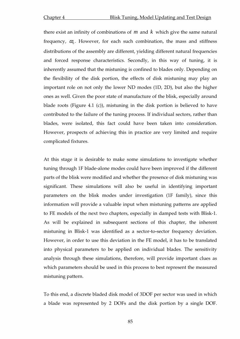
Chapter 4 Blisk Tuning, Model Updating and Test Design
85
there exist an infinity of combinations of m and k which give the same natural
frequency, 0ω . However, for each such combination, the mass and stiffness
distributions of the assembly are different, yielding different natural frequencies
and forced response characteristics. Secondly, in this way of tuning, it is
inherently assumed that the mistuning is confined to blades only. Depending on
the flexibility of the disk portion, the effects of disk mistuning may play an
important role on not only the lower ND modes (1D, 2D), but also the higher
ones as well. Given the poor state of manufacture of the blisk, especially around
blade roots (Figure 4.1 (c)), mistuning in the disk portion is believed to have
contributed to the failure of the tuning process. If individual sectors, rather than
blades, were isolated, this fact could have been taken into consideration.
However, prospects of achieving this in practice are very limited and require
complicated fixtures.
At this stage it is desirable to make some simulations to investigate whether
tuning through 1F blade-alone modes could have been improved if the different
parts of the blisk were modified and whether the presence of disk mistuning was
significant. These simulations will also be useful in identifying important
parameters on the blisk modes under investigation (1F family), since this
information will provide a valuable input when mistuning patterns are applied
to FE models of the next two chapters, especially in damped tests with Blisk-1.
As will be explained in subsequent sections of this chapter, the inherent
mistuning in Blisk-1 was identified as a sector-to-sector frequency deviation.
However, in order to use this deviation in the FE model, it has to be translated
into physical parameters to be applied on individual blades. The sensitivity
analysis through these simulations, therefore, will provide important clues as
which parameters should be used in this process to best represent the measured
mistuning pattern.
To this end, a discrete bladed disk model of 3DOF per sector was used in which
a blade was represented by 2 DOFs and the disk portion by a single DOF.
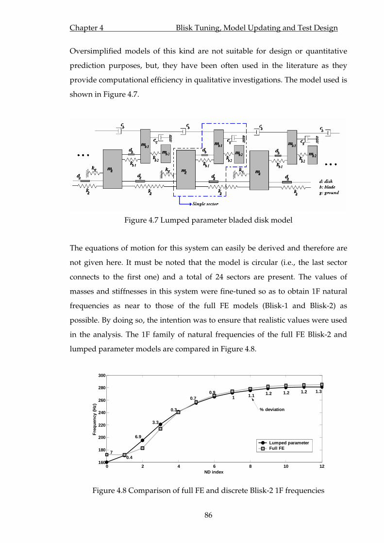
Chapter 4 Blisk Tuning, Model Updating and Test Design
86
Oversimplified models of this kind are not suitable for design or quantitative
prediction purposes, but, they have been often used in the literature as they
provide computational efficiency in qualitative investigations. The model used is
shown in Figure 4.7.
Figure 4.7 Lumped parameter bladed disk model
The equations of motion for this system can easily be derived and therefore are
not given here. It must be noted that the model is circular (i.e., the last sector
connects to the first one) and a total of 24 sectors are present. The values of
masses and stiffnesses in this system were fine-tuned so as to obtain 1F natural
frequencies as near to those of the full FE models (Blisk-1 and Blisk-2) as
possible. By doing so, the intention was to ensure that realistic values were used
in the analysis. The 1F family of natural frequencies of the full FE Blisk-2 and
lumped parameter models are compared in Figure 4.8.
0 2 4 6 8 10 12160
180
200
220
240
260
280
300
ND index
Fre
quen
cy (H
z)
70.4
6.9
3.3
0.3
0.7 0.9
1 1.1 1.2 1.2 1.2 1.3
Lumped parameterFull FE
% deviation
Figure 4.8 Comparison of full FE and discrete Blisk-2 1F frequencies

Chapter 4 Blisk Tuning, Model Updating and Test Design
87
4.2.3.1 Simulation of Blisk-1 tuning
As mentioned before the as-delivered mistuned state of Blisk-1 was mainly the
result of stiffness deviations whereas the tuning was accomplished via mass
removal. Inspections on the real blisk revealed that the thicknesses at the blade-
disk junction showed significant variability. Although not on the same scale,
some variations were also observed in the disk thicknesses as well. Therefore,
the blisk was mistuned via 1bk and dk stiffness terms in the simulations and then
tuned through mass 2bm using an isolated blade model. A 2 DOF lumped
parameter model was manageably small enough to be manipulated
parametrically in a symbolic solver such as Maple. Therefore, deriving equations
for the eigenvalues and solving them for certain parameters yielded the desired
accuracy for cases where convergence was achieved. Here a maximum of 0.35%
deviation in 1F blade frequencies was sought as this was the accuracy achieved
in Blisk-1 tuning. The results given in Figure 4.9 (a) show a general trend of
reduction in mode splitting, indicating an improved state of tune. However, the
split in ND modes does not automatically signify an irregularity of the mode
shapes. Particularly for lower ND modes, the shapes may remain regular despite
significant natural frequency splits in double modes since the modal density is
relatively low around these modes. The regularity of the mode shapes was
checked by Fourier analysis. The harmonic contents of a few tuned and
mistuned modes are given in Figure 4.9 (b) to (f). For a regular n ND mode of an
N -bladed blisk, Fourier analysis will yield significant n , N n− , N n+ etc
harmonics and negligible amplitudes for the rest (note that the amplitudes of
these harmonics will not necessarily be zero since the mode shape is defined by
only 24 discrete points). However, when the modes are irregular (i.e., mistuned),
additional non-trivial harmonics will show up depending on the degree of
irregularity. In this particular case, 7 ND and higher modes are clearly mistuned
as is evident from Figure 4.9. The irregularities in the modes with up to 8ND are
reasonably removed by adjusting the blade tip masses. However, as for the
Blisk-1 case, the higher ND modes were less regular and exhibited mode

Chapter 4 Blisk Tuning, Model Updating and Test Design
88
localisation which manifested itself in the form of non-trivial additional
harmonics.
1 2 3 4 5 6 7 8 9 100
0.1
0.2
0.3
0.4
0.5
ND Index
% S
plit
x 10
0
0 2 4 6 8 10 12 0 2 4 6 8 10 12
0 2 4 6 8 10 12 0 2 4 6 8 10 12
MistunedTuned
0 2 4 6 8 10 12
Mode # 18 (9-D)
Mode # 22 (11-D)
Mode # 24 (12-D)
Mode # 6(3-D)
Mode # 14 (7-D)
Nor
mal
ised
am
plitu
de
Harmonics
Harmonics
Nor
mal
ised
am
plitu
de
Figure 4.9 Blisk-1 tuning simulation
In the tuning process illustrated in Figure 4.9, all the individual 1F blade
frequencies were brought up to the level of the highest frequency blade as this
was the case in the real tuning of Blisk-1. However, aiming at the mean value of
the frequencies would be preferred, whenever possible. Simulations with this
particular model showed that, although not significantly different, a better state
of tune can be achieved this way. Also, it is desirable as it causes the least
disruption to individual blades.
The target error for blade-alone natural frequencies is reduced systematically
down to 0.0001% to see whether an improved tuned state was possible if blade-
alone frequencies were literally identical. The performed simulations showed an
overall decreasing split in some of the modes although no clear correlation
between increasing accuracy and the split in modes was evident. Fourier
analysis of the mode shapes showed similar results for the irregularity of the
modes. The results obtained for the 12ND mode are given in Figure 4.10 (note

Chapter 4 Blisk Tuning, Model Updating and Test Design
89
that only the 7-12 harmonics are shown as the 0-6 harmonics are almost zero).
Despite the drastic enhancement of the accuracy, the gain in terms of increased
tuned state has not been significant.
7 8 9 10 11 12ND Index
Nor
mal
ised
am
plitu
des
0.35 0.3 0.25 0.2 0.15 0.1 0.05 0.0010.0001
mode # 24(12-D)
% Error
Figure 4.10 12ND mode’s harmonics variation with increased accuracy in 1F
blade alone modes
The same procedure was repeated for a case in which the disk portion was
“perfectly” tuned (i.e., mistuned via 1bk and tuned via 2bm ) to demonstrate the
effect of disk mistuning. The accuracy of matching individual blade frequencies
was again set at 0.35%. Significantly better results are obtained for lower ND
modes, as expected, in terms of mode splits. Despite slight improvement,
however, the existence of irregularities in higher modes has not been possible to
eliminate.
In the light of the findings of the above analysis, it can be concluded that,
although the minimisation of variation in 1F blade-alone frequencies and the
inclusion of the effects of the disk portion’s mistuning might have resulted in a
better tuned state in Blisk-1, it would not be possible to tune the blisk
satisfactorily even if the adverse consequences of these effects were minimised.

Chapter 4 Blisk Tuning, Model Updating and Test Design
90
4.2.3.2 Tuning through various parameters
In this section simulations are presented where various parameters are used for
mistuning and subsequently tuning of the blisk. By doing so it is aimed at
identification of the sensitivity of the blisk tuning to various parameters and also
to see if, for a given mistuning pattern, a better combination for tuning of the
blisk existed when 1F blade alone frequencies were matched. Initially, mistuning
was introduced via 1bk stiffness element. Later, some other cases in which mass
mistuning and tuning through several parameters were also considered. The list
of cases studied is given in Table 4.6.
Mistuned via Tuned via
Case 1bk 2bk dk 1bm 2bm dm 1bk 2bk dk 1bm 2bm dm
1
2
3
4
5
6
7
8
9
10
Table 4.6 Mistuning/tuning test configuration
In all these cases, the 1F blade-alone frequencies are set to the same value of 300
Hz with an error of less than 0.0001%. The results, in the form of the natural
frequency split in the double modes corresponding to first four cases, are given
in Figure 4.11.
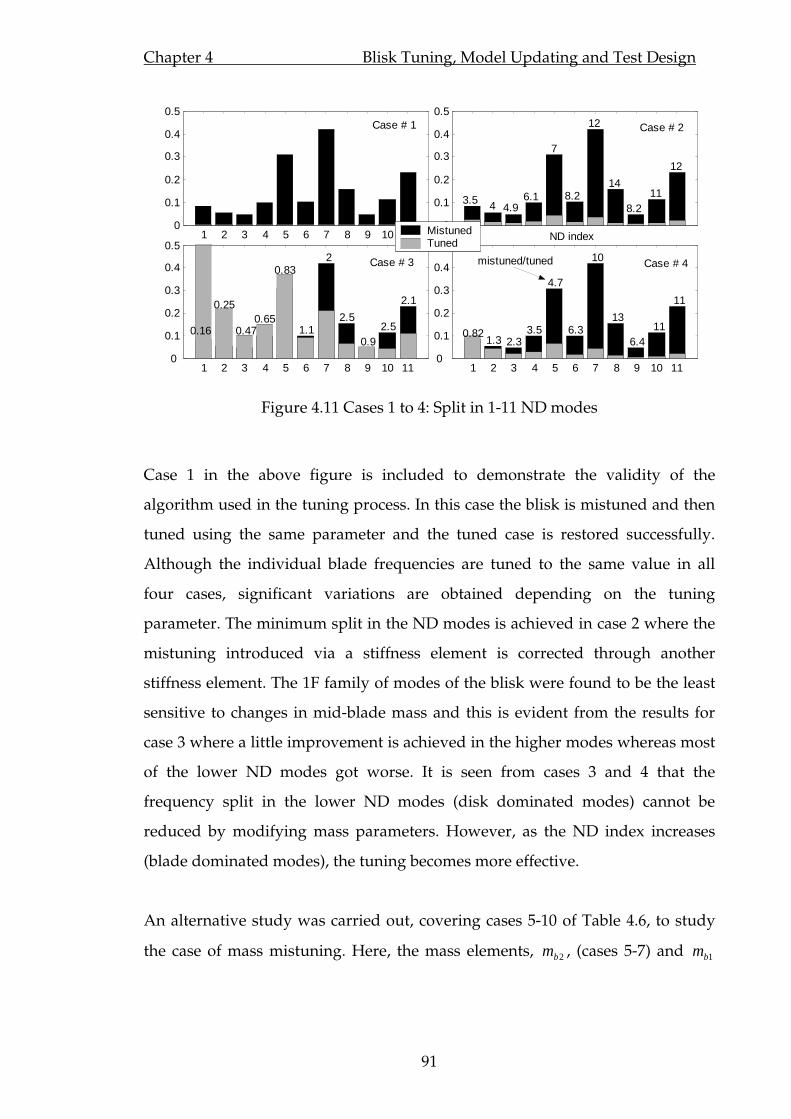
Chapter 4 Blisk Tuning, Model Updating and Test Design
91
1 2 3 4 5 6 7 8 9 10 110
0.1
0.2
0.3
0.4
0.5
0
0.1
0.2
0.3
0.4
0.5
3.5 4 4.96.1
7
8.2
12
14
8.2 11
12
ND index
1 2 3 4 5 6 7 8 9 10 110
0.1
0.2
0.3
0.4
0.5
0.16
0.25
0.470.65
0.83
1.1
2
2.5
0.9 2.5
2.1
1 2 3 4 5 6 7 8 9 10 110
0.1
0.2
0.3
0.4
0.5
0.82 1.3 2.3
3.5
4.7
6.3
10
13
6.4 11
11
MistunedTuned
Case # 1
Case # 3
Case # 2
Case # 4 mistuned/tuned
Figure 4.11 Cases 1 to 4: Split in 1-11 ND modes
Case 1 in the above figure is included to demonstrate the validity of the
algorithm used in the tuning process. In this case the blisk is mistuned and then
tuned using the same parameter and the tuned case is restored successfully.
Although the individual blade frequencies are tuned to the same value in all
four cases, significant variations are obtained depending on the tuning
parameter. The minimum split in the ND modes is achieved in case 2 where the
mistuning introduced via a stiffness element is corrected through another
stiffness element. The 1F family of modes of the blisk were found to be the least
sensitive to changes in mid-blade mass and this is evident from the results for
case 3 where a little improvement is achieved in the higher modes whereas most
of the lower ND modes got worse. It is seen from cases 3 and 4 that the
frequency split in the lower ND modes (disk dominated modes) cannot be
reduced by modifying mass parameters. However, as the ND index increases
(blade dominated modes), the tuning becomes more effective.
An alternative study was carried out, covering cases 5-10 of Table 4.6, to study
the case of mass mistuning. Here, the mass elements, 2bm , (cases 5-7) and 1bm

Chapter 4 Blisk Tuning, Model Updating and Test Design
92
(cases 8-10) were mistuned in turn. The results for these cases are given in Figure
4.12.
1 2 3 4 5 6 7 8 9 10 110
0.2
0.4
0.6
0.8
0
0.2
0.4
0.6
0.8
ND Index
% S
plit
x 10
0
1 2 3 4 5 6 7 8 9 10 110
0.2
0.4
0.6
0.8
1 2 3 4 5 6 7 8 9 10 110
0.05
0.1
0.15
0.2
1 2 3 4 5 6 7 8 9 10 110
0.05
0.1
0.15
0.2
1 2 3 4 5 6 7 8 9 10 110
MistunedTuned
Case 5 Case 6 Case 7
Case 8 Case 9 Case 10
Figure 4.12 Mass mistuning corrected through mass and stiffness elements
In all presented cases, 1F blade frequencies were brought to the same value and
in all cases the blisk characteristics achieved were different. Despite
improvements in some cases, none of the configurations were effective enough
to tune all the modes in the 1F family. In fact, there are a large number of
combinations of the stiffness and mass elements of an isolated blade which give
the same 1F frequency. Therefore, matching only this natural frequency will
result in different stiffness and mass distributions across the blisk, producing the
variability obtained in the above analysis. In order to improve the tuned state of
a blisk satisfactorily, a number of blade-alone natural frequencies may have to be
matched. This will limit the mass-stiffness combinations yielding these natural
frequencies. The efficiency of matching more than one blade alone frequency is
discussed in the next section. However, in cases where only one natural
frequency is to be matched, efforts should be made to identify the most sensitive
parameters so that the effectiveness of the tuning can be maximised. In an ideal
case, when the mistuning distribution is known precisely, corrections through
mistuned parameters will yield the desired tuned state. However, in general, the
mistuning patterns are not known. Additionally, it may not be possible to
modify those which are parameters responsible for mistuning in the direction
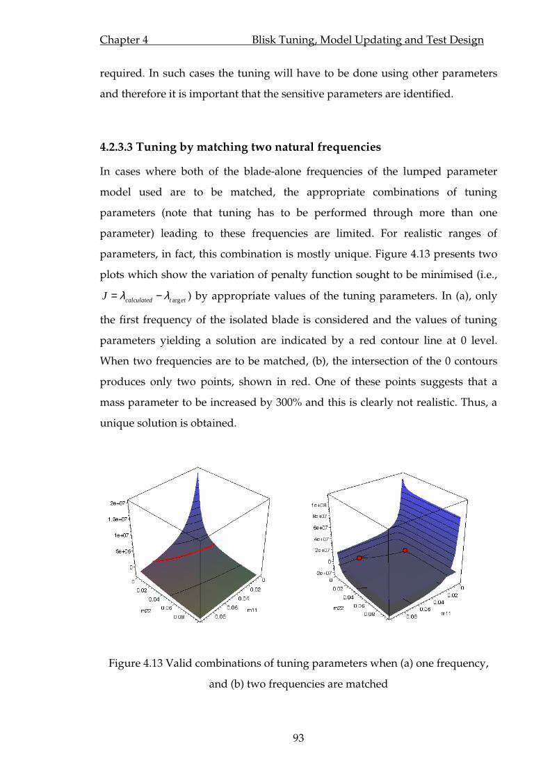
Chapter 4 Blisk Tuning, Model Updating and Test Design
93
required. In such cases the tuning will have to be done using other parameters
and therefore it is important that the sensitive parameters are identified.
4.2.3.3 Tuning by matching two natural frequencies
In cases where both of the blade-alone frequencies of the lumped parameter
model used are to be matched, the appropriate combinations of tuning
parameters (note that tuning has to be performed through more than one
parameter) leading to these frequencies are limited. For realistic ranges of
parameters, in fact, this combination is mostly unique. Figure 4.13 presents two
plots which show the variation of penalty function sought to be minimised (i.e.,
argcalculated t etJ λ λ= − ) by appropriate values of the tuning parameters. In (a), only
the first frequency of the isolated blade is considered and the values of tuning
parameters yielding a solution are indicated by a red contour line at 0 level.
When two frequencies are to be matched, (b), the intersection of the 0 contours
produces only two points, shown in red. One of these points suggests that a
mass parameter to be increased by 300% and this is clearly not realistic. Thus, a
unique solution is obtained.
Figure 4.13 Valid combinations of tuning parameters when (a) one frequency,
and (b) two frequencies are matched

Chapter 4 Blisk Tuning, Model Updating and Test Design
94
A table of cases analysed is given in Table 4.7. The blade root stiffness was
mistuned in all cases and the same blade mistuning pattern was maintained. In
the first three cases, the first blade-alone frequency was tuned to be compared
with the cases 3-6 where both of the blade-alone natural frequencies were tuned.
All the frequencies were brought literally to the same level (matched up to 12
significant digits).
Mistuned through Tuned through
Case 1bk 2bk 1bm 2bm 1bk 2bk 1bm 2bm
# of matched
frequencies
1 1
2 1
3 1
4 2
5 2
6 2
Table 4.7 Mistuning/tuning test configuration
The results obtained are shown in Figure 4.14. Depending on the combination of
parameters used to match both of the blade alone frequencies, significantly
different results were obtained. The best tuned reference case was achieved in
case 5 where the split in all ND modes was substantially reduced. The harmonic
content of the modes of this case exhibited clear components, corresponding to
the ND indices. Cases involving tuning through mid-blade mass 1bm yielded the
poorest results. Interestingly, the cases 1 and 3, where only the first blade-alone
natural frequencies were matched, produced, in general, relatively better results
compared to the cases 4 and 6 where both of the blade-alone natural frequencies
were matched.

Chapter 4 Blisk Tuning, Model Updating and Test Design
95
1 2 3 4 5 6 7 8 9 10 110
0.1
0.2
0.3
0.4
0.5
Nodal diamter index
% S
plit
MistunedCase 1Case 2Case 3Case 4Case 5Case 6
Figure 4.14 The comparison of cases given in Table 4.7.
4.2.3.4 Concluding remarks
It has been demonstrated through various virtual tests that the tuned state of a
blisk obtained by adjusting 1F blade-alone natural frequencies, no matter how
accurate the frequencies are matched, cannot be improved beyond a certain
accuracy. However, depending on the desired level of accuracy, some
parameters give substantially better results than others. In fact, the simulations
showed that, tuning through some parameters might even worsen the tuned
state. Therefore, before a tuning process is undertaken, it is useful to perform
preliminary simulations on a numerical model to identify the most effective
parameters.
The tuned state of the blisk has been sought to be improved by matching the
natural frequencies of the both, in-phase and out-of-phase, blade-alone modes of
the model used. With proper selection of tuning parameters it has been possible
to obtain a substantially better tune state compared to the cases where only 1F
blade frequencies were matched. However, it has been demonstrated that
matching both of the frequencies does not automatically produce the desired
tuned case. Though both blade frequencies were matched, some cases produced
inferior results. Therefore, the selection of proper tuning parameters is as
effective a factor as the number of matching frequencies. In fact, in a tuning

Chapter 4 Blisk Tuning, Model Updating and Test Design
96
process, attempts are made to enhance the dynamic properties of an assembly by
using a sub model of smaller size (e.g. an isolated blade) and different boundary
conditions. When the sensitivities of the natural frequencies of the sub model to
the tuning parameter are considerably different to those of the assembly
frequencies of interest, the tuning process may not lead to an improved tuned
state.
4.3 Model Updating
Up to this point, we have presented computed and measured blisk
characteristics separately. In a given design-to-manufacture process, though, the
characteristics of a machined test piece are inevitably different from those of the
design model. This might be either due to variations in dimensions resulting
from manufacturing tolerances or different material properties, or, in general,
due to both. The bladed disks introduced in the previous section are no
exception and a systematic approach is needed to reconcile the measured and
predicted properties. For this purpose, two techniques, inverse eigensensitivity
(IES) and so-called Fundamental Mode of Mistuning-Identification (FMM ID)
methods, have been used at various stages of updating of Blisk-1 and Blisk-2 FE
models.
4.3.1 Inverse eigensensitivity method
The inverse eigensensitivity method, [85-86], is one of the most commonly-used
FE model updating techniques in which either eigenvalues and/or eigenvectors
of the system are sought to be brought closer to the reference values (generally
measured data) by making appropriate changes to the updating parameters
based on the sensitivity of the system mass and stiffness matricies to these
updating parameters. The method employed in this study uses only the
eigenvalues in the updating process and therefore the Inverse Eigenvalue
Sensitivity (IES) method is employed.

Chapter 4 Blisk Tuning, Model Updating and Test Design
97
The ultimate goal of this method is to minimise the distance between the
measured and current model eigenvalues. Often an objective function of the
following form is used for the minimisation process:
2( )J p z= ∆ (4.1)
Where ( )FE refz λ λ∆ = − , and refλ represents the vector of measured eigenvalues
and FEλ the current values of the corresponding estimated eigenvalues. As the
penalty functions are generally nonlinear functions of updating parameters, they
are usually represented by truncated Taylor series. Representing FEλ as a
function of updating parameters, p , and expanding with respect to linearisation
point 0p p= and keeping only the 1st term gives
( )200( )J p z S pδ≅ ∆ + (4.2)
where the first term in the brackets represents the difference between measured
and calculated eigenvalues at the linearisation point, 0
FE
Sp
λ∂=∂
is the vector
containing the sensitivities of the eigenvalues to updating parameters and pδ is
the vector of increments to updating parameters which the updating process
seeks to obtain. The values of updating parameters can be found by partial
differentiation and then equating Equation (4.2) to zero. After some
manipulations, the updating equation in matrix form can be found as follows:
[ ] 0S p zλ δ = ∆ (4.3)
Here, pδ is the vector of changes in updating parameters to be calculated and
[ ]Sλ is the sensitivity matrix containing first derivatives of the eigenvalues with
respect to updating parameters. These sensitivities are calculated from the
structural eigenvalue problem of the form;
[ ] [ ] , 1..r r rK M r mφ λ φ= = (4.4)
Chapter 4 Blisk Tuning, Model Updating and Test Design
98
where K and M are the system stiffness and mass matricies. rλ and rφ are the
eigenvalue and mass normalised eigenvector of the rth mode. Differentiating
Equation (4.4) with respect to an updating parameter, rp , yields;
[ ] [ ] [ ] [ ] [ ]
0r r rr r r r r
r r r r r
K MK M M
p p p p p
φ λ φφ φ λ φ λ∂ ∂∂ ∂ ∂+ − − − =∂ ∂ ∂ ∂ ∂
(4.5)
Premultiplying Equation (4.5) by Trφ , rearranging and substituting
[ ] 1T
r rMφ φ = and [ ] [ ] 0T T
r r rK Mφ λ φ− = , the formula for eigenvalue
sensitivity can be obtained as,
[ ] [ ] Trr r r
r r r
K M
p p p
λ φ λ φ ∂ ∂∂ = − ∂ ∂ ∂
. (4.6)
Therefore sensitivity of an eigenvalue to updating parameters can be calculated
from that eigenvalue and the corresponding eigenvector. Applying Equation
(4.6) for all updating parameters, the sensitivity matrix [ ]Sλ of equation (4.3) can
be formed. Generally the penalty functions are non-linear function of updating
parameters therefore the solution of these equations require an iterative process
to be employed. In general the computed eigenvalues of the updating process
are weighted by some weighting factors to reflect the variation in the accuracy of
their measurements. In this case the data known to be more accurate is given
more weight in calculations.
4.3.2 FMM ID method
The Fundamental Mistuning Model– Identification (FMM ID) is a method of
mistuning identification proposed in [28]. It is based on the Fundamental
Mistuning Model (FMM) given in [13] where a highly reduced, 1 DOF per sector,
model of a bladed disk is used to predict the forced response for an isolated
family of modes. The FMM ID uses vibratory response measurements of a whole
bladed disk to work out existing mistuning on a sector to sector frequency
deviation basis. As it uses system modes and natural frequencies in analysis,
means that it is particularly suitable for integrally machined bladed disks (i.e.

Chapter 4 Blisk Tuning, Model Updating and Test Design
99
blisks). The fact that mistuning is identified for a cyclically symmetric sector,
disk mistuning as well as blade mistuning can be accounted for. This feature is
of particular importance for Blisk-1 since the inherent mistuning in this test piece
is not known and non-negligible. Meaningful predictions using this blisk will
only be obtained once the asymmetry is accounted for.
Details of the theory of the method can be found in abovementioned references.
A brief description of the underlying equations is summarised as follows. The
FMM modal equation upon which the theory of FMM ID is based, is given in
[28] as:
[ ] [ ] [ ]( ) 2 22 jT T T j jω Ω + Ω Ω Ω Β = Β (4.7)
where [ ]TΩ is a diagonal matrix of tuned system frequencies, Ω is a matrix
containing the discrete Fourier transforms of the sector frequency deviations,
each row of which is identical but shifted circularly. The eigenvector of Equation
(4.7), j
Β , contains the weighting factors that describe a mistuned mode as a
sum of tuned system modes in the form 1
0
NT
j j mmm
ϕ φ−
=
= Β where Tmφ is the mth
tuned mode shape and jmΒ is the corresponding weighting factor.
In Equation (4.7) the mistuning pattern is provided and the resulting mistuned
mode shapes and frequencies are calculated. The main idea of FMM ID is to
invert the FMM equation such that when mistuned modes and frequencies are
known, the individual blade mistuning pattern could be extracted as the
deviation of sector frequencies. The sector frequency of a particular sector used
here is calculated by mistuning all the sectors of the bladed disk in the same way
(i.e. by obtaining a new tuned system) and then calculating the mean ND mode
(i.e., 6ND mode in the case of a 24-blade bladed disk) of this system. The same is
repeated for all the mistuned sectors and the deviation of calculated mean ND
modes is taken as the mistuning pattern and defined as sector frequency
deviation.

Chapter 4 Blisk Tuning, Model Updating and Test Design
100
Two mistuning identification methods are proposed:
(i) basic FMM ID: where information of tuned mode shapes and frequencies is
expected to be provided (usually from FE). The mistuning identification in this
case is carried out through following equation:
[ ] [ ]( ) [ ] [ ]( ) 1 222 TjT j j
Iω ω−
= Ω Γ − Ω Β (4.8)
Where the inverse DFT of vector ω gives the sector frequency deviation (i.e.,
mistuning), matrix [ ] jΓ is formed by scaling the weighting factors given in
jΒ
by corresponding eigenvalues given in TΩ on an element by element basis. Each
row of this matrix is again identical but circularly shifted by one element in each
row. Equation (4.8) requires only one mode and the corresponding natural
frequency to work out the mistuning. Therefore errors in the measurements are
directly reflected on the identified mistuning pattern. In order to minimise the
effects of measurement errors, this equation is formed for several measured
modes for the modes of the family of interest and the resulting assembly of
equations is solved via a least squares fit as it cannot be solved by direct inverse
due to its over-determined nature.
(ii) advanced FMM ID: where only the experimentally-identified mistuned
natural frequencies and mode shapes of the bladed disk are needed. In this case
an estimation of the tuned bladed disk natural frequencies, as well as the
mistuning pattern, is returned. The equation of mistuning identification in this
case is given as:
[ ] [ ] [ ] 22 jj T j j
λω
ω Ρ Ω Γ = Β where
0
1
1
j
j
jn
j
j
Β
Β
Β
Β
Ρ =
(4.9)
Here, the given [ ] jΡ matrix is formed for a bladed disk with an even number of
blades. A similar one can be constructed when this number is odd. λ is the
vector of natural frequencies corresponding to identified tune case and, again,
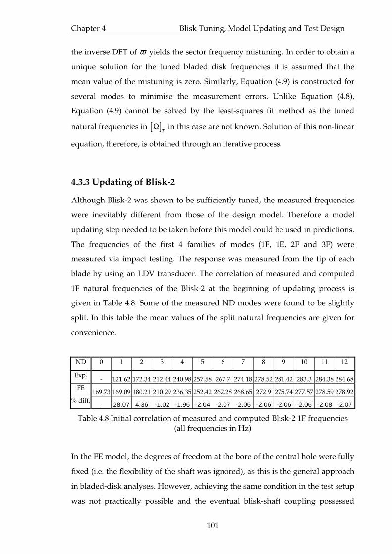
Chapter 4 Blisk Tuning, Model Updating and Test Design
101
the inverse DFT of ω yields the sector frequency mistuning. In order to obtain a
unique solution for the tuned bladed disk frequencies it is assumed that the
mean value of the mistuning is zero. Similarly, Equation (4.9) is constructed for
several modes to minimise the measurement errors. Unlike Equation (4.8),
Equation (4.9) cannot be solved by the least-squares fit method as the tuned
natural frequencies in [ ]TΩ in this case are not known. Solution of this non-linear
equation, therefore, is obtained through an iterative process.
4.3.3 Updating of Blisk-2
Although Blisk-2 was shown to be sufficiently tuned, the measured frequencies
were inevitably different from those of the design model. Therefore a model
updating step needed to be taken before this model could be used in predictions.
The frequencies of the first 4 families of modes (1F, 1E, 2F and 3F) were
measured via impact testing. The response was measured from the tip of each
blade by using an LDV transducer. The correlation of measured and computed
1F natural frequencies of the Blisk-2 at the beginning of updating process is
given in Table 4.8. Some of the measured ND modes were found to be slightly
split. In this table the mean values of the split natural frequencies are given for
convenience.
ND 0 1 2 3 4 5 6 7 8 9 10 11 12
Exp. - 121.62 172.34 212.44 240.98 257.58 267.7 274.18 278.52 281.42 283.3 284.38 284.68
FE 169.73 169.09 180.21 210.29 236.35 252.42 262.28 268.65 272.9 275.74 277.57 278.59 278.92
% diff. - 28.07 4.36 -1.02 -1.96 -2.04 -2.07 -2.06 -2.06 -2.06 -2.06 -2.08 -2.07
Table 4.8 Initial correlation of measured and computed Blisk-2 1F frequencies (all frequencies in Hz)
In the FE model, the degrees of freedom at the bore of the central hole were fully
fixed (i.e. the flexibility of the shaft was ignored), as this is the general approach
in bladed-disk analyses. However, achieving the same condition in the test setup
was not practically possible and the eventual blisk-shaft coupling possessed

Chapter 4 Blisk Tuning, Model Updating and Test Design
102
some degree of flexibility. The effect of this, was predominantly reflected on the
0-4ND mode frequencies, the 0 and 1 ND frequencies being particularly affected.
The contribution of the flexibility of the shaft on bladed-disk modes was studied
in [11] and similar findings were reported. However, as the lower ND modes
were not considered in the present study, the shaft flexibility was not included
in the FE analyses.
For most of the higher modes, the computed frequencies differed uniformly
from the measured ones by about 2%. Therefore, choosing an updating method
such as IES and including only these modes, the FE model could easily be
corrected to be a better representation of the real blisk. The mode shapes were
not included in the updating process as the blisk was found to be reasonably
tuned (i.e., having regular diametral mode shapes). Therefore, in theory,
selecting the material properties as updating parameters would suffice to
reconcile measured and computed frequencies. During the design phase,
material properties, density and modulus of elasticity, were taken to be
37800 /kg mρ = and 210E GPa= respectively. Only the modes with 5ND and
higher were included in the updating process as the lower ones were less
reliable due to the abovementioned reason. After a number of iterations, the IES
method converged to a reasonably tuned FE model with its 1F frequencies
fluctuating within ±0.1% (mostly around ±0.03%) of the measured values as
shown in Table 4.9. The correlations of 1E, 2F and 3F family natural frequencies
are also given in this table for which the deviations are less than 1%, 0.15% and
2.2%, respectively. Final density and modulus of elasticity values were obtained
as 37594.3 /kg mρ = and 207E GPa= .
1F 1E 2F 3F
ND Exp FE % Diff Exp FE % Diff Exp FE % Diff Exp FE % Diff
5 257.58 257.33 0.10 722.82 729.37 -0.91 1359.601357.50 0.15 2774.502713.76 2.19
6 267.70 267.54 0.06 723.18 728.74 -0.77 1477.401475.18 0.15 2802.502762.80 1.42
7 274.18 274.13 0.02 723.30 728.22 -0.68 1555.001553.16 0.12 2819.302789.31 1.06

Chapter 4 Blisk Tuning, Model Updating and Test Design
103
8 278.52 278.52 0.00 723.68 727.78 -0.57 1606.401604.90 0.09 2819.602805.64 0.50
9 281.42 281.47 -0.02 723.82 727.43 -0.50 1640.201639.03 0.07 2830.402816.28 0.50
10 283.30 283.36 -0.02 724.30 727.18 -0.40 1661.601660.66 0.06 2830.702823.11 0.27
11 284.38 284.41 -0.01 724.40 727.03 -0.36 1673.801672.65 0.07 2873.802826.95 1.63
12 284.68 284.76 -0.03 725.00 726.98 -0.27 1677.401676.50 0.05 2841.202828.19 0.46
Table 4.9 Blisk-2, 5-12ND 1F, 1E, 2F and 3F family natural frequencies, measured and updated (all frequencies in Hz)
The ODSs of the stationary Blisk-2 for the modes included in updating process
were also measured in the way described in Chapter 3 so that they could be
correlated with the updated FE model. Some of the 1F family modes are
compared in Figure 4.15. Spikes seen on experimental curves were due to
discontinuities at platform level (where the LDV signal drops to zero). Excellent
agreement was obtained not only for the lower ND modes but also for the higher
ones where the modes are very sensitive to mistuning due to the high modal
density. Based on the quality of correlation between measured and calculated
frequencies and ODSs, the Blisk-2 FE model was assumed to be updated and
could be used for prediction purposes.
-0.5
0
0.5
Rel
ativ
e am
plitu
de
-0.4
-0.2
0
0.2
0.4
Angular position (degree)
0 180 360-0.4
-0.2
0
0.2
0.4
0 180 360-0.4
-0.2
0
0.2
0.4
ExpFE Angular position (degree)
5D 6D
11D 12D
Figure 4.15 Correlation of measured and computed ODSs for 5, 6, 11 and 12D, 1F family modes
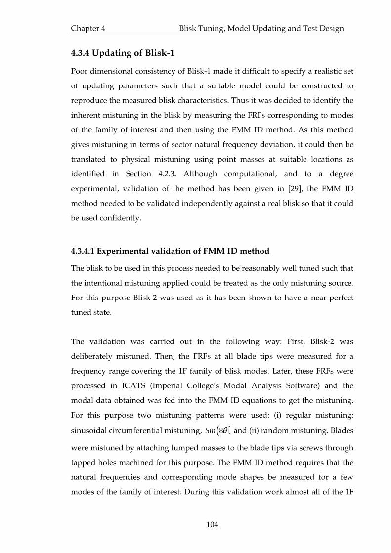
Chapter 4 Blisk Tuning, Model Updating and Test Design
104
4.3.4 Updating of Blisk-1
Poor dimensional consistency of Blisk-1 made it difficult to specify a realistic set
of updating parameters such that a suitable model could be constructed to
reproduce the measured blisk characteristics. Thus it was decided to identify the
inherent mistuning in the blisk by measuring the FRFs corresponding to modes
of the family of interest and then using the FMM ID method. As this method
gives mistuning in terms of sector natural frequency deviation, it could then be
translated to physical mistuning using point masses at suitable locations as
identified in Section 4.2.3. Although computational, and to a degree
experimental, validation of the method has been given in [29], the FMM ID
method needed to be validated independently against a real blisk so that it could
be used confidently.
4.3.4.1 Experimental validation of FMM ID method
The blisk to be used in this process needed to be reasonably well tuned such that
the intentional mistuning applied could be treated as the only mistuning source.
For this purpose Blisk-2 was used as it has been shown to have a near perfect
tuned state.
The validation was carried out in the following way: First, Blisk-2 was
deliberately mistuned. Then, the FRFs at all blade tips were measured for a
frequency range covering the 1F family of blisk modes. Later, these FRFs were
processed in ICATS (Imperial College’s Modal Analysis Software) and the
modal data obtained was fed into the FMM ID equations to get the mistuning.
For this purpose two mistuning patterns were used: (i) regular mistuning:
sinusoidal circumferential mistuning, ( )8Sin θ and (ii) random mistuning. Blades
were mistuned by attaching lumped masses to the blade tips via screws through
tapped holes machined for this purpose. The FMM ID method requires that the
natural frequencies and corresponding mode shapes be measured for a few
modes of the family of interest. During this validation work almost all of the 1F

Chapter 4 Blisk Tuning, Model Updating and Test Design
105
family modes were measured so that the applicability of the method could be
checked when various combinations of measured modes were used. The FRFs
were measured by applying a pseudo-random excitation through an
electromagnet and measuring the response at blade tips using an LDV beam
normal to the plane of the blisk. Since the FMM ID operated on the relative
amplitudes of response measurement locations at a given resonance, the
measured mode shapes did not need to be normalised by the actual applied
force magnitude but they were divided by the voltage input generated by the
power unit driving the electromagnet (Note that here it is assumed that the force
generated is proportional to the input voltage). Each mode shape contained 24
measurement points corresponding to deflections at the 24 blade tip locations.
As will be explained in the next chapter, the response prediction tools used
required that the mistuning pattern be expressed in terms of the frequency
variation of a sub-model, such as a blade clamped at the root. The applied mass
mistuning, therefore, was converted to blade frequency deviation so that a
consistent mistuning definition could be used. This was done by modelling a
single blade of Blisk-2. The geometry and the weight of the mistuning masses
were modelled as closely as possible and the 1F frequencies of all the blades
clamped at the root were computed. The percentage deviations of these
frequencies from those of the perfectly tuned blade were calculated to obtain the
actual frequency mistuning. Bearing in mind that the FMM ID method expresses
mistuning as sector frequency deviation (see Section 4.3.2 for the definition of
the sector frequency), further processing of the obtained mistuning is necessary
to get comparable results. Assuming the mistuning is confined to the blade,
which in this case it is, a sector frequency deviation simply differs from a blade
frequency deviation by a scaling factor. To obtain the appropriate scaling factor,
N/4 ND mode frequency (i.e., the reference ND mode FMM ID uses in
computations), N being the total number of sectors, of the perfectly tuned Blisk-2
was computed. Then, the blade modulus was changed uniformly to increase it's
frequency by 1%. Using this modulus for all blades N/4 ND mode frequency of

Chapter 4 Blisk Tuning, Model Updating and Test Design
106
the blisk was recalculated. The inverse of the percentage change in N/4
frequency in both cases, therefore, gave the scaling factor to obtain the blade
frequency deviation from the sector frequency deviation. The scaling factor for
Blisk-2 was found to be 1.11 so the output of FMM ID was multiplied by this
factor to obtain the blade frequency deviations.
The correlation between the applied mistuning pattern and the one identified
through the FMM ID Basic method is given in Figure 4.16. The tuned blisk
frequencies provided for mistuning identification were those of the updated
model given in the previous section. Overall, a very good match is obtained
between the two patterns with a correlation coefficient of 98.8%. The only
significant deviation observed was for blades 7 to 10. Here it must be noted that
the effectiveness of the mistuning prediction method relies totally on the
accuracy of the provided modal data. Since they possess repeated modes,
providing reliable modal data could be difficult for symmetric structures such as
bladed disks. In the case of these double modes being slightly split, identification
of mode shapes and frequencies requires very high frequency resolution which
may not be achievable, depending on the analyser used. Here, the prominent
deviations observed from Figure 4.16 are thought to be associated with this
feature of the blisk rather than the inefficiency of the identification tool. Note
that although mistuned, the blisk in this case is still symmetric and most of its
double modes (in fact, all but 8 and 4 ND modes) are only slightly split if at all.
2 4 6 8 10 12 14 16 18 20 22 24-20
-15
-10
-5
0
5
Blade #
Bla
de fr
eque
ncy
devi
atio
n (%
)
AppliedFMM-ID Basic
Figure 4.16 Correlation of applied and identified mistuning patterns - ( )8Sin θ
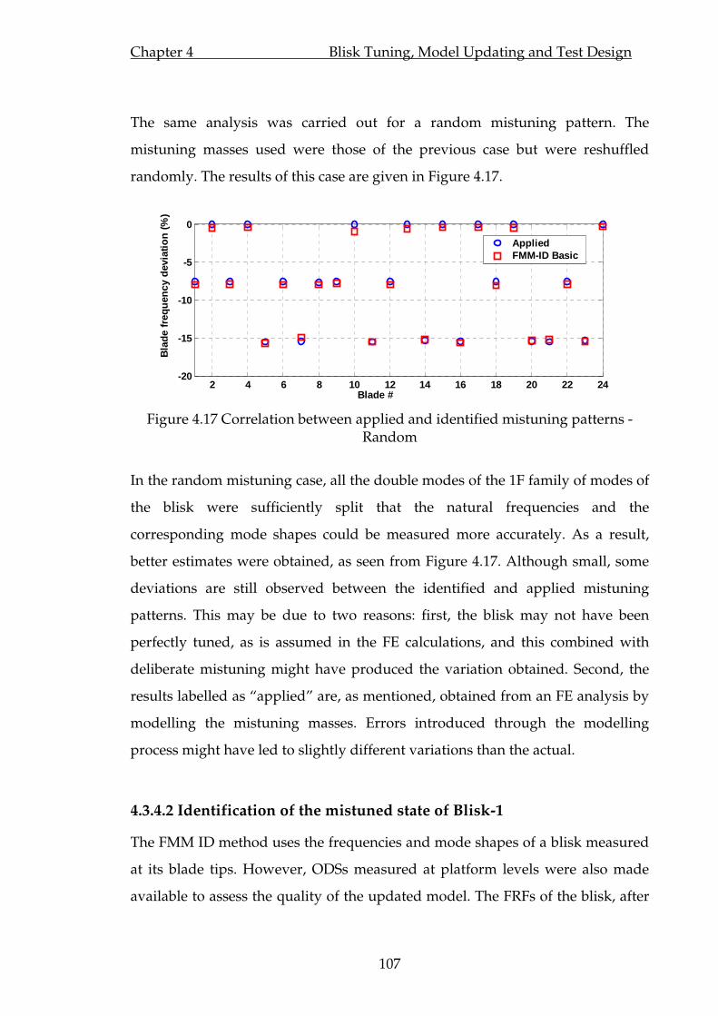
Chapter 4 Blisk Tuning, Model Updating and Test Design
107
The same analysis was carried out for a random mistuning pattern. The
mistuning masses used were those of the previous case but were reshuffled
randomly. The results of this case are given in Figure 4.17.
2 4 6 8 10 12 14 16 18 20 22 24-20
-15
-10
-5
0
Blade #
Bla
de fr
eque
ncy
devi
atio
n (%
)
AppliedFMM-ID Basic
Figure 4.17 Correlation between applied and identified mistuning patterns - Random
In the random mistuning case, all the double modes of the 1F family of modes of
the blisk were sufficiently split that the natural frequencies and the
corresponding mode shapes could be measured more accurately. As a result,
better estimates were obtained, as seen from Figure 4.17. Although small, some
deviations are still observed between the identified and applied mistuning
patterns. This may be due to two reasons: first, the blisk may not have been
perfectly tuned, as is assumed in the FE calculations, and this combined with
deliberate mistuning might have produced the variation obtained. Second, the
results labelled as “applied” are, as mentioned, obtained from an FE analysis by
modelling the mistuning masses. Errors introduced through the modelling
process might have led to slightly different variations than the actual.
4.3.4.2 Identification of the mistuned state of Blisk-1
The FMM ID method uses the frequencies and mode shapes of a blisk measured
at its blade tips. However, ODSs measured at platform levels were also made
available to assess the quality of the updated model. The FRFs of the blisk, after

Chapter 4 Blisk Tuning, Model Updating and Test Design
108
it was subjected to the tuning process given in Section 4.2.1, were measured in
the same way as the Blisk-2 measurements were conducted for FMM ID
validation. The blisk was clamped in the centre in the same way as it was to be
clamped in the rig. The natural frequencies and mode shapes were extracted
from measured FRFs by using ICATS software. The correlation between the
natural frequencies of the initial design and the measurements is given in Table
4.10. A sufficiently fine frequency resolution (0.008 Hz) was used in order to
make sure that split ND modes were identified accurately. AutoMAC between
the measured mode shapes was also checked and excellent orthogonality was
observed, as given in Table 4.10.
Experimental Computed 1F ND Freq1 (Hz) FE (Hz) Freq 2 (Hz)
% Difference
AutoMAC
0 102.58 NA 133.503 -30.15 1 29.42 29.802 117.474 -296.72 2 136.72 136.831 110.607 19.13 3 204.32 204.540 195.522 4.36 4 247.25 247.345 234.527 5.16 5 266.56 266.658 252.078 5.45 6 275.74 275.772 260.519 5.53 7 280.53 280.730 265.078 5.54 8 283.41 283.487 267.748 5.54 9 284.94 285.354 269.375 5.53
10 286.097 286.186 270.354 5.52 11 286.716 286.937 270.881 5.56 12 287.535 NA 271.048 5.73
0
0.1
0.2
0.3
0.4
0.5
0.6
0.7
0.8
0.9
1
10 12 14 16 18 20 22 24
10
12
14
16
18
20
22
24
Table 4.10 Correlation between initial FE and measured frequencies (--Frequencies used in IES method, --: modes used in mistuning identification)
Note that the experimental values given in this table are slightly different from
those given in Table 4.2. This is due to the integration of blade inserts. The
frequencies, in general, are lower. However, the split in the mode pairs and the
distortion of the mode shapes were unchanged. In fact, during the integration of
the blade inserts, efforts were made to improve the tuned state of the blisk by
arranging the blade inserts appropriately. However, little, if at all, improvement
was achieved. In the light of findings presented in Section 4.2.3, this was not

Chapter 4 Blisk Tuning, Model Updating and Test Design
109
surprising, since the assembly modes were found to be not very sensitive to
mass changes at the locations where the inserts were mounted.
As for the Blisk-2 case, the natural frequencies of the 0, 1 and 2-ND modes were
significantly lower than the predicted ones due to different boundary conditions
in the real test setup and the FE model. As for the 3-ND and higher modes, a
steady deviation of 4-6% was apparent. The fact that the deviation for these
modes was in the same direction (i.e., experimental frequencies were higher than
FE predicted ones), indicated that the overall material properties needed to be
adjusted. At first, it was sought to change the material properties such that the
percentage difference between the measured and computed frequencies
oscillated around zero. This could be done either through modifying the density
or elasticity modulus, or both, using the IES method.
When designing Blisk-1, the material properties, density and modulus of
elasticity, were assumed to be 37800 /kg mρ = and 210E GPa= , respectively.
These were used as updating parameters in the IES updating method. The 5ND
and higher modes were taken into account in the analysis as the lower modes
were known to be less accurate for other reasons. The reference frequency value
aimed at for each ND mode was the mean value of the corresponding split pair
measured. At the end of the updating process, the density and elastic modulus
were found to be; 37130 /kg mρ = and 215E GPa= . Using these values, the 1F
blisk natural frequencies (those with 5ND and higher) were brought within 0.6%
of the reference (i.e. measured) natural frequencies, as given in Table 4.11.
ND # 5 6 7 8 9 10 11 12
FE 266.78 275.71 280.53 283.36 285.08 286.12 286.68 286.85
Exp. (mean.) 266.61 275.76 280.63 283.45 285.15 286.14 286.83 287.54
% Difference -0.06 0.02 0.03 0.03 0.02 0.01 0.05 0.24
Table 4.11 Blisk-1 FE frequencies after updating via IES method

Chapter 4 Blisk Tuning, Model Updating and Test Design
110
Now that the 1F natural frequencies of the FE model were brought closer to the
actual values, the FMM ID Basic method could be used to identify the inherent
mistuning as a deviation from this tuned FE model. Again, only 5ND and higher
modes were used in the analysis. The mistuning pattern, obtained as a set of
sector frequency deviations, was again converted such that it could be expressed
in terms of the frequency deviation of the sub-model used. In the case of Blisk-1,
a cyclic sector is used as a sub-model and is clamped at the cyclic boundary faces
(faces on which cyclic symmetry boundary conditions are applied). The reason
for this was that the sector model would have the disc portion as well as the
blade and therefore it would be possible to include the effect of disc mistuning
too. The FE model calculations revealed that a scaling factor of 1.14 (i.e.
1.14xNat. Frequencies) needed to be used in the conversion. The deviation of the
clamped sector-alone 1F natural frequencies obtained using this scaling factor is
given in Figure 4.18.
2 4 6 8 10 12 14 16 18 20 22 24
-0.5
0
0.5
1
-0.03
0.24
0.04
-0.78
0.43
0.72
1.1
0.38
-0.39
-0.17 -0.06
-0.4
0.24
-0.26
-0.68
0.12
-0.56
-0.03
0.09
-0.25
-0.00
-0.24
0.01
0.14
Blade #
Sec
tor
freq
uenc
y de
viat
ion
(%)
Figure 4.18 Identified Blisk-1 mistuning in terms of clamped, sector-alone
frequency deviation
4.3.4.3 Verification of the mistuning pattern identified
The accuracy of the mistuned natural frequencies and the mode shapes
calculated using the pattern identified had to be checked against the measured
counterparts. This, eventually, would have to be done using the full Blisk-1 FE
model but some preliminary checks could be performed by using the 1 DOF

Chapter 4 Blisk Tuning, Model Updating and Test Design
111
sector model of the FMM method. To this end, the mistuning pattern was used
in Equation (4.7) and the mistuned mode shapes of the blisk were recalculated.
The correlation between the measured and calculated mode shapes is given in
Figure 4.19 (a). Another useful check was to use the FMM ID Advanced Method
(i.e. no tuned FE model data provided) to calculate the natural frequencies of the
tuned reference state from the mistuned mode shapes and frequencies. The
closeness of these tuned frequencies to the FE model frequencies used in the
FMM ID Basic Method would provide further confidence in the obtained result.
This comparison is given in Figure 4.19 (b). It is seen that the estimates for the 0-
4D modes are significantly higher. This can be explained by the fact that only the
5D and higher modes were included in the identification process. In this case,
the estimates for the excluded modes were worked out based on the amplitudes
of the components corresponding to these modes (i.e. spatial Fourier harmonics)
in the included ones. Better estimates for the natural frequencies of these modes
could be obtained by inclusion of their mode shapes in the process. Note that the
mistuning identification is not affected by the exclusion of these modes. A very
close match is obtained for included modes (i.e. 5D and up) indicating that the
mistuning obtained is reasonably accurate.
0 2 4 6 8 10 12100
150
200
250
300
ND index
Nat
ural
fre
quen
cies
(H
z)
FEFMM-ID Advanced
5 10 15
2
4
6
8
10
12
14
16
Measured mode #
FM
M I
D m
ode
#
0.1
0.2
0.3
0.4
0.5
0.6
0.7
0.8
0.9
(a) (b)
Figure 4.19 (a) Correlation between measured and FMM calculated mistuned modes, (b) Full FE model tuned frequencies vs. FMM ID Advance estimates
Good initial correlation obtained using the 1 DOF per sector model of the FMM
method was tested with the FE model of Blisk-1, as this model would be used in

Chapter 4 Blisk Tuning, Model Updating and Test Design
112
the analyses. The prediction tool to be used, which is to be validated in the
course of this study, was intended for response calculations only and did not
provide mode shapes. As a result, the mode shapes of Blisk-1 with applied
mistuning pattern needed to be calculated using a commercial FE package, such
as ANSYS. Since the cyclic sector analysis in this package was not applicable to
mistuned assemblies, a full FE model needed to be prepared so that the
mistuning could be applied. The easiest and most convenient way of converting
the identified frequency mistuning into physical mistuning was to modify each
sector’s Young’s modulus according to its frequency deviation. For example, if a
sector’s frequency deviation is +1%, one needs to multiply the Young’s modulus
of that sector by 1.012 ≅ 1.02. The fact that the mistuning identification method
operates on a 1 DOF sector model, means that representing the mistuning in this
way (i.e. uniform variation of a single parameter for each sector) yields a very
good approximation. Thus, the results obtained by this can be used as a
benchmark for the aptness of the model to be used in the prediction tool, in
which mistuning is required to be implemented by way of local mass and
stiffness adjustments. The correlation of the mode shapes of the full FE model
and those obtained from measurements is given in Figure 4.20 (a). The mean
value of MAC for the modes included in the mistuning identification was 86.5%,
indicating a successfully updated model. The natural frequencies of the full FE
model were also correlated with the measured ones. A maximum error of 0.7%
was observed for modes 8 and 9. However, in general, the calculated frequencies
were within 0.3% of the measured ones, as shown in Figure 4.20 (b). The larger
deviations in the lower natural frequencies, as mentioned, were due to the
flexibility of the disc clamping during measurements.

Chapter 4 Blisk Tuning, Model Updating and Test Design
113
0.1
0.2
0.3
0.4
0.5
0.6
0.7
0.8
0.9
8 10 12 14 16 18 20 22 24 8
10
12
14
16
18
20
22
24
Measured mode #
Ful
l FE
mod
e #
8 10 12 14 16 18 20 22 24240
250
260
270
280
290
Mode #
Nat
ural
fre
quen
cies
(H
z)
0.
7
0.7
0.1
9 0
.18
-0.0
41-0
.008 -
0.12
-0.
13 -0.
18-0
.098
-0.
15 -
0.21
-0.
24 -
0.16
-0.
27 -
0.2
0.0
96
MeasuredUpdated FE
% error
(a) (b)
Figure 4.20 (a) Correlation of the measured Blisk-1 modes with updated Blisk-1 FE model, (b) measured and computed Blisk-1 frequencies for 1F modes (8-24).
4.4 Test design
In a study seeking validation of numerical predictions, the selection of the
appropriate test configurations carries utmost importance in ensuring the
effectiveness and the usefulness of the measured data. This requires that a test
design phase be undertaken by performing a series of simulations in the
computer environment before any real tests are performed. The test design, or
test planning process in the classical modal analysis sense (i.e.,
drive/measurement point selection, suspension location etc.), is not applicable
in this study as the information of interest is either obvious (i.e.
drive/measurement points) or not applicable (i.e. suspension location).
Nevertheless, depending on the nature of the phenomena being validated, there
are a number of decisions the experimentalist is expected make, as explained in
following sections. The test planning presented here is oriented towards the
identification of test configurations (i.e. which EOs to measure, which mistuning
patterns to apply etc.). Although efforts are made to draw a definitive test plan
(including rotational speed ranges, necessary excitation forces, testing time etc.),
adjustments to these will inevitably be necessary in practice.
Chapter 4 Blisk Tuning, Model Updating and Test Design
114
4.4.1 Tuned and mistuned tests on Blisk-2
Validation of the mistuned bladed disk predictions were to be performed by
using the measurement results obtained on Blisk-2. It was decided from the
outset that only the 1F family of modes of the blisk should be considered. This
was thought appropriate since the employed LDV measurement technique
allowed only out-of-plane vibrations to be measured. It was also favourable
from the data acquisition point of view as lower sampling frequencies could be
used, thereby allowing manageably longer samples to be acquired for optimum
signal processing.
First, the tests to be conducted on the tuned blisk were planned. When testing a
bladed disk, it is necessary to map out the dynamic characteristics of the test
object (i.e. the locations of resonances). Experimentally, this is done through
construction of so-called z-mod plots. A z-mod plot is a surface plot, the height of
which (i.e. z -axis, hence the name z-mod) is determined by the vibration
response amplitude measured at a given point while x and y axes are defined
by the rotational speed and the vibration frequency, respectively. The colouring
of this surface is proportional to the height (i.e. vibration amplitude), so that the
resonances are easily observable. In order to make sure that such an
experimental graph is constructed as accurately as possible, the rig can be run
for the entire speed range with uniform and very small speed increments and
the vibration signal recorded at each speed step. However, using very small step
sizes is certainly not efficient as the valuable information and the need for fine
step sizes will only be necessary at around resonances. Therefore, having a prior
knowledge of the resonance map for the speed range of interest will be of
immense help in reducing the measurement time and data size without
compromising the completeness of the data. Based on the Campbell diagram of
Blisk-2 given in Chapter 3, and the reliable and safe working limits, the
operating speed limit of the test rig was chosen to be 4000 rev/min. A new
Campbell diagram using the updated Blisk-2 model was constructed for this
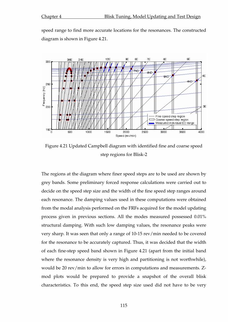
Chapter 4 Blisk Tuning, Model Updating and Test Design
115
speed range to find more accurate locations for the resonances. The constructed
diagram is shown in Figure 4.21.
Figure 4.21 Updated Campbell diagram with identified fine and coarse speed
step regions for Blisk-2
The regions at the diagram where finer speed steps are to be used are shown by
grey bands. Some preliminary forced response calculations were carried out to
decide on the speed step size and the width of the fine speed step ranges around
each resonance. The damping values used in these computations were obtained
from the modal analysis performed on the FRFs acquired for the model updating
process given in previous sections. All the modes measured possessed 0.01%
structural damping. With such low damping values, the resonance peaks were
very sharp. It was seen that only a range of 10-15 rev/min needed to be covered
for the resonance to be accurately captured. Thus, it was decided that the width
of each fine-step speed band shown in Figure 4.21 (apart from the initial band
where the resonance density is very high and partitioning is not worthwhile),
would be 20 rev/min to allow for errors in computations and measurements. Z-
mod plots would be prepared to provide a snapshot of the overall blisk
characteristics. To this end, the speed step size used did not have to be very

Chapter 4 Blisk Tuning, Model Updating and Test Design
116
small but fine enough to make sure that the resonances were captured.
Therefore, it was decided that 6-7 points should be measured for each fine-step
speed range. Thus, the fine speed step size was chosen to be 3 rev/min and all
other ranges were to be step-swept at 10 rev/min.
In practice the vibration response due to a particular EO excitation (or in some
cases a few) is generally of interest. In this study, however, it was decided to
measure the vibration response for all 1F family of modes excited within the
operating speed range of the rig (i.e. response to 4-12 EO excitations). Such a
wide range of measurements for a tuned blisk was affordable since measuring
only one blade for a particular EO excitation would suffice (i.e., in theory all
blades of a tuned blisk have the same vibration response). The lower end of the
EO range would, therefore, provide vibration data at relatively high rotational
speeds and the higher end of range would make vibration data at a relatively
high modal density region available. Unlike the z-mod plot measurements, EO
responses were to be measured for quantified comparisons with predictions.
Therefore, it was important that fine enough speed increments were used to
acquire accurate response curves. Recalling from Chapter 3, the minimum
attainable speed step with the motor controller employed was 1 rev/min.
However, preliminary response predictions using measured damping values
showed that in the immediate neighbourhood of resonance peaks, a step size of
0.05 rev/min would be needed to measure the resonance amplitudes accurately.
Achieving such fine speed increments would be very difficult in practice, if
indeed possible at all, and extremely expensive. Instead of comparing the whole
resonance curve, on the other hand, off-resonance regions (i.e. rising and falling
flanks of response curves), which could be constructed accurately using the
minimum achievable increment of 1 rev/min, could be used to correlate the
measurements and predictions. This is demonstrated on a computed response
curve shown in Figure 4.22. The red dots shown here represent likely
measurement points. It is seen that, bar the “region of uncertainty”, the response
curves can be measured reasonably well by using 1 rev/min steps. Based on

Chapter 4 Blisk Tuning, Model Updating and Test Design
117
Figure 4.22, a speed range of 100 rev/min, centred about the corresponding
resonance (EO-ND crossing), was chosen for each response curve, as indicated
by the blue portions of EO lines given in Figure 4.21.
Figure 4.22 Measurement plan for a particular EO response curve
With the completion of the test plan for tuned measurements, a mistuning test
programme was attempted next. To this end, the shapes and corresponding
amplitudes of mistuning patterns to be applied needed to be defined. Two
different sets of tests (stationary and rotating) were planned with a number of
mistuning patterns applied.
The purpose of the stationary tests was to experimentally determine the effect of
various types of mistuning patterns on blisk frequencies and mode shapes (or
more precisely, ODSs). The results of these tests would also provide preliminary
measurement data to assess the suitability of the FE model and the capabilities of
the prediction tool when the results are not yet complicated by the effects of
rotation. For this purpose, 3 mistuning patterns were chosen to be tested: (i)
single blade mistuning (SBM), which would cause all ND modes to split, (ii)
regular pattern mistuning, introducing a sinusoidal variation of blade
frequencies in the circumferential direction, which would result in only
particular modes splitting (see Section 2.2), and (iii) irregular (random)
mistuning, which would simulate a real case scenario. Mistuning was to be

Chapter 4 Blisk Tuning, Model Updating and Test Design
118
introduced using small masses attached to the blade tips. The amplitude of the
largest mass to be attached was chosen such that it would cause large enough
splits in the modes that they could be measured easily. Computations showed
that a mass of 1.7 gram would introduce a minimum frequency spit (SBM case)
of 0.2 Hz which could easily be measured with a 10Hz-span, 500-line zoom FFT.
The regular pattern was selected to be ( )12Sin θ⋅ , which required every other
blade to be mistuned by the same amount.
For the rotating mistuned tests, it was decided to use only two mistuning
patterns: regular and random. The SBM was not used as it would make the blisk
unbalanced and necessitate a balancing plane to be incorporated. It was thought
advisable to use the same mistuning masses for both patterns so as to minimise
the effort of preparing new ones. The regular pattern for the stationary tests was
clearly not suitable for this purpose as it contained masses of the same
amplitude. As a result, a ( )8Sin θ⋅ regular mistuning pattern was chosen to be
used. Fourier analysis performed on this pattern revealed the presence of strong
0th, 8th, 16th, and 24th harmonics which, recalling from Chapter 2, would cause the
0, 4, 8 and 12 ND modes to split. Noting that the 0 and 12 ND modes do not
occur in pairs, only the 4 and 8 ND mode pairs would split and the
corresponding resonances would be excited within the test rig’s working speed
range (0-4000 rev/min). Additionally, such a pattern contained 3 different blade
configurations. These would provide a sufficiently random mistuning variation
when shuffled arbitrarily and would require only 16 masses to be prepared out
of maximum of 24.
The amplitude of the mistuning patterns was also chosen to be sufficiently large
to cause considerable modal overlap, with, in consequence, noticeably irregular
mode shapes – to form an interesting case for numerical predictions. After some
preliminary FE analyses, the maximum blade tip mistuning was fixed at 6
grams. Since the frequencies of the blisk were reasonably separated, the mass
had to be large enough to cause the desired modal overlap. The identified
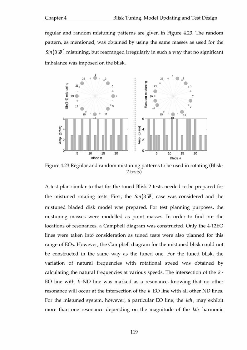
Chapter 4 Blisk Tuning, Model Updating and Test Design
119
regular and random mistuning patterns are given in Figure 4.23. The random
pattern, as mentioned, was obtained by using the same masses as used for the
( )8Sin θ⋅ mistuning, but rearranged irregularly in such a way that no significant
imbalance was imposed on the blisk.
21
19
17
1513
11
9
7
5
23 3 1
5 10 15 200
2
4
6
Blade #
Am
p. (
gram
)
5 10 15 200
2
4
6
Blade #
Am
p. (
gram
)
21
19
17
1513
11
9
7
5
23 3 1
Sin
(8 θ
) m
istu
ning
Ran
dom
mis
tuni
ng
Figure 4.23 Regular and random mistuning patterns to be used in rotating (Blisk-2 tests)
A test plan similar to that for the tuned Blisk-2 tests needed to be prepared for
the mistuned rotating tests. First, the ( )8Sin θ⋅ case was considered and the
mistuned bladed disk model was prepared. For test planning purposes, the
mistuning masses were modelled as point masses. In order to find out the
locations of resonances, a Campbell diagram was constructed. Only the 4-12EO
lines were taken into consideration as tuned tests were also planned for this
range of EOs. However, the Campbell diagram for the mistuned blisk could not
be constructed in the same way as the tuned one. For the tuned blisk, the
variation of natural frequencies with rotational speed was obtained by
calculating the natural frequencies at various speeds. The intersection of the k -
EO line with k -ND line was marked as a resonance, knowing that no other
resonance will occur at the intersection of the k EO line with all other ND lines.
For the mistuned system, however, a particular EO line, the kth , may exhibit
more than one resonance depending on the magnitude of the kth harmonic
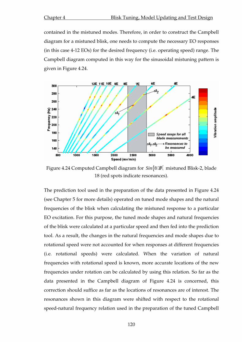
Chapter 4 Blisk Tuning, Model Updating and Test Design
120
contained in the mistuned modes. Therefore, in order to construct the Campbell
diagram for a mistuned blisk, one needs to compute the necessary EO responses
(in this case 4-12 EOs) for the desired frequency (i.e. operating speed) range. The
Campbell diagram computed in this way for the sinusoidal mistuning pattern is
given in Figure 4.24.
Figure 4.24 Computed Campbell diagram for ( )8Sin θ⋅ mistuned Blisk-2, blade
18 (red spots indicate resonances).
The prediction tool used in the preparation of the data presented in Figure 4.24
(see Chapter 5 for more details) operated on tuned mode shapes and the natural
frequencies of the blisk when calculating the mistuned response to a particular
EO excitation. For this purpose, the tuned mode shapes and natural frequencies
of the blisk were calculated at a particular speed and then fed into the prediction
tool. As a result, the changes in the natural frequencies and mode shapes due to
rotational speed were not accounted for when responses at different frequencies
(i.e. rotational speeds) were calculated. When the variation of natural
frequencies with rotational speed is known, more accurate locations of the new
frequencies under rotation can be calculated by using this relation. So far as the
data presented in the Campbell diagram of Figure 4.24 is concerned, this
correction should suffice as far as the locations of resonances are of interest. The
resonances shown in this diagram were shifted with respect to the rotational
speed-natural frequency relation used in the preparation of the tuned Campbell

Chapter 4 Blisk Tuning, Model Updating and Test Design
121
diagram. However, when response data are to be compared, the changes in the
mode shapes should also be considered. A way of doing this is presented in the
next chapter where the experimental and computed results are correlated.
As expected the Campbell diagram of Figure 4.24 was completely different to
that of the tuned blisk Figure 4.21. In particular, an interesting formation of two
distinct groups of resonances was evident where a persistent resonance at
around 280 Hz seemed to be excited by all EOs. To help explain this behaviour,
the mode shapes of the 1F family of modes needed to be calculated and
analysed. Accordingly, a full blisk model, complete with applied sinusoidal
mistuning pattern, was prepared and the first 24 modes (1F family) were
calculated. To make this model compatible with the measurements, the mode
shapes extracted from the FE analysis were represented by 24 points, each
corresponding to a blade tip location. Fourier analysis was performed on each
mistuned mode shape to determine the strong harmonics contained. A chart,
mapping the 4-12 spatial harmonics of the mode shapes of the 1F family of
modes is given in Figure 4.25.
12
11
10
9
8
7
6
5
4
271.
41
271.
13
271.
13
270.
65
270.
65
270.
45
270.
45
270.
41
248.
56
247.
47
247.
47
244.
14
244.
14
238.
11
238.
1
231.
56
214.
5
196.
04
196.
04
159.
51
159.
51
149.
92
145.
97
145.
97
Har
mon
ics
1F Natural frequencies (Hz)
Figure 4.25 Normalised amplitude spectrum of the first 12 spatial harmonics for
the first 24 Blisk 2 modes, with applied ( )8Sin θ⋅ mistuning.

Chapter 4 Blisk Tuning, Model Updating and Test Design
122
The harmonics map shown in Figure 4.25 correlates excellently with the
Campbell diagram of Figure 4.24, where darker colours indicate stronger
harmonics. For example, it is seen that three groups of modes at reasonably well
separated frequencies have significant 5 nodal diameter components, and would
therefore be strongly excited by 5EO. In fact, this is reflected in the Campbell
diagram as three resonances appearing on the 5EO line. The primary harmonics
contained in the first 16 modes were in ascending order. For modes 17 and
higher, this order was reversed with a primarily 8D mode being the highest in
frequency thus providing the expected modal overlap. Another interesting
revelation from the harmonics map was that it clearly indicated the number of
modes participating in a given resonance shown in Figure 4.24, which could not
be inferred from the response curves.
The FE analysis showed that there was not one but eight modes at around 270
Hz. Different engine orders excited different modes from this group, depending
on their harmonic content, but their frequencies were too close to be
differentiated visually in the Campbell diagram. Although many resonances
appeared in Figure 4.24, each was accounted for thanks to Fourier analysis.
Now that the resonance map of the regularly mistuned assembly was
constructed, a dynamic test plan similar for that of the tuned assembly could be
organized. The first step, likewise, was to measure the response on a particular
blade (i.e. the corresponding blade to that was used in the construction of the
computed Campbell diagram) for the full speed range so that a z-mod plot could
be obtained. An optimised speed vector was prepared according to the
identified locations of the resonances, similar to the one depicted in Figure 4.21,
only with more speed points due to scattered resonances.
As all the blades were now experiencing different vibration amplitudes, due to
the deliberate mistuning, measuring only one blade for a particular EO
excitation was not enough to account for blade-to-blade response variation.
Chapter 4 Blisk Tuning, Model Updating and Test Design
123
Therefore, all blades needed to be measured. If the same test plan which was
adopted for the tuned assembly was to be followed here (i.e. measuring 4-12EO
excitation responses but now for 24 blades), it would not be practical in terms of
the measurement times. Besides, most of the data would not add any extra
information so far as the validation of the prediction tool was concerned. Thus, it
was decided to concentrate on a specific EO excitation response and to explore
this in depth. To this end, the 6EO excitation response was chosen for study.
Equally, any of the 5-12 EOs could also have been selected. One particular
reason for going for the lower end of the EO range was to perform the tests
under relatively high rotational speeds. To this end, the 5EO excitation would
clearly be a better choice, but the modes it excited had mainly 5ND components
and were more affected by boundary conditions than the modes excited by 6EO
excitation. Only a limited speed range, covering the higher two resonances (the
third resonance was exciting a mainly 2ND mode and the disc fixing would have
a significant effect on it, which was not accounted for in the predictions)
appearing on the 6EO line was chosen to be swept, as shown by the grey band in
Figure 4.24.
The test plan for the random mistuning pattern case was very similar to that of
the case of regular mistuning. An interference diagram covering 4-12 EO lines
was prepared using the FE model of Blisk-2 with applied random mistuning.
This diagram is given in Figure 4.26. It must be noted that, unlike the sinusoidal
mistuning case, in the randomly mistuned blisk, considerably different
interference diagrams were obtained (depending on which blade’s response is
used). In selection of measurement speed ranges, the responses of all blades
were taken into consideration. Here only the diagram constructed for blade 20
(selected arbitrarily) is given for brevity.

Chapter 4 Blisk Tuning, Model Updating and Test Design
124
Figure 4.26 Computed Campbell diagram for random mistuned Blisk-2, blade 20
The resonances shown on the diagram, Figure 4.27, are accounted for by the
harmonics map of the 1F family of modes, prepared using the same full FE
model as used for regular pattern but here with random mistuning applied.
Since the random nature of the mistuning caused modes to be more irregular,
more resonances were excited by a given EO excitation. Again, a speed vector
encompassing the entire range, based on the interference diagram, was
constructed for z-mod plot measurements.
12
11
10
9
8
7
6
5
4
274.
39
272.
83
271.
35
270.
95
270.
85
268.
39
268.
28
266.
72
255.
89
253.
26
252.
83
244.
51
240.
2
237.
12
231.
91
224.
73
218.
49
198.
21
195.
79
160.
62
159.
63
149.
72
147.
03
144.
75
Har
mon
ics
1F Natural frequencies (Hz)
Figure 4.27 Normalised amplitude spectrum of the first 12 spatial harmonics for the first 24 Blisk 2 modes, with applied random mistuning.

Chapter 4 Blisk Tuning, Model Updating and Test Design
125
All blade measurements in the random mistuning case were chosen for the
range shown in grey in Figure 4.26. The choice of 10EO (an EO on the higher end
of 4-12EO range) was made because of the high resonance density it provided in
a relatively short speed range (there are 5 resonances in this region, only 3 of
them strongly excited for the given blade). The predictions for this high density
region would therefore set a challenging task for the prediction tool. Equally,
other EOs (8, 9, 11 or 12) could also be selected.
4.4.2 Undamped and damped tests on Blisk-1
The planning of the friction damping tests on Blisk-1 with integral dampers
followed more or less the same guidelines but was a more challenging task,
particularly due to uncertainties brought in with the non-linear nature of the
under-platform friction dampers. Moreover, the lack of a tuned reference state of
the blisk (though this has been compensated to a degree through model
updating and mistuning identification techniques) also complicated the test
planning.
The main objective of the friction damped Blisk-1 tests was to validate the
predictions of a numerical code through which the forced response of an entire
bladed disk can be calculated in the presence of various types of non-linearities,
including under-platform friction dampers. More details on the prediction tool
can be found in Chapter 6. However, it was though appropriate to measure the
corresponding undamped configurations as well, so that: (i) the errors
introduced via the FE model could be inferred and, if possible, corrected
through less complicated and less uncertain linear forced response
computations, thereby limiting the source of uncertainties in the computations to
non-linear elements, and (to a lesser extent) (ii) the effectiveness of the dampers
could be assessed by comparing damped and undamped responses.
Chapter 4 Blisk Tuning, Model Updating and Test Design
126
For a linear structure, once a convincing FE model is obtained, it is possible to
come up with a reasonably accurate test plan which can be closely followed in
practice, even if some minor modifications are often inevitable during
implementation. However, with non-linear systems this cannot be taken for
granted as modelling of the actual behaviour of the non-linear components is
somewhat less certain and the results will vary depending on the modelling of
the non-linearity. Besides, even if the model is sufficiently accurate, reliable
estimates of the values of non-linear parameters such as friction coefficient and
contact stiffness are often not available during the planning phase. Therefore it is
important that the test planning is made as flexible as possible so that a range of
options can be covered.
One of the most important things in the planning of tests with friction dampers
is to determine the speed range in which the dampers will operate successfully.
Since a damper always has a finite mass, the centrifugal load exerted on it
increases with increasing speed and at a certain point becomes too high, thereby
preventing it from functioning properly. Dampers in such a state are said to be
locked-up. In this situation, the neighbouring blades are interconnected through
dampers which lead to substantial stiffness increases in the assembly, thus
resulting in the natural frequencies being raised. Often the shifts in natural
frequencies are considerably higher so that exciting the “new” resonances may
not be possible within the speed range of the test setup.
In order to reduce the possibility of such a situation, it is essential that certain
parameters such as damper mass, excitation forces, operating speed range etc.
are determined accordingly. It was decided to use so-called “Cottage-Roof” (CR)
dampers in the experiments since they were commonly used in real engines and
relatively cheap to manufacture. A rather simple methodology was adopted to
calculate a rough estimate for the damper mass. The dampers were considered
in their stuck position (i.e. no relative motion between the dampers and blades),
so that the system behaved linearly. The idea was to work out the relationship
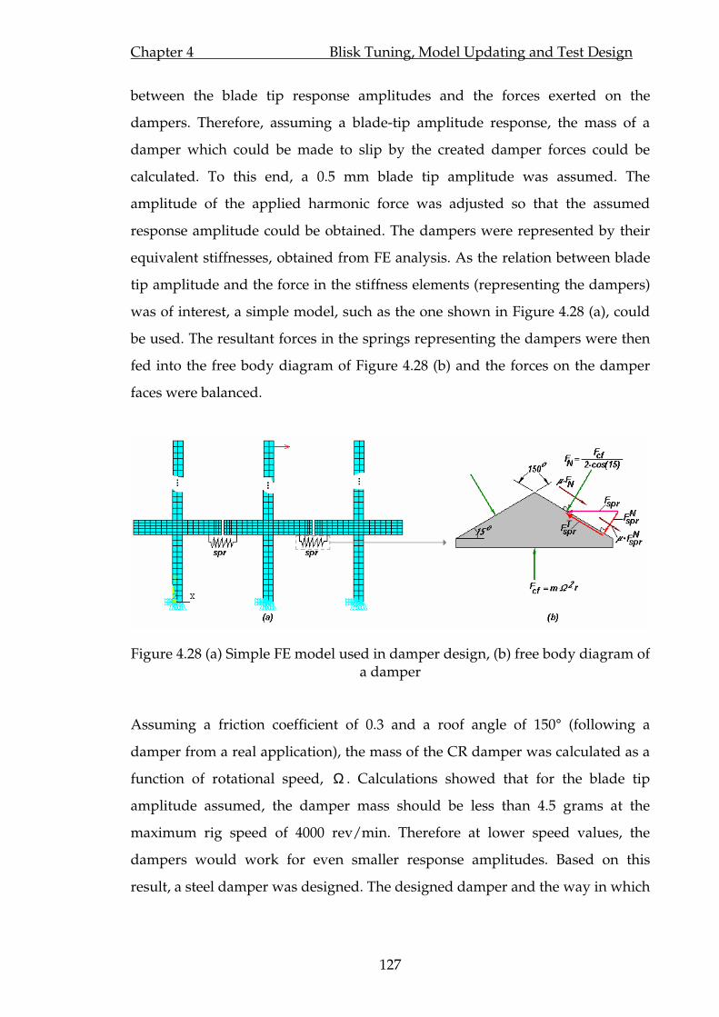
Chapter 4 Blisk Tuning, Model Updating and Test Design
127
between the blade tip response amplitudes and the forces exerted on the
dampers. Therefore, assuming a blade-tip amplitude response, the mass of a
damper which could be made to slip by the created damper forces could be
calculated. To this end, a 0.5 mm blade tip amplitude was assumed. The
amplitude of the applied harmonic force was adjusted so that the assumed
response amplitude could be obtained. The dampers were represented by their
equivalent stiffnesses, obtained from FE analysis. As the relation between blade
tip amplitude and the force in the stiffness elements (representing the dampers)
was of interest, a simple model, such as the one shown in Figure 4.28 (a), could
be used. The resultant forces in the springs representing the dampers were then
fed into the free body diagram of Figure 4.28 (b) and the forces on the damper
faces were balanced.
Figure 4.28 (a) Simple FE model used in damper design, (b) free body diagram of a damper
Assuming a friction coefficient of 0.3 and a roof angle of 150° (following a
damper from a real application), the mass of the CR damper was calculated as a
function of rotational speed, Ω . Calculations showed that for the blade tip
amplitude assumed, the damper mass should be less than 4.5 grams at the
maximum rig speed of 4000 rev/min. Therefore at lower speed values, the
dampers would work for even smaller response amplitudes. Based on this
result, a steel damper was designed. The designed damper and the way in which

Chapter 4 Blisk Tuning, Model Updating and Test Design
128
was integrated into the blisk are given in Figure 4.29. Assuming the density of
Steel to be 7800 kg/m3, the damper mass was found to be 4.2 gram.
Figure 4.29 Designed damper and its integration
The simplifying assumptions necessitated further measures to be taken to ensure
the success of the test campaign. For this purpose it was decided that another set
of dampers should be made from a lighter material in case the original ones
proved too heavy to be effective. The material for the second set of dampers was
chosen to be Titanium which reduced the damper mass to 2.2 grams. Another
measure taken was to make the necessary provision so that the excitation force
could be increased, should there be need for it, as documented in Chapter 3.
Following the same procedure as used for Blisk-2, first, an FE based interference
diagram was constructed for the 1F family of modes of undamped Blisk-1, and is
given in Figure 4.30 (necessary forced response calculations were carried out
using the prediction tool to be validated. More details on the code are given in
Chapter 5 and the way in which the identified mistuning is presented to the
code is given in Chapter 6). Based on this diagram, a variable-step speed vector
was prepared to measure a single blade for z-mod plots. Both blisks possessed
similar damping characteristics, therefore the same number of measurement
points as taken around Blisk-2 resonances was chosen for Blisk-1 as well. In
order not to complicate the computations further by mistuning, it was
considered favourable to measure the response at resonances corresponding to

Chapter 4 Blisk Tuning, Model Updating and Test Design
129
the lower ND modes as they were known to be sufficiently tuned. However, as
lower ND modes were excited at high rig speeds, there was a risk of dampers
locking up due to high centrifugal forces. Eventually, it was decided to make
arrangements for three speed bands to cover the damped and undamped
characteristics of Blisk-1.
Figure 4.30 Computed Campbell diagram for updated Blisk-1 FE model including inherent mistuning, 4-24 EOs
The first band concentrated around the 5EO-5ND resonance covering a range
shown by the light grey band on the computed interference diagram given in
Figure 4.30. The 5ND mode was so reasonably tuned that uncertainties in
mistuning identified or in its modelling would not have an adverse effect on the
predictions. The second band of measurements, shown by a darker grey colour,
was intended for undamped tests. A closer inspection of the computed 9EO
response curve revealed the occurrence of a number of resonances (note that
primarily 9D modes were significantly mistuned even after the tuning process).
By then the ability of the numerical code to predict the mistuned response
accurately will have been demonstrated via Blisk-2 measurements. Therefore,
the measurements around this resonance should provide the necessary data to
assess the degree to which the mistuning has been correctly identified or
modelled. The third speed band shown in dark green was envisaged as being
used in the event of the dampers not working in the first band. It covered the

Chapter 4 Blisk Tuning, Model Updating and Test Design
130
resonances corresponding to the 4-7 ND modes but this time excited by 20-17
EOs, respectively (i.e. for a bladed disk having 24 blades an n ND mode will be
excited by n , 24 n− , 24 n+ etc EOs due to spatial aliasing). Therefore, the first 24
EO excitation responses, as shown in Figure 4.30, needed to be calculated. Since
these resonances were excited at relatively low rotational speeds, the chances of
the dampers working properly are higher. Also, they corresponded to
reasonably tuned ND modes which would reduce the uncertainties in
computations. The third band covered a range of resonances. However, the
actual measurements were to be conducted for a range covering one or two of
them because of testing time considerations.
Ideally, it would be desirable to construct an interference diagram (similar to the
one computed for the undamped case) for the blisk with integrated CR dampers.
However, doing this would be computationally very expensive, especially
bearing in mind that it would have to be repeated several times to improve the
design. Moreover, at the time the test design was undertaken, the prediction tool
was not yet coded to handle such big assemblies.
4.5 Summary
In this chapter three issues have been addressed: (i) identification of the
reference tuned states of the blisks, (ii) updating of their FE models, and (iii) the
design of tests in the run up of the real tests and the validation of the
predictions, have been addressed.
Through FRF and ODS measurements at rest, Blisk-2 has demonstrated that it
can act as a suitable tuned reference for forced response calculations. Blisk-1, on
the other hand, has been found to be significantly mistuned. Although a tuning
process has been undertaken to improve the tuned state of Blisk-1 (and to a
certain degree this has been achieved) it has not been possible to establish a
sufficiently reasonable tuned state to provide a suitable reference case. Blisk

Chapter 4 Blisk Tuning, Model Updating and Test Design
131
tuning has been studied via a lumped parameter blisk model to see if better
accuracy could have been obtained had the tuning been performed in different
ways. The results have showed that, by matching 1F blade-alone frequencies, the
symmetry of the blisk can be improved to a certain extent, but only if
modifications are introduced through appropriate parameters. However, it has
been concluded that, ultimately, more than one frequency of the blade-alone
models will have to be matched, using appropriate parameters, for higher
accuracy. These parameters should be identified based on their influence on the
assembly properties.
The FE models of the blisks have been updated based on the mode shapes and
the natural frequencies measured on the real bladed disks that they are expected
to represent. The IES updating method has been used for the FE model of Blisk-2
and a combination of the IES and FMM-ID methods have been used to update
the FE model of Blisk-1. The results obtained by employing these models have
been demonstrated to correlate closely with measurements. The difference
between measured and FE natural frequencies, resulting mainly from
dimensional variations in the blisk, has been reduced by using the material
properties as updating parameters. As a result, somewhat unrealistic material
properties, density in particular, have resulted from the updating process.
Finally, based on the updated FE models of the blisks, a comprehensive test plan
has been prepared in an attempt to make the actual testing more efficient. Tuned
and mistuned tests with Blisk-2 have been planned. The mistuning shapes and
strengths to be applied have been chosen and the resonances to be measured
identified. Undamped and damped Blisk-1 tests have also been designed. The
damped testpiece test plan, compared with the undamped one, is less reliable
due to the uncertainties associated with the friction dampers and may need to be
modified during the execution of tests.
Chapter 5 Validation of Tuned and Mistuned Blade Response Predictions
132
CHAPTER 5
VALIDATION of TUNED and
MISTUNED BLADE RESPONSE
PREDICTIONS
5.1 Overview
Having prepared the necessary ingredients in the previous chapters, it is now
time to compare forced response predictions for the tuned and mistuned Blisk-2
with the measurements taken under rotation. To this end, the numerical code to
be used in calculations, and therefore the one sought to be validated, is first
introduced. Then, starting with the stationary/mistuned tests, following the test
plan drawn in the previous chapter, the results obtained from rotating/tuned,
and sinusoidally- and randomly-mistuned Blisk-2 are presented. The predictions
are correlated with these results and the degree of success and the possible
sources of discrepancies are discussed.
5.2 The prediction tool
The existing mistuned bladed disk response prediction tool sought to be
validated here exploits an exact relation between the tuned and mistuned
assemblies’ dynamic properties. The complete derivation of the method is given
in [14]: there the main features and the use of the method are summarised.
The main goals of the method for calculation of mistuned forced response are
achieved: (i) without inverting a matrix, (ii) by using a cyclic sector (as in the
case of tuned calculations), and (iii) by including the contribution of all the

Chapter 5 Validation of Tuned and Mistuned Blade Response Predictions
133
degrees-of-freedom, thus avoiding the errors which can occur in conventional
reduction processes.
The application of the method can be summarised as follows: first, the tuned
assembly’s mode shapes and natural frequencies are calculated for a number of
families of modes of interest, using a cyclically symmetric sector FE model. Then
the DOFs where the mistuning is to be introduced and response levels are to be
calculated are identified. Together with the DOFs where the excitation forces are
applied, these coordinates are called “active DOFs” and all the remaining ones
are “passive DOFs”. They are named in this way because the active DOFs are
involved explicitly in the calculations of both tuned and mistuned assemblies,
whereas the passive ones are not, being used only in tuned response
calculations. A subset of tuned assembly mode shapes is prepared by extracting
the values at the identified active DOFs, together with the tuned natural
frequencies and applied mistuning, and used in the mistuned computations.
With such partitioning, the matricies involved in the mistuned response
calculations are reduced to much smaller sizes without loss of accuracy. This
provides the ability to calculate the forced response, at the DOFs of interest in
much reduced computation times.
Physical mistuning is introduced via so-called “mistuning elements” at desired
nodes of the sector FE model. These relatively simple but efficient mistuning
elements include: lumped mass, discrete stiffness and damping elements applied
between a node and the ground, or between two nodes. Values of the mistuning
applied in each coordinate direction at a given node can be different. Although
many mistuning patterns can be defined by mistuning elements, mistuning is
often expressed in terms of the variation of blade-alone natural frequency or
frequencies (i.e. those of a separate or isolated blade). This kind of mistuning is
accommodated in the method by establishing a relationship between the known
frequency scatter and the properties of a set of mistuning elements defined at
certain nodes. In this way, the given frequency mistuning is translated to

Chapter 5 Validation of Tuned and Mistuned Blade Response Predictions
134
physical mistuning, through these mistuning elements, such that the blades with
applied mistuning elements exhibit a specified frequency variation.
The method is coded into a computer program, MISTuning RESponse
(MISTRES), to perform forced response calculations for a desired EO excitation.
The type of excitation and mistuning, response DOFs, frequency range of
interest, etc are provided through a general input file. Additionally, another file
containing the mode shape data corresponding to DOFs of interest for the
included modes of the tuned assembly, and natural frequencies of these modes,
is submitted. If the mistuning is defined in terms of natural frequency variation
of sub-models (e.g. of isolated blades), then another file, similar to the second
one, for each sub-model is also provided. The outputs of the code are: (i)
response levels at the desired nodes of the FE model (which can be calculated for
all available DOFs separately, or as a total response at those nodes); (ii)
maximum responding blade for all the resonances, and (iii) natural frequencies,
within the frequency range of analysis. Blade-to-blade amplitude variations at
the frequencies corresponding to excited resonances are also output.
5.3. Mistuning analysis on the stationary blisk
In accordance with the test plan prepared in Chapter 4, a number of mistuning
patterns were selected and applied to Blisk-2 and the natural frequencies and the
mode shapes measured, non-rotating, before the dynamic tests were started. By
doing this it would be possible to gauge the ability of the prediction tool to
predict the correct natural frequencies and vibration amplitude variations when
excited at these frequencies in the absence of rotation. Three mistuning patterns
were considered: (i) Single blade mistuning (SBM), (ii) sinusoidal mistuning
( ( )12Sin θ⋅ ), and (iii) random mistuning. The applied mistuning patterns are
illustrated in Figure 5.1.

Chapter 5 Validation of Tuned and Mistuned Blade Response Predictions
135
2 4 6 8 10 12 14 16 18 20 22 240
0.5
1
1.5
2
2.5
3
Am
plitu
de (g
ram
)
2 4 6 8 10 12 14 16 18 20 22 240
0.5
1
1.5
2
Blade #2 4 6 8 10 12 14 16 18 20 22 24
0
0.5
1
1.5
2
2.5
3
SBM Sin(12 θθθθ) Random
Figure 5.1 Mistuning patterns applied to stationary Blisk-2.
Mistuning of Blisk-2 was achieved by attaching washers via small bolts to the
blade tips. Updating of the FE model of Blisk-2 was covered in the previous
chapter, where it was demonstrated that it simulated the characteristics of the
real blisk satisfactorily. Therefore, it is fair to assume that the degree of
correlation of these tests with predictions will depend on the modelling of the
applied mistuning. In the FE model, mistuning weights were modelled as point
masses, applied in the middle of the blade tip outer surfaces but distributed over
a number of nodes. This was reasonable as the centres of mass of these masses
laid very close to the mentioned surfaces. The resultant frequency splits
(separation of double modes) in 1F family double modes (i.e. 1-11ND) of Blisk-2
are given in Figure 5.2.
1 2 3 4 5 6 7 8 9 10 110
0.5
1
1.5
2
2.5
Fre
quen
cy S
pilt
(Hz)
1 2 3 4 5 6 7 8 9 10 110
2
4
6
8
10
12
14
Dominant ND
Exp.MISTRES
1 2 3 4 5 6 7 8 9 10 110
0.5
1
1.5
2
2.5
3
SBM Sin(12 θθθθ) Random
Figure 5.2 Split in 1F family double modes due to applied mistuning patterns
Experimental results corresponding to some of the mode pairs are missing from
SBM and random cases given above. This is not necessarily because these modes

Chapter 5 Validation of Tuned and Mistuned Blade Response Predictions
136
do not split, but some of the frequencies, despite several attempts, could not be
captured in the experiments. In principle, a mistuning pattern will split an n ND
mode only if a 2n harmonic is present in its Fourier series representation.
Therefore, the SBM mistuning pattern is expected to cause all, and the given
random mistuning pattern should cause all but 6ND, modes to split. Similarly
only the 6ND mode is expected to be split in case of ( )12Sin θ⋅ mistuning
pattern. The predicted results were supported gratifyingly closely by the
available measured counterparts, both in terms of split patterns and amplitudes.
Individual natural frequency values were predicted with errors less than 0.2%.
Nevertheless, some deviations were evident, probably due to errors in
mistuning and boundary condition modelling in the FE model.
ODSs corresponding to the “random” case were measured for the 1F family of
modes so that they could be compared with the predicted ones. The choice of
random case was particularly challenging for the FE prediction model because of
the complexity and variability produced in the mode shapes. Circumferential
ODS measurements were performed using an SLDV and an electromagnet, as
explained in Chapter 3.5. Some of the measured ODSs encompassing natural
frequencies from the lower and higher ends of 1F family of modes are compared
with the predicted ones in Figure 5.3. Since the modes are distorted by applied
mistuning, they are numbered from 1 to 24 rather than using the ND notation
which does not apply to all of them. The numerical code used, MISTRES, is
intended for the calculation of the forced response amplitudes. As a result, the
outputs are not “signed”. For clarity of the comparisons, therefore, absolute
values as well as signed ODSs of the experiments are given in the presented
plots. The measured ODSs were obtained by scanning the blisk continuously at
platform level. However, each blade is represented in predictions by a single
point in the middle of the blade at platform level. This is appropriate as the out-
of-plane flexural modes are of interest. Very good agreement is obtained, not
only for regular lower natural frequency modes but also for highly localised
higher ones. During the measurements , the electromagnetic force input was not

Chapter 5 Validation of Tuned and Mistuned Blade Response Predictions
137
measured since it required an additional and complicated fixture. The
predictions have therefore been normalised by the amplitude of the maximum
responding blade in the measurements.
0 180 360-1.5
-1
-0.5
0
0.5
1
1.5
Nor
mal
ised
am
plitu
de
0 180 360-2
0
2
4
0 180 360
-2
-1
0
1
2
Angular position (degree)0 180 360
-2
-1
0
1
2
3 Exp.|Exp|MISTRES
Mode # 7
Mode # 17
Mode # 15
Mode # 24
Figure 5.3 Comparison of ODSs for stationary Blisk-2 with applied random mistuning.
5.4 Tuned and mistuned analysis on rotating blisk
In a validation study, it is important that one step is taken at a time so that the
contribution of every new feature can be properly interpreted and accounted for.
Following this, the rotating tests were conducted in three steps. First, the tuned
blisk was tested, to provide a reference set of data, and necessary inputs, such as
damping and force magnitudes, for numerical predictions. Then, measurements
on regularly and randomly mistuned blisk configurations were executed,
according to the agreed test plan.
5.4.1 Repeatability of rotating measurements
Before the rotating tests could begin in earnest, the ability of the rig to reproduce
the same data under the same/similar conditions at different times had to be
checked. This would provide confidence in the data supplied by the rig,

Chapter 5 Validation of Tuned and Mistuned Blade Response Predictions
138
establishing it as a “well-controlled” environment for precise vibration
measurements.
To this end, the technique devised (Chapter 4.2.2) was thought appropriate to
check the tuned state of Blisk-2 under stationary conditions. Following the same
procedure, a selected mistuning pattern was applied to the blisk and a particular
blade’s response was measured for a specific speed range. Then the mistune
pattern was shifted by a number of blades around the blisk, as shown in Figure
5.4 (a), and the “same” blade was re-measured for the same range. This test,
therefore, would not only assess the repeatability of the measurements but
would also gauge the effect of any asymmetry (i.e. inherent mistuning) in the
blisk, if present, on forced response under rotation. The results obtained for the
original and shifted patterns are given in Figure 5.4 (b).
1200 1300 1400 1500 1600 1700-40
-30
-20
-10
0
10
20
Rotor speed (rev/min)
Am
plitu
de (
dB)-
re
100
mm
/s
Pattern 1Pattern 2
(a)
(b)
Pat
tern
2
P
atte
rn
1
Figure 5.4 (a) Original and shifted mistuning patterns, (b) comparison of 10-EO response curves for both patterns – shaded circles indicate corresponding
measurement locations.
The applied mistuning pattern was the one chosen to be used in random
mistuning analyses on Blisk-2. Given the complexity of the test rig and the
measurement system, the excellent agreement between curves in Figure 5.4

Chapter 5 Validation of Tuned and Mistuned Blade Response Predictions
139
constitutes good evidence of the repeatability of the tests and also the suitability
of the blisk as a tuned reference under rotation.
5.4.2. Inclusion of rotation in forced response predictions
The frequency of excitation in measurements varied with rotational speed, thus
the natural frequencies and to an extent the mode shapes of the blisk, changed as
the speed changed, due to centrifugal stiffening. MISTRES uses the mode shapes
and natural frequencies of the tuned system, and once these inputs are provided
they remain the same for all frequencies of that forced response calculation
session. Therefore, in order to simulate the actual behaviour in the rig precisely,
one has to calculate the response at each speed point by using mode shapes and
natural frequencies calculated at that particular speed. However, this is
extremely time consuming and is not entirely necessary. In terms of natural
frequencies, a near exact relationship can be obtained between rotational speed
and the frequency shift by calculating frequencies at a few speed values and
then fitting a quadratic curve to these values (the change in natural frequencies
of the 1F family of modes is proportional to the square of the rotational speed).
Therefore, once the forced response calculations for a given set of modal data are
complete, the frequency axis can be modified to reflect the effects of rotational
speed. As for the mode shapes, and particularly when response is to be
calculated in a limited frequency (i.e. rotation speed) range (e.g. a range of 100-
300 rev/min), mode shape and natural frequency data calculated at mid-speed
range value provide sufficiently accurate results. This is because the mode
shapes do not change much with rotation, over such small ranges. An example
of this is given in Figure 5.5 where the 6EO response is calculated using mode
shapes calculated at both 2500 rev/min and also at a speed corresponding to 1F
6EO-6ND resonance, 2756 rev/min. The green curve represents the results
obtained for the former case, before frequency shift. For the blue and red curves,
the frequency axes are arranged to reflect the effect of rotation (i.e. in case of the
blue curve, all the frequencies corresponding to values higher than 2500

Chapter 5 Validation of Tuned and Mistuned Blade Response Predictions
140
rev/min are shifted to the right in accordance with the speed-frequency shift
relation). Resonance frequencies of the red and blue curves were practically the
same; response amplitudes showed differences of up to 0.05%. Bearing in mind
that the speed ranges of interest are smaller than that of this particular case, thus
resulting in smaller deviations, the handling of the effects of rotation in this way
is entirely justifiable.
250 255 260 265 270 275 280 285 290 295 300-60
-50
-40
-30
-20
-10
0
10
20
ω, Freqeuncy (Hz)
Am
plitu
de (
dB)
[φ, ωn] @ 2500 rev/min[φ, ωn] @ 2500 rev/min - ω shifted[φ, ωn] @ 2756 rev/min - ω shifted
Blue curve, +ω shift
Ω = 2500 rev/min
Ω = 2756 rev/min +ω shift -ω shift
red curve
Figure 5.5 Comparison of 6EO excitation response using mode shapes calculated at different speeds.
5.4.3 Evaluation of forcing input
Excitation was achieved through a permanent magnet fixed in space. In their
normal operation the bladed disks with this arrangement are being excited by
phased pulses generated by the magnet each time a blade rotates past. The
excitation force fluctuates from near-zero when the magnet is between blades, to
a maximum when the magnet is centred on a blade tip. Note that this type of
forcing is different and more realistic than applying harmonically pure phased
pulses to a static blisk [55, 49] (i.e., )( θω ⋅+⋅⋅= itSinAFi , where A is the
amplitude, ω is excitation frequency t is time, θ is inter-blade angle and i is
the blade number). In the present case, the magnet only attracts the blades;
therefore, all the force values are positive. Hence the forcing consists of,
predominantly, a mean level at zero frequency, and a harmonic at the

Chapter 5 Validation of Tuned and Mistuned Blade Response Predictions
141
fundamental forcing frequency (rotational speed X # of blades) as well as some
lower amplitude harmonics that appear at integer multiples of the fundamental
forcing frequency. A train of typical magnet pulses generated during the
operation of the rig with Blisk-2 is given in Figure 5.6. Also shown in this figure
is the magnet force applied to a particular blade in one rotation cycle of the blisk
(note that only a portion of rotation cycle is given here).
Figure 5.6 A typical train of magnet pulses applied to Blisk-2 @ 120 rev/min.
Given a magnet pulse such as the one given in red in Figure 5.6, the amplitudes
of the force exciting different EOs can be calculated by performing a Fourier
series analysis. Assuming that the discrete force signal, f , is defined at N time
points, ktt = ( Nk ,...,2,1= ) and is periodic, with a period T , in the form
)()( Ttftf += , it can be represented by a finite series:
−
==
1
0
/2N
n
Ninknk eXf π
(5.1)
where
NnefN
XN
k
Ninkkn ,...,2,1,
1 1
0
/2 == −
=
− π. (5.2)
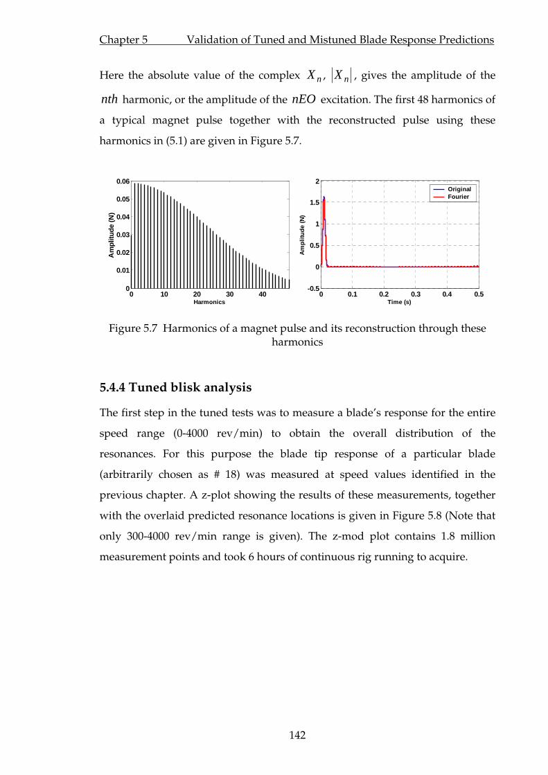
Chapter 5 Validation of Tuned and Mistuned Blade Response Predictions
142
Here the absolute value of the complex nX , nX , gives the amplitude of the
nth harmonic, or the amplitude of the nEO excitation. The first 48 harmonics of
a typical magnet pulse together with the reconstructed pulse using these
harmonics in (5.1) are given in Figure 5.7.
0 10 20 30 400
0.01
0.02
0.03
0.04
0.05
0.06
Harmonics
Am
plitu
de (N
)
0 0.1 0.2 0.3 0.4 0.5-0.5
0
0.5
1
1.5
2
Time (s)A
mpl
itude
(N)
OriginalFourier
Figure 5.7 Harmonics of a magnet pulse and its reconstruction through these harmonics
5.4.4 Tuned blisk analysis
The first step in the tuned tests was to measure a blade’s response for the entire
speed range (0-4000 rev/min) to obtain the overall distribution of the
resonances. For this purpose the blade tip response of a particular blade
(arbitrarily chosen as # 18) was measured at speed values identified in the
previous chapter. A z-plot showing the results of these measurements, together
with the overlaid predicted resonance locations is given in Figure 5.8 (Note that
only 300-4000 rev/min range is given). The z-mod plot contains 1.8 million
measurement points and took 6 hours of continuous rig running to acquire.
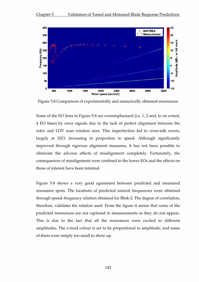
Chapter 5 Validation of Tuned and Mistuned Blade Response Predictions
143
Figure 5.8 Comparison of experimentally and numerically obtained resonances
Some of the EO lines in Figure 5.8 are overemphasised (i.e. 1, 2 and, to an extent,
4 EO lines) by error signals due to the lack of perfect alignment between the
rotor and LDV scan rotation axes. This imperfection led to cross-talk errors,
largely at 1EO, increasing in proportion to speed. Although significantly
improved through rigorous alignment measures, it has not been possible to
eliminate the adverse effects of misalignment completely. Fortunately, the
consequences of misalignment were confined to the lower EOs and the effects on
those of interest have been minimal.
Figure 5.8 shows a very good agreement between predicted and measured
resonance spots. The locations of predicted natural frequencies were obtained
through speed–frequency relation obtained for Blisk-2. The degree of correlation,
therefore, validates the relation used. From the figure it seems that some of the
predicted resonances are not captured in measurements as they do not appear.
This is due to the fact that all the resonances were excited to different
amplitudes. The z-mod colour is set to be proportional to amplitude, and some
of them were simply too small to show up.

Chapter 5 Validation of Tuned and Mistuned Blade Response Predictions
144
The comparison shown in Figure 5.8 does not provide enough resolution to
assess the degree of correlation precisely. In order to do this, individual EO
response curves needed to be measured, and with finer speed steps as planned
earlier. This was also necessary so that the actual force and damping values
could be measured and identified for absolute response levels. For this purpose
the response to 6EO was measured. Measured response amplitude and phase
plots are given in Figure 5.9 (a) and (b) respectively. As anticipated in the test
design phase, true resonance peak amplitudes could not be measured due to the
extremely light damping. Very high vibration amplitudes in the immediate
neighbourhood of the resonance frequency led the LDV transducer to overload
(despite using the minimum possible sensitivity), resulting in the notch seen on
Figure 5.9 (a). Inspection of the time signals (also shown in the figure) around
the resonance revealed that overloading occurred in the range between the
points marked as “1” and “3”, clearly seen from the time signal given for point
“2”. It was a limitation in the LDV transducer’s electronics that it truncated
signals larger than 20V p-p. Moreover, with large vibration amplitudes, the
measurement point shifted, sometimes, to such positions where speckle noise
became significant and disturbed the measured signal grossly, in the form of
drop-outs. As this signal was low-pass filtered in the LDV’s head, the time
signals measured by the DAQ board were much reduced in amplitude and
showed some higher harmonics as seen from the time signal corresponding to
point “2”. This fact should be taken into consideration in the analyses of
measured data and their comparison with predictions.

Chapter 5 Validation of Tuned and Mistuned Blade Response Predictions
145
2700 2720 2740 2760 2780 2800-25
-20
-15
-10
-5
0
5
10
15
Rotor speed (rev/min)
Am
plitu
de (
dB)
- re
100
mm
/s
2745 2750 2755 2760 2765
0
50
100
150
Rotor speed (rev/min)
Pha
se (
deg)
-4
-2
0
2
4
Time
Am
p (V
)
-5
0
5
Time
Am
p (V
)
-5
0
5
Time
Am
p (V
)
1
2
3
(a)
(b)
Maximum dampingenvelope
η=2*ωn /tan(α)
ωn
α
~
Figure 5.9 (a) Amplitude, and (b) phase plots of 6EO forced response on blade #1.
Frequency response data of Figure 5.9 were analysed in ICATS to find out the
damping value to be used in predictions. Discarding the points between “1” and
“3”, the structural damping loss factor, η , was found to be 0.005%. Unreliable
measurements around the resonance made damping identification somewhat
uncertain. However, it was possible to define a conservative upper bound for
damping value from the phase plot. Assuming an SDOF behaviour around this
resonance, the slope of the phase vs. normalised frequency ( / nω ω ) plot gives the
inverse of critical damping ratio, ζ . Therefore by considering the slope of the
red curve in Figure 5.9 (b), and using 2η ζ= at resonance, a conservative value
of the loss factor could be obtained. This calculation gave a loss factor of 0.01%.
This result, as an upper bound, was reasonable as the damping value measured
at rest and in the presence of air was 0.01%. Therefore, it was decided that a
damping value of 0.0075% (mean of 0.005 and 0.01) to be used in the predictions.
Measurements were taken from the mid blade tip area, and therefore FE
responses were extracted from the same location. Excitation force, measured in
the form of pulses, was decomposed into its harmonics using Fourier analysis as
described in the previous section. Predicted and measured responses to only 6, 8
and 12 EO excitations are given in Figure 5.10 for brevity. The magnet-blade gap
was different in each case, and, therefore the response amplitudes are similarly

Chapter 5 Validation of Tuned and Mistuned Blade Response Predictions
146
different. Natural frequencies and the mode shapes for these analyses were
calculated at 2756, 1965 and 1435 rev/min respectively. Frequency axes of the
given plots were rearranged as described previously.
270 272 274 276 278 280
-10
0
10
20
30
40
50
Frequency (Hz)
Am
plitu
de (d
B)
- re
100
mm
/s
276 278 280 282 284 286 288
-10
0
10
20
30
40
50
Frequency (Hz)280 282 284 286 288 290 292 294
-20
-10
0
10
20
30
40
50
Frequency (Hz)
MeasurementMISTRES
6EO 8EO 12EO
Figure 5.10 Comparison of response measurements for 6, 8 and 12 EO excitations (η =0.000075 in predictions).
Comparison given in Figure 5.10 presents a good match between measurements
and predictions. However, some deviations, particularly in terms of frequencies,
are evident. Although the variations in frequencies, in general, were around
0.2%, this was an increase compared to maximum stationary frequency
deviation of 0.1%. This might be explained by the change of boundary
conditions between stationary and rotating cases as well as changes in ambient
temperature. Although similar fixtures were used in both configurations,
unavoidably different setups had to be employed in rotating and stationary tests
(i.e. the static tests were carried out prior the manufacture of the rotating rig).
Also, due to the long time span of the testing process, the corresponding tests
had to be conducted at somewhat different ambient temperatures. At this level
of accuracy, differences of this magnitude due to these effects are not unusual.
The magnet-blade gap was reduced significantly to capture resonance
amplitudes more accurately, but to no avail. Therefore, to limit the blade
amplitudes the responses of all the blades were measured slightly off-resonance,
and compared with the predictions. For this purpose, the exact location of the

Chapter 5 Validation of Tuned and Mistuned Blade Response Predictions
147
resonance was located and the rotational speed increased by 1 rev/min to get
reduced amplitudes. With sufficiently large magnet-blade gaps, it has been
possible to obtain good signals at such speeds. The results of this comparison are
given in Figure 5.11. Predicted values at 1 rev/min away from the resonance are
considerably higher than the measured ones. Bearing in mind that the true
resonance frequency might not have been captured precisely during testing,
predicted values at 1.5 and 2 rev/min away from the resonance are also given.
Very close results are obtained for 1.5 rev/min case. It must be also noted that
the previously identified damping value might also be lower than during this
test, contributing to discrepancy between measured and predicted amplitudes.
5 10 15 200
2
4
6
8
10
12
14
Blade #
Am
plitu
de (d
B) -
re
100
mm
/s
Predicted @ 1 rev/min away from resonancePredicted @ 1.5 rev/min " "Predcited @ 2 rev/min " "Measured @ 1 rev/min away from identified resonance
2 4 6 8 10 12 14 16 18 20 22 24-200
-150
-100
-50
0
50
100
150
Blade #
Inte
r-bl
ade
phas
e an
gel (
deg)
Measured
Figure 5.11 Comparison of 6EO response amplitudes away from 6EO-6ND resonance and measured inter-blade phase angles.
Inter-blade phase angles plotted in Figure 5.11 suggest a pure travelling wave in
the blisk with constant 90° phase angles between the two adjacent blades. This
implies that all the blades experience the same vibration amplitude. Even though
a small ripple is apparent, this is backed by the even distribution given in the
amplitude plot.
5.4.5 Regularly-mistuned blisk analysis
The selected regular mistuning pattern had a sinusoidal variation ( ( )8Sin θ⋅ -
8S θ for brevity-, θ : angular position) in the circumferential direction of the

Chapter 5 Validation of Tuned and Mistuned Blade Response Predictions
148
blisk. The amplitude and distribution of this pattern was given in Chapter 4.
Since it was decided to use a large mistuning amplitude (i.e. 6 gram), mistuning
masses were relatively big. As a result they protruded from blade tips noticeably
as shown in Figure 5.12 (a). Therefore, considering them as point masses would
introduce non-negligible errors. It was important that equivalent point
mistuning masses were identified. For this purpose, using an isolated blade
model and by modelling applied masses as closely as possible, the first blade-
alone frequencies were calculated. Then the values of the point masses
simulating mistuning weights were adjusted such that the same frequencies
were obtained. It must be noted that once the blade-alone frequencies are
obtained, the latter is done automatically by the prediction tool. Real mistuning
masses could not be modelled physically since the prediction tool uses only one
cyclically symmetric sector, thus necessitating the same physical model for all
the sectors.
Nodes indicated by blue points in Figure 5.12 (b) are those where the point
mistuning masses are applied. Similarly, green points indicate response
measurement locations, corresponding to blade tip and platform level
measurement locations considered in the real blisk. Forces are applied to the
reverse side of the blade in the middle of the enlarged blade tip area.
Figure 5.12 (a) Mistuning masses attached to Blisk-2 (picture shows random mistuning pattern), (b) sector model used in MISTRES
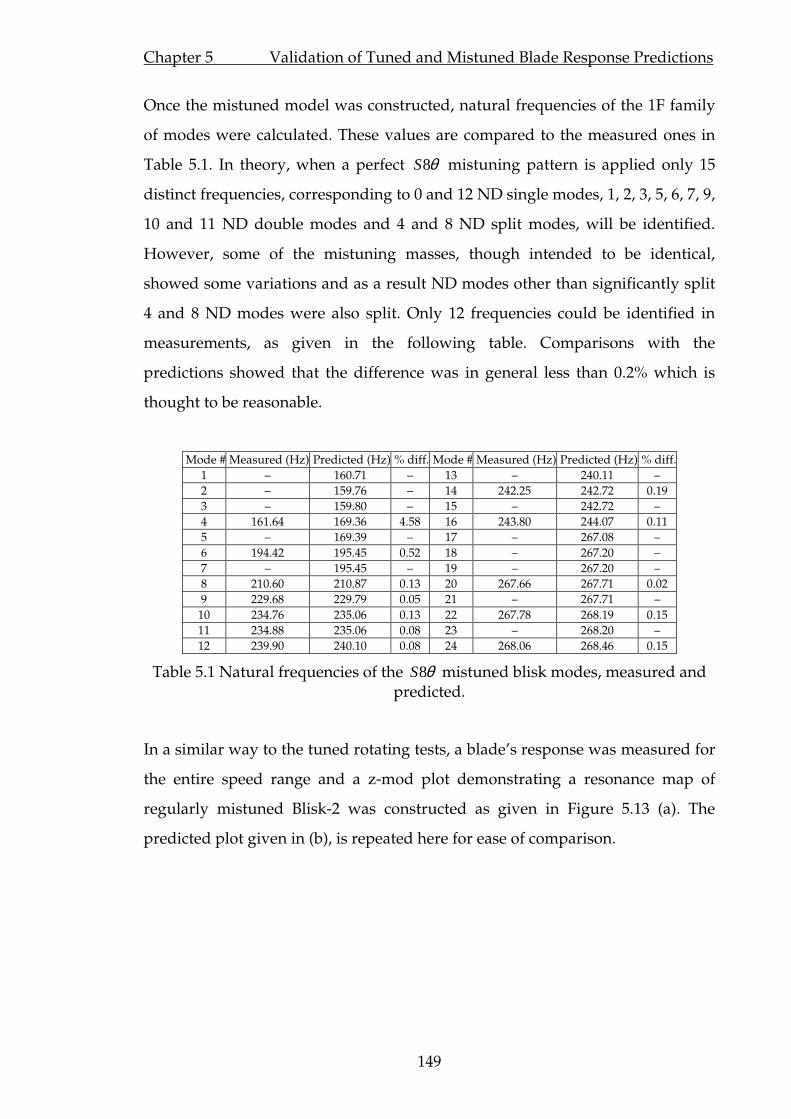
Chapter 5 Validation of Tuned and Mistuned Blade Response Predictions
149
Once the mistuned model was constructed, natural frequencies of the 1F family
of modes were calculated. These values are compared to the measured ones in
Table 5.1. In theory, when a perfect 8S θ mistuning pattern is applied only 15
distinct frequencies, corresponding to 0 and 12 ND single modes, 1, 2, 3, 5, 6, 7, 9,
10 and 11 ND double modes and 4 and 8 ND split modes, will be identified.
However, some of the mistuning masses, though intended to be identical,
showed some variations and as a result ND modes other than significantly split
4 and 8 ND modes were also split. Only 12 frequencies could be identified in
measurements, as given in the following table. Comparisons with the
predictions showed that the difference was in general less than 0.2% which is
thought to be reasonable.
Mode # Measured (Hz) Predicted (Hz) % diff. Mode # Measured (Hz) Predicted (Hz) % diff.
1 – 160.71 – 13 – 240.11 –
2 – 159.76 – 14 242.25 242.72 0.19
3 – 159.80 – 15 – 242.72 –
4 161.64 169.36 4.58 16 243.80 244.07 0.11
5 – 169.39 – 17 – 267.08 –
6 194.42 195.45 0.52 18 – 267.20 –
7 – 195.45 – 19 – 267.20 –
8 210.60 210.87 0.13 20 267.66 267.71 0.02
9 229.68 229.79 0.05 21 – 267.71 –
10 234.76 235.06 0.13 22 267.78 268.19 0.15
11 234.88 235.06 0.08 23 – 268.20 –
12 239.90 240.10 0.08 24 268.06 268.46 0.15
Table 5.1 Natural frequencies of the 8S θ mistuned blisk modes, measured and predicted.
In a similar way to the tuned rotating tests, a blade’s response was measured for
the entire speed range and a z-mod plot demonstrating a resonance map of
regularly mistuned Blisk-2 was constructed as given in Figure 5.13 (a). The
predicted plot given in (b), is repeated here for ease of comparison.
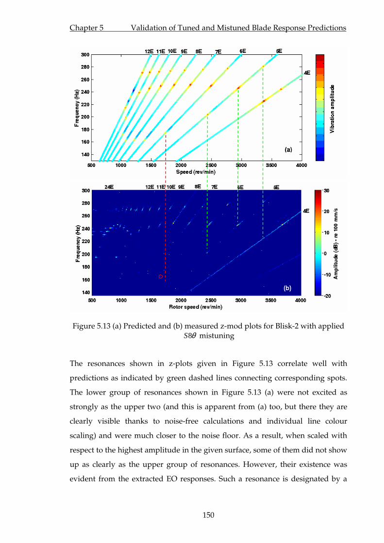
Chapter 5 Validation of Tuned and Mistuned Blade Response Predictions
150
Figure 5.13 (a) Predicted and (b) measured z-mod plots for Blisk-2 with applied 8S θ mistuning
The resonances shown in z-plots given in Figure 5.13 correlate well with
predictions as indicated by green dashed lines connecting corresponding spots.
The lower group of resonances shown in Figure 5.13 (a) were not excited as
strongly as the upper two (and this is apparent from (a) too, but there they are
clearly visible thanks to noise-free calculations and individual line colour
scaling) and were much closer to the noise floor. As a result, when scaled with
respect to the highest amplitude in the given surface, some of them did not show
up as clearly as the upper group of resonances. However, their existence was
evident from the extracted EO responses. Such a resonance is designated by a

Chapter 5 Validation of Tuned and Mistuned Blade Response Predictions
151
red circle (the lowest resonance on the 6EO line) in Figure 5.13 (b). The red
dashed line indicates that this resonance was excited at a lower speed in
measurements than it was in predictions. As explained in Chapter 4.4, the 6EO
line excited a predominantly 2ND mode at this resonance. Since the blisk fixing
in the test rig was not as rigid as the prediction tool assumed it was, the natural
frequencies of the modes at the lower end of 1F family of modes were (as they
are most affected by the disk boundary conditions) lower and excited at lower
speeds. Hence, this resonance was kept out of the speed range of individual
blade measurements. Similar to the tuned case, the lack of perfect alignment of
the LDV beam with the rotation axis manifested itself on 1, 2 and 4 EO lines (1
and 2 EO lines not shown). Resonances corresponding to the 1F family of modes
excited by higher EOs (13 and above), due to spatial aliasing, were also captured
in measurements and are clearly demonstrated on the given z-plot. Responses of
all blades to 6EO excitation were measured in the speed range of 2350-2850
rev/min, thus covering two prominent resonances shown in z-plots, as decided
in the test design phase. The results of these measurements are given in Figure
5.14.
Figure 5.14 Response of Blisk-2 with 8S θ mistuning to 6EO excitation - all blade measurements.

Chapter 5 Validation of Tuned and Mistuned Blade Response Predictions
152
Since a regular mistuning pattern consisting of three different masses was
applied (i.e. three masses periodically distributed round the blisk), blades
having the same mistuning mass should exhibit the same response. This was
demonstrated gratifyingly by the measurements and is more clearly seen from
the inset given in Figure 5.14. Although, in theory, measuring only three blades
would have sufficed, all blades were measured: (i) to prove that this behaviour
was confirmed by real data, and (ii) to have an envelope of variability through
multiple measurements of “identical” blades.
Measured individual blade responses given in Figure 5.14 were compared to
their predicted counterparts and are given in Figure 5.25.
235 240 245 250 255 260 265 270 275 280 285-40
-20
0
20
40
Frequency (Hz)
Am
plitu
de (
dB)
- re
100
mm
/s
MeasurementMISTRES
Blade # 1,4,7,...,22
235 240 245 250 255 260 265 270 275 280 285-40
-20
0
20
40
Frequency (Hz)
Am
plitu
de (
dB)
- re
100
mm
/s
MeasurementMISTRES
Blade # 2,5,8,...,23

Chapter 5 Validation of Tuned and Mistuned Blade Response Predictions
153
235 240 245 250 255 260 265 270 275 280 285-40
-20
0
20
40
Frequency (Hz)
Am
plitu
de (
dB)
- re
100
mm
/sMeasurementMISTRES
Blade # 3,6,9,...,24
Figure 5.15 Blisk-2 with 8S θ mistuning pattern: Comparison of individual blade
responses to 6EO excitation.
Similarly, due to the lightly damped nature of the blisk, the resonance peak
amplitudes could not be captured precisely, and were significantly different
than those predicted. However, away from the resonance regions the response
curves were strikingly similar to those predicted by the numerical model. Figure
5.16 shows close-up views of measured and predicted resonance groups shown
in Figure 5.15. As shown in Figure 5.16 (a), it is predicted that two very close
modes should be excited. However, this could not be seen from the measured
plots, primarily due to insufficient sweep rate (note that the minimum speed
increment was 1 rev/min, which meant that the frequency increments for the
6EO response measurements could not be less than 0.1 Hz). The same effect, to
an extent, is seen from Figure 5.16 (b) as well, where one of the small-amplitude
sharp resonances is not showing on the measured response curve. Also from
Figure 5.16 (b), a steady shift in frequency is apparent, though, in general, it is
around 0.1% and amplified, in this particular case, because of the narrow
frequency range shown. Nevertheless, the predicted response curves, both in
Figure 5.16 (a) and (b) are reassuringly followed by the measured data

Chapter 5 Validation of Tuned and Mistuned Blade Response Predictions
154
245 245.5 246 246.5 247 247.5 248 248.5 249-15
-10
-5
0
5
10
15
20
25
30
35
Frequency (Hz)
Am
plitu
de (
dB)
- re
100
mm
/s
274 275 276 277 278 279-30
-25
-20
-15
-10
-5
0
5
10
15
20
25
Frequency (Hz)
Group 1 Group 2
A
B
(a) (b)
Figure 5.16 Close-up of covered resonance groups Measured and predicted amplitude curves for blade #1.
Blade-to-blade response amplitude patterns for both of the resonance groups
were also compared with the predictions as shown in Figure 5.17. For this
purpose, using a slow-circular scan at the blade tips, all the blade amplitudes
were measured at frequency (speed) points A and B, as shown in Figure 5.16 (a)
and (b) respectively. The points A and B were selected as at around the
immediate neighbourhood of the resonances, true amplitude peaks could not be
measured due to truncated signals. It was demonstrated in Figure 5.11, that
uncertainties in the proximity of the selected speed point (e.g. A or B) to the true
resonance frequency lead to significant errors in amplitude comparisons. In
order to make sure that corresponding data are compared, the predicted
amplitude variation is amplitude-scaled such that one of the blade amplitudes
matches the measured counterpart. This is appropriate as it is already proved
through the given response curves that, away from the resonances, the
measured amplitudes are closely predicted in numerical simulations. Despite
minor departures, amplitude variation plots show good agreement both in terms
of distribution and amplitude. Extracted inter-blade phase angles corresponding
to given amplitude variations showed that standing waves were excited at both
measurement speeds.

Chapter 5 Validation of Tuned and Mistuned Blade Response Predictions
155
2 4 6 8 10 12 14 16 18 20 22 240
0.5
1
1.5
2
2 4 6 8 10 12 14 16 18 20 22 240
2
4
6
8
Blade #
Am
plitu
de (
V)
- 1V
= 1
00 m
m/s
MeasurementMISTRES(a)
(b)
Figure 5.17 Comparison of blade-to-blade amplitude variation at (a) point A, and (b) point B shown in Figure 5.16.
5.4.6 Randomly mistuned blisk analysis
The random mistuning pattern was obtained by “randomly” reshuffling the 8S θ
mistuning pattern, as explained in Chapter 4. Therefore, assuming that no
significant inherent mistuning existed in the blisk, the randomly-mistuned blisk
model to be used in predictions was obtained by simply changing the order of
the blades of the 8S θ model. Similarly, first the natural frequencies at rest were
measured, and the results are compared with the predictions in Table 5.2.
Mode # Measured (Hz) Predicted (Hz) % diff. Mode # Measured (Hz) Predicted (Hz) % diff.
1 - 157.97 - 13 239.40 239.80 0.17
2 - 160.08 - 14 248.25 248.73 0.19
3 - 160.85 - 15 248.50 248.82 0.13
4 161.70 169.54 4.63 16 251.80 252.20 0.16
5 162.70 170.97 4.84 17 262.80 263.25 0.17
6 194.05 195.13 0.55 18 265.75 265.40 0.13
7 196.64 197.97 0.67 19 266.10 265.79 0.12
8 214.55 214.97 0.20 20 267.85 267.90 0.02
9 221.20 221.61 0.18 21 268.10 267.92 0.07
10 227.30 227.67 0.16 22 268.40 268.50 0.04
11 232.75 233.11 0.15 23 269.80 269.81 0.00
12 235.40 235.72 0.14 24 271.40 271.45 0.02
Table 5.2 1F family natural frequencies of the randomly mistuned Blisk-2 at rest.

Chapter 5 Validation of Tuned and Mistuned Blade Response Predictions
156
Only 21 out of a possible 24 modes could be detected in the measured data.
Although an exceptionally good match was obtained for the natural frequencies
at the higher end of the 1F family of modes, the predictions in general departed
from measurements by 0.1 to 0.2%. Similar to the tuned and 8S θ cases, relatively
larger errors in the lower natural frequencies were probably due to flexibility of
the disk clamping in the experiments.
Before comparing individual response curves, it is useful, again, to see the
overall correspondence of the measurements and predictions using z-mod plots.
Such an experimental plot measured on blade 21 of the blisk and its predicted
counterpart are given in Figure 5.18.
Figure 5.18 Predicted and measured z-mod plots for Blisk-2 with applied random mistuning

Chapter 5 Validation of Tuned and Mistuned Blade Response Predictions
157
The vertical dashed green lines are provided to make the comparisons easier.
Overall, a very good correlation is observed between the given diagrams. Again,
due to global amplitude-dependent colour scaling in the measured plot, some of
the resonances were not seen as clearly as they were in the predicted one.
However they were evident on the extracted EO response curves.
Individual blade responses were measured for a speed range of 1400-1540
rev/min. This range covered 5 distinct resonance groups excited by 10EO
excitation. Extracted 10EO response curves are compared to the predicted ones
for all blades as given in Figure 5.19.
235 240 245 250 255-40
-30
-20
-10
0
10
20
30
235 240 245 250 255-60
-40
-20
0
20
235 240 245 250 255-60
-40
-20
0
20
40
(a) Blade # 1 (b) Blade # 2 (c) Blade # 3
235 240 245 250 255-40
-30
-20
-10
0
10
20
30
235 240 245 250 255-30
-20
-10
0
10
20
30
40
235 240 245 250 255-40
-20
0
20
40
60
(d) Blade # 4 (e) Blade # 5 (f) Blade # 6
235 240 245 250 255
-20
-10
0
10
20
30
40
50
1 2
3
235 240 245 250 255-40
-20
0
20
40
60
235 240 245 250 255-60
-40
-20
0
20
40
(g) Blade # 7 (i) Blade # 8 (j) Blade # 9
(Continued over…)
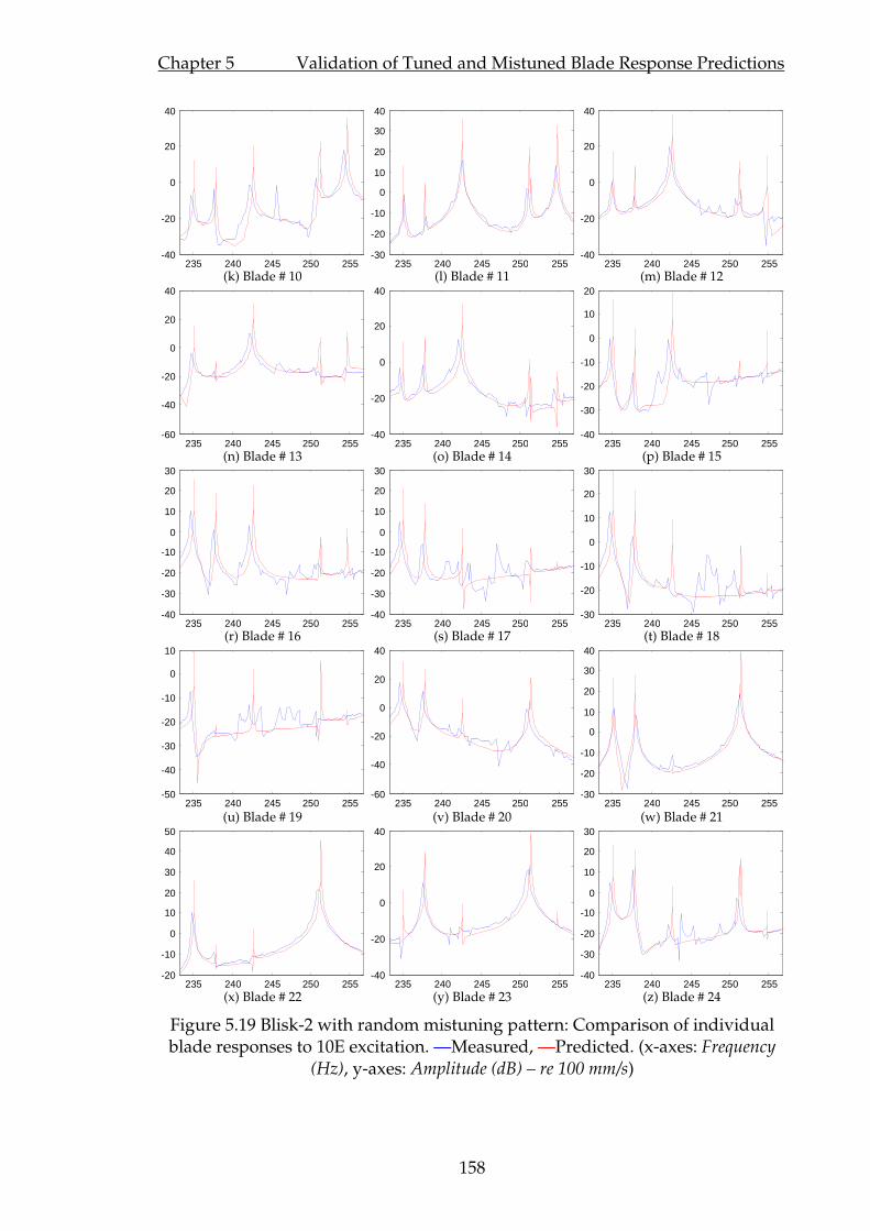
Chapter 5 Validation of Tuned and Mistuned Blade Response Predictions
158
235 240 245 250 255-40
-20
0
20
40
235 240 245 250 255-30
-20
-10
0
10
20
30
40
235 240 245 250 255-40
-20
0
20
40
(k) Blade # 10 (l) Blade # 11 (m) Blade # 12
235 240 245 250 255-60
-40
-20
0
20
40
235 240 245 250 255-40
-20
0
20
40
235 240 245 250 255-40
-30
-20
-10
0
10
20
(n) Blade # 13 (o) Blade # 14 (p) Blade # 15
235 240 245 250 255-40
-30
-20
-10
0
10
20
30
235 240 245 250 255-40
-30
-20
-10
0
10
20
30
235 240 245 250 255-30
-20
-10
0
10
20
30
(r) Blade # 16 (s) Blade # 17 (t) Blade # 18
235 240 245 250 255-50
-40
-30
-20
-10
0
10
235 240 245 250 255-60
-40
-20
0
20
40
235 240 245 250 255-30
-20
-10
0
10
20
30
40
(u) Blade # 19 (v) Blade # 20 (w) Blade # 21
235 240 245 250 255-20
-10
0
10
20
30
40
50
235 240 245 250 255-40
-20
0
20
40
235 240 245 250 255-40
-30
-20
-10
0
10
20
30
(x) Blade # 22 (y) Blade # 23 (z) Blade # 24
Figure 5.19 Blisk-2 with random mistuning pattern: Comparison of individual blade responses to 10E excitation. —Measured, —Predicted. (x-axes: Frequency
(Hz), y-axes: Amplitude (dB) – re 100 mm/s)
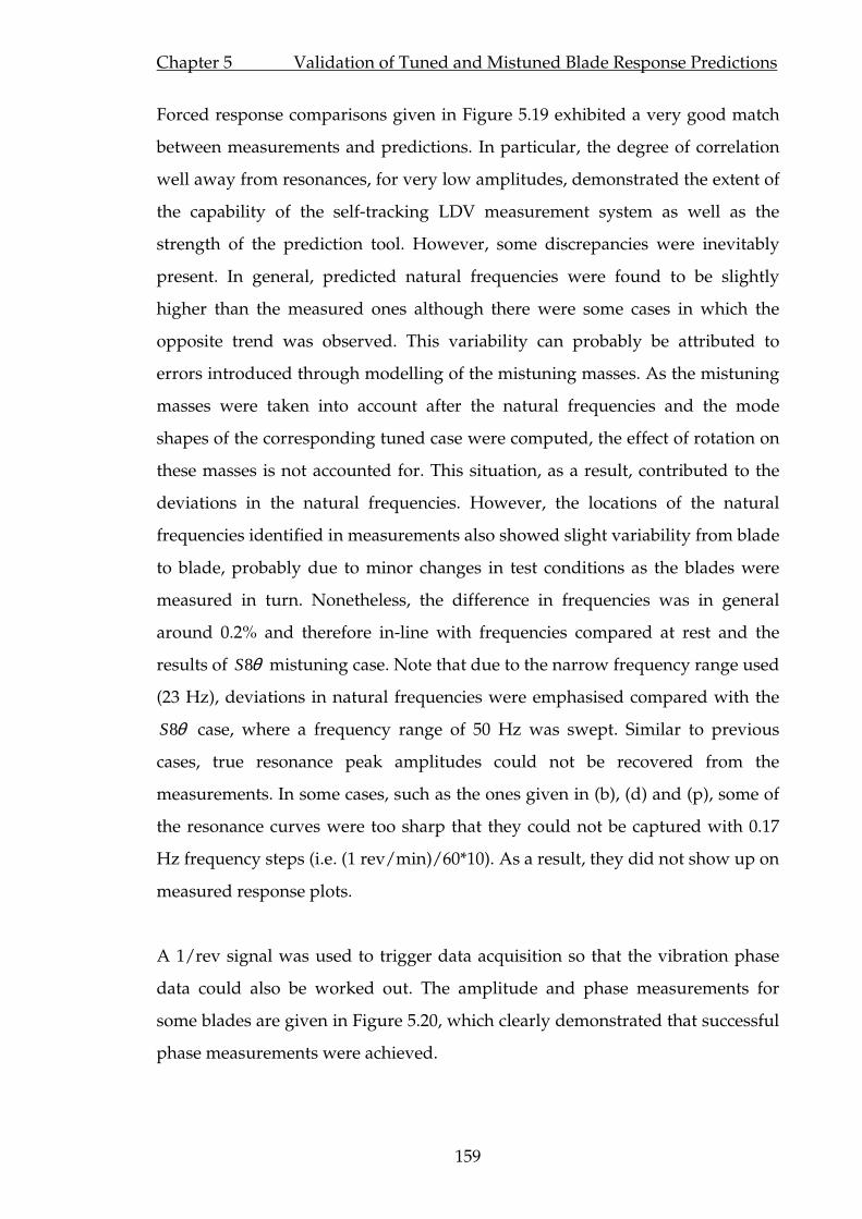
Chapter 5 Validation of Tuned and Mistuned Blade Response Predictions
159
Forced response comparisons given in Figure 5.19 exhibited a very good match
between measurements and predictions. In particular, the degree of correlation
well away from resonances, for very low amplitudes, demonstrated the extent of
the capability of the self-tracking LDV measurement system as well as the
strength of the prediction tool. However, some discrepancies were inevitably
present. In general, predicted natural frequencies were found to be slightly
higher than the measured ones although there were some cases in which the
opposite trend was observed. This variability can probably be attributed to
errors introduced through modelling of the mistuning masses. As the mistuning
masses were taken into account after the natural frequencies and the mode
shapes of the corresponding tuned case were computed, the effect of rotation on
these masses is not accounted for. This situation, as a result, contributed to the
deviations in the natural frequencies. However, the locations of the natural
frequencies identified in measurements also showed slight variability from blade
to blade, probably due to minor changes in test conditions as the blades were
measured in turn. Nonetheless, the difference in frequencies was in general
around 0.2% and therefore in-line with frequencies compared at rest and the
results of 8S θ mistuning case. Note that due to the narrow frequency range used
(23 Hz), deviations in natural frequencies were emphasised compared with the
8S θ case, where a frequency range of 50 Hz was swept. Similar to previous
cases, true resonance peak amplitudes could not be recovered from the
measurements. In some cases, such as the ones given in (b), (d) and (p), some of
the resonance curves were too sharp that they could not be captured with 0.17
Hz frequency steps (i.e. (1 rev/min)/60*10). As a result, they did not show up on
measured response plots.
A 1/rev signal was used to trigger data acquisition so that the vibration phase
data could also be worked out. The amplitude and phase measurements for
some blades are given in Figure 5.20, which clearly demonstrated that successful
phase measurements were achieved.

Chapter 5 Validation of Tuned and Mistuned Blade Response Predictions
160
230 235 240 245 250 255 2600
2
4
6
8
230 235 240 245 250 255 2600
2.5
5
7.5
10
230 235 240 245 250 255 2600
3
6
9
12
230 235 240 245 250 255 260-200
-100
0
100
200
Frequency (Hz)
Am
plitu
de (
V)
- 1V
= 1
00 m
m/s
230 235 240 245 250 255 260-200
-100
0
100
200
Frequency (Hz)230 235 240 245 250 255 260
-200
-100
0
100
200
Frequency (Hz)
Pha
se (d
eg)
(a) Blade # 8 (b) Blade # 22 (c) Blade # 23
Figure 5.20 Amp. and phase measurements for blades (a) 8, (b) 22, and (c) 23.
Some of the response plots, Figure 5.19 (a)-(d), (t), (u) etc., depicted resonances at
around 241, 244, 246 and 248 Hz which were not predicted by the numerical
simulations for 10EO excitation. However, as it is evident from the z-mod plots
given in Figure 5.18, that EOs 9 and 11, and to an extent 8, excited strong
resonances in the speed range of measurements, corresponding to these
frequencies for the mentioned blades. This was clearly seen from experimental
response curves extracted for these EO excitations. The contribution of 10EO
response was probably amplified due to large vibration amplitudes at
corresponding rotation speeds and manifested itself as spurious resonances.
Even so, their amplitudes were generally less than -10 dB. The response of blade
2 to 9, 10 and 11 EO excitations in the speed range of measurements is given in
Figure 5.21. Predicted response curves are also given.
1400 1420 1440 1460 1480 1500 1520 1540-60
-50
-40
-30
-20
-10
0
10
20
30
Rotor speed (rev/min)
Am
plitu
de (
dB)
- re
100
mm
/s
9EO - Exp.9EO - MISTRES10EO - Exp.10EO - MISTRES
1400 1420 1440 1460 1480 1500 1520 1540-40
-30
-20
-10
0
10
20
30
40
Rotor speed (rev/min)
Am
plitu
de (
dB)
- re
100
mm
/s
11EO - Exp.11EO - MISTRES10EO - Exp.10EO - MISTRES
(a) (b)
Figure 5.21 Response of blade 2 to 9, 10 and 11 EO excitations.
Chapter 5 Validation of Tuned and Mistuned Blade Response Predictions
161
It is seen from the above figures that 11EO excited strong resonances at 1462 and
1492 rev/min, and 9EO at 1447 and 1490 rev/min, although not as strongly. The
reflections of these resonances are clearly seen on the 10EO response curve.
Close inspection of the time histories of the corresponding data showed no clear
evidence of beating to suggest that two very close frequencies were excited. The
time data showed a dominant single vibration frequency. It is interesting here to
note that this phenomenon occurred only for the blades which were weakly
excited by 10EO and at the same time strongly excited by 9 or 11EO excitations.
All blade measurements were planned for a very small rotational speed range as
wider ranges demanded excessive measurement times. Although this range
covered a significant amount of data to asses the quality of the predictions, it
was thought appropriate to measure one particular blade with sufficiently fine
speed steps and for a wider range to make sure that predictions are inline with
measurements not only in a small range but also for a wider range. The best
candidate for this measurement was blade 21 as in construction of the z-mod
plot most of the data points were already available. For this particular
measurement, intermediate speed values were added to obtain a finer
resolution. The measured and predicted responses of blade 21 to 10EO excitation
are given in Figure 5.22 (a). The plotted curves present a striking similarity not
only at around resonances but also at around anti-resonances thus validating
both the prediction tool and the measurement setup. The response curves of this
blade to other EO excitations were also compared with the predictions and
similar results were obtained. So far, when plotting the measured response
curves, the actual measured data points were connected by solid lines visual
clarity. However, the accurate representation should have plotted them as
separate points, as shown in Figure 5.22 (b). This is necessary as experimental
curves are not complete, particularly around resonances, simply because there
are not enough measurement points to define the resonance peaks accurately
(see also Chapter 4, Section 4.4.1). Thus, the apparent difference between the
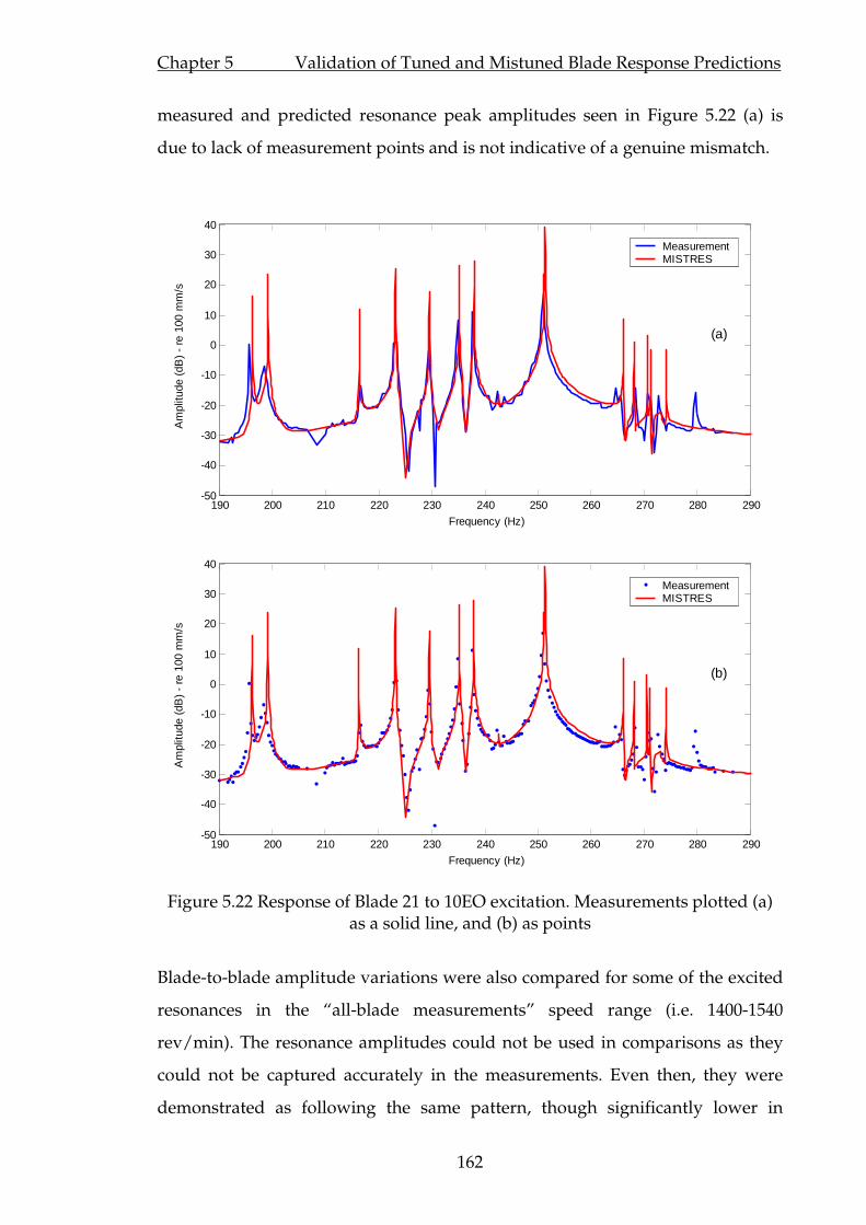
Chapter 5 Validation of Tuned and Mistuned Blade Response Predictions
162
measured and predicted resonance peak amplitudes seen in Figure 5.22 (a) is
due to lack of measurement points and is not indicative of a genuine mismatch.
190 200 210 220 230 240 250 260 270 280 290-50
-40
-30
-20
-10
0
10
20
30
40
Frequency (Hz)
Am
plitu
de (
dB)
- re
100
mm
/s
MeasurementMISTRES
(a)
190 200 210 220 230 240 250 260 270 280 290-50
-40
-30
-20
-10
0
10
20
30
40
Frequency (Hz)
Am
plitu
de (
dB)
- re
100
mm
/s
MeasurementMISTRES
(b)
Figure 5.22 Response of Blade 21 to 10EO excitation. Measurements plotted (a) as a solid line, and (b) as points
Blade-to-blade amplitude variations were also compared for some of the excited
resonances in the “all-blade measurements” speed range (i.e. 1400-1540
rev/min). The resonance amplitudes could not be used in comparisons as they
could not be captured accurately in the measurements. Even then, they were
demonstrated as following the same pattern, though significantly lower in
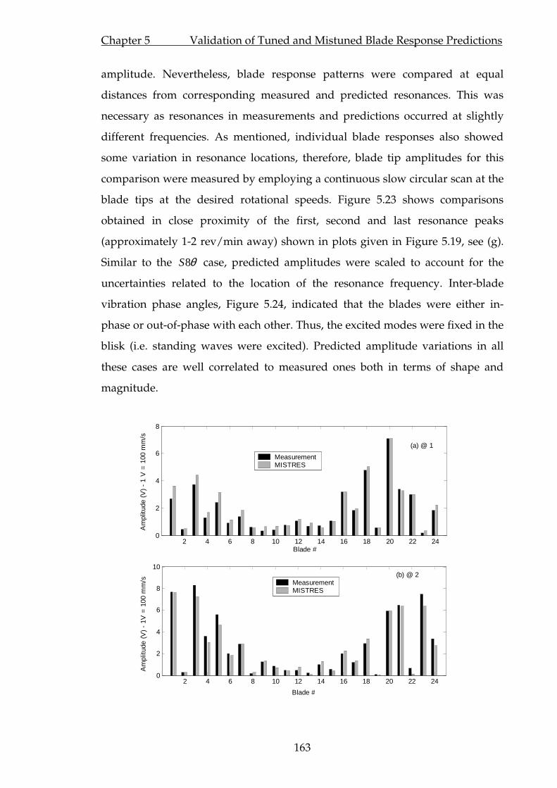
Chapter 5 Validation of Tuned and Mistuned Blade Response Predictions
163
amplitude. Nevertheless, blade response patterns were compared at equal
distances from corresponding measured and predicted resonances. This was
necessary as resonances in measurements and predictions occurred at slightly
different frequencies. As mentioned, individual blade responses also showed
some variation in resonance locations, therefore, blade tip amplitudes for this
comparison were measured by employing a continuous slow circular scan at the
blade tips at the desired rotational speeds. Figure 5.23 shows comparisons
obtained in close proximity of the first, second and last resonance peaks
(approximately 1-2 rev/min away) shown in plots given in Figure 5.19, see (g).
Similar to the 8S θ case, predicted amplitudes were scaled to account for the
uncertainties related to the location of the resonance frequency. Inter-blade
vibration phase angles, Figure 5.24, indicated that the blades were either in-
phase or out-of-phase with each other. Thus, the excited modes were fixed in the
blisk (i.e. standing waves were excited). Predicted amplitude variations in all
these cases are well correlated to measured ones both in terms of shape and
magnitude.
2 4 6 8 10 12 14 16 18 20 22 240
2
4
6
8
Blade #
Am
plitu
de (
V)
- 1
V =
100
mm
/s
MeasurementMISTRES
(a) @ 1
2 4 6 8 10 12 14 16 18 20 22 240
2
4
6
8
10
Am
plitu
de (
V)
- 1V
= 1
00 m
m/s
Blade #
MeasurementMISTRES
(b) @ 2

Chapter 5 Validation of Tuned and Mistuned Blade Response Predictions
164
2 4 6 8 10 12 14 16 18 20 22 240
1
2
3
4
5
6
Blade #
Am
plitu
de (
V)
- 1
V =
100
mm
/s
(c) @ 3
Figure 5.23 Comparison of blade-to-blade tip amplitude variations at various resonances excited by 10EO excitation.
2 6 10 14 18 22-50
0
50
100
150
200
Blade #
Inte
r-bl
ade
phas
e an
gle
(deg
ree)
2 6 10 14 18 22-200
-150
-100
-50
0
50
Blade #
(a) @ 1
(b) @ 2
Figure 5.24 Inter-blade phase angles corresponding to amplitude plots given in Figure 5.23 (a) and (b).
5.5. Summary
In this chapter the forced response predictions of the tuned and mistuned Blisk-
2, at rest and under rotating conditions have been validated through a
comprehensive test campaign using the testpiece (Blisk-2) and rig whose design
and development were reported earlier in the thesis. The validation strategy
adopted has been one in which a step is taken at a time to make sure that all
possible sources of uncertainties have been accounted for. Thus, the validation of
the following have been considered: (i) natural frequencies and mode shapes in
the absence of rotation, (ii) inclusion of rotational speed in the predictions, (iii)
modelling of mistuning masses, (iv) repeatability of measurements and

Chapter 5 Validation of Tuned and Mistuned Blade Response Predictions
165
reliability of the test setup, (v) response curves over wide speed ranges as well
as short ones, and (vi) peak responses (i.e. ODSs) in the presence of uncertainty
of actual damping levels.
First, the response prediction tool used in simulations was introduced. Its main
advantages and the way it models mistuning were explained. Following that, the
measured ODSs for the mistuned stationary blisk were compared with the
predicted ones and a very good match was obtained. Then, starting with the
tuned case, rotating test results with the applied regular and random mistuning
patterns were presented and corresponding predictions were overlaid. The
ability of the rig to reproduce the same data under the same conditions was
verified through a devised method involving shifted mistuning patterns.
Measured and predicted z-mod plots were demonstrated to be correlating very
well although the predictions of the some of the disk-dominated lower natural
frequencies were lower in measurements. In general, the predicted resonance
frequencies deviated from the measured ones by 0.2%. As a result of the very
low damping in the rig, the true resonance peak amplitudes could not be
measured. This was because; (i) the resonance peaks were very sharp that speed
increments much smaller than 1 rev/min (minimum available in the rig) were
needed to capture them accurately, and (ii) the peak amplitudes were so large
that the data acquisition board was overloading. However, away from the
resonance peaks, an exceptionally good agreement was obtained, in general,
between measured and predicted behaviour.
Blade-to-blade amplitude variations were also compared for the tuned and
mistuned cases. In the tuned case, travelling waves were excited resulting in all
blades having the same vibration amplitude, as predicted by theory. However,
in mistuned cases the modes were grossly localised and were fixed in the blisk.
Predicted patterns were illustrated to be perfectly verified in considerable detail
by measurements both in terms of shape and magnitude. The quality of the
match proved the vibration measurement rig as a well controlled environment

Chapter 5 Validation of Tuned and Mistuned Blade Response Predictions
166
and the non-contacting self-tracking LDV technique as an accurate way of
acquiring vibration response under rotation.

Chapter 6 Validation of Undamped and Damped Blade Response …
167
CHAPTER 6
VALIDATION of UNDAMPED and
DAMPED BLADE RESPONSE
PREDICTIONS
6.1 Overview
This chapter focuses on the evaluation of tests performed on Blisk-1 with
Cottage Roof dampers and assesses the validity of the forced response
predictions based on these tests. However, the undamped blisk response is
considered first to measure the degree of correlation in the absence of non-
linearity. The non-linear forced response prediction tool to be validated is
introduced next. Mistuning of Blisk-1, identified in Chapter 4 in terms of 1F
sector natural frequencies, is translated into physical mistuning and the effects of
different ways of performing the translation on the forced response are analysed.
Additionally, the consequences of variations in the amplitude of the forcing
input are discussed and the effects are shown using the Blisk-1 FE model.
6.2 The prediction tool
The development of the non-linear forced response prediction tool, and in
particular the modelling of the non-linear interfaces, to be validated in this study
is given in a series of papers, [37-39]. The application of the method to bladed
disks with friction and impact dampers can be found in reference [82]. Similarly,
the application of the method to mistuned bladed disks (mistuned through blade
properties and/or non-linear interface elements, i.e. friction dampers, gap values
etc.) can also be found in [40].
Chapter 6 Validation of Undamped and Damped Blade Response …
168
The main features of the method can be summarised as follows:
• use of multi-harmonic balance method in the solution of forced response
• applicability to any structure with the option to use cyclic symmetry for
structures exhibiting this property
• accurate description of friction forces in the presence of variable as well as
constant normal load;
• analytical formulation of contact interface elements, thus much faster
solution times, higher accuracy and rapid convergence.
Because of the above-mentioned features, the application of the method to
realistic industrial models with large DOFs and heavy non-linear behaviour,
resulting from under-platform and impact dampers, shroud contacts, gaps etc.
has been possible. The friction interface elements are used to describe the
interaction of surfaces in contact at a node; however, through use of many such
elements over a given area, modelling of complex surfaces in contact is also
possible. The method is coded into a computer program called FOrce Response
SuitE (FORSE), [87].
Figure 6.1 shows different stages in the formation of non-linear equations and
reduction process for a general, mistuned bladed disk application. System
matrices for the whole tuned bladed disk are formed from a sector model using
the method described in [14]. Through a multi-stage reduction technique, the
size of the non-linear equations is reduced to the number of the nodes where
non-linearities are applied. This enables the retained number of DOFs to be
several orders of magnitude less than total number of DOFs in the model.

Chapter 6 Validation of Undamped and Damped Blade Response …
169
Figure 6.1 Different stages in DOF reduction and formation of non-linear equations (Adapted from [40])
6.3 Frequency mistuning to physical mistuning
When Blisk-1 was received from the manufacturer, unlike Blisk-2, it was found
to be significantly mistuned. This inherent mistuning, despite some attempts,
could not be removed completely. Nevertheless, it was identified to a certain
degree in Chapter 4 as a sector-to-sector frequency deviation. As explained in
Chapter 5, frequency mistuning can be used as a direct input to the prediction
tool. However, it eventually needs to be represented by lumped mass or stiffness
elements. In doing so, the prediction tool varies the values of the assigned
mistuning masses or stiffnesses to adjust the natural frequencies of the first sub-
model (i.e. isolated blade or sector etc.) such that the provided natural frequency
mistuning is reproduced. Since only the first frequency of the sub-model is
considered, depending on the selection of mistuning nodes, assembly
characteristics other than the ones intended may be obtained, as discussed in
Chapter 4.2.3. In order to reduce the dependency of the resulting assembly
characteristics on the mistuning nodes, an isolated sector rather than a blade is
used as a sub-model. This yields two main benefits. First, since a bigger model is
used (a sector as opposed to a blade), matching only the first natural frequency
yields closer assembly characteristics. Secondly, the disk portion as well as the
blade is used to introduce mistuning and therefore a more realistic
representation is obtained.

Chapter 6 Validation of Undamped and Damped Blade Response …
170
However, despite these advantages, the location of mistuning nodes still bears
considerable importance. In Chapter 4, the blade-tip locations were found to be
the best choices for introducing mass mistuning. This was because the
characteristics of the whole assembly and sub-model were shown to be equally
sensitive to the changes brought in through these locations. However, the model
used in those calculations was a rather simple one. In order to analyse this effect
on a realistic model, mistuning was introduced at two distinct locations using
the Blisk-1 FE model. The configurations used are shown in Figure 6.2.
Figure 6.2 Introduction of mistuning in Blisk-1
For both configurations given in Figure 6.2, two sub-models: (i) isolated blade:
where the mistuning is defined as the variation of the 1F natural frequency of a
blade clamped at its root, and (ii) isolated sector: where the same variation is
defined in this case in terms of a sector model clamped at its cyclic symmetry
interfaces, were used. The errors introduced in the natural frequencies of the 1F
blisk modes for all possible configurations are given in Figure 6.3 where the bars
for each group present the deviations of obtained natural frequencies from the
measured ones at rest. For a given sub-model (blade and sector), for both ways
of introduction of mistuning (blade-tip and platform level), the first natural
frequencies of the individual models were exactly the same. It is seen from the
plot that the worst results were obtained when an isolated blade was used and
the mistuning was represented by nodes at platform level. However, when the
mistuning nodes were moved to the blade tip for the same sub-model, the error
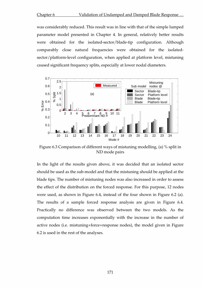
Chapter 6 Validation of Undamped and Damped Blade Response …
171
was considerably reduced. This result was in line with that of the simple lumped
parameter model presented in Chapter 4. In general, relatively better results
were obtained for the isolated-sector/blade-tip configuration. Although
comparably close natural frequencies were obtained for the isolated-
sector/platform-level configuration, when applied at platform level, mistuning
caused significant frequency splits, especially at lower nodal diameters.
10 11 12 13 14 15 16 17 18 19 20 21 22 23 240
0.1
0.2
0.3
0.4
0.5
0.6
0.7
Mode #
% E
rror
Sector Blade-tipSector Platform levelBlade Blade-tipBlade Platform level
2 3 4 5 6 7 8 9 10 110
0.5
1
1.5
2
2.5
Predominant ND #
% S
plit
Measured Sub modelMistuningnodes @
(a)
Figure 6.3 Comparison of different ways of mistuning modelling, (a) % split in ND mode pairs
In the light of the results given above, it was decided that an isolated sector
should be used as the sub-model and that the mistuning should be applied at the
blade tips. The number of mistuning nodes was also increased in order to assess
the effect of the distribution on the forced response. For this purpose, 12 nodes
were used, as shown in Figure 6.4, instead of the four shown in Figure 6.2 (a).
The results of a sample forced response analysis are given in Figure 6.4.
Practically no difference was observed between the two models. As the
computation time increases exponentially with the increase in the number of
active nodes (i.e. mistuning+force+response nodes), the model given in Figure
6.2 is used in the rest of the analyses.

Chapter 6 Validation of Undamped and Damped Blade Response …
172
285 286 287 288 289 290 291 292 293
-30
-20
-10
0
10
20
30
Frequency (Hz)
Am
plitu
de (
dB)
12 Nodes4 Nodes
Figure 6.4 Introduction of mistuning through different number of nodes
6.4 Effects of excitation and mistuning errors on the forced
response
6.4.1 Excitation errors
During the tuning process for Blisk-1, a significant amount of metal was
removed from the blade tips. This implied that the magnet force applied on each
blade might somehow be different, resulting in a variable amplitude forcing
input around the blisk during its operation. In order to account for the effect of
this variation, a recorded magnet signal was analysed to quantify the degree of
variability. Such a signal is given in Figure 6.5.
0 0.2 0.4 0.6 0.8 1 1.2 1.4 1.6 1.8 20
5
10
15
Time (s)
Am
plitu
de (
N)
Magnet signalTrigger signal
1 rotation
Figure 6.5 A typical magnet force signal applied to Blisk-1
Ideally, each pulse given in Figure 6.5 should have had the same amplitude.
However, as expected in this case, the force signal presented a variation from

Chapter 6 Validation of Undamped and Damped Blade Response …
173
blade-to-blade (note that each pulse corresponds to a blade). It is seen that the
peak amplitudes of pulses generated for each blade are slightly different and the
pattern of variation repeats itself in each rotation cycle, as demonstrated in
Figure 6.6 (a). In order to understand this better, these amplitudes are plotted in
a circular form on a 3-D graph and given in Figure 6.6 (b).
2 4 6 8 10 12 14 16 18 20 22 2414.6
14.8
15
15.2
15.4
15.6
15.8
16
16.2
16.4
16.6
Am
plitu
de (N
)
Blade #
Rotation 1Rotation 2
Correlation coef. = 99.5% Mean Force = 14.42 N Scatter = 1.85 NStandart Dev. = 0.44Max. dev. from mean = 6.6 %
(a)
Figure 6.6. Variation of peak magnet force applied to blades of Blisk-1.
The pattern of variation given in Figure 6.6 did not correlate to the pattern
formed by the amount of removed metal. The deviation of the peak amplitudes
from the plane of the mean value (indicated by the flat circular area) given in
Figure Figure 6.6 (b) suggested that the bladed disk was not perpendicular to the
axis of rotation but tilted (i.e., swash error). Since tapered-lock devices were
used to secure the bladed disk to the shaft (note that this was not the case for
Blisk-2 as a different clamping mechanism was used), the degree of control on
perpendicularity was somewhat limited. Additionally, it is thought that the
drive shaft was slightly bent in the process of aligning the balancing disk with
the identified mark on the blisk, a process which necessitated high forces to be
applied to the drive shaft. In addition, it must be noted that some of the blades
might have had slightly different stagger angles or bent, in a way to amplify this
variation. These errors, combined with the effects due to different blade masses,
are thought to have caused the presented variation.
Correlation coef. = 99.5% Mean Force = 15.42 N Scatter = 1.85 N Standard Dev. = 0.44 Max dev. From mean = 6.6%

Chapter 6 Validation of Undamped and Damped Blade Response …
174
6.4.2 Analysis of excitation errors
The effects of EO excitation errors (i.e. each blade receiving a slightly different
force amplitude) was investigated on Blisk-1 FE model. For this purpose, two
travelling wave excitations, one having constant amplitude (the mean value of
the variation) and the other having the exact variation given in Figure 6.6, were
considered. The errors in the excitation phase were neglected, based on the
speed measurements given in Chapter 3, as the blade arrival times were very
consistent. For both excitation patterns, the Fourier coefficients of the magnet
pulses were calculated as described in Chapter 5. Note that for the second case
these coefficients needed to be calculated for all 24 pulses separately. The
variation of 9th harmonic’s amplitude is plotted in Figure 6.7 (a), as an example.
The calculations were repeated both in the presence and absence of physical
mistuning. The mistuned response prediction tool used in calculations,
MISTRES, did not allow the amplitude of the applied EO excitation force to be
different for different blades. Therefore, a commercially available FE package, in
this case ANSYS, was used in calculations. This meant that a cyclic sector could
not be utilised anymore. Therefore, a full blisk FE model was used. However,
performing detailed forced response analyses in ANSYS proved to be extremely
costly in terms of computation times. For this purpose, only the mode shapes
and the natural frequencies were calculated (first 6 families of modes) using this
package and the forced response was performed by a code written in Matlab.
This way, the response was calculated for the nodes of interest, and much faster
solution times and higher frequency resolutions were possible. The response of a
particular blade obtained for both cases (i.e. tuned and mistuned) when
subjected to 9EO excitation are given in Figure 6.7 (b). Although the bladed disk
model used in (b-1) was perfectly tuned, the green curve exhibits response
characteristics of a mistuned bladed disk. As explained earlier in Chapter 2, in
order for a ND mode to be excited, the shapes of the excitation and the mode
excited, as well as their frequencies should match. When the amplitude of the
excitation varies, it contains some other harmonics, depending on the variation,
which eventually excite corresponding ND modes. However, unlike mistuning,

Chapter 6 Validation of Undamped and Damped Blade Response …
175
the uneven distribution of the EO excitation force amplitudes does not cause
double modes to split or change their natural frequencies. In the example given
in Figure 6.7 (b-1), the random case excited all ND modes covered in the
frequency range. Unlike physical mistuning, though, the force amplitude
variation did not cause any significant change in the forced response amplitude
of the main resonance (i.e. 9ND mode). For ±5% variation of the force amplitude,
the maximum increase in the response amplitude was less than 0.13%. In fact,
with ±5% force amplitude variation, the magnitude of the 6th harmonic did not
change much, thus causing little change in the response amplitude. Similar
results were obtained when a mistuned Blisk-1 model was used, as given in
Figure 6.7 (b). Here the shape of the response curve for the variable-amplitude
force case is not drastically different from the constant-amplitude one. This is
because all the modes are already excited by the employed EO excitation, thanks
to the now-finite-amplitude 9th harmonics present in their mode shapes. Even
then, the effect of force amplitude variation on the response amplitude is much
greater at the resonances, other than the main one, with variations up to 25%.
Similar deviations are also evident away from the resonance peaks though
increase in maximum amplitude for the given case is, likewise, less than 0.13%.
2 4 6 8 10 12 14 16 18 20 22 240.42
0.43
0.44
0.45
0.46
0.47
Blade #
9-E
O F
orc
e (N
)
Variable amp. forceConstant amp. force
Max. dev. from mean = 4.84%Standard dev = 0.0119
(a)

Chapter 6 Validation of Undamped and Damped Blade Response …
176
281 282 283 284 285 286 287 288-10
0
10
20
30
40
50
Frequency (Hz)
Am
plitu
de (
dB)
- re
100
mm
/s
Tuned - w/o excitation errorTuned - w/ excitation error
281 282 283 284 285 286 287 288-10
0
10
20
30
40
50
Frequency (Hz)
Misuned - w/o excitation errorMistuned - w/ excitation error
0
10
20
7ND
8ND
9ND
10ND 11ND
12ND
0.13%
0.13% 25%
(b-2) (b-1)
2 4 6 8 10 12 14 16 18 20 22 2444
46
48
50
52
Am
plitu
de (
dB)
- re
100
mm
/s w/o excitation error w/ excitation error
2 4 6 8 10 12 14 16 18 20 22 24
-0.2
-0.1
0
0.1
Blade #
% D
evia
tion
% Deviation
(c)
Figure 6.7(a) Applied force distributions, (b) forced response of blade 1, and (c) maximum blade-tip forced response amplitude comparison for mistuned Blisk-1.
The individual cases given in the above figure are important in providing a
comparison of the overall response curves in a given frequency range. However,
they alone do not present a true indication of the likely deviations the force
variation might cause. In order to get a better idea about this, a large number of
randomly varying force input shapes needed to be considered to form a
statistical basis. To this end, 10.000 randomly generated cases were considered.
Random vectors are chosen from a uniform distribution from the interval [0.0
1.0] and then shifted and scaled to provide a 5% variation on the mean value of
the force variation given in Figure 6.6. The results obtained for physically tuned
and mistuned bladed disk models are given in Figure 6.8. In both cases the
maximum amplification due to random variations is found to be similar, and
less than 3%. The maximum scatter in both cases is around 5%, although the

Chapter 6 Validation of Undamped and Damped Blade Response …
177
scatter in the mistuned case is slightly larger. The same calculations are repeated
for 6 and 11EO excitations as well, and similar results obtained.
0 2000 4000 6000 8000 100000.97
0.98
0.99
1
1.01
1.02
1.03
1.04
Case number
Nor
mal
ised
am
plitu
de -
A/A
cons
tant
Random variationConstant amplitude
0 2000 4000 6000 8000 100000.97
0.98
0.99
1
1.01
1.02
1.03
1.04
Case number
(a) (b)
Figure 6.8 Statistical variation of maximum 9EO response amplitude due to excitation errors on the (a) tuned and (b) mistuned Blisk-1 FE model.
When blade-to-blade maximum amplitude variations or response curve
comparisons at or around a given resonance are of interest, the excitation errors
can be considered negligible by comparison with the uncertainties involved in
the measurement system. However, for overall response curve comparisons, the
variation in the force amplitudes might have a greater effect and should be
remembered when assessing the correlation between predictions and
measurements. Although an imperfect excitation causes several modes of a
tuned system to be excited, its effects are not comparable with those of physical
mistuning in any way. The latter is known to yield amplitudes which are several
times larger than those of the corresponding tuned reference case. For example,
the amplitudes of non-9D resonances excited in the case shown in Figure 6.7 (b-
1) are much smaller than the corresponding mistuned amplitudes given in
Figure 6.7 (b-2). Based on the evidence provided, the effects of excitation errors
are considered insignificant and the mean value of the force was chosen for the
forced response calculations of this study.

Chapter 6 Validation of Undamped and Damped Blade Response …
178
6.4.3 Mistuning errors
The effects of possible errors in the mistuning pattern (i.e. combined errors,
originating from the identification process and those introduced in its
modelling) on forced response levels were analysed using the discrete bladed
disk model introduced in Chapter 4. This was appropriate as a qualitative
indication was needed and this simple model provided computational
efficiency. Here it was assumed that the overall trend of the mistuning variation
was identified reasonably accurately. To this end, the mistuning pattern
identified for Blisk-1 was perturbed randomly by ±10%, Figure 6.9 (a), and the
variation in the maximum forced response for 6EO excitation was calculated for
10000 cases. The random variations were, again, obtained from a normal
distribution. The deviations of the calculated maximum responses from the
maximum response due to the original mistuning pattern are shown in Figure
6.9 (b). It is seen that the increases due to uncertainties in mistuning pattern are
of the same order as those due to excitation errors. The fact that ±10% variation
in the mistuning pattern caused a maximum response amplification of just 1.3%
suggests that, (provided that the real error in mistuning pattern is not larger) the
errors involved in the identified pattern should not have a significant effect on
the correlation of the predictions and measurements.
0 2000 4000 6000 8000 100000.97
0.98
0.99
1
1.01
1.02
1.03
Nor
mal
ised
am
plitu
de -
A/A
ref
Case number
Perturbed patternsReference mistuning pattern
2 4 6 8 10 12 14 16 18 20 22 240.97
0.98
0.99
1
1.01
1.02
1.03
Blade number
Nor
mal
ised
am
plitu
de -
mm
istu
ned/m
tune
d
Error bars - 10%Reference mistuning pattern
(a) (b)
Figure 6.9 (a) Error in mistuning pattern, (b) Maximum forced response variation of a discrete bladed disk model due to errors in mistuning pattern

Chapter 6 Validation of Undamped and Damped Blade Response …
179
6.5 Undamped, rotating Blisk-1 analysis
Forced response analyses of undamped (i.e. the case of no additional damping
other than material damping) Blisk-1 were particularly important for the reason
that they would provide useful data to assess the suitability of the updated
model prior to non-linear analyses. The mistuned forced response prediction
tool was validated in Chapter 5 using measurements taken from Blisk-2.
Therefore, in the case of Blisk-1, uncertainties were likely to arise due to
inaccuracies in mistuning identification or in its representation, and, to an
extent, due to excitation errors.
6.5.1 Comparison of overall characteristics
Similar to the Blisk-2 response measurements, the first step here was to measure
the response of a particular blade over the entire speed range (i.e. 0-4000
rev/min). This, likewise, allowed the overall characteristics to be mapped out
and compared with the predicted ones on a general scale, as given in Figure 6.10.

Chapter 6 Validation of Undamped and Damped Blade Response …
180
Figure 6.10 (a) Computed and (b) measured interference diagrams on blade 1 of the undamped Blisk-1
Due to the mistuned nature of Blisk-1, the kth EO line excited a number of modes
depending on the magnitude of the kth harmonic in the mode shape of each.
Some of the resonance spots, or groups of resonances (in general the top group
of red spots contain very close many resonances), are interconnected via dashed
lines, indicating a good match.
It is seen from the measured z-mod plot that the effect of misalignment between
the laser beam and axis of rotation has deteriorated compared with the Blisk-2
case, as indicated by the emphasised EO lines. Most significantly, 1, 2, 4 and 8
EO responses are heavily affected. Although not on the same scale, other low EO
(a)
(b)
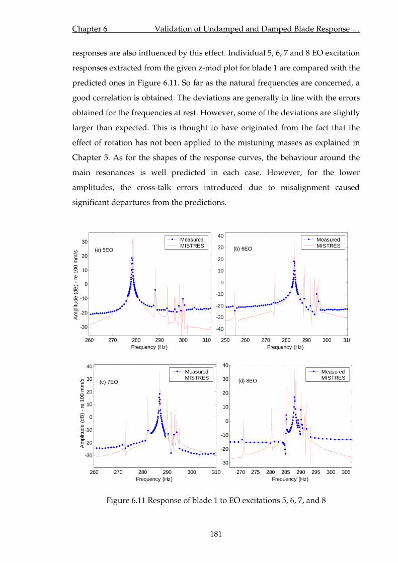
Chapter 6 Validation of Undamped and Damped Blade Response …
181
responses are also influenced by this effect. Individual 5, 6, 7 and 8 EO excitation
responses extracted from the given z-mod plot for blade 1 are compared with the
predicted ones in Figure 6.11. So far as the natural frequencies are concerned, a
good correlation is obtained. The deviations are generally in line with the errors
obtained for the frequencies at rest. However, some of the deviations are slightly
larger than expected. This is thought to have originated from the fact that the
effect of rotation has not been applied to the mistuning masses as explained in
Chapter 5. As for the shapes of the response curves, the behaviour around the
main resonances is well predicted in each case. However, for the lower
amplitudes, the cross-talk errors introduced due to misalignment caused
significant departures from the predictions.
260 270 280 290 300 310
-30
-20
-10
0
10
20
30
Frequency (Hz)
Am
plitu
de (
dB)
- re
100
mm
/s
MeasuredMISTRES
250 260 270 280 290 300 310
-40
-30
-20
-10
0
10
20
30
40
Frequency (Hz)
MeasuredMISTRES
(a) 5EO (b) 6EO
260 270 280 290 300 310
-30
-20
-10
0
10
20
30
40
Frequency (Hz)
Am
plitu
de (d
B) -
re 1
00 m
m/s
MeasuredMISTRES
270 275 280 285 290 295 300 305
-30
-20
-10
0
10
20
30
40
Frequency (Hz)
MeasuredMISTRES
(c) 7EO (d) 8EO
Figure 6.11 Response of blade 1 to EO excitations 5, 6, 7, and 8

Chapter 6 Validation of Undamped and Damped Blade Response …
182
The very light damping in Blisk-1 resulted in very sharp resonances peaks.
Thanks to an insufficient sweep rate, some of these could not be captured. The
measured amplitude and phase response curves were analysed in ICATS
software to determine the structural damping. However, the obtained damping
values under rotation and in vacuum were, surprisingly, significantly higher
than those measured at rest, in the presence of air. It was realised that this was
caused by the fact that the double ND modes were slightly split and therefore
could not be accurately distinguished in the measurements. As a result, very
close resonances were merged together and were processed as a single mode.
Naturally, the resulting damping values were misleadingly high. Following the
example of Blisk-2, and the fact that the same damping values were identified
for both blisks at rest, the same damping value (i.e. 0.0075%) was chosen for
Blisk-1 predictions under rotation.
6.5.2 Comparison of all blade responses
All the blades of the undamped Blisk-1 were chosen to be measured at around
the 9EO-9ND resonance. This required a speed range of 1900-1950 rev/min to be
covered. Despite being a very short range, it covered 9 resonances within a band
of 7.5 Hz, which would provide enough data to gauge the quality of the
mistuned predictions. The results of these measurements are compared to the
predicted ones and given in Figure 6.12. Only the odd numbered blades are
given for brevity.
286 288 290 292-20
-10
0
10
20
30
286 288 290 292-30
-20
-10
0
10
20
30
286 288 290 292-30
-20
-10
0
10
20
30
40
(a) Blade #1 (b) Blade #3 (c) Blade #5
(Continued over…)

Chapter 6 Validation of Undamped and Damped Blade Response …
183
286 288 290 292-40
-30
-20
-10
0
10
20
30
8D 9D
10D
11D
12D
286 288 290 292-20
-10
0
10
20
30
40
286 288 290 292-30
-20
-10
0
10
20
30
40
(d) Blade #7 (e) Blade #9 (f) Blade #11
286 288 290 292-30
-20
-10
0
10
20
30
40
286 288 290 292-30
-20
-10
0
10
20
30
40
286 288 290 292-60
-40
-20
0
20
40
(g) Blade #13 (h) Blade #15 (i) Blade #17
286 288 290 292-30
-20
-10
0
10
20
30
286 288 290 292-30
-20
-10
0
10
20
30
40
286 288 290 292-30
-20
-10
0
10
20
30
40
(j) Blade #19 (k) Blade #21 (l) Blade #23
Figure 6.12 Undamped Blisk-1: Comparison of individual blade responses to 9EO excitation. —Measured, —Predicted. (x-axes: Frequency (Hz), y-axes:
Amplitude (dB) – re 100 mm/s)
Although the match between the measurements and the predictions was not as
startling as the Blisk-2 results were, given the fact that a very small frequency
range was considered and the knowledge that inherent mistuning was not as
accurate, the overall characteristics and the general behaviour of the response
curves are well predicted. The deviations in the locations of the resonances were
generally around 0.1%. However, the predictions of the 12ND mode, in
particular, differed by up to 0.3% from the measurements, as seen from Figure
6.12 (d). The given plots also show that the frequency splits in 8, 10 and 11ND
modes were over predicted as was also evident from the inset of Figure 6.3. The
actual split mode pairs corresponding to these modes were so close that they
could not be measured as clearly as the 9ND mode pair. The resonance locations

Chapter 6 Validation of Undamped and Damped Blade Response …
184
obtained through measurements also showed some variability. This was
probably due to changes in test conditions as the blades were, again, measured
in turn, over a number of days. Thanks to the narrow frequency range, these
differences are accentuated.
6.5.3 Comparison of ODSs
During the testing of Blisk-1 at rest, it was observed that the lower ND modes,
although occurring in split pairs, maintained their regular sinusoidal shapes.
Therefore, all blades when excited at corresponding resonances would have
similar amplitudes, thus exhibiting tuned characteristics. This was also observed
from the ODSs measured on the rotating blisk. Some of these measurements are
compared with the predicted ones in Figure 6.13. The ODSs shown here were
measured by running the rig at the corresponding resonance speeds and then
measuring the blade-tip responses, either by a slow circular scan at the blade-
tips or by indexing the laser beam from blade to blade. Both methods were
demonstrated to have given the same results.
0 5 10 15 20 250
5
10
15
20
25
Blade #
Am
plitu
de (d
B) -
re
100
mm
/s
MeasuredMISTRES
5 10 15 20-200
-150
-100
-50
0
50
100
150
200
Inte
r-bl
ade
phas
e an
gle
(deg
ree)
Blade #
Measured
Blade#1Blade#2
(a) - 5ND mode excited by 5EO
ΩODS
5 10 15 200
2
4
6
8
10
12
14
16
18
20
Blade #
Am
plitu
de (d
B) -
re
100
mm
/s
2 4 6 8 10 12 14 16 18 20 22 24-150
-100
-50
0
50
100
150
Blade #
Inte
r-bl
ade
phas
e an
gel (
deg)
Measured
Odd bladesEven blades
(b) - 6ND mode excited by 6EO
ΩODS

Chapter 6 Validation of Undamped and Damped Blade Response …
185
0 5 10 15 20 250
1
2
3
4
5
6
Blade #
Am
plitu
de (
V)
- 1V
= 1
00 m
m/s
0 5 10 15 20 25-150
-100
-50
0
50
100
Blade #
Inte
r-bl
ade
phas
e an
gle
(deg
ree)
Measured
all baldes(c) - 9ND mode excited by 9EO Ω
ODS
Figure 6.13 Measured and predicted ODSs for (a) 5, (b) 6, and (c) 9ND modes excited by 5, 6, and 9EOs respectively.
The frequencies at which the response amplitudes were compared in the given
plots are indicated by ODSΩ in the insets, which show predicted blade responses
at around the corresponding ND mode pair. Inter-blade phase angle plots
indicated that 5 EO and 6 EO excitations excited travelling 5 and 6 ND modes
respectively, whereas 9EO excitation excited predominantly a 9ND mode with
both standing and travelling wave components. Measured and predicted
response patterns given in Figure 6.13 (a) and (b) correlate reasonably well.
Although larger deviations in amplitude and shape are evident for the ODS
corresponding to 9ND mode given in (c), in general a similar pattern is
observed. As is seen from the blade amplitude variations, the 9ND mode is
significantly mistuned and the errors involved in the identified mistuning and,
to an extent, in its modelling, are thought to have been responsible for the
deviations mentioned.
6.6 Damped, rotating Blisk-1 analyses
For the friction damped cases, Blisk-1 was fitted with Cottage-Roof (C-R) type
dampers as shown in Figure 6.14. Two sets of C-R dampers, one made of steel
and another from a titanium alloy were manufactured to provide a range of
damper masses. The variation of individual damper masses for both sets is given
in Table 6.1.
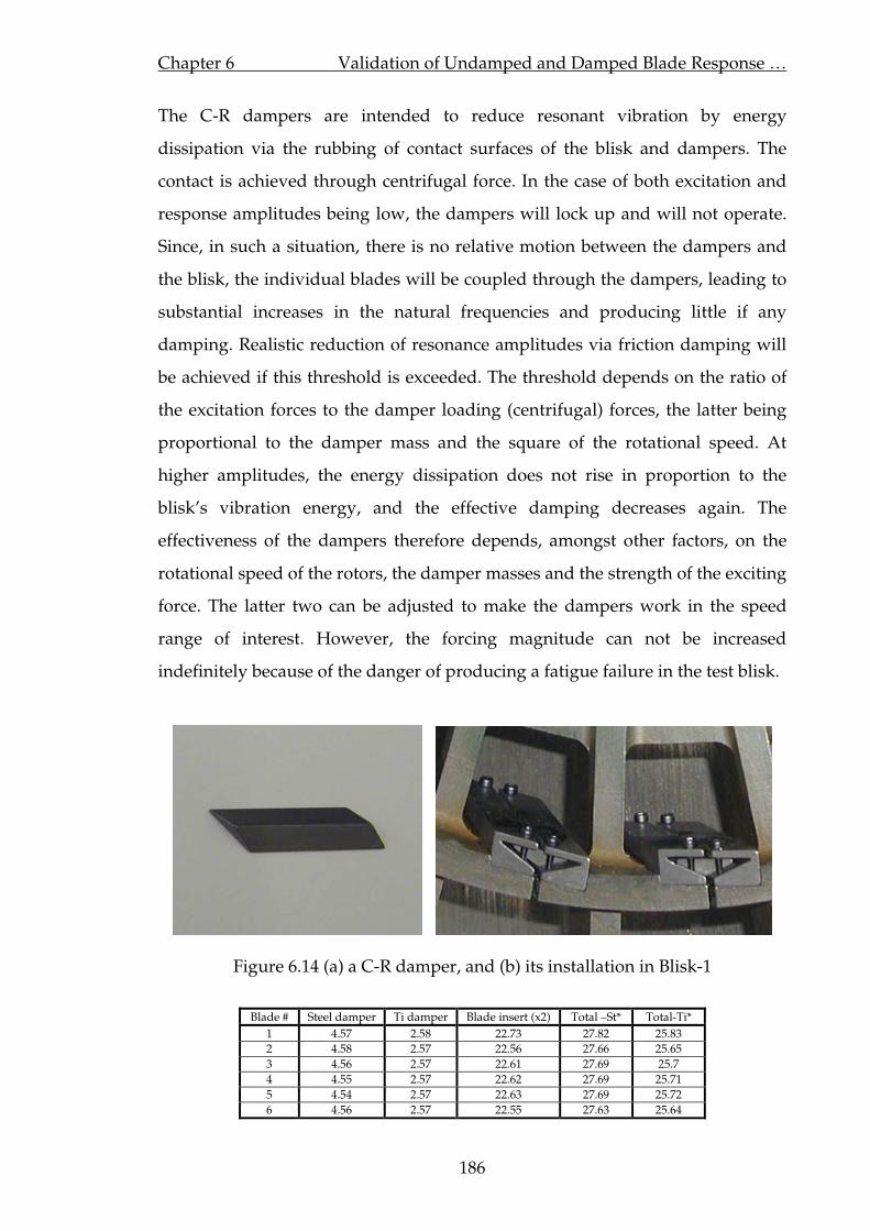
Chapter 6 Validation of Undamped and Damped Blade Response …
186
The C-R dampers are intended to reduce resonant vibration by energy
dissipation via the rubbing of contact surfaces of the blisk and dampers. The
contact is achieved through centrifugal force. In the case of both excitation and
response amplitudes being low, the dampers will lock up and will not operate.
Since, in such a situation, there is no relative motion between the dampers and
the blisk, the individual blades will be coupled through the dampers, leading to
substantial increases in the natural frequencies and producing little if any
damping. Realistic reduction of resonance amplitudes via friction damping will
be achieved if this threshold is exceeded. The threshold depends on the ratio of
the excitation forces to the damper loading (centrifugal) forces, the latter being
proportional to the damper mass and the square of the rotational speed. At
higher amplitudes, the energy dissipation does not rise in proportion to the
blisk’s vibration energy, and the effective damping decreases again. The
effectiveness of the dampers therefore depends, amongst other factors, on the
rotational speed of the rotors, the damper masses and the strength of the exciting
force. The latter two can be adjusted to make the dampers work in the speed
range of interest. However, the forcing magnitude can not be increased
indefinitely because of the danger of producing a fatigue failure in the test blisk.
Figure 6.14 (a) a C-R damper, and (b) its installation in Blisk-1
Blade # Steel damper Ti damper Blade insert (x2) Total –St* Total-Ti*
1 4.57 2.58 22.73 27.82 25.83
2 4.58 2.57 22.56 27.66 25.65
3 4.56 2.57 22.61 27.69 25.7
4 4.55 2.57 22.62 27.69 25.71
5 4.54 2.57 22.63 27.69 25.72
6 4.56 2.57 22.55 27.63 25.64
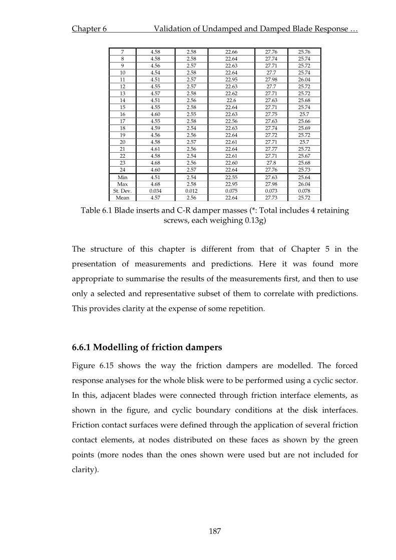
Chapter 6 Validation of Undamped and Damped Blade Response …
187
7 4.58 2.58 22.66 27.76 25.76
8 4.58 2.58 22.64 27.74 25.74
9 4.56 2.57 22.63 27.71 25.72
10 4.54 2.58 22.64 27.7 25.74
11 4.51 2.57 22.95 27.98 26.04
12 4.55 2.57 22.63 27.7 25.72
13 4.57 2.58 22.62 27.71 25.72
14 4.51 2.56 22.6 27.63 25.68
15 4.55 2.58 22.64 27.71 25.74
16 4.60 2.55 22.63 27.75 25.7
17 4.55 2.58 22.56 27.63 25.66
18 4.59 2.54 22.63 27.74 25.69
19 4.56 2.56 22.64 27.72 25.72
20 4.58 2.57 22.61 27.71 25.7
21 4.61 2.56 22.64 27.77 25.72
22 4.58 2.54 22.61 27.71 25.67
23 4.68 2.56 22.60 27.8 25.68
24 4.60 2.57 22.64 27.76 25.73
Min 4.51 2.54 22.55 27.63 25.64 Max 4.68 2.58 22.95 27.98 26.04
St. Dev. 0.034 0.012 0.075 0.073 0.078
Mean 4.57 2.56 22.64 27.73 25.72
Table 6.1 Blade inserts and C-R damper masses (*: Total includes 4 retaining screws, each weighing 0.13g)
The structure of this chapter is different from that of Chapter 5 in the
presentation of measurements and predictions. Here it was found more
appropriate to summarise the results of the measurements first, and then to use
only a selected and representative subset of them to correlate with predictions.
This provides clarity at the expense of some repetition.
6.6.1 Modelling of friction dampers
Figure 6.15 shows the way the friction dampers are modelled. The forced
response analyses for the whole blisk were to be performed using a cyclic sector.
In this, adjacent blades were connected through friction interface elements, as
shown in the figure, and cyclic boundary conditions at the disk interfaces.
Friction contact surfaces were defined through the application of several friction
contact elements, at nodes distributed on these faces as shown by the green
points (more nodes than the ones shown were used but are not included for
clarity).

Chapter 6 Validation of Undamped and Damped Blade Response …
188
Figure 6.15 FE modelling of friction interfaces
Based on earlier tests performed at Imperial College on the same titanium alloy
the coefficient of friction was taken as 0.45. The contact stiffness used in the
calculations was determined by FE analysis. This was simply done by fixing a C-
R damper at one of its contact faces and by applying uniform forces on the other,
in horizontal and vertical directions in turn. Then the contact stiffnesses in these
directions were calculated by dividing the mean displacement on the free
surface by the applied total force.
6.6.2 Preliminary tests on Blisk-1 with C-R dampers
6.6.2.1 Tests with steel dampers
As stated in the test design stage, the design of friction dampers and their
subsequent test plan was somewhat less certain so that some preliminary
investigations were needed to identify the characteristics of the blisk with fitted
dampers under rotation. The first rotating tests were carried out with steel C-R
dampers, using a single magnet, rated at 245N maximum pull force (on iron,
with no air gap). The centrifugal force was enough to lift off these dampers at
rotor speeds above 200 rev/min. Vibration measurements indicated that the
dampers did not operate above 600 rev/min as they were too heavy and locked
up. Figure 6.16 (a) and (b) show two z-mod plots measured on blade 1 of the un-
damped and damped Blisk-1, respectively. EO response curves extracted from

Chapter 6 Validation of Undamped and Damped Blade Response …
189
given z-mod plots showed that at lower speeds (400<Ω<600 rev/min) sharp
resonances indicated by bright spots in (a) were significantly wider in (b),
indicating successful operation of the dampers. However, at higher speeds no
sign of resonances is seen on the damped plot. Various attempts made at
increasing the magnetic force, by bringing the magnet closer to the blisk, failed
to increase the operating speed range beyond 700 rev/min. At this stage it was
decided to abandon the use of steel dampers and all the attention was directed
to the lower-mass, titanium dampers.
Figure 6.16 (a) Undamped and (b) Steel C-R damper fitted Blisk-1 z-mod plots
6.6.2.2 Tests with titanium dampers
Initial tests using titanium dampers and the same magnet as used in the steel
damper tests, again failed to produce enough force for the dampers to work
realistically. Several options were considered to make the titanium dampers
work effectively: (i) to increase the magnetic force (either by using a more
powerful magnet or by employing several magnets at the same time), (ii) to
make the dampers lighter by removing some metal or (iii) to have new dampers
made. The first option was the least complicated, least costly and involved the
shortest time-scale. For this purpose a larger magnet, capable of producing a 4
times bigger pull, was purchased. This was able to exert forces of up to 20 N at
the smallest safe magnet-to-blade gap. However, even with this increase, it was
not possible to produce damper slip beyond about 1300 rev/min. The excitation

Chapter 6 Validation of Undamped and Damped Blade Response …
190
force was further increased by employing two magnets of the same size located
diametrically at 180 degrees around the blisk. The result of this application is
shown on a z-mod plot given Figure 6.17. Note that an excitation of this type will
produce only even numbered EO excitations and suppress the odd ones, as is
clearly seen from the given plot. In this arrangement the dampers worked more
effectively, however, the operating range could not be extended to cause them to
work at higher speeds so as to excite the reasonably tuned 5ND mode, as was
originally chosen to be measured for damped analyses. Increasing the excitation
force even further through installation of more magnets, as mentioned, would
have brought about the risk of fatigue failure and therefore was not opted for.
Figure 6.17 Ti C-R damper fitted Blisk-1 excited with 2 magnets
6.6.3 Measurements on Blisk-1 with C-R dampers
At the end of the preliminary investigation, it was decided to go back to the
single magnet arrangement and to concentrate on the alternative damped
measurements speed range identified in the test planning phase. Attention was
directed, primarily, at a speed range of 700-1050 rev/min. This covered 17, 18, 19
and 20 EO lines, exciting 7, 6, 5 and 4 ND modes, respectively. The speed range
could have been extended to include the 16 and 15 EO line crossings, to excite 8

Chapter 6 Validation of Undamped and Damped Blade Response …
191
and 9 ND modes, but inclusion of these would have brought additional
uncertainties concerning mistuning, as these modes were significantly mistuned.
6.6.3.1 Predictions of undamped Blisk-1 response to 17-19EOs
The results of a measurement session conducted on blade 1 of un-damped Blisk-
1 excited by 19 and 17 EOs are given in Figure 6.18 (a) and (b) respectively. Also
given in these plots are the corresponding predictions for the tuned and
mistuned Blisk-1. These results reveal several important features. First of all, a
very good match is obtained between the measured and predicted response
levels. Particularly for the excited main modes, the resonance frequency and the
response levels are well correlated. Secondly, apart from the sharp spikes
corresponding to other modes excited due to mistuning, the tuned and mistuned
responses for 5ND-19EO given in (a), and particularly around the main
resonance, are very similar. This finding proves that the errors in identified
mistuning pattern will not be a source of uncertainty in the comparisons of
damped Blisk-1 analyses in the close proximity of this resonance. The same can
be said, to an extent, for the 7ND-17EO resonance given in (b). However, as the
mistuned and tuned responses differ reasonably at a closer proximity of the
main resonance, inclusion of mistuning for the corresponding damped
predictions might yield better correlation. Another important observation from
the given plots concerns the effect of misalignment of the laser beam with the
axis of rotation. As mentioned, 5 and 19, and 7 and 17 EO excitations excite the
same modes only at different speeds. Therefore, in theory, apart from the shift in
the frequency axis due to the higher rotational speed and assuming that no
significant change occurs in the mode shapes, the results given in Figure 6.11 (a)
and (c) should be identical to those given in Figure 6.18 (Note that due to the
steeper slope of the 19 and 17 EO lines, the frequency resolution corresponding
to these curves is coarser, thus, some of the resonances are not captured in as
much detail as in Figure 6.11, or are missed completely). The fact that 19 and 17
EO responses correlate much better with predictions than the 5 and 7 EO

Chapter 6 Validation of Undamped and Damped Blade Response …
192
responses given in Figure 6.11, proves that the inferior quality of match in those
cases was mainly due to magnified effects of misalignment at high speeds rather
than poor predictions.
255 260 265 270 275 280 285 290-40
-30
-20
-10
0
10
20
30
40
Frequency (Hz)
Am
plitu
de (
dB)
- re
100
mm
/s
265 270 275 280 285 290 295-40
-30
-20
-10
0
10
20
30
40
Frequency (Hz)
MeasurementMISTRES - MistunedMISTRES - Tuned
(a) (b)
Figure 6.18 Blisk-1 –Response of blade 1 to (a) 19EO, and (b) 17EO excitations
6.6.3.2 Damped z-mod measurements
Some preliminary tests were carried out on blade #1 to obtain the overall
dynamic characteristics of the blisk with fitted Ti C-R dampers. The z-plot
measured is given in Figure 6.19. The bright spots, which correspond to
apparent natural frequencies, indicate that the C-R dampers have not produced
a large change. Examining the z-plot in detail, three groups of modes may be
distinguished, (i) those excited by 20 EO and above, in which the damper forces
are too small to produce significant damping, (ii) those excited by between 19
and 12 EOs, which appear to be 'spread', signifying that there is significant
damping, and (iii) those excited by 13 EO and above, which have apparently
disappeared from the C-R-damped z-mod picture because the dampers have
'locked up', shifting the natural frequencies out of the measured range. Strong
EO lines in the z-mod picture at 4 and 8EO are probably due to misalignment in
the LDV measurement laser beam, rather than to true vibration.

Chapter 6 Validation of Undamped and Damped Blade Response …
193
Figure 6.19 Ti C-R damper fitted Blisk-1 excited by a single magnet
6.6.3.3 Damped individual blade measurements
In order to assess the repeatability of the tests, the response of blade # 1 was
measured several times, within the speed range of interest, 800-1050 rev/min.
There was close agreement between the repeated response curves and it was
decided to measure all blades, so that variation in blade-to-blade response could
be determined. Measured 19, 18 and 17 EO amplitude response curves, blade-to-
blade maximum response variations at resonances together with corresponding
inter-blade phase angles are given in Figure 6.20 (a1-a3), (b1-b3) and (c1-c3),
respectively. Circumferential ODSs corresponding to these (19EO-5ND, 18EO-
6ND , and 17EO-7ND) resonances were also measured and are overlaid with the
amplitude variations extracted from given response curves in (a-2), (b-2) and (c-
2) respectively.
260 270 280 290 300-25
-20
-15
-10
-5
0
5
10
15
20
Frequency (Hz)
Am
plitu
de (
dB) -
re
= 1
00 m
m/s
2 4 6 8 10 12 14 16 18 20 22 24-200
-150
-100
-50
0
50
100
150
200
Inte
r-bl
ade
phas
e an
gel (
deg)
Blade #
From (a-1)ODS measurement
0 5 10 15 20 250
1
2
3
4
5
6
7
8
Blade #
Am
plitu
de (
V)
- 1 V
= 1
00 m
m/s
ODS measurementFrom (a-1)
(a-1) - 5ND mode excited by 19EO
(a-2) (a-3)

Chapter 6 Validation of Undamped and Damped Blade Response …
194
260 270 280 290 300 310-25
-20
-15
-10
-5
0
5
Am
plitu
de (
dB) -
re
= 1
00 m
m/s
Frequency (Hz)2 4 6 8 10 12 14 16 18 20 22 24
-200
-150
-100
-50
0
50
100
150
Inte
r-bl
ade
phas
e an
gel (
deg)
Blade #
From (b-1)ODS measurement
2 4 6 8 10 12 14 16 18 20 22 240
0.5
1
1.5
2
2.5
3
3.5
Am
plitu
de (
V) -
1 V
= 1
00 m
m/s
Blade #
ODS measurementFrom (b-1)
(b-1) - 6ND mode excited by 18EO
(b-2) (b-3)
240 250 260 270 280 290-30
-25
-20
-15
-10
-5
0
5
Frequency (Hz)
Am
plitu
de (
dB) -
re
= 1
00 m
m/s
2 4 6 8 10 12 14 16 18 20 22 24-200
-150
-100
-50
0
50
100
150
200
Blade #
Inte
r-bl
ade
phas
e an
gel (
deg)
From (c-1)ODS measurement
2 4 6 8 10 12 14 16 18 20 22 240
0.2
0.4
0.6
0.8
1
1.2
1.4
Blade #
Am
plitu
de (
V)
- 1 V
= 1
00 m
m/s
ODS measurementFrom (c-1)
(c-1) -7ND mode excited by 17EO
(c-2) (c-3)
Figure 6.20. Response of Blisk-1 fitted with Ti C-R dampers excited by (a) 19, (b) 18, and (c) 17 EOs
The response curves shown in the above figure exhibit reasonable consistency,
with all individual measurements (i.e. each corresponding to a blade) showing
similar behaviour and yielding coherent resonance frequencies. However, the
comparison of blade-to-blade amplitude variations obtained from ODS
measurements and taken from measured response curves indicated a poor
correlation. Although not steady, a general trend of decline in amplitudes is
observed in the latter one. On the other hand, the inter-blade phase angles in
both cases were in good agreement, indicating that travelling waves were
excited in the blisk for all these resonances. Some of the blades were re-
measured after the given set of blade measurements was completed and large
variations in amplitudes from run to run were observed. To locate the source of
their inconsistency, the response of blade 1 at the 19EO-5ND resonance was
recorded over 20 minutes of continuous rig running and is given in Figure 6.21
(a). Despite a clear steady-state value, the vibration response presented jumps at
random intervals. Thus, depending on the initial conditions, any amplitude from

Chapter 6 Validation of Undamped and Damped Blade Response …
195
2 to 5.5 V could be acquired for the given speed value. After the elimination of
magnitude amplification due to misalignment, the true 19EO response
amplitude for this particular measurement varied from 1.2 to 3.5 V, which
presented a considerable change from the initial amplitudes of 5.5 to 7 V
measured for this blade. Here it must be noted that the abscissae in Figure 6.20
(a-2), (b-2) and, (c-2) represent time as well as blade number (for the data shown
in black), as the blades were measured consecutively. In fact, further
investigation showed that the conditions at the damper-insert interface were
changing with the time of running. Close inspection of dampers and blade
inserts, after shutting down, revealed fretting debris over part of the damper
contact surfaces. Some of the dampers were jammed in one side and thus unable
to operate, possibly because of fretting debris which had accumulated between
the contacting surfaces of inserts and dampers. This situation worsened as the
operation of the rig continued, resulting in big discrepancies between blade
response curves. Some photographs of the dampers after shutting down are
given in Figure 6.21 (b) and (c).
0 200 400 600 800 1000 1200-6
-4
-2
0
2
4
6
LDV
out
put
(V)
- 1V
= 1
00 m
m/s
Time (s)
(a)
Figure 6.21 (a) Blade 1 tip response @ 19EO-5ND resonance, (b) a jammed damper, and (c) a damper surface after shutting down.
Inspection of used and unused damper contact surfaces under the microscope
revealed no significant differences in surface characteristics. As mentioned, the

Chapter 6 Validation of Undamped and Damped Blade Response …
196
blade inserts accommodating the dampers were made of steel. It is believed that
during the operation of the rig, when in contact, relatively soft titanium dampers
were taking asperities off the harder steel surfaces of the inserts. This so-called
“bedding-in” period continued until smooth insert surfaces were obtained, at
the cost of the presented variability in response measurements.
6.6.3.4 Measurements with cleaned dampers
In an attempt to improve the consistency of the response amplitudes, the
dampers were taken out and both steel insert and damper surfaces were cleaned
thoroughly. Figure 6.22 (a), (b), and (c) show measurements taken from the first
4 blades after the dampers were re-installed. Likewise, the response curves
presented similar behaviour. Note that the amplitudes measured here are
slightly higher than those presented earlier. This is because the results given in
Figure 6.22 were measured straight after the cleaning, while, the ones given in
Figure 6.20 were measured after z-mod plot measurements were completed (i.e.
several hours of rig running). Nevertheless, the amplitudes again varied as the
rig running time increased. Inspection of dampers once again showed
accumulation of debris (though not on the initial scale) that the cleaning
operation had to be repeated. This was probably caused by the fact that attention
was not paid to make sure that the original damper orientations were respected
(i.e. some of them were rotated by 180° with respect to a normal in radial
direction), though they were put back in between the same two blades. This is
thought to have initiated a new bedding period, hence the variation in response
characteristic. Larger discrepancies in (c) were probably due in-part to the
mistuned nature of this mode, as well as the changes in damping effects.
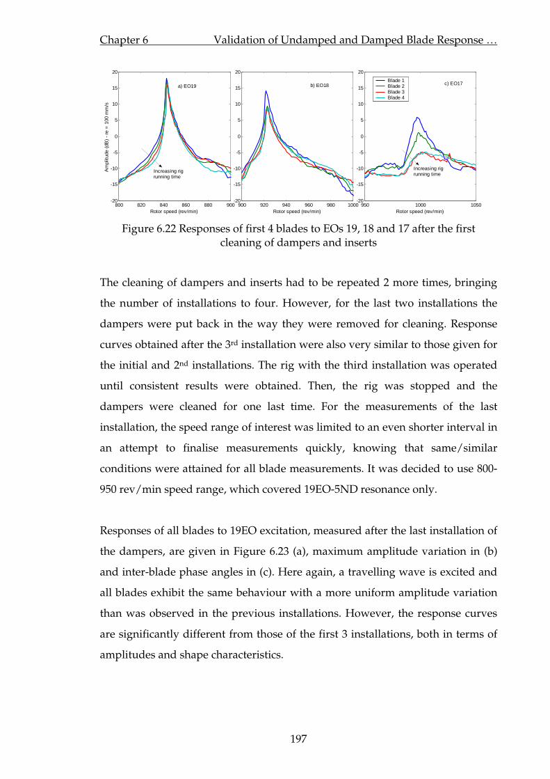
Chapter 6 Validation of Undamped and Damped Blade Response …
197
800 820 840 860 880 900-20
-15
-10
-5
0
5
10
15
20
Rotor speed (rev/min)
Am
plitu
de (
dB)
- re
= 1
00 m
m/s
900 920 940 960 980 1000-20
-15
-10
-5
0
5
10
15
20
Rotor speed (rev/min)950 1000 1050
-20
-15
-10
-5
0
5
10
15
20
Rotor speed (rev/min)
Blade 1Blade 2Blade 3Blade 4
a) EO19 b) EO18 c) EO17
Increasing rig running time
Increasing rig running time
Figure 6.22 Responses of first 4 blades to EOs 19, 18 and 17 after the first cleaning of dampers and inserts
The cleaning of dampers and inserts had to be repeated 2 more times, bringing
the number of installations to four. However, for the last two installations the
dampers were put back in the way they were removed for cleaning. Response
curves obtained after the 3rd installation were also very similar to those given for
the initial and 2nd installations. The rig with the third installation was operated
until consistent results were obtained. Then, the rig was stopped and the
dampers were cleaned for one last time. For the measurements of the last
installation, the speed range of interest was limited to an even shorter interval in
an attempt to finalise measurements quickly, knowing that same/similar
conditions were attained for all blade measurements. It was decided to use 800-
950 rev/min speed range, which covered 19EO-5ND resonance only.
Responses of all blades to 19EO excitation, measured after the last installation of
the dampers, are given in Figure 6.23 (a), maximum amplitude variation in (b)
and inter-blade phase angles in (c). Here again, a travelling wave is excited and
all blades exhibit the same behaviour with a more uniform amplitude variation
than was observed in the previous installations. However, the response curves
are significantly different from those of the first 3 installations, both in terms of
amplitudes and shape characteristics.

Chapter 6 Validation of Undamped and Damped Blade Response …
198
260 270 280 290 300-25
-20
-15
-10
-5
0
Am
plitu
de (
dB)
- re
= 1
00 m
m/s
Frequency (Hz)0 5 10 15 20 25
-200
-150
-100
-50
0
50
100
150
200
Blade #
Inte
r-bl
ade
phas
e an
gel (
deg)
From (a)Perfect travelling wave
0 5 10 15 20 250
0.1
0.2
0.3
0.4
0.5
0.6
0.7
0.8
0.9
Am
plitu
de (
V)
- 1
V =
100
mm
/s
Blade #
Max. amp. variation, from(a)(a) - 5ND mode excited by 19EO
(b) (c)
Figure 6.23 (a) 19EO response of all blades after 4th and last installation of dampers; (b) maximum amplitude, and (c) inter-blade phase angle variation.
6.6.3.5 Comparison of measurements of different installations
In order to reveal the extent of the departure in dynamic behaviour of the
dampers in the last installation from that of the previous three, the responses of
blade 1 to 19EO excitations for all installations are overlaid and given in Figure
6.24 (a). Also shown in this figure is the corresponding undamped response
curve for the same blade. Despite the good correlation of the first three
installations, the fourth one presents a substantial shift in the resonance
frequency with much reduced amplitudes. Bearing in mind that the normal load
(i.e. the centrifugal force acting on the dampers) and excitation forces were kept
the same in all installations, the deviation can probably be attributed to a
substantial change in the surface characteristics of the dampers. This might have
been incurred during the process of cleaning as well as a result of the bedding
period, so as to increase the friction damping and contact stiffness, thus resulting
in lower amplitudes and a higher resonance frequency. However, to the best
knowledge of the author, no particular action during the cleaning was taken to
yield such a drastic change. Close inspection of the dampers after the tests with
the final installation, once again, revealed the formation of brown patches on the
damper surfaces resulting from the accumulation of debris. When compared
with the undamped response curve, the first three installations yielded the same
natural frequency. This was because the vibration amplitudes were higher in
these installations so that the dampers were further away from the stuck

Chapter 6 Validation of Undamped and Damped Blade Response …
199
condition. Thus, although the damping in the system was increased, no
additional stiffness was provided by the dampers. However, in the case of the 4th
installation, the dampers were much closer to the stuck condition, and as a result
they increased the stiffness of the system as well as the damping.
Short samples of time histories of the first 6 blades are given in Figure 6.24 (b)
and (c), and these were measured after the first and last installations of the
dampers, respectively. The lower frequency oscillations are due to laser beam-
rotation axis misalignment. The fact that each blade received the magnetic force
at a slightly later time was perfectly manifested by the given time histories,
which exhibited larger amplitudes at magnet passing times. Although the blisk
as whole was excited at all times, enough damping was produced that the
vibrations on a particular blade were much reduced (in some cases completely
damped out) by the next magnet passing time. However, in the close proximity
of the shown resonance peak, the first three installations showed no clear sign of
decay in vibration amplitudes.
255 260 265 270 275 280 285 290-20
-10
0
10
20
30
40
Frequenc (Hz)
Am
plitu
de (
dB)
- re
= 1
00 m
m/s
Installation # 1 " # 2 " # 3 " # 4Undamped
Bla
de #
0 0.02 0.04 0.06 0.08 0.1 0.12
Bla
de #
Trigger signal Time histories
1
2
3
4
5
6
6
5
4 3
2
1
(a) (b)
(c) Ω=884 rev/min
Figure 6.24 (a) Response of blade 1 to 19EO excitation for all installations, and time histories @ 884 rev min for (b) installation 1 and (c) installation 4.

Chapter 6 Validation of Undamped and Damped Blade Response …
200
6.6.3.6 Variation of response with amplitude of excitation force
Additional measurements were performed for the last installation in the 700-800
rev/min speed range, covering the 20EO-4ND mode resonance. The responses
of the first 5 blades in the speed range (to check the consistency) and the
circumferential ODS at the mentioned resonance were measured. Corresponding
results of the latter are given in Figure 6.25 (a) and (b). The inter-blade phase
angles at the identified resonance are also given in (c).
235 240 245 250 255 260 265-20
-15
-10
-5
0
5
10
15
20
25
Frequency (Hz)
Am
plitu
de (
dB)
- re
= 1
00 m
m/s
Blades # 1 to 5
2 4 6 8 10 12 14 16 18 20 22 24-200
-150
-100
-50
0
50
100
150
Inte
r-bl
ade
phas
e an
gel (
deg)
Blade #
From ODS @ 20EO-4ND resonance
2 4 6 8 10 12 14 16 18 20 22 240
2
4
6
8
10
12
14
16
18
20
Blade #
from ODS @ 20EO-4ND resonance(a) - 4ND mode excited by 20EO
(b) (c)
Figure 6.25 (a) Response of first 5 blades to EO20 excitation, (b) blade-to-blade amplitude variation, and (c) inter-blade phase angles @ the resonance speed.
The main goal in this last set of measurements was to measure the response of a
particular blade for various magnet-blade gaps, and to observe the changes in
the response characteristics as a result of different excitation levels. Figure 6.26
(a) shows the variation of the peak-to-peak amplitude of the force signal with
rotational speed for 4 different magnet-blade distances. The corresponding
response curves are given in (b). The black curve in (a) reveals significant force
magnitude modulation around the resonance. This is because around resonance
standing-wave vibration (i.e. travelling wave excitation excites a standing wave,
fixed in space) causes a change in the gap between the magnet and the blades
which, with a close clearance as in the black curve in (a), affected the force level
considerably. As the clearance was increased, this effect became negligible.

Chapter 6 Validation of Undamped and Damped Blade Response …
201
It is clearly seen from Figure 6.26 (b) that the damping and apparent natural
frequency increased with a decrease in the magnetic (excitation) force, as the
dampers moved closer to the 'stuck' condition.
235 240 245 250 255 260 265-10
-5
0
5
10
15
20
25
30
Am
plitu
de -
(dB
) -
re 1
00 m
ms
-1/N
Frequency (Hz)
240 250 2600
2
4
6
8
10
12
14
16
Frequency (Hz)
Mag
net
puls
e am
p. -
pea
k-to
-pea
k (N
)
Magnet-blade distance ~= 3 mm " ~= 3.5 mm " ~= 3.75 mm " ~= 4 mm
(a)
(b)
Decreasing excitation force (rotor speed - rev/min) (720 750 780)
Figure 6.26 (a) variation of force signal amplitude with rotational speed, (b) response of blade 1 to EO20 excitation at various blade-magnet distances
6.6.4 Validation of damped forced response predictions
6.6.4.1 Strategy of validation process
Validation of the damped vibration response predictions was carried out by
using a subset of the experimental results as presented in previous section.
Owing to the variability observed in measured response characteristics between
different installations, the predicted results were compared with all installations
whenever the corresponding experimental data were available. These variations
also necessitated that a range of contact parameter values be used in order to
capture the true behaviour at different stages of the test campaign (i.e. different
installations).
Chapter 6 Validation of Undamped and Damped Blade Response …
202
It was observed that the first 3 installations exhibited similar dynamic behaviour
which was different from that of the last installation. In order to help explain this
variation, the predictions were repeated for different contact parameter values.
The results showed that the damped blisk response was insensitive to contact
stiffness variations. On the other hand, the normal load and the coefficient of
friction were found to be significantly affecting the response characteristics.
Since the normal load was known accurately (i.e. centrifugal load acting on
dampers of known masses), the observed variation between the different
installations was likely to be caused by variation in the friction coefficient. The
predictions were carried out first for a friction coefficient of 0.45. This figure, as
mentioned, was measured earlier for the titanium alloy used and was expected
to yield close predictions for the results of the first 3 installations. The
preliminary predictions showed that varying the coefficient of friction from 0.45
to 0.6 allowed the variability observed in the vibration response measured to be
covered. Therefore, additional predictions were performed by using a coefficient
of friction of 0.6 to explain the results measured for the last installation. In
following sub-sections, first the predictions obtained by using µ =0.45 (i.e.
simulating the first 3 installations) are presented and then they are repeated for
µ =0.6 (i.e. simulating the measurements of the last installation). In both cases,
the measurement results obtained from all installations are included in the plots
for the sake of comparison.
6.6.4.2 Predictions of the first 3 installations – 19EO excitation
As presented in the previous section, the main effort was directed to the
measurement of the 19EO-5ND resonance though 17, 18, and, in some cases, 20
EO excitations were also considered. The 19EO response of blade 1 for all 4
installations is compared to the corresponding predictions ( µ =0.45) in Figure
6.27. The predictions were repeated for two cases where mono- and multi-
harmonic forcing was considered. The results of both analyses are shown in the
figure. In the case of multi-harmonic force, 5 harmonics (17 to 21) were

Chapter 6 Validation of Undamped and Damped Blade Response …
203
considered. Additionally, although the normal load was taken as constant
(normal load at the rotor speed exciting the 19EO-5ND resonance was applied
for the frequency range used), in the mono-harmonic force case, its variation
with rotational speed was taken into consideration for the multi-harmonic case.
It was shown during the presentation of undamped results in this chapter
(Section 6.6.2) that, in the close proximity of resonances corresponding to lower
ND 1F family of modes, the response curves of the tuned and mistuned system
were practically the same (see Figure 6.18). Therefore, for the computations of
non-linear response of 17-20 EO excitations, the mistuning in the blisk was not
taken into account. For the case of 17EO excitation, the response curves were
compared for a speed range in which the undamped-tuned and -mistuned blisk
responses were reasonably close, see Figure 6.18 (b).
260 270 280 290 300 310 320 330-30
-20
-10
0
10
20
30
40
50
Frequency (Hz)
Am
plitu
de (
dB)
- re
100
mm
/s
Exp. - 1st InstallationExp. - 2nd installationExp. - 3rd installationExp. - 4th installationFORSE - Constant normal load, mono-harmonic forceFORSE - Variable normal load, multi-harmonic forceExp. - Undamped
Figure 6.27 Comparison of measured and computed damped Blisk-1 response on blade # 1 to 19EO excitation; µ =0.45
It is clearly seen from the figure that the predictions correlate much better with
the first 3 installations than the last one. The apparent natural frequency of the
damped system obtained from the first 3 installations and the predictions was
almost the same as that of the undamped system. (Note that the undamped
curve given in the figure was obtained by amplitude-scaling of the original

Chapter 6 Validation of Undamped and Damped Blade Response …
204
curve, which was measured in the presence of a much smaller input force). This
meant that the dampers did not increase the stiffness of the blisk. As the
vibration amplitudes were sufficiently large, the dampers slid on the blade insert
faces freely. Therefore, their contribution to the system stiffness was minimal.
The consideration of variable normal load and of, especially, multi-harmonic
vibrations, produced better predictions, particularly at positions away from the
main resonance. The solid black curve in Figure 6.27 follows the measurements
reasonably, both qualitatively and quantitatively. In order to verify the
assumption that the blisk behaved as tuned for the results presented, the
predictions were repeated by taking the mistuning in the blisk into account.
However, no significant difference was observed between the tuned and
mistuned cases.
Despite the mentioned similarities between the measurements of the first 3
installations and the predictions given in Figure 6.27, the resonance amplitudes
predicted were much higher. In fact, close inspection of the time data measured
at around the resonance revealed similar behaviour to the undamped case,
where the large amplitudes led to truncation of the vibration signal. Likewise,
the true resonance peak amplitude could not be measured as the speed steps
were not sufficiently fine. At this stage it is necessary to note that, when no
stiffness contribution is introduced, the damping introduced through friction
does not limit the vibration amplitudes but lowers them by a finite amount. That
is to say, when an undamped system is integrated with friction dampers which
provide damping only, the resonance peak amplitudes will still be infinite. In
this particular case, the resonance peak amplitude was determined mainly by
the available structural damping, which was very low (η =0.000075).
Nonetheless, the predictions showed that compared with the undamped case, a
70% reduction in the resonance peak amplitude was achieved by the dampers.

Chapter 6 Validation of Undamped and Damped Blade Response …
205
6.6.4.3 Predictions of the first 3 installations – 17-18EO excitations
Response curves measured for 18 and 17 EO excitations were also correlated
with predictions, as shown in Figure 6.28. The speed range used for the 4th
installation was smaller as it was intended to cover the 19EO-5ND resonance
only. Although not completely to be compared with the other curves, the
extracted response of 18EO excitation for this case was given as an indication of
the departure in the behaviour of different installations. Only the predictions
with variable normal load and multi-harmonic force are shown. Most of the
observations noted for the 19EO excitation curves given above apply to those of
the 18EO case given in Figure 6.28 (a). Despite the unavailability of the complete
response curve, the behaviour of the last installation is, again, considerably
different from the others. As for the 17EO excitation response, a different trend
was observed between the predictions and the measurements. Here, the
dampers were predicted to be working more effectively thanks to the higher
normal load. In fact, the increase in the normal load (i.e. due to increasing
rotation speed) was around 10%, which demonstrated that the performance of
the dampers was very sensitive to the normal load. Measurement data from the
last installation was not available and therefore is not given. For all other
installations, the response curves obtained for blade 1 were similar and
somehow dissimilar to the predicted one. Particularly near the resonance peak,
the amplitudes as well as the apparent natural frequency were observed to be
different. Recalling the variability encountered in the measurements of the 1st
installation, the response of the minimum responding blade (blade # 18) is also
given in Figure 6.28 (b) to indicate the range of variation. The amplitude
response of this blade correlated well with that of the predicted curve but the
frequency axis did not. As the actual dampers were working more effectively at
speeds near the 17EO-7ND resonance (and in all installations) and closer to the
stuck condition, their contribution to the stiffness of the system was now
notable. This led to an increase in the natural frequency of the mode in question
which was not predicted as accurately as the amplitudes were.

Chapter 6 Validation of Undamped and Damped Blade Response …
206
230 240 250 260 270 280 290-35
-30
-25
-20
-15
-10
-5
0
5
Frequency (Hz)
Exp. - 1st installation, blade #1Exp. - 1st installation, blade #18Exp. - 2nd installation, blade #1Exp. - 3rd installation, blade #1FORSE - Var. norm. load, multi-harm. vibs.
240 250 260 270 280 290 300 310
-40
-30
-20
-10
0
10
20
30
Frequency (Hz)
Am
plitu
de (
dB)
- re
100
mm
/s
Exp. - 1st InstallationExp. - 2nd installationExp. - 3rd installationExp. - 4th installationFORSE - Variable normal load, multi-harmonic vibrations.
(a) (b)
Figure 6.28 Comparison of measured and computed damped Blisk-1 response on blade # 1 to (a) 18, and (b) 17 EO excitations; µ =0.45.
6.6.4.4 Predictions of the last installation – 18-19 EO excitations
The predictions were repeated by using a friction coefficient of 0.6. In this case it
was expected to simulate the measurements of the last installation. The vibration
response data for the 17EO-7ND resonance was not available for the last
installation and only the 18 and 19 EO excitation responses were compared. The
comparisons obtained are given in Figure 6.29.
260 270 280 290 300 310 320 330-25
-20
-15
-10
-5
0
5
10
15
20
Frequency (Hz)
Exp.1st inst., blade #1Exp.2nd inst., blade 1Exp. 3rd inst., blade #1Exp. 4th inst., blade #1 FORSE - Variable No,
multi-harmonic vibs, µ=0.6
240 250 260 270 280 290 300 310
-30
-25
-20
-15
-10
-5
0
5
10
15
20
Frequency (Hz)
Am
plitu
de (
dB)
- re
100
mm
/s
(a) (b)
Figure 6.29 Comparison of measured and computed damped Blisk-1 response on blade # 1 to (a) 18, and (b) 19 EO excitations; µ =0.6.

Chapter 6 Validation of Undamped and Damped Blade Response …
207
The predictions obtained in this case were clearly better correlated with the
measurements of the last installation, as expected. It is seen from the figure that
the increase in the coefficient of friction from 0.45 to 0.6 resulted in a significant
reduction in response amplitudes, covering the range of amplitude variation
observed at various stages of the measurements. This finding strengthens the
explanation that the mentioned response variation between the first 3
installations and the last was due to variation of coefficient of friction. Despite
the incompleteness of the data, Figure 6.29 (a) shows very good agreement
between the measurements of the last installation and the predictions. Although
the amplitudes are not predicted as accurately in Figure 6.29 (b), a reasonable
qualitative agreement is evident. However, in both Figure 6.29 (a) and (b), the
apparent natural frequency is under predicted. Since the predictions for the
undamped blisk for this resonance frequency were demonstrated to be closer,
the discrepancy here is probably due to the modelling of the under-platform
dampers.
At this stage it is worth mentioning that although the predictions are given for
two extreme values of coefficient of friction, the actual values of this parameter
in reality were probably changing even within the same measurement session.
By giving predictions for different values of coefficient of friction, it was aimed
to show that provided that the correct values of this parameter were available at
corresponding stages of the measurements, reasonable predictions could be
obtained. The evidence presented in this section demonstrated that the
prediction tool was capable of providing reliable estimates for a blisk integrated
with under-platform friction dampers once the correct input parameters were
supplied.
6.7 Summary
In this chapter, the predictions of the damped and undamped vibration response
of Blisk-1 have been validated against the measurements. The following steps

Chapter 6 Validation of Undamped and Damped Blade Response …
208
have been taken in achieving this: (i) translation of frequency mistuning to
physical mistuning and its validation, (ii) evaluation of EO excitation errors and
their effects, (iii) analysis of mistuning errors, (iv) validation of the undamped
response predictions and the test setup (rig + Blisk-1), (v) identification of
damper operation regions, and finally (vi) the validation of damped response
predictions.
First, the principles and capabilities of the non-linear response prediction tool
used were introduced. Then, the frequency mistuning identified in Chapter 4
was translated into physical mistuning. It was found that the closest results were
obtained when mistuning was represented by the nodes at the blade tips as
opposed to platform levels. For the family of modes of interest (1F), the nodes at
a given locality underwent a similar pattern of deflection that the location of
mistuning nodes was a more important factor than their number.
It was observed that the amplitude of the magnetic force experienced by each
blade was slightly different, thus introducing EO excitation errors. This was
expected to have been caused by a combination of possible factors including: (i)
a bent shaft, (ii) swash errors, and (iii) different blade tip masses etc. The effect of
excitation error was studied using the FE model of Blisk-1. The predictions on
the mistuned Blisk-1 showed that the variability of the magnetic force observed
in the experiments had negligible effect on the forced response. Using the same
model and by applying 10000 randomly generated excitation patterns, it was
shown that the variation caused in the forced response was less than the
variability in the force input. It was also shown that errors in the applied EO
excitation (i.e. non-uniform amplitudes) would cause several ND modes of a
tuned system to be excited. However, the amplitudes of additional resonance
peaks were found to be very small compared with those caused by physical
mistuning. Additionally, the errors in the mistuning pattern identified were also
studied using the lumped parameter model introduced in Chapter 4. This
pattern was found to be robust for the variation envisaged.

Chapter 6 Validation of Undamped and Damped Blade Response …
209
The undamped Blisk-1 response predictions were compared with the
measurements and good correlation was observed. Both, z-mod plots and
individual blade response levels were shown to be closely predicted. The
alignment of the laser beam with the rotation axis was notably worse for Blisk-1
measurements (possibly because of a bent shaft). As a result, considerable
discrepancies were observed around resonances excited at high rotor speeds.
However, this effect was shown to have receded for the same resonances when
excited at low rotor speeds. Although the comparison of all blade response
curves was not as convincing as those of Blisk-2 (see Chapter 5), they were
sufficiently close to validate the mistuning pattern identified and its modelling.
In the final part of the chapter, measurements taken on the damped Blisk-1 were
reported, and then a subset of these results were compared with the predictions.
Preliminary investigations showed that the steel dampers were too heavy for
most of the speed range and the titanium dampers did not operate adequately at
high speeds. Therefore, the main effort was directed at the testing of the titanium
dampers at low speeds where 17-20 EOs were exciting 7-4ND modes,
respectively. It was observed that during the operation of the rig, the
characteristics of the contact interfaces changed with time. This was due to the
accumulation of metal debris knocked off the rubbing faces. As a result, the
dampers and the blade inserts had to be cleaned and reinstalled 4 times. The
results obtained for the first three installations were consistent and significantly
dissimilar to those of the final installation. Nonetheless, each set of
measurements was consistent in itself which proved the essential reliability of
the measurement process itself.
Preliminary predictions with various values of contact stiffness, coefficient of
friction and normal load showed that the blisk response was not sensitive to
contact stiffness but that it varied significantly with latter two parameters. As the
normal load was known fairly accurately, the predictions were repeated for two

Chapter 6 Validation of Undamped and Damped Blade Response …
210
extreme values of the coefficient of friction in an attempt to account for the
variability observed during the measurements. The first value (0.45) was
expected to simulate the real situation in the first three installations where the
dampers were known to have slid freely at the contact interfaces. On the other
hand, the second value (0.6) was used to predict the measurements of the last
installation in which the dampers were closer to the stuck condition. Both cases
revealed acceptably close correlation with the measured results they were
expected to simulate.
Chapter 7 Conclusions and Future Work
211
CHAPTER 7
CONCLUSIONS and FUTURE WORK
7.1 Summary and Conclusions
The main goals of the presented study, as stated in Chapter 1, were to provide
reliable and accurate measure of vibration data obtained under well-controlled
and realistic conditions so that the forced response predictions of mistuned and
friction damped blisks could be validated. An overview and conclusions drawn
from the work performed towards the fulfilment of these goals are given below.
However, it is appropriate to start with conclusions concerning the devised
measurement technique and test setup, which were also set as major objectives
of this work as means of achieving the abovementioned application aims.
7.1.1 Measurement technique and test rig
The devised self-tracking measurement technique worked successfully and
proved to be an effective and reliable way of measuring response on rotating
components such as bladed disks. The fact that this technique, as indeed do all
other LDV measurement techniques, relied on proper alignment of the laser
beam with the axis of rotation, led some of the EO excitation responses to be
contaminated by the cross-talk errors. For the simpler Blisk-2, these errors have
been minimised and confined to lower EO excitations (which were excluded
from the measurements) through elaborate alignment measures. However, the
effects of misalignment on Blisk-1 measurements have been somewhat more
dominant, probably due to a bent drive shaft, and could not be improved
through the same alignment measures. The measurement rig operated well
under vacuum and throughout the rotating tests without any major breakdown.
Chapter 7 Conclusions and Future Work
212
The use of mechanical indexing enabled all blades to be measured sequentially
and quickly without shutting the rig down. Through repeated measurements
under similar conditions, it was demonstrated that the designed rig was capable
of producing reliable and consistent data, which was essential since they were to
be used for validation purposes.
7.1.2 Mistuning analysis
One of the main objectives of this study was to validate the models used to make
forced vibration response analysis by comparing predictions of mistuned bladed
disk vibration through accurate and well-controlled measurements (i.e.
measurements reflecting the response due to phenomena of interest only). This
was achieved via a reasonably well tuned integral bladed disk testpiece
operating in a vacuum and under rotation, as well as at rest and in the presence
of air. An extensive test design phase was undertaken by using an updated FE
model of the blisk, which was successfully executed in the way it was planned.
This enabled a very efficient test campaign, both in terms of short measurement
times and in the acquisition of useful data. Through the measurements at rest
with several mistuning patterns, it has been demonstrated that the calculation
tool successfully predicted measured circumferential ODSs, as well as natural
frequencies and the splits in double modes. Following this, the rotating
measurements were carried out for three configurations on Blisk-2:
(i) Tuned case: The comparison of measured and predicted interference
diagrams demonstrated excellent agreement. Individual blade responses
were also well predicted though some variations were evident, probably
due to the sensitivity of this tuned case to minor deviations in the test
conditions and excitation errors. It has been demonstrated by way of
rotating ODS measurements that travelling waves were excited in the
blisk, with all blades experiencing the same level of vibration. This level,
again, was predicted reasonably in simulations.
Chapter 7 Conclusions and Future Work
213
(ii) Regular mistuning case, ( )8Sin θ⋅ . This case was designed to display
considerable modal overlap and reasonably complicated mode shapes so
as to form a challenging case for predictions. The good correlation of
measured and predicted natural frequencies (Table 5.1) demonstrated that
the mistuning had been properly modelled. It was shown during the test
design phase that the interference diagram exhibited a formation of
complex resonance groups, which was backed up generously by the
measurements, Figure 5.13. In this case, the modes excited at each
resonance on the interference diagram were accounted for through their
harmonic content, Figure 4.25. This was confirmed by the Fourier analysis
performed on the measured ODSs. A mistuning pattern of this kind was
expected to produce 3 different blade responses for a given EO excitation,
which was gratifyingly proved by the measured response curves for 6EO
excitation, Figures 5.14-15. Individual blade response curve
measurements (Figure 5.15) and blade-to-blade amplitude variations
(Figure 5.17) have been well predicted not only qualitatively but also
quantitatively.
(iii) Random mistuning case. The interference diagram predicted for this case
was rather complicated but compared very well with the measurements,
Figure 5.18. Similarly, modes corresponding to predicted resonances were
identified (Figure 4.27) and confirmed by the measured ODSs. Individual
blade response curves have been measured for a limited speed range for
10EO excitation. Comparisons (Figure 5.19) demonstrated that the
predictions were good not only around the resonance frequencies but also
away from them, thus validating both the predictions and also the
measurement technique. Comparison of measured and calculated ODSs
(Figure 5.23) showed that the blade response amplitudes, as well as the
pattern of variation were, well predicted.
Additional mistuning analyses were conducted on Blisk-1. Non-negligible
inherent mistuning in this testpiece, which could not be removed via tuning,

Chapter 7 Conclusions and Future Work
214
was identified experimentally in terms of scatter of 1F natural frequencies of
isolated sectors, Figure 4.18. This frequency mistuning was later translated into
physical mistuning for forced response analyses. It was demonstrated by mode
shape and natural frequency comparisons that the updated blisk model
represented the real blisk accurately, Figure 4.20. Despite errors in mistuning
identification, and to an extent in its representation, relatively complex response
curves measured in a narrow frequency band were reasonably well predicted
(Figure 6.12), with acceptable accuracy.
In forced response predictions, the effect of rotational speed was accounted for
by calculating the mode shapes and frequencies at the mid-speed value of the
range of interest, and then by rearranging the frequency axis of the forced
response curves according to rotational speed-frequency shift relation, Figure
5.5. The good level of agreement verified that the implemented approach was
appropriate. Also, the close agreement between the measured and predicted
response levels confirmed that the forcing input was processed accurately.
Since the blisks used in the analyses were very lightly damped, the resonances
were very sharp and produced very large vibration amplitudes when excited. As
a result, in all abovementioned cases the true resonance amplitudes could not be
captured accurately due to insufficient sweep rates. Also, the frequencies
corresponding to lower modes were lower in measurements due to flexible disk
clamping in measurements as opposed to the rigid fixing assumed in the FE
models. However, in both cases the problems were related to the test setup
rather than to the prediction tool. In the light of evidence presented in this study,
the forced response blade vibration prediction tool has been demonstrated to be
predicting the tuned and mistuned vibration response accurately, and has thus
been successfully validated. Most of the experimental studies reported in the
reviewed literature, which were also aimed at validation of numerical codes,
dealt with stationary components. The fact that very good agreement between
the measurements and the predictions was obtained under rotating conditions,
Chapter 7 Conclusions and Future Work
215
simulating a more realistic situation, stands out as an important achievement of
this study.
7.1.3 Friction damping analysis
The second goal sought in this study was to validate the predictions of bladed
disk forced response when under-platform friction dampers were integrated in
the testpiece. This was achieved through measurements performed on Blisk-1.
Two sets of dampers, one made of steel and the other made of titanium, were
tested. Tests carried out on the steel dampers were not effective as they proved
to be too heavy to operate as desired, Figure 6.16. These dampers were found to
be locking up at relatively low rotation speeds, thus raising the natural
frequencies of the bladed disk assembly through substantial stiffness increases.
As a result, only the dampers made of titanium were used in the measurements
reported here. Some difficulties were encountered in making these dampers
function satisfactorily, too, particularly at high rotation speeds where reasonably
well tuned low ND modes were excited. Testing of these modes was particularly
important as the higher ND ones (7ND and higher) were significantly mistuned.
Since the mistuning was not known accurately, the predictions involving these
modes would have been less certain. As a result, a speed range covering
resonances corresponding to the 1F family of blisk modes excited by 17, 18, 19,
20, and 21 EOs (i.e. 7, 6, 5, 4, and 3ND modes respectively) was covered. The
main effort was directed towards 19 and 20 EOs so that reasonably tuned 4 and 5
ND modes were excited.
It was observed that the dynamic characteristics of the dampers changed as the
rig operated, Figure 6.20. The titanium dampers were in contact with steel
surfaces. As the dampers worked effectively, they removed metal from the steel
surfaces they worked against. In time this removed metal accumulated in
between the contact surfaces, gradually leading to rougher surfaces and higher
damping, or, in some cases, even to jamming of the dampers, Figure 6.21. As a

Chapter 7 Conclusions and Future Work
216
result, it was necessary to clean the accumulated debris from the contact surfaces
several times. Overall, the dampers were taken out and reinstalled 4 times over
50 hours of operating time and the measurements repeated after each
installation. It was observed that the first 3 installations of the dampers yielded
similar response characteristics in terms of resonance frequencies and peak
amplitudes. However, the 4th one, in which the damping and stiffness
contributions of the dampers were considerably higher, differed significantly
from the first three, Figure 6.24. Although the resonance peak amplitudes
measured in the first installation differed somehow from blade to blade, all the
blade responses, in general, exhibited considerable consistency in each
installation. This proved that the rig with friction damped blisks produced
reliable and repeatable vibration response data.
The modelling of Blisk-1 with under-platform friction dampers was achieved by
considering a single sector and making use of cyclic symmetry. Since the
measurements were concentrated on the mainly tuned blisk modes, the
mistuning in the blisk was assumed negligible and not considered. This
assumption was verified by comparing the undamped-tuned and –mistuned
response predictions (Figure 6.18) for these modes as well as the damped-tuned
and -mistuned ones. The coefficient of friction used was taken from earlier
measurements performed for the titanium alloy employed. However, the contact
stiffness was calculated by FE analysis. Owing to the uncertainties regarding the
contact parameters (i.e. contact stiffness and friction coefficient), some
preliminary predictions were performed to find out the sensitivity of the system
response to these parameters. The contact stiffness was found to have a less
impact than the friction coefficient which, together with the normal load, was
demonstrated to have played a greater role in determination of the response
characteristics. Since the normal load was accurately known, the friction
coefficient was varied to account for the variability observed during the
measurements. By systematically changing the coefficient of friction from 0.45 to
0.6 the variation obtained between different installations of the dampers could

Chapter 7 Conclusions and Future Work
217
be accounted for. Therefore, the predictions were performed and presented for
these two extreme values of the friction coefficient.
It was observed that the damped response predictions for a friction coefficient of
0.45 correlated much better with the results of the first 3 installations than the
last one (Figure 6.27), as expected. The agreement was further improved by
consideration of multiple harmonic vibrations and variable normal load.
However, the predicted and measured peak resonance amplitudes were
considerably different for some of the resonances measured (19EO-5ND and
18EO-6ND). Since the dampers in the first 3 installations slid freely along the
blade insert faces, they did not cause any stiffness increase in the blisk. The
comparison of the damped and undamped measurements showed little change
in apparent natural frequency. In this case, although the amplitudes were
reduced by a finite amount due to friction damping, the resonance peak
amplitudes were mainly determined by the available structural damping, which
was very low. As a result, large vibration amplitudes were created but could not
be measured accurately due to insufficient sweep rate. However, for the 17EO-
7ND resonance, which was excited at a relatively higher rotation speed, better
estimates were obtained in terms of resonance peak amplitudes. In this case, the
normal load was slightly higher due to higher rotation speeds and, the dampers
were closer to the stuck condition. This meant that the damping produced was
more effective and kept the resonance peak amplitude reasonably low so that it
could be measured accurately, Figure 6.28.
The damped response predictions were repeated for an upper extreme value of
friction coefficient of 0.6. This was done to help explain the results obtained in
the last installation of the dampers. The limited range of data available allowed
only 18 and 19 EO excitation responses to be compared with the predictions.
Clearly, better estimates were obtained for the last installation of the dampers,
Figure 6.29. The 18EO excitation response was found to be better predicted than
the 19EO excitation. This was probably due to the fact that the contact conditions
Chapter 7 Conclusions and Future Work
218
were changing even within the same measurement session, at different rotation
speeds. However, the same parameters were applied in a given prediction
session. Some discrepancy was observed between predicted and measured
resonance frequencies as well. As those of the undamped assembly were
demonstrated to have correlated better, the disagreement with the damped
assembly was probably due to the modelling of the friction dampers.
Nonetheless, given the complicated nature of the task and based on the evidence
presented, the prediction tool was demonstrated to be capable of supplying
reliable estimates for blisks integrated with under-platform friction dampers
provided that the correct input parameters were made available.
Most of the studies reported in the reviewed literature dealt with the problem of
under-platform friction damping on simple test setups such as the ones
comprising two blades and a damper in between, at rest. Even when a full
assembly has been tested, the testing was performed on bladed disks having
separately made blades. Thus, the effect of under-platform friction dampers
alone could not be analysed as the contact at the blade roots was also non-linear
and contributed to the response. To the best knowledge of the author, testing at
the scale presented here, reflecting the isolated effects of friction damping, with
such consistency, and under such realistic conditions has not been reported
before. The fact that successful analyses have been performed with acceptable
accuracy fulfils one of the main objectives of the presented work.
7.1.4 Blisk tuning and excitation errors
The attempts made at improving the symmetry of a blisk by tuning its 1F blade-
alone frequencies failed to produce a reasonably well-tuned test piece. In this
study the tuning was performed to obtain a better reference state with which the
effectiveness of the theory could be assessed. However, in practice this is done to
avoid the adverse affects (i.e. mode localisation and thus amplitude
magnification) of the mistuning. It is done because the design is generally based

Chapter 7 Conclusions and Future Work
219
on the amplitudes corresponding to the tuned case. The finding here has been
that, when performed through appropriate parameters, the 1F blade-alone
natural frequency tuning can be successful. However, in general, an effective
tuning can only be achieved if multiple frequencies of the isolated components
(i.e. blades) are matched; a very difficult, long and expensive process in practice.
However, it is known that only certain mistuning patterns are likely to cause
critical vibration amplitudes. Thus, if the pattern of variation is known (which
requires multiple frequencies of each of the blades to be measured), using the
validated prediction tool, the consequences of present mistuning can be
predicted and the combinations likely to cause problems can be eliminated.
Therefore, it is argued that for more efficient use of resources, it is advantageous
to concentrate on identification of mistuning pattern first, rather than trying to
correct it no matter what it is.
The effects of EO excitation errors (i.e. all blades experiencing different force
amplitudes but perfect phase shifts) were investigated through Blisk-1 FE model.
The analyses showed that a kth EO excitation excited many of the non- kth ND
modes of a tuned blisk (Figure 6.7), depending on the pattern of amplitude
variation. However, the amplitudes of these resonances were very small
compared to those caused by the physical mistuning. The deviation of maximum
response (i.e. at the EO-ND resonance) was analysed by using a large number of
cases and it was found that the variation of the maximum amplitude (<3%) was
less than the excitation error (±5%). Thus, it is concluded that the excitation
errors, unlike physical mistuning, are highly unlikely to cause excessive
vibration amplitudes, and, depending on the application, can be neglected.
7.2 Recommendations for future work
The measurement technique devised in this study allowed blade tip responses to
be measured using the self-tracking LDV measurement technique and
circumferential ODSs through the circular scanning LDV under rotation.

Chapter 7 Conclusions and Future Work
220
However, often it is of interest to be able to measure the radial ODSs, say along
the blades, or area scan measurements across the whole bladed disk under
rotation. Although the latter can readily be performed on the current
configuration, a precise measure of rotation speed is needed and a way of data
processing needs to be developed. The former, on the other hand, cannot be
performed with the current setup. However, with the aid of a dedicated research
activity, either through additional optical mechanisms or new scanning
techniques utilising the positioning mirrors of the laser device, the rig can still be
employed in the pursuit of the technology.
Rotational speed dependency of the excitation in the rig meant that the
minimum frequency resolution was limited by the precision of the motor
controller. As a result, it has not been possible to perform detailed
measurements around the sharp resonances which were often encountered. The
use of electromagnets, instead of permanent ones used in this study, can
eliminate this problem as any frequency can be input to the system. The trials
conducted with available a/c magnets have been fruitless as it was not possible
to exert enough force at safe stand offs. New research into development of a
more powerful and compact a/c magnet, and its control to produce desired
force input signals could improve the quality of measurements.
It is known that modes from different families of a bladed disk may interact
strongly at regions where they get close. This phenomenon is called “curve
veering” (from the fact that the families of modes approach and divert from each
other as they never cross) and is particularly important under rotation when a
family of bending modes is reasonably close to but lower than a family of torsion
modes. What happens under rotation is that the bending natural frequencies
increase more with rotational speed than the torsional ones. As a result, these
two families can be brought sufficiently close at veering regions that their modes
interact, producing unexpectedly high amplitudes. The fact that the designed
test rig runs under rotation can be employed in pursuit of this problem by

Chapter 7 Conclusions and Future Work
221
designing a suitable new test piece. Additionally, as it is stands at the moment,
the rig and the test pieces used in the analyses can be employed in quest of
experimental investigation of the effects of other mistuning problems such as
mode localisation, amplitude magnification and intentional mistuning.
The combination of different metals (i.e. titanium dampers operating on steel
surfaces) for friction damping investigation created unexpected problems which
made the characterisation and predictions of the non-linear system difficult.
Now that a rig to carry out this type of experiments is available, by making both,
dampers and blade inserts from the same material, a better understanding of the
problem may be obtained.
References
222
REFERENCES
[1] Ewins, D. J.
Structural dynamics characteristics of bladed disks AGARD Manual on aeroelasticity in axial-flow turbomachines, Vol. 2, 1988
[2] Ewins, D.J.
The effect of blade mistuning on vibration response – a survey IFToMM 4th Int. Conf. on Rotordynamics, Prague, Czechoslovakia, 1991
[3] Srinivasan, A. V.
Flutter and Resonant Vibration Characteristics of Engine Blades ASME Journal of Engineering for Gas Turbines and Power, Vol. 119, 1997, p. 742-775.
[4] Slater, J.C., Minkiewicz, G. R., Blair, A. J.
Forced response of bladed disk assemblies – A survey The shock and vibration digest, Vol. 31, No. 1, January 1999, p.17-24
[5] Moyroud F., Fransson T., Jacquet-Richardet G.
A comparison of two finite element reduction techniques for mistuned bladed disks Journal of Engineering for Gas Turbines and Power, Vol. 124, No. 4, p.942-952
[6] Rivas-Guerra, A. J., Mignolet, M. P.
Local/Global effects of mistuning on the forced response of bladed disks Proceedings of ASME TURBO EXPO, 2001-GT-0289.
[7] Judge, J., Pierre, C., Mehmed, O.
Experimental investigation of mode localization and forced response amplitude magnification for a mistuned bladed disk ASME Journal of Engineering for Gas Turbines and Power, Vol. 123, 2001, p. 940-950.
[8] Myhre, M., Moyroud, F., Fransson, T. H.
Numerical investigation of the sensitivity of forced response characteristics of bladed disks to mistuning Proceedings of ASME Turbo Expo 2003, June 16-19, 2003, Atlanta, Georgia, USA
[9] Kenyon, J.A., Griffin, J. H.
Mistuned bladed disk forced response with frequency veering Proceedings of 8th National Turbine Engine HCF conf., 14-16 April 2003, California
[10] Bladh, R., Castanier, M. P., Pierre, C.
Component-mode-based reduced order modeling techniques for mistuned bladed disks – Part I: Theoretical models ASME Journal of Eng. for Gas Turbines and Power, Vol. 123, 2001a, p. 89-99.
[11] Jacquet-Richardet, G., Ferraris, G., Rieutord, P.
Frequencies and modes of rotating flexible blade disk-shaft assemblies: A global cyclic symmetry approach Journal of Sound and Vibration, Vol.191 (5), 1996, p.901-915
[12] Yang, M.-T. Griffin, J. H.
A reduced order model of mistuning using a subset of nominal modes ASME Journal of Engineering for Gas Turbines and Power, Vol. 123, 2001, p. 893-900.

References
223
[13] Feiner, D. M., Griffin, J. H.
A fundamental mode of mistuning for a single family of modes Proceedings of ASME TURBO EXPO, 2002, GT-2002-30425.
[14] Petrov, E. P., Sanliturk, K. Y., Ewins, D.J.
A new method for dynamic analysis of mistuned bladed disks based on the exact relationship between tuned and mistuned systems ASME Journal of Engineering for Gas Turbines and Power, Vol. 124, 2002, p. 586 -597.
[15] Lim, S., Castanier, M. P., Pierre, C.
Reduced order modelling and analysis of bladed disks with large mistuning Proceedings of 8th National Turbine Engine HCF conf., 14-16 April 2003, California [16] Mignolet, M. P., Rivas-Guerra, A. J., LaBorde, B.
Towards a comprehensive and direct prediction strategy of the effects of mistuning on the forced response of forced response of turbomachinery blades Aircraft Engineering and Aerospace Technology, Vol. 71, 1999, No. 5, p. 462-469.
[17] Mignolet, M. P., Lin, C.-C., LaBorde, B. H.
A novel Limit Distribution for the analysis of randomly mistuned bladed disks ASME Journal of Eng. for Gas Turbines and Power, Vol. 123, 2001a, p. 388 -394.
[18] Petrov, E., Ewins, D. J.
Analysis of the worst mistuning patterns in bladed disk assemblies Proceedings of ASME TURBO EXPO, 2001, 2001-GT-0292, Orleans, Louisiana, USA
[19] Rivas-Guerra, A. J., Mignolet, M. P.
Maximum amplification of blade response due to mistuning: localization and mode shapes aspects of worst disks Proc. of ASME TURBO EXPO, 2002, GT-2002-30323, Amsterdam, The Netherlands
[20] Kenyon, J. A., Griffin, J. H., Feiner, D. M.
Maximum bladed disk forced response from distortion of a structural mode Proc. of ASME TURBO EXPO, 2002, GT-2002-30426, Amsterdam, The Netherlands
[21] Xiao, B., Rivas-Guerra, A. J., Mignolet, A. P. Identification of the maximum responding blade in mistuned bladed disks Proceedings of the Turbo Expo 2003, GT-2003-38966, Atlanta, Georgia, USA [22] Castanier, P. M. and Pierre, C.
Consideration on the benefits of intentional blade mistuning for the forced response of turbomachinery rotors
ASME Int. Mech. Eng. Congress and Expo., 1997, AD-Vol. 55, pp.419-425
[23] Kenyon, J.A., Griffin, J. H. Forced response of turbine engine disks and sensitivity to harmonic mistuning Journal of Engineering for Gas Turbines and Power, January 2003, Vol. 125, p.113-120
[24] Choi, B.-K., Lentz, J., Rivas-Guerra, A. J., Mignolet, M. P. Optimisation of intentional mistuning patterns for the reduction of the forced response effects of unintentional mistuning: Formulation and assessment
Journal of Eng. For Gas Turbines and Power, January 2003, Vol. 125, pp.131-140 [25] Mignolet, M.P., Rivas-Guerra, A.J., and Delor, J.P.
Identification of Mistuning Characteristics of Bladed Disks from Free Response Data - Part I Journal of Engineering for Gas Turbines and Power, Vol. 123(2), 2001, pp. 395-403.
References
224
[26] Rivas-Guerra, A.J., Mignolet, M.P., and Delor, J.P.
Identification of Mistuning Characteristics of Bladed Disks from Free Response Data – Part II Journal of Engineering for Gas Turbines and Power, Vol. 123(2), 2001, pp. 404-411.
[27] Judge, J.A., Pierre, C., and Ceccio, S.L.
Mistuning Identification in Bladed Disks Proc. of the Int. Conf. on Structural Dynamics Modelling, 2002, Madeira, Portugal.
[28] Feiner, D.M., and Griffin, J. H.
Mistuning Identification of Bladed Disks Using a Fundamental Mistuning Model – Part I: Theory ASME Paper GT2003-38648, Int. Gas Turbine Institute Turbo Expo, Atlanta, Georgia.
[29] Feiner, D.M., and Griffin, J. H. Mistuning Identification of Bladed Disks Using a Fundamental Mistuning Model – Part II: Application ASME Paper GT2003-38648, Int. Gas Turbine Institute Turbo Expo, Atlanta, Georgia.
[30] A B Stanbridge, K Y Sanliturk & D J Ewins Measurement and Analysis of High-Temperature Friction Damper Properties
4th US International Turbine Engine High Cycle Fatigue (HCF) Conference, 1999 [31] Sextro, W.
The calculation of the forced response of shrouded blades with friction contacts and its experimental verification Proc. Of ASME Turbo Expo, 2000, Munich Germany.
[32] Berruti, T., Goglio, L., Filippi, S., Gola, M. M.
A test rig for frictionally damped bladed segments Proc. Of ASME Turbo Expo, 2000, Munich Germany. [33] Yang B.D., Chu M.L., Menq C.H.
Stick-Slip-Separation analysis and nonlinear stiffness and damping characterization of friction contacts having variable normal load – a . Journal of Sound and Vibration, 210(4), 1998, pp. 461-481.
[34] Yang, B.D., Menq C.H.
Characterization of 3D contact kinematics and prediction of resonant response of structures having 3D friction constraint - b. Journal of Sound and Vibration, 217(5), 1998, pp. 909-925.
[35] K.Y. Sanliturk, D.J. Ewins & A.B. Stanbridge
Underplatform dampers for turbine blades: theoretical modelling, analysis and comparison with experimental data ASME Journal of the Engineering for Gas Turbines and Power, v.123, pp.919-929
[36] Sanliturk K.Y., Ewins D.J.
Modeling two-dimensional friction contact and its application using harmonic balance method J. of Sound and Vibration, 193(2), pp. 511-523.
[37] Petrov, E., Ewins, D. J.
Analytical formulation of friction interface elements for analysis of nonlinear multi-harmonic vibrations of bladed disks
Journal of Turbomachinery, Vol. 125, APRIL 2003, pp. 364-371

References
225
[38] Petrov, E., Ewins, D. J. Generic friction models for time-domain vibration analysis of bladed discs
Proc. ASME Turbo Expo 2003, GT-2003-38475, Atlanta, Georgia. [39] Petrov, E.
A method for use of cyclic symmetry properties in analysis of nonlinear multiharmonic vibrations of bladed disks Proc. ASME Turbo Expo 2003, GT-2003-38475, Atlanta, Georgia.
[40] Petrov, E., Ewins, D. J.
Analysis of forced response for nonlinear vibration of mistuned bladed discs Proceedings of 8th National Turbine Engine HCF conf., 14-16 April 2003, California
[41] Lin, C.-C., Mignolet, M. P.
Effects of damping and damping mistuning on the forced vibration response of bladed disks Journal of Sound and Vibration, 1996, Vol. 193(2), pp.525-543 [42] Griffin, J. H.
A review of friction damping of turbine blade vibration Int. Journal of Turbo and Jet Engines, No. 7, 1990, pp.297-307 [43] Ewins, D. J.
The effects of detuning upon the forced vibration of bladed-disks Journal of Sound and Vibration, 1969, Vol. 9, No. 1, p.65-79 [44] Ewins, D. J.
Vibration characteristic of bladed disc assemblies Journal of Mechanical Engineering Science, Vol. 15, No. 3, 1973, pp.165-186 [45] Ewins, D. J.
An experimental investigation of the forced vibration of bladed discs due to aerodynamics excitation
The winter annual meeting of ASME, New York, December 5-10, 1976
[46] Fabunmi, J. A.
Forced vibrations of a single stage axial compressor rotor Transactions of ASME Journal of Eng. for Power, Vol. 102, April, 1980, p.322-328
[47] Wei, S.-T., Pierre, C. Localization phenomena in mistuned assemblies with cyclic symmetry Part I: Free vibrations ASME J. of Vib. Acoustics, Stress and Reliability in Design, Vol. 110, 1988, p. 429-438.
[48] Wei, S.-T., Pierre, C. Localization phenomena in mistuned assemblies with cyclic symmetry Part II: Forced vibrations ASME J. of Vib. Acoustics, Stress and Reliability in Design, Vol. 110, 1988, p. 439-449.
[49] Kruse, M. J., and Pierre, C. An Experimental Investigation of Vibration Localization in Bladed Disks, Part I: Free Response Proc. 42nd ASME Gas Turbine and Aeroengine Cong., 1997, Orlando, Florida, USA.
[50] Kruse, M. J., and Pierre, C. An Experimental Investigation of Vibration Localization in Bladed Disks, Part II: Forced Response Proc. 42nd ASME Gas Turbine and Aeroengine Cong., 1997, Orlando, Florida, USA.

References
226
[51] Marugabandhu, P. and Griffin J.H.
A Reduced Order Model for Evaluating the Effect of Rotational Speed on the Natural Frequencies and Mode Shapes of Blades, Int. Gas Turbine and Aeroengine Con. and Expo, 2000-GT-611, Munich, Germany
[52] Ottarson, G.S., Castanier, M. P., Pierre, C.
A reduced order modelling technique for mistuned bladed disks Proc. Of the 35th AIAA/ASME/EASCE/AHS/ASC Structures, Structural Dynamics and Materials Con, 1994.
[53] Kruse, M. J., Pierre, C.
Forced-response of mistuned bladed disks using reduced-order modeling. Proc. of the 37th AIAA/ASME Structures, Structural Dynamics and Materials Con, Salt Lake City, Utah, 1996.
[54] Judge, J., Pierre, C., Mehmed, O.
Experimental investigation of mode localisation and forced response amplitude magnification for a mistuned bladed disk
Transactions of ASME, Vol. 123, October 2001, pp.940-950 [55] Jones, K. and Cross, C.
A travelling wave excitation system for bladed disks 43rd AIAA/ASME/EASCE/AHS/ASC Structures, Structural Dynamics and Materials Con, AIAA 2002-1531, 2002, Denver, Colorado.
[56] Judge, A. J., Ceccio, S. L. and Pierre, C.
Travelling wave excitation and optical measurement techniques for non-contacting investigation of bladed disk dynamics
The Shock and Vibration Digest, Vol. 34, No. 3, May 2003, pp.183-190
[57] Kenyon, J. A. and Griffin, J. H.
Experimental demonstration of maximum mistuned bladed disk forced response Proceedings of ASME Turbo Expo, GT2003-38060, 2003, Georgia, USA
[58] Shu, H. T. and Cutts, D. G.
Methods of processing strain response signals from rotating bladed assemblies to extract modal parameters
IMAC [59] Hollkamp, J. J. and Gordon, R. W.
Modal test experience with a jet engine fan model Journal of Sound and Vibration, 2001, Vol. 248, No. 1, pp.151-165 [60] Jaiswal, B. L. and Bhave, S. K.
Experimental evaluation of damping in a bladed disk model Journal of Sound and Vibration, 1994, Vol.177, No. 1, pp.111-120 [61] Berruti, T., Filippi, S. and Gola, M. M.
Friction damping of interlocked vane segments: experimental results Proceedings of ASME Turbo Expo, June 2001, 2001-GT-0432 [62] Hollkamp, J. J. and Gordon, R. W.
An experimental investigation of non-uniform damping in bladed disks AIAA-98-3747, 1998

References
227
[63] Jeffers, T.R., Kielb, J.J., Abhari, R.S.
A Novel Technique for the Measurement of Blade Damping using Piezoelectric Actuators ASME 2000-GT-359, IGTI TURBO EXPO Conference, May 2000, Munich, Germany
[64] Burdekin, M., Cowley, A. and Back, N.
An elastic mechanism for the micro-sliding characteristics between contacting machined surfaces Journal of Mechanical Engineering Science, ImechE, 1978, pp.121-132 [65] Kulczyk, W. K and Q. V. Davis
Laser Doppler instrument for measurement of vibration of moving turbine blade Proceedings of the Institution of Electrical Engineers (London), 1973, Vol. 120, No. 9 [66] Simpson, D. G. and Lamb, D. G. S.
A laser Doppler system for the measurement of torsional vibration NEL report No. 639, July 1977, Department of Industry, UK [67] Roth, H.
Measuring vibration on turbine blades by optical means Brown-Boveri Review, 1977, Vol. 64, No. 1 [68] Roth, H.
Vibration measurement on turbomachine blades with optical probes Measurement methods in rotating components of turbomachines at Joint Fluids Engineering Gas Turbine Con. and Product Show, New Orleans, LA, March 1980
[69] Cookson, R. A. and Bandyopadhyay, P.
A fibre-optic laser Doppler probe for vibration analysis of rotating machines ASME Journal of Engineering for Power, 1980, Vol. 102, No. 3. [70] Wlezien, R. W., Miu, D. K. and Kibens, V.
Characteristics of rotating bladed disks using a Laser Doppler Vibrometer Optical Engineering, 1984, Vol. 23, No. 4, pp.436-442 [71] Reinhardt, A. K., Kadambi, J. R. and Quinn, R. D.
Turbomachinery blade vibration and dynamic stress measurement utilising non-intrusive techniques
Transactions of ASME, Vol. 111, October 1989, pp.468-474
[72] Rothberg, S. J. and Halliwell, N. A.
Vibration measurement on rotating machinery using Laser Doppler Velociometer Transactions of the ASME, 1994, Vol. 116, pp.326-331
[73] Bucher, I., Schmiechen, P., Robb, D. A. and Ewins, D. J.
A laser-based measurement system for measuring the vibration on rotating discs Vibration Measurement, 1994, Vol. 2358, pp.398-408
[74] Reinhardt, A. K., Kadambi, J. R. and Quinn, R. D.
Laser vibrometry measurements of rotating blade vibrations Transactions of the ASME, Vol. 117, July 1995, pp.484-488
[75] Castellini, P. and Santolini, C.
Vibration measurements on blades of a naval propeller rotating in water with tracking laser vibrometer Measurement, 1998, Vol. 24, pp.43-54
References
228
[76] R. A. Lomenzo, A. J. Barker, A. L. Wicks
Laser Vibrometry System for Rotating Bladed Disks 1999, Proceedings of the 18th IMAC, 277-282
[77] Stanbridge, A. B. and Ewins, D. J.
Modal testing using scanning Laser Doppler Vibrometer Mechanical Systems and Signal Processing 13(2), 1999, pp255-270 [78] Stanbridge, A. B., Sever, I. A. and Ewins, D. J.
Vibration measurements in a rotating blisk test rig using an LDV 5th Int. Con. on Vib. Measurements by Laser Techniques, Ancona, 18-21 June 2002. [79] Martarelli, M.
Exploiting the laser scanning facility for vibration measurement PhD Thesis, 2001, Imperial College London [80] OMETRON
VPI Sensor Operator Manual Issue no. 5, March 1994 [81] Stanbridge, A. B., Martarelli, M. and Ewins, D.J.
The scanning laser Doppler Vibrometer applied to impact modal testing Proceedings of IMAC XVII 1999, Orlando [82] Petrov, E., Ewins, D. J.
Analysis of Non-linear multi-harmonic Vibrations of Bladed Disc with Friction and Impact Dampers 7th National Turbine Engine High Cycle Fatigue (HCF) Conference, 14-17 May 2002, Florida
[83] Ewins, D. J.
Modal Testing: Theory, Practice and Application Research Studies Press Ltd., 2000, Second Edition
[84] Bucher, Izhak
RotFE 2.1, the finite element rotor analysis package and user manual [85] Link, M., Rohrmann, R. G. and Pietrzko, S.
Experience With Automated Procedures for Adjusting the Finite Element Model of a Complex Highway Bridge to Experimental Modal Data 1996, Proceedings of the 14th IMAC, 218-225
[86] Link, M. and Zhang, L.
Experience With Different Procedures for Updating Structural Parameters of Analytical Models Using Test Data 1992, Proceedings of the 10th IMAC,
[87] Petrov, E.P.
A users guide to MISTuning RESponse (MISTRES) analysis program for bladed disks (V.1) No. VUTC/E1/99022, 21 July 1992, Imperial College London

Appendix A Technical Drawings
A-1
APPENDIX A
TECHNICAL DRAWINGS
A.1 Rig drawings

Appendix A Technical Drawings
A-2

Appendix A Technical Drawings
A-3
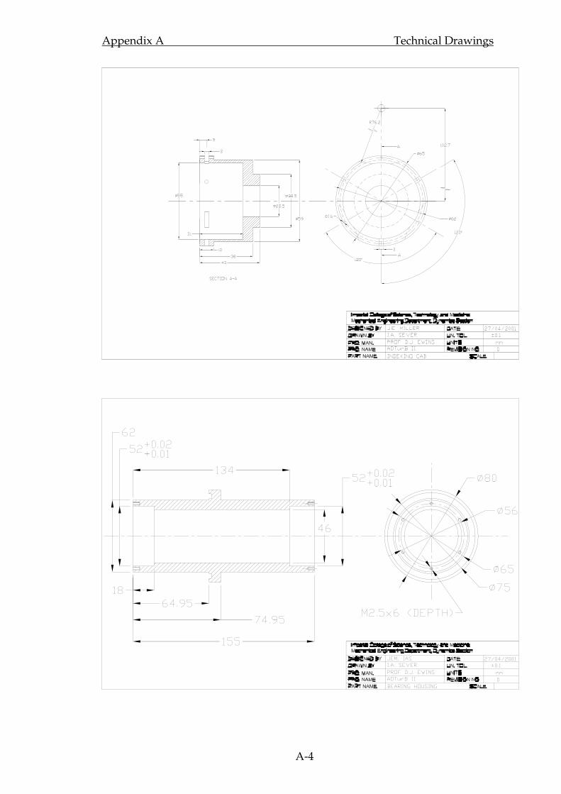
Appendix A Technical Drawings
A-4

Appendix A Technical Drawings
A-5

Appendix A Technical Drawings
A-6
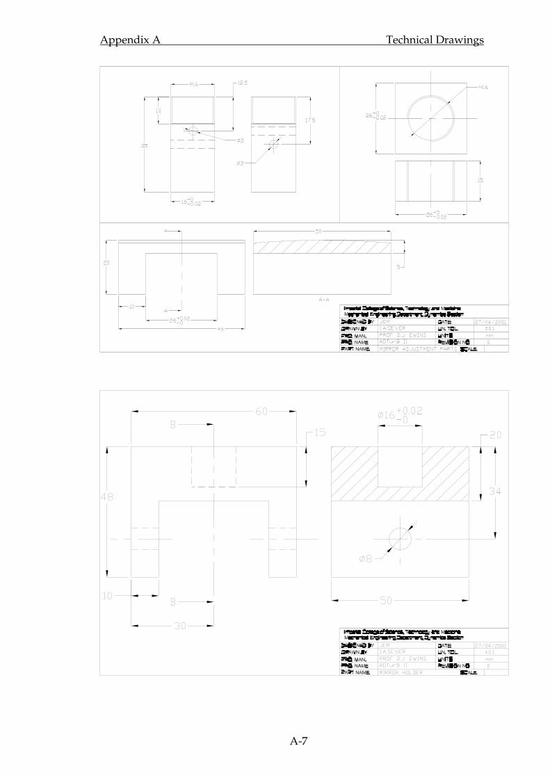
Appendix A Technical Drawings
A-7
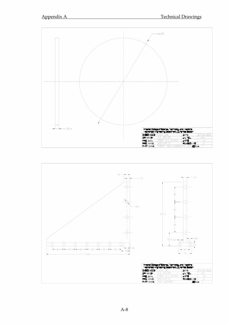
Appendix A Technical Drawings
A-8
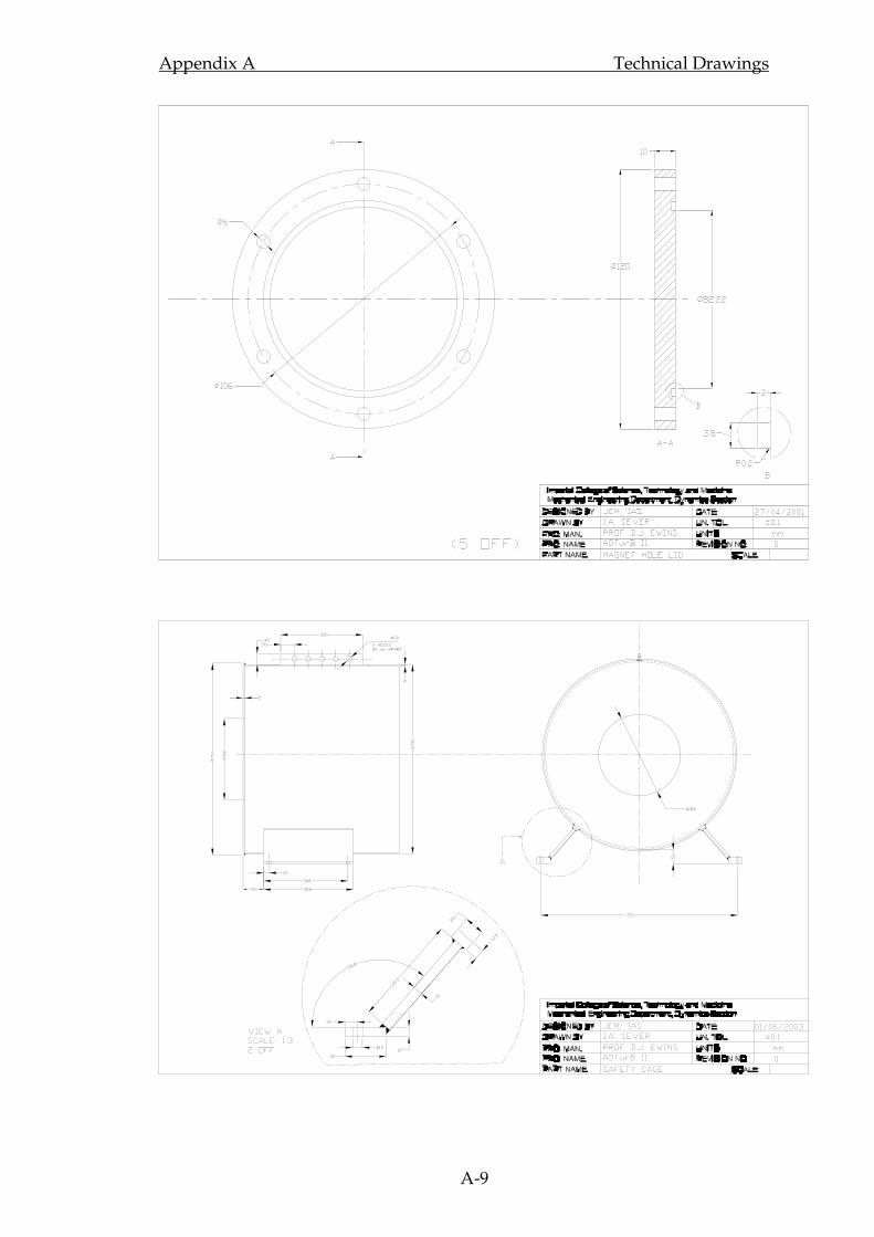
Appendix A Technical Drawings
A-9
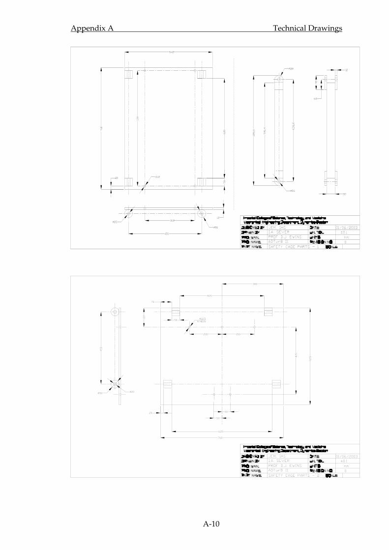
Appendix A Technical Drawings
A-10

Appendix A Technical Drawings
A-11
A.2 Blisk drawings
Blisk-1 - 1/2
Blisk-1 – 2/2
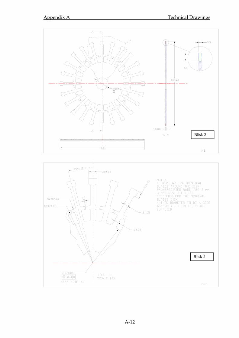
Appendix A Technical Drawings
A-12
Blisk-2
Blisk-2
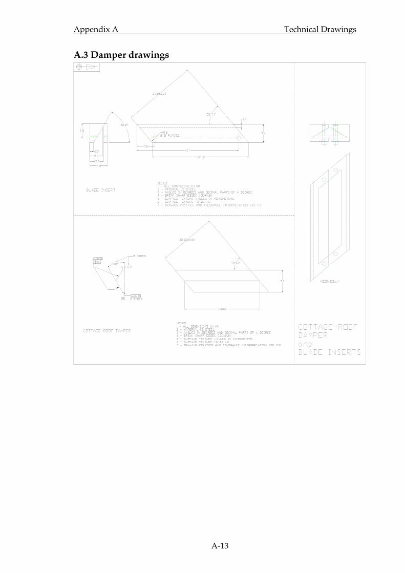
Appendix A Technical Drawings
A-13
A.3 Damper drawings
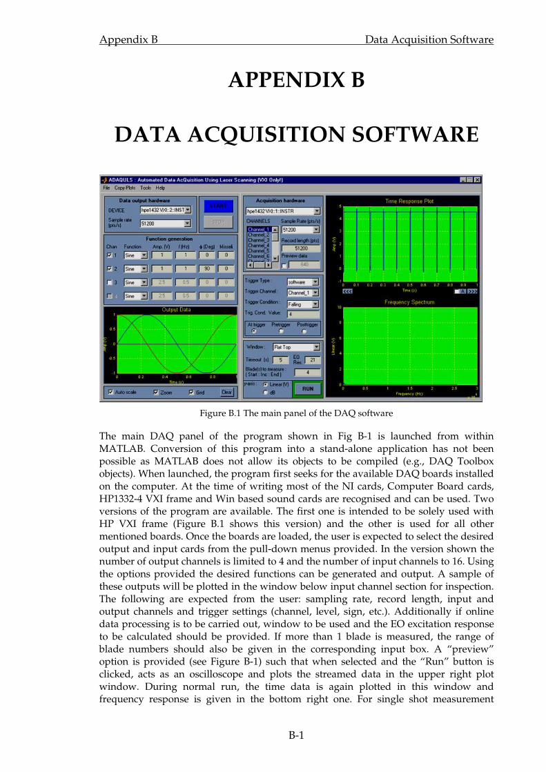
Appendix B Data Acquisition Software
B-1
APPENDIX B
DATA ACQUISITION SOFTWARE
Figure B.1 The main panel of the DAQ software
The main DAQ panel of the program shown in Fig B-1 is launched from within MATLAB. Conversion of this program into a stand-alone application has not been possible as MATLAB does not allow its objects to be compiled (e.g., DAQ Toolbox objects). When launched, the program first seeks for the available DAQ boards installed on the computer. At the time of writing most of the NI cards, Computer Board cards, HP1332-4 VXI frame and Win based sound cards are recognised and can be used. Two versions of the program are available. The first one is intended to be solely used with HP VXI frame (Figure B.1 shows this version) and the other is used for all other mentioned boards. Once the boards are loaded, the user is expected to select the desired output and input cards from the pull-down menus provided. In the version shown the number of output channels is limited to 4 and the number of input channels to 16. Using the options provided the desired functions can be generated and output. A sample of these outputs will be plotted in the window below input channel section for inspection. The following are expected from the user: sampling rate, record length, input and output channels and trigger settings (channel, level, sign, etc.). Additionally if online data processing is to be carried out, window to be used and the EO excitation response to be calculated should be provided. If more than 1 blade is measured, the range of blade numbers should also be given in the corresponding input box. A “preview” option is provided (see Figure B-1) such that when selected and the “Run” button is clicked, acts as an oscilloscope and plots the streamed data in the upper right plot window. During normal run, the time data is again plotted in this window and frequency response is given in the bottom right one. For single shot measurement

Appendix B Data Acquisition Software
B-2
individual channels can be observed separately by using direction buttons under the top-right plot window and can be copied to separate Matlab Figures using “Copy Plot” menu for further editing. For measurements performed for a range of speed values, a progress bar is displayed, as shown on the right. Via this bar the remaining measurement time, rotor speed, blade currently being measured etc. can be observed.
There are a number of tools provided under the “Tools” menu. These are: Motor Control, ODS, Band-Pass filter, Magnet Position tools and Preference setting window. Motor Control Tool: The user interface of the Motor Control Tool (MCT) is given on the right. Two test types, static and dynamic are available. When “static” option is selected the main panel does not expect any input from the MCT and all the fields seen in panel are disabled. With the selection of “Dynamic” option they are made available. When the “Run/STOP” pushbutton is clicked it initiates the communication with the motor when in “Run” state and shuts the motor down when in “STOP” state. With the use of MCT; Speed, Torque and Peak Torque can be set. The “Parameters“ section is provided for speed settings via which a constant value or a range of values can be entered. When a range is entered and the EO-ND crossing speed of interest is known, providing this value in the “Crossing speed” and selecting “Cluster” option clusters the speed values around this value resulting in a more efficient test session. Settings are transferred to the main panel upon clicking the “Apply” button. Magnet Position Tool
Via the Magnet Position tool shown on the left, the proximity of the magnet to the bladed disk can be adjusted. For a measurement session spanning a range of speed values, it is used internally if activated. It simply transmits the user specified “step” (i.e. distance) information through an RS232 cable to the stepper motor. “Home” is a user defined safe position for the magnet to be retracted in case of failure. Minimum distance allowed to the test piece is 2.5 mm. ODS Tool: The ODS tool shown on the right provides easy and quick ODS recovery and
visualisation opportunity on site. Three ODS options are provided for scans of type: circular, area and line. Upon selection of a choice, the relevant input boxes are made available and the others are disabled. The excitation frequency is directly taken from the motor speed reading, however this value can be fine

Appendix B Data Acquisition Software
B-3
tuned if necessary. Upon the clicking on the Plot button, the recovered ODS is plotted on the lower right plot window on the main panel. Band pass filter design
This panel provides the user with an easy and convenient way of preparing band-pass filters to be used in online EO response extraction. The filter can be applied to any number of channels and previewed before passed onto the main panel. There are a range of filters provided in the Method pull-down menu.
Preferences panel This panel is mainly intended for variable speed measurement session settings, however channel properties such as coupling and voltage range can also be set. Using the check boxes given in the upper part, the user can indicate which data to be saved. The storage matrices for unchecked parameters are not created and therefore more memory is made available. Time settings are very important in assuring the quality of the data and are structure dependent. For a very lightly damped system, one needs to provide a long enough pause between each successive speed change to make sure the steady state vibrations are reached.