DEFINING AND MEASURING ACADEMIC STANDARDS · PDF fileentitled Defining and Measuring Academic...

DEFINING AND MEASURING ACADEMIC STANDARDS FOR

HIGHER EDUCATION: A FORMATIVE STUDY AT THE UNIVERSITY OF SONORA

by

Manuel Jorge González Montesinos

______________________________

A Dissertation Submitted to the Faculty of the

DEPARTMENT OF EDUCATIONAL PSYCHOLOGY

In Partial Fulfillment of the Requirements For the Degree of

DOCTOR OF PHILOSOPHY

In the Graduate College

THE UNIVERSITY OF ARIZONA

2004

2

The University of Arizona Graduate College

As members of the Final Examination Committee, we certify that we have read the

dissertation prepared by Manuel Jorge Alberto Gonzalez Montesinos Martinez _____

entitled Defining and Measuring Academic Standards for Higher Education: A Formative

Study at the University of Sonora

and recommend that it be accepted as fulfilling the dissertation requirements for the

Degree of Doctor of Philosophy

___________________________________________ __________________ Dr. Darrell Sabers date

___________________________________________ __________________ Dr. Jannice Streitmatter date

___________________________________________ __________________ Dr. Jerome D’Agostino date

___________________________________________ __________________ Dr. Stan Maliszewski date

Final approval and acceptance of this dissertation is contingent upon the candidate’s submission of the final copies of the dissertation to the Graduate College. I hereby certify that I have read this dissertation prepared under my direction and recommend that it be accepted as fulfilling the dissertation requirement. _____________________________________________________________________ Dissertation Director date Darrell Sabers

3

STATEMENT BY AUTHOR

This dissertation has been submitted in partial fulfillment of requirements for an advanced degree at the University of Arizona and is deposited in the University Library to be made available for borrowers under the rules of the Library. Brief quotations from this dissertation are allowable without special permission provided that accurate acknowledgement of source is made. Requests for permissions for extended quotation from or reproduction this manuscript in the whole or in part may be granted by the head of the major department of the Dean of the Graduate College when in his or her judgment the proposed use of this material is in the interests of scholarship. In all other instances, however, permission must be obtained by the author. SIGNED: _______________________________________

4

ACKOWLEDGEMENTS My academic work has been guided by excellent Professors: Dr. Darrell Sabers

my trusted advisor and mentor since 1985, Dr. Jannice Streitmatter,

Dr. Jerry D’ Agostino, Dr. Stan Maliszewski and Dr. Chris Wood, members of my

doctoral committee; and from whom I have received the gift of professional trust. At the

Educational Psychology Department, I am grateful to Dr. Rosemary Rosser, Dr. Joel

Levin, Dr. Patricia Jones, Ms. Karoleen Wilsey, Ms. Carol Schwarnz, Ms. Toni Sollars,

Ms. Melinda Fletcher and Ms. Mary Marner. They have provided me with the finest

teaching, guidance, and academic support throughout my studies.

At the University of Arizona, Dr. Maria Teresa Velez, Ms. Sonia Basurto, and

Ms. Leticia Escobar helped ever so kindly to bring my studies to completion. At my

Universidad de Sonora, M.C. Maria Magdalena Gonzalez Agramont, M.C. Azalea

Lizarraga Leal, Dr. Enrique Velazquez, M.C. Enrique Gurrola Mac, Ing. Martin

Valenzuela B. and M.C. Benjamin Burgos collaborated effectively to make this project

possible. At the Universidad Autónoma de Baja California (UABC), Dra. Norma

Larrazolo Reyna, Dra. Graciela Arroyo Cordero, M.C. Luz Elena Antillón and Ocean.

Martin Rosas Morales provided sound advice and invaluable support during the data

collection phase. In Tucson I wish to thank Ms. Judy Maliszewski, Dr. Hugh Morris, Dr.

Francisco Marmolejo, Ms. Vanessa Chacon, Ms. Gabriella Theodosiou, Ms. Rena

Cuizon, Dr. Suzsanna Szabo, Ms. Sarah Bonner, Mr. Scott Marley and Mrs. Tennille

Marley. Their warm friendship and support is always remembered. In Caborca, Sonora,

Mexico, I must thank Mr. Jose M. Copado, Mr. Pedro Moreno, Mr. Ernesto Donnadieu

and their families. To all I say with heartfelt gratitude “Your guidance is my strength”.

5

DEDICATION

This work is dedicated to

My Wife, Addy Fatima,

Our Children, Jorge Manuel and Alejandro,

Our Grandchildren Jorge Manuel and Alexa Maria,

My Parents Manuel† and Lucila, and to my Sisters,

To my Grandparents†, Uncles and Aunts,

To Thayer and Carol† Erringer, and to

All of my Teachers through many years

6

TABLE OF CONTENTS

LIST OF TABLES……………………………………………………………………….8 LIST OF FIGURES……………………………………………………………………....9 ABSTRACT……………………………………………………………………………..10 CHAPTER 1: INTRODUCTION……………………………………………………….11

Background of the Study………………………………………………………...12

Purpose and Rationale…………………………………………………………...14

Methodological Approach……………………………………………………….15

Expected Results…………………………………………………………………17

Reasons for Studying Factorial Validity and Item Properties…………………...18

CHAPTER 2: LITERATURE REVIEW………………………………………………...20

Historical Background…………………………………………………………...20

Development of the Instrument………………………………………………….24

Conceptual Structure of the Examination………………………………………..26

The Basic Assumptions of EXHCOBA………………………………………….31

The Student Selection Model…………………………………………………….31

A Diagnostic of Academic Performance………………………………………...32

Development of the Conceptual Framework…………………………………….33

Standards Setting through Measurement Practice……………………………….33

CHAPTER 3: METHODS……………………………………………………………….34

Preparation of the 2004 Cohort Data…………………………………………….34

Statistical Methods……………………………………………………………….35

Exploratory Factor Analysis……………………………………………………..36

Process and Computer Implementation………………………………………….37

Confirmatory Factor Analysis…………………………………………………...42

Structural Models under Study…………………………………………………..44

Application of Item Response Theory…………………………………………...51

Basis and Application of the Rasch Model………………………………………53

7

Estimation of Item Difficulty and Person Ability Parameters…………………...55

Computer Implementation…………………………………………….................60

CHAPTER 4: RESULTS AND DISCUSSION OF STATISTICAL ANALYSES……..63

Academic Background Information……………………………………………..63

Gender and Age………………………………………………………………….64

Academic Trajectory…………………………………………………………….64

Average Results by EXHCOBA Structure………………………………………69

Descriptive Statistics on EXHCOBA Performance……………………………...72

Results of the Exploratory Factor Analysis……………………………………...73

Results of the Confirmatory Factor Analysis……………………………………91

Results of the Rasch Model Application………………………………………...97

IRT Results by Career Area Knowledge……………………………………….117

CHAPTER 5: REVIEW OF IMPLICATIONS AND CONCLUSIONS………………126

Discussion of General Implications…………………………………………….126

Implications for Current Testing Practice………………………………………128

Implications for Academic Standards Setting…………………………………..130

Design and Implementation of a Test Preparation Program……………………132

Definition of Performance Standards Expected at the University Level……….134

Design and Implementation of Alignment Studies……………………………..135

Recommendations………………………………………………………………136

Conclusions……………………………………………………………………..137

APPENDIX I…………………………………………………………………...............138

APPENDIX II…………………………………………………………………………..141

APPENDIX III………………………………………………………………………….144

REFERENCES…………………………………………………………………………162

8

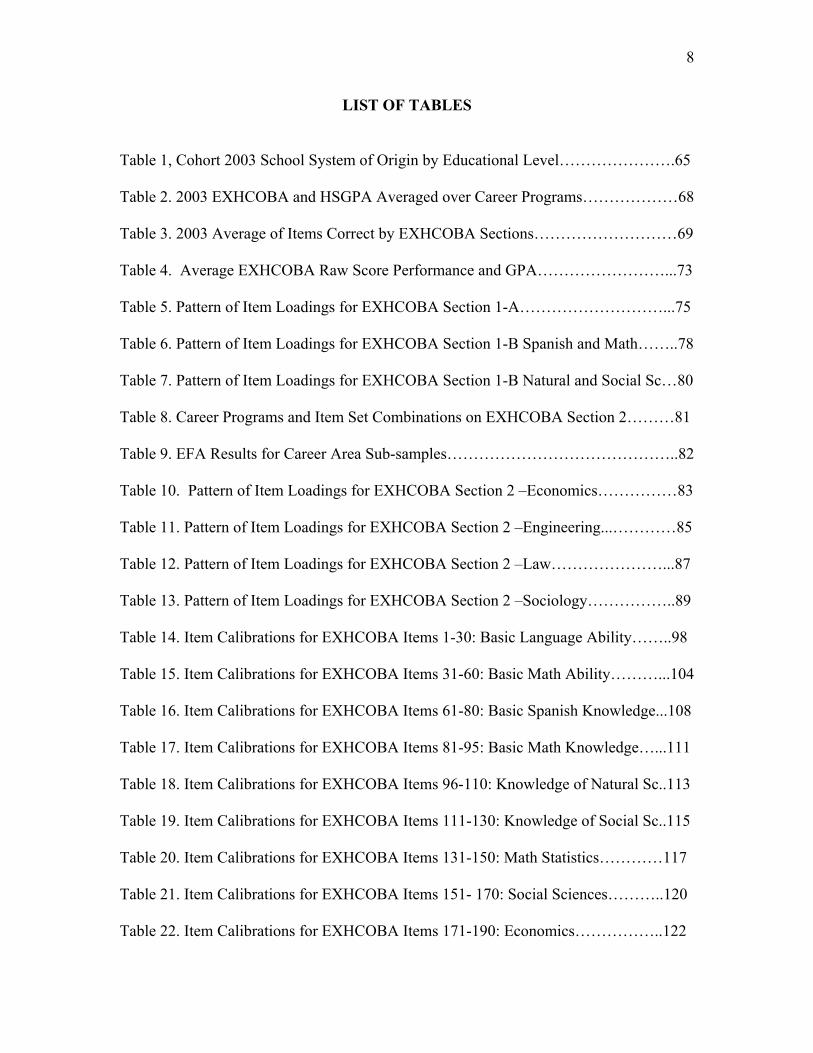
LIST OF TABLES

Table 1, Cohort 2003 School System of Origin by Educational Level………………….65

Table 2. 2003 EXHCOBA and HSGPA Averaged over Career Programs………………68

Table 3. 2003 Average of Items Correct by EXHCOBA Sections………………………69

Table 4. Average EXHCOBA Raw Score Performance and GPA……………………...73

Table 5. Pattern of Item Loadings for EXHCOBA Section 1-A………………………...75

Table 6. Pattern of Item Loadings for EXHCOBA Section 1-B Spanish and Math……..78

Table 7. Pattern of Item Loadings for EXHCOBA Section 1-B Natural and Social Sc…80

Table 8. Career Programs and Item Set Combinations on EXHCOBA Section 2………81

Table 9. EFA Results for Career Area Sub-samples……………………………………..82

Table 10. Pattern of Item Loadings for EXHCOBA Section 2 –Economics……………83

Table 11. Pattern of Item Loadings for EXHCOBA Section 2 –Engineering...…………85

Table 12. Pattern of Item Loadings for EXHCOBA Section 2 –Law…………………...87

Table 13. Pattern of Item Loadings for EXHCOBA Section 2 –Sociology……………..89

Table 14. Item Calibrations for EXHCOBA Items 1-30: Basic Language Ability……..98

Table 15. Item Calibrations for EXHCOBA Items 31-60: Basic Math Ability………...104

Table 16. Item Calibrations for EXHCOBA Items 61-80: Basic Spanish Knowledge...108

Table 17. Item Calibrations for EXHCOBA Items 81-95: Basic Math Knowledge…...111

Table 18. Item Calibrations for EXHCOBA Items 96-110: Knowledge of Natural Sc..113

Table 19. Item Calibrations for EXHCOBA Items 111-130: Knowledge of Social Sc..115

Table 20. Item Calibrations for EXHCOBA Items 131-150: Math Statistics…………117

Table 21. Item Calibrations for EXHCOBA Items 151- 170: Social Sciences………..120

Table 22. Item Calibrations for EXHCOBA Items 171-190: Economics……………..122

9

LIST OF FIGURES

Figure 1: Conceptual Structure of EXHCOBA…………………………………………26

Figure 2: Theoretical-Factorial Structure of EXCOBHA Part Ia……………………….28

Figure 3: Theoretical-Factorial Structure of EXCOBHA Part Ib………………………29

Figure 4: Theoretical-Factorial Structure of EXCOBHA Part II……………………….30

Figure 5: CFA Second Order Structural Model 1 of EXHCOBA Part 1a Variables……44

Figure 6: CFA Second Order Structural Model 2 of EXHCOBA Part 1b Variables……47

Figure 7: CFA Second Order Structural Model 3 of EXHCOBA Part2a Variables…….49

Figure 8: CFA Second Order Structural Model 3 of EXHCOBA Part2b Variables……50

Figure 9: CFA Second Order General Structure of EXHCOBA Part 2 sub-section……50

Figure 10: Map of Persons to Items from EXHCOBA Items 1-30……………………106

Figure 11: Map of Persons to Items from EXHCOBA Items 31-60…………………..110

Figure 12: Map of Persons to Items from EXHCOBA Items: 61-80………………….112

Figure 13: Map of Persons to Items from EXHCOBA Items: 81-95………………….112

Figure 14: Map of Persons to Items from EXHCOBA Items: 96-110………………...114

Figure 15: Map of Persons to Items from EXHCOBA Items: 111-130……………….116




10

ABSTRACT

Institutional efforts to organize the admissions process in several Mexican

universities have led to the adoption of standardized instruments to measure applicants'

initial academic qualifications for career programs. The University of Sonora, located in

four campuses throughout the state, initiated the administration of a college level

entrance exam in the fall of 1997. The Examen de Conocimientos y Habilidades Básicas

(EXCHOBA), developed in 1991, is the instrument employed for aiding the academic

and administrative agencies in making admissions and career placement decisions to date.

Drawing on current practice, this project develops a model for investigating the

alignment of the high school curriculum with the entrance examination by extracting and

clarifying the academic standards that derive from the official curriculum. Through a

series of statistical analyses on data from exam administrations, a working model for

defining the standards along with the instruments' sub-tests is proposed. The basis for a

system are then suggested to assist high school and university agencies and

administrators to interpret the results with a clear set of procedures for making curricular

and instructional decisions that will help improve the current rates of success in the

different career programs at the institution. In particular, the results obtained will lead to

a proposal to improve the academic advising and guidance programs that the Universidad

de Sonora is currently implementing to improve student retention and graduation rates in

its career programs.

11

CHAPTER 1

INTRODUCTION

Systematic testing and measurement practices in educational contexts in Mexico

are rather new and have depended mostly on standardized instruments of recent

construction (Backhoff, 1998). As usage of these devices is becoming more prevalent it

is now both necessary and justifiable to assess their measurement properties in particular

reference to officially published school curricula. In the state of Sonora located in the

northern section of the country, the practice of employing standardized tests instruments

was legally instated in 1997 through internal legislation passed at the state level

(UNISON, 1996). These legal decisions were based on the need for a uniform system

for student selection and placement into university career programs. Beyond the original

purpose that motivated this legislation, this project is presented as platform for advancing

testing and measurement practices to a different level. Namely, this project is based on

the fact that testing and measurement results can be profitably used to inform curriculum

development, instructional practices, and academic guidance activities at the high school

and university levels. The author takes the position that selected curricular content areas

should be officially treated as academic standards to be attained by curriculum and

instruction. These standards can be only be realistically defined through a technically

sound measurement system and the resulting interpretation of scores.

A formative study consists of a series of methodological trials to build a

customized system for analysis of a measurement situation where no precedent studies

exist. The aim the methodological exercise is to produce a working model that can be in

turned applied to systematize investigations in this relatively new educational research

12

area in Mexico. This approach is warranted in the case of the Sonoran High School

System and its relation with its corresponding state university for at least two reasons:

a) The practice of using standardized instruments to select students for university

programs is relatively recent in the state of Sonora, and b) No preceding studies have

taken on the task to compare the existing high school curriculum with the measurement

properties and factorial design of the instrument under use.

Consequently, the methods to be employed in the formative study are indicative

of two specific purposes:

a) to develop a model for assessing the correspondence of the curricular content

with the factorial structure of the instrument, and b) assessing the instrument’s sub-scales

by obtaining calibrations on item difficulty and ability of the examinees.

The combined application of these methods will in turn enable the researcher to

make a determination on the degree of alignment between the curricular content areas

and the instrument’s sub-scales. Based on the findings recommendations can then be

made as to the type of alignment adjustments that are required. However, the most

important result is that the curricular content areas can be successfully defined as

Academic Standards to be attained by the students showing also that the instrument to

determine such attainment is in fact available.

Background of the Study

This project focuses on developing a working model for studying the technical

definition and measurement specifications required to set academic standards for

admission and completion of university degree programs in a selected setting. The

University of Sonora is the largest publicly funded institution in the state and recently

13

declared an enrollment of 22,622 students in 31 career degree programs, (UNISON, PDI

2001, p.25).

Throughout its history the institution - founded in 1942- maintained an open

admissions policy based on a standard criteria of high school completion before

university enrollment. Beginning in 1997, the first attempts to place order in the

admissions process were put into effect by the adoption of a college level entrance

examination named "Examen de Habilidades y Conocimientos Basicos" – EXHCOBA.

The instrument was developed between 1986 and 1991 by a team headed by Eduardo

Backhoff Escudero of the University of Baja California (UABC) and Felipe Tirado

Segura, of the National Autonomous University (UNAM), (Backhoff & Tirado, 1992).

EXHCOBA’s adoption at the University of Sonora resulted from a process of

policy changes developed and mandated by the Academic Council between 1994 and

1996. It must be noted that this policy was implemented in order to develop an

institutional system to reduce enrollment in careers that were saturated with applicants.

While this purpose has been served, the university officially recognized the need for

advancing in this direction and determining the complete set of factors that interact to

produce the current rates which are 55.50% for completion of overall career programs of

study and 31.00 % for completion of all degree requirements leading to the official

degree conferral (UNISON, PDI 2001, p.30).

For the administrative period comprised between 2001 and 2005, the University

of Sonora produced an Institutional Development Plan (PDI) that addresses the

international and national contexts of the university and describes strategic programs for

meeting the challenges the institution presently faces. In this document the Universidad

14

de Sonora expressly recognized the need for developing and applying evaluation

processes that are valid, reliable, and methodologically sound to technically assess the

learning outcomes for students in all career programs, (PDI, p. 62). In the same context,

the Universidad de Sonora developed and began to implement in 2002 an Academic

Advising and Guidance Program denominated Tutorias Academicas. This program is

directly aimed at the early detection and remediation of undergraduate students’

academic deficits as they progress through the initial semesters of their career programs.

However, the relation of the academic difficulties experienced by entering students has

not yet been technically linked to the academic standards that the students are required to

meet to exit the high school system and to apply to their chosen career programs.

However, the relation of the academic difficulties experienced by entering

students has not yet been technically linked to the academic standards that the students

are required to meet to exit the high school system and to apply to their chosen career

programs. A detailed description of the instrument along with the main aspects of its

development is presented in Chapter 2 of this dissertation.

Purpose and Rationale

Continuing with the precedents set by current testing practices and in particular by

the use of EXHCOBA the research questions being addressed in this project are:

A) What are the academic standards that underlie the official high school

curriculum in the Sonoran Preparatory Sub-systems?

B) What are the technical properties of an instrument that measures these

academic standards?

15

C) How can the definitional and measurement results be applied by the high

school system to enhance curriculum and instruction?

D) How can the definitional and measurement results be applied by the university

to enhance its academic guidance efforts to improve current retention and

graduation rates in its career programs?

If this project is successful, the high school institutions involved as well as the

University of Sonora will benefit from a wealth of information derived from the

investigation of the actual relations of the current academic content and the initial

measurement efforts in place.

Methodological Approach

In order to shed light on the present situation, the project was divided in two

phases: a preliminary and a full project phase. During the preliminary phase, the

demographic and academic characteristics of university applicants taking the EXHCOBA

in the 2003 cohort are described as background context for the application of statistical

methods to the data generated by the examination.

During the full project phase the measurement properties of the instrument are

examined employing Exploratory Factor Analysis (EFA) and Confirmatory Factor

Analysis (CFA) in order to obtain a determination of construct validity. The procedures

employed are those available in the TESTFACT 4 program (Wood, Bock, Gibbons,

Schilling, & Muraki, 2003). The data to conduct this part of the analysis was obtained

from sub samples of the cohort of applicants that have taken the examination during the

months of May and June of 2004.

16

It is likely that the instrument functions as specified in its original structure (see

Figures 2, 3, and 4). However, it is precisely this internal structure that must be

determined in relation to the curricular content areas being covered in the high school

system. The resulting measurement dimensions are to be compared to the existing

standards in the high school curriculum. The working models will then produce an initial

basis for studying the areas of correspondence as well as discrepancies to compare the

actual alignment of the instrument with the curriculum content areas.

To conclude the full project phase, the alignment analysis of the instrument and

curriculum are extended to study the measurement properties of the specific EXHCOBA

subtests and in the measured dimensions.

In order to accomplish the above, the test result are analyzed by sub-test and items

employing one - parameter item response theory techniques (Embretson & Reise, 2000;

Wright & Stone, 1979). Namely, the item data are analyzed employing the Rasch

Model with the WINSTEPS Program, (Linacre, J. M., 2003). Once the measurement

properties of each of the EXHCOBA sub-scales are determined by this type of item

analysis, the university and the high school institutions involved will be in a better

position to examine and compare the academic standards being pursued at both levels.

As stated above, the exam results will be obtained from the Admissions Record

Data Base from the 2003 and 2004 applicant cohorts. Access to these records has been

secured by agreement with the Universidad de Sonora Admissions Committee. The

information of the data sets will be accessed and handled applying all the necessary rules

to insure the anonymity of the applicants. The Official Academic Standards will be

obtained from the curriculum of the Colegio de Bachilleres de Sonora (COBACH),

17

which is the largest state high school institution in the state with 25 campuses throughout

the state. Permission to study the standards alignment will be obtained from the central

administration of the state institution. It must be noted that the greater majority of

university applicants graduate from high school under the COBACH curriculum which

has been recently modified for the academic periods of 2003-04.

Expected Results

The expected results are as follows:

(1) A dialogue centered on Academic Standards will be initiated and carried out

between the academic authorities responsible for the curricular content areas and

instruction at the high school level and the university agencies responsible for defining

the admissions criteria.

(2) By examining the resulting conclusions the related university agencies will

have at their disposal a database that will enable them to develop and apply programs to

enhance the success rate of the students admitted to the different career programs.

(3) In particular, the University has begun an extensive academic guidance

program know as "Tutorias Academicas" (Academic Tutoring), which is to be eventually

offered to all students in the initial semesters of their career programs. The results by

knowledge domains can be applied to enhance the academic guidance efforts currently in

place by career programs.

(4) The academic authorities of the high school system will also have at their

disposal a database and a model for examining the curricular and instruction decisions

made by content area particularly for the junior and senior years. The model, once tested,

18

can be extended to aid in the decision-making procedures for semesters prior to the Junior

and Senior years.

Before proceeding to the next sections, it must be noted again that the original

purpose of the study was to define a set of procedures that afford technically sound

answers to the questions posed. Namely, once the system is in place for identifying and

measuring academic standards, the testing system can be profitably used to inform

educational practices in curriculum development and academic guidance programs.

This set of procedures will subsequently be treated as a working model for

conducting a full research program centered on the full definition of academic standards

in the State of Sonora. It is foreseeable that these research efforts will have to be

extended to the Sonoran educational system in grade levels preceding high school. In fact

that approach would be the ideal one. Nevertheless, this effort must begin at the high

school level because the only existing instrument to date the EXHCOBA was designed

and constructed to measure abilities upon completion of this particular level.

Reasons for Studying Factorial Validity and Item Properties

The EXHCOBA examination is a consolidated instrument. Its development and

usage have established content validity of the test subsections to a reasonable extent.

However, the documentation on file at the test development institute of the Universidad

de Baja California (UABC) indicates that while a considerable amount of information has

been gathered on the instrument’s performance, to this date no studies have been

conducted to study the factorial structure of the test (Antillon, 2002; Backhoff, 2001).

19

It seems logical that the next step in the development was to test the factorial validity of

the nine subtests. However, this dissertation project was based on the position that

studying the factorial structure of the test does more than gathering evidence for

establishing construct validity. A confirmatory analysis of the test structure based on

empirical data is a legitimate methodological tool that can be employed to technically

locate and define the academic standards that are implicit in a uniform curriculum. Once

results are obtained on the factorial structure of the nine subtests, a detailed study of the

item properties can be used to obtain calibrations of examinees’ actual abilities as well as

item difficulty indices. This in turn yields the basis for studying the actual alignment of

the instruments’ subtests with the curricular content areas that comprise the official

curriculum. The approach outlined here combines two solidly established measurement

techniques in to a systematic formal definition of academic standards which includes its

corresponding measurement apparatus.

20

CHAPTER 2

LITERATURE REVIEW

The main objective of this section is to review documentation from two stages of

development of educational assessment practices that are relevant to the current context

of the state of Sonora. It must be noted that this section briefly traces the relevant

antecedents of the introduction of standardized testing in the state but it will not render a

complete account of the history of educational evaluation in Mexico.

Historical Background

The practice of educational evaluation in Mexico and in the State of Sonora

follow parallel development stages because in the country educational policy has bay an

large been implemented following centralized directives that originate in the federal

agency responsible for designing and implementing educational policy, the Secretaria de

Educacion Publica (SEP) which is the national secretariat of public instruction.

For the purposes of assessing the publications that relate to educational evaluation

the project divides policy making and practice for evaluation in two stages. The first

stage includes the developments prior to 1990 in which educational evaluation was

carried out by educational agencies in Mexico largely as a self-contained series of

processes. During these stages evaluation criteria, procedures, and instruments were

applied in each state by educational institutions following an internal interpretation of

federally designed directives. By and large, the evaluation criteria for assessing

attainment of educational objectives were teacher assigned grades throughout the

different levels of schooling. That is, beginning in the elementary level, passing through

21

middle school, and ending with the preparatory level, students were required to complete

twelve years of instruction in which teacher assigned grades were the main indicator of

achievement. Beginning in the decade of the 70’s the Secretaria de Educacion Publica

(SEP) began administering National Evaluations with self-designed and self-appraised

evaluation processes with limited external criteria and lacking externally designed

measurement instruments and evaluation criteria. Nonetheless, by these practices the

states including Sonora amassed a considerable database containing information on

student’s aptitude and knowledge deriving from a uniform curriculum but with self-

generated indicators of student achievement. Nonetheless, as the main indicators were

teacher assigned grades within the different levels, grade point averages at the completion

of every level were taken to validly represent the required measures of educational

attainment. The vast majority of the information on student achievement handled by the

federal and state governmental agencies followed the same procedures of maintaining

grades by subject matter and grade point averages as the adequate indicator of

educational attainment.This manner of defining evaluation criteria for subject matter and

schooling subsystems is relevant because in the development of the instrument under

study the same conceptual structure was followed to make the examination parallel

subject matter division, sequences and general organization by schooling levels from

Elementary through High School.

This stage may be called for the practical purposes of this investigation the stage

of self-contained evaluation because the evaluation criteria were generated from within

the educational processes. This does not necessarily entail that previous practice was

undesirable. It merely represents a stage of development in which teacher and school

22

generated indicators of student achievement were the only evaluation tools available.

This situation must be understood in the context in which schooling practices are based

on a uniform curriculum that is delivered and regulated nationally by the Secretaria de

Educacion Publica (SEP). The uniformity in curricular content in the elementary,

secondary and preparatory levels affords a particular type of confidence in the teaching

practices that are so guided and therefore teacher assigned grades – assuming teachers

follow the curriculum − are taken to represent a valid measure of student educational

achievement.

During two decades − from 1960 to 1980 − there were important steps in the

development of psychometrics at the Universidad Autonoma de Mexico (UNAM) and at

the Instituto Politecnico Nacional (IPN) namely in the Schools of Psychology and

Medicine. However, the testing systems designed then were not extended to educational

levels outside these areas. Also, during the late 60’s several Mexican private institutions

of higher education began to utilize a Spanish version of the SAT called Prueba de

Aptitudes Academicas (PAA), developed at the Puerto Rico office of the College Board.

An important breakthrough in the history of educational evaluation in Mexico

came about with the foundation of the Centro para la Evaluacion de la Educacion

Superior A.C. known as CENEVAL. This national center began operating in 1994 under

the auspices of the largest public universities notably the Universidad National Autonoma

de Mexico (UNAM) as well as the Asociacion Nacional de Universidades e Instituciones

de Educacion Superior ANUIES. CENEVAL is registered as a national not for profit civil

association since April 28, 1994. Its mission is to organize educational testing and

evaluation systems for higher education institutions from the public and private sectors.

23

The institutions that contract the testing and evaluation services of CENEVAL do so on a

voluntary basis. The institutional decision to contract and apply the CENEVAL systems

conveys the institutional commitment of insuring the quality of their programs by

submitting to an independently designed formal evaluation program. The center began

to act as the entity officially responsible for organizing standardized testing systems to

regulate the admission processes for the most populated universities as Universidad

Autonoma de Mexico (UNAM) and also the Universidad Autonoma Metropolitana UAM

in central Mexico. The center marks a stage in which the practice of educational

evaluation would no longer be self contained as an external and independent entity

running standardized testing to diagnose achievement of exiting High School students.

For this purpose, CENEVAL produced the Examen Nacional de Ingeso (EXANI) which

is to date widely used by universities in central Mexico to organize admissions and

placement processes. This entrance and placement exam is available in two versions

EXANI-1 and EXANI-2, which have been designed to measure student achievement at

the high school level. The use of this instrument and the associated practices are not the

focus of the present study. Nonetheless, it is important to mention that these practices set

important national precedents for standardized testing in Mexico in the sector of public

education.

It must be noted that even before the large scale instruments above were available

for use, the EXHCOBA examination was already developed and employed by several

institutions. Thus, the EXHCOBA instrument which is the object of study in this

dissertation can be viewed as the precursor of large scale standardized testing in Mexico

(Martinez R., 2001).

24

Another turn of events recently modified educational evaluation practice in

Mexico. On August 8th 2002, the Mexican Congress passed a law creating the Instituto

Nacional de Evaluacion Educativa (INEE). This national institute is by law designed to

organize and conduct an educational testing program that will assess learning outcomes at

all levels throughout all levels of the country’s federal and state sub-systems. As national

testing begins to enter as a large scale practice, the national institute began in 2004 to

offer select results from national piloting studies at the elementary and secondary levels

Development of the Instrument

It was in this context that the need for an instrument measuring basic abilities and

knowledge possessed by students graduating from high school was addressed by the

developers of (EXHCOBA). It can be said that the instrument was constructed

anticipating the need for organized testing practices that employ independently developed

measurement instruments.

The EXHCOBA examination was developed based on initial research conducted

between 1986 and 1990 ( Backhoff & Tirado, 1992). The test development phase was

based on the analysis of examination results from a total of 14,166 students entering the

University of Baja California (UABC) seeking to pursue careers in 23 academic

departments and 53 career programs. The basic research included the administration of

several instruments which include: the Raven Test of Matrices, the Thurstone Test for

Primary Mental Abilities, and the Kuder Scale for Vocational Interest among others.

25

Based on the data analysis the authors decided to develop a college entrance

examination, which in turn produced the present EXHCOBA. This stage was

accomplished by an extensive item construction process. Item construction was based on

the content from the uniform curriculum applied in Mexico at the elementary, secondary,

and college preparatory levels.

After content and format analysis were completed, the instrument was produced

in computer format to enable electronic administration. The current version of the

instrument contains 310 multiple-choice items divided in two sections.

The first section has 130 items that must be answered by all students regardless of

their career choice and which are distributed as follows: 30 items for quantitative

abilities, 30 items for verbal abilities, 15 items for Spanish, 15 items for math, 20 items

for social sciences, and 20 items for natural sciences.

The second section comprises 9 content disciplines with 20 items each. The

content disciplines are: math for calculus, math for statistics, physics, chemistry, biology,

social sciences, humanities, language, and business administration. These disciplines are

in turn grouped in blocks of three each according to the area in which the career pursued

by the applicant belongs. The areas are denominated: 1) Economics and Business

Administration, 2) Biology and Chemistry, 3) Health, 4) Engineering, 5) Physics and

Mathematics, 6) Social Sciences and 7) Humanities. In this section students answer only

three blocks of 20 questions each according to the knowledge area of the career program

to be pursued. Hence, this last part contains 60 items grouped by knowledge area.

Adding the 130 items from the first section with the 60 from a selected knowledge area

any individual applicant must attempt to answer a total of 190 items (See Figure1 below).

26

Figure 1

Conceptual Structure of EXHCOBA*

BASIC ABILITIES

Elementary

Spanish

20 items

Mathematics

15 items

Natural Sciences

15 items

Social Sciences

20 items

Basic Knowledge by Area

Preparatory

Math

Calculus

20

Math

Statistics

20

Physics

20

Chemistry

20

Biology

20

Language

20

Social

Science

20

Humanities

20

Business

20

* The downward arrows indicate the sequence in which applicants progress through the examination sections

Language

30 items

Mathematics

30 items

Basic Knowledge

Secondary School

27

In sum, EXHCOBA is designed to measure:

1) Basic Abilities from the elementary school level

2) Basic Knowledge from the middle school level

3) Basic knowledge for an area of specialization from the high school level.

According to the developers the focus of the tests require from the examinees:

1) Notions and not specific precision in knowledge

2) Operative abilities such as execution and algorithms

3) Comprehension of written language and mathematics

4) Fundamental notions from selected disciplinary areas and related to

professional careers.

However, a formal psychometric approach to the structure of the examination

requires that the factorial structure underlying each subsection be examined with an

appropriate statistical procedure. For this reason the methods selected in this dissertation

attempt to examine the structure of the data as presented in the following figures, 2, 3,

and 4.

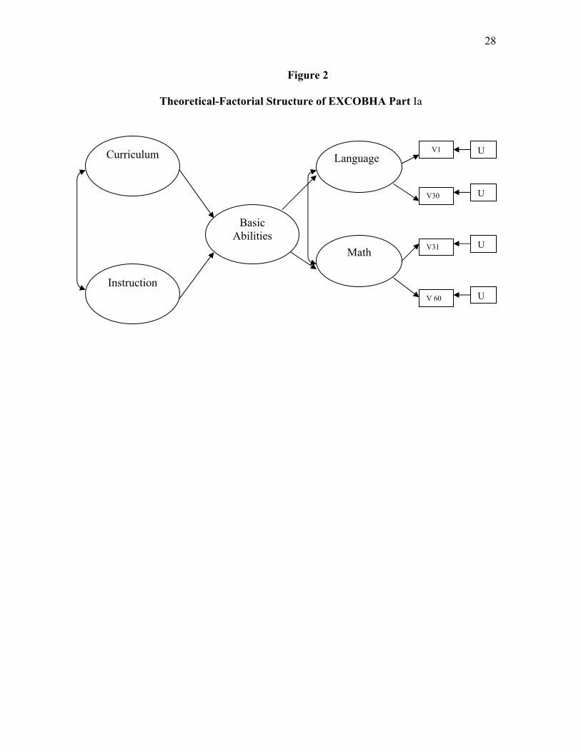
28

Figure 2

Theoretical-Factorial Structure of EXCOBHA Part Ia

Instruction

Curriculum Language V1

V 60

U

U

U

V30

V31 UMath

Basic Abilities

29

Figure 3

Theoretical- Factorial Structure of EXCOBHA Part Ib

Basic Knowledge

Instruction

Curriculum Spanish

Math

V61 U

U

U

U

V80

Natural Sciences

V125

V126

V130

U

U

U

V81

V95

V110 U

Social Sciences

30

Figure 4

Theoretical-Factorial Structure of EXHCOBA Part II

Curriculum

Instruction

U Math Cl

U Math St

U Physics

U Chem.

U Biology

U Lang.

U Soc. Sci.

U Human.

U

Area Knowl

Area Knowl

Area Knowl

Guidance

Area Knowl

Business

31

The Basic Assumptions of EXHCOBA Returning now to the origin of the EXHCOBA system as portrayed in the

literature, the educational assumptions that initially guided the developers’ effort were:

(1) Poorly grounded learning has little value for future learning and for this reason it

is appropriate and desirable to evaluate the basic learning that the student has

acquired through formal schooling from the elementary to high school sequence.

(2) Basic learning is required in order to achieve meaningful learning in post-

secondary schooling and to complete successfully a higher education program.

(3) Academic competencies are relatively stable and they develop over a long period

of time. Academic competencies do not change abruptly and this fact allows for

making predictive judgments based on test scores.

(4) EXHCOBA focuses on evaluating abilities to perform deductions, abstractions,

conceptualizations, and inferences of verbal and quantitative content that are

indispensable for the study and understanding of any given subject matter in

higher education.

The Student Selection Model

In order to develop a viable model for student selection the following criteria were

applied:

(1) A composite score based on the EXHCOBA score and High School GPA was

applied.

(2) The composite score alternative is based on the fact that admission exams have

limited predictive power.

32

(3) High School GPA is a suitable indicator of success at the university level and can

be a better predictor than admissions scores taken alone.

(4) The combination of these indicators improves the correlation with exam scores

obtained at the university level.

(5) The weighting scheme that resulted in the best combination for these variables is

65% for EXHCOBA scores and 35% for High School GPA.

(6) The application of the selection model resulted in a predictive validity coefficient

of 0.55 (Backhoff, 2002).

A Diagnostic of Academic Performance

An important implication of the selection process is that it provides a diagnostic

scheme for assessing the levels of academic performance with which the student attempts

a university level program. Since the process evaluates the actual possession of basic

knowledge and abilities, where there are measurable deficiencies in these, the acquisition

of new knowledge by students will be problematic. This situation if detected calls for

corrective action in two levels. Once the discrepancies between what is expected of the

student and what he or she can actually perform are identified, an institution can:

(1) Adjust its plans and programs of study to begin the educational process at an

adequate level.

(2) Remediate the academic deficiencies with special preparation and devise

systematic corrective actions until the deficiencies are solved in a measurable

manner.

33

Development of the Conceptual Framework

Intellectual abilities-broadly defined- results from combinations of knowledge,

capacities and effort. To locate a set of particular intellectual abilities at least two

questions require full answers:

(1) How many dimensions are required to describe individual differences in cognitive

task execution?

(2) What are the interrelations among dimensions of mental ability?

For the purposes of the present project, and following the approach initiated by

Backhoff and Tirado (2002), the two principal research questions guiding this

dissertation are a direct follow-up on the conceptual framework that underlies the

EXHCOBA effort. Namely, the questions concerning the identification of Academic

Standards underlying the official high school curriculum in Sonora converge on an

attempt to analyze the curricular and instructional results as these appear in the empirical

datasets produced by the EXHCOBA administrations to cohorts 2003 and 2004.

Standard Setting through Measurement

It has been noted that the systematic use of standardized instruments is rather recent

in the educational context under study. For this reason the literature review presented has

focused on the documentation generated mainly in relation to the initial use of the

EXHCOBA examination. However, in the United States an abundant body of literature is

available providing researchers with detailed technical analyses of the relationship

between educational measurement frameworks and the setting of academic standards.

Examples of this type research are found in Cizek (2001) among other sources.

34

CHAPTER 3

METHODS

The major section of this chapter provides a full description of the methodology p

along with the main technical requirements being met to conduct EFA, CFA, and IRT

analyses on the data obtained from the 2004 cohort of applicants. The general

requirements and procedures for each statistical technique are described along with the

computer programming appropriate for each type of analysis. Each case includes a

complete account of the decision making process to assess fit of the theoretical models of

EXHCOBA to the empirical data obtained from the 2004 cohort.

Preparation of the 2004 Cohort Data

The 2004 data set contains a total of 9,196 applicants to the University of Sonora.

The applicants are divided by the career program in which they seek admission. Each of

the segments contains a total of 190 variables per applicant corresponding to the number

of EXHCOBA items administered. As noted before, items 1 through 60 belong to section

1a of the test, items 61 through 130 belong to section 1b of the test, and items 131

through 190 belong to section 2 of the test. It must be noted that the 60 items in section 2

are presented to the applicants in combinations that correspond to the knowledge area of

the career program they have selected. The first step in applying the statistical methods

selected to obtain a representation of the constructs being measured by each subscale and

of the item properties of the instrument’s subsections, began by dividing the 2004 cohort

into in three randomly selected sub samples.

35

The random sampling procedure employed is available in the SPSS package

and it yielded the following sub samples: Sample 1 with n= 3051 analyzed with

exploratory factor analysis (EFA). Sample 2 with n= 3054 analyzed with confirmatory

factor analysis (CFA). Sample 3 with n=3091 analyzed with the one parameter item

response model (IRT). The purpose of analyzing the data under this sampling scheme is

to obtain a cross validation of the results.

Statistical Methods

Since the main objective of this dissertation was to devise and test a particular

methodology to identify and define the academic standards implicit in the high school

curriculum, a detailed description of the combination of statistical methods for this

purpose follows along with a technical justification for their use.

It must be noted that the approach taken focuses on a theoretical construct, which

is designated as the High School Curriculum as instantiated in the cohorts of university

applicants. For further clarification of the nature of this construct the reader is asked to

consider that the basic abilities and knowledge detected by the EXHCOBA instrument as

operating in the students’ measured academic backgrounds are part of a form of factual

curriculum as operationalized by their responses to the test item sets in nine sub-sections.

Given the above, the methodological task becomes the employment of the proper

statistical methods that will operationally define the sub-constructs of basic abilities and

knowledge factually possessed by the applicants. Once these sub-constructs are

identified through the statistical analysis of the measurement instruments’ data as

observed in the cohorts, it remains to be decided if these entities as identified actually

36

correspond to proper academic standards for higher education. The methods are

employed sequentially to attain a pattern of cross validation of the results obtained in

each approach. The cross validation is accomplished by applying the statistical

procedures to three randomly selected sub samples drawn from the 2004 Cohort. The

results of each procedure are then compared across the 3 sub samples to locate the

similarities and the differences in the structure of the data set.

The statistical groundwork resulting from the cross validation pattern becomes the

basis for a technical definition of academic standards as attained in practice and as

attainable in theory. The description of the statistical procedures that follows is based

largely on the literature of the computer implementation of the techniques (Bock et al.

1988); (Knoll & Berger, 1991). A similar application of the item factor analysis

techniques employed to assess teacher’s knowledge of subject matter exemplifies the

approach to factor analysis described and applied in this project (Hill, Schilling, &

Lowenberg, 2004).

Exploratory Factor Analysis

The first goal in the methodological approach is to identify the structure in the

EXHCOBA 2004 data set. The application of EFA procedures here is done in preparation

of the latent trait analysis performed with CFA. This aim is accomplished by

investigating the factual dimensionality of the data set. Exploratory factor analysis is

appropriate to identify the underlying dimension structure of a set of data. This is

accomplished by reducing a number of variables, 190 in the present case, to a smaller set

of factors that account for the covariation in the data set.

37

Drawing on the initial specifications, the instrument’s items are arranged into nine

subscales and these item groups should exhibit underlying dimensions. The idea behind

applying exploratory factor analysis is to determine the item sets that belong in each of

the dimensions that underlie the structure of the data sets. In the EXHCOBA examination

the factor analytic approach initially determines the number and the nature of constructs

being measured by the instrument’s subscales. In particular, it is of interest to obtain a

preliminary mapping of the basic ability and basic knowledge sub-constructs as these

emerge from the item response patterns in the 2004 data set. Drawing on the item

intercorrelations and following the ordering of the items in each subscale a pattern of

item sets emerges representing the factual curricular content being detected by the

instrument’s sub-sections. These patterns of item sets correspond in turn to the common

factors that account for the response patterns and a portion of the variance in the data set.

The common factors influence more than one observed variable, and in the

particular case these are expected to influence a number of item responses within a given

subscale. In the case of basic abilities and knowledge by content area these common

factors are also expected to be correlated among themselves. This calls for a particular

type of analysis in which the factors are plotted to be oblique in their geometrical

representation. This means that the common factors tend to influence each other as well

as the variables observed through the item responses.

Process and Computer Implementation

The package for computing the data analysis makes use of IRT estimation

procedures that employ all of the information in each examinee’s pattern of correct and

38

incorrect responses to the test items. These estimation procedures are called “full

information methods” because they compute the response information in all possible

occurrences and joint occurrence frequencies of all orders. That is all possible item

combinations, pairs, triplets, quadruples, etc., are considered information for the analysis

(Bock & Schilling, 2003).

The full information procedure in TESTFACT 4 (Bock , 2003) maximizes the

likelihood of the item factor loadings given the observed pattern of correct and incorrect

responses. The procedure solves the corresponding likelihood equations by integrating

over the latent distributions of factor scores assumed for the population of examinees,

called the θ distribution. The estimation method implemented in TESTFACT 4 is called

marginal maximum likelihood (MML) because the integration procedure employed by

the program is referred to as “marginalization”. This MML procedure has been shown to

produce feasible estimations for fitting item response models in multi-dimensional factor

spaces (Bock, Aitkin, & Muraki, 1988).

Since the EXHCOBA is a multi-dimensional test and the data set contains the

item responses given by the 2004 applicants coded “1” if the item was correctly answered

and “0” otherwise, the EFA procedure employed is the full information item factor

analysis based on inter-item tetrachoric correlations. This is a special requirement

because as the instrument’s items are dichotomously scored either correct or incorrect,

the inter-item correlations must be estimated in a manner that does not produce biased

estimates. The tetrachoric correlation meets this requirement and it is therefore used

throughout all of the subsequent analyses. Occasionally the tetrachoric correlation matrix

must be recalculated during the analysis in order to obtain a matrix with the property of

39

positive definiteness. In a smoothed inter-item correlation matrix the elements of the

diagonal are replaced with corrected roots and the non-positive roots are replaced with

either zero or a small positive quantity. Once the inter-item matrix is modified the

analytical procedure can be applied to obtain an initial representation of the structure of

the data derived from dichotomous variables.

The analysis is conducted in a sequence of steps requiring certain decisions to be

made at each step. The first step in performing EFA is the initial extraction of the factors

from an analysis of the inter-item tetrachoric correlation matrix. A common factor is a

hypothetical latent variable that is postulated to explain the covariation between two or

more observed variables.

The extracted factors will have two essential properties:

• Each factor will account for a maximal proportion of variance not

accounted for by other factors extracted in the process.

• Upon initial extraction each factor will be uncorrelated with all of the

previously extracted factors. If any of the extracted factors are in fact

correlated their relationships will be analyzed in subsequent steps of the

process.

• To obtain an accurate representation of the variables in their relationship

with the extracted factors, a rotation procedure is applied. In the present

case, VARIMAX rotation is selected to represent the variable factor

relationships maximizing the observed variance among the variables.

For present purposes the procedure described is implemented in the TESTFACT

program version 4, which uses the minimum squared residuals method (MINRES) to

40

extract the factors from the smoothed correlation matrix. The process and test description

that follow are taken from the TESTFACT manual (du Toit, Ed. 2003).

During the first phase of the procedure the item communalities are estimated.

These are defined as the squared multiple correlations between the observed variables, in

this case item responses and the set of factors that underlie the item sets. The estimated

communality is in turn the sum of squares of the loading of the observed variable on the

extracted factors. An item’s communality ultimately represents the proportion of

variance in the observed variable that is accounted for by the extracted factors common to

the variable. The item factor loadings represent the correlations between the observed

variable and the extracted factors. By general rule variable loadings above .30 are

considered meaningful for interpretation of the extracted factors. Loadings of .30 and

greater indicate that the item aligns with the factor where the significant loading occurs as

well as with other items that load on the same factor. It follows that the greater the

loading of an item on a factor there is a greater association between the item and the

construct it measures. In this manner by inspecting the pattern of item loadings on the

extracted factors, and by attempting to match the loadings with the basic abilities and

areas of knowledge that the item subsets were designed to measure, conclusions can be

reached about the factual statistical relationships between the item sets and the

hypothetical latent variables that the extracted factors represent in the analysis. However,

before the conclusions on the item loadings and item sets can be reached, it is necessary

to determine if the number of factors extracted adequately represents the structure of the

data. This is accomplished by conducting a hypothesis test on the number of factors.

41

The TESTFACT program provides a means for conducting the test as follows:

The initial run of the program is done with a hypothesized number of factors k. The

statistical test is then applied in the form:

H0: A k-factor model provides an adequate description of the data.

H1: A (k+1)-factor model provides an adequate description of the data.

As the program is run under the H1 number of factors specified, a χ2 statistic with the

corresponding degrees of freedom is obtained. Then the program is modified to run under

the H0 number of factors specified and the corresponding χ2 value and the degrees of

freedom are obtained.

The χ2 values with their respective degrees of freedom are then compared by

subtracting the value obtained under H0 from the value obtained under H1 and the

corresponding degrees of freedom are also subtracted. The resulting value is the test

statistic for testing a k factor model versus a k+1 factor model. If the resulting value is

significant, H0 is rejected and it is concluded that the number of factors in k+1 provide a

more adequate representation of the data.

Once the program is run under the conditions specified by the hypothesized

structure of the data in the item sets and the test results are significant it is then possible

to reach conclusions about the alignment of items and the number of factors tested. The

particular application of the procedures and tests just described to each of the EXHCOBA

sections are presented in the TESTFACT programs described in Appendix 1.

As noted before the exploratory phase of this analysis is run on a randomly

selected sub-sample of 3054 applicants that took the EXHCOBA in May of 2004 and the

hypothesized factor structures follow the conceptual framework of the two sections of the

42

instrument. The results of the statistical tests on the number of factors as well as item

loadings on the extracted factors are reported in the second section of Chapter 4.

Confirmatory Factor Analysis

The second step in the methodological approach to be tested involves the use of

confirmatory factor analysis (CFA) to approximate a representation of the latent traits

involved in the observed item response patterns. This statistical technique is properly

employed in a situation where the objective of a study is to test the hypothesis that a

particular linkage between a set of observed variables and a set of underlying factors does

in fact exist. As noted above, a factual curriculum exists as represented by the observed

variables measured by the EXHCOBA subsections, and it is reasonable to examine the

relationships between these variables as observed and the theoretical structure of the

instruments’ subsections. Drawing on theory it is postulated that basic abilities and

knowledge should be operationally present in students as result of their exposure to the

uniform high school curriculum and consequently a CFA application should identify as

factors these constructs or attributes.

Upon application, confirmatory techniques postulate either a full structural model

or a measurement model. The full structural model includes theoretical relationships

among latent variables as well as among observed variables and their corresponding

constructs. The measurement model is limited to depicting the relationships among

observed variables and their corresponding latent variables. Also, CFA models are first

order when the relationships postulated are hypothesized among latent and observed

43

variables only. Second order models include hypothesized relationships among latent

variables themselves as well as among latent and observed variables

In this project the application of CFA models the relationships among basic

abilities as latent variables and subtest item responses as observed variables, thus it is a

second order full structural model.

The primary task of the model testing procedure is to determine the goodness of

fit of the hypothesized models and the sample data. That is the structure of the

EXHCOBA subtests is imposed on the sample data as obtained from the cohorts, and the

CFA procedure tests how well the observed data fit the specified theoretical structures.

The description the model fitting process is summarized as:

Data= Model + Residual

Data represent score measurements related to the observed variables as derived

from persons comprising the sample,

Model represents the hypothesized structure linking the observed variables to the

latent variables, and

Residual represents the discrepancy between the hypothesized model and the

observed data.

In sum, the CFA application is properly employed to test the factorial structure of the

instrument as captured in the cohort’s sample data. The application is considered a first

order CFA measurement model as it tests the relationships of the observed data sets to the

postulated basic abilities and knowledge exhibited by the applicants upon test

administration.

44

For purposes of this study three second-order structural models are tested as

defined by the relationships presented in the following section.

Structural Models under Study

Following standard conventions and notation from structural equations modeling

this section describes the three models to be tested with a diagrammatic representation for

each along with the TESTFACT programming required for each testing procedure.

Model 1 corresponds to the basic abilities that result in students as a result of their

exposure to curriculum and instruction at the elementary school level.

Figure 5

CFA Second Order Structural Model with Observed Variables

EXHCOBA Part 1a

Basic Abilities

Language Ability

F1

V31-45 U31-45

D

U46-60 V46-60

V1-15 D

U1-15

V16-30 U16-30

Math Ability

F2

F3

45

It must be noted that this diagram differs from the complete model structure

presented before (see Figure 2), in that the relationships under study are restricted only to

latent variables hypothesized as attributes that operate at the level of the individual

examinees. For economy of space the observed variables are represented as sets of items

corresponding to the domain being tested rather than as individual variables. Also, error

or unique terms are represented by sets rather than as individual terms.

The model postulates the existence of a general second order factor denominated

“Basic Abilities”. This factor in turn influences two first order factors denominated

“Language Ability” and “Math Ability”. There are two disturbance terms corresponding

to each first order factor.

Before proceeding it must be clarified that the three models under study do not

contain factors corresponding to curriculum, instruction, and guidance per-se as the

original models do. This restriction on the number of hypothesized factors has been taken

in the interest of parsimony and because it can be assumed that basic abilities and

knowledge operationalized by the examinees’ observed responses to the item sets could

be assumed to stem from formal and systematic exposure to curriculum and instruction.

The TESTFACT programming for the first test run of Model 1 is reproduced in

Appendix II. In a general case the analysis proceeds in a series of steps based on the

results of the program in the initial run. The item to factor model is postulated following

a theory on the arrangement of the latent constructs as in the present case following

Figure 5. Model fit is evaluated by an overall procedure in which the focal point is to

determine the adequacy of the model in describing the sample data. This determination

involves several criteria which are presented below. The confirmatory procedure under

46

TESTFACT is called BIFACTOR and it specifies a general or domain factor and a k

number of factors to which the item subsets belong. The BIFACTOR procedure estimates

the loadings on a general factor with the presence of item-group factors. The items’

ordering as they are hypothesized to belong to each of the uncorrelated factors is

specified in the command file and the program is run to obtain the initial estimations.

The resulting output provides the basis for a goodness of fit test in which two

competing models are compared as follows:

H0: The item sets are indicators of a general factor and of k uncorrelated group

factors.

H1: The item sets are indicators of a general factor and of k+1 uncorrelated group

factors.

The competing models are run to obtain the χ2 statistics and the degrees of freedom

that correspond to each model. To test H0 versus H1 the difference between the χ2 values

and their respective degrees of freedom is computed. If the result is significant H0 is

rejected and it is concluded that the items belong sets to the group factors postulated by

the theory.

Up to this point the CFA procedure under TESTFACT has been described in

general terms following the basic statements of the programming presented for Model 1.

The technical specifications of usage and the decision making process in this section are

taken from the guidelines published in the program’s reference manual (SSI, 2003).

The next task in this section is to complete the CFA – TESTFACT methodology

by describing the computer programming for testing Models 2 and 3. These parts

complete the confirmatory factor analysis section of this project.

47

In the present series of analysis Model 2 consists of an attempt to capture the

structure of basic knowledge by subject matter domain that corresponds to part 1b of

EXHCOBA. These are taken as results of the students’ exposure to curriculum and

instruction at the secondary school level.

Figure 6

CFA Second Order Structural Model with Observed Variables

EXHCOBA Part 1b

Basic Knowledge

D

Spanish F1

Math F2

V61

V 95

U

U

U

U

V80

V81

Natural Sciences

F3

U

U

U

U

D

D

D

V 130

V 110

V 111

V 96

Social Sciences

F4

F5

48

The convention of representing observed variables as sets rather than individual

variables is also followed in the diagram above but the complexity of the model increases

as it postulates four separate subconstructs of basic knowledge corresponding to distinct

subject matter domains. The programming required is consequently modified to model

the influence of five factors: a general second order basic knowledge factor and four first

order factors for the four subject matter domains in the secondary school curriculum. The

corresponding program is presented in Appendix III.

Part 2 of the EXHCOBA consists of blocks of 60 items each. These blocks are

formed from combinations three sets of 20 questions taken from sub domains that

correspond to knowledge areas of the career program that the applicants choose to

pursue. Therefore, any 3 blocks of these 60 item sets is designed to measure specialized

area knowledge considered essential for attempting a career program at the university

level. In Sonora the high school system divides the student population by career tracks

upon students’ choice aided by a vocational counselor. Once this choice is made in the

junior year the students in each career track receive instruction in the specialized

knowledge area of the chosen track. This stage is considered to be the university

preparatory level in which students acquire the knowledge base from distinct but related

disciplines. The content disciplines are: math for calculus, math for statistics, physics,

chemistry, biology, sociology, economics and business, humanities and literature.

Following the classical distinction of exact sciences, natural sciences, social

sciences, and humanities, the specialized knowledge areas are distinct domains. It must

be noted that each subset in either the natural or the social sciences is considered to be

49

related by a common underlying factor that represents specialized knowledge pertaining

to specific area disciplines. The following diagrams represent these discipline areas and

their hypothesized relations.

Figure 7

CFA Second Order Structural Model with EXHCOBA Observed Variables

Part 2a

Math Cl U

UMath St

UPhysics

Chemist.

Biology U

U

Exact Sciences

Specialized Area

Knowledge Natural Sciences

50

Figure 8

CFA Second Order Structural Model with EXHCOBA Observed Variables

Part 2b

Sociology

Human Disciplines

Specialized Area

Knowledge

UPhilosophy

Literature

Humanities

U

U

UEconomics

Administration U

USocial Sciences

However, the examination in part 2 requires that each individual examinee answer

only a subset of 60 items composed from the combined knowledge areas and therefore

the actual structure of the data for this part takes on a general form as follows:

Figure 9

CFA Second Order General Structure of EXHCOBA 2

Items 130-150

Items 151-170

U

Disciplinary Career Area Knowledge

F1

D

Specialized Knowledge

F2

Items 171-190

U

U

51

Consequently the programming for testing this factor structure in Model 3 has

been modified to reflect the distribution of factors and observed variables in the

EXHCOBA part 2. The program is presented in Appendix IV.

With the above the methods section describing the CFA procedures applied in this

project is complete. The results of testing the three models as specified are presented in

Chapter 4.

Application of Item Response Theory

With the factors that operate in the EXHCOBA measurement system identified, it

becomes of interest to investigate the properties of each of the nine sub scales contained

in the instrument. The factors operationalize a technical definition of academic standards

but the instrument’s sub scales and item properties remain to be examined. The approach

for this task is the one parameter model known as Rasch Measurement. This exposition

of IRT principles and procedures follows the work of Hambelton and colleagues (1991).

Item response theory comprises a group of measurement techniques which

originated from the Rasch Model. The basic principles of the model are:

The performance of examinees on a test can be predicted by a set of factors called

latent traits or abilities.

The relationship between examinees’ item performance and the set of traits

underlying item performance is described by a monotonically increasing function

called the item characteristic curve.

52

The item characteristic curve plots the relationship between the examinees’ level

of ability and the probability of a correct response to an item. This implies that

examinees with higher ability levels have higher probabilities of a correct

response to a given item.

Item difficulty symbolized by δ, and the ability of examinees symbolized by β, are

sufficient elements to explain and predict performance in an examination because

these elements contain all the necessary information.

Since the abilities of individual examinees are taken by the technique as latent traits

and item difficulty is the parameter to be estimated, it becomes of interest to compare the

results of an application of the Rasch model to the EXHCOBA data with the factors

identified to operate in each subscale of the examination. Applying the technique in this

way yields calibrations for item difficulty and examinees’ abilities that are especially

relevant to the definition of the academic standards being identified by the EXHCOBA

measurement process.

IRT procedures for analyzing properties of examinations require that certain

assumptions be met:

The unidimensionality assumption specifies that only one ability is measured

by a particular set of items. This requirement is adequately met when the

presence of a dominant factor is detected influencing test performance in a set

of test data.

The local independence assumption specifies that when the abilities

influencing test performance are held constant the responses of examinees to

any pair of items are statistically independent.

53

The unidimensionality assumptions has an important implication for the analysis

of EXHCOBA test data because the instrument’s sub scales are designed to tap on to

specific and discrete sub sets of abilities at the level of the examinees. These sub sets

have been previously identified as operating factors by the CFA procedure. Therefore, the

results of the IRT analysis confirm from a different methodological stance that these sub

sets of abilities are in fact identifiable by more than one statistical procedure.

The local independence assumption when met proves that the items of the

EXHCOBA sub scales are in fact congeneric and that as sub sets they tap into the

specified sub construct; but it also demonstrates important features of the ability levels

detected in the test data. The property of local independence means that for a given group

of examinees with a fixed ability level the probability of a response pattern on a set of

items is equal to the product of probabilities associated with the examinees’ responses to

the individual items. This in turn implies that when the ability levels are identified and

held constant, individual items as variables become uncorrelated and are likely to be

independent as the basic ability underlying test performance has been partialled out.

Basis and Application of the Rasch Model

As noted before under the Rasch model item difficulty and ability level are the

only elements that account for test performance and it is the most stringent and

parsimonious approach. The model is represented in the formula:

Pi(βν) = e(β – δi)

1+e(β –δi) i = 1,2,…,n

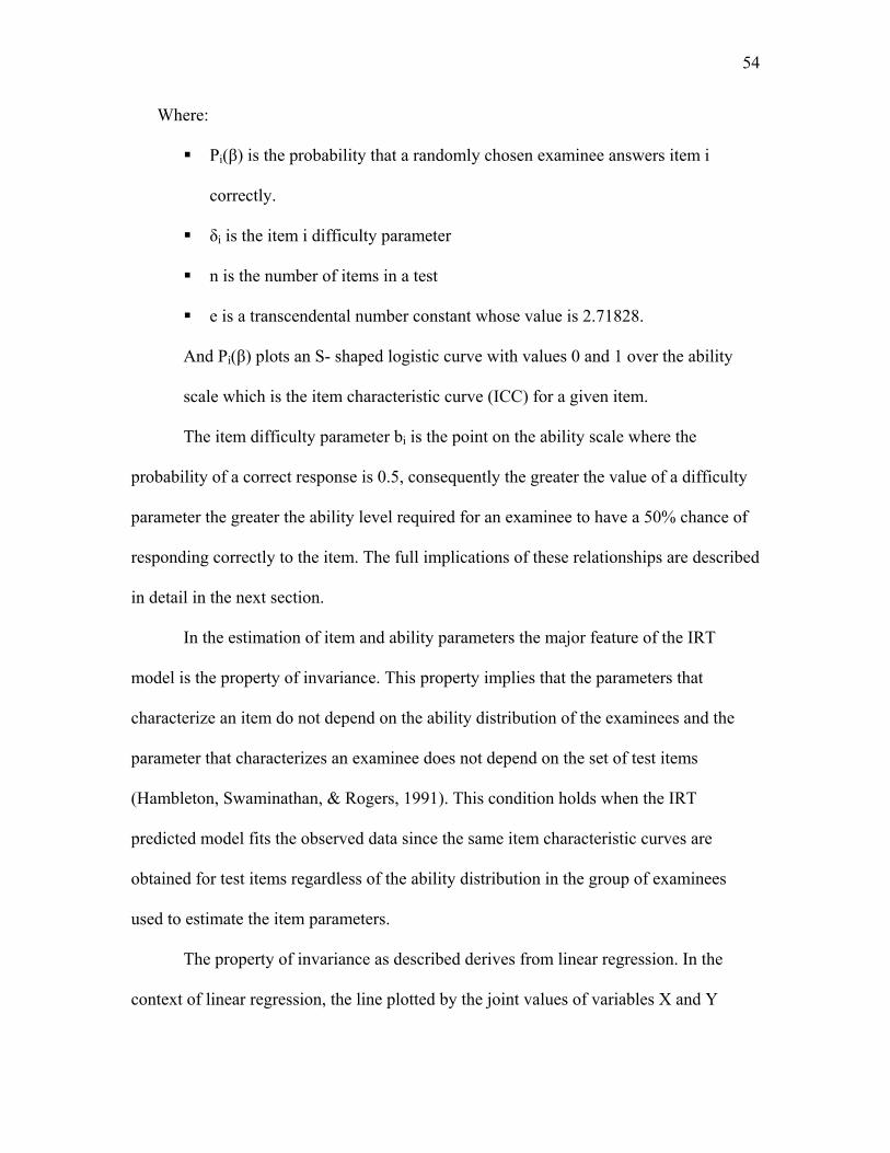
54

Where:

Pi(β) is the probability that a randomly chosen examinee answers item i

correctly.

δi is the item i difficulty parameter

n is the number of items in a test

e is a transcendental number constant whose value is 2.71828.

And Pi(β) plots an S- shaped logistic curve with values 0 and 1 over the ability

scale which is the item characteristic curve (ICC) for a given item.

The item difficulty parameter bi is the point on the ability scale where the

probability of a correct response is 0.5, consequently the greater the value of a difficulty

parameter the greater the ability level required for an examinee to have a 50% chance of

responding correctly to the item. The full implications of these relationships are described

in detail in the next section.

In the estimation of item and ability parameters the major feature of the IRT

model is the property of invariance. This property implies that the parameters that

characterize an item do not depend on the ability distribution of the examinees and the

parameter that characterizes an examinee does not depend on the set of test items

(Hambleton, Swaminathan, & Rogers, 1991). This condition holds when the IRT

predicted model fits the observed data since the same item characteristic curves are

obtained for test items regardless of the ability distribution in the group of examinees

used to estimate the item parameters.

The property of invariance as described derives from linear regression. In the

context of linear regression, the line plotted by the joint values of variables X and Y

55

predicts values of Y for any possible values of X. When a regression model holds the

same regression line will be obtained within any restricted range of the values of the

variable X in the regression equation. That is, in any sub-population of values of X the

slope and intercept values will be the same as long as the model fits the data. In the case

of item response models the same condition holds since these can be regarded as non-

linear regression models (Hambleton, Swaminathan, & Rogers, 1991, p. 19). However,

the property of invariance cannot be observed directly in the strict sense of the word. To

determine when invariance occurs in samples of test data the degree to which it holds in

observed test data can be assessed by determining the congruence of two or more sets of

estimates. If two samples of examinees of different ability are drawn from a population,

the comparison of item ability parameters can be taken as indication of the degree to

which invariance is holding in the particular case. The degree of congruence can be

approximated by obtaining the correlation between the two sets of estimates and by

examining the corresponding scatterplot.

Estimation of Person Ability and Item Difficulty Parameters

As stated previously in a one parameter model, the probability of an examinee’s

response to an item depends on the examinee’s ability β, and the item’s difficulty δ.

Given that both of these parameters are unknown the responses to the item are the

elements from which the estimation of the parameters is made. Since these elements are

observed, a probabilistic approach does not apply and the appropriate method for

estimation is the maximum likelihood approach.

56

Parameter estimation is also known as item properties and person abilities

calibration. The one parameter or Rasch model procedures for obtaining these

calibrations are described in detail by Benjamin Wright and Mark Stone. The exposition

below follows this source (Wright & Stone, 1979). The calibration procedure is

described in detail since it is a major aim of this project to obtain item and examinee

calibrations from the EXHCOBA examination data.

As described previously any ICC plots the probability of a correct response to a

test item combining the parameters βν for person ability and δι for item difficulty. To

construct the mathematical form for this plot these parameters are combined through their

difference (βν - δι). This difference in theory determines the outcome of the encounter of

an examinee ν with ability βν with an item ι of difficulty δι. However, a constraint is

required since the difference (βν - δι) can vary from -∞ to +∞ and the probability of a

successful response must be kept between 0 and 1. This constraint is placed by specifying

the difference (βν - δι) as an exponent of the natural constant e = 2.71828. The resulting

expression is written as e(βν - δι) = exp(βν - δι) which varies between 0 and +∞ and it is

converted to the interval between 0 and 1 by forming the ratio:

exp(βν - δι)/ [1 + exp(βν - δι)]

This ratio is then used to specify the probability of a successful response to an item by the

equation:

P{xνι = 1 | βν , δι.} = exp(βν - δι)/ [1 + exp(βν - δι)]

57

This equation is the Rasch model which specifies the logistic function that plots an ICC.

The model allows the estimation of βν and δι independently of one another in a way such

that the obtained estimates of βν are freed from the effects of δι and the estimates of δι are

freed from the effects of βν. This property was designated as “specific objectivity by

George Rasch who showed when developing the model that the measurements obtained

are in a linear scale with generality of measure (Rasch, 1960). Following the equation it

can be seen that when a person ν is of higher ability than the item’s difficulty δι the

difference (βν - δι) is positive and the person’s probability of success in the item is greater

than .50. As the person’s ability surpasses the item’s difficulty the positive difference

grows greater. Conversely, when the item’s difficulty is greater than the person’s ability

their difference is negative and the person’s probability of success is less than .50. With a

greater item difficulty the negative difference grows greater and the probability of

success approaches zero.

The units for representing estimates of βν and δι are called “logits” because a

person’s ability is calibrated as the natural log odds for succeeding on items that are

chosen to define the zero point in the scale. An item’s difficulty in “logits” is its natural

log odds for eliciting failure from persons with zero ability. The item difficulty and

person ability calibrations are performed under the Rasch model by a procedure called

PROX which exemplifies the transformations done to obtain the calibrations by hand

computation. The PROX procedure is described in detail here because it exemplifies

Rasch model and the results approximate calibrations under most computer programs that

follow the one parameter model (Wright & Stone, 1979, p. 28).

58

The PROX procedure assumes that person abilities (βν) are approximately

normally distributed with a mean M and standard deviation σ and that item difficulties (δι

are also more or less normally distributed with average difficulty H and difficulty

standard deviation ω. Thus when βν ~N (M, σ2) and δι ~N(H,ω2),for any person ν with

person score rν on a test of L items the ability estimation is given by the equation: bν = H

+ X ln [rν/(L-rν)] . For any item ι with item score sι in a sample of N persons the

difficulty estimation is given by the equation: dι = M + Y ln [(N- sι)/ sι] .

The coefficients X and Y are expansion factors which are required to follow the

difficulty dispersion of items in the case of X, and the ability dispersion of persons in the

case of Y. Specifically X= (1+ ω2/ 2.89)1/2 and Y = (1+ σ2/ 2.89)1/2 and the value 2.89 =

(1.7)2 comes from the scaling factor 1.7 which brings the logistic ogive into approximate

coincidence with the normal curve. This occurs because the logistic ogive values 1.7z are

never more than one percent different form the normal curve values of z.

The estimates bν and dι have standard errors which are :

SE(bν) = X [L/rν(L- rν)]1/2, and SE(dι) = Y [N/ sι(N- sι)]1/2.

The estimation method can be applied directly to observed item scores (sι) by calculating

the item score logit of item ι with the equation:

xι = ln [(N- sι)/ sι].

The item score logit of person ν is calculated with the equation:

yν = ln [rν / (L- rν)].

The expansion factors X and Y are then estimated by applying the equations

X = [(1+U/2.89)/(1-UV/8.35]1/2 for the person logit expansion factor, and

Y= [(1+V/2.89)/(1-UV/8.35)]1/2 for the item logit expansion factor.

59

In these equations 2.89 = (1.7)2 and 8.35 = (2.89)2 = (1.7)4, U is the item logit variance,

and V is the person logit variance. These variances are given by the formulas:

U = (Σ xι2 – Lx.2)/(L-1) and V = (Σyν2 – Ny.2) (N-1).

The parameter estimation is completed by setting the test center at zero so that H=0.

Then the parameters are obtained by: dι = M + Yxι = Y(xι –x.) for each item difficulty

and bν = H + Xyν = Xyν for each person’s ability.

The corresponding standard errors are given by the equations:

SE (dι) = Y [ N/sι (N- sι )]1/2 ~ 2.5/N1/2

SE (bν) = X [ L/rν(L- rν)]1/2 ~ 2.5/N1/2.

Finally the estimated person sample mean and standard deviation are given by M ≈ -Yx

and σ ≈ 1.7 (Y2 – 1)1/2.

Once the person and item parameters are estimated with the procedure above, the

next step is to assess the fit of the data to the model. With the actual estimations of bν and

dι taken from sample data, the difference between what the model predicts and the data

actually observed can be is obtained. These residuals from the model are calculated by

estimating the model expectation at each xνι from bν and dι and subtracting this

expectation from the xνι which is observed.

The model expectation for xνι is E { xνι} = πνι and the model variance is V{ xνι} =

πνι (1 - πνι), where πνι is obtained from : πνι = exp (βν - δι) / [1 + exp(βν - δι)]. The

standardized residual is obtained from: zνι = (X νι - πνι) / [πνι (1- πνι)]1/2.

If the observed data fit the model the standardized residuals must be more or less

normally distributed with mean zero and variance one.

60

Computer Implementation

It must be noted that the PROX procedure just presented is appropriate for hand

calculation of a person and item parameters and has been described as an approximation

of the actual process used when the procedure is run in a computer. The equivalent

procedure is called UCON and it is implemented in the WINSTEPS program developed

by John M. Linacre (Linacre, J.M., 2003). The program is designed to construct Rasch

measurement from the responses of a set of persons to a set of items. WINSTEPS begins

with a central estimate for each person measure and item calibration. These initial

estimates are obtained by an iterative version of the PROX procedure which is used to

reach a rough convergence to the observed data pattern. Then the UCON method is

iterated to obtain more exact estimates, standard errors, and fit statistics. The

implementation of the UCON procedure instantiates an unconditional maximum

likelihood and joint maximum likelihood methods for arriving at the final estimates of the

person and item parameters. The measures are reported in logits (log odd units) and the

fit statistics are reported as mean square residuals and also as standardized residuals with

N(0,1).

The estimation of fit starts by the program’s calculation of a response residual for

each person n when responding to each item i. This calculation produces an estimate of

how far the observed response departs from the model’s expected response given the

calibration of the person’s ability and the item’s difficulty. The response residual is

calculated with the formula:

yni = xni − Eni.

61

The residuals across persons and items are summarized in a fit statistic expressed

as a mean square fit statistic and as a standardized fit statistic with a z or a t distribution.

In the program’s output the fit statistics are reported as INFIT and OUTFIT

values for persons and items. The INFIT value is interpreted as weighted mean square

residuals which are sensitive to irregular patterns of response. This fit statistic is sensitive

to unexpected behavior affecting responses to items near the person’s measured ability

level. The INFIT statistic is calculated with the formula: INFIT = ΣZ2ni Wni / N.

The residuals are weighted by their individual variance to reduce the influence of

unexpected responses far from the person’s measured ability level or an item’s measured

difficulty level.

The OUTFIT statistic is the average of the standardized residuals across both

persons and items. This average is not weighted to produce estimates more sensitive to

unexpected responses far from the person’s measured ability level or an item’s measured

difficulty level. It is calculated with the formula: OUTFIT = ΣZ2ni / N. The OUTFIT

value is therefore interpreted as an unweighted mean square residual which is sensitive to

unexpected extremes in the observed response patterns. This fit statistic is sensitive to

outliers and more sensitive to unexpected behavior affecting responses to items far from a

person’s measure level.

For their interpretation the fit statistics are then compared to the following

criteria:

For INFIT: The mean square infit statistic (MNSQ) has an expectation of 1.

Values substantially below 1 indicate dependency in the observed data; while values

substantially above 1 indicate noise. A MNSQ of 1.0 indicates perfect fit. A value of 1.3

62

indicates the measure is suspect of misfit. Values above the 1.3 threshold are definite

misfits indicating noise or error in the data. Values less than 1.0 are also suspect of misfit

because they appear to fit too well.

In INFIT the standardized values appear as INFIT ZSTD. This is the infit mean

square statistic reported in natural logarithms. When this statistic ranges between -2 and

+2, the values are within an acceptable logit range for both persons and items. Values

greater than +2 are suspect of misfit and values less than -2 are also misfits.

For OUTFIT: The mean square outfit statistic (MNSQ) has also an expectation of

1.0. Values substantially less than 1 indicate dependency in the observed data; while

values substantially greater than 1 indicate the presence of outliers. A MNSQ of 1.0

indicates perfect fit. A value of 1.3 indicates the measure is suspect of misfit. Values

above the 1.3 threshold are definite misfits indicating noise or error in the data. Values

less than 1.0 are also suspect of misfit because they appear to fit too well.

In OUTFIT the standardized values also appear as OUFIT ZSTD. For this statistic

values between -2 and +2 are within an acceptable logit range for both persons and items.

Values greater than +2 are suspect of misfit and values less than -2 are also misfits.

For further interpretation of the values of INFIT and OUTFIT a measure is

considered to be Muted when it has unmodelled dependence, redundancy, or significant

error trends. This occurs when the values of the fit statistic are MSNQ < .08 or ZSTD <

-2. Conversely a measure is considered to be Noisy when it has unexpected unrelated

irregularities and extremes with values of MNSQ > 1.3 or ZSTD >+2.

The results of the person measures and item calibrations in from the EXHCOBA

2004 data for each of the nine subscales of the instrument are reported in Chapter 4.

63

CHAPTER 4

RESULTS AND DISCUSSION OF THE STATISTICAL ANALYSES

This chapter is divided in two major sections. The first contains preliminary

information describing the population of student applicants on academic background

aspects. An initial analysis of the performance on the EXHCOBA as observed in the

2003 cohort of applicants is included. This first part is presented merely as descriptive

background portraying the academic and social contexts in which the methodological

system is applied. The second major section of this chapter describes the results of the

data analysis based on the 2004 cohort’s performance in the EXHCOBA administration

Academic Background Information This initial section describes the main characteristics of the student population

with a focus on key indicators of educational background and trajectory. The content of

this section is taken from two main sources: (1) a database that contains the entrance

exam scores and grade point averages of the applicants in the incoming cohort, and (2) a

Student Entrance Survey administered to students that complete the admissions process.

Access to these databases has been provided by the Admissions Committee and the

Direction of Planning of the Universidad de Sonora. This section reviews these databases

with the aid of a publication that analyzes the data bases with interpretive comments of

the demographic data as well as the academic history of the applicants that completed the

registration process in full. (Gonzalez & Lopez, 2004)

During the 2003 admissions cycle 8814 high school graduates in Sonora applied

for admission to the Universidad de Sonora. A total of 5046 students were admitted and

64

registered for career programs distributed among the three Regional Units Campuses of

the university (Dirección de Planeación UNISON, 2003a).

The following information is gathered from the results of an Entrance Survey

(Encuesta de Ingreso) which is completed online by applicants at the time of registration.

This information has recently been compiled and published for educational research

purpose by the UNISON ( Direccion de Planeacion, 2004)

Gender and Age

In the 2003 cohort the gender of 5046 admitted applicants is 52% female and 48%

male. As for age the largest percentage occurs in the 17 -18 and19 -20 ranges with 44%

and 36% respectively. The remainder of the cohort corresponds to 10% in the range of

21-22, 3% in the range 23-24, and 7% in the range of 25 years and above. With regard to

marital status, 95% of the students are single which indicates that the majority can devote

a substantial amount of time to their studies. The remaining 4% indicated being married

and 1% live under common law marriage. It was also found that 96% of the students

report not having children, while 4% report they do. Again, this reinforces the notion that

the cohort’s situation is quite favorable for following a full course of studies in the career

university program for which they gained admission.

Academic Trajectory

With respect to scholastic trajectory the survey data indicate that most of the

cohort’s students completed their high school program in public institutions in each

educational level from pre-school up to high school and some completed their university

65

preparatory in a technical school. The following table lists the percentage of students that

completed their studies in either sector.

Table 1

Cohort 2003 School System of Origin by Educational Level

Educational Program Sector %

Pre-school Public 86 Private 14

Elementary Public 86

Private 14

Secondary Public 88 Private 12

Preparatory Public 79

Private 21

Technical Public 95 Private 5

It is important to note that the great majority of career program completed their

university preparatory or high school programs in institutions of the public sector. For

this reason the focus of the present study is the high school programs of that sector of the

Sonoran Educational system.

Regarding the scholastic trajectory of students a prime concern of this

investigation is the academic progress status upon entrance to the university system as

reflected by the high school grade point average (HSGPA) with which applicants exited

their respective preparatory programs. It must be noted that in the State of Sonora and

throughout Mexico, a students GPA is measured in a scale from 0 to 100 points with 60

66

points being the minimum score for exiting any given level of the system and progressing

to the next one. That is, a grade of 60 points represents the minimum passing score.

In the 2003 cohort the average HSGPA is taken as a rough indicator of the

scholastic trajectory of the typical student as it represents the collective assessment of all

teachers intervening in the instructional process of the student. It is granted that the GPA

by itself is not a pure measure of academic achievement or students scholastic aptitudes.

However, it is common practice to use it as a gross indicator of academic success.

Precisely for this reason it is of prime interest and concern to study the relationship of

GPA scores to other indicators of academic ability and achievement such as the

EXHCOBA scores.

For present purposes the Universidad de Sonora takes GPA scores as a general

indicator which reflects progress of students in the different levels of the educational

system as well as an overall indicator of students’ adjustment to academic life. (Gonzalez

L., 2004). In the 2003 cohort the highest HSGPA averaged over career programs was

observed in Medicine with 92 points and the lowest in Public Administration and

Agronomy with 77 points.

It must be noted that the 2003 cohort is the first one in which a systematic

analysis of scores obtained in the entrance examination EXHCOBA is performed. It must

be remembered that these scores are obtained with the first standardized instrument ever

selected for use at the Universidad de Sonora. For the purposes of this study, the analysis

must proceed under the working assumption that these scores are a stable indicator of

scholastic trajectory and adjustment to high school academic demands. In the cohort

under analysis the observed EXHCOBA scores are considered to be low with an overall

67

average of 50.06 points out of a possible 190 total points. The highest average score over

career programs was observed in students registering for the Physics Sciences career

program with an average of 71.54 points. The lowest average was observed in students

registering for the Mining Engineering program with 43.72 points on average obtained by

this subset of applicants. These performance scores are similar to those observed in

previous cohorts and therefore are taken to be stable indicators of the overall academic

trajectory with which the applicants seek admission and attempt to complete a

professional career program, (Gonzalez, L., 1999, 2000, 2004).

The Table 2 below presents in ascending order the average HSGPA and

EXHCOBA scores observed in applicants to professional career program in the cohort

under study.

68

Table 2

2003 EXHCOBA Scores and HSGPA

Average over existing Career Programs

Career Program EXHCOBA Average HGSPA

Mining Engineering 43.72 79.00 Law 45.19 78.66 Business Administration 46.56 79.75 Fine Arts 47.70 81.00 Chemistry-Biology 47.70 86.00 Agronomical Engineering 48.18 77.00 Media Communication 48.27 80.00 Biological Sciences 48.53 83.00 Information Systems 48.74 79.00 Geology 49.18 80.00 Mathematics 49.17 81.50 Public Accounting 50.53 83.00 Industrial and Systems Engineering 50.58 82.00 Psychology 50.94 83.00 Hispanic Literature 51.90 83.00 Finances 52.16 85.00 Computer Sciences 52.74 85.00 General Medicine 53.21 92.00 Economics 53.54 78.00 History 53.71 81.00 Social Work 54.30 82.00 Sociology 55.00 77.33 Public Administration 55.50 77.00 Civil Engineering 56.15 78.50 English Teaching 56.49 82.00 Electronics Technology 57.63 82.00 Nursing 58.46 84.00 Architecture 58.65 86.00 Linguistics 63.15 80.00 Physics Science 71.54 89.00

69

Average Results by EXHCOBA Structure

Disaggregating the proportion of items correct by each section of the entrance

examination shows that the knowledge area that has the highest observed proportion of

items correct is Basic Abilities corresponding to Elementary School instruction. The next

highest proportion of items correct was observed in Basic Knowledge corresponding to

secondary chool instruction. Finally, the lowest proportions of items correct were

observed in the areas of Knowledge by Career Specialty. These areas are taken as the

basic prerequisites for students attempting a professional career program. In these areas

the students are required to answer only 3 specialty subsections according to the

knowledge domain of the career program that they choose to attempt.

Table 3

2003 Average Proportion of Items Correct by EXHCOBA Sections

EXHCOBA Section Items Correct______No. of Items in Section

Basic Abilities

Verbal Abilities 60% 30 Quantitative Abilities 53% 30 Basic Knowledge

Spanish 53% 15 Mathematics 40% 15 Natural Sciences 55% 20 Social Sciences 50% 20 Knowledge by Career Area

Mathematics-Statistics 35% 20 Social Sciences 45% 20 Economics-Administration 45% 20 Mathematics-Calculus 40% 20 Biology 50% 20 Chemistry 35% 20 Physics 50% 20 Language 55% 20

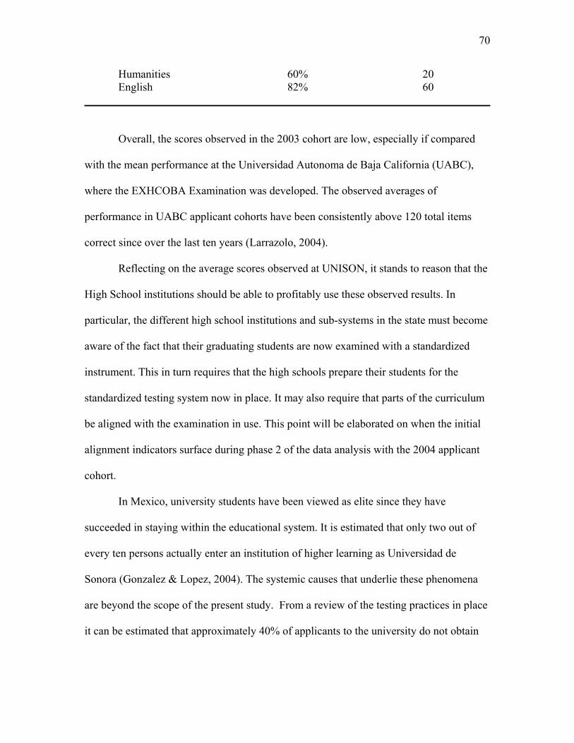
70

Humanities 60% 20 English 82% 60 ________________________________________________________________________

Overall, the scores observed in the 2003 cohort are low, especially if compared

with the mean performance at the Universidad Autonoma de Baja California (UABC),

where the EXHCOBA Examination was developed. The observed averages of

performance in UABC applicant cohorts have been consistently above 120 total items

correct since over the last ten years (Larrazolo, 2004).

Reflecting on the average scores observed at UNISON, it stands to reason that the

High School institutions should be able to profitably use these observed results. In

particular, the different high school institutions and sub-systems in the state must become

aware of the fact that their graduating students are now examined with a standardized

instrument. This in turn requires that the high schools prepare their students for the

standardized testing system now in place. It may also require that parts of the curriculum

be aligned with the examination in use. This point will be elaborated on when the initial

alignment indicators surface during phase 2 of the data analysis with the 2004 applicant

cohort.

In Mexico, university students have been viewed as elite since they have

succeeded in staying within the educational system. It is estimated that only two out of

every ten persons actually enter an institution of higher learning as Universidad de

Sonora (Gonzalez & Lopez, 2004). The systemic causes that underlie these phenomena

are beyond the scope of the present study. From a review of the testing practices in place

it can be estimated that approximately 40% of applicants to the university do not obtain

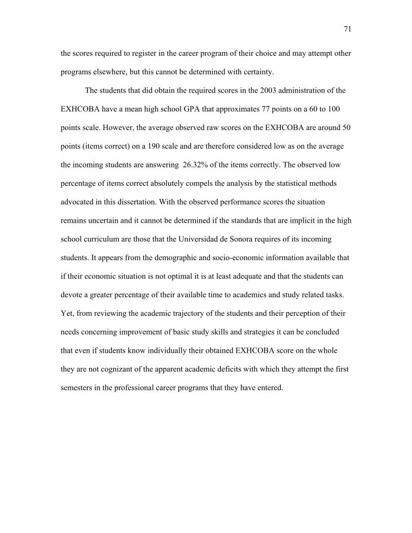
71

the scores required to register in the career program of their choice and may attempt other

programs elsewhere, but this cannot be determined with certainty.

The students that did obtain the required scores in the 2003 administration of the

EXHCOBA have a mean high school GPA that approximates 77 points on a 60 to 100

points scale. However, the average observed raw scores on the EXHCOBA are around 50

points (items correct) on a 190 scale and are therefore considered low as on the average

the incoming students are answering 26.32% of the items correctly. The observed low

percentage of items correct absolutely compels the analysis by the statistical methods

advocated in this dissertation. With the observed performance scores the situation

remains uncertain and it cannot be determined if the standards that are implicit in the high

school curriculum are those that the Universidad de Sonora requires of its incoming

students. It appears from the demographic and socio-economic information available that

if their economic situation is not optimal it is at least adequate and that the students can

devote a greater percentage of their available time to academics and study related tasks.

Yet, from reviewing the academic trajectory of the students and their perception of their

needs concerning improvement of basic study skills and strategies it can be concluded

that even if students know individually their obtained EXHCOBA score on the whole

they are not cognizant of the apparent academic deficits with which they attempt the first

semesters in the professional career programs that they have entered.

72

Descriptive Statistics on EXHCOBA Performance

Before presentation of the results on the instrument’s dimensionality and item

properties, it is necessary to have an overall picture of the applicants’ average

performance on the instrument on the nine subscales as well as on the total final score.

The descriptive statistics that follow are computed on the 2003 and 2004 cohorts of

students actually admitted and registered at the University of Sonora.

For the 2003 cohort N=5046 and for the 2004 cohort N= 5888, and the

comparative descriptive statistics are presented in Table 4. An inspection of the scores

reveals that except for minor variations the values in the nine EXCHOBA subscales as

well as over all performance on the instrument remain relatively stable for year to year.

This relative stability in admitted applicants’ performance has been observed in previous

cohorts (Gonzalez, L.,1999, 2000, 2004).

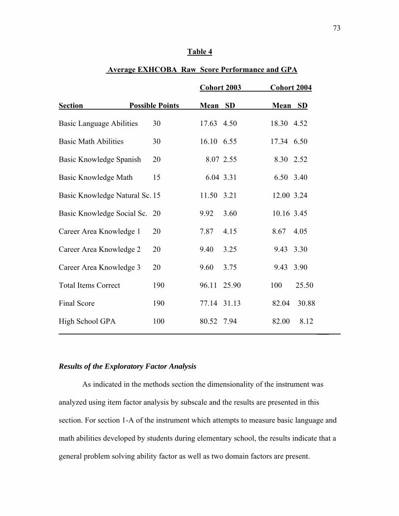
73

Table 4

Average EXHCOBA Raw Score Performance and GPA

Cohort 2003 Cohort 2004

Section Possible Points Mean SD Mean SD

Basic Language Abilities 30 17.63 4.50 18.30 4.52

Basic Math Abilities 30 16.10 6.55 17.34 6.50

Basic Knowledge Spanish 20 8.07 2.55 8.30 2.52

Basic Knowledge Math 15 6.04 3.31 6.50 3.40

Basic Knowledge Natural Sc. 15 11.50 3.21 12.00 3.24

Basic Knowledge Social Sc. 20 9.92 3.60 10.16 3.45

Career Area Knowledge 1 20 7.87 4.15 8.67 4.05



Total Items Correct 190 96.11 25.90 100 25.50

Final Score 190 77.14 31.13 82.04 30.88

High School GPA 100 80.52 7.94 82.00 8.12 ___

Results of the Exploratory Factor Analysis

As indicated in the methods section the dimensionality of the instrument was

analyzed using item factor analysis by subscale and the results are presented in this

section. For section 1-A of the instrument which attempts to measure basic language and

math abilities developed by students during elementary school, the results indicate that a

general problem solving ability factor as well as two domain factors are present.

74

In the TESTFACT 4 program the test for the appropriate number of factors in

the analysis is done in the following sequence:

H0: A k-factor model provides adequate description of the data.

Because the instrument’s design postulates two separate subscales for this section

the testing of the factor structure began hypothesizing two factors. The resulting values

under the 2-factor model are: χ2= 161096.72, DF = 2871.

The next step tests an alternative hypothesis:

H1: A k+1 model provides adequate description of the data.

The next run of the program was done hypothesizing three factors. The 3- factor

model resulted in a decrease of the test value to: χ2 = 160661.25, DF = 2813.

The statistical test is then applied by subtracting the obtained values and in this case the

result is:

161096.72 – 160661.25 = 435.47 with 2871−2813= 58 DF.

Since the critical value for χ2(50) = 76.154, at the α= .01 level and the obtained χ2 =

435.47 with 58 degrees of freedom , the result indicates that the three factor solution

represents the structure of this data set more adequately. The result may be explained by

the fact that language and math abilities acquired through the exposure to a uniform

elementary school curriculum are difficult to differentiate through answers to the test

items and therefore it appears that the response patterns are subsumed under one general

ability factor. With these initial results it is appropriate to explore the instrument’s

dimensionality to determine the correspondence of the test items with the actual factors

present in the data structure. VARIMAX rotation resulted in a distinct pattern of

loadings which is presented and discussed next. Inspection of the items loadings on the

75

extracted factors indicate a general ability factor as well as factors of language and

math ability being detected by the items as shown in Table 6 below.

Table 5

Pattern of Item Loadings for EXHCOBA Section 1-A: Basic Abilities

Item Factor 1 Factor2 Factor 3

ITEM1 .14 .32 .13 ITEM4 .33 .17 .11 ITEM5 .11 .33 .10 ITEM6 .30 .33 .13 ITEM8 .14 .30 .13 ITEM12 .14 .41 .10 ITEM14 .43 .17 .13 ITEM21 .13 .30 .24 ITEM22 .32 .11 .13 ITEM24 .38 .24 .19 ITEM31 .17 .16 .36 ITEM32 .32 .17 .27 ITEM33 .08 .21 .33

ITEM34 .39 .14 .24 ITEM35 .14 .19 .32 ITEM36 .33 .22 .28 ITEM37 .14 .17 .32 ITEM38 .30 .19 .32 ITEM39 .11 .16 .44 ITEM40 .29 .16 .35 ITEM41 .21 .30 .33 ITEM42 .35 .09 .34 ITEM43 .20 .10 .43 ITEM44 .37 .07 .32 ITEM45 .24 .11 .41 ITEM46 .17 .08 .40 ITEM47 .35 .04 .34 ITEM48 .18 .08 .41

ITEM49 .36 .21 .23 ITEM50 .15 .13 .35

ITEM51 .36 .15 .28 ITEM53 .28 .13 .35 ITEM54 .15 .27 .35 ITEM55 .17 .17 .41 ITEM56 .14 .14 .36 ITEM57 .36 .15 .26 ITEM58 .08 .16 .36

ITEM59 .25 .24 .31 ITEM60 .06 .16 .42

76

For economy of space only the items with at least one significant loading are

reported. Values in bold are added to emphasize the highest loading of each item.

Inspection of the loading pattern reveals the presence of a primary general factor with

items from the language ability and math ability subscales loading on this factor. The

fact that six language ability items and ten math ability items load under this general

factor strongly suggests that this factor represents a general problem solving ability. This

interpretation is supported by the contention that in general math ability items tend to

associate more with problem solving than language ability items. In this case the pattern

is clear as ten math items appear to be associated with the problem solving ability while

only four of the language items are associated with this general factor.

A noticeable language pattern is clear as items 1, 5, 6, 8, 12, and 21, which belong

to the language ability subscale, appear with bold loadings under factor 2. This suggests

the presence of a distinct language ability factor that is being detected by the language

subscale which is composed of items 1 through 30.

The definitive indication of a clear pattern becomes evident by considering the

loadings beginning with item 31. According to the instrument’s conceptual structure,

item 31 is the first item of the math ability sub scale. From this point on it can be clearly

seen that all the remaining items load under factor 3. This warrants the conclusion that

this factor represents math ability. It must be noticed that 13 of the 30 items on the

subscale load under the math ability factor.

The pattern of loadings under discussion is at least initially consistent with the

instrument’s theoretical structure. The loading pattern exemplifies item properties as

77

attempting to measure a common construct named general problem solving ability with

two distinct sub constructs named language and math ability.

Section 1-B of the instrument which comprises 70 items related to basic

knowledge acquired through exposure to secondary school curriculum contains an

assortment of items related Spanish, Math, Natural Sciences, and Social Sciences.

The arrangement of the items in that order required that the EFA program be

modified to explore the dimensionality of the Spanish and math items ina subscale

including of items 61 through 80 for basic knowledge of Spanish, and another subscale

including items 81 to 95 for basic knowledge of math. In the same manner the analysis

program was modified to run on items 96 through 110 representing a subscale of basic

knowledge of natural science and items 111 through 130 as a separate subscale

attempting to measure basic knowledge of social sciences.

The first run of the program on the items sets of Spanish and Math basic

knowledge was done hypothesizing the presence of one factor to account for the structure

of the data. This program run resulted in the following test values χ2 = 77543.87, DF=

2980.

The next run hypothesizing two factors resulted in χ2 = 72113.25, DF= 2946.

The test for the number of factors is then 77543.87 − 72113.25 = 5430.56, with 2980 −

2946 = 34 degrees of freedom. By this result the one factor hypothesis is rejected since

the critical value is χ2(34) = 56.061 at α = .01, concluding that two factors are more

appropriate to account for the structure of the data.

78

With the above conclusion the next logical step is to explore the correspondence

of the item sets with the extracted factors. After applying VARIMAX rotation, the item

loadings show the patterns found in the data as presented in Table 6 below.

Table 6

EXHCOBA Section 1-B: Basic Knowledge of Spanish and Math

Pattern of Item Loadings

Item Factor 1 Factor2

ITEM61 .42 .27 ITEM62 .09 .01 ITEM63 .02 .01 ITEM64 .32 .26 ITEM65 .28 .24 ITEM66 .28 .34 ITEM67 .38 .22 ITEM68 .36 .29 ITEM69 .31 .29 ITEM70 .36 .24 ITEM71 .21 .12 ITEM72 .14 .15 ITEM73 .22 .12 ITEM74 .17 .15 ITEM75 .22 .14 ITEM76 .23 .18 ITEM77 .17 .10 ITEM78 .22 .23 ITEM79 .24 .21 ITEM80 .24 .17 ITEM81 .10 .10 ITEM82 .18 .13 ITEM83 .26 .23 ITEM84 .21 .07 ITEM85 .17 .12 ITEM86 .30 .22 ITEM87 .33 .25 ITEM88 .35 .29 ITEM89 .27 .23 ITEM90 .25 .27 ITEM91 .42 .27 ITEM92 .09 .01 ITEM93 .02 .01 ITEM94 .32 .26 ITEM95 .28 .24

79

Most of the items bold loadings appear under factor 1 and only item 66 loads on

factor 2. In this result no discernible pattern of loadings can be detected in Table 6.

However, modifying the original expectation to two general knowledge factors allows a

better interpretation. Notice that items 61, 64, 67, 68, 69, and 70 belong originally to

basic knowledge of Spanish while items 86, 87, 88, 91, and 94 belong originally to basic

knowledge of math. This is an indication that in this data set the two knowledge domains

are not so distinct. This might well be because the items are worded in such a way that

general problem solving ability factor is applied by the respondents. This possibility can

be tested after the item sets are examined in their final groupings after the rest of the item

diagnostics.

The plausible explanation for this second result is that basic Spanish knowledge

and basic math knowledge align under a general knowledge factor rather than under the

two distinct cognitive domains originally expected.

The analysis for the next two item sets also required a separate program run to

explore the dimensionality of the knowledge of natural science subscale (items 96

through 110), and the knowledge of social science sub scale ( items 111 through 130).

The program run was performed hypothesizing a two factor structure and the

result gives a χ2 = 73412.24, DF=2946, P=0.00. Although an attempt was made to test the

hypothesis of a one factor structure, the result was not obtainable as the program output

indicated a singular matrix under the one factor hypothesis. With this limitation imposed

by particularities of this section of the data set, the two factor structure is retained

although in a speculative way.

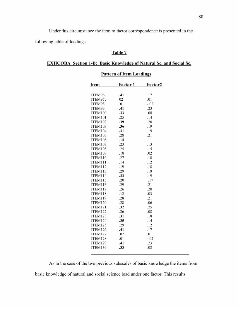
80

Under this circumstance the item to factor correspondence is presented in the

following table of loadings:

Table 7

EXHCOBA Section 1-B: Basic Knowledge of Natural Sc. and Social Sc.

Pattern of Item Loadings

Item Factor 1 Factor2

ITEM96 .41 .17 ITEM97 . 02 .01

ITEM98 .01 -.02 ITEM99 .41 .23 ITEM100 .33 .08 ITEM101 .25 .14 ITEM102 .39 .20 ITEM103 .36 .19 ITEM104 .31 .19 ITEM105 .28 .21 ITEM106 .14 .11 ITEM107 .23 .13 ITEM108 .25 .15 ITEM109 .18 .02 ITEM110 .27 .18 ITEM111 .14 .12 ITEM112 .19 .18 ITEM113 .29 .19 ITEM114 .33 .19 ITEM115 .20 .17 ITEM116 .29 .21 ITEM117 .26 .20 ITEM118 .12 .03 ITEM119 .28 .21 ITEM120 .28 .06 ITEM121 .32 .25 ITEM122 .26 .08 ITEM123 .31 .18 ITEM124 .35 .14 ITEM125 .29 .12 ITEM126 .41 .17 ITEM127 .02 .01 ITEM128 .01 -.02 ITEM129 .41 .23 ITEM130 .33 .08

As in the case of the two previous subscales of basic knowledge the items from

basic knowledge of natural and social science load under one factor. This results

81

reiterates the finding that a single general knowledge factor appears to be present in the

data set from section 1-C of the instrument.

The analysis for section 2 of the instrument has substantial changes. It focuses on

the last 60 items that each applicant responds in combinations that are arranged to the

career program each applicant pursues.

For the analysis the section 2 data sets were divided in the following order:

Table 8

Career Program and Item Set Combinations on EXHCOBA Section 2

Career Area Item Sets No. of Applicants

Economics and Administration 131-190 1 562

Chemistry and Biology 191-250 2 233

Health Sciences 211-270 3 372

Engineering and Science 191-210, 231-270 4 552

Architecture 191-210, 251-290 5 119

Law and Literature 151-170, 271-310 6 576

Sociology and Psychology 131-170, 271-290 7 625

1 Items sets: Math-Statistics, Social Science, Economics and Administration.

2 Item sets: Math-Calculus, Biology, and Chemistry.

3 Item sets: Biology, Chemistry, and Physics.

4 Item sets: Math-Calculus, Chemistry, and Physics.

5 Item sets: Math- Calculus, Physics, and Language.

6 Item sets: Social Sciences, Language, and Humanities.

82

7 Item sets: Math-Statistics, Social Sciences, and Language.

Consequently separate exploratory factor analyses were run for these cases. The

program file was adapted in each run to read the corresponding item data set and the

applicants’ responses in each of the seven series. The table above shows that the sample

sizes in each program run varied according to the number of applicants in each category.

It must be noted that in these program runs the sample size decreased to a point in which

the procedure cannot be properly applied in the cases of the areas of chemistry, biology,

medicine and architecture. For all other cases the EFA procedure was applied

hypothesizing two and three factors models. The comparative results appear below.

Table 9

EFA Results for Career Area Sub samples

χ2 Under H0 χ2 Under H1

Career Area Two Factors DF Three Factors DF χ2 Difference

Area 1 34214.00 387 34055.50 329 158.50(58)

Area 2 32832.36 372 32619.00 314 213.36(58)

Area 3 35389.70 396 35242.00 388 147.70(8)

Area 4 36716.44 445 36525.94 387 190.50(58)

1 Economics-Administration, 2 Engineering –Science, 3 Law-Literature, 4 Sociology and

Psychology.

Inspection of Table 9 shows that in all cases the χ2 difference is in favor of the 3

factor model. The cases of Chemistry- Biology, Health Sciences, and Architecture sub

83

samples the procedure could not applied as it does not yield appropriate results due to

inadequate sample size for factor analysis (See Table 9).

Nonetheless, as in all of the previous cases it is of interest to explore the

dimensionality of the data under the hypothesis that the last 60 items of the instrument

comprise three separate sub scales. It must be noted that the exploratory results are not

complete for most of these cases as the sample size was reduced and only 4 areas

approached the samples size to meet the criterion of at least 10 observations per variable.

The item to factor loadings is presented for the career knowledge areas where the sample

size was reasonably adequate:

Table 10

Pattern of Item Loadings for EXHCOBA Section 2

Area of Economics and Business Administration (N=562)


ITEM1 .10 .36 .18 ITEM2 .12 .43 .16

ITEM3 .01 .48 .09 ITEM4 .01 .28 .06

ITEM5 .14 .42 .14 ITEM6 -.04 .24 .26 ITEM7 .12 .41 .21

ITEM8 .12 .45 .14 ITEM9 .11 .46 -.01

ITEM11 .24 .25 .31 ITEM12 .11 .42 .12 ITEM13 .02 .34 .17 ITEM14 .29 .24 .19 ITEM15 .20 .41 .15

ITEM16 .16 .39 -.03 ITEM17 .24 .24 .28 ITEM18 .09 .36 .27 ITEM20 .06 .23 -.10 ITEM21 .21 .24 .16 ITEM22 .34 .16 -.04 ITEM23 .33 .16 .08 ITEM24 .42 .13 -.11 ITEM25 .33 .05 .19 ITEM26 .28 .03 .13 ITEM27 .19 .01 .03

84

ITEM28 .29 .02 -.02 ITEM29 .16 .05 .07 ITEM30 .17 .03 .01 ITEM31 .01 .18 .11 ITEM32 .41 .11 .13 ITEM33 .28 .14 .13

ITEM33 .30 .16 .15 ITEM34 .20 -.07 .27 ITEM35 .29 .10 .12 ITEM36 .27 -.03 .02

ITEM37 -.01 -.16 .06 ITEM38 .20 .09 .29

ITEM39 .15 .02 .01 ITEM40 .24 .08 .16 ITEM41 .21 .10 .21

ITEM42 .17 .11 .40 ITEM43 .27 -.05 .26

ITEM44 -.02 .13 .43 ITEM45 -.04 -.03 .39 ITEM46 .23 .10 .40

ITEM47 .28 .01 .07 ITEM48 .09 .17 .42

ITEM49 -.03 .12 .27 ITEM50 .05 .18 .37

ITEM51 .25 .13 .17 ITEM52 .32 .17 .23 ITEM53 37 .02 .19 ITEM54 .26 .10 .21 ITEM55 .15 .01 .29 ITEM56 .21 .20 .35 ITEM57 .19 .09 .27

ITEM58 .24 .07 .28 ITEM59 .07 .14 .30

ITEM60 .23 .24 .27

The pattern of loadings gives a clear indication that there are three sub scales

being measured by the 60 items administered to the applicants of the career area of

Economics and Business Administration. As can be seen the majority of the first 20 items

which by content belong to math-statistics, load under factor 2. The majority of the next

20 items belong to the social science domain are loading under factor 1. Finally, the next

20 items which belong to the domain of economics and business administration load

under factor 3. Although there is not a perfect correspondence of the item sets and the

85

area of knowledge they attempt to measure the pattern of loadings above supports -at

least in part- the theoretical structure of this part of the instrument.

This result is by itself a fair indication that the subscales in this part of the

instrument are in fact measuring constructs intended in the original design of the

instrument. In regard to the items that do not load strongly on any of the extracted factors

it must be noted that their properties must still be examined in the next stages of the

present study.

The next run of the program is applied to the responses of applicants in the

knowledge area of Science and Engineering as the size of the sample is minimally

adequate for the procedure. The pattern of item to factor loadings for this subset of the

data follows:

Table 11


Area of Science and Engineering (N=552)


ITEM1 .15 .24 .12 ITEM2 .40 .02 -.11 ITEM3 .39 .06 -.12 ITEM4 .32 .23 -.13 ITEM5 .48 .05 -.04 ITEM6 .33 .06 -.09 ITEM7 .45 -.01 -.09 ITEM8 .44 .06 -.06 ITEM9 .47 .06 -.05 ITEM10 .49 .05 -.02 ITEM11 .43 -.05 -.18 ITEM12 .37 .16 -.25 ITEM13 .47 .06 -.12 ITEM14 .15 .22 -.13 ITEM15 .40 .09 -.13 ITEM16 .27 .22 -.04 ITEM17 .39 .17 -.09 ITEM18 .31 .20 -.25 ITEM20 .21 .27 -.04 ITEM21 .45 .07 -.04

86

ITEM22 .07 -.03 -.06 ITEM23 .15 .15 -.35 ITEM24 .05 .17 -.17 ITEM25 .25 .12 -.33 ITEM26 .14 .15 -.27 ITEM27 -.01 .46 -.01 ITEM28 .10 .08 -.42 ITEM29 .08 .27 -.25 ITEM30 .09 .01 -.30 ITEM31 .09 .03 -.40 ITEM32 .11 -.10 -.30 ITEM33 12 .24 -.16 ITEM33 05 .35 -.18 ITEM34 .10 .05 -.30 ITEM35 .13 .08 -.30 ITEM36 -.05 .17 -.19 ITEM37 .05 .12 -.28 ITEM3 .16 .17 -.23 ITEM39 .04 .37 .24 ITEM40 .07 .10 -.35 ITEM41 .25 .17 -.10 ITEM42 .18 .15 -.13 ITEM43 .16 .06 -.07 ITEM44 .30 -.07 -.14 ITEM45 .07 .04 -.07 ITEM46 -.07 .25 -.28 ITEM47 -.02 .30 .08 ITEM48 .15 .37 -.10 ITEM49 .40 .19 -.22 ITEM50 .25 .19 -.17 ITEM55 .25 -.03 -.31 ITEM52 .24 .24 .18 ITEM53 .27 .16 -.08 ITEM54 .08 .08 -0.30 ITEM55 .27 .36 -.08 ITEM56 .13 .45 .03 ITEM57 .11 .12 -.24 ITEM58 .29 .24 -.18 ITEM59 .38 .10 -.22 ITEM60 .07 -.07 -.20

In this section of the data set there is less evidence that the items comprise three

distinct subscales. However the pattern of loadings detects a subscale in the first 20 items

which by content domain belong to math-calculus. The pattern is less clear with the next

20 items which belong to the chemistry domain. The last 20 items belonging to the

domain of physics give a slight indication of a separate subscale. It is interesting to note

that in this subset there are negative loadings which indicate that these items are

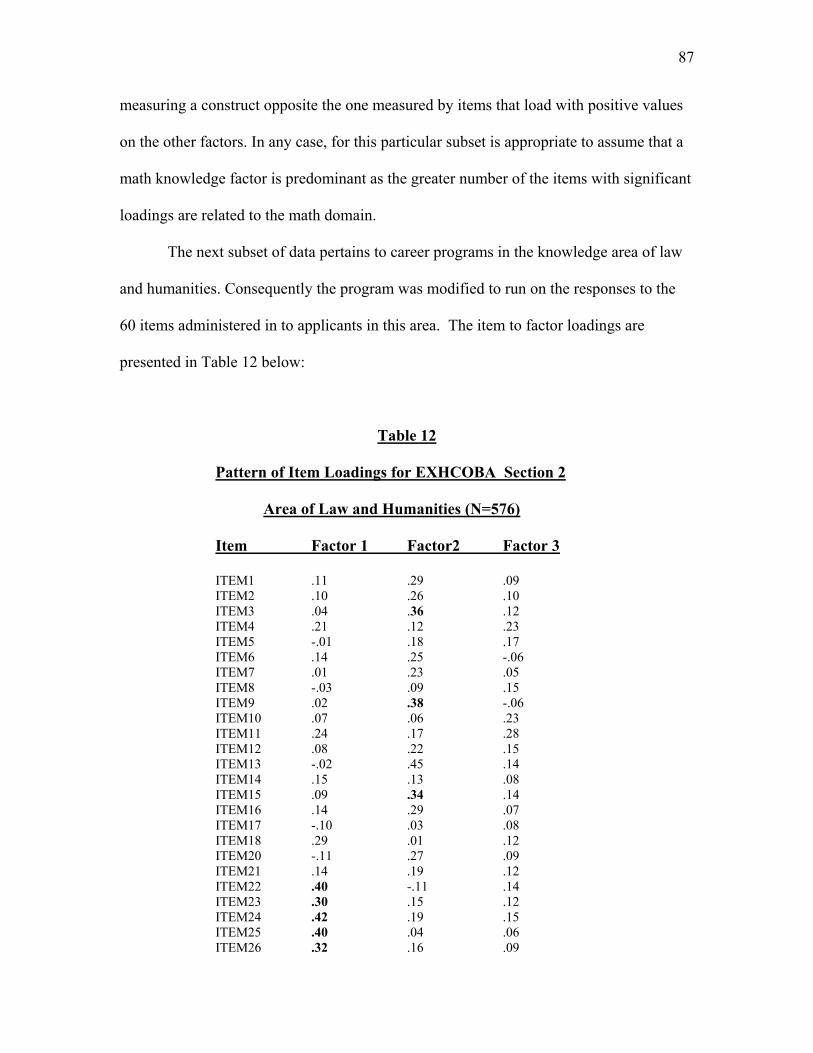
87

measuring a construct opposite the one measured by items that load with positive values

on the other factors. In any case, for this particular subset is appropriate to assume that a

math knowledge factor is predominant as the greater number of the items with significant

loadings are related to the math domain.

The next subset of data pertains to career programs in the knowledge area of law

and humanities. Consequently the program was modified to run on the responses to the

60 items administered in to applicants in this area. The item to factor loadings are

presented in Table 12 below:

Table 12


Area of Law and Humanities (N=576)


ITEM1 .11 .29 .09 ITEM2 .10 .26 .10 ITEM3 .04 .36 .12 ITEM4 .21 .12 .23 ITEM5 -.01 .18 .17 ITEM6 .14 .25 -.06 ITEM7 .01 .23 .05 ITEM8 -.03 .09 .15 ITEM9 .02 .38 -.06 ITEM10 .07 .06 .23 ITEM11 .24 .17 .28 ITEM12 .08 .22 .15 ITEM13 -.02 .45 .14 ITEM14 .15 .13 .08 ITEM15 .09 .34 .14 ITEM16 .14 .29 .07 ITEM17 -.10 .03 .08 ITEM18 .29 .01 .12 ITEM20 -.11 .27 .09 ITEM21 .14 .19 .12 ITEM22 .40 -.11 .14 ITEM23 .30 .15 .12 ITEM24 .42 .19 .15 ITEM25 .40 .04 .06 ITEM26 .32 .16 .09

88

ITEM27 .35 .03 .18 ITEM28 .40 .10 .06 ITEM29 .23 .36 .17 ITEM30 .05 .32 .04 ITEM31 .44 .16 -.05 ITEM32 .13 .30 .04 ITEM33 .35 .08 .16 ITEM33 .14 .39 -.03 ITEM34 .43 .22 -.03 ITEM35 .29 .03 .09 ITEM36 .44 .11 .16 ITEM37 .13 .03 .23 ITEM38 .41 .06 .09 ITEM39 .36 .19 .08 ITEM40 .07 .15 .10 ITEM41 .07 .30 .11 ITEM42 .14 .07 .27 ITEM43 .22 .33 .10 ITEM44 .09 .34 .12 ITEM45 .16 .16 .27 ITEM46 .19 .24 .16 ITEM47 .28 .01 .11 ITEM48 -.04 .15 .40 ITEM49 .12 .09 .35 ITEM50 .12 .05 .47 ITEM51 .20 .05 .02 ITEM52 .09 .32 .12 ITEM53 .22 .10 .09 ITEM54 .22 .24 .08 ITEM55 .27 .32 .04 ITEM56 -.01 .26 .19 ITEM57 .14 .27 .22 ITEM58 .24 .16 .11 ITEM59 .19 .13 .25 ITEM60 .15 .06 .46

The pattern of loadings above does not give a clear indication of three subscales

being measured by the 60 items. The only consistency in these item sets appears in item s

22 through 49 which are originally designed to measure knowledge of the social science

domain in the applicants to the Law and Humanities career programs. The rest of the item

loadings do not conform to the expected sub scale arrangement in the original design of

the instrument.

89

The next and final program run of the EFA procedure is done on the test data

from applicants to career programs on the Social Science area. The results are shown in

Table 13 below:

Table 13


Area of Sociology and Psychology (N=625)


ITEM1 .24 .38 -.02 ITEM2 .09 .45 .09 ITEM3 -.01 .46 .12 ITEM4 .07 .28 -.08 ITEM5 .11 .42 .14 ITEM6 .12 .31 .01 ITEM7 .08 .46 .11 ITEM8 . 17 .43 -.04 ITEM9 .01 .45 .06 ITEM10 .04 .40 .04 ITEM11 .27 .24 .03 ITEM12 .11 .44 -.08 ITEM13 .06 .34 .20 ITEM14 .12 .39 .19 ITEM15 .09 .46 .10 ITEM16 .04 .41 .05 ITEM17 .15 .33 .07 ITEM18 .26 .39 .11 ITEM20 -.05 .17 .17 ITEM21 .31 .27 .07 ITEM22 .07 .09 .34 ITEM23 .21 .08 .32 ITEM24 .08 .08 .34 ITEM25 .36 .10 .05 ITEM26 .13 .13 .08 ITEM27 .11 -.01 .19 ITEM28 -.06 .09 .36 ITEM29 .17 .06 .08 ITEM30 .06 .04 .35 ITEM31 .21 .12 .17 ITEM32 .31 .14 .25 ITEM33 .11 .09 .22 ITEM34 .02 .03 .46 ITEM35 .21 .06 .34 ITEM36 .24 .04 .13 ITEM37 -.11 -.04 .19 ITEM38 .28 .13 -.02 ITEM39 .07 .01 .16 ITEM40 .20 .06 .26

90

ITEM41 .43 .11 .09 ITEM42 .32 .08 .16 ITEM43 .37 .12 .25 ITEM44 .33 .23 .09 ITEM45 .26 .22 .27 ITEM46 .42 .19 .03 ITEM47 .31 .08 .27 ITEM48 .39 .11 .21 ITEM49 .05 .05 .32 ITEM50 .35 .02 .31 ITEM51 .17 .10 .30 ITEM52 .41 .07 -.04 ITEM53 .16 .13 .34 ITEM54 .36 -.02 .31 ITEM55 .28 -.05 -.03 ITEM56 .40 .10 .14 ITEM57 .12 .07 .13 ITEM58 .29 .04 .20 ITEM59 .35 .05 .18 ITEM60 .13 -.07 .18

The pattern of loadings presented gives and indication that the items sets comprise

three separate subscales. As can be seen, the majority of the first 20 items load under

factor 2. These items belong to the math-statistics domain. It is interesting to note that

in the sub sample of Economics and Administration this set of items displayed the same

loadings. (See Table 10). This result confirms at least in part the contention that the items

designed for the math-statistics domain do in fact comprise a sub scale

In the next 20 items there is a clear break in the pattern as items 22 through 35

which belong to the social science domain load together under factor 3. Although the not

all items in this sub set are consistent, the majority of them load under the same factor.

This lends partial support to the notion that the specialized knowledge of social sciences

is comprised under this limited sub scale.

The next and final set of 20 items begins with item 41. The pattern of loadings for

items 41 through 60 also exhibits a limited consistency as the majority of these items load

together under factor 1. This is again an indication that at least in part; this item set which

91

originally belongs to the Humanities domain does comprise a separate sub scale in this

sub sample of applicants.

The overall results of the EFA program applications uncover consistencies as well

as discrepancies of the original design of the EXHCOBA sub-scales and the obtained

patterns of loadings. Although the originally intended factor structure appears to hold,

there are number items that do not load on any of the extracted factors. For this reason,

the non-loading items are suspect of misfit. The item properties of both fitting and non-

fitting items are examined under the IRT application results.

Results of the Confirmatory Factor Analysis

As noted in the Method Section (Ch. 3), the TESTFACT 4 program includes a

special procedure for applying a distinct form of confirmatory item factor analysis under

the BIFACTOR command. The technique under this computing implementation is a type

of confirmatory factor analysis because it tests a factor pattern in which there is a general

factor on which all items have some loading, plus a number of item group factors to

which non-overlapping subsets of items are assumed to belong (SSI, 2003, p. 410).This

procedure is employed for hypothesis testing following the general form described

below:

H0 : The n items in the test section are indicators of a general factor, and the

subsets of items i to n are indicators of k uncorrelated item group factors.

H1:The n items in the test section are indicators of a general factor, and the subsets

of items i to n are indicators of k+1 uncorrelated item group factors.

92

As these hypotheses test for different item groupings, the program is run to

attempt to confirm the item groupings postulated by the theoretical structure of the

instrument with data from the randomly selected cross validation sample (N= 3054).

Therefore the first program run is applied to the first 60 EXHCOBA items

hypothesizing one general factor and two uncorrelated group factors against the

alternative that the item sets are indicators on one general factor and of three uncorrelated

item group factors.

Under the hypothesis of one general factor an item group factor the obtained χ2 =

162, 955.93, DF= 2933. The alternative hypothesis of one general factor and two

uncorrelated group factors yielded a χ2 = 162,421.00, DF= 2895.

Given the above:

162,955.93 − 162,421.00 = 534.93 with 2933-2895 = 38 DF,

the result allows for the rejection of the hypothesis of one general factor and two

uncorrelated group factors. Therefore, the hypothesis of one general factor and three

uncorrelated item group factors holds. Since the critical value for χ2 (38) = 61.162 at α =

.01 level; the value obtained in this result is 534.93 which effectively confirms the

theoretical model.

The program’s output indicates that the general factor accounts for 23.66% of the

variance while the three item group factors account respectively for 2.56, .76% and, .58

% of the variance. The remaining 72.42% of the variance is labeled as uniqueness. This

final result applies to the 2 subscales contained in the first 60 EXHCOBA items.

93

The confirmed model matches at least in part the expected model as intended in the

instrument’s original design (See Figure 6). As noted before the programming

specifications for the CFA procedures are presented in Appendix II.

The CFA procedure with the BIFACTOR command is applied to the remaining

EXHCOBA subscales following the logic outlined above.

For the next subscale comprised of 35 items measuring basic knowledge of

Spanish and math, the EFA finding indicated the presence of a general basic knowledge

factor with two item group factors. Therefore this hypothesis is tested against the null

hypothesis that p that there are one general factor and one item group factor

Under the null hypothesis the obtained test value is χ2 = 79,081.17, DF= 2983.

The alternative hypothesis of one general factor and two item group factors resulted in χ2

= 79,030.30, DF= 2971. The difference is then: 79,081.17 − 79,030.30 = 50.87 with

2983-2971 = 12 DF. Since the critical value for χ2(12) = 26.217 at the α = .01 level, the

difference of 50.87 allows the rejection of the null hypothesis. This in turn supports the

conclusion that a model with one general factor and two item group factors accounts for

the structure of this part of the instrument. The program’s output shows that in this

model the general factor accounts for 23.81% of the variance while the two item group

factors account for 1.38% and .48% respectively. The uniqueness component is 74.32%

of the variance.

The next application of the procedure runs of data from the 35 items

corresponding to basic knowledge of natural sciences and social sciences. In this case,

the null hypothesis postulates one general factor and one item group factor. The

alternative hypothesis postulates one general factor and two item group factors. Under the

94

null hypothesis the obtained test value is χ2 = 77, 299.83, DF = 2983. The alternative

hypothesis resulted in χ2 = 79, 017.59, DF = 2971. In this case the χ2 difference is in

favor of retaining the null concluding that one general factor and one item group factor

account for the structure of the test in this part of the instrument. This result is not

surprising since the exploratory analysis results gave a strong indication that the item

responses appear to be subsumed under one general factor of basic knowledge of science.

As noted before, it is likely that the item responses are not actually distinguishing

knowledge of two separate science fields and therefore the items only load on a general

knowledge factor. The output indicates that the general factor accounts for 20.10 % of

the variance while 79.90% is uniqueness in the data structure. It must be noted that this

section of the instrument yields the weakest results both in the exploratory and in the

confirmatory analyses. For this reason, the item construction and arrangement of this

section requires further examination and possibly a re-formulation of item content. This

aspect can be diagnosed better under the item fit analysis of the IRT model yet to be

reported later.

The results of the confirmatory procedures applied to section 2 of the examination

are presented next. As in the case of the exploratory part, the results that follow are taken

from the data on the specialized knowledge areas of: Business-Administration, Science-

Engineering, Law-Humanities, and Psychology-Sociology. It must be recalled that these

data sub sets met the minimum sample size requirements to be analyzed both in the

exploratory and confirmatory phases.

The CFA analysis applied to the Business- Administration sub sample ( N=562)

gives the following results. Under the null hypothesis of one general factor and two

95

uncorrelated item group factors, the obtained test value is χ2 = 34,545.32, DF= 441. The

value obtained under the alternative hypothesis of one general factor and three

uncorrelated item group factors is χ2 = 34,318.69, DF= 411.

The difference of χ2 values is 226.72 with 30 degrees of freedom. The critical

value of χ2 (30) =50.892 at the α =.01 level; therefore this result warrants the rejection of

the null and the conclusion that the data fit a model of one general factor and three

uncorrelated item group factors. This conclusion confirms again the factor structure

postulated in the theoretical model.

The proportion of variance accounted for by the factors is: 15.33% for the general

factor, 1.44% for factor 1, 5.51% for factor 2, and 1.29% for factor 3. The uniqueness for

this sub set of the data is 76.41%.

The CFA analysis applied to the Science Engineering sub sample ( N=552) gives

the following results. Under the null hypothesis of one general factor and two



uncorrelated item group factors is χ2 = 35,371.96 DF= 393.


value of χ2 (31) =52.191 at the α = .01 level, therefore this result warrants the rejection of



expected under the theoretical model.

96


factor, 4.15% for factor 1, 1.00% for factor 2, and .72% for factor 3. The uniqueness for


The CFA analysis applied to the Law and Humanities sub sample ( N=567) gives

the following results. Under the null hypothesis of one general factor and two



uncorrelated item group factors is χ2 = 35,612.44, DF= 427.


value of χ2 (29) =49.588 at the α = .01 level, therefore this result warrants the rejection of



expected.




Finally for this phase, the CFA analysis applied to the Psychology and Sociology

sub sample (N=625), gives the following results. Under the null hypothesis of one

general factor and two uncorrelated item group factors, the obtained test value is

χ2 = 36, 583.00, DF= 498. The value obtained under the alternative hypothesis of one

general factor and three uncorrelated item group factors is χ2 = 36, 177.31, DF= 466.


value of χ2(32) =53.486 at the α = .01 level, therefore this result warrants the rejection of

97



expected.




Given the results above this section concludes with the assertion that the results of

the CFA analysis on the cross validation sample support the results obtained under the

EFA procedures. However, it must be noted that the proportions of variance accounted

for by the factors identified are for the most part small with the uniqueness component

attached to the largest proportion of variance in the data sub sets. These results although

troubling are not surprising. It must be recalled that the overall applicants’ performance

on the sub-tests tends to be low in the percentage of items with correct responses. (see

Table 4). The low average performance by sub test observed in the 2003 and 2004

cohorts forecasts the general result of the factors identified by EFA and confirmed by

CFA accounting for smaller proportions of systematic variance in the 2004 EXHCOBA

data sets.

Results of the Rasch Model Application

The final task in this project was to investigate the item properties of each of the

EXHCOBA subscales by applying the Rasch Model to the data from the third randomly

drawn sub sample of the 2004 cohort (N= 3091).

98

As explained in the methods section the purpose of this part of the methodology is

to obtain item calibrations and an overall picture of how the items map in the applicants’

cognitive set of abilities as observed in the cohort.

Since the Rasch Model assumes that a set must be of one-dimension each

EXHCOBA section is examined separately to determine the properties of the

corresponding subsubscale and in particular to check for unidimensionality of the item

subset. The first set of 30 items belongs to Basic Language Ability and the results of

applying the model to them are displayed in Table 14.

Table 14

Item Calibrations for EXHCOBA Items 1 – 30: Basic Language Ability

ITEM LOGIT ERROR INFIT MSQ

INFIT ZSTD

OUTFIT MSQ

OUTFIT ZSTD CORR DISCR

1 0.75 0.04 0.99 -0.58 1.01 0.80 0.35 1.03 2 1.56 0.04 1.06 3.16 1.07 2.65 0.25 0.88 3 0.40 0.04 1.01 0.88 1.01 0.57 0.33 0.96 4 0.97 0.04 1.01 0.73 1.01 0.33 0.33 0.97 5 -1.19 0.05 0.95 -1.70 0.84 -3.67 0.35 1.07 6 -0.84 0.05 0.92 -3.59 0.84 -4.62 0.40 1.14 7 0.01 0.04 1.09 6.24 1.12 5.69 0.22 0.69 8 -0.77 0.04 1.00 0.00 0.99 -0.36 0.30 1.00 9 0.32 0.04 1.01 0.90 1.01 0.32 0.33 0.96

10 0.42 0.04 1.04 2.96 1.05 2.75 0.30 0.83 11 0.22 0.04 1.05 3.99 1.07 3.72 0.28 0.79 12 0.47 0.04 0.93 -5.99 0.92 -5.16 0.43 1.31 13 -0.48 0.04 1.02 0.99 1.04 1.34 0.29 0.95 14 0.20 0.04 0.91 -6.90 0.89 -6.55 0.44 1.35 15 0.92 0.04 1.09 6.62 1.12 6.52 0.23 0.64 16 -1.33 0.05 0.94 -1.83 0.87 -2.77 0.34 1.07 17 0.65 0.04 1.04 3.35 1.05 2.83 0.30 0.82 18 -0.18 0.04 1.00 0.25 1.00 0.22 0.32 0.99 19 -1.49 0.05 0.99 -0.24 0.96 -0.80 0.26 1.01 20 -0.84 0.05 0.96 -1.61 0.93 -2.08 0.34 1.06 21 -0.75 0.04 0.97 -1.44 0.92 -2.57 0.34 1.06 22 -0.06 0.04 1.01 0.52 1.00 0.11 0.32 0.98 23 0.56 0.04 1.03 2.12 1.02 1.35 0.32 0.89 24 -0.28 0.04 0.87 -8.37 0.81 -8.47 0.49 1.35 25 -0.41 0.04 1.02 1.08 1.01 0.22 0.30 0.96 26 -0.08 0.04 0.99 -0.55 0.98 -0.84 0.34 1.03 27 0.73 0.04 1.02 1.56 1.02 1.31 0.32 0.92

99

28 0.46 0.04 0.99 -0.98 0.98 -1.22 0.36 1.06 29 -0.61 0.04 1.01 0.32 1.00 0.13 0.30 0.99 30 0.65 0.04 1.08 6.55 1.11 6.52 0.24 0.63

As can be noted all 30 items in the basic language ability scale have values within

the logit range of -2 to +2, with the majority centering around the mean of 0 logit

difficulty. The highest logit value is 1.75 for item 2 and the lowest logit is -.06 for item

22. Also it can be noted that the error values for this estimate are relatively small

between 0.04 and 0.05.

Inspection of Table 15 with values in bold shows items: 2, 5, 6, 7, 10, 11, 12, 14,

15, 17, 23, 24, and 30, as definite misfits both in INFIT and OUTFIT. It is also

interesting to note that these items showed no significant loading on any of the factors

extracted in the EFA analysis (see Table 6). All of their values are outside the acceptable

ranges of 1 to 1.3 (unstandardized) or -2 to +2 (standardized). The interpretation for the

values is based on the standard Rasch modeling criteria presented in Chapter 3. For

reference, the values for assessing model fit are reproduced next.

For INFIT - which is a measure sensitive to responses near the person’s ability

level - the mean square infit statistic (MSQ) has an expectation of 1. Values substantially

below 1 indicate dependency in the observed data, while values substantially above 1

indicate noise. A MNSQ of 1.0 indicates perfect fit. A value of 1.3 indicates the

measure is suspect of misfit. Values above the 1.3 threshold are definite misfits indicating

noise or error in the data. Values less than 1.0 also are suspect of misfit because they

appear to fit to well. The rationale behind these limits in the statistic values is that an

INFIT mean square value of 1 + x indicates 100x% more variation between the observed

and the model-predicted response patterns that would be if the data and the model were

100

fully compatible. Therefore an INFIT value of more than 1.30 indicates 30% more

variation in the observed data than the model predicts. In the same manner, values less

than 1 indicate a given percentage of less variation in the observed data than expected by

the model,( Bond & Fox, 2001, p.177).

In INFIT the standardized values appear as INFIT ZSTD. This statistic is reported

in natural logarithms and ideally should take on values between -2 and +2. Values greater

than +2 are suspect of misfit and values less than -2 also are misfits.

The unstandardized values for INFIT and OUTFIT are reported as mean squares

and these are the mean square residual values for each item. These residual values

represent the differences between the Rasch Model’s theoretical expectation and the

performance observed for each item. It is useful to recall that infit is a weighted statistic

more sensitive to person responses that are closer to their ability level as expected by the

model. By contrast the outfit statistic is unweighted and it is more sensitive to outliers,

that is, persons responding to items that are outside their ability level by the model’s

expectation.

For OUTFIT - which is a measure sensitive to outliers - the mean square outfit

statistic (MSQ) also has an expectation of 1.0. Values substantially less than 1 indicate

dependency in the observed data; while values substantially greater than 1 indicate the

presence of outliers. A MNSQ of 1.0 indicates perfect fit. A value of 1.3 indicates the

measure is suspect of misfit. Values above the 1.3 threshold are definite misfits indicating

noise or error in the data. Values less than 1.0 also are suspect of misfit because they

appear to fit too well. The rationale behind these values is that an OUTFIT mean square

value of 1 + x indicates 100x% more variation between the observed and the model-

101

predicted response patterns that would be if the data and the model were fully

compatible. Therefore an OUTFIT value of more than 1.30 indicates 30% more variation

in the observed data than the model predicts. In the same manner, values less than 1

indicate a given percentage of less variation in the observed data than expected by the

model.

In OUTFIT the standardized values also appear as OUFIT ZSTD. For this statistic

values between -2 and +2 are within an acceptable logit range for both persons and items.

Values greater than +2 are suspect of misfit and values less than -2 also are misfits.

In the basic language ability subscale the items with definite misfit (2, 5, 6,7, 10,

11, 12, 14, 15,17,23, 24, and 30 are exceeding the limits of the criteria outlined above

and should be examined in content and construction to identify possible item design

flaws.

The second to last column of Table 15 indicate the correlation of each item with

the total score for that item (CORR). When the items are measuring the same construct

these values typically range from .25 to .75. Most of the items in this subset meet this

general rule. This is an overall indication of unidimensionality. The lower correlations do

correspond to those items that show a greater tendency towards misfit.

The last column of the table shows the item discrimination index for each item

(DISCR). This index is an estimation of how well the item distinguishes the response

patterns of persons of lower and higher ability. The standard interpretation is that the

higher discrimination values represent a better ability discrimination power for the item

in question relative to the other items in the subset.

102

It is also useful to examine the map of items and persons which shows the relative

location of each of the items to examinees. The items and persons are placed along the

scale in an order corresponding to measured item difficulty and person ability. This map

is reproduced from the program’s output in the next page. Inspection of the alignment of

persons and items shows that item 2 was the most difficult (within acceptable range) but

that a fair number of persons abilities exceeded this level of difficulty. Conversely item

19 is the easiest and very few persons are mapped below this level. Also the spread of

items from 2 to 19 shows evidence of their placement along the unidimensional scale

with some items aligned along the same difficulty score.

103

Figure 10

Map of Persons to Items from EXCHOBA Items: 1-30 Language

INPUT: 3091 PERSONS, 30 ITEMS MEASURED: 3091 PERSONS, 30 ITEMS, 2 CATS 3.37 -------------------------------------------------------------------------------- PERSONS MAP OF ITEMS <more>|<rare> 4 . + . | | | | 3 + . | | | .## | | T| 2 .### + | ##### | .####### | V2 |T .######## S| .######### | 1 .########### + V4 | V15 .########### |S V1 V17 V27 V30 .########### M| V23 .############ | V10 V12 V28 V3 .########### | V11 V9 .########## | V14 0 .######## +M V22 V7 ######## | V18 V26 .####### S| V24 .#### | V13 V25 #### | V29 .## |S V21 V8 | V20 V6 -1 .## T+ . | V5 . | V16 |T V19 . | . | | -2 . + | | . | | | | -3 + | | | . | | -4 + <less>|<frequ> EACH '#' IS 21, ‘.’ Is less than 21.

104

The most interesting feature of this item to person map is that a substantial

number of examinees exceed in ability level compared to the items’ difficulty level. This

is understandable if one takes into account the fact that this part of the instrument

measures language ability acquired during elementary school. Therefore, the general

ability of the examinees would be expected to match or exceed the subscale’s difficulty

level.

The next subscale is composed of 30 items designed to measure Basic Math

ability corresponding also to the elementary school curriculum. Item calibration results

are shown in Table 15.

Table 15

Item Calibrations for EXHCOBA Items 31-60: Basic Math Ability


INFIT ZSTD

OUTFIT MSQ


31 -0.02 0.04 1.05 2.81 1.05 1.48 0.43 0.89 32 -1 0.05 0.97 -1.35 0.94 -1.12 0.43 1.04 33 1.44 0.04 1.15 6.72 1.29 7.15 0.36 0.72 34 -0.5 0.04 0.95 -2.39 0.92 -2.14 0.47 1.09 35 0.93 0.04 1.12 6.46 1.23 7.29 0.39 0.72 36 -0.53 0.04 0.92 -4.22 0.94 -1.53 0.49 1.14 37 0.69 0.04 1.14 7.79 1.23 7.78 0.38 0.65 38 -2.14 0.06 0.92 -2 0.68 -3.73 0.37 1.09 39 0.38 0.04 0.93 -4.07 0.92 -3.14 0.53 1.17 40 -0.09 0.04 0.95 -2.78 0.96 -1.2 0.49 1.1 41 -0.9 0.05 0.93 -3.06 0.9 -2.13 0.46 1.1 42 -0.36 0.04 0.89 -6.09 0.84 -4.59 0.53 1.23 43 0.53 0.04 0.94 -3.87 0.92 -3.15 0.53 1.16 44 -0.04 0.04 0.85 -9.07 0.79 -7.35 0.57 1.35 45 -0.74 0.04 0.9 -5.08 0.83 -4.22 0.5 1.18 46 -0.52 0.04 1.03 1.74 1 0.1 0.42 0.94 47 0.75 0.04 0.9 -5.96 0.85 -5.64 0.56 1.24 48 0.71 0.04 1.04 2.14 1.06 2.23 0.46 0.91 49 1.95 0.05 1 0.04 1 0 0.45 1 50 -0.15 0.04 1.08 4.34 1.1 3.15 0.41 0.82 51 0.63 0.04 0.96 -2.41 0.95 -1.86 0.51 1.1 52 0.36 0.04 1.27 9.9 1.41 9.9 0.29 0.33 53 -0.25 0.04 0.98 -1.06 0.94 -1.68 0.47 1.05 54 -1.07 0.05 0.98 -1.02 0.96 -0.67 0.42 1.03 55 0.16 0.04 0.98 -0.96 0.96 -1.42 0.49 1.05

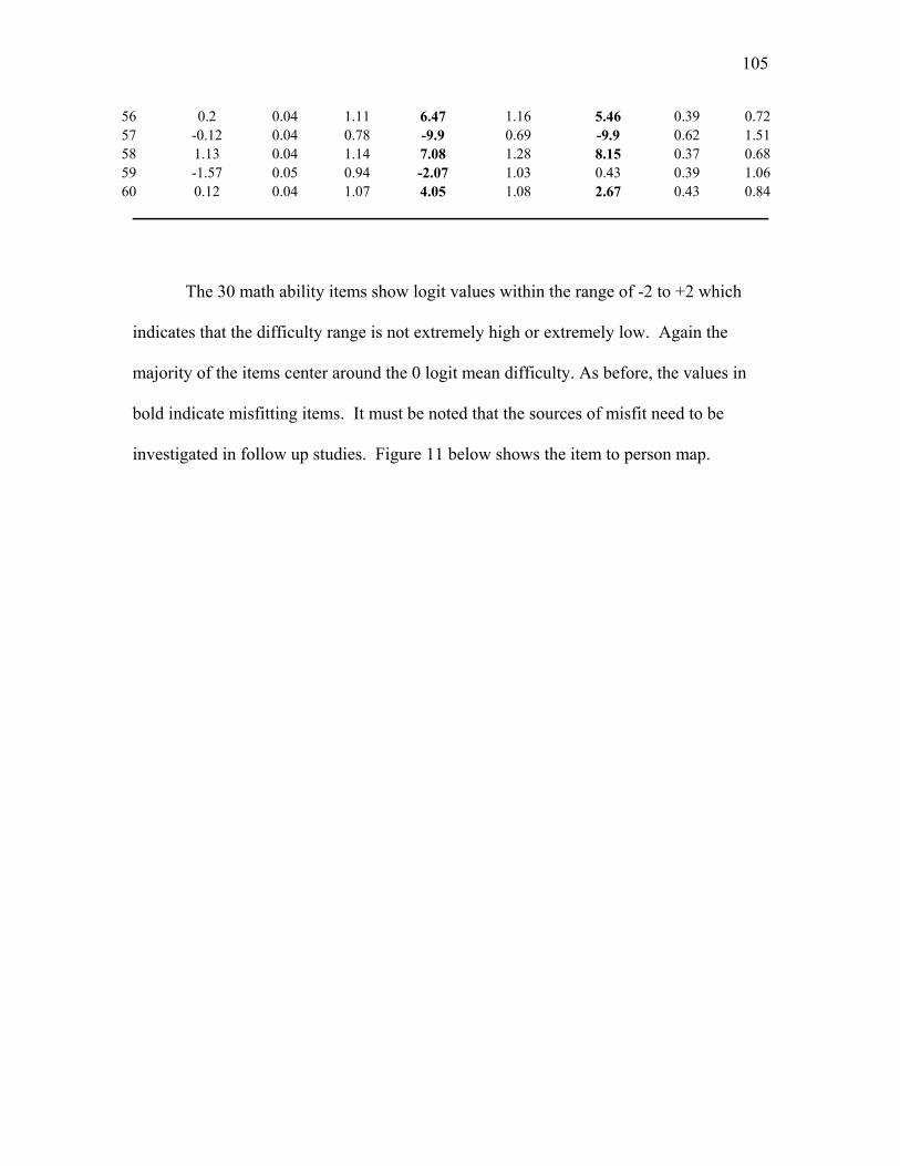
105

56 0.2 0.04 1.11 6.47 1.16 5.46 0.39 0.72 57 -0.12 0.04 0.78 -9.9 0.69 -9.9 0.62 1.51 58 1.13 0.04 1.14 7.08 1.28 8.15 0.37 0.68 59 -1.57 0.05 0.94 -2.07 1.03 0.43 0.39 1.06 60 0.12 0.04 1.07 4.05 1.08 2.67 0.43 0.84

The 30 math ability items show logit values within the range of -2 to +2 which

indicates that the difficulty range is not extremely high or extremely low. Again the

majority of the items center around the 0 logit mean difficulty. As before, the values in

bold indicate misfitting items. It must be noted that the sources of misfit need to be

investigated in follow up studies. Figure 11 below shows the item to person map.

106

Figure 11

Map of Persons to Items from EXCHOBA Items: 31-60 Mathematics

INPUT: 3091 PERSONS, 30 ITEMS MEASURED: 3091 PERSONS, 30 ITEMS, 2 CATS -------------------------------------------------------------------------------- PERSONS MAP OF ITEMS <more>|<rare> 4 .# + | .#### | | | | | 3 ###### + T| | | .####### | | .######### | 2 + V49 .########## | S|T .########### | .########## | V33 | .############ | V58 1 .############ + V35 .########## |S | V37 V47 V48 .########### | V43 V51 .############ M| V39 V52 .########## | .########### | V55 V56 V60 0 ########### +M V31 V44 .########## | V40 V50 V57 .########### | V53 .########## | V42 .######## | V34 V36 V46 | V45 .######### S|S V41 -1 .####### + V32 V54 .######## | | .####### | .#### | V59 |T .## | -2 T+ .## | V38 | . | | | | -3 . + | | | | . | | -4 + <less>|<frequ> EACH '#' IS 13.

107

The item map for subscale 2 shows that most items spread across the basic math

ability scale. This is clear by the position of the line of items from 49 to 38. Another

segment of items are placed along an equal logit difficulty measure as seen in positions

37, 47 and 48. This might be an indication of redundancy but the number of items in

these cases is not extreme compared to the spread of the rest of the items. The overall

result gives a fair indication of unidimensionality in this subscale.

It must be noted that as in the previous case the ability level of the examinees

surpassed the items’ difficulty level. This is an expected result given the basic nature of

the math ability being assessed by this section of the EXHCOBA examination.

The next section of the examination is composed of 4 separate subscales

originally designed to measure basic knowledge acquired through the exposure of

students to the secondary level curriculum (equivalent to grades 7th through 9th). These

exams’ subsection is labeled 1-B and the subscales are: (1) Basic knowledge of Spanish

(20 items), (2) Basic knowledge of math (15 items), (3) Basic knowledge of Natural

Sciences (15 items), and (4) Basic knowledge of Social Sciences (20 items).

The data from this section of the test posed the most difficult problems of analysis

and interpretation in the EFA and CFA phases, therefore the examination of item fit and

scale unidimensionality are expected to yield less interpretable results. On an added

consideration, the section on average student performance shows a sharp decrease on the

average percentage of items correct observed in the 2004 cohort (see Table 3).

108

The results from analyzing the 20 items from the basic knowledge of Spanish sub-

scale are presented in Table 16.

Table 16

Item Calibrations for EXHCOBA Items 61-80: Basic Knowledge of Spanish


INFIT ZSTD

OUTFIT MSQ


61 -0.06 0.04 1.02 1.72 1.03 1.44 0.34 0.91 62 -1.39 0.05 1.02 0.64 1.05 1.16 0.28 0.97 63 0.4 0.04 1.01 0.4 1.01 0.27 0.37 0.98 64 -0.03 0.04 1.03 2.1 1.04 1.92 0.34 0.89 65 -0.64 0.04 0.98 -1.44 0.98 -0.74 0.37 1.06 66 -2.71 0.07 0.96 -0.78 0.79 -2.49 0.27 1.04 67 0.49 0.04 1.04 3.17 1.07 3.49 0.33 0.83 68 -0.13 0.04 0.94 -4.32 0.91 -4.56 0.43 1.22 69 1.17 0.04 0.97 -1.37 1.01 0.26 0.38 1.04 70 -0.45 0.04 0.98 -1.06 0.95 -2.11 0.38 1.06 71 -0.04 0.04 1.08 5.7 1.1 5.02 0.29 0.7 72 1.63 0.05 1.05 1.96 1.23 5.67 0.27 0.9 73 -1.21 0.05 0.96 -1.75 0.92 -2.17 0.36 1.07 74 0.49 0.04 1.04 2.92 1.05 2.42 0.33 0.86 75 0.68 0.04 1.08 5.15 1.11 5.06 0.29 0.75 76 -0.04 0.04 0.96 -3.24 0.94 -3.02 0.41 1.16 77 0.15 0.04 0.93 -5.75 0.9 -5.43 0.45 1.29 78 0.8 0.04 0.93 -4.65 0.93 -3.41 0.44 1.19 79 1.05 0.04 1.01 0.47 1.05 1.76 0.35 0.97 80 -0.14 0.04 0.98 -1.53 0.97 -1.56 0.39 1.08

It is clear that items 66-69 and 70-78 have standardized OUTFIT values well

beyond the -2 to +2 range. One of the apparent reasons for misfit in this case is that these

items were answered correctly by persons who were outliers in their ability calibrations.

That is, the items were being either responded to correctly by examinees with low

calibrations in ability, or the items were being responded to incorrectly by examinees

with high calibrations in ability. These irregular or unexpected patterns of response give a

warning signal indicating that the items in question might be problematic. The sources of

difficulty can only be speculated here due to scope and space considerations. However,

109

all of these cases will be flagged and further examination of this and other subscales will

be recommended for follow up studies.

Figure 12 shows the arrangement of examinees and respondents. It is interesting

to note below that in this subscale fewer respondents score in ability logits above the

highest difficulty score in item (Item 72). Note also that item 66 is definitely below the

ability level of respondents. However, for the most part the item distribute vertically in

the difficulty scale which is a good indication of unidimensionality along the intended

construct.

110

Figure 12 Map of Persons to Items from EXCHOBA Items: 61-80 Basic Spanish

INPUT: 3091 PERSONS, 20 ITEMS MEASURED: 3091 PERSONS, 20 ITEMS, 2 CATS -------------------------------------------------------------------------------- PERSONS MAP OF ITEMS <more>|<rare> 4 . + | | | | . | | 3 + | | | .# | | | 2 .## T+ |T | .### | V72 | .###### | S| V69 1 .####### +S V79 | V78 .######### | V75 .########## | | V63 V67 V74 .############ | M| V77 0 .############ +M V61 V64 V71 V76 .############ | V68 V80 | .######### | V70 | V65 .####### S| | -1 .###### +S | V73 .### | | V62 .# T| | |T -2 . + | | | . | | V66 | -3 + | | . | | | | -4 . + <less>|<frequ> EACH '#' IS 28.

111

The next sub scale of 15 items from math gave the following results:

Table 17

Item Calibrations for EXHCOBA Items 81-95: Basic Knowledge of Math


INFIT ZSTD

OUTFIT MSQ


81 0.28 0.04 0.92 -5.06 0.92 -3.67 0.5 1.21 82 0.68 0.04 0.97 -1.65 0.98 -0.58 0.46 1.06 83 -0.52 0.04 0.95 -3.24 0.98 -0.91 0.45 1.13 84 0.96 0.04 1.04 2.11 1.09 2.52 0.4 0.92 85 0.68 0.04 1.09 4.57 1.12 4.18 0.37 0.82 86 0.65 0.04 0.89 -6.12 0.86 -5.12 0.52 1.23 87 -0.24 0.04 0.91 -6.58 0.91 -4.01 0.5 1.27 88 1.47 0.05 0.93 -2.82 0.96 -0.94 0.47 1.08 89 0.8 0.04 0.96 -2.23 0.99 -0.2 0.46 1.07 90 -0.99 0.04 0.96 -2.31 0.94 -1.74 0.42 1.09 91 -1.34 0.04 1 -0.04 1 -0.12 0.37 1 92 -1.52 0.05 0.95 -1.95 0.93 -1.54 0.39 1.06 93 -0.82 0.04 1.11 6.44 1.27 7.94 0.29 0.68 94 -0.45 0.04 1.03 2.09 1.09 3.31 0.39 0.89 95 0.38 0.04 1.18 9.9 1.26 9.9 0.29 0.52

The results for items 81, 83, 85 through 90, and 93 through 95 show very high

misfit values. In general the subscales from the section 1-B of the exam tended to show

the worst results in fit in the EFA and CFA phases of the study. The result above

corroborates the claim that the four subscales in section 1-B appear to be the most

problematic part of the EXHCOBA. These subscales showed the least regular loadings on

the extracted factors (see Tables 7 and 8). Since these subscales showed the least

consistency in the patterns of loadings, their unidimensionality is questionable and thus

the performance of the items under Rasch modeling is also suspect. The item map in

Figure 12 shows that these items have larger gaps along the difficulty scale than most

other item subsets. However, the item map shows that a small group of respondents

surpassed the most difficult items.

112

Figure 13

Map of Persons to Items from EXCHOBA Items: 81-95 Basic Math INPUT: 3091 PERSONS, 15 ITEMS MEASURED: 3091 PERSONS, 15 ITEMS, 2 CATS ----------------------------------------------------------------------- PERSONS MAP OF ITEMS <more>|<rare> 3 . + .## | | | | | .## T| 2 + | |T | .#### | | V88 | | .##### | | 1 S+ V84 |S .####### | V89 | V82 V85 V86 | .######### | | V95 | V81 .########## | | 0 M+M ############# | | V87 | | .########### | V83 V94 | | .########### | V93 |S -1 + V90 S| .######## | | V91 | | V92 .##### | | |T | -2 + .## | T| | | | | -3 . + <less>|<frequ> EACH '#' IS 32.

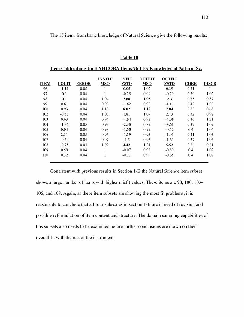
113

The 15 items from basic knowledge of Natural Science give the following results:

Table 18

Item Calibrations for EXHCOBA Items 96-110: Knowledge of Natural Sc.

ITEM LOGIT ERROR INNFIT

MSQ INFIT ZSTD

OUTFIT MSQ


96 -1.11 0.05 1 0.05 1.02 0.39 0.31 1 97 0.1 0.04 1 -0.25 0.99 -0.29 0.39 1.02 98 0.1 0.04 1.04 2.68 1.05 2.3 0.35 0.87 99 0.61 0.04 0.98 -1.62 0.98 -1.17 0.42 1.08

100 0.93 0.04 1.13 8.02 1.18 7.84 0.28 0.63 102 -0.56 0.04 1.03 1.81 1.07 2.13 0.32 0.92 103 0.63 0.04 0.94 -4.54 0.92 -4.06 0.46 1.21 104 -1.36 0.05 0.93 -2.35 0.82 -3.65 0.37 1.09 105 0.04 0.04 0.98 -1.35 0.99 -0.52 0.4 1.06 106 2.31 0.05 0.96 -1.39 0.95 -1.05 0.41 1.05 107 -0.69 0.04 0.97 -1.5 0.95 -1.61 0.37 1.06 108 -0.75 0.04 1.09 4.42 1.21 5.52 0.24 0.81 109 0.59 0.04 1 -0.07 0.98 -0.89 0.4 1.02 110 0.32 0.04 1 -0.21 0.99 -0.68 0.4 1.02

Consistent with previous results in Section 1-B the Natural Science item subset

shows a large number of items with higher misfit values. These items are 98, 100, 103-

106, and 108. Again, as these item subsets are showing the most fit problems, it is

reasonable to conclude that all four subscales in section 1-B are in need of revision and

possible reformulation of item content and structure. The domain sampling capabilities of

this subsets also needs to be examined before further conclusions are drawn on their

overall fit with the rest of the instrument.

114

Figure 14

Map of Persons to Items from EXCHOBA Items: 96-110 Knowledge of Natural Sc.

INPUT: 3091 PERSONS, 15 ITEMS MEASURED: 3091 PERSONS, 15 ITEMS, 2 CATS ----------------------------------------------------------------------- PERSONS MAP OF ITEMS <more>|<rare> 4 . + | | | | | | | 3 .## + | | | | T| | V105 .#### | 2 + |T | ####### | | S| | .######### | 1 +S | V100 .############ | | V102 V108 V99 .############ M| | V109 | .########### | V97 V98 0 +M V104 .########## | | | .####### S| V101 | | V106 V107 .#### | -1 +S | V110 V96 .## | | V103 T| .# | | |T -2 + . | | | | | | -3 . + <less>|<frequ> EACH '#' IS 35.

115

The final subscale in section 1-B of the examination contains 20 items measuring

basic knowledge of Social Sciences. The item calibration results appear below:

Table 19

Item Calibrations for EXHCOBA Items 111-130: Knowledge of Social Sc.

ITEM LOGIT ERROR INFIT MSQ INFIT ZSTD OUTFIT MSQ


111 1.15 0.04 1.09 4.25 1.17 5.01 0.28 0.82 112 0.26 0.04 0.99 -0.83 0.98 -0.85 0.4 1.04 113 0.85 0.04 0.95 -2.97 0.98 -0.62 0.43 1.1 114 0.59 0.04 1.02 1.28 1.08 3.49 0.36 0.92 115 0.78 0.04 1.01 0.42 1.02 0.77 0.38 0.98 116 -0.23 0.04 1.09 6.8 1.16 7.26 0.28 0.64 117 -0.05 0.04 0.97 -2.55 0.95 -2.61 0.42 1.14 118 0.85 0.04 0.99 -0.35 1.01 0.44 0.39 1.01 119 0.6 0.04 1.08 5.3 1.12 4.93 0.31 0.76 120 1.85 0.05 1.04 1.19 1.11 2.26 0.31 0.95 121 -0.14 0.04 0.89 -8.5 0.85 -7.61 0.49 1.41 122 0.77 0.04 0.89 -6.61 0.86 -6.06 0.49 1.27 123 -0.79 0.04 0.94 -3.78 0.93 -2.64 0.42 1.15 124 -0.77 0.04 0.92 -5.09 0.87 -4.7 0.44 1.21 125 0.31 0.04 0.96 -2.7 0.93 -3.38 0.43 1.14 126 0.4 0.04 1.11 7.53 1.13 6.15 0.28 0.64 127 -1.31 0.05 1.07 2.75 1.17 3.95 0.25 0.88 128 -2.04 0.05 0.95 -1.43 0.88 -2.1 0.33 1.05 129 -1.73 0.05 0.97 -0.96 0.97 -0.66 0.32 1.03 130 -1.34 0.05 1.01 0.55 1.1 2.35 0.31 0.97

It can be easily seen that this subscale shows the same tendency toward misfit as

the other three subscales in Section 1-B. It is not possible at this point to examine all

sources of misfit. Yet, it is reasonable to suspect that this subscale may have domain

sampling problems as the Social Sciences curriculum may well be one of the most

scattered areas in content and item construction. For this reason the recommendation of

further examination of item content, structure, and domain sampling characteristics

applies here as well as in the case of the Natural Science subscale. One interesting aspect

is that in Figure 14, items and persons matched in difficulty and ability more than any

other subscales have up to this point.

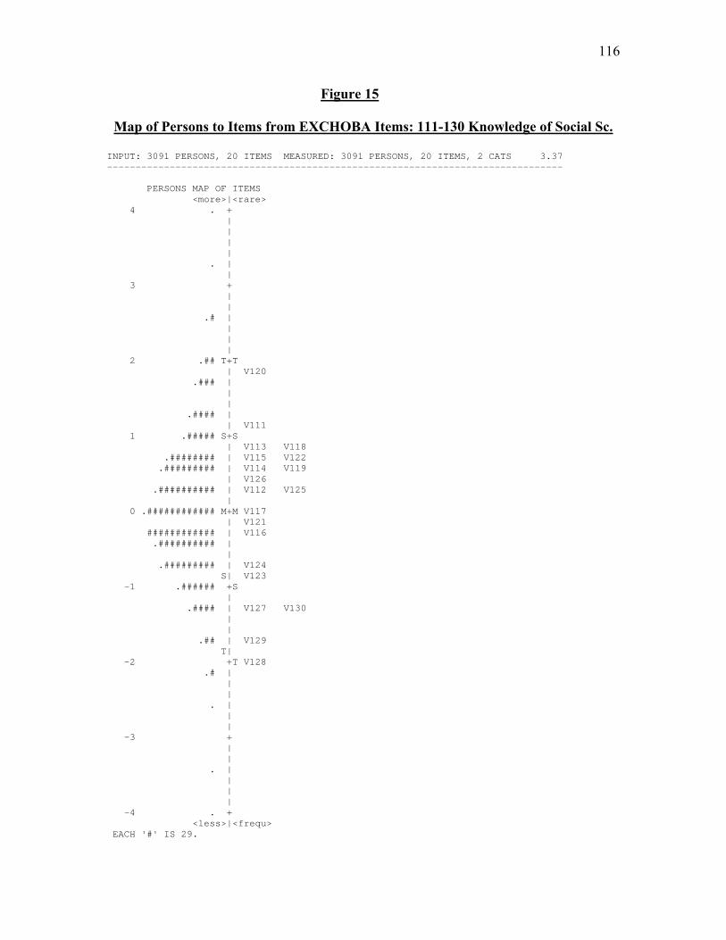
116

Figure 15

Map of Persons to Items from EXCHOBA Items: 111-130 Knowledge of Social Sc. INPUT: 3091 PERSONS, 20 ITEMS MEASURED: 3091 PERSONS, 20 ITEMS, 2 CATS 3.37 -------------------------------------------------------------------------------- PERSONS MAP OF ITEMS <more>|<rare> 4 . + | | | | . | | 3 + | | .# | | | | 2 .## T+T | V120 .### | | | .#### | | V111 1 .##### S+S | V113 V118 .######## | V115 V122 .######### | V114 V119 | V126 .########## | V112 V125 | 0 .############ M+M V117 | V121 ############ | V116 .########## | | .######### | V124 S| V123 -1 .###### +S | .#### | V127 V130 | | .## | V129 T| -2 +T V128 .# | | | . | | | -3 + | | . | | | | -4 . + <less>|<frequ> EACH '#' IS 29.

117

IRT Results by Specialized Career Area Knowledge

The EXHCOBA sub sections designed to measure specialized area knowledge are

composed of 3 subscales of 60 items each with 20 items per subscale. Recalling previous

descriptions these item subsets are administered to groups of applicants according to the

career program to which admission is attempted. For present purposes the behavior of the

items in these subsections are analyzed for the career areas of Business Administration

(N = 545) Engineering Sciences, Law - Humanities, and Sociology and Psychology, since

the data set from these areas were analyzed in the previous phases of this study.

The results of the item subscales administered to the area of Economics and

Administration are presented and discussed below. The results of the rest of the career

areas are presented in Appendix V due to space considerations.

Table 20

Item Calibrations for EXHCOBA Items 131-150 Math-Statistics


INFIT ZSTD

OUTFIT MSQ

OUFIT ZSTD CORR DISCR

131 -0.46 0.1 0.95 -1.51 0.91 -1.55 0.48 1.17 132 -0.52 0.1 0.94 -1.82 0.9 -1.86 0.49 1.21 133 0.89 0.11 0.92 -1.45 0.92 -0.81 0.47 1.11 134 0.36 0.1 1.16 3.25 1.29 3.67 0.3 0.67 135 -0.73 0.1 0.96 -1.06 0.96 -0.73 0.46 1.11 136 1.5 0.13 1.05 0.57 1.25 1.64 0.33 0.93 137 -0.68 0.1 0.95 -1.32 0.96 -0.72 0.46 1.13 138 -0.48 0.1 1 0 1 0.02 0.44 1.01 139 -0.55 0.1 0.97 -1.01 0.93 -1.32 0.47 1.13 140 1.33 0.12 1.01 0.13 0.96 -0.29 0.39 0.99 141 -0.98 0.1 0.99 -0.21 1.03 0.45 0.43 1 142 -0.12 0.1 0.95 -1.29 0.97 -0.57 0.47 1.12 143 1.48 0.13 1.03 0.43 1.12 0.82 0.35 0.95 144 -0.58 0.1 1 0.02 0.98 -0.38 0.44 1.02 145 -0.79 0.1 0.94 -1.85 0.91 -1.57 0.48 1.2 146 0.5 0.1 1 -0.09 0.99 -0.07 0.43 1 147 -0.82 0.1 1 -0.04 1.01 0.19 0.43 1 148 0 0.1 0.99 -0.2 1.02 0.39 0.44 1.01 149 1.42 0.13 1.22 2.74 1.39 2.56 0.22 0.77 150 -0.77 0.1 0.98 -0.47 0.98 -0.29 0.45 1.06

118

Table 20 shows only two items with INFIT and OUTFIT values higher that the

acceptable range of -2 to +2. As only items 134 and 149 have fit problems it must be

considered that in the EFA and CFA parts of the analysis this subscale was found to be

also one of the better fitting according to the originally design structure, (See Table 11).

The IRT result lends partial support to the claim that in general the subscales from the

specialized area knowledge show the strongest indications of unidimensionality. The item

map in figure 15 shows that most items are in the -1 to +1 range of difficulty with the

majority of the examinees aligning in this range. However, it is to be noted that even

though this is one of the subscales that performed best in previous analyses, there is a

number of respondents with ability levels well below the -1 logit range. This result in

particular can be taken as an indication that the content and performance tasks of the

items in this subscale are in fact beyond the ability level of those respondents with lower

scores. Given the statistical characteristics shown by this subscale, it is paramount to note

that the curriculum and instruction, to which the low scoring respondents were exposed,

must be traced in the different EXHCOBA versions and come under scrutiny in follow up

studies.

119

Figure 16

Map of Persons to Items from EXCHOBA Items: 131-150 Math-Statistics.

INPUT: 545 PERSONS, 20 ITEMS MEASURED: 545 PERSONS, 20 ITEMS, 2 CATS ---------------------------------------------------------------------- PERSONS MAP OF ITEMS <more>|<rare> 4 . + | | | | . | | 3 + | | .# | | | | 2 .# + | T|T .### | | V136 V143 V149 .## | V140 | 1 .### + |S V133 .##### | S| V146 .##### | V134 | .##### | 0 .####### +M V148 | V142 .######## | M| V131 V138 ############ | V132 V139 V144 .########## | V135 V137 V150 |S V145 V147 -1 .########### + V141 | .######### | | .######### S| |T | -2 .#### + | | .#### | | T| | -3 + .# | | | | | | -4 .# + <less>|<frequ> EACH '#' IS 5.

120

Table 21

Item Calibrations for EXHCOBA Items 151-170 Social Sciences


INFIT ZSTD

OUTFIT MS


151 -0.23 0.09 0.98 -0.62 1 0.06 0.34 1.07 152 -0.18 0.09 0.98 -0.89 0.98 -0.64 0.35 1.12 153 -0.54 0.09 0.93 -2.18 0.91 -2.14 0.4 1.27 154 -1.77 0.12 0.95 -0.64 0.99 -0.13 0.38 1.05 155 -0.37 0.09 0.96 -1.45 0.96 -1.11 0.37 1.18 156 -1.01 0.1 1.06 1.25 1.1 1.62 0.27 0.88 157 0.31 0.09 0.98 -0.71 0.97 -0.83 0.33 1.1 158 0.84 0.1 1.05 1.28 1.06 1.09 0.22 0.87 159 0.72 0.1 1.03 0.66 1.03 0.58 0.27 0.94 160 1.73 0.12 1.03 0.43 1.01 0.06 0.21 0.97 161 -0.13 0.09 0.99 -0.38 0.98 -0.6 0.33 1.07 162 -0.53 0.09 1 -0.11 1.01 0.26 0.33 1.01 163 -0.65 0.09 0.92 -2.36 0.9 -2.31 0.41 1.27 164 -0.2 0.09 1.01 0.24 1 -0.1 0.32 0.99 165 0.37 0.09 0.93 -2.52 0.92 -2.07 0.38 1.3 166 0.56 0.09 1 -0.1 1 -0.08 0.3 1.01 167 0.97 0.1 1.09 1.89 1.16 2.35 0.17 0.8 168 -0.74 0.09 1.08 2.24 1.1 2 0.24 0.75 169 0.67 0.1 1 0.11 1.01 0.22 0.29 0.98 170 0.18 0.09 1.02 0.76 1.04 0.96 0.29 0.89

The social science subscale has five items with infit values greater than

expected. This is an indication of unexpected patterns of response observed near the

respondents ability levels. Figure 16 shows a no overall noticeable disparities between

the item set difficulty estimates and the ability levels observed in this subsample. It is fair

to speculate that these unexpected responses might represent incorrect responses to items

near or at the ability levels in respondents who might have been working in haste as this

subscale is located near the end of the examination.

121

Figure 17

Map of Persons to Items from EXCHOBA Items: 151-170 Social Sciences

INPUT: 545 PERSONS, 20 ITEMS MEASURED: 545 PERSONS, 20 ITEMS, 2 CATS ----------------------------------------------------------------------- PERSONS MAP OF ITEMS <more>|<rare> 4 + | | | | | . | | 3 + | | | | . | | | 2 + . | | V160 | . |T T| .## | | 1 .#### + V167 | V158 .##### |S V159 S| V169 .###### | V166 | V165 .######## | V157 | V170 0 ############ M+M | V152 V161 .######### | V151 V164 | V155 ########## | V153 V162 | V163 .####### S|S V168 | -1 .### + V156 | .## | | . T|T | | V154 . | -2 + | | . | | | | | -3 # + <less>|<frequ> EACH '#' IS 7.

122

Table 22

Item Calibrations for EXHCOBA Items 171-190 Economics-Administration


INFIT ZSTD

OUTFIT MS


171 -0.02 0.09 1.01 0.24 1.01 0.29 0.36 0.98 172 0.55 0.1 0.97 -0.79 0.93 -1.25 0.37 1.11 173 -0.59 0.1 1.08 2.16 1.09 1.78 0.32 0.78 174 0.76 0.1 0.99 -0.28 0.97 -0.46 0.34 1.04 175 1.07 0.1 1.1 2.01 1.24 2.87 0.21 0.8 176 -0.62 0.1 0.96 -1.19 0.97 -0.62 0.42 1.12 177 -0.24 0.09 1.1 3.26 1.13 2.91 0.28 0.61 178 -1.21 0.1 0.99 -0.17 0.99 -0.19 0.4 1.02 179 1.21 0.11 1.04 0.66 1.18 1.96 0.25 0.91 180 0.98 0.1 0.92 -1.71 0.88 -1.73 0.39 1.16 181 -0.02 0.09 0.96 -1.35 0.95 -1.23 0.4 1.18 182 0.07 0.09 0.94 -2.2 0.91 -2.18 0.42 1.28 183 0.37 0.09 0.94 -1.81 0.91 -1.9 0.41 1.22 184 0.16 0.09 0.99 -0.47 1 -0.07 0.37 1.05 185 -0.37 0.09 1.07 2.08 1.09 2.01 0.31 0.75 186 -0.52 0.09 0.92 -2.34 0.89 -2.4 0.45 1.27 187 0.02 0.09 0.95 -1.56 0.94 -1.5 0.41 1.2 188 -0.63 0.1 1.02 0.44 1.07 1.36 0.36 0.93 189 -0.63 0.1 1.03 0.82 1.01 0.28 0.36 0.94 190 -0.32 0.09 1.01 0.4 1.01 0.21 0.37 0.96

Again the higher infit values here might be an indication of the haste effect given

the mapping of item difficulties and respondents’ abilities shown in Figure 17. As can

easily bee seen all items and respondents are within acceptable ranges, although a small

number of respondents scored below in ability.

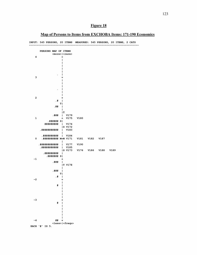
123

Figure 18

Map of Persons to Items from EXCHOBA Items: 171-190 Economics

INPUT: 545 PERSONS, 20 ITEMS MEASURED: 545 PERSONS, 20 ITEMS, 2 CATS ----------------------------------------------------------------------- PERSONS MAP OF ITEMS <more>|<rare> 4 + | | | | | . | 3 + | | | . | | | 2 + .# | T| .## | | |T .### | V179 1 + V175 V180 .###### S| ######### | V174 |S V172 .########### | V183 | .########## | V184 0 .########## M+M V171 V181 V182 V187 | .############ | V177 V190 .########### | V185 |S V173 V176 V186 V188 V189 .######### | .####### S| -1 + .### | |T V178 | .### | T| .# | -2 + | # | | | | | -3 + # | | | | | | -4 ## + <less>|<frequ> EACH '#' IS 5.

124

The remaining scales in the specialized career knowledge areas were analyzed

and the results for the most part are similar to the description of item and subscale

performance presented above. The subscales on the specialized career area knowledge of

the instrument showed for the most part equivalent results as the item maps indicate that

these subscales are targeted to the observed ability levels of the applicants in the 2004

cohort. This result is encouraging because it is also an indication that factual curriculum

as measured by the applicant’s responses is aligned with the subscales administered

according to career program choice. The item fit indices and item maps for these

subscales are presented by career knowledge area in Appendix III.

The overall results of the Rasch analysis reveal that while most subscales perform

as expected the item sets belonging to Section 1-B are the most doubtful in performance.

This finding is consistent with the EFA and CFA results. It will be recalled that items

targeted at basic knowledge of Spanish, Math, Natural Science, and Social Science

showed the least strength in factor loadings and the two common factors model was not

confirmed with respect to the 35 items targeted at basic knowledge of Natural and Social

Sciences. This particular situation is a cause of concern about the fit of the items in this

subscale with the rest of the instrument. The next and final section of this manuscript

addresses this concern and advances recommendations for further analysis of the

problematic aspects of this subscale.

Most importantly, the EXHCOBA subscales - with the exceptions noted above -

demonstrate reasonable unidimensionality under the IRT application. This finding is also

encouraging as it corroborates the structural properties found in previous analyses and

gives fair support to the instrument’s originally intended design vis a vis the Sonoran

125

high school curriculum. The investigation of unidimensionality indicates that in most

cases the subscales are constructed in a manner which affords the instrument’s expected

performance and intended use. As in all cases the item difficulty calibrations exhibit

values within acceptable ranges, it can be concluded that the irregular patterns of

response found to produce item misfit may be indications of problems during the exam

administration or of factors related to special circumstances in examinees that need to be

uncovered by studies that focalize on the actual dynamics to the test administration.

126

CHAPTER 5

REVIEW OF IMPLICATIONS AND CONCLUSIONS

This chapter reviews the results and implications for the EXHCOBA testing

practices at the Universidad de Sonora. The findings after applying the three

methodological phases of this study show reasonable consistency. While the instrument’s

subscales performed according to original design expectations, the four subscales in

Section 1-B, showed the least consistency overall. However, the concern with the

performance of the EXHCOBA subscales needs to be reviewed in the context of the

overall characteristics of the testing program as applied at the University of Sonora. The

main implications of the findings presented in Chapter 4 are discussed below. The order

of the discussion addresses first general concerns that emerge form current use of the

EXHCOBA in Sonora. The psychometric implications of the findings are then discussed

in the content of academic standards definitions. The section closes with general

conclusions and recommendations.

Discussion of General Implications

The testing system is presently serving the purpose for which it was adopted in

1997 which is to aid in the selection and placement of applicants in professional career

programs. Beyond this fact, the methodology applied to the test data has revealed

important differences in the performance of applicants. This concern has been recognized

by the academic authorities at the University of Sonora (Gonzalez & Lopez, 2004). With

the findings contained in the present study it is possible to point to specific issues that

need to be addressed.

127

First and foremost the issue of test preparation for the EXHCOBA examination

needs to be given serious consideration by academic authorities in the high school system

as a whole. The overall low performance in the subsections of the test that is consistently

observed in the 2003 and 2004 cohorts is a strong indication that the first obstacle may be

the lack of a student support system for the standardized testing requirements.

The overall average performance of applicants in all sections of the examination

barely rises above 18 correct out of 30 items in the basic language ability subscale. The

lowest performance is observed in the basic knowledge of math subscale with 6 items out

of 15 items correct. (see Table 4). In percentage terms the average for these cohorts is

60% items correct in basic language and 40% correct in basic math. The overall picture is

that in these basic areas the applicants are scoring well below a minimum proficiency

level. The traditional standard of proficiency is defined as 60 % minimum performance

for a passing grade throughout the Mexican educational system. None of the other

observed performance levels in the other subscales show substantial improvement over

these basic area skills. These performance trends have been recognized and documented

by researchers at the EXHCOBA development facility (Larrazolo, 2004) and also by

researchers at the Universidad de Sonora (Gonzalez & Lopez, 2004).

Given that the low performance is observed in areas and skills that are so basic it

is reasonable to suppose that adequate attention is not being given in current practice to

resources for basic skills review and adequate test preparation practices. The most

obvious place to begin is by enacting institutional strategies that ensure that all applicants

receive adequate preparation on the EXHCOBA format and general requirements before

graduation from their highs schools of origin. Recommendations for a strategy that

128

ensures systematic exam preparation and fair practice are presented in the conclusions

section of this manuscript.

Implications for Current Testing Practice

The statistical properties of the instrument have shown an acceptable degree of

subscale performance under a three-stage methodological framework. The exploratory

and confirmatory methods employed at the item level have produced sufficient evidence

to support limited claims of construct validity for Sections 1-A and 2 of the EXHCOBA.

Limited evidence was also found to question further the properties of the item sets that

attempt to measure basic knowledge constructs of knowledge of natural and social

sciences in Section 1-B.

The factor solutions explored and confirmed indicate that basic abilities and basic

knowledge are measured by the item subsets following distinct unidimensional structures.

However, there are also item sets that did not perform under the framework expected by

subscale design. The item sets that did not load on any of the extracted factors are listed

by subscale below:

Basic Language Ability (Subscale 1) Items: 2, 3, 7, 9, 10, 11, 13, 15, 16, 17, 18, 19, 20,

23, 25, 25, 27, 28, 29, and 30.

Basic Math Ability (Subscale 2) Item: 52.

Basic Knowledge of Spanish (Subscale 3) Items: 62, 63, 65, and 71 through 80.

Basic Knowledge of Math (Subscale 4) Items: 81 through 85, 89, 90, and 93.

Basic Knowledge of Natural Sciences (Subscale 5) Items: 97, 98, and 101 through 110.

129

Basic Knowledge of Social Sciences (Subscale 6) Items: 111 through 113, 115 through

120, 125, 127, and 128.

For those item sets that do load on the extracted factors it must be taken into

consideration that the confirmed factors accounted for very modest proportions of

variance in the data sets. This is a clear indication that the variability in the data sets that

represent applicants’ academic performance is stemming from sources not being directly

detected by the examination. These sources need to be hypothesized, tested, and

explained in follow up studies. Further application of the methods employed in this

dissertation can be profitably used to examine differences between selected sections of

the high school system. Particularly, a study employing the three-stage methodology can

be conducted with a focus on the test performance of students that are about to exit the

state high school system. The item subsets listed above need to be reviewed to locate at

least initially if the source of the problems lies in the content or construction

characteristics of the items or on the particularities of curriculum and implementation in

high schools.

The item review can be accomplished by comparing the item tasks to selected

parts of the curriculum to find at least fair indications of conceptual correspondence. The

same implication holds for selected items in the specialized knowledge subscales by

career area. This aspect of the technical properties of the items can profitably be

investigated by adapting a method of alignment studies as the one proposed by Webb

(1999), as a follow up to the present study. Follow up studies on alignment need to be

implemented as a concerted effort between the test developer and curricular design

offices of the high school system. The study of alignment of curricular content with the

130

subsections of the exam that have shown areas of concern is presented as a general

recommendation in the concluding section of this manuscript.

However, the study of the alignment of EXHCOBA and the Sonoran High School

official curriculum must follow a concerted effort to apply the fair and professionally

testing preparation practices at the high school level. The reason that such strategy must

be implemented first is that the curricular content and the examination in place may have

a high degree of conceptual correspondence, but this possibility is likely to be obscured

by the lack of an adequate system of academic review and test preparation for students at

the high school level.

Implications for Academic Standard Setting

The original intent of this study is addressed in light of the main findings as with

the following lines of argument:

(a) EXHCOBA, as a large-scale comprehensive examination for selection and

placement of applicants to university career programs, embodies a set of

content standards defined by the technical properties of the nine subscales.

(b) The University of Sonora has adopted these content standards in a general

form at least implicitly by the continued use of the EXHCOBA testing system.

Based on the analysis of current practice, the academic authorities of the

institution are in the position to define specific performance standards for the

academic process of each professional career program on the basis of the

EXHCOBA system implementation.

131

(c) The statistical methodology employed in this dissertation offers a preliminary

but adequate picture of the type of results that can be expected by continuing

current trends. While future results cannot be judged as adequate or

inadequate a priori, the trends observed and reported in this study merit the

design and implementation of strategies of academic standards setting for

professional studies at the University of Sonora.

(d) An explicit definition of basic academic standards for each of the existing

career programs begins with a large-scale statistical analysis or data derived

from current educational practice. The results obtained serve as a definite

baseline against which future results can be compared. A comparative process

allows defining, on the basis of sound measurement instruments, the academic

standards that are being met de facto by applicants. The processes will

likewise reveal grey areas where the data analysis suggests that the academic

standards are not being adequately met. Consequently, these areas are to be

targeted for improvement at the levels of curricular design and instructional

implementation.

(e) Given the fact that at present no minimum performance standard has been

defined either for the total score or for the separate subscales of the

instrument, the applicants have continued to score in the lower end of the

EXHCOBA scale. The descriptive statistics and the statistical analysis

presented in this study have given an adequate representation of the lower

limits on EXHCOBA performances and the overall inconsistencies on

performance by subscale.

132

Following the argumentation above leads to the proposal or three lines of action:

(1) The design and implementation of a test preparation program at the

high school level,

(2) The definition of expected performance standards by career program at

the university level, and

(3) The design and implementation of alignment studies to match the

Academic Standards defined with the assessment instrument in place.

The lines of action above are proposed and justified as a result of the

appraisal of current practice and based on the statistical analysis results produced

in this study. The general content of each proposal is presented below.

Design and Implementation of a Test Preparation Program

The EXHCOBA examination system has a student preparation system available

for applicants in Sonora. This system consists of an electronic guide to the examination

which is available in floppy disk format and also online at the test developer’s website. In

the past, the University of Sonora has recommended that applicants review the

EXHCOBA guide and take the practice exam. Yet, this has been left up to the individual

applicant’s discretion and has not been set forth as an official requirement.

The situation described can change and progress toward substantial improvement

in applicants’ performance if a simple and systematic process is enacted at the high

school level.

Namely, the academic orientation or school counseling programs in place at the

High School level can be modified to include a test preparation program based on the

EXHCOBA format and general requirements. It is perfectly feasible that at the beginning

133

of the senior year (5th high school semester in Sonora), all students be inducted into a

two phase test preparation program as outlined below:

A) Phase I would consist of an individual self-assessment of academic

performance. This would be a systematic exercise where each senior

examines her or his own academic strengths and areas in need of

improvement with the aid of a academic assessment survey to be

developed ex-profeso.

B) Phase II would consist of the actual EXHCOBA Practice Exam adapted

to give students individual results by each of the nine subscales. The

student individual results can then be compared with the data obtained

from the Individual Self-assessment of Academic Performance. This

comparative exercise in turn would enable the student and the academic

counselor to target areas of concern to be worked on before the actual

EXHCOBA examination takes place.

The program outlined above can be designed and conducted at the school

counseling level by effectively joining the academic student-planning domain with the

individual career planning concerns of the high school seniors approaching completion of

their high school program of studies. The key to this approach is the requirement of a

systematic self- examination and student preparation that would place students on a

trajectory of improved performance in the EXHCOBA. The added advantage to this

approach is that the students would also have an early opportunity to preview the actual

standardized testing process and to realize the performance expectations upheld by the

University of Sonora.

134

Definition of Performance Standards Expected at the University Level

The University of Sonora is an institution created by an act of State legislation

approved in 1942 and revised in 1991. The current legal framework empowers the

institution to design and implement professional career programs and to grant degrees

upon completion of the requirements of the approved programs of study. Given the fact

that the university is legally empowered to set academics requirements, it follows that the

institution can set academic standards for admission and completion of the prescribed

programs of study. It is then reasonable to propose that the academic authorities adopt

performance standards that are both necessary and sufficient for promoting a systematic

improvement of the academic processes at the student level. The establishment of

adequate levels of academic proficiency is a complex decision making process that has

been examined and documented professionally (Cizek, 2001).

A systematic effort aimed at determining sufficient performance levels for each

career program at the University of Sonora can take as a departure point the traditionally

adopted 60% level of performance to operationalize the basic level of student

proficiency. This decision and its implications can be explored at the level of each

individual career program either by assigning a 60% performance level to each of the

subscales or else to the total EXHCOBA score expected. The customary labels of Basic,

Proficient and Advanced can then be defined based on the current minimum of 60%. A

simple but effective starting point based on items correct is: 60% to 69% for the Basic

level, 70% to 79 % for the Proficient level, and 80% and above for the Advanced level.

While the scheme just described is not new, it is defensible to suppose that it is implicitly

135

applied in most judgments of academic performance. The idea here is to employ the

scheme as a starting point to then proceed to set realistic performance goals for

graduating high school seniors and university program applicants. In principle the use of

EXHCOBA and the psychometric properties of the instrument are a sound basis for this

decision making process.

Design and Implementation of Alignment Studies

The high school system in Sonora periodically modifies its official curricular

design and instructional implementation procedures. For example, the largest state high

school institution, Colegio de Bachilleres de Sonora (COBACH), has recently modified

all curricular content standards (Direccion Academica COBACH, 2004). The

implementation of institutional curricular re-design programs would be most profitable

when enacted in line with the framework of evaluating student performance with

standardized instruments as the EXHCOBA examination. The results of the statistical

analysis sections of this study are already a basis to begin the design of alignment studies

at this level. Alignment is defined as a property of the relationship between a set of

curricular content standards and the psychometric scales employed to assess the actual

student performance expected from academic content standards (Webb, 1999). The

present situation in Sonora requires that at least pilot alignment studies be conducted

since the use of standardized testing instruments to assess students is a reality in the state

since 1997.

136

The design and conduction of this type of studies can be implemented by a joint

task force composed academic experts from the Universidad de Sonora and the Colegio

de Bachilleres de Sonora.

Recommendations

Academic authorities at the University of Sonora and High School COBACH

level can begin to consider the enactment of the lines of action outlined in the previous

section. In particular, the design and implementation of an EXHCOBA test preparation

program at the high school level is at this point essential. The consistently observed low

levels of performance are sufficiently known, therefore, systematic programs to

remediate the baseline observed levels of student performance should be made a priority.

The design of a program for a school counseling intervention that addresses

adequate test preparation and students’ self appraisal of academic performance can be

planned during the spring of 2005. A piloting application of the program could then

follow for implementation with a sample from the senior class of 2005 during the fall

semester. After piloting and adjustments are complete the Test Preparation Program

would be ready for statewide implementation by the fall 2006 semester.

The program outlined above needs to be considered first by the academic

authorities of the Colegio de Bachilleres de Sonora as this institution represents the

official high school state system. Once underway, the program can be extended to the

remaining high schools in the state including those that belong to the private sector of

education.

At the university level the existing program of Tutorias Academicas, originally

designed to improve student’s academic performance, can benefit considerably from

137

employing the EXHCOBA diagnostic information to guide the professional school

counseling process in place. Early detection of academic deficit is easily accomplished by

examining the performance of admitted applicants in each separate subscale of the

instrument. Once the most noticeable deficits are identified, individualized interventions

can be applied to assist the individual student in overcoming these obstacles to academic

success. Therefore, the use of EXHCOBA as a diagnostic tool can be extended to inform

current academic practice beyond its customary application in the admission, selection,

and placement of students in professional career programs.

Conclusions

The use of the EXHCOBA examination should progress towards becoming a

statewide testing program. The status of current practice in Sonora provides a modest but

sufficient basis for the definition of academic standards in higher education. The process

can evolve by a series of technically informed policy decisions that would ultimately

result in a formal standardized testing program for gradual implementation at the state

level. Educational testing is never an end in itself; it is a tool to guide the improvement of

academic practice and student performance. The EXHCOBA testing system employed

with a process of gradual definition of academic standards can provide the technical basis

for attaining realistic goals of academic improvement in the Sonoran system of higher

education. The three-stage methodology employed in this study serves as a benchmarking

process with which progress towards academic standards setting can be monitored.

138

APPENDIX I Program file for exploratory factor analysis on test items 1 through 60. >TITLE EFA1.TSF - EFA DATA FULL-INFORMATION ITEM FACTOR ANALYSIS >PROBLEM NITEMS=60, RESPONSE=3; >COMMENTS

EXHCOBA SUB-TEST 1A LANG - MATH BASIC ABIL Full-information item factor analysis VARIMAX rotation Data layout: COLUMN1 TO 60 Item Responses >NAMES ITEM1,ITEM2,ITEM3,ITEM4,ITEM5,ITEM6,ITEM7,ITEM8, ITEM9, ITEM10,ITEM11,ITEM12,ITEM13,ITEM14,ITEM15, ITEM16,ITEM17,ITEM18,ITEM19,ITEM20,ITEM21,ITEM22, ITEM23,ITEM24,ITEM25,ITEM26,ITEM27,ITEM28,ITEM29, ITEM30,ITEM31,ITEM32,ITEM33,ITEM33,ITEM34,ITEM35, ITEM36,ITEM37,ITEM38,ITEM39,ITEM40,ITEM41,ITEM42, ITEM43,ITEM44,ITEM45,ITEM46,ITEM47,ITEM48,ITEM49, ITEM50,ITEM51,ITEM52,ITEM53,ITEM54,ITEM55,ITEM56, ITEM57,ITEM58,ITEM59,ITEM60; >RESPONSE ' ','0','1'; >KEY 111111111111111111111111111111111111111111111111111111111111; >TETRACHORIC NDEC=3, LIST; >FACTOR NFAC=1,NROOT=3,ROTATE=VARIMAX, RESIDUAL, SMOOTH; >FULL CYCLES=20; >TECHNICAL NOADAPT; >SAVE SMOOTH, ROTATED, PARM; >INPUT FILE='EFA1.DAT' NIDCHAR=20; (20A1,T1,60A1) >STOP;

139

Program file for items 61 through 130 >TITLE EFA2.TSF - DATA FULL-INFORMATION ITEM FACTOR ANALYSIS >PROBLEM NITEMS=70, RESPONSE=3; >COMMENTS EXHCOBA SUB-TEST 1B BASIC KNOWLEDGE 4 AREAS SPAN. MATH. NATSC. SOCS. Full-information item factor analysis VARIMAX rotation Data layout: COLUMNS 1 TO 70 Item Responses >NAMES ITEM1,ITEM2,ITEM3,ITEM4,ITEM5,ITEM6,ITEM7,ITEM8, ITEM9,ITEM10,ITEM11,ITEM12,ITEM13,ITEM14,ITEM15, ITEM16,ITEM17,ITEM18,ITEM19,ITEM20,ITEM21,ITEM22, ITEM23,ITEM24,ITEM25,ITEM26,ITEM27,ITEM28,ITEM29, ITEM30,ITEM31,ITEM32,ITEM33,ITEM34,ITEM35,ITEM36, ITEM37,ITEM38,ITEM39,ITEM40,ITEM41,ITEM42,ITEM43, ITEM44,ITEM45,ITEM46,ITEM47,ITEM48,ITEM49,ITEM50, ITEM51,ITEM52,ITEM53,ITEM54,ITEM55,ITEM56,ITEM57, ITEM58,ITEM59,ITEM60,ITEM61,ITEM62,ITEM63,ITEM64, ITEM65,ITEM66,ITEM67,ITEM68,ITEM69,ITEM70; >RESPONSE ' ','0','1'; >KEY 111111111111111111111111111111111111111111111111111111111111 1111111111; >TETRACHORIC NDEC=3, LIST; >FACTOR NFAC=3, NROOT=4, ROTATE=VARIMAX, RESIDUAL, SMOOTH; >FULL CYCLES=20; >TECHNICAL NOADAPT; >SAVE SMOOTH, ROTATED, PARM; >INPUT FILE='EFA2.DAT' NIDCHAR=20; (30A1,T1,70A1) >STOP;

140

Program file for items 131 through 190 >TITLE EFA3.TSF - EFA DATA FULL-INFORMATION ITEM FACTOR ANALYSIS >PROBLEM NITEMS=60, RESPONSE=3; >COMMENTS EXHCOBA SUB-TEST 2 SERIES CAREER KNOWLEDGE AREAS 1-3 VARIMAX rotation Data layout: COLUMN1 TO 60 Item Responses >NAMES ITEM1,ITEM2,ITEM3,ITEM4,ITEM5,ITEM6,ITEM7,ITEM8, ITEM9, ITEM10,ITEM11,ITEM12,ITEM13,ITEM14,ITEM15, ITEM16,ITEM17,ITEM18,ITEM20,ITEM21,ITEM22,ITEM23, ITEM24,ITEM25,ITEM26,ITEM27,ITEM28,ITEM29,ITEM30, ITEM31,ITEM32,ITEM33,ITEM33,ITEM34,ITEM35,ITEM36, ITEM37,ITEM38,ITEM39,ITEM40,ITEM41,ITEM42,ITEM43, ITEM44,ITEM45,ITEM46,ITEM47,ITEM48,ITEM49,ITEM50, ITEM51,ITEM52,ITEM53,ITEM54,ITEM55,ITEM56,ITEM57, ITEM58,ITEM59,ITEM60; >RESPONSE ' ','0','1'; >KEY 111111111111111111111111111111111111111111111111111111111111; >TETRACHORIC NDEC=3, LIST; >FACTOR NFAC=5, NROOT=10, ROTATE=VARIMAX, RESIDUAL, SMOOTH; >FULL CYCLES=20; >TECHNICAL NOADAPT; >SAVE SMOOTH, ROTATED, PARM; >INPUT FILE='SER1E.DAT' NIDCHAR=20; (20A1,T1,60A1) >STOP;

141

APPENDIX II

Programming for confirmatory factor analysis of Model 1 >TITLE CONFIRMATORY FACTOR ANALYSIS ON EXHCOBA DATA >PROBLEM NITEMS=60, RESPONSE=3; >COMMENTS EXHCOBA SUB-TEST 1A CONFIRM ONE GENERAL FACTOR AND 2 ITEM GROUP FACTORS AS AREAS: (1) LANG (2) MATH DATA layout: COLUMNS 1 TO 60 ITEM RESPONSES >NAMES ITEM1,ITEM2,ITEM3,ITEM4,ITEM5,ITEM6,ITEM7,ITEM8, ITEM9, ITEM10,ITEM11,ITEM12,ITEM13,ITEM14,ITEM15, ITEM16,ITEM17,ITEM18,ITEM19,ITEM20,ITEM21,ITEM22, ITEM23,ITEM24,ITEM25,ITEM26,ITEM27,ITEM28,ITEM29, ITEM30,ITEM31,ITEM32,ITEM33,ITEM33,ITEM34,ITEM35, ITEM36,ITEM37,ITEM38,ITEM39,ITEM40,ITEM41,ITEM42, ITEM43,ITEM44,ITEM45,ITEM46,ITEM47,ITEM48,ITEM49, ITEM50,ITEM51,ITEM52,ITEM53,ITEM54,ITEM55,ITEM56, ITEM57,ITEM58,ITEM59,ITEM60; >RESPONSE ' ','0','1'; >KEY 111111111111111111111111111111111111111111111111 111111111111; >TETRACHORIC NDEC=3,LIST; >BIFACTOR NIGROUPS=3, LIST=3, CYCLES=20 IGROUPS=(1,1,1,1,1,1,1,1,1,1,1,1,1,1,1,1,1,1,1,1, 2,2,2,2,2,2,2,2,2,2,2,2,2,2,2,2,2,2,2,2,3,3,3, 3,3,3,3,3,3,3,3,3,3,3,3,3,3,3,3,3), CPARMS=(0.1,0.1,0.1,0.1,0.1,0.1,0.1,0.1,0.1,0.1, 0.1,0.1,0.1,0.1,0.1,0.1,0.1,0.1,0.1,0.1, 0.1,0.1,0.1,0.1,0.1,0.1,0.1,0.1,0.1,0.1, 0.1,0.1,0.1,0.1,0.1,0.1,0.1,0.1,0.1,0.1, 0.1,0.1,0.1,0.1,0.1,0.1,0.1,0.1,0.1,0.1, 0.1,0.1,0.1,0.1,0.1,0.1,0.1,0.1,0.1,0.1); LIST=3, NDEC=3, RESIDUAL, SMOOTH; >SAVE RESIDUAL, SMOOTH; >INPUT FILE='CFA1.DAT' NIDCHAR=20; (20A1,T1,60A1) >STOP

142

Programming for CFA of Model 2 >TITLE CONFIRMATORY FACTOR ANALYSIS ON EXHCOBA DATA >PROBLEM NITEMS=70, RESPONSE=3; >COMMENTS EXHCOBA SUB-TEST 2-SERIES 1 CONFIRM ONE GENERAL FACTOR AND 4 ITEM GROUP FACTORS AS AREAS:(1)SPAN,(2)MATH,(3)NATSC (4)SOCS DATA layout: COLUMNS 1 TO 70 ITEM RESPONSES >NAMES ITEM1,ITEM2,ITEM3,ITEM4,ITEM5,ITEM6,ITEM7,ITEM8, ITEM9,ITEM10,ITEM11,ITEM12,ITEM13,ITEM14,ITEM15, ITEM16,ITEM17,ITEM18,ITEM19,ITEM20,ITEM21,ITEM22, ITEM23,ITEM24,ITEM25,ITEM26,ITEM27,ITEM28,ITEM29, ITEM30,ITEM31,ITEM32,ITEM33,ITEM34,ITEM35,ITEM36, ITEM37,ITEM38,ITEM39,ITEM40,ITEM41,ITEM42,ITEM43, ITEM44,ITEM45,ITEM46,ITEM47,ITEM48,ITEM49,ITEM50, ITEM51,ITEM52,ITEM53,ITEM54,ITEM55,ITEM56,ITEM57, ITEM58,ITEM59,ITEM60,ITEM61,ITEM62,ITEM63,ITEM64, ITEM65,ITEM66,ITEM67,ITEM68,ITEM69,ITEM70; >RESPONSE ' ','0', '1'; >KEY 111111111111111111111111111111111111111111111111 1111111111111111111111; >TETRACHORIC NDEC=3, LIST; >BIFACTOR NIGROUPS=4, LIST=3, CYCLES=30 IGROUPS=(1,1,1,1,1,1,1,1,1,1,1,1,1,1,1,1,1,1,1,1, 2,2,2,2,2,2,2,2,2,2,2,2,2,2,2,3,3,3,3,3,3,3,3, 3,3,3,3,3,3,3,4,4,4,4,4,4,4,4,4,4,4,4,4,4,4,4, 4,4,4,4), CPARMS=(0.1,0.1,0.1,0.1,0.1,0.1,0.1,0.1,0.1,0.1, 0.1,0.1,0.1,0.1,0.1,0.1,0.1,0.1,0.1,0.1, 0.1,0.1,0.1,0.1,0.1,0.1,0.1,0.1,0.1,0.1, 0.1,0.1,0.1,0.1,0.1,0.1,0.1,0.1,0.1,0.1, 0.1,0.1,0.1,0.1,0.1,0.1,0.1,0.1,0.1,0.1, 0.1,0.1,0.1,0.1,0.1,0.1,0.1,0.1,0.1,0.1 0.1,0.1,0.1,0.1,0.1,0.1,0.1,0.1,0.1,0.1); LIST=3, NDEC=3, RESIDUAL,SMOOTH; >SAVE RESIDUAL; >INPUT FILE='CFA2.DAT' NIDCHAR=20; (20A1,T1,70A1) >STOP

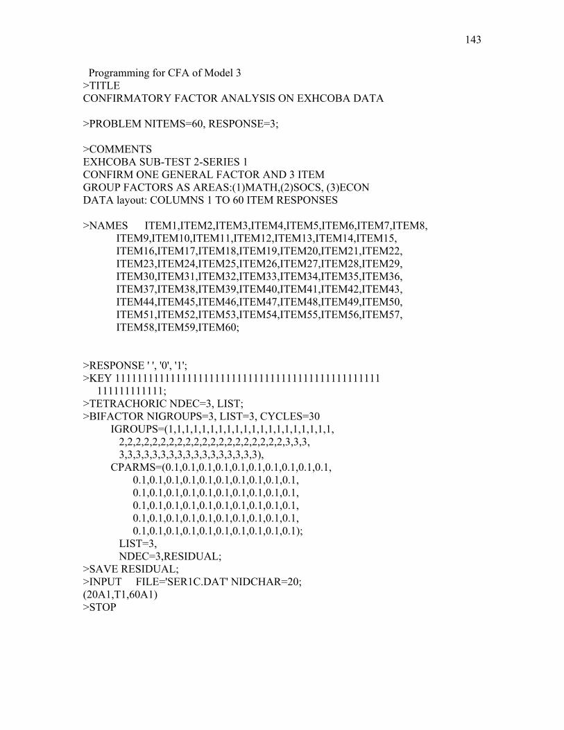
143

Programming for CFA of Model 3 >TITLE CONFIRMATORY FACTOR ANALYSIS ON EXHCOBA DATA >PROBLEM NITEMS=60, RESPONSE=3; >COMMENTS EXHCOBA SUB-TEST 2-SERIES 1 CONFIRM ONE GENERAL FACTOR AND 3 ITEM GROUP FACTORS AS AREAS:(1)MATH,(2)SOCS, (3)ECON DATA layout: COLUMNS 1 TO 60 ITEM RESPONSES >NAMES ITEM1,ITEM2,ITEM3,ITEM4,ITEM5,ITEM6,ITEM7,ITEM8, ITEM9,ITEM10,ITEM11,ITEM12,ITEM13,ITEM14,ITEM15, ITEM16,ITEM17,ITEM18,ITEM19,ITEM20,ITEM21,ITEM22, ITEM23,ITEM24,ITEM25,ITEM26,ITEM27,ITEM28,ITEM29, ITEM30,ITEM31,ITEM32,ITEM33,ITEM34,ITEM35,ITEM36, ITEM37,ITEM38,ITEM39,ITEM40,ITEM41,ITEM42,ITEM43, ITEM44,ITEM45,ITEM46,ITEM47,ITEM48,ITEM49,ITEM50, ITEM51,ITEM52,ITEM53,ITEM54,ITEM55,ITEM56,ITEM57, ITEM58,ITEM59,ITEM60; >RESPONSE ' ', '0', '1'; >KEY 111111111111111111111111111111111111111111111111 111111111111; >TETRACHORIC NDEC=3, LIST; >BIFACTOR NIGROUPS=3, LIST=3, CYCLES=30 IGROUPS=(1,1,1,1,1,1,1,1,1,1,1,1,1,1,1,1,1,1,1,1, 2,2,2,2,2,2,2,2,2,2,2,2,2,2,2,2,2,2,2,2,3,3,3, 3,3,3,3,3,3,3,3,3,3,3,3,3,3,3,3,3), CPARMS=(0.1,0.1,0.1,0.1,0.1,0.1,0.1,0.1,0.1,0.1, 0.1,0.1,0.1,0.1,0.1,0.1,0.1,0.1,0.1,0.1, 0.1,0.1,0.1,0.1,0.1,0.1,0.1,0.1,0.1,0.1, 0.1,0.1,0.1,0.1,0.1,0.1,0.1,0.1,0.1,0.1, 0.1,0.1,0.1,0.1,0.1,0.1,0.1,0.1,0.1,0.1, 0.1,0.1,0.1,0.1,0.1,0.1,0.1,0.1,0.1,0.1); LIST=3, NDEC=3,RESIDUAL; >SAVE RESIDUAL; >INPUT FILE='SER1C.DAT' NIDCHAR=20; (20A1,T1,60A1) >STOP

144

APPENDIX III

The Rasch modeling findings for the subscales in the career area knowledge are

presented in this subsection:

a) Science – Engineering Program:

Table 22

Item Calibrations for EXHCOBA Items 191-210 Math-Calculus


INFIT ZSTD

OUTFIT MSQ


1 0.09 0.1 1.28 6.51 1.42 6.07 0.26 0.3 2 -0.25 0.1 1 0.01 0.97 -0.52 0.47 1.02 3 -0.66 0.1 1.02 0.58 0.99 -0.14 0.44 0.96 4 0.19 0.1 1.06 1.53 1.04 0.58 0.43 0.88 5 -1.26 0.1 0.89 -2.49 0.8 -2.25 0.51 1.22 6 1.51 0.12 1.1 1.52 1.18 1.36 0.35 0.88 7 -0.03 0.1 0.95 -1.2 0.93 -1.22 0.5 1.12 8 -0.78 0.1 0.87 -3.55 0.82 -2.63 0.54 1.33 9 -0.95 0.1 0.91 -2.33 0.85 -1.96 0.51 1.22

10 -0.3 0.1 0.87 -3.56 0.81 -3.29 0.55 1.35 11 0.43 0.1 0.95 -1.27 0.95 -0.78 0.5 1.11 12 0.61 0.1 0.97 -0.67 1.02 0.21 0.48 1.04 13 -0.37 0.1 0.89 -3.17 0.82 -3.06 0.54 1.32 14 0.17 0.1 1.22 5.01 1.26 3.86 0.32 0.5 15 0.76 0.1 0.93 -1.42 0.9 -1.29 0.51 1.12 16 0.63 0.1 1.03 0.6 1.05 0.71 0.44 0.94 17 -1.37 0.1 0.97 -0.68 1.08 0.73 0.43 1.04 18 -0.18 0.1 1.04 0.98 1.13 2.13 0.43 0.87 19 1.52 0.12 1.16 2.24 1.35 2.58 0.3 0.8 20 0.23 0.1 0.89 -2.87 0.84 -2.69 0.55 1.27

Note: Tables in this appendix are interpreted as follows: for INFIT MSQ and OUTFIT MSQ model

expectation values are between 1 and 1.3. For INFIT ZSTD and OUTFIT ZSTD model expectation

values range between -2 to + 2. Values departing from these limits are highlighted in bold.

CORR indicates the biserial correlation between the each dichotomously scored item and the total score for

the item. Higher CORR values are an indication of scale unidimensionality. DISCR is an indication of the

item’s discrimination power.

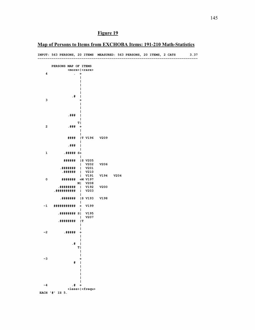
145

Figure 19

Map of Persons to Items from EXCHOBA Items: 191-210 Math-Statistics

INPUT: 563 PERSONS, 20 ITEMS MEASURED: 563 PERSONS, 20 ITEMS, 2 CATS 3.37 -------------------------------------------------------------------------------- PERSONS MAP OF ITEMS <more>|<rare> 4 . + | | | | | .# | 3 + | | | .### | | T| 2 .### + | | #### |T V196 V209 | .### | | 1 .##### S+ | ###### |S V205 | V202 V206 .####### | V201 .###### | V210 | V191 V194 V204 0 ####### +M V197 M| V208 .######## | V192 V200 .########## | V203 | .####### |S V193 V198 | -1 ########### + V199 | .######## S| V195 | V207 .######## |T | | -2 .##### + | | .# | T| | | -3 + # | | | | | | -4 .# + <less>|<frequ> EACH '#' IS 5.

146

Table 24

Item Calibrations for EXHCOBA Items 231-250 Chemistry


INFIT ZSTD

OUTFIT MSQ


1 1.02 0.12 1.04 0.57 1.15 1.36 0.19 0.94 2 0.93 0.12 0.95 -0.75 0.95 -0.55 0.3 1.06 3 0.07 0.1 1 -0.08 0.97 -0.57 0.32 1.03 4 -0.36 0.09 0.96 -1.26 0.95 -1.38 0.37 1.17 5 -0.45 0.09 0.93 -2.49 0.9 -2.7 0.41 1.33 6 -0.59 0.09 1.09 3.18 1.09 2.36 0.27 0.64 7 -0.77 0.09 1 -0.17 0.99 -0.37 0.36 1.06 8 0.76 0.11 1.02 0.34 1.17 1.82 0.23 0.96 9 -0.39 0.09 0.98 -0.76 0.96 -1.06 0.36 1.12

10 0.02 0.1 1.06 1.55 1.11 1.97 0.25 0.83 11 0.34 0.1 1.02 0.51 0.99 -0.12 0.28 0.97 12 0.75 0.11 0.97 -0.44 1.01 0.13 0.28 1.03 13 -0.8 0.09 0.96 -1.48 0.96 -1.21 0.4 1.2 14 -0.28 0.09 1.03 1.05 1.03 0.76 0.3 0.9 15 -0.57 0.09 1 -0.14 1.02 0.55 0.35 1.02 16 1.14 0.12 0.99 -0.07 0.98 -0.17 0.24 1.01 17 0.08 0.1 1.03 0.81 1 0.07 0.29 0.95 18 -0.45 0.09 0.97 -1.07 0.96 -0.98 0.37 1.15 19 0.17 0.1 0.99 -0.37 1 -0.02 0.32 1.04 20 -0.62 0.09 1 -0.08 1.01 0.23 0.35 1.03







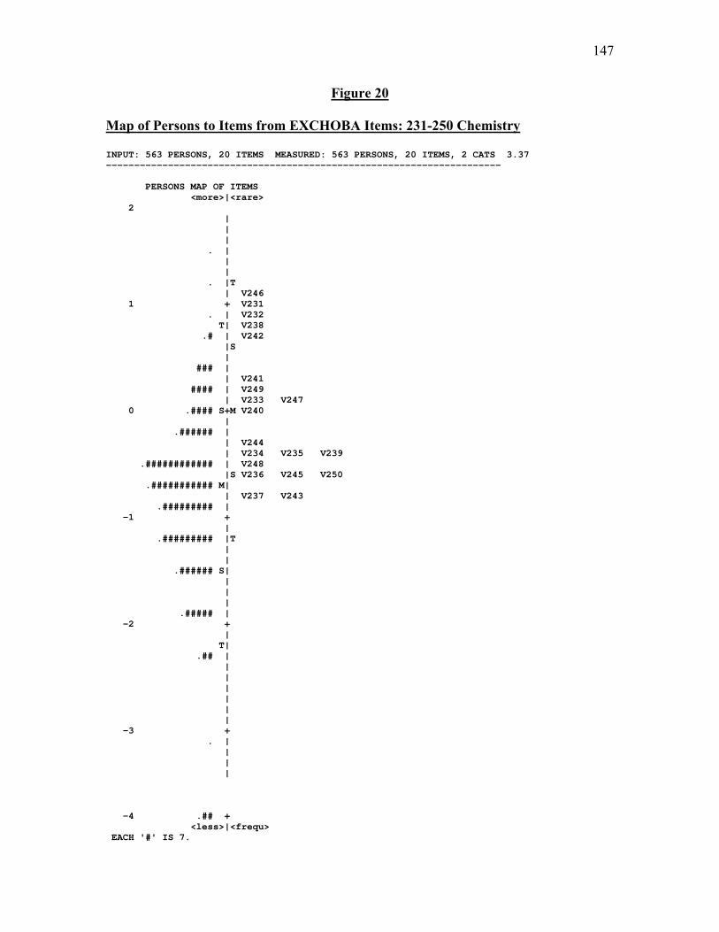
147

Figure 20

Map of Persons to Items from EXCHOBA Items: 231-250 Chemistry

INPUT: 563 PERSONS, 20 ITEMS MEASURED: 563 PERSONS, 20 ITEMS, 2 CATS 3.37 ---------------------------------------------------------------------- PERSONS MAP OF ITEMS <more>|<rare> 2 | | | . | | | . |T | V246 1 + V231 . | V232 T| V238 .# | V242 |S | ### | | V241 #### | V249 | V233 V247 0 .#### S+M V240 | .###### | | V244 | V234 V235 V239 .############ | V248 |S V236 V245 V250 .########### M| | V237 V243 .######### | -1 + | .######### |T | | .###### S| | | | .##### | -2 + | T| .## | | | | | | | -3 + . | | | | -4 .## + <less>|<frequ> EACH '#' IS 7.

148

Table 25

Item Calibrations for EXHCOBA Items 251-270 Physics


INFIT ZSTD

OUTFIT MSQ


1 -0.73 0.09 1.01 0.27 0.99 -0.18 0.37 1 2 0.27 0.09 0.97 -0.89 0.96 -0.87 0.36 1.11 3 0.8 0.1 1.02 0.35 1.01 0.11 0.28 0.97 4 -0.68 0.09 1.02 0.52 1 0.04 0.36 0.97 5 0.63 0.1 1.06 1.38 1.08 1.2 0.25 0.87 6 0.62 0.1 1.02 0.53 0.98 -0.37 0.3 0.97 7 -0.04 0.09 1.11 3.83 1.13 3.03 0.24 0.53 8 0.02 0.09 1.1 3.47 1.19 4.16 0.23 0.54 9 0.25 0.09 0.9 -3.08 0.87 -2.89 0.43 1.35

10 -0.22 0.09 0.96 -1.59 0.97 -0.7 0.39 1.19 11 0.33 0.09 0.98 -0.45 0.97 -0.57 0.34 1.05 12 0.35 0.09 0.98 -0.71 0.94 -1.17 0.35 1.1 13 -0.31 0.09 0.98 -0.68 0.97 -0.65 0.38 1.11 14 0.85 0.1 0.98 -0.43 1.01 0.09 0.31 1.04 15 -0.69 0.09 0.91 -3.15 0.88 -2.98 0.46 1.36 16 -0.52 0.09 1 0.14 1.01 0.13 0.36 0.99 17 -0.75 0.09 1.07 2.13 1.16 3.4 0.3 0.75 18 -0.32 0.09 0.98 -0.73 1 -0.06 0.37 1.08 19 -0.34 0.09 0.86 -5.19 0.83 -4.71 0.49 1.63 20 0.47 0.1 1.09 2.33 1.13 2.21 0.23 0.75







149

Figure 21

Map of Persons to Items from EXCHOBA Items: 251-270 Physics

INPUT: 563 PERSONS, 20 ITEMS MEASURED: 563 PERSONS, 20 ITEMS, 2 CATS PERSONS MAP OF ITEMS <more>|<rare> 3 . + | | | | | | 2 + | | | .# | T| .# | 1 +T .# | V253 V264 .#### | S|S V255 V256 .####### | V270 | V252 V259 V261 V262 .##### | 0 ######## +M V257 V258 | .########### M| V260 V263 V268 V269 .########### | |S V266 .####### | V251 V254 V265 V267 ###### | -1 +T .#### S| | .### | | | ### T| -2 + | . | | | | | -3 . + | | | | | | -4 .# + <less>|<frequ> EACH '#' IS 7.

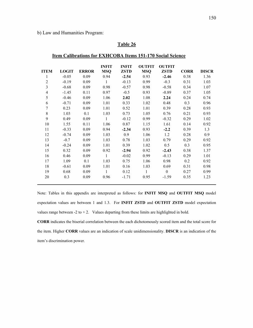
150

b) Law and Humanities Program:

Table 26

Item Calibrations for EXHCOBA Items 151-170 Social Science


INFIT ZSTD

OUTFIT MSQ


1 -0.05 0.09 0.94 -2.54 0.93 -2.46 0.38 1.36 2 -0.19 0.09 1 -0.13 0.99 -0.3 0.31 1.03 3 -0.68 0.09 0.98 -0.57 0.98 -0.58 0.34 1.07 4 -1.45 0.11 0.97 -0.5 0.93 -0.89 0.37 1.05 5 -0.46 0.09 1.06 2.02 1.08 2.24 0.24 0.74 6 -0.71 0.09 1.01 0.33 1.02 0.48 0.3 0.96 7 0.23 0.09 1.01 0.52 1.01 0.39 0.28 0.93 8 1.03 0.1 1.03 0.73 1.05 0.76 0.21 0.93 9 0.49 0.09 1 -0.12 0.99 -0.32 0.29 1.02

10 1.55 0.11 1.06 0.87 1.15 1.61 0.14 0.92 11 -0.33 0.09 0.94 -2.34 0.93 -2.2 0.39 1.3 12 -0.74 0.09 1.03 0.9 1.06 1.2 0.28 0.9 13 -0.7 0.09 1.03 0.78 1.03 0.79 0.29 0.92 14 -0.24 0.09 1.01 0.39 1.02 0.5 0.3 0.95 15 0.32 0.09 0.92 -2.94 0.92 -2.43 0.38 1.37 16 0.46 0.09 1 -0.02 0.99 -0.13 0.29 1.01 17 1.09 0.1 1.03 0.75 1.06 0.98 0.2 0.92 18 -0.61 0.09 1.01 0.16 1.03 0.69 0.31 0.98 19 0.68 0.09 1 0.12 1 0 0.27 0.99 20 0.3 0.09 0.96 -1.71 0.95 -1.59 0.35 1.23







151

Figure 22


INPUT: 582 PERSONS, 20 ITEMS MEASURED: 582 PERSONS, 20 ITEMS, 2 CATS ----------------------------------------------------------------------- PERSONS MAP OF ITEMS <more>|<rare> 3 + | | | | . | | | 2 + | | | . |T V160 T| .## | | V167 1 .#### + V158 | .##### |S S| V169 .###### | V159 V166 | V165 .########## | V157 V170 | 0 .######## M+M V151 | V152 .############ | V164 | V161 ######## | V155 | V153 V168 ##### S|S V156 V162 V163 | -1 #### + | .# | T| .# |T V154 | | . | -2 + | | . | | | | | -3 + . | | | | | | | -4 . + <less>|<frequ> EACH '#' IS 8.

152

Table 27

Item Calibrations for EXHCOBA Items 271-290 Language


INFIT ZSTD

OUTFIT MSQ


1 -0.83 0.1 0.96 -0.75 0.96 -0.54 0.42 1.07 2 -0.1 0.09 0.99 -0.27 0.96 -0.83 0.39 1.05 3 -0.67 0.1 0.89 -2.71 0.82 -2.86 0.49 1.25 4 -0.03 0.09 0.97 -1.05 0.96 -0.84 0.4 1.12 5 0.92 0.09 0.95 -1.55 0.92 -1.4 0.39 1.16 6 0.05 0.09 1.01 0.29 1 -0.07 0.37 0.98 7 -0.47 0.09 0.94 -1.54 0.96 -0.69 0.43 1.14 8 -1.18 0.11 0.95 -0.93 0.92 -0.92 0.44 1.08 9 -0.07 0.09 1.07 2.35 1.07 1.4 0.32 0.76

10 -1.86 0.13 0.97 -0.33 0.91 -0.65 0.43 1.03 11 -0.1 0.09 1.08 2.5 1.14 2.85 0.3 0.7 12 -0.39 0.09 1.02 0.56 1.09 1.53 0.36 0.92 13 1.06 0.09 1 0.02 1.01 0.21 0.33 0.99 14 -0.17 0.09 0.98 -0.63 1.01 0.16 0.39 1.06 15 0.12 0.09 1.07 2.47 1.08 1.76 0.31 0.72 16 -0.04 0.09 0.96 -1.3 0.96 -0.88 0.41 1.14 17 1.6 0.1 1.07 1.35 1.18 2.03 0.22 0.86 18 -0.02 0.09 0.92 -2.71 0.98 -0.35 0.44 1.26 19 0.72 0.09 1.04 1.39 1.1 2.01 0.3 0.82 20 1.46 0.1 1.07 1.48 1.11 1.31 0.24 0.87







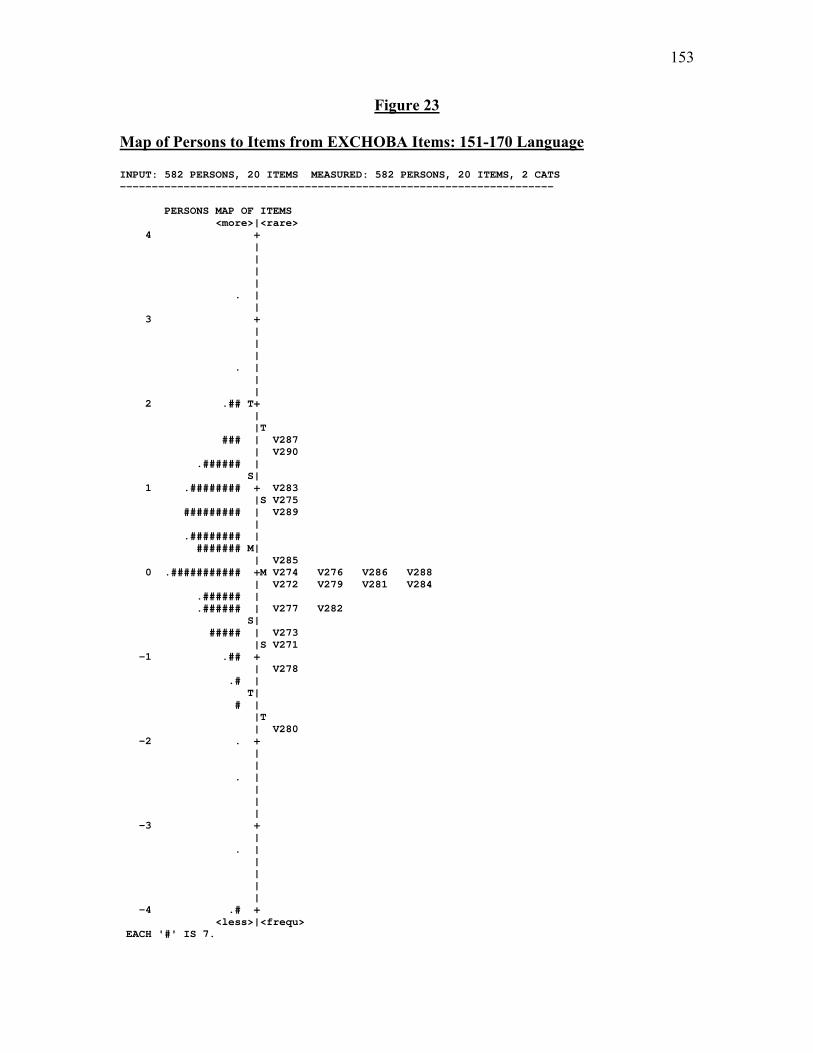
153

Figure 23


INPUT: 582 PERSONS, 20 ITEMS MEASURED: 582 PERSONS, 20 ITEMS, 2 CATS -------------------------------------------------------------------- PERSONS MAP OF ITEMS <more>|<rare> 4 + | | | | . | | 3 + | | | . | | | 2 .## T+ | |T ### | V287 | V290 .###### | S| 1 .######## + V283 |S V275 ######### | V289 | .######## | ####### M| | V285 0 .########### +M V274 V276 V286 V288 | V272 V279 V281 V284 .###### | .###### | V277 V282 S| ##### | V273 |S V271 -1 .## + | V278 .# | T| # | |T | V280 -2 . + | | . | | | | -3 + | . | | | | | -4 .# + <less>|<frequ> EACH '#' IS 7.

154

Table 28

Item Calibrations for EXHCOBA Items 291-310 Humanities

ITEM LOGIT ERROR IN.MSQ INFIT ZSTD

OUTFIT MSQ


1 -0.92 0.1 0.96 -0.84 0.95 -0.75 0.38 1.08 2 0.78 0.09 1.06 1.72 1.06 1.05 0.27 0.83 3 -0.67 0.09 0.96 -0.97 0.96 -0.77 0.38 1.09 4 0.3 0.09 1.09 3.12 1.11 2.75 0.25 0.61 5 0.3 0.09 1.01 0.49 1.01 0.36 0.33 0.94 6 -0.37 0.09 0.98 -0.7 0.97 -0.58 0.37 1.08 7 0.35 0.09 1.09 3.11 1.11 2.6 0.24 0.61 8 -1.37 0.11 1.02 0.26 0.98 -0.27 0.32 0.99 9 -0.01 0.09 1.01 0.39 1 0.04 0.34 0.97

10 0.65 0.09 0.91 -2.96 0.88 -2.73 0.44 1.32 11 0.69 0.09 1.02 0.54 1 0 0.32 0.96 12 0.49 0.09 1 -0.12 0.98 -0.48 0.35 1.03 13 -0.03 0.09 0.98 -0.55 1.01 0.22 0.36 1.06 14 0.6 0.09 0.98 -0.58 0.96 -0.78 0.36 1.07 15 -0.67 0.09 0.95 -1.38 0.93 -1.22 0.4 1.14 16 0.08 0.09 1.03 1.11 1.07 1.75 0.31 0.85 17 -1.27 0.1 0.97 -0.51 0.93 -0.91 0.36 1.05 18 -0.28 0.09 0.99 -0.33 0.98 -0.52 0.36 1.05 19 1.26 0.1 1.06 1.3 1.1 1.32 0.24 0.88 20 0.11 0.09 0.93 -2.74 0.93 -1.93 0.42 1.33







155

Figure 24

Map of Persons to Items from EXCHOBA Items: 291-310 Humanities

INPUT: 582 PERSONS, 20 ITEMS MEASURED: 582 PERSONS, 20 ITEMS, 2 CATS ----------------------------------------------------------------------- PERSONS MAP OF ITEMS <more>|<rare> 4 . + | | | | | . | 3 + | | | . | | | 2 + # | T| .### | |T | V309 ##### | 1 .###### + S| ########### |S V292 V300 V301 | V304 .######### | V302 .########## | V294 V295 V297 M| V306 V310 0 .########### +M V299 V303 .########## | | V308 .######## | V296 | .####### S|S V293 V305 | V291 -1 .#### + .### | | V307 |T V298 .## T| | . | -2 + | | . | | | | -3 + . | | | | | | -4 . + <less>|<frequ> EACH '#' IS 6.

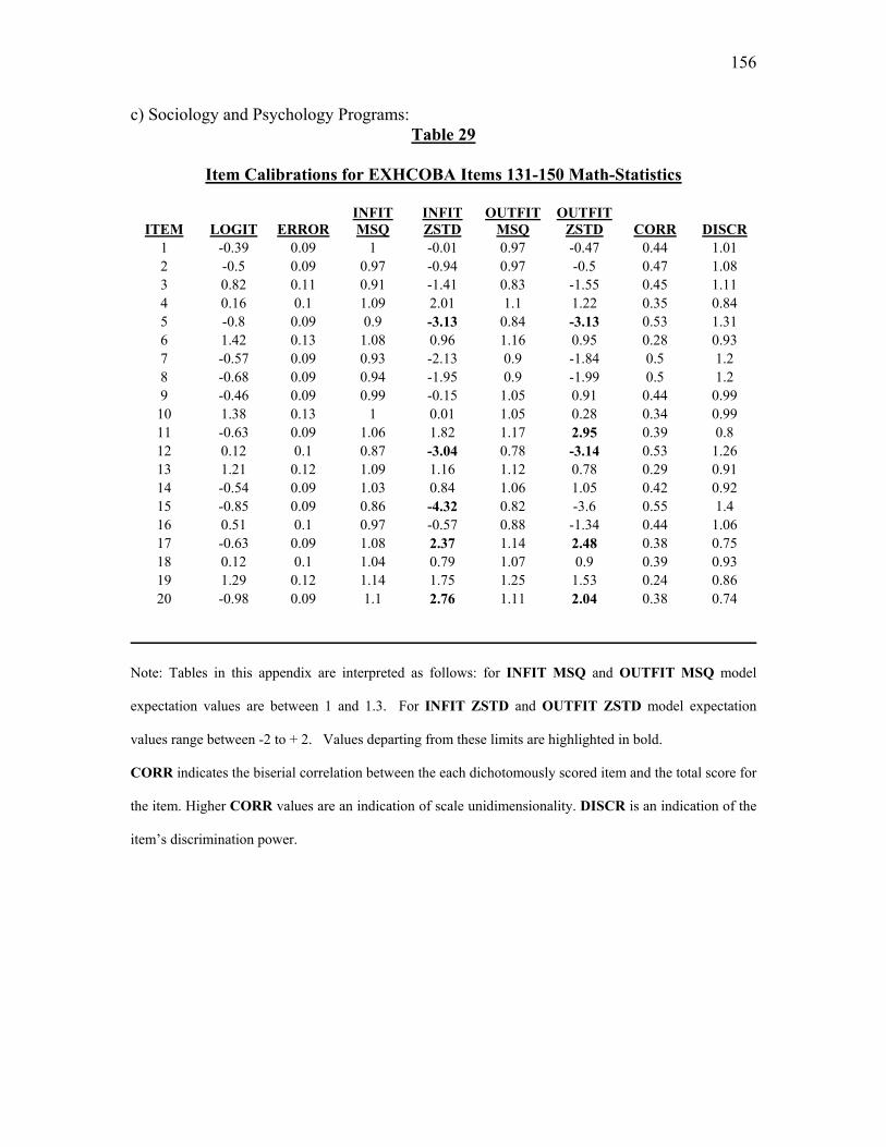
156

c) Sociology and Psychology Programs: Table 29

Item Calibrations for EXHCOBA Items 131-150 Math-Statistics


INFIT ZSTD

OUTFIT MSQ


1 -0.39 0.09 1 -0.01 0.97 -0.47 0.44 1.01 2 -0.5 0.09 0.97 -0.94 0.97 -0.5 0.47 1.08 3 0.82 0.11 0.91 -1.41 0.83 -1.55 0.45 1.11 4 0.16 0.1 1.09 2.01 1.1 1.22 0.35 0.84 5 -0.8 0.09 0.9 -3.13 0.84 -3.13 0.53 1.31 6 1.42 0.13 1.08 0.96 1.16 0.95 0.28 0.93 7 -0.57 0.09 0.93 -2.13 0.9 -1.84 0.5 1.2 8 -0.68 0.09 0.94 -1.95 0.9 -1.99 0.5 1.2 9 -0.46 0.09 0.99 -0.15 1.05 0.91 0.44 0.99

10 1.38 0.13 1 0.01 1.05 0.28 0.34 0.99 11 -0.63 0.09 1.06 1.82 1.17 2.95 0.39 0.8 12 0.12 0.1 0.87 -3.04 0.78 -3.14 0.53 1.26 13 1.21 0.12 1.09 1.16 1.12 0.78 0.29 0.91 14 -0.54 0.09 1.03 0.84 1.06 1.05 0.42 0.92 15 -0.85 0.09 0.86 -4.32 0.82 -3.6 0.55 1.4 16 0.51 0.1 0.97 -0.57 0.88 -1.34 0.44 1.06 17 -0.63 0.09 1.08 2.37 1.14 2.48 0.38 0.75 18 0.12 0.1 1.04 0.79 1.07 0.9 0.39 0.93 19 1.29 0.12 1.14 1.75 1.25 1.53 0.24 0.86 20 -0.98 0.09 1.1 2.76 1.11 2.04 0.38 0.74







157

Figure 25

Map of Persons to Items from EXCHOBA Items: 131-150 Math-Statistics

INPUT: 626 PERSONS, 20 ITEMS MEASURED: 626 PERSONS, 20 ITEMS, 2 CATS ---------------------------------------------------------------------- PERSONS MAP OF ITEMS <more>|<rare> 4 . + | | | | . | | 3 + | | | . | | | 2 . + | | . |T T| V136 V140 .# | V143 V149 | 1 .### + |S V133 .### | | V146 .## | S| .##### | V134 V142 V148 0 ##### +M | .####### | .######## | V131 V132 V139 | V137 V141 V144 V147 .######## | V138 M|S V135 V145 -1 .############ + V150 | ########### | | .########## |T | | -2 .####### S+ | | .###### | | | | -3 + ###### T| | | | | | -4 .# + <less>|<frequ> EACH '#' IS 6.

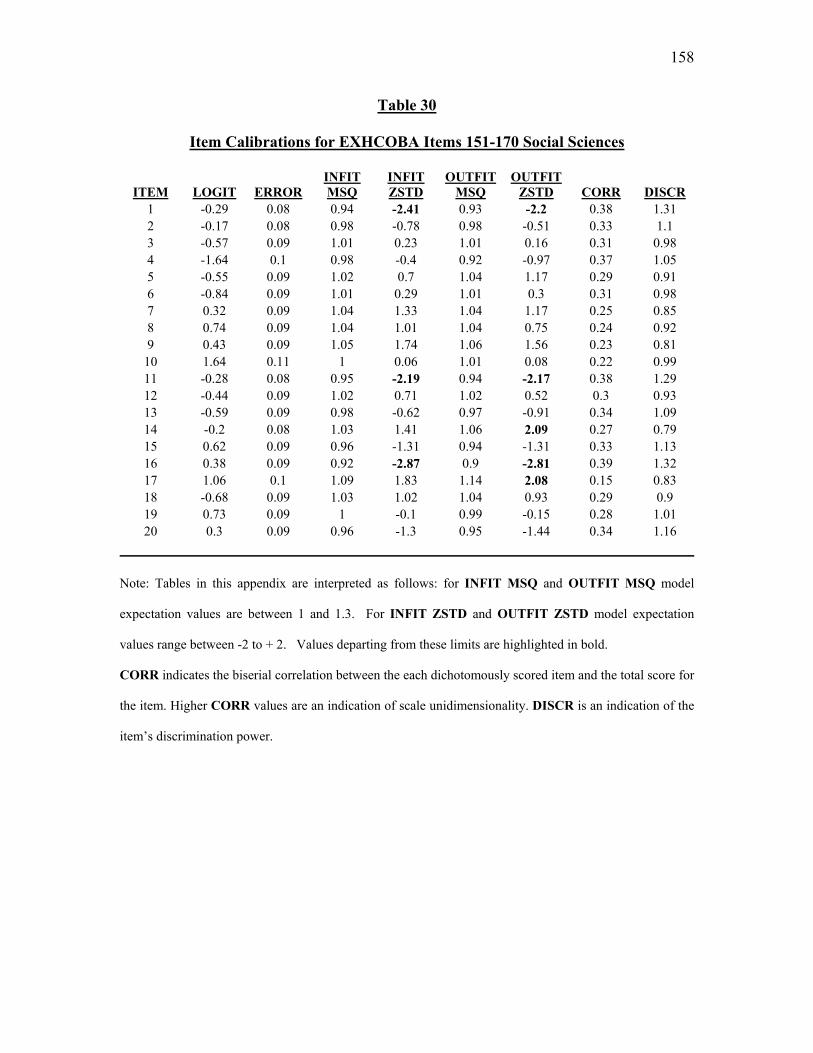
158

Table 30

Item Calibrations for EXHCOBA Items 151-170 Social Sciences


INFIT ZSTD

OUTFIT MSQ


1 -0.29 0.08 0.94 -2.41 0.93 -2.2 0.38 1.31 2 -0.17 0.08 0.98 -0.78 0.98 -0.51 0.33 1.1 3 -0.57 0.09 1.01 0.23 1.01 0.16 0.31 0.98 4 -1.64 0.1 0.98 -0.4 0.92 -0.97 0.37 1.05 5 -0.55 0.09 1.02 0.7 1.04 1.17 0.29 0.91 6 -0.84 0.09 1.01 0.29 1.01 0.3 0.31 0.98 7 0.32 0.09 1.04 1.33 1.04 1.17 0.25 0.85 8 0.74 0.09 1.04 1.01 1.04 0.75 0.24 0.92 9 0.43 0.09 1.05 1.74 1.06 1.56 0.23 0.81

10 1.64 0.11 1 0.06 1.01 0.08 0.22 0.99 11 -0.28 0.08 0.95 -2.19 0.94 -2.17 0.38 1.29 12 -0.44 0.09 1.02 0.71 1.02 0.52 0.3 0.93 13 -0.59 0.09 0.98 -0.62 0.97 -0.91 0.34 1.09 14 -0.2 0.08 1.03 1.41 1.06 2.09 0.27 0.79 15 0.62 0.09 0.96 -1.31 0.94 -1.31 0.33 1.13 16 0.38 0.09 0.92 -2.87 0.9 -2.81 0.39 1.32 17 1.06 0.1 1.09 1.83 1.14 2.08 0.15 0.83 18 -0.68 0.09 1.03 1.02 1.04 0.93 0.29 0.9 19 0.73 0.09 1 -0.1 0.99 -0.15 0.28 1.01 20 0.3 0.09 0.96 -1.3 0.95 -1.44 0.34 1.16







159

Figure 26


INPUT: 626 PERSONS, 20 ITEMS MEASURED: 626 PERSONS, 20 ITEMS, 2 CATS ----------------------------------------------------------------------- PERSONS MAP OF ITEMS <more>|<rare> 2 + . | | | | V160 | . |T | | .## T| | | V167 1 + .### | | |S V158 V169 .##### | S| V165 | .######## | V159 V166 | V157 V170 .########## | | | 0 .############ +M | M| V152 V164 ############# | V151 V161 | .########## | V162 | | V153 V155 V163 ######## | V168 |S S| V156 .###### | -1 + | | .#### | | | .# T|T | | V154 | | . | -2 + | | | | . | | | -3 .# + <less>|<frequ> EACH '#' IS 7.

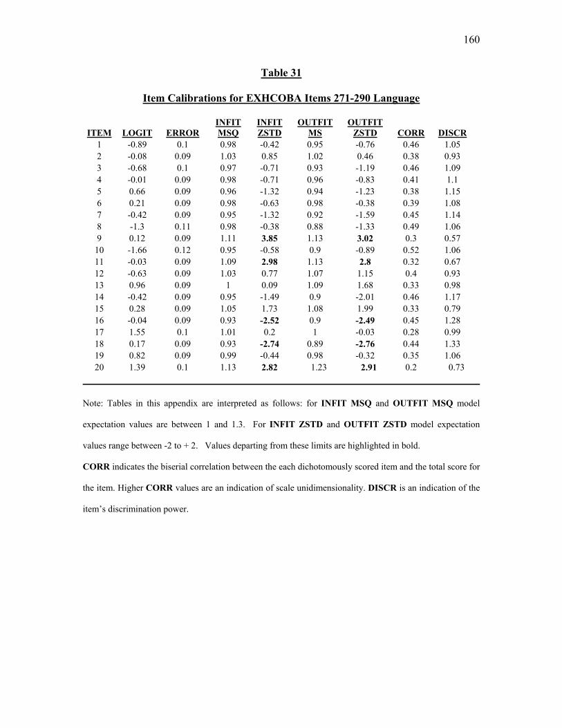
160

Table 31

Item Calibrations for EXHCOBA Items 271-290 Language


INFIT ZSTD

OUTFIT MS


1 -0.89 0.1 0.98 -0.42 0.95 -0.76 0.46 1.05 2 -0.08 0.09 1.03 0.85 1.02 0.46 0.38 0.93 3 -0.68 0.1 0.97 -0.71 0.93 -1.19 0.46 1.09 4 -0.01 0.09 0.98 -0.71 0.96 -0.83 0.41 1.1 5 0.66 0.09 0.96 -1.32 0.94 -1.23 0.38 1.15 6 0.21 0.09 0.98 -0.63 0.98 -0.38 0.39 1.08 7 -0.42 0.09 0.95 -1.32 0.92 -1.59 0.45 1.14 8 -1.3 0.11 0.98 -0.38 0.88 -1.33 0.49 1.06 9 0.12 0.09 1.11 3.85 1.13 3.02 0.3 0.57

10 -1.66 0.12 0.95 -0.58 0.9 -0.89 0.52 1.06 11 -0.03 0.09 1.09 2.98 1.13 2.8 0.32 0.67 12 -0.63 0.09 1.03 0.77 1.07 1.15 0.4 0.93 13 0.96 0.09 1 0.09 1.09 1.68 0.33 0.98 14 -0.42 0.09 0.95 -1.49 0.9 -2.01 0.46 1.17 15 0.28 0.09 1.05 1.73 1.08 1.99 0.33 0.79 16 -0.04 0.09 0.93 -2.52 0.9 -2.49 0.45 1.28 17 1.55 0.1 1.01 0.2 1 -0.03 0.28 0.99 18 0.17 0.09 0.93 -2.74 0.89 -2.76 0.44 1.33 19 0.82 0.09 0.99 -0.44 0.98 -0.32 0.35 1.06 20 1.39 0.1 1.13 2.82 1.23 2.91 0.2 0.73







161

Figure 27


INPUT: 626 PERSONS, 20 ITEMS MEASURED: 626 PERSONS, 20 ITEMS, 2 CATS ---------------------------------------------------------------------- PERSONS MAP OF ITEMS <more>|<rare> 4 + | | | | . | | 3 + | | | .# | | | 2 .## T+ | | .#### |T V287 | V290 .####### | S| 1 .########## + V283 |S V289 .########### | V275 | .############ | .########## M| V276 V285 | V279 V288 0 .########## +M V274 V281 V286 | V272 .######### | .######## | V277 V284 S| V282 .### | V273 |S V271 -1 ### + | .## | V278 T| . |T | V280 | -2 . + | | . | | | | -3 + | . | | | | | -4 .### + <less>|<frequ> EACH '#' IS 6

162

REFERENCES

Antillón Macías L.E. (2003) . La Equiparación de las Tres Versiones del EXHCOBA.

[Equating the Three Versions of EXHCOBA] Tesis de Maestría, Instituto de

Investigación y Desarrollo Educativo. Unidad Ensenada: Universidad

Autónoma de Baja California.

Backhoff, E., & Tirado, F. (1992) . Desarrollo del Examen de Habilidades y

Conocimientos Básicos [Development of the EXCHOBA]. Revista de la

Educación Superior, XXi(83), 95-118. (Available from Asociación Nacional de

Universidades e Instituciones de Educación Superior (ANUIES), México, D.F.)

Backhoff, E., & Tirado, F. (1993) . Habilidades y Conocimientos Básicos del Estudiante

Universitario: Hacia Estándares Nacionales [Basic Abilities and Knowledge in the

University Student: Towards National Standards]. Revista de la Educación

Superior, XXII(88), 45-65. (Available from Asociación Nacional de

Universidades e Instituciones de Educación Superior (ANUIES), México, D.F.)

Backhoff, E. E. (2001) . Desarrollo, Validacion e Implementacion de un Sistema de

Selección de Estudiantes en la Universidad Autonoma de Baja California. Tesis

Doctoral, Universidad Autónoma de Aguascalientes, Centro de Ciencias y

Humanidades, Doctorado Interinstitucional en Educación.

Bock, D., Gibbons, R., & Muraki, E. (1988) . Full Information Item Factor Analysis.

Applied Psychological Measurement. vol.13, no.3. pp. 261-280.

Bond, T.G., Fox, Ch. M. (2001) . Applying The Rasch Model: Fundamental Measurement

in the Human Sciences. New Jersey: Erlbaum.

163

Burgos, B. (2003) . Indicadores de los Procesos Educativos [Indicators of Eucational

Processes, Working document, ANUIES Noroeste, UNISON Dirección de

Planeación].

Cizek, G. J. (2001) . Setting Performance Standards: Concepts, Methods and

Perspectives. New Jersey: Erlbaum.

du Toit, M. Ed. (2003) . IRT from SSI BILOG-MG MULTILOG PARSCALE TESTFACT

Lincolnwood, IL: Scientific Software International.

Embretson, S.E., Reise, S,P. (2000) . Item Response Theory for Psychologists. New

Jersey: Erlbaum.

Gonzalez, L. , Lopez, L. (2004) . Perfil de Ingreso de los Estudiantes de la Universidad

de Sonora Ciclo 2003. Documentos de Investigación Educativa. Hermosillo, Son:

Universidad de Sonora.

Hambleton, R.K., Swaminathan, H., Rogers,J. H (1991) . Fundamentals of Item Response

Theory. Quantitative Methods for the Social Sciences. Newbury Park, CA: Sage

Publications.

Hill, H.C., Schilling, S.G., Loewenberg, D. (2004) . Developing Measures of Teachers’

Mathematics Knowledge for Teaching. The Elementary School Journal. vol. 105,

no. 1. pp.11-30.

Knol, D.K., Berger, M. (1991) . Empirical Comparisons Between Factor Analysis and

Multidimensional Item Response Models. Multivariate Behavioral Research, 26

(3) pp. 457-477.

164

Larrazolo R. N. (2004) . Resulatdos EXHCOBA 2004 en la Universidad de Sonora.

Reporte Técnico. Instituto de Investigación y Desarrollo Educativo. Campus

Ensenada: Universidad Autonoma de Baja California,.

Linacre, J. M. (2003) . A User's Guide to Winsteps Ministeps: Rasch-Model Computer

Programs. Chicago, IL: Electronic Publication.

Martinez R. F. (2001) . Evaluación Educativa y Pruebas Estandarizadas: Elementos para

Enriquecer el Debate. Revista de la Educación Superior, XXX (4) Octubre-

Diciembre.

Tirado, F., Backhoff, E., Larrazolo, N., & Rosas, M. (1997) . Validez Predictiva del

Examen de Habilidades y Conocimientos Basicos [Predictive Validity of

EXHCOBA]. Revista Mexicana de Investigación Educativa, II(3), Enero - Junio.

Universidad de Sonora. (2001) . Plan de Desarrollo Institucional 2001-2005 [Plan for

Institutional Development 2001-2005]. (Available from Dirección de Planeación,

Blvd. Rosales y Transversal, Hermosillo, Sonora, Mexico).

Webb, N. L. (1999) . Alignment of Science and Mathematics Standards and Assessments

in Four States. National Institute for Science Education, University of

Winsconsin-Madison, Washington, D.C: Council of Chief State School Offices,

Wright, B. D., & Stone, M. H. (1979) . Best Test Design. Chicago, IL: MESA Press.

DEFINING AND MEASURING ACADEMIC STANDARDS · PDF fileentitled Defining and Measuring Academic...

Documents

Transcript of DEFINING AND MEASURING ACADEMIC STANDARDS · PDF fileentitled Defining and Measuring Academic...