Deep Sleep: Convolutional Neural Networks for PredictiveModeling of Human Sleep Time-Signals

Sarun PaisarnsrisomsukWorcester Polytechnic InstituteWorcester, Massachusetts, USAspaisarnsrisomsu@wpi.edu

Michael SokolovskyWorcester Polytechnic InstituteWorcester, Massachusetts, USA

sokolovsky@wpi.edu

Francisco GuerreroWorcester Polytechnic InstituteWorcester, Massachusetts, USAafguerrerohernan@wpi.edu

Carolina Ruiz∗Worcester Polytechnic InstituteWorcester, Massachusetts, USA

ruiz@wpi.edu

Sergio A. Alvarez∗†Boston College

Chestnut Hill, Massachusetts, USAalvarez@bc.edu

ABSTRACTWe discuss our work on predictive modeling in sleep medicineusing deep learning, with attention to domain interpretation of theemergent internal features. More specifically, we describe a high-performing deep convolutional neural network (CNN) architecturefor classification of human sleep EEG and EOG signals into sleepstages, the classification performance of which amply exceeds thatof recently published CNN work that uses a single EEG channel.We show that the use of multiple signal channels accounts for onlya minor fraction of our network’s performance, and that the bulk ofits performance superiority relies on its greater depth as comparedwith alternate architectures. By visualizing the response profiles ofinternal layers of our network to carefully selected input signalsafter supervised learning, we show that the convolutional filtersin these layers extract signal features that closely resemble thoseused by human sleep experts in manually classifying sleep intostages, and that combine both time-domain and frequency-domainelements. We go on to describe the development of these featureswith layer depth, showing that the network assembles them instages, by extracting simple building blocks in shallow layers andcombining them in deeper layers to form more complex features.This phenomenon of hierarchical feature formation is well-knownin two-dimensional image classification using deep networks, buthas not previously been reported in sleep stage classification basedon time-varying one-dimensional signals.

CCS CONCEPTS• Computing methodologies → Neural networks; Supervisedlearning by classification; •Applied computing→Health infor-matics;

∗Senior authors.†Corresponding author.

Permission to make digital or hard copies of part or all of this work for personal orclassroom use is granted without fee provided that copies are not made or distributedfor profit or commercial advantage and that copies bear this notice and the full citationon the first page. Copyrights for third-party components of this work must be honored.For all other uses, contact the owner/author(s).KDD’18 Deep Learning Day, August 2018, London, UK© 2018 Copyright held by the owner/author(s).ACM ISBN 978-x-xxxx-xxxx-x/YY/MM.https://doi.org/10.1145/nnnnnnn.nnnnnnn

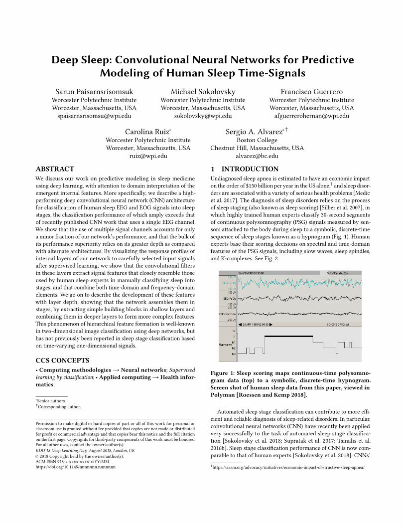
1 INTRODUCTIONUndiagnosed sleep apnea is estimated to have an economic impacton the order of $150 billion per year in the US alone,1 and sleep disor-ders are associated with a variety of serious health problems [Medicet al. 2017]. The diagnosis of sleep disorders relies on the processof sleep staging (also known as sleep scoring) [Silber et al. 2007], inwhich highly trained human experts classify 30-second segmentsof continuous polysomnography (PSG) signals measured by sen-sors attached to the body during sleep to a symbolic, discrete-timesequence of sleep stages known as a hypnogram (Fig. 1). Humanexperts base their scoring decisions on spectral and time-domainfeatures of the PSG signals, including slow waves, sleep spindles,and K-complexes. See Fig. 2.

Figure 1: Sleep scoring maps continuous-time polysomno-gram data (top) to a symbolic, discrete-time hypnogram.Screen shot of human sleep data from this paper, viewed inPolyman [Roessen and Kemp 2018].

Automated sleep stage classification can contribute to more effi-cient and reliable diagnosis of sleep-related disorders. In particular,convolutional neural networks (CNN) have recently been appliedvery successfully to the task of automated sleep stage classifica-tion [Sokolovsky et al. 2018; Supratak et al. 2017; Tsinalis et al.2016b]. Sleep stage classification performance of CNN is now com-parable to that of human experts [Sokolovsky et al. 2018]. CNNs’

1https://aasm.org/advocacy/initiatives/economic-impact-obstructive-sleep-apnea/

KDD’18 Deep Learning Day, August 2018, London, UK S. Paisarnsrisomsuk et al.

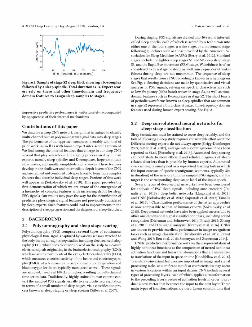
Figure 2: Sample of stage S2 sleep EEG, showing aK-complexfollowed by a sleep spindle. Total duration is 3s. Expert scor-ers rely on these and other time-domain and frequency-domain features to assign sleep samples to stages.

impressive predictive performance is, unfortunately, accompaniedby opaqueness of their internal mechanisms.

Contributions of this paperWe describe a deep CNN network design that is trained to classifymulti-channel human polysomnogram signal data into sleep stages.The performance of our approach compares favorably with that ofprior work, as well as with human expert inter-scorer agreement.We find among the internal features that emerge in our deep CNNseveral that play key roles in the staging process used by humanexperts, namely sleep spindles and K-complexes, large-amplitudeslow waves, and smaller-amplitude alpha waves. These featuresdevelop in the shallower and intermediate-depth layers of the CNNand are refined and combined in deeper layers to formmore complexfeatures that describe individual sleep stages. Portions of this workwill appear in [Sokolovsky et al. 2018]. This paper provides thefirst demonstration of which we are aware of the emergence ofa hierarchy of complex features with increasing depth for sleepEEG signals. Our results may pave the way for the identification ofpredictive physiological signal features not previously consideredby sleep experts. Such features could lead to improvements in thedescription of sleep progression and the diagnosis of sleep disorders.

2 BACKGROUND2.1 Polysomnography and sleep stage scoringPolysomnography (PSG) comprises several types of continuousphysiological time signals captured by various sensors attached tothe body during all-night sleep studies, including electroencephalog-raphy (EEG), which uses electrodes placed on the scalp to measureelectrical signals originating in the brain; electrooculography (EOG),which measures movements of the eyes; electrocardiography (ECG),which measures electrical activity of the heart; and electromyogra-phy (EMG), which measures muscle contractions. Respiration andblood oxygen levels are typically monitored, as well. These signalsare sampled, usually at 100 Hz or higher, resulting in multi-channeltime series data. Traditionally, highly trained human experts con-vert the sampled PSG signals visually to a symbolic representationin terms of a small number of sleep stages, via a classification pro-cess known as sleep staging or sleep scoring [Silber et al. 2007].

During staging, PSG signals are divided into 30-second intervalscalled sleep epochs, each of which is scored by a technician intoeither one of the four stages, a wake stage, or a movement stage,following guidelines such as those provided by the American As-sociation for Sleep Medicine (AASM) [Berry et al. 2012]. Standardstages include the lighter sleep stages S1 and S2, deep sleep stageS3, and the Rapid Eye movement (REM) stage. Wakefulness is oftenconsidered to be a stage of sleep, as well, since episodes of wake-fulness during sleep are not uncommon. The sequence of sleepstages that results from a PSG recording is known as a hypnogram.See Fig. 1. Scoring decisions are made by quantitative and visualanalysis of PSG signals, relying on spectral characteristics suchas low-frequency (delta band) waves in stage S3, as well as time-domain features such as K-complexes in stage S2. The short burstsof periodic waveforms known as sleep spindles that are commonin stage S2 represent a third class of mixed time-frequency domainfeatures used during human expert scoring. See Fig. 2.

2.2 Deep convolutional neural networks forsleep stage classification

Sleep technicians must be trained to score sleep reliably, and thetask of of scoring a sleep study requires considerable effort and time.Different scoring experts do not always agree [Grigg-Damberger2009; Silber et al. 2007]; average inter-scorer agreement has beenreported as 82.6% [Rosenberg et al. 2013]. Automated sleep scoringcan contribute to more efficient and reliable diagnosis of sleep-related disorders than is possible by human experts. Automatedsleep scoring is usually cast as a supervised learning task in whichthe input consists of epochs (contiguous segments, typically 30sin duration) of the near-continuous sampled PSG signals, and thetarget is the corresponding sleep stage label of the input epoch.

Several types of deep neural networks have been consideredfor analysis of PSG sleep signals, including auto-encoders [Tsi-nalis et al. 2016a], deep belief networks [Längkvist et al. 2012],and CNN [Sokolovsky et al. 2018; Supratak et al. 2017; Tsinaliset al. 2016b]. Classification performance of the latter approachesis now comparable to that of human experts [Sokolovsky et al.2018]. Deep neural networks have also been applied successfully toother one-dimensional signal classification tasks, including soundrecognition [Dieleman and Schrauwen 2014; Piczak 2015; Zhanget al. 2015] and ECG signal analysis [Kiranyaz et al. 2016]. CNNsare known to provide excellent performance in image recognitiontasks such as image classification [Krizhevsky et al. 2012; Rawatand Wang 2017; Ren et al. 2015; Simonyan and Zisserman 2014].

CNNs’ predictive performance rests on their representation ofhighly nonlinear functions as the composition of nested nonlinearactivation functions and linear transformations that are insensitiveto translations of the input in space or time [Goodfellow et al. 2016].Translation-invariant features are important in image and signalprocessing tasks, as significant motifs or characteristics may occurin various locations within an input datum. CNN include severaltypes of processing layers, each of which applies a transformationto the preceding layer’s vector of activation levels in order to pro-duce a new vector that becomes the input to the next layer. Threemain types of transformations are used: linear convolutions that

Deep Sleep: Convolutional Neural Networks for Human Sleep KDD’18 Deep Learning Day, August 2018, London, UK

Kernel Shape(length, stride, filters)

Input signal (15000, 3)

6 Convolutional LayersBatch NormalizationReLu Activations

(100, 1, 25)

Max Pooling (2, 2, 25)

3 Convolutional LayersBatch NormalizationReLu Activations

(100, 1, 25)

Max Pooling (2, 2, 25)

3 Convolutional LayersBatch NormalizationReLu Activations

(100, 1, 50)

Max Pooling (2, 2, 50)

3 Convolutional LayersBatch NormalizationReLu Activations

(100, 1, 100)

Max Pooling (2, 2, 100)Max Pooling (10, 10, 100)

Conv (64, 64, 100)Max Pooling (10, 10, 100)

Conv (5, 1, 4) BN, ReLu

2 Fully ConnectedBatch NormalizationReLu Activations

(100 Units)

Softmax (5, 1)

Layer Output Shape(length, filters)

(14901, 25)(14802, 25)(14703, 25)(14604, 25)(14505, 25)(14406, 25)(7203, 25)(7104, 25)(7005, 25)(6906, 25)(3453, 25)(3354, 50)(3255, 50)(3156, 50)(1578, 50)(1479, 100)(1380, 100)(1281, 100)(640, 100)(64, 100)(64, 100)(6, 100)(2, 4)

. . .

. . .

W S1 S2 S3 R

Figure 3: Deep CNN architecture in the present paper.

compute translation-invariant operations that act locally on por-tions of the preceding layer’s activation vector; nonlinear activationtransformations that are often applied after the convolution layers;and nonlinear pooling layers that aggregate local regions in thepreceding layer’s activation vector to achieve greater insensitivityto perturbations of the input. Suitable augmentation of the inputdata can provide further invariance [Kauderer-Abrams 2018].

3 METHODOLOGY3.1 CNN classification modelArchitectures modeled on the VGG network [Simonyan and Zisser-man 2014] and its successors, that use small convolutional filters,multiple stages with stacked convolutional layers separated bypooling layers, and increasing numbers of filters with depth, weretested alongside variants of residual networks [He et al. 2015] thatfeature skip connections. The model reported in this paper (Fig. 3)is the current best performing model. The architecture is designed,as in [Cao [n. d.]], so that the receptive fields of the filters in thedeepest layers include most or all of the five-epoch input window. Itconsists of a stack of 17 convolutional layers separated by poolinglayers, topped by two fully-connected layers that serve as a classi-fier based on the features extracted by the convolutional structure.

All early convolutional layers have kernel sizes of length 100 and astride size of 1. Because the sleep epoch to be classified is in the mid-dle of each 150-second input vector, no padding was used duringtraining, and experiments with padding did not yield better results.As in [Simonyan and Zisserman 2014], the number of filters in eachconvolutional layer increases after down-sampling so that eachlayer required roughly the same computational time. Activations inall layers were ReLu linear rectifiers, known to provide improvedtraining convergence [Krizhevsky et al. 2012]. The output of themodel was a vector of five numbers representing the probability ofeach class, calculated via a final softmax layer.

3.2 Model training and evaluation3.2.1 Training procedure. Model weights were initialized as

in [He et al. 2015], by sampling from a Gaussian distribution withzero mean and standard deviation

√2/nl in layer l , where nl is

the product of the number of input channels and the number ofweights per filter in layer l . Stochastic gradient descent was usedto minimize the cross entropy loss function. Training used minibatches of size 280. To account for class imbalance, gradient updatesfrom mini-batch samples were weighted by the inverse of class fre-quency in the training set. The only regularization used was theaddition of batch normalization layers preceding non-linear acti-vations as in [Ioffe and Szegedy 2015]. The initial learning rate of0.01 was progressively decreased after validation accuracy stoppedincreasing. Models were trained for between 30 and 100 epochs.For ten-fold experiments, training sets consisted of approximately27,000 samples. CNN architectures were built and trained in Ten-sorFlow [Abadi et al. 2016] and Keras [Chollet et al. 2015] on theNVIDIA CUDA platform, using NVIDIA K20, K80, and P100 GPUs.

3.2.2 Cross-validation. Models were first trained using four-foldcross validation, and the best-performingmodel was retrained usingten-fold cross validation. For the first tier of training, the 20 patients’data were compiled into four folds, each containing training, valida-tion, and test sets; training sets included 13 patients, validation setsincluded 2 patients, and test sets included 5 patients. Folds wererandomly compiled so that every patient’s data appeared exactlyonce in a test set for one of the four folds. The best-performingmodel was retrained using ten-fold cross validation. Similar to thefirst training procedure, folds were randomly compiled so that ev-ery patient’s data appeared exactly once in a test set for one ofthe ten folds. Training sets contained 15 patients, validation setscontained 3 patients, and test sets contained 2 patients.

For each fold, trained models were evaluated on test data. Finalperformance metrics were calculated directly from the cumulativeconfusion matrix created by adding together the confusion matricesfrom each fold. Metrics reported include precision, recall, and F1-score on each of the five classes as well as net classification accuracy.

3.2.3 Bootstrap confidence intervals. Confidence intervals oftwo standard deviations were calculated and reported on each met-ric using bootstrap sampling as in [Tsinalis et al. 2016b]. Intervalswere calculated from 1000 bootstrapped samples created from thepatients’ data by the method described below. For example, oneof the 20 patients, patient x , was selected at random, and a boot-strapped sample was created from their data. From the final ten

KDD’18 Deep Learning Day, August 2018, London, UK S. Paisarnsrisomsuk et al.

trained models, the bootstrapped sample was fed to the one modelin which patient x was in the test set, and a confusion matrix weregenerated from the output. This process was repeated 1000 timesto generate 1000 bootstrapped confusion matrices. Metric averageswere calculated from the cumulative confusion matrix consistingof the sum of the 1000 bootstrapped confusion matrices. Lowerand upper bounds with a radius of two standard deviations werecalculated around each metric’s sample mean.

3.2.4 Comparison with human expert inter-scorer agreement.Agreement among human expert sleep scorers was used as a clas-sification benchmark, relying on inter-scorer data from [Grigg-Damberger 2009; Rosenberg et al. 2013; Silber et al. 2007].

3.3 Data3.3.1 Human sleep data. The publicly-available Physionet data-

base [Goldberger et al. 2000] was used as a source of PSG recordsfor training and evaluating the CNN model described in section 3.1.Specifically, we used the Study 1 data from the Sleep-EDF Database[Expanded] [Kemp et al. 2000]. The database contains PSG record-ings for 20 patients, over two full days of recording, totaling 39single-day data files (data from one patient was only available forone day). PSG data for each patient consists of two EEG signals withelectrode placements EEG Fpz-Cz, EEG Pz-Oz, and one EOG signal(EOG horizontal) sampled at 100Hz. Accompanying hypnograms(class labels) for the full day PSG recordings are included, witheach day of recording scored by one of six human expert scorers.These are 24-hour recordings that include much non-sleep data.Raw signal data corresponding to wakefulness prior to sleep onsetwere removed, as were data corresponding to wakefulness afterthe last scored sleep epoch. This has the advantage of focusing onsleep periods, but the disadvantage of making available only a verysmall amount of waking data for modeling purposes.

The PSG input signals were segmented into 150-second (5-epoch)samples, in order to include information from neighboring epochs.The scored stage label of the middle epoch of each sample was usedas the classification target. Movement epochs were removed fromthe dataset because of their rarity, leaving five possible stage labelsfor each epoch: Wake (W), S1, S2, S3, REM. Wake epochs prior tothe onset of sleep were also removed. Since three signal channelswere used, two EEG channels and one EOG channel, input data tothe network took the form of two-dimensional data of shape (15000,3) composed of three 150-second signals sampled at 100Hz. Thefirst convolutional layer in the model interpreted the three signalsas channels of a 15,000-length vector; filters in that layer act acrossall three channels. Class labels were W, S1, S2, S3, REM.

3.3.2 Synthetic data. Limited-duration, fixed frequency sinu-soidal bursts of various amplitudes were employed to better capturethe network response to a variety of burst signals that occur insleep EEG, including 0.5 − 2s sleep spindles in stage S2 and 2 − 3salpha bursts in stage REM [Cantero and Atienza 2000]. Delta wavesin stage S3 are also of finite duration and can be modeled as bursts.While the K-complexes that occur in stage S2 have a somewhatdifferent time profile, their overall spectral contribution to sleep

EEG is associated with slow delta oscillations [Amzica and Steriade1997] that can be approximated by delta-band bursts.

Time duration of synthetic bursts was limited by means of asmooth envelope, providing slightly better frequency localizationas compared with hard time-limiting using a discrete window. Pre-liminary tests showed that the spectral artifacts that occur withhard time-limiting become particularly problematic for short timedurations, introducing spurious responses in the slow-wave fre-quency range. This fact makes hard-limiting a poor choice for ex-ploring network response to slow-wave bursts. Instead, we selecteda soft-limited (smoothed) time window approach. The soft-limitedsynthetic burst corresponding to frequency f , duration d , and am-plitude a is as in Eq. 1. The factor 1.08 is a normalization constantthat yields approximately the same L2 energy as a hard-limitedburst with the same parameter values.

sf ,d,a (t) = 1.08a sin(2π f t)e−( 2td)6

(1)

The wave form in Eq. 1 is similar to a Gabor-Morlet wavelet (Eq.(1.27) in [Gabor 1946]), but with a more rapidly decaying envelope.Unmodified Gabor-Morlet wavelets have poor temporal localizationin practice (difficulty assessing the effective duration of a burst),which in the present context outweighs their superior frequencylocalization. A comparison of the time and spectral density plotsof the smoothed burst signals of Eq. 1 and hard-limited (truncated)bursts appears in Fig. 4. As a rule of thumb, we found that frequency-response results obtained using the burst in Eq. 1 are reliable forburst durations, d , that match or exceed the oscillatory period, 1/f .This “admissibility condition” may be expressed as follows:

f d ≥ 1 (2)

Eq. 2 coincideswithGabor’s time-frequency version of theHeisen-berg uncertainty principle (Eq. (1.26) in [Gabor 1946]) that assertsthat the product of the uncertainties in time and in frequency isbounded below by 1/2, if the uncertainties in time and frequencyare taken as d/

√2 and f /

√2, respectively. As an example, Eq. 2

indicates that attention should be focused on frequencies above 1Hz when interpreting responses to 1-second bursts; responses to 1sbursts of frequencies below 1 Hz should be interpreted cautiously.This is natural: the latter bursts contain less than one full cycle.

Figure 4: Hard- (blue) and soft-limited (orange) sinusoidalbursts. Time plot (left) shows good time-localization. Powerspectral density plot (right) shows reduced spectral leakage(side lobes) for soft-limited bursts, which is desirable.

Deep Sleep: Convolutional Neural Networks for Human Sleep KDD’18 Deep Learning Day, August 2018, London, UK

3.4 Identification of emergent featuresFeatures learned by the network were identified and exploredthrough a combination of visualization and analysis approaches.Human sleep samples were used as input signals to initiate theprocess, by determining each filter’s response to the different sleepstages. See Algorithm 1. Recall that each input datum consists offive epochs as in section 3.3.1, and that a filter’s response ϕ(s) onnetwork input s is a time-series ϕ(s)(t). Filters were associated witha particular sleep stage if 75% or more of their top-activating inputsignals (elements of S∗ in Algorithm 1) belong to that stage.

Algorithm 1: Stage distribution computationFunction compute stage distribution(filter of interest, ϕ)

forall human sleep data samples, s , in data set douse sample s as input to network;ϕ(s) = activation of filter ϕ (this is a time-series);ϕ ′(s) = maxt ϕ(s)(t) for t in middle epoch;

endC = 90-th percentile of values ϕ ′(s) for all samples, s;S∗ = the set of s for which ϕ ′(s) ≥ C;return sleep stage distribution of signals in S∗;

A technique for visualizing differences in activation based on [Zint-graf et al. 2017] was used to gauge the impact of particular inputsegments, thus aiding in the identification of input features asso-ciated with a given filter. This approach displays the difference inthe activation of a filter that results from removing segments of theinput signal(s) at different points in time. We modified Algorithm1 of [Zintgraf et al. 2017], which is designed for two-dimensionalimages, to allow its use on one-dimensional PSG signals as in thepresent paper. The basic idea is to measure the difference in activa-tion that results from replacing a portion of the input signal with arandom sample from neighboring points. See Algorithm 2, below,in which N (µ,σ 2) denotes a Gaussian probability distribution withthe given mean and variance; the range of t reflects the fact thateach input signal includes 150s of data, sampled at 100 Hz.

Algorithm 2: Computation of activation differencesFunction activation difference(input signal i , filter of interestϕ, window widthw , sampling width n)

forall t in [0, 15000] (steps of 5) doi ′ = i;portion to be removed = i[t − w

2 , t +w2 ];

neigh = i[t − w2 − n

2 , t −w2 ) ∪ i(t + w

2 , t +w2 +

n2 ];

new_val = w + 1 values from N (µ(neigh), σ 2(neigh));i ′[t − w

2 , t +w2 ] = new_val;

act_diff[t] = ϕ(i)[t] − ϕ(i ′)[t];endreturn act_diff;

Synthetic limited-duration sinusoidal burst signals sf ,d,a (t) asin Eq. 1 were then used as network inputs to better characterize thetime-frequency response of particular filters of interest. Heat maps

were employed to display the resulting internal activation levels.These heat maps were coordinatized by the frequency, duration,and amplitude parameters of the input signal – a representation thatis relevant to exploring the response to sleep spindles, alpha wavebursts, and slow-wave sleep. Note that the activation of each filter(unit), ϕ, in response to a particular input signal, s = s(t), is a timeseries ϕ(s) = ϕ(s)(t). The maximum activation for times t in themiddle epoch of each five-epoch input sample is used to generate theheat map. See Algorithm 3. Two-dimensional projections of the heatmaps were used for presentation purposes, as three-dimensionalheat maps are difficult to interpret on printed paper without thepossibility of direct exploratory interaction.

Algorithm 3: Heat map generation procedureFunction generate heat map(filter of interest, ϕ)

forall frequencies f in [0.5, 20] Hz (0.5 Hz steps) doforall durations d in [0.5, 6]s (0.5s steps) do

forall amplitudes a in [20, 330] µV (10 µV steps)do

use synthetic burst sf ,d,a (t) as input to net,centered in five-epoch input window,extended with zeros everywhere else;

rϕ (f ,d,a) = maxt ϕ(t) for t in middle epoch;end

endendreturn heat map of responses rϕ (f ,d,a);

A visualization tool based on [Yosinski et al. 2015] was developedto facilitate the inspection of internal network activations, bothacross an entire layer, as well as for individual filters. See Fig. 5.

Figure 5: Sample screen shot of the visualization tool devel-oped for the present work. This view shows activation heatmaps for the filters in one of the layers as in Algorithm 3,with a close-up for a selected filter at top right. Alternateviews are available that show filter activations as functionsof time, the stage distribution of a layer as in Algorithm 1,and the effect of user-defined input transformations, suchas in the activation difference analysis of Algorithm 2.

KDD’18 Deep Learning Day, August 2018, London, UK S. Paisarnsrisomsuk et al.

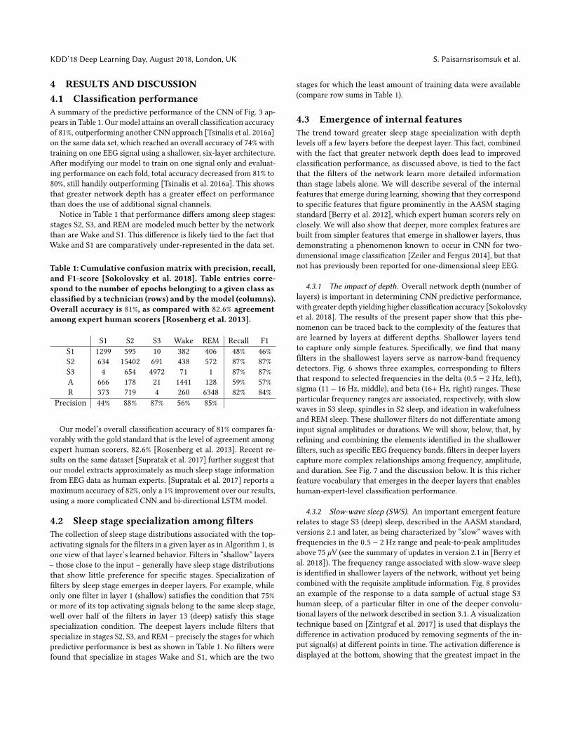
4 RESULTS AND DISCUSSION4.1 Classification performanceA summary of the predictive performance of the CNN of Fig. 3 ap-pears in Table 1. Our model attains an overall classification accuracyof 81%, outperforming another CNN approach [Tsinalis et al. 2016a]on the same data set, which reached an overall accuracy of 74% withtraining on one EEG signal using a shallower, six-layer architecture.After modifying our model to train on one signal only and evaluat-ing performance on each fold, total accuracy decreased from 81% to80%, still handily outperforming [Tsinalis et al. 2016a]. This showsthat greater network depth has a greater effect on performancethan does the use of additional signal channels.

Notice in Table 1 that performance differs among sleep stages:stages S2, S3, and REM are modeled much better by the networkthan are Wake and S1. This difference is likely tied to the fact thatWake and S1 are comparatively under-represented in the data set.

Table 1: Cumulative confusionmatrix with precision, recall,and F1-score [Sokolovsky et al. 2018]. Table entries corre-spond to the number of epochs belonging to a given class asclassified by a technician (rows) and by themodel (columns).Overall accuracy is 81%, as compared with 82.6% agreementamong expert human scorers [Rosenberg et al. 2013].

S1 S2 S3 Wake REM Recall F1S1 1299 595 10 382 406 48% 46%S2 634 15402 691 438 572 87% 87%S3 4 654 4972 71 1 87% 87%A 666 178 21 1441 128 59% 57%R 373 719 4 260 6348 82% 84%

Precision 44% 88% 87% 56% 85%

Our model’s overall classification accuracy of 81% compares fa-vorably with the gold standard that is the level of agreement amongexpert human scorers, 82.6% [Rosenberg et al. 2013]. Recent re-sults on the same dataset [Supratak et al. 2017] further suggest thatour model extracts approximately as much sleep stage informationfrom EEG data as human experts. [Supratak et al. 2017] reports amaximum accuracy of 82%, only a 1% improvement over our results,using a more complicated CNN and bi-directional LSTM model.

4.2 Sleep stage specialization among filtersThe collection of sleep stage distributions associated with the top-activating signals for the filters in a given layer as in Algorithm 1, isone view of that layer’s learned behavior. Filters in “shallow” layers– those close to the input – generally have sleep stage distributionsthat show little preference for specific stages. Specialization offilters by sleep stage emerges in deeper layers. For example, whileonly one filter in layer 1 (shallow) satisfies the condition that 75%or more of its top activating signals belong to the same sleep stage,well over half of the filters in layer 13 (deep) satisfy this stagespecialization condition. The deepest layers include filters thatspecialize in stages S2, S3, and REM – precisely the stages for whichpredictive performance is best as shown in Table 1. No filters werefound that specialize in stages Wake and S1, which are the two

stages for which the least amount of training data were available(compare row sums in Table 1).

4.3 Emergence of internal featuresThe trend toward greater sleep stage specialization with depthlevels off a few layers before the deepest layer. This fact, combinedwith the fact that greater network depth does lead to improvedclassification performance, as discussed above, is tied to the factthat the filters of the network learn more detailed informationthan stage labels alone. We will describe several of the internalfeatures that emerge during learning, showing that they correspondto specific features that figure prominently in the AASM stagingstandard [Berry et al. 2012], which expert human scorers rely onclosely. We will also show that deeper, more complex features arebuilt from simpler features that emerge in shallower layers, thusdemonstrating a phenomenon known to occur in CNN for two-dimensional image classification [Zeiler and Fergus 2014], but thatnot has previously been reported for one-dimensional sleep EEG.

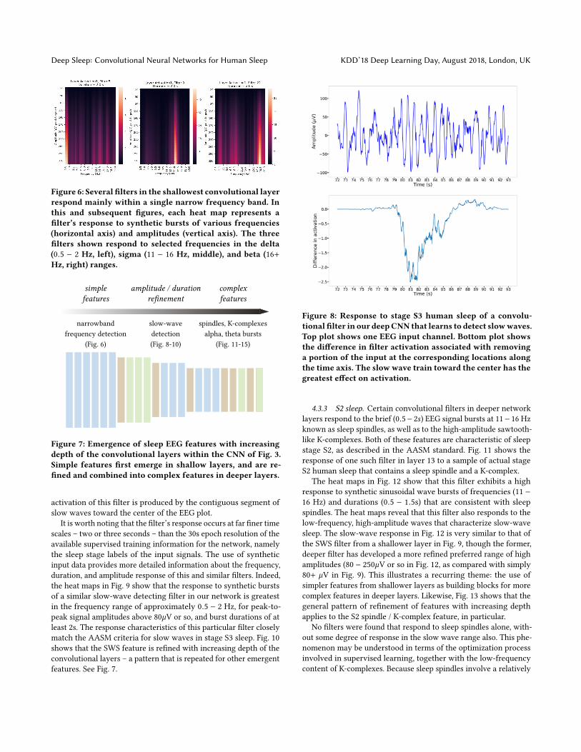
4.3.1 The impact of depth. Overall network depth (number oflayers) is important in determining CNN predictive performance,with greater depth yielding higher classification accuracy [Sokolovskyet al. 2018]. The results of the present paper show that this phe-nomenon can be traced back to the complexity of the features thatare learned by layers at different depths. Shallower layers tendto capture only simple features. Specifically, we find that manyfilters in the shallowest layers serve as narrow-band frequencydetectors. Fig. 6 shows three examples, corresponding to filtersthat respond to selected frequencies in the delta (0.5 − 2 Hz, left),sigma (11 − 16 Hz, middle), and beta (16+ Hz, right) ranges. Theseparticular frequency ranges are associated, respectively, with slowwaves in S3 sleep, spindles in S2 sleep, and ideation in wakefulnessand REM sleep. These shallower filters do not differentiate amonginput signal amplitudes or durations. We will show, below, that, byrefining and combining the elements identified in the shallowerfilters, such as specific EEG frequency bands, filters in deeper layerscapture more complex relationships among frequency, amplitude,and duration. See Fig. 7 and the discussion below. It is this richerfeature vocabulary that emerges in the deeper layers that enableshuman-expert-level classification performance.

4.3.2 Slow-wave sleep (SWS). An important emergent featurerelates to stage S3 (deep) sleep, described in the AASM standard,versions 2.1 and later, as being characterized by “slow” waves withfrequencies in the 0.5 − 2 Hz range and peak-to-peak amplitudesabove 75 µV (see the summary of updates in version 2.1 in [Berry etal. 2018]). The frequency range associated with slow-wave sleepis identified in shallower layers of the network, without yet beingcombined with the requisite amplitude information. Fig. 8 providesan example of the response to a data sample of actual stage S3human sleep, of a particular filter in one of the deeper convolu-tional layers of the network described in section 3.1. A visualizationtechnique based on [Zintgraf et al. 2017] is used that displays thedifference in activation produced by removing segments of the in-put signal(s) at different points in time. The activation difference isdisplayed at the bottom, showing that the greatest impact in the

Deep Sleep: Convolutional Neural Networks for Human Sleep KDD’18 Deep Learning Day, August 2018, London, UK

Figure 6: Several filters in the shallowest convolutional layerrespond mainly within a single narrow frequency band. Inthis and subsequent figures, each heat map represents afilter’s response to synthetic bursts of various frequencies(horizontal axis) and amplitudes (vertical axis). The threefilters shown respond to selected frequencies in the delta(0.5 − 2 Hz, left), sigma (11 − 16 Hz, middle), and beta (16+Hz, right) ranges.

simplefeatures

narrowbandfrequency detection

(Fig. 6)

amplitude / durationrefinement

slow-wavedetection(Fig. 8-10)

complexfeatures

spindles, K-complexesalpha, theta bursts

(Fig. 11-15)

Figure 7: Emergence of sleep EEG features with increasingdepth of the convolutional layers within the CNN of Fig. 3.Simple features first emerge in shallow layers, and are re-fined and combined into complex features in deeper layers.

activation of this filter is produced by the contiguous segment ofslow waves toward the center of the EEG plot.

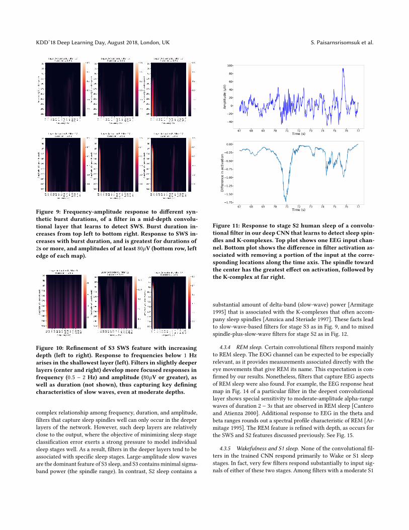
It is worth noting that the filter’s response occurs at far finer timescales – two or three seconds – than the 30s epoch resolution of theavailable supervised training information for the network, namelythe sleep stage labels of the input signals. The use of syntheticinput data provides more detailed information about the frequency,duration, and amplitude response of this and similar filters. Indeed,the heat maps in Fig. 9 show that the response to synthetic burstsof a similar slow-wave detecting filter in our network is greatestin the frequency range of approximately 0.5 − 2 Hz, for peak-to-peak signal amplitudes above 80µV or so, and burst durations of atleast 2s. The response characteristics of this particular filter closelymatch the AASM criteria for slow waves in stage S3 sleep. Fig. 10shows that the SWS feature is refined with increasing depth of theconvolutional layers – a pattern that is repeated for other emergentfeatures. See Fig. 7.

Figure 8: Response to stage S3 human sleep of a convolu-tional filter in our deepCNN that learns to detect slowwaves.Top plot shows one EEG input channel. Bottom plot showsthe difference in filter activation associated with removinga portion of the input at the corresponding locations alongthe time axis. The slow wave train toward the center has thegreatest effect on activation.

4.3.3 S2 sleep. Certain convolutional filters in deeper networklayers respond to the brief (0.5− 2s) EEG signal bursts at 11− 16 Hzknown as sleep spindles, as well as to the high-amplitude sawtooth-like K-complexes. Both of these features are characteristic of sleepstage S2, as described in the AASM standard. Fig. 11 shows theresponse of one such filter in layer 13 to a sample of actual stageS2 human sleep that contains a sleep spindle and a K-complex.

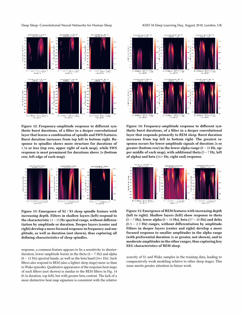
The heat maps in Fig. 12 show that this filter exhibits a highresponse to synthetic sinusoidal wave bursts of frequencies (11 −16 Hz) and durations (0.5 − 1.5s) that are consistent with sleepspindles. The heat maps reveal that this filter also responds to thelow-frequency, high-amplitude waves that characterize slow-wavesleep. The slow-wave response in Fig. 12 is very similar to that ofthe SWS filter from a shallower layer in Fig. 9, though the former,deeper filter has developed a more refined preferred range of highamplitudes (80 − 250µV or so in Fig. 12, as compared with simply80+ µV in Fig. 9). This illustrates a recurring theme: the use ofsimpler features from shallower layers as building blocks for morecomplex features in deeper layers. Likewise, Fig. 13 shows that thegeneral pattern of refinement of features with increasing depthapplies to the S2 spindle / K-complex feature, in particular.

No filters were found that respond to sleep spindles alone, with-out some degree of response in the slow wave range also. This phe-nomenon may be understood in terms of the optimization processinvolved in supervised learning, together with the low-frequencycontent of K-complexes. Because sleep spindles involve a relatively

KDD’18 Deep Learning Day, August 2018, London, UK S. Paisarnsrisomsuk et al.

Figure 9: Frequency-amplitude response to different syn-thetic burst durations, of a filter in a mid-depth convolu-tional layer that learns to detect SWS. Burst duration in-creases from top left to bottom right. Response to SWS in-creases with burst duration, and is greatest for durations of2s or more, and amplitudes of at least 80µV (bottom row, leftedge of each map).

Figure 10: Refinement of S3 SWS feature with increasingdepth (left to right). Response to frequencies below 1 Hzarises in the shallowest layer (left). Filters in slightly deeperlayers (center and right) develop more focused responses infrequency (0.5 − 2 Hz) and amplitude (80µV or greater), aswell as duration (not shown), thus capturing key definingcharacteristics of slow waves, even at moderate depths.

complex relationship among frequency, duration, and amplitude,filters that capture sleep spindles well can only occur in the deeperlayers of the network. However, such deep layers are relativelyclose to the output, where the objective of minimizing sleep stageclassification error exerts a strong pressure to model individualsleep stages well. As a result, filters in the deeper layers tend to beassociated with specific sleep stages. Large-amplitude slow wavesare the dominant feature of S3 sleep, and S3 contains minimal sigma-band power (the spindle range). In contrast, S2 sleep contains a

Figure 11: Response to stage S2 human sleep of a convolu-tional filter in our deep CNN that learns to detect sleep spin-dles and K-complexes. Top plot shows one EEG input chan-nel. Bottom plot shows the difference in filter activation as-sociated with removing a portion of the input at the corre-sponding locations along the time axis. The spindle towardthe center has the greatest effect on activation, followed bythe K-complex at far right.

substantial amount of delta-band (slow-wave) power [Armitage1995] that is associated with the K-complexes that often accom-pany sleep spindles [Amzica and Steriade 1997]. These facts leadto slow-wave-based filters for stage S3 as in Fig. 9, and to mixedspindle-plus-slow-wave filters for stage S2 as in Fig. 12.

4.3.4 REM sleep. Certain convolutional filters respond mainlyto REM sleep. The EOG channel can be expected to be especiallyrelevant, as it provides measurements associated directly with theeye movements that give REM its name. This expectation is con-firmed by our results. Nonetheless, filters that capture EEG aspectsof REM sleep were also found. For example, the EEG response heatmap in Fig. 14 of a particular filter in the deepest convolutionallayer shows special sensitivity to moderate-amplitude alpha-rangewaves of duration 2 − 3s that are observed in REM sleep [Canteroand Atienza 2000]. Additional response to EEG in the theta andbeta ranges rounds out a spectral profile characteristic of REM [Ar-mitage 1995]. The REM feature is refined with depth, as occurs forthe SWS and S2 features discussed previously. See Fig. 15.

4.3.5 Wakefulness and S1 sleep. None of the convolutional fil-ters in the trained CNN respond primarily to Wake or S1 sleepstages. In fact, very few filters respond substantially to input sig-nals of either of these two stages. Among filters with a moderate S1

Deep Sleep: Convolutional Neural Networks for Human Sleep KDD’18 Deep Learning Day, August 2018, London, UK

Figure 12: Frequency-amplitude response to different syn-thetic burst durations, of a filter in a deeper convolutionallayer that learns a combination of spindle and SWS features.Burst duration increases from top left to bottom right. Re-sponse to spindles shows more structure for durations of1.5s or less (top row, upper right of each map), while SWSresponse is most prominent for durations above 2s (bottomrow, left edge of each map).

Figure 13: Emergence of S2 / S3 sleep spindle feature withincreasing depth. Filters in shallow layers (left) respond tothe characteristic 11−15Hz spectral range, without differen-tiation by amplitude or duration. Deeper layers (center andright) develop amore focused response in frequency and am-plitude, as well as duration (not shown), thus capturing alldefining characteristics of sleep spindles.

response, a common feature appears to be a sensitivity to shorter-duration, lower-amplitude bursts in the theta (4 − 7 Hz) and alpha(8 − 12 Hz) spectral bands, as well as the beta band (16+ Hz). Suchfilters also respond to REM (also a lighter sleep stage) more so thantoWake episodes. Qualitative appearance of the response heat mapsof such filters (not shown) is similar to the REM filters in Fig. 14(0.5s duration, top left), but with greater beta content. The lack of amore distinctive heat map signature is consistent with the relative

Figure 14: Frequency-amplitude response to different syn-thetic burst durations, of a filter in a deeper convolutionallayer that responds primarily to REM sleep. Burst durationincreases from top left to bottom right. The greatest re-sponse occurs for lower-amplitude signals of duration 2s orgreater (bottom row) in the lower alpha range (8− 10Hz, up-per middle of each map), with additional theta (5− 7Hz, leftof alpha) and beta (16+ Hz, right end) response.

Figure 15: Emergence ofREM featureswith increasing depth(left to right). Shallow layers (left) show response to theta(5 − 7 Hz), lower alpha (8 − 10 Hz), beta (17 − 20 Hz) and delta(0.5 − 2.5 Hz) ranges, without differentiation by amplitude.Filters in deeper layers (center and right) develop a morefocused response to smaller amplitudes in the alpha range(with preferential duration 2s or greater, not shown), and tomoderate amplitudes in the other ranges, thus capturingkeyEEG characteristics of REM sleep.

scarcity of S1 and Wake samples in the training data, leading tocomparatively weak modeling relative to other sleep stages. Thisissue merits greater attention in future work.

KDD’18 Deep Learning Day, August 2018, London, UK S. Paisarnsrisomsuk et al.

5 CONCLUSIONSWe described our work in predictive modeling in sleep medicineusing a deep convolutional neural network (CNN) architecture forsleep stage classification of multi-channel polysomnogram (PSG)data, together with domain interpretation of the emergent inter-nal features. The classification performance of the proposed CNNmodel is at approximately the same level as the rate of agreementamong human expert scorers, which can reasonably be taken asan upper bound on objectively meaningful performance in thiscontext. We showed that the excellent performance of this modelis due mostly to its depth (17 convolutional layers, with additionalpooling and batch normalization layers), and not to the use of multi-channel data, as using a single EEG channel results in only a minordecrease in classification accuracy (80% vs. 81%).

Using visualization and analysis of network response to nat-ural human sleep data and synthetic burst data, we identifiedspecific emergent EEG features in the convolutional filters of theCNN, including large-amplitude slow waves, sleep spindles andK-complexes, and low-amplitude alpha waves, that human expertsrely on for the visual scoring of sleep. The complexity of the emer-gent features increases with depth within the CNN. Many filtersin shallow layers act as narrowband frequency detectors. Deeperlayers refine and combine the more elementary features to capturepatterns that are representative of individual sleep stages. For ex-ample, an emerging slow-wave feature is refined in deeper layersto account for a preferred range of amplitudes. Other convolutionalfilters in deep layers respond sensitively to both sleep spindles andK-complexes – features that co-occur in sleep stage S2. Yet otherfilters respond to the alpha bursts that occur in REM sleep. Thispaper provides an important new demonstration of hierarchicalfeature emergence in CNN for physiological time series data, thefirst such work that we are aware of in sleep stage classification.

ACKNOWLEDGMENTSThe authors thank Majaz Moonis, M.D., of the U. of Mass. MedicalSchool, for helpful conversations on polysomnography and sleep.

REFERENCESMartín Abadi, Ashish Agarwal, Paul Barham, Eugene Brevdo, Zhifeng Chen, Craig

Citro, Greg S Corrado, Andy Davis, Jeffrey Dean, Matthieu Devin, et al. 2016.TensorFlow: Large-scale machine learning on heterogeneous distributed systems.arXiv preprint arXiv:1603.04467 (2016).

Florin Amzica andMircea Steriade. 1997. The K-complex: Its slow (< 1-Hz) rhythmicityand relation to delta waves. Neurology 49, 4 (1997), 952–959. https://doi.org/10.1212/WNL.49.4.952 arXiv:http://n.neurology.org/content/49/4/952.full.pdf

R. Armitage. 1995. The distribution of EEG frequencies in REM and NREM sleep stagesin healthy young adults. Sleep 18, 5 (June 1995), 334–341.

Richard B Berry, Rita Brooks, Charlene E Gamaldo, Susan M Harding, CL Marcus,and BV Vaughn. 2012. The AASM manual for the scoring of sleep and associatedevents. Rules, Terminology and Technical Specifications. American Academy ofSleep Medicine (2012).

Richard B Berry et al. 2018. (Updates to) The AASMManual for the Scoring of Sleep andAssociated Events. (2018). https://aasm.org/clinical-resources/scoring-manual/

José Luis Cantero and Mercedes Atienza. 2000. Alpha burst activity during humanREM sleep: descriptive study and functional hypotheses. Clinical Neurophysiology111, 5 (2000), 909 – 915. https://doi.org/10.1016/S1388-2457(99)00318-1

Xudong Cao. [n. d.]. A practical theory for designing very deep convolu-tional neural networks. ([n. d.]). https://kaggle2.blob.core.windows.net/forum-message-attachments/69182/2287/A%20practical%20theory%20for%20designing%20very%20deep%20convolutional%20neural%20networks.pdf

François Chollet et al. 2015. Keras. https://keras.io. (2015).Sander Dieleman and Benjamin Schrauwen. 2014. End-to-end learning for music

audio. In Acoustics, Speech and Signal Processing (ICASSP), 2014 IEEE International

Conference on. IEEE, 6964–6968.D. Gabor. 1946. Theory of communication. Part 1: The analysis of information. Electrical

Engineers - Part III: Radio and Communication Engineering, Journal of the Institutionof 93, 26 (November 1946), 429–441. https://doi.org/10.1049/ji-3-2.1946.0074

AL Goldberger, LANAmaral, L Glass, JMHausdorff, PC Ivanov, RGMark, JEMietus, GBMoody, C-K Peng, and HE Stanley. 2000. Physiobank, physiotoolkit, and physionet.Circulation 101, 23 (2000), e215–e220.

Ian Goodfellow, Yoshua Bengio, and Aaron Courville. 2016. Deep Learning. MIT Press.http://www.deeplearningbook.org.

Madeleine M Grigg-Damberger. 2009. The AASM scoring manual: a critical appraisal.Current opinion in pulmonary medicine 15, 6 (2009), 540–549.

Kaiming He, Xiangyu Zhang, Shaoqing Ren, and Jian Sun. 2015. Delving deep intorectifiers: Surpassing human-level performance on imagenet classification. In Pro-ceedings of the IEEE international conference on computer vision. 1026–1034.

Sergey Ioffe and Christian Szegedy. 2015. Batch normalization: Accelerating deep net-work training by reducing internal covariate shift. arXiv preprint arXiv:1502.03167(2015).

Eric Kauderer-Abrams. 2018. Quantifying Translation-Invariance in ConvolutionalNeural Networks. CoRR abs/1801.01450 (2018). arXiv:1801.01450 http://arxiv.org/abs/1801.01450

B Kemp, AH Zwinderman, B Tuk, HAC Kamphuisen, and JJL Oberyé. 2000. Analysisof a sleep-dependent neuronal feedback loop: the slow-wave microcontinuity ofthe EEG. IEEE-BME 47, 9 (2000), 1185–1194.

Serkan Kiranyaz, Turker Ince, and Moncef Gabbouj. 2016. Real-time patient-specificECG classification by 1-D convolutional neural networks. IEEE Transactions onBiomedical Engineering 63, 3 (2016), 664–675.

Alex Krizhevsky, Ilya Sutskever, and Geoffrey E Hinton. 2012. Imagenet classifica-tion with deep convolutional neural networks. In Advances in neural informationprocessing systems. 1097–1105.

Martin Längkvist, Lars Karlsson, and Amy Loutfi. 2012. Sleep stage classification usingunsupervised feature learning. Advances in Artificial Neural Systems 2012 (2012).https://doi.org/doi:10.1155/2012/107046

G. Medic, M. Wille, and M. E. Hemels. 2017. Short- and long-term health consequencesof sleep disruption. Nature and Science of Sleep 9 (2017), 151–161. https://doi.org/10.2147/NSS.S134864

Karol J Piczak. 2015. Environmental sound classification with convolutional neu-ral networks. In Machine Learning for Signal Processing (MLSP), 2015 IEEE 25thInternational Workshop on. IEEE, 1–6.

Waseem Rawat and Zenghui Wang. 2017. Deep Convolutional Neural Networks forImage Classification: A Comprehensive Review. Neural Comput. 29, 9 (Sept. 2017),2352–2449. https://doi.org/10.1162/neco_a_00990

Shaoqing Ren, Kaiming He, Ross Girshick, and Jian Sun. 2015. Faster R-CNN: Towardsreal-time object detection with region proposal networks. In Advances in neuralinformation processing systems. 91–99.

Marco Roessen and Bob Kemp. 2018. Polyman EDF+ viewer. (2018). http://www.edfplus.info

Richard S Rosenberg, Steven Van Hout, et al. 2013. The American Academy of SleepMedicine inter-scorer reliability program: sleep stage scoring. J Clin Sleep Med 9, 1(2013), 81–87.

Michael H Silber, Sonia Ancoli-Israel, Michael H Bonnet, Sudhansu Chokroverty,Madeleine M Grigg-Damberger, Max Hirshkowitz, Sheldon Kapen, Sharon AKeenan, Meir H Kryger, Thomas Penzel, et al. 2007. The visual scoring of sleep inadults. J Clin Sleep Med 3, 2 (2007), 121–131.

Karen Simonyan and Andrew Zisserman. 2014. Very deep convolutional networks forlarge-scale image recognition. arXiv preprint arXiv:1409.1556 (2014).

M. Sokolovsky, F. Guerrero, S. Paisarnsrisomsuk, C. Ruiz, and S.A. Alvarez. 2018.Human expert-level automated sleep stage prediction and feature discovery bydeep convolutional neural networks. BIOKDD 2018 (2018).

Akara Supratak, Hao Dong, Chao Wu, and Yike Guo. 2017. DeepSleepNet: a Model forAutomatic Sleep Stage Scoring based on Raw Single-Channel EEG. IEEE Transactionson Neural Systems and Rehabilitation Engineering 25 (2017), 1998–2008.

Orestis Tsinalis, Paul M Matthews, and Yike Guo. 2016a. Automatic sleep stagescoring using time-frequency analysis and stacked sparse autoencoders. Annals ofbiomedical engineering 44, 5 (2016), 1587–1597.

Orestis Tsinalis, Paul M Matthews, Yike Guo, and Stefanos Zafeiriou. 2016b. Auto-matic Sleep Stage Scoring with Single-Channel EEG Using Convolutional NeuralNetworks. arXiv preprint arXiv:1610.01683 (2016).

Jason Yosinski, Jeff Clune, Anh Nguyen, Thomas Fuchs, and Hod Lipson. 2015. Under-standing Neural Networks Through Deep Visualization. In Deep Learning Workshop,International Conference on Machine Learning (ICML).

Matthew D Zeiler and Rob Fergus. 2014. Visualizing and understanding convolutionalnetworks. In European Conference on Computer Vision (ECCV). Springer, 818–833.

Haomin Zhang, Ian McLoughlin, and Yan Song. 2015. Robust sound event recognitionusing convolutional neural networks. In Acoustics, Speech and Signal Processing(ICASSP), 2015 IEEE International Conference on. IEEE, 559–563.

Luisa M. Zintgraf, Taco S. Cohen, Tameem Adel, and Max Welling. 2017. Visual-izing Deep Neural Network Decisions: Prediction Difference Analysis. CoRRabs/1702.04595 (2017). arXiv:1702.04595 http://arxiv.org/abs/1702.04595