1

1

Deep Multi-Scale Resemblance Network for the Sub-class

Differentiation of Adrenal Masses on Computed Tomography Images

Lei Bia,*, Jinman Kim a,*, Tingwei Sub, Michael Fulhama,c,d, David Dagan Fenga,e, and, Guang Ningb

a School of Computer Science, University of Sydney, NSW, Australia

b Department of Endocrine and Metabolic Diseases, Ruijin Hospital, Shanghai Jiao Tong University School of

Medicine, Shanghai, China

c Department of Molecular Imaging, Royal Prince Alfred Hospital, NSW, Australia

d Sydney Medical School, University of Sydney, NSW, Australia

e Med-X Research Institute, Shanghai Jiao Tong University, Shanghai, China

* Corresponding author: lei.bi@sydney.edu.au; jinman.kim@sydney.edu.au

Abstract — Objective: The accurate classification of mass lesions in the adrenal glands (‘adrenal masses’), detected

with computed tomography (CT), is important for diagnosis and patient management. Adrenal masses can be benign

or malignant and the benign masses have varying prevalence. Classification methods based on convolutional neural

networks (CNN) are the state-of-the-art in maximizing inter-class differences in large medical imaging training

datasets. The application of CNNs, to adrenal masses is challenging due to large intra-class variations, large inter-

class similarities and imbalanced training data due to the size of masses. Methods: We developed a deep multi-scale

resemblance network (DMRN) to overcome these limitations and leveraged paired CNNs to evaluate the intra-class

similarities. We used multi-scale feature embedding to improve the inter-class separability by iteratively combining

complementary information produced at different scales of the input to create structured feature descriptors. We also

augmented the training data with randomly sampled paired adrenal masses to reduce the influence of imbalanced

2

2

training data. We used 229 CT scans of patients with adrenal masses. Results: Our method had the best results

compared to state-of-the-art methods. Conclusion: Our DMRN sub-classified adrenal masses on CT and was superior

to state-of-the-art approaches.

Keywords — Classification, Adrenal Masses, Convolutional Neural Networks (CNN)

1. INTRODUCTION

There are a large variety of abnormalities that are detected in the adrenal glands on abdominal / lower thoracic

computed tomography (CT) scans. These abnormalities range from benign cystic changes / calcification to high grade

malignant tumors that may arise in the gland itself (primary tumors) or reflect metastatic disease from another site e.g.

a primary lung, bowel or skin cancer. The prevalence of mass lesions in the adrenal glands (‘adrenal masses’) is

unclear but it has been suggested that the prevalence of adrenal adenomas, a sub-class of benign primary tumors, is

7% in subjects over 70 years of age [1]. Adrenal masses can be asymptomatic but there are a number of well-described

clinical syndromes that are associated with tumors that secrete an excess amount of adrenal hormones such as cortisol,

aldosterone, norepinephrine etc. [2-4]. An imaging specialist uses characteristics such as size, shape, homogeneity,

morphology, density, presence of fat / calcification and characteristics of contrast enhancement on CT to sub-classify

adrenal masses. There are large intra-class variations and large inter-class similarities between the various adrenal

masses. The visual distinction between different classes can be subtle and texture variations within the same sub-

classes can be marked. Thus assessment requires an experienced reader and pose challenges for less experienced

imaging specialists and clinicians. Prior studies suggest that an automated computer aided diagnosis system (CAD)

could improve accuracy and reduce image reading time [5, 6]. Hence our aim was to explore the possibility of

developing an automated process to sub-classify adrenal masses that are assessed by a large endocrine service. The

main sub-classes of adrenal masses are: (i) adrenocortical carcinomas (ACAs); (ii) non-functional adrenal adenomas

(NAAs); (iii) ganglioneuromas (GAs); (iv) adrenal myelolipomas (AMs); and (v) pheochromocytomas (PCCs). These

adrenal masses vary in prevalence and adenomas are very common as outlined above and carcinomas are rare. The

normal adrenal glands are usually located in the posterior upper abdomen, antero-superior to the upper pole of each

kidney. In Fig. 1 we show paired transaxial image CT slices of typical examples to illustrate the heterogeneity across

and, within, these adrenal masses. There are differences in shape, density and patterns of contrast enhancement. AMs

3

3

have a mixed soft tissue and fat density, vary in size and do not enhance. The varying size of different adrenal masses

means that any training characteristics will be imbalanced. Existing classification methods tend to overfit to sub-

classes with a large number of training characteristics and perform poorly on other sub-classes.

Figure 1. Paired transaxial contrast-enhanced CT images of different adrenal masses (red arrows).

1.1. Related Work

Current automated medical imaging classification methods are: (i) traditional, using handcrafted features, with

conventional classifiers; and (ii) deep learning using deep convolutional neural networks (CNNs). In traditional

methods handcrafted techniques encode image characteristics as the feature descriptors and label image categories

with supervised approaches. The most commonly used features include the local binary pattern (LBP) [6, 7], histogram

of oriented gradients (HOG) [6, 8], gray level co-occurrence matrix (GLCM) and run length-based (RLE) texture [9-

13] and wavelets [14, 15]. The extracted visual features train classifiers such as the support vector machine (SVM) [6,

8, 16, 17], K-nearest neighbor (KNN) [7, 18, 19] and random forest (RF) [14, 20-22]. Their performance, however,

depends on effective pre-processing to reduce noise, tune a large number of parameters and manipulate the hand-

crafted features and this limits their generalizability.

Deep learning uses CNNs to leverage large datasets to learn the features that best correspond to the appearance /

semantics of the images [23]. CNNs can be trained in an end-to-end manner for efficient inference, i.e., images are

taken as inputs and classification results are directly outputted. Anthimopoulos et al used a CNN with 5 convolutional

4

4

layers to classify interstitial lung disease on chest CT [24]. Dou et al reported a cascaded 3D CNN to detect

microbleeds on Magnetic Resonance (MR) scans [25]. Standard CNNs have difficulties when there are large intra-

class variations, large inter-class similarities and imbalanced data [26, 27].

Many researchers have attempted to solve the problem of imbalanced data through augmenting the training dataset

with additional image features or CNNs. Zhen et al proposed augmentation with Fisher features for melanoma

detection on dermoscopy images [28]. Ahn et al leveraged pre-trained Visual Geometry Group (VGG) network

features (trained on natural images e.g., ImageNet) with scale-invariant feature transforms [29]. Wang et al reported

a multiscale rotation-invariant CNN with Gabor features for lung texture classification on chest CT [26]. Kumar et al

used a combination of features from multiple CNNs to alleviate the problem of imbalanced data [30]. Augmentation

methods balance the data distribution by duplicating existing training features, but they do not produce new features

for learning.

A number of researchers have modeled the inter-class differences to manage large intra-class variations and inter-

class similarities in image datasets. Zhang et al trained multiple CNNs in a competitive manner to learn differences in

the input data from different classes [27]. Ahn et al employed a convolutional sparse kernel network to learn class-

specific image features for better discrimination [31]. Zhang et al proposed an attention residual learning network to

learn subtle inter-class image features [32]. All these methods were designed to learn inter-class differences through

maximizing inter-class distances, without minimizing large intra-class variations. Hence, they are less effective for

images with large intra-class variations.

1.2. Our Contribution

We suggest a different approach to differentiate adrenal masses on CT and our contribution is as follows:

(1) We proposed a similarity loss to derive features that was able to tolerate large intra-class variations. We

leveraged paired CNNs to evaluate the intra-class feature differences and then used the similarity loss to gradually

learn the intra-class training samples with large feature distances.

(2) We proposed a multi-scale feature embedding to refine feature learning. We progressively integrated the

complementary feature representations produced at different scales (levels) of the input adrenal masses to create

structured feature descriptors that then to improve the discriminating power for sub-class classification.

(3) We leveraged paired inputs to ameliorate imbalanced training data by augmenting the training data with

5

5

randomly sampled data from different sub-classes to create the paired data. Thus all sub-classes have equal

contributions to the final model and the risk of overfitting is minimized.

In the rest of the paper we have Methods and Evaluation in Section 2, Results in Section 3, Discussion in Section 4

and Conclusions in Section 5.

2. METHODS

2.1. Materials

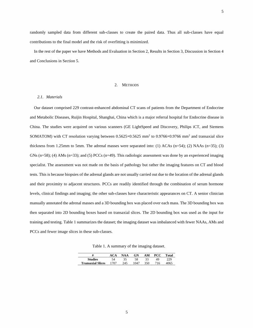
Our dataset comprised 229 contrast-enhanced abdominal CT scans of patients from the Department of Endocrine

and Metabolic Diseases, Ruijin Hospital, Shanghai, China which is a major referral hospital for Endocrine disease in

China. The studies were acquired on various scanners (GE LightSpeed and Discovery, Philips iCT, and Siemens

SOMATOM) with CT resolution varying between 0.5625×0.5625 mm2 to 0.9766×0.9766 mm2 and transaxial slice

thickness from 1.25mm to 5mm. The adrenal masses were separated into: (1) ACAs (n=54); (2) NAAs (n=35); (3)

GNs (n=58); (4) AMs (n=33); and (5) PCCs (n=49). This radiologic assessment was done by an experienced imaging

specialist. The assessment was not made on the basis of pathology but rather the imaging features on CT and blood

tests. This is because biopsies of the adrenal glands are not usually carried out due to the location of the adrenal glands

and their proximity to adjacent structures. PCCs are readily identified through the combination of serum hormone

levels, clinical findings and imaging; the other sub-classes have characteristic appearances on CT. A senior clinician

manually annotated the adrenal masses and a 3D bounding box was placed over each mass. The 3D bounding box was

then separated into 2D bounding boxes based on transaxial slices. The 2D bounding box was used as the input for

training and testing. Table 1 summarizes the dataset; the imaging dataset was imbalanced with fewer NAAs, AMs and

PCCs and fewer image slices in these sub-classes.

Table 1. A summary of the imaging dataset.

# ACA NAA GN AM PCC Total

Studies 54 35 58 33 49 229 Transaxial Slices 1707 245 1047 350 716 4065

6

6

2.2. Deep Multi-Scale Resemblance Network (DMRN)

Figure 2. Flow diagram of our deep multi-scale resemblance network (DMRN)

A flow diagram of our method based on ResNet backbone is shown in Fig. 2. We applied ResNet to the paired

training images (randomly produced) to generate feature maps at various scales. The feature maps from each scale

were then embedded into paired feature vectors 𝑥1and 𝑥2 via the residual pooling unit (RPU). Then the similarity

feature learning module measured the similarities between the two feature vectors at different scales and was trained

to determine if the two feature vectors were from the same class (𝑌 = 0 if 𝑥1and 𝑥2 were from same class, and 𝑌 = 1

if they were from different classes).

2.2.1. Multi-Scale Feature Embedding

A ResNet was used as the backbone for the initial design for its wide applications and scalability [33, 34]. The

ResNet architecture has a number of residual blocks and a residual block utilizes a skip connection to bypass a few

convolutional, batch normalization and rectified linear unit (ReLUs) layers at a time. The use of skip connections

enables to reuse the activations from a previous layer (previous residual block) which thereby minimizes the problem

of vanishing gradients.

Our ResNet has 4 stages representing 4 different feature maps - 56×56, 28×28, 14×14, and 7×7. For the output

7

7

feature maps, we used an RPU to pool 2D feature maps into a single 1D feature vector and to pool spatial and semantic

features at that stage. The RPUs start with two convolutional layers - a ReLU and summation layers with a kernel size

of 3×3, which is a simplified version of the residual block in the original ResNet, where the batch normalization layers

were removed. We applied an adaptive average pooling operation to aggregate the spatial information within the

feature maps, where we used adaptive average pooling to the summed feature maps to down-sample the feature maps

into 1×1. At the final stage of the RPU, we used a fully connected layer (FC) to use the inter-channel relationship and

to reduce parameter overhead, where the output of the FC has been set to 25% of the input in size.

2.2.2. Similarity Feature Learning

Our similarity feature learning module learns subtle feature differences of the paired inputs at individual stages. Let

𝑥1𝑡, 𝑥2

𝑡 be a pair of feature vectors derived from the fully connected layer of the two RPUs at stage 𝑡. Let 𝑌 be a binary

label assigned to this pair, where 𝑌 = 0 if 𝑥1𝑡 and 𝑥2

𝑡 are from same adrenal mass sub-class, and 𝑌 = 1 if they are from

different adrenal mass sub-classes. 𝐷𝑡 is the parameterized distance function of 𝑥1𝑡 and 𝑥2

𝑡 , which is defined as:

𝐷𝑡(𝑥1𝑡 , 𝑥2

𝑡 , 𝜽) = ‖(𝑥1𝑡) − (𝑥2

𝑡)‖2 (1)

Where 𝜽 represents the network parameters. Then the overall loss function across all the stages is to find an optimal

𝜽 can satisfy the following:

ℒ = 𝑎𝑟𝑔min𝜽

∑ ∑ 𝐿𝑡(𝜽, (𝑌, 𝑥1𝑡 , 𝑥2

𝑡)𝑖)𝑃𝑖=1

𝑇𝑡=1 (2)

Where 𝑖 represents the 𝑖 -th training pair out of 𝑃 training sample pairs and 𝑇 represents different stages.

𝐿𝑡(𝜽, (𝑌, 𝑥1𝑡 , 𝑥2

𝑡)) can be defined as:

𝐿𝑡(𝜽, (𝑌, 𝑥1𝑡 , 𝑥2

𝑡)) = (1 − 𝑌)𝐿𝑆𝑡 (𝐷𝑡) + 𝑌𝐿𝐷

𝑡 (𝐷𝑡) (3)

𝐿𝑆𝑡 represents the similarity loss and 𝐿𝐷

𝑡 is the dissimilarity loss, which are defined as:

𝐿𝑆𝑡 =

1

2(𝐷𝑡(𝑥1

𝑡 , 𝑥2𝑡 , 𝜽))2 (4)

𝐿𝐷𝑡 =

1

2{max(0,𝑚 − 𝐷𝑡(𝑥1

𝑡 , 𝑥2𝑡 , 𝜽)}2 (5)

where 𝑚 is a margin threshold and defines when the 𝑥1𝑡 and 𝑥2

𝑡 from different sub-classes will contribute to the loss.

Based on the work proposed by Hadsell et al [35], we set 𝑚 = 1.

8

8

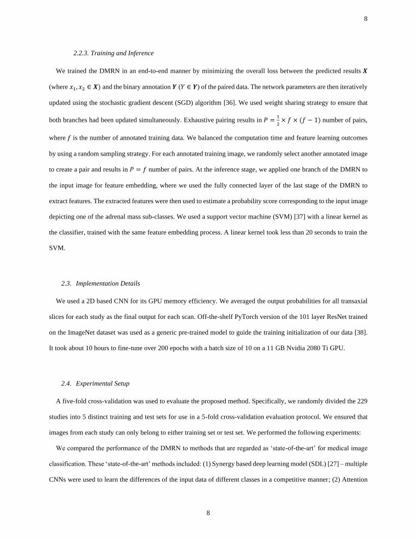
2.2.3. Training and Inference

We trained the DMRN in an end-to-end manner by minimizing the overall loss between the predicted results 𝑿

(where 𝑥1, 𝑥2 ∈ 𝑿) and the binary annotation 𝒀 (𝑌 ∈ 𝒀) of the paired data. The network parameters are then iteratively

updated using the stochastic gradient descent (SGD) algorithm [36]. We used weight sharing strategy to ensure that

both branches had been updated simultaneously. Exhaustive pairing results in 𝑃 =1

2× 𝑓 × (𝑓 − 1) number of pairs,

where 𝑓 is the number of annotated training data. We balanced the computation time and feature learning outcomes

by using a random sampling strategy. For each annotated training image, we randomly select another annotated image

to create a pair and results in 𝑃 = 𝑓 number of pairs. At the inference stage, we applied one branch of the DMRN to

the input image for feature embedding, where we used the fully connected layer of the last stage of the DMRN to

extract features. The extracted features were then used to estimate a probability score corresponding to the input image

depicting one of the adrenal mass sub-classes. We used a support vector machine (SVM) [37] with a linear kernel as

the classifier, trained with the same feature embedding process. A linear kernel took less than 20 seconds to train the

SVM.

2.3. Implementation Details

We used a 2D based CNN for its GPU memory efficiency. We averaged the output probabilities for all transaxial

slices for each study as the final output for each scan. Off-the-shelf PyTorch version of the 101 layer ResNet trained

on the ImageNet dataset was used as a generic pre-trained model to guide the training initialization of our data [38].

It took about 10 hours to fine-tune over 200 epochs with a batch size of 10 on a 11 GB Nvidia 2080 Ti GPU.

2.4. Experimental Setup

A five-fold cross-validation was used to evaluate the proposed method. Specifically, we randomly divided the 229

studies into 5 distinct training and test sets for use in a 5-fold cross-validation evaluation protocol. We ensured that

images from each study can only belong to either training set or test set. We performed the following experiments:

We compared the performance of the DMRN to methods that are regarded as ‘state-of-the-art’ for medical image

classification. These ‘state-of-the-art’ methods included: (1) Synergy based deep learning model (SDL) [27] – multiple

CNNs were used to learn the differences of the input data of different classes in a competitive manner; (2) Attention

9

9

residual learning network (ARL) [32] – ARL uses attention module to focus on learning subtle inter-class image

features; (3) VGG [39] – A 19 layer VGG network; (4) HC – traditional handcrafted features (HC) with SVMs for

classification and we followed existing methods [6] to use LBP and HOG features as the HCs. We used a patch size

of 64 for LBP feature and a patch size of 32 for HOG feature. This resulted in a 531-d LBP feature and a 1296-d HOG

feature. The extracted LBP and HOGs were concatenated into a single feature vector and were then used for

classification; (5) 3D-CNN – A 3 dimensional convolutional neural network (3D-CNN). A similar approach was

proposed by Dou et al [25] for microbleed detection on MR images. We used 6×3D convolutional layers followed by

3 fully connected layers with cross-entropy loss for classification. We also added 3D batch normalization layers and

ReLU layers after each 3D convolutional layers; and (6) ResNet-50, ResNet-101, and ResNet-152 – ResNet with 50,

101 and 152 layers [33].

We further conducted ablation experiments to evaluate the contributions from our method’s individual components.

2.5. Evaluation Metrics

We used the commonly used evaluation metrices including: accuracy (Acc.), sensitivity (Sen.), specificity (Spe.),

precision (Pre.) and F1 score (F1).

𝐴𝑐𝑐. =|𝑇𝑃|+|𝑇𝑁|

|𝑇𝑃|+|𝑇𝑁|+|𝐹𝑃|+|𝐹𝑁| (6)

𝑆𝑒𝑛. =|𝑇𝑃|

|𝑇𝑃|+|𝐹𝑁| (7)

𝑆𝑝𝑒𝑐. =|𝑇𝑁|

|𝑇𝑁|+|𝐹𝑃| (8)

𝑃𝑟𝑒. =|𝑇𝑃|

|𝑇𝑃|+|𝐹𝑃| (9)

𝐹1 =2∙|𝑇𝑃|

2∙|𝑇𝑃|+|𝐹𝑃|+|𝐹𝑁| (10)

where TP is the true positive, TN is the true negative, FN is the false negative and FP is the false positive. All the

evaluation metrics were calculated for individual classes as a one-versus-all approach except for accuracy.

10

10

3. RESULTS

3.1. Classification

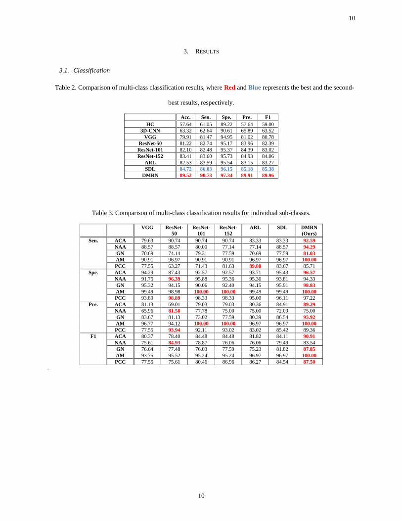
Table 2. Comparison of multi-class classification results, where Red and Blue represents the best and the second-

best results, respectively.

Acc. Sen. Spe. Pre. F1

HC 57.64 61.05 89.22 57.64 59.00

3D-CNN 63.32 62.64 90.61 65.89 63.52

VGG 79.91 81.47 94.95 81.02 80.78

ResNet-50 81.22 82.74 95.17 83.96 82.39

ResNet-101 82.10 82.48 95.37 84.39 83.02

ResNet-152 83.41 83.60 95.73 84.93 84.06

ARL 82.53 83.59 95.54 83.15 83.27

SDL 84.72 86.03 96.15 85.18 85.38

DMRN 89.52 90.73 97.34 89.91 89.96

Table 3. Comparison of multi-class classification results for individual sub-classes.

VGG ResNet-

50

ResNet-

101

ResNet-

152

ARL SDL DMRN

(Ours)

Sen. ACA 79.63 90.74 90.74 90.74 83.33 83.33 92.59

NAA 88.57 88.57 80.00 77.14 77.14 88.57 94.29

GN 70.69 74.14 79.31 77.59 70.69 77.59 81.03

AM 90.91 96.97 90.91 90.91 96.97 96.97 100.00

PCC 77.55 63.27 71.43 81.63 89.80 83.67 85.71

Spe. ACA 94.29 87.43 92.57 92.57 93.71 95.43 96.57

NAA 91.75 96.39 95.88 95.36 95.36 93.81 94.33

GN 95.32 94.15 90.06 92.40 94.15 95.91 98.83

AM 99.49 98.98 100.00 100.00 99.49 99.49 100.00

PCC 93.89 98.89 98.33 98.33 95.00 96.11 97.22

Pre. ACA 81.13 69.01 79.03 79.03 80.36 84.91 89.29

NAA 65.96 81.58 77.78 75.00 75.00 72.09 75.00

GN 83.67 81.13 73.02 77.59 80.39 86.54 95.92

AM 96.77 94.12 100.00 100.00 96.97 96.97 100.00

PCC 77.55 93.94 92.11 93.02 83.02 85.42 89.36

F1 ACA 80.37 78.40 84.48 84.48 81.82 84.11 90.91

NAA 75.61 84.93 78.87 76.06 76.06 79.49 83.54

GN 76.64 77.48 76.03 77.59 75.23 81.82 87.85

AM 93.75 95.52 95.24 95.24 96.97 96.97 100.00

PCC 77.55 75.61 80.46 86.96 86.27 84.54 87.50

.

11

11

Figure 3. Classification results of 4 example CT studies (first row) with varying adrenal masses (columns) using

different methods (second row). Red arrows indicate tumor locations, and color bars correspond to the probabilities

derived from different methods for predicting individual sub-classes.

Table 2 shows the overall results and Table 3 details the results on individual sub-classes. Both Tables show that

the DMRN had the best overall performance across all the measurements and outperformed the second-best method

with >4% in accuracy. Fig. 3 shows classification results of randomly selected challenging studies with classification

probabilities (confidence). It shows that the DMRN was the only method that produced the correct classification with

the highest confidence.

3.2. Component Analysis

We outline the results from individual stage of the DMRN in Table 4. Fig. 4 depicts the classification performance

on individual classes. We note that when coupling multi-scale feature embedding (MS) with similarity feature

learning, the feature representations have been greatly enhanced for differentiation, which resulted in higher

classification accuracy.

Table 4. Classification accuracy comparing with and without multi-scale feature embedding.

Acc. Sen. Spe. Pre. F1

DMRN (w.o. MS) 87.77 88.41 96.92 88.10 88.12

DMRN 89.52 90.73 97.34 89.91 89.96

12

12

Figure 4. Confusion matrix of the classification results compared with and without multi-scale feature embedding.

3.3. Classification Results Analysis

Fig. 5 is the feature visualization results derived using the t-SNE (t-distributed stochastic neighbor embedding)

toolbox [40]. Image features were extracted from transaxial slices. t-SNE uses a nonlinear dimensionality reduction

technique for visualizing high-dimensional image features in a low-dimensional space, and this can be used to indicate

affinities (relationships) among different classes. Compared with ResNet-101, features derived from our DMRN

method presents a clear separation of different sub-classes in t-SNE visualization. Furthermore, ResNet-101 tends to

overfit to the dominant classes while performing poorly on the rest of classes, such as the NAA and AM classes. In

contrast, our method can retain a consistent classification results across different classes.

Figure 5. Feature embedding from (a) ResNet-101; and (b) our DMRN methods, with t-SNE toolbox. Different color

corresponds to different adrenal mass sub-classes. Features were extracted from transaxial slices.

13

13

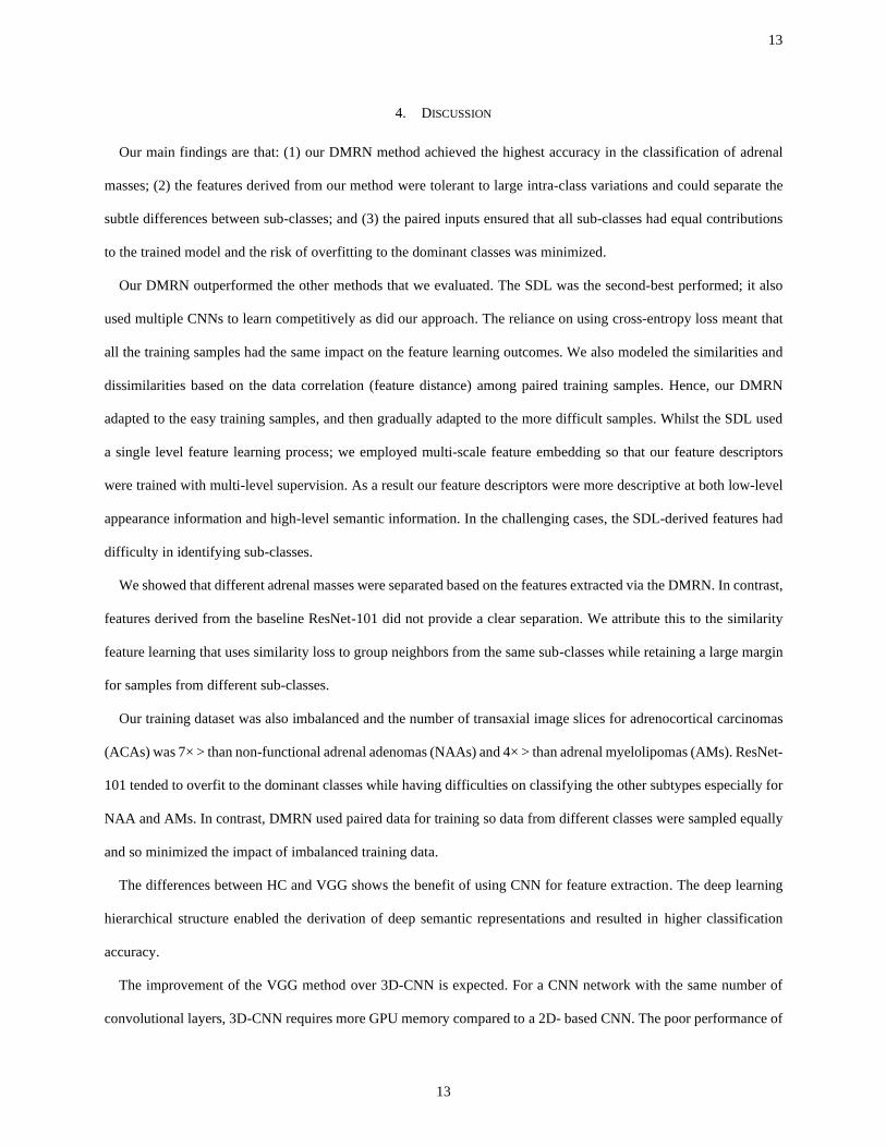
4. DISCUSSION

Our main findings are that: (1) our DMRN method achieved the highest accuracy in the classification of adrenal

masses; (2) the features derived from our method were tolerant to large intra-class variations and could separate the

subtle differences between sub-classes; and (3) the paired inputs ensured that all sub-classes had equal contributions

to the trained model and the risk of overfitting to the dominant classes was minimized.

Our DMRN outperformed the other methods that we evaluated. The SDL was the second-best performed; it also

used multiple CNNs to learn competitively as did our approach. The reliance on using cross-entropy loss meant that

all the training samples had the same impact on the feature learning outcomes. We also modeled the similarities and

dissimilarities based on the data correlation (feature distance) among paired training samples. Hence, our DMRN

adapted to the easy training samples, and then gradually adapted to the more difficult samples. Whilst the SDL used

a single level feature learning process; we employed multi-scale feature embedding so that our feature descriptors

were trained with multi-level supervision. As a result our feature descriptors were more descriptive at both low-level

appearance information and high-level semantic information. In the challenging cases, the SDL-derived features had

difficulty in identifying sub-classes.

We showed that different adrenal masses were separated based on the features extracted via the DMRN. In contrast,

features derived from the baseline ResNet-101 did not provide a clear separation. We attribute this to the similarity

feature learning that uses similarity loss to group neighbors from the same sub-classes while retaining a large margin

for samples from different sub-classes.

Our training dataset was also imbalanced and the number of transaxial image slices for adrenocortical carcinomas

(ACAs) was 7× > than non-functional adrenal adenomas (NAAs) and 4× > than adrenal myelolipomas (AMs). ResNet-

101 tended to overfit to the dominant classes while having difficulties on classifying the other subtypes especially for

NAA and AMs. In contrast, DMRN used paired data for training so data from different classes were sampled equally

and so minimized the impact of imbalanced training data.

The differences between HC and VGG shows the benefit of using CNN for feature extraction. The deep learning

hierarchical structure enabled the derivation of deep semantic representations and resulted in higher classification

accuracy.

The improvement of the VGG method over 3D-CNN is expected. For a CNN network with the same number of

convolutional layers, 3D-CNN requires more GPU memory compared to a 2D- based CNN. The poor performance of

14

14

the 3D-CNN was likely due to the limited size of the GPU memory which restricted the number of convolutional

layers to be inserted into the 3D networks. Consequently, the learned features from the 3D-CNN will be sub-optimal

for differentiating the different adrenal masses.

The improvement of ResNet when compared to the VGG, we suggest, is likely to be due to using residual blocks

that allowed an increase in the overall depth of the network. When compared with ResNet based methods such as

ResNet-50 and ResNet-101, ARL showed a marginal 1% improvement in accuracy. ARL uses an attention module to

focus on subtle inter-class features which minimizes the problem of large inter-class similarities. However, without

modelling intra-class variations, it will be problematic for an attention module to group adrenal masses with large

intra-class variations into the same sub-classes.

5. CONCLUSIONS

We proposed a CAD method to identify different adrenal masses and we showed that our deep multi-scale

resemblance network had better accuracy when compared to state-of-the-art methods. We suggest that our method

could be used in the diagnostic separation of different adrenal masses in situations where there is not experienced

adrenal CT imaging expertise.

ACKNOWLEDGEMENT

This work was supported in part by Australian Research Council (ARC) grants.

REFERENCES

[1] W. F. Young Jr, "The incidentally discovered adrenal mass," New England Journal of Medicine, vol. 356,

no. 6, pp. 601-610, 2007.

[2] A. M. Halefoglu, N. Bas, A. Yasar, and M. Basak, "Differentiation of adrenal adenomas from nonadenomas

using CT histogram analysis method: a prospective study," European journal of radiology, vol. 73, no. 3, pp.

643-651, 2010.

15

15

[3] W. W. Mayo-Smith, G. W. Boland, R. B. Noto, and M. J. Lee, "State-of-the-art adrenal imaging,"

Radiographics, vol. 21, no. 4, pp. 995-1012, 2001.

[4] M. M. Grumbach, B. M. Biller, G. D. Braunstein, K. K. Campbell, J. A. Carney, P. A. Godley et al.,

"Management of the clinically inapparent adrenal mass (incidentaloma)," Annals of internal medicine, vol.

138, no. 5, pp. 424-429, 2003.

[5] K. Doi, "Computer-aided diagnosis in medical imaging: historical review, current status and future potential,"

Computerized medical imaging and graphics, vol. 31, no. 4-5, pp. 198-211, 2007.

[6] Y. Song, W. Cai, Y. Zhou, and D. D. Feng, "Feature-based image patch approximation for lung tissue

classification," IEEE Trans. Med. Imaging, vol. 32, no. 4, pp. 797-808, 2013.

[7] L. Sorensen, S. B. Shaker, and M. De Bruijne, "Quantitative analysis of pulmonary emphysema using local

binary patterns," IEEE transactions on medical imaging, vol. 29, no. 2, pp. 559-569, 2010.

[8] L. Bi, J. Kim, D. Feng, and M. Fulham, "Multi-stage thresholded region classification for whole-body PET-

CT lymphoma studies," in International Conference on Medical Image Computing and Computer-Assisted

Intervention, 2014, pp. 569-576: Springer.

[9] S. Chen, J. Qin, X. Ji, B. Lei, T. Wang, D. Ni et al., "Automatic scoring of multiple semantic attributes with

multi-task feature leverage: a study on pulmonary nodules in CT images," IEEE transactions on medical

imaging, vol. 36, no. 3, pp. 802-814, 2017.

[10] F. Han, H. Wang, G. Zhang, H. Han, B. Song, L. Li et al., "Texture feature analysis for computer-aided

diagnosis on pulmonary nodules," Journal of digital imaging, vol. 28, no. 1, pp. 99-115, 2015.

[11] A. K. Dhara, S. Mukhopadhyay, A. Dutta, M. Garg, and N. Khandelwal, "A combination of shape and texture

features for classification of pulmonary nodules in lung CT images," Journal of digital imaging, vol. 29, no.

4, pp. 466-475, 2016.

[12] Y. Xu, M. Sonka, G. McLennan, J. Guo, and E. A. Hoffman, "MDCT-based 3-D texture classification of

emphysema and early smoking related lung pathologies," IEEE transactions on medical imaging, vol. 25,

no. 4, pp. 464-475, 2006.

[13] J. Yao, A. Dwyer, R. M. Summers, and D. J. Mollura, "Computer-aided diagnosis of pulmonary infections

using texture analysis and support vector machine classification," Academic radiology, vol. 18, no. 3, pp.

306-314, 2011.

16

16

[14] B. C. Ko, S. H. Kim, and J.-Y. Nam, "X-ray image classification using random forests with local wavelet-

based CS-local binary patterns," Journal of digital imaging, vol. 24, no. 6, pp. 1141-1151, 2011.

[15] A. Depeursinge, D. Van de Ville, A. Platon, A. Geissbuhler, P.-A. Poletti, and H. Muller, "Near-affine-

invariant texture learning for lung tissue analysis using isotropic wavelet frames," IEEE Transactions on

Information Technology in Biomedicine, vol. 16, no. 4, pp. 665-675, 2012.

[16] U. Bagci, J. Yao, A. Wu, J. Caban, T. N. Palmore, A. F. Suffredini et al., "Automatic detection and

quantification of tree-in-bud (TIB) opacities from CT scans," IEEE Transactions on Biomedical Engineering,

vol. 59, no. 6, pp. 1620-1632, 2012.

[17] Y. Song, W. Cai, J. Kim, and D. D. Feng, "A multistage discriminative model for tumor and lymph node

detection in thoracic images," IEEE transactions on Medical Imaging, vol. 31, no. 5, pp. 1061-1075, 2012.

[18] L. Sorensen, M. Nielsen, P. Lo, H. Ashraf, J. H. Pedersen, and M. De Bruijne, "Texture-based analysis of

COPD: a data-driven approach," IEEE transactions on medical imaging, vol. 31, no. 1, pp. 70-78, 2012.

[19] P. D. Korfiatis, A. N. Karahaliou, A. D. Kazantzi, C. Kalogeropoulou, and L. I. Costaridou, "Texture-based

identification and characterization of interstitial pneumonia patterns in lung multidetector CT," IEEE

transactions on information technology in biomedicine, vol. 14, no. 3, pp. 675-680, 2010.

[20] J. Li, Y. Wang, B. Lei, J.-Z. Cheng, J. Qin, T. Wang et al., "Automatic fetal head circumference measurement

in ultrasound using random forest and fast ellipse fitting," IEEE journal of biomedical and health informatics,

vol. 22, no. 1, pp. 215-223, 2018.

[21] S. L. A. Lee, A. Z. Kouzani, and E. J. Hu, "Random forest based lung nodule classification aided by

clustering," Computerized medical imaging and graphics, vol. 34, no. 7, pp. 535-542, 2010.

[22] K. R. Gray, P. Aljabar, R. A. Heckemann, A. Hammers, D. Rueckert, and A. s. D. N. Initiative, "Random

forest-based similarity measures for multi-modal classification of Alzheimer's disease," NeuroImage, vol.

65, pp. 167-175, 2013.

[23] Y. Bengio, A. Courville, and P. Vincent, "Representation learning: A review and new perspectives," IEEE

transactions on pattern analysis and machine intelligence, vol. 35, no. 8, pp. 1798-1828, 2013.

[24] M. Anthimopoulos, S. Christodoulidis, L. Ebner, A. Christe, and S. Mougiakakou, "Lung pattern

classification for interstitial lung diseases using a deep convolutional neural network," IEEE transactions on

medical imaging, vol. 35, no. 5, pp. 1207-1216, 2016.

17

17

[25] Q. Dou, H. Chen, L. Yu, L. Zhao, J. Qin, D. Wang et al., "Automatic detection of cerebral microbleeds from

MR images via 3D convolutional neural networks," IEEE transactions on medical imaging, vol. 35, no. 5,

pp. 1182-1195, 2016.

[26] Q. Wang, Y. Zheng, G. Yang, W. Jin, X. Chen, and Y. Yin, "Multiscale rotation-invariant convolutional

neural networks for lung texture classification," IEEE journal of biomedical and health informatics, vol. 22,

no. 1, pp. 184-195, 2018.

[27] J. Zhang, Y. Xie, Q. Wu, and Y. Xia, "Medical image classification using synergic deep learning," Medical

image analysis, vol. 54, pp. 10-19, 2019.

[28] Z. Yu, X. Jiang, F. Zhou, J. Qin, D. Ni, S. Chen et al., "Melanoma recognition in Dermoscopy images via

aggregated deep convolutional features," IEEE Transactions on Biomedical Engineering, vol. 66, no. 4, pp.

1006-1016, 2018.

[29] E. Ahn, A. Kumar, J. Kim, C. Li, D. Feng, and M. Fulham, "X-ray image classification using domain

transferred convolutional neural networks and local sparse spatial pyramid," in Biomedical Imaging (ISBI),

2016 IEEE 13th International Symposium on, 2016, pp. 855-858: IEEE.

[30] A. Kumar, J. Kim, D. Lyndon, M. Fulham, and D. Feng, "An ensemble of fine-tuned convolutional neural

networks for medical image classification," IEEE journal of biomedical and health informatics, vol. 21, no.

1, pp. 31-40, 2017.

[31] E. Ahn, A. Kumar, M. Fulham, D. Feng, and J. Kim, "Convolutional Sparse Kernel Network for

Unsupervised Medical Image Analysis," Medical image analysis, 2019.

[32] J. Zhang, Y. Xie, Y. Xia, and C. Shen, "Attention residual learning for skin lesion classification," IEEE

transactions on medical imaging, 2019.

[33] K. He, X. Zhang, S. Ren, and J. Sun, "Deep residual learning for image recognition," in Proceedings of the

IEEE conference on computer vision and pattern recognition, 2016, pp. 770-778.

[34] Z. Wu, C. Shen, and A. Van Den Hengel, "Wider or deeper: Revisiting the resnet model for visual

recognition," Pattern Recognition, 2019.

[35] R. Hadsell, S. Chopra, and Y. LeCun, "Dimensionality reduction by learning an invariant mapping," in

Computer Vision and Pattern Recognition, 2006, pp. 1735-1742: IEEE.

18

18

[36] J. Dean, G. Corrado, R. Monga, K. Chen, M. Devin, M. Mao et al., "Large scale distributed deep networks,"

in Advances in neural information processing systems, 2012, pp. 1223-1231.

[37] C.-C. Chang and C.-J. Lin, "LIBSVM: a library for support vector machines," ACM transactions on

intelligent systems and technology (TIST), vol. 2, no. 3, p. 27, 2011.

[38] S. Hoo-Chang, H. R. Roth, M. Gao, L. Lu, Z. Xu, I. Nogues et al., "Deep convolutional neural networks for

computer-aided detection: CNN architectures, dataset characteristics and transfer learning," IEEE

transactions on medical imaging, vol. 35, no. 5, p. 1285, 2016.

[39] K. Simonyan and A. Zisserman, "Very deep convolutional networks for large-scale image recognition," in

International Conference on Learning Representations, 2014.

[40] L. v. d. Maaten and G. Hinton, "Visualizing data using t-SNE," Journal of machine learning research, vol.

9, no. Nov, pp. 2579-2605, 2008.