Examining Connection between Theoretical Resemblance and ...
253
Tuire Kuusi Set-Class and Chord: Examining Connection between Theoretical Resemblance and Perceived Closeness Studia Musica 12 Sibelius Academy Helsinki
Transcript of Examining Connection between Theoretical Resemblance and ...
Tuire Kuusi
Set-Class and Chord: Examining Connection
between Theoretical Resemblance and Perceived Closeness
Studia Musica 12 Sibelius Academy
Helsinki

© Tuire Kuusi and Sibelius Academy 2001
ISBN 952-9658-86-9 (Printed) ISBN 952-5531-00-7 (PDF)
ISSN 0788-3757
Minor differences in layout between the printed and electronic versions.
Hakapaino Oy, Helsinki 2001
iii
SIBELIUS ACADEMY Department of Composition and Music Theory Studia Musica No. 12, 2001 ⎯⎯⎯⎯⎯⎯⎯⎯⎯⎯⎯⎯⎯⎯⎯⎯⎯⎯⎯⎯⎯⎯⎯⎯⎯⎯⎯⎯⎯⎯⎯⎯⎯⎯⎯⎯⎯⎯⎯⎯ Kuusi, Tuire Set-Class and Chord: Examining Connection Between Theoretical Resemblance and Perceived Closeness 200 + 41 pages ⎯⎯⎯⎯⎯⎯⎯⎯⎯⎯⎯⎯⎯⎯⎯⎯⎯⎯⎯⎯⎯⎯⎯⎯⎯⎯⎯⎯⎯⎯⎯⎯⎯⎯⎯⎯⎯⎯⎯⎯ ABSTRACT
This study examined connections between pitch-class set-theoretical abstract concepts, set-classes, and perceptual estimations of chords derived from the set-classes. The study had two aims, the first of which was to compare theoretical resemblance with perceived closeness. Another aim was to illuminate and analyze both factors relevant for perceptual estimations of chords and factors relevant for theoretical resemblance.
The study also analyzed a selection of theoretical resemblance models. The models were so-called similarity measures. Statistical analyses of distributions of values produced by these measures were made. It turned out that the values produced by different measures could not be compared with one another because the distributions of values differed so much from one measure to another. Hence, the values were modified into percentiles.
In the empirical part of the study, pentachords derived from pentad classes were used. Closeness between pentachords was rated by subjects. The subjects also rated the pentachords one at a time on nine semantic scales. The subjects’ closeness ratings were compared with similarity values as percentiles calculated by nine pitch-class set-theoretical similarity measures. A rather high connection was found between theoretical set-class similarity and aurally estimated chordal closeness.
The underlying factors guiding perceptual estimations of chords were examined. The methods used were multidimensional scaling, hierarchical clustering, and factor analysis. The first (and the most important) factor guiding perception of both chord pairs and single chords was the degree of consonance of the test chords, which could also be explained by theoretical consonance models. Another factor was the chords’ association with some traditional tonal chord. The chords’ association with the whole-tone collection was the third factor guiding closeness ratings, while the combination of the width and register of the chords was the third factor guiding single-chord ratings. An additional factor guiding closeness ratings was the number of common pitches between two chords.
iv
To examine the connection between set-classes and perceptual estimations of chords, the factors found in the analyses were compared with set-class properties (such as the interval-class content and the subset-class content). It was found that the factors were, to a rather high degree, bound to the properties of the set-classes from which the chords were derived. Only the width and register of chords seemed to operate independently from set-classes.
The factors relevant for theoretical set-class similarity were also examined. Datasets produced by nine similarity measures were analyzed by multidimensional scaling. The three factors that emerged in the analyses were interpreted by (near)chromatic property, pentatonic property, and whole-tone property of the set-classes. Of these, the first and third factors were closely connected with the first and third factors that were found to guide closeness ratings. An additional factor relevant for theoretical set-class similarity was the cardinality of the largest mutually embeddable subset-class of the two set-classes of a pair.
In this study a connection was found between theoretical resemblance and perceived closeness as well as between set-class properties and perception of chords. The results of the study can be interpreted to indicate that the abstract properties of set-classes (which are quantitative) had an effect on the qualitative characteristics of chords derived from them, and these qualitative chordal characteristics had effects on the subjects’ estimations.

v
ACKNOWLEDGEMENTS I would like to thank my supervisors, Professor Marcus Castrén and Professor Kai Karma for their inspiring ideas, rigorous reading of the work from the first draft to the final manuscript, and their critical yet constructive comments. I would also like to thank Professor Carol Krumhansl and Professor Eric Isaacson, the reviewers of the thesis, for their valuable comments. I wish to extend my sincere gratitude to Professor Elizabeth West Marvin for her interest and support during the preliminary stages of the work. Also to Professor Glenda Goss for her warm encouragement during the time she was checking my English.
I am grateful to the Pythagoras Graduate School for granting a research position that has enabled me to concentrate on the work in hand. Thanks are due to all members of the Pythagoras School, both teachers and students. I would like to mention especially Ms. Elvira Brattico, Ms. Hanna Järveläinen, Mr. Francis Kiernan, Dr. Mari Tervaniemi, and Professor Vesa Välimäki.
I wish to express my gratitude to the Department of Composition and Music Theory of the Sibelius Academy. The members of the post graduate seminar, led by professor Ilkka Oramo have posed many beneficial questions and inspiring comments. The staff of the department has helped in practical matters. Thanks also to Mr. Shinji Kanki for assistance in creating the audio samples and to Mr. Kari Kääriäinen for helping with printing matters.
Several individuals have been of great help. Communication with Professor Michael Buchler and Dr. David Rogers helped me to understand their ideas. I would also like to thank Dr. Arthur Samplaski and Mr. Ian Quinn for many valuable discussions.
Finally, the support of my family has been immeasurable. I would like to thank my husband, Pertti, for his love, patience, and trust. To my children, Risto, Raine, and Virva I wish to say special thanks for reminding me that there also exists life without research.
The study has been financially supported by the Finnish Ministry of Education, by the Finnish Cultural Foundation, and by the Sibelius Academy.

TABLE OF CONTENTS CHAPTER ONE: INTRODUCTION .................................................................... 1 1.1 On similarity ..................................................................................................... 2 1.2 The objectives of the present study .................................................................... 3 1.3 Methods ............................................................................................................ 4 1.4 The chapters in outline ....................................................................................... 6 PART I: BACKGROUND CHAPTER TWO: BACKGROUND I: PITCH-CLASS SET THEORY .............. 11 2.1 The connection between theoretical resemblance and perceived closeness: some viewpoints ...................................................................................................... 12 2.2 Aspects adopted as the basis for theoretical resemblance models ..................... 14 CHAPTER THREE: BACKGROUND II: THE PSYCHOLOGY OF MUSIC ... 16 3.1. Some pitch-class set theoretical abstract concepts from the point of view of music psychology .................................................................................................... 16 3.1.1 Pitch and pitch-class ................................................................................... 16 3.1.2 Interval and interval-class ........................................................................... 18 3.1.3 Pitch-class set and set-class ....................................................................... 19 3.2 Connection between pitch-class set-theoretical abstract concepts and aural estimations: Three studies ................................................................................ 20 3.2.1 The effect of pitch-class content on perceptual equivalence of chords ....... 20 3.2.2 Perceptual equivalence of short melodies derived from the same set-class 21
viii Table of Contents
CHAPTER FOUR: EARLIER STUDIES ON THE CONNECTION BETWEEN THEORETICAL RESEMBLANCE AND PERCEIVED CLOSENESS ..........…. 23 4.1 Bruner ............................................................................................................... 23 4.2 Gibson ............................................................................................................... 25 4.3 Stammers .......................................................................................................... 27 4.4 Lane ................................................................................................................... 28 4.5 Williamson and Mavromatis ............................................................................. 30 4.6 Samplaski .......................................................................................................... 31 4.7 Some observations on the earlier studies ........................................................... 34 CHAPTER FIVE: ON CONSONANCE AND DISSONANCE .......................... 36 5.1 Tonal consonance and musical consonance of intervals..................................... 36 5.2 Models of tonal consonance for intervals and interval-classes .......................... 38 CHAPTER SIX: ON RELIABILITY AND VALIDITY OF TESTING .............. 40 6.1 On reliability of testing ...................................................................................... 40 6.2 On validity of testing ......................................................................................... 42 PART II: THEORETICAL RESEMBLANCE BETWEEN SET-CLASSES CHAPTER SEVEN: SIMILARITY MEASURES ............................................... 47 7.1 Measured similarity and set-classification ......................................................... 47 7.2 Criteria for selecting similarity measures........................................................... 48 7.3 Statistical analysis of shares of values produced by similarity measures .......... 49 7.4 Interval-class vector-based measures ................................................................ 50
7.4.1 Morris: ASIM ....................................................................................... 51 7.4.2 Rahn: Ak ............................................................................................... 53 7.4.3 Castrén: %REL2 ................................................................................... 53 7.4.4 Rogers: IcVD1 ...................................................................................... 55
7.4.5 Rogers: IcVD2 ...................................................................................... 55
7.4.6 Rogers: Cosθ ........................................................................................ 58 7.4.7 Buchler: SATSIM ................................................................................. 61 7.4.8 Buchler: CSATSIM .............................................................................. 62
Table of Contents ix
7.5 Total measures .................................................................................................. 64 7.5.1 Rahn: ATMEMB................................................................................... 65 7.5.2 Lewin: REL .......................................................................................... 68 7.5.3 Castrén: T%REL ................................................................................... 69 7.5.4 Castrén: RECREL ................................................................................ 70 7.5.5 Buchler: AvgSATSIM .......................................................................... 71 7.5.6 Buchler: TSATSIM .............................................................................. 73
CHAPTER EIGHT: COMPARING MEASURED SIMILARITY VALUES ..... 74 8.1 Comparing the three example pairs ................................................................... 74 8.2 Comparing relative positions: The percentiles ................................................... 77 PART III: TEST MATERIALS AND TESTING CHAPTER NINE: PENTAD CLASSES AND PENTAD-CLASS PAIRS ......... 83 9.1 Some interval-class vector properties of pentad classes .................................... 84 9.2 Selecting the pentad classes according to the interval-class vector properties .... 85 9.3 Consonance values for the twelve selected pentad classes ................................. 85 9.4 Similarity values as percentiles for 66 pentad-class pairs ................................... 86 CHAPTER TEN: CHORDS AND CHORD PAIRS ............................................. 90 10.1 Composing the chord pairs representing the set-class pairs ............................ 90 10.2 Consonance values of the test chords............................................................... 93 CHAPTER ELEVEN: THE TESTS ...................................................................... 98 11.1 The two tests ................................................................................................... 98 11.2 The equipment and the sound sample ............................................................. 100 11.3 The procedure .................................................................................................. 101 11.4 The subjects ..................................................................................................... 102 11.5 Scoring ............................................................................................................ 103
x Table of Contents
PART IV: RESULTS AND CONCLUSIONS
CHAPTER TWELVE: RESULTS I: THE CHORD-PAIR DATASET ............... 107 12.1 Reliability of the subjects’ ratings .................................................................... 107 12.2 The connection between closeness ratings and the number of common pitches in the chord pairs .......................................................................................... 109 12.3 The connection between measured similarity and perceived closeness ........... 110 12.4 Closeness ratings made by some subject subgroups ....................................... 113 12.5 The chord-pair dataset analyzed by multidimensional scaling ......................... 115 12.5.1 Dimension 1 analyzed from the subjects’ closeness ratings (RDIM 1) 118 12.5.2 Dimension 2 analyzed from the subjects’ closeness ratings (RDIM 2) 121 12.5.3 Dimension 3 analyzed from the subjects’ closeness ratings (RDIM 3) 124 12.6 Summary of Chapter 12 .................................................................................. 127 CHAPTER THIRTEEN: RESULTS II: THE SINGLE-CHORD DATASET ..... 130 13.1 Uniformity of the subjects’ ratings of the chords on the nine semantic scales ......................................................................................................... 131 13.2 Results from hierarchical clustering ................................................................ 133 13.3 Results from factor analysis ............................................................................ 137 13.3.1 Factor I .................................................................................................... 141 13.3.2 Factor II .................................................................................................. 143 13.3.3 Factor III ................................................................................................. 144 13.3.4 Abstract of Sections 13.3.1 - 13.3.3 ........................................................ 145 13.4 Results from multidimensional scaling analysis applied to the single-chord dataset .................................................................................................. 146 13.5 Comparison of results analyzed from the chord-pair dataset and the single-chord dataset ............................................................................................ 148 13.6 Ratings of selected chords on the semantic scales ........................................... 149 13.6.1 Squared Euclidean distances between chords ......................................... 149 13.6.2 Ratings of the chords derived from set-classes 5-4A, 5-Z18B, 5-30B, and 5-Z38B ............................................................................................. 151 13.6.3 Ratings of chords derived from different set-classes .............................. 155 13.6.4 Abstract of Section 13.6 .......................................................................... 159
Table of Contents xi
13.7 The connection between measured set-class similarity and the single-chord ratings .................................................................................................. 160 13.8 Summary of Chapter 13 .................................................................................. 162 CHAPTER FOURTEEN: RESULTS III: THE PENTAD-CLASS DATASET 164 14.1 Multidimensional scaling analysis applied to the nine pentad-class datasets 164 14.2 The three-dimensional solutions analyzed from datasets derived from the interval-class vector-based measures ........................................................................ 166 14.2.1 The interval-class contents of set-classes 5-1, 5-33, and 5-35 ................. 166 14.2.2 The three-dimensional solutions derived from %REL2-%, SATSIM-%, and CSATSIM-% ......................................................................... 168 14.2.3 The three-dimensional solutions derived from ASIM-% and Cosθ-% 170 14.3 The three-dimensional solutions analyzed from datasets derived from the total measures ..................................................................................................... 172 14.3.1 The subset-class contents of set-classes 5-1, 5-33, and 5-35 .....................172 14.3.2 The three-dimensional solutions derived from REL-%, ......................... ATMEMB-%, and RECREL-% ........................................................................ 175 14.3.3 The three-dimensional solution derived from AvgSATSIM-% .............. 177 14.4 The connection between the three-dimensional solutions derived from the chord-pair dataset and the nine pentad-class datasets ................................................ 178 14.5 Summary of Chapter 14 .................................................................................. 180 CHAPTER FIFTEEN: SUMMARY AND CONCLUSIONS ............................. 182 15.1 The chord-pair dataset and the single-chord dataset ......................................... 182 15.2 The theoretical similarity values ...................................................................... 185 15.3 Conclusions ..................................................................................................... 186
DEFINITIONS DEFINITIONS I: PITCH-CLASS SET-THEORY ............................................... 190 DEFINITIONS II: STATISTICS ............................................................................ 195 DEFINITIONS III: METHODS OF ANALYSIS ................................................. 198
xii Table of Contents
APPENDIXES
APPENDIX 1: TEST FORM ................................................................................. 202 APPENDIX 2: ADDITIONAL EXAMPLES ....................................................... 207 APPENDIX 3: TABLES (Theoretical resemblance) ............................................... 216 APPENDIX 4: CHORD PAIRS ............................................................................. 221 APPENDIX 5: TABLES (Results) ......................................................................... 223
BIBLIOGRAPHY OF CITED WORKS ................................................................ 234
CHAPTER ONE INTRODUCTION
Conceptions of similarity, closeness, or resemblance between two objects can be based on
observations, or they can be based on theoretically specified abstract principles. In the former case, it is likely that the degree of similarity between the two observable entities is affected by many factors working together; observations concerning different properties of the entities are made, and all these observations might have some effect on the degree of similarity between the entities. But if the objects are abstract concepts, observations cannot be made directly. It is possible to define the degree of similarity between two abstract concepts, but in that case the definition is based on abstract principles which are related to the concepts. Often these principles systematise empirical observations made of some entities representing the concepts. Also in this case the similarity assessments can be based on many simultaneous factors.1
This study examines both similarity between two abstract concepts and similarity between two observable entities. The former category is represented by the theoretical resemblance models of pitch-class set-theory.2 These models are designed to examine resemblance, similarity, or closeness between two pitch-class set-theoretical abstract concepts, such as pitch-class sets or set-classes.3 Theoretical resemblance models have mostly been discussed on an abstract level in pitch-class set-theoretical literature, and the aspects on which they are based are usually abstract as well. The similarity between two observable entities, in turn, is represented by closeness estimations. Since it is not possible to make perceptual estimations of set-classes, these estimations must be done from observable entities, for example, chords or melodies representing the set-classes. In this study, the
1 According to Goldstone (1994: 143), there is a continuum between ‘perceptually-driven’ similarity and ‘conceptually-based’ similarity. 2 The concept ‘theoretical resemblance’ is from Hermann (1994: 15-16). A large number of these models are presented and analyzed in Isaacson (1992), Castrén (1994a), Hermann (1994), and Buchler (1998). 3 When discussing their theoretical resemblance models, some theorists use pitch-class sets as examples, some others use set-classes. This study uses set-classes as a norm. For an explanation of a set-class, see Definitions I or Section 3.1.3.
2 Chapter 1
observable entities are chords, and the closeness estimations are made by subjects in an empirical test.
According to Krumhansl (1990: 287), observational systems provided by perceptual studies might be quite different from descriptive systems provided by music theory. This is why studies investigating the possible connection between theoretical resemblance of set-classes and observations of closeness between two musical entities representing the set-classes can provide important insights both into perception and the resemblance models.4 However, only a few earlier studies have been made of this connection (for a discussion of these studies, see Chapter 4).
1.1 ON SIMILARITY The word ‘similarity’ is generally used with respect to the notion of properties or features that
are shared between objects, whether these objects are abstract concepts or observable entities. It is usually believed that the more properties or features two objects have in common, the greater is the similarity between them. Yet the distinctive features are also relevant for defining the degree of similarity between two objects. Additionally, it is often stated that objects are generalised or categorised into groups according to their similarity.
According to Goodman (1972; cited in Goldstone [1994: 127]), ‘similarity’ between two objects means nothing until it is completed by ‘similarity with respect to property Z’. Goldstone (1994: 127-129) does not share this opinion. He states that similarity can change markedly depending on the properties that are implicated as relevant. Whether a particular attribute serves as the primary basis for fixing Z in the ‘with respect to property Z’ clause depends, according to him, on the other shared properties. In his opinion, similarity comparisons also depend on, for example, the expertise and background of the person making the comparison and the context in which the comparison is made.
If there were only one property in regard to which the objects would be varied, the degree of similarity between the objects would most likely be a function of the amount of that property in the objects. However, the similarity between objects is seldom based on only one property. According to Goldstone (1944: 138-139), in the ‘with respect to property Z’ clause, Z may include many properties, and each property might be quite broad.
Goldstone (1994: 138) refers to Carroll and Wish (1974b), Nosofsky (1992), and Ashby (1992), and states that similarity between two objects is often conceived as being inversely related to distance between the objects in a geometric space.5 This idea is from Shepard (1962: 127). It seems
4 The word ‘perception’ is generally used to indicate those processes that give coherence and unity to sensory input. In the present study, ‘perception’ and terms related to it (like ‘perceive’, ‘perceivable’, and ‘perceptual’) are used for auditory processes, even though the interest is not focused on the auditory processes per se. 5 This is the basic assumption behind the multidimensional scaling analysis; for multidimensional scaling, see Definitions III.

Introduction 3
that the number of dimensions of the geometric space is in connection with the number of independent properties that are relevant for similarity comparisons: If the comparison between the objects could be made on the basis of only one property, the geometric space would have only one dimension. Additional independent properties would then add dimensions into the space. Goldstone (1994: 139) states that, since in the ‘with respect to property Z’ clause Z seems to include many properties, similarity comparisons are not made by determining identity along one particular dimension, but by determining identity across many dimensions simultaneously.
It should be remembered that ‘similar’ does not mean the same as ‘identical’. According to Carroll and Wish (1974a: 391-392), perception of an observable entity is not the same as the entity itself. In their opinion, perceptual identity of two entities almost certainly never occurs. Even though the same physical entity would be presented two times, the second would be perceived differently from the first, because the neural activity evoked by the first presentation would change the perception of the second. However, it is likely that the two entities would be perceived as very similar and categorised into the same group.
1.2 THE OBJECTIVES OF THE PRESENT STUDY
This study has two aims, the first of which is to compare theoretical resemblance with closeness estimations. Another aim of the study is to illuminate and analyze both factors relevant for perceptual estimations of chords and factors relevant for theoretical resemblance.
As already stated, theoretical resemblance models describe abstract resemblance between two set-classes, while the closeness estimations must be done from pitch sets representing the set-classes. As also already stated, in this study the pitch sets are chords (the principles by which the chords are derived from the set-classes will be described in detail in Chapter 10). The theoretical resemblance models discussed in this study are so-called similarity measures. They compare the interval-class or subset-class vectors of two set-classes at a time, and the similarity between these set-classes is given as a numeric similarity value on some known scale of values.6 Hence, this study examines the connection between measured set-class similarity and aurally estimated chordal closeness.
It seems likely that the estimations of closeness between chords are based on multiple simultaneous factors (in other words, there is multidimensionality of the structure in the closeness estimations data). It is also likely that these factors are connected with the type and realisation of the chords. The measured similarity between set-classes might also be multidimensional, because the similarity depends both on the properties of the set-classes and the aspects on which the measures
6 Castrén (1994a: 8). For interval-class vector and subset-class vectors, see Definitions I.
4 Chapter 1
are based (these aspects will be discussed in Chapter 7). Hence, the study will be expanded to analyze these factors.
The underlying factors guiding perceptual estimations of chords will be examined from closeness estimations (chords in pairs) and from estimations made of chords one by one. The estimations of single chords will be included, because it seems important to deepen the analysis of the underlying factors. Additionally, it seems important to examine whether the same factors are relevant for closeness estimations and for estimations of single chords. The factors relevant for measured set-class similarity will be examined from similarity values produced by a number of similarity measures.
To understand better the possible connection between measured set-class similarity and estimated chordal closeness, some pitch-class set-theoretical similarity measures will be analyzed. The analyses of the measures aim at examining how the similarity values produced by one measure can be compared with the similarity values produced by some other measures. Additionally, the results of these analyses attempt to show how closely related the different measures are.
1.3 METHODS Two empirical tests were made to gather the perceptual estimations of chords. In these tests a
number of subjects rated pentachords. Pentachords were selected, because the subjects were encouraged to pay attention to the general quality, that is, to some kind of overall impression of the chords. It seemed likely that there were so many pitches in the pentachords that most subjects had at least some difficulties in distinguishing the individual pitches.7 Another reason for selecting pentachords was that most of the earlier studies have involved set-classes of cardinality 3 and 4, and, hence, trichords and tetrachords.
In the first test, the subjects rated closeness or distance between chords in pairs. Since the subjects were asked to make their ratings rather rapidly, the ratings were based on holistic and unarticulated impressions of the chords. Below, this test will be called ‘the chord-pair test’, and the dataset gathered will be called ‘the chord-pair dataset’. In the second test, the subjects were asked to make ratings of single chords on bipolar semantic (verbal) scales. These scales broke down the impression of each chord into a number of separate verbal dimensions. Below, this test will be called ‘the single-chord test’, and the dataset gathered will be called ‘the single-chord dataset’. These tests were made one after another, and the same subjects participated in both. Because the study concerns a special musical problem, the subjects were music students and professional musicians.
7 According to Huron (1989: 374), musically experienced subjects’ accuracy of identifying the number of concurrent voices in polyphonic music dropped markedly when a three-voice texture was augmented to four voices.
Introduction 5
The tests were cognitive in nature; the subjects rated the chords and chord pairs composed for this test on specifically designed verbal scales. Hence, this study examined the perception of chords without any musical context. The context is, no doubt, important in listening experience. However, examining its effect on perception was out of the realm of the present study.8
The idea of verbal scales comes from the semantic differential.9 Semantic differential has been applied to sonar signals by Solomon (1954) and to musical stimuli by, for example, Nordenstreng (1968), Tessaloro (1981), and Bigand and Tillman (1996).
The similarity measures provide a number of additional datasets. Each dataset includes similarity values for a certain set of pentad-class pairs calculated by one measure. Below, these datasets will be called ‘the pentad-class datasets’. The chord pairs of the chord-pair test were derived from these pentad-class pairs.
The chord-pair dataset as well as the pentad-class datasets are analyzed by multidimensional scaling procedure. Multidimensional scaling has been applied to musical stimuli in several studies, for example, to types of music or styles by Nordenstreng (1968), Eastlund (1992), and Thorisson (1998); to musical timbre by Plomp (1976), Kendall and Carterette (1991), Toiviainen, Kaipainen, and Louhivuori (1995), Charbonneau, Hourdin, and Moussa (1997), and Grey (1977); to musical keys by Krumhansl and Kessler (1982); to short melodic excerpts by Millar (1984); and to chords by Bruner (1984), Williamson and Mavromatis (1997 and 1999), Lane (1997), and Samplaski (2000).
The single-chord dataset is factor analyzed.10 Factor analysis has been applied to variables of musical stimuli in several studies, for example, to musical styles by Nordenstreng (1968), and Thorisson (1998); to jazz music by Blowers and Bacon-Shone (1994); to make a rating scale for performances by Nichols (1991), and Ekholm and Wapnick (1997); and to musical expressiveness by Bigand and Tillman (1996).
A cluster analysis is also made from the single-chord dataset.11 Hierarchical clustering has been applied to the data of chords by Bruner (1984), Samplaski (2000), and Williamson and Mavromatis (1999); to performances by Balkwill, Diamond, and Thompson (1998); and to popular music by Tokinoya and Wells (1998).
Statistical analyses consisting of numerical descriptive measures and graphical description are made of the similarity values produced by the similarity measures. Two sets of values produced by each measure are analyzed. These sets of values are called ‘value groups’.12 The first of them, value group #3-#9/#3-#9, consists of 56,280 similarity values for pairs of set-classes of cardinality
8 The connection between theoretical resemblance models and musical context has been discussed by Demske (1995), Hermann (1995), and Isaacson (1996). This discussion will be referred to in Section 2.1. 9 For semantic differential, see Osgood, Suci, and Tannenbaum (1957). 10 For factor analysis, see Definitions III. 11 For hierarchical clustering, see Definitions III. 12 The term ‘value group’ is from Castrén (1994a); see also Definitions I.
6 Chapter 1
reaching from three to nine. The second one, value group #5/#5, consists of 2,145 values for pairs of set-classes of cardinality five. Each pentad-class dataset is a subset of value group #5/#5.
1.4 THE CHAPTERS IN OUTLINE The study is in four parts. The first part (Chapters 2-6) forms the background, which is rather
broad, because the study is interdisciplinary. The pitch-class set-theoretical background is given in Chapter 2. It discusses the opinions of pitch-class set-theorists on the connection between theoretical resemblance and perceived closeness. It also examines aspects on which similarity measures are based. Chapter 3 provides the musico-psychological background, dealing with some aspects of music perception as well. Furthermore, it discusses some abstract concepts of pitch-class set theory from the point of view of music psychology and examines the connection between some of these concepts and aural perception of musical realisations representing them. Chapter 4 is a detailed discussion of earlier studies on the connection between theoretical resemblance and closeness estimations. Chapter 5 is a short introduction to aspects of consonance and dissonance. Some models of consonance for intervals and interval-classes are also discussed in Chapter 5. These models will be needed later, when test materials are composed and results analyzed. Chapter 6 deals with general aspects of reliability and validity of testing.
The second part (Chapters 7 and 8) deals with measured similarity between set-classes in more detail. In Chapter 7, a set of criteria is defined by which some of the many similarity measures are selected for the study. Statistical analyses of the similarity values produced by each of the selected measures is also done in this chapter. Additionally, some characteristic features of the measures are discussed. The values produced by the selected measures are compared in Chapter 8.
The third part (Chapters 9-11) deals with the test materials and testing. Chapter 9 explains the criteria according to which the set-classes (providing the set-class pairs) are selected in the study. The rules according to which the test chords and chord pairs are derived from the set-classes and set-class pairs are described in Chapter 10. The test design, the subjects, semantic scales, and the apparatus are described in Chapter 11.
The fourth part (Chapters 12-15) deals with the results and conclusions. In Chapter 12, ‘Results I’, the connection between the chord-pair dataset and the pentad-class datasets is examined. Additionally, the chord-pair dataset is analyzed by multidimensional scaling. In Chapter 13, ‘Results II’, the single-chord dataset is cluster analyzed and factor analyzed. The results derived from these analyses are compared with the results derived from the multidimensional scaling analysis of the chord-pair dataset. Additionally, the subjects’ ratings of some chords are examined separately. Chapter 14, ‘Results III’, deals with the pentad-class datasets analyzed by multidimensional scaling. Chapter 15 gives the conclusions and suggestions for further studies.
Introduction 7
This study examines a special musical problem connected with pitch-class set-theory and music psychology, and it uses not only pitch-class set-theoretical methods, but those of the social sciences as well. It seems unlikely that all readers would be well acquainted with concepts of all disciplines. The entries in Definitions provide explanations of concepts relevant for the study. The Definitions are in three parts; Definitions I explain concepts of pitch-class set-theory, Definitions II explain some basic concepts of statistics, and Definitions III explain the methods of analysis.
There are five appendices. Appendix 1 contains the test forms. Appendix 2 contains examples of the processes by which similarity between set-classes is calculated according to different measures. Appendix 3 contains tables with similarity values. Appendix 4 gives the chord pairs that were played to the subjects in the chord-pair test, and Appendix 5 contains tables with results from the different analyses.


9
PART I BACKGROUND
The first part of the study forms the background. The five chapters of part one discuss different disciplines that are relevant for the study. Chapter 2 is the pitch-class set-theoretical background, and Chapter 3 is the musico-psychological background. Chapter 4 is a review of literature with studies on the connection between theoretical resemblance and perceived closeness. Chapter 5 is a short introduction to aspects of consonance and dissonance, while Chapter 6 is a short introduction to the reliability and validity of testing.

CHAPTER TWO BACKGROUND I: PITCH-CLASS SET THEORY
Pitch-class set theory was developed to provide a general theoretical framework for describing pitch organisation of post-tonal music. Among important pioneers were Milton Babbitt, Allen Forte, and David Lewin. Babbitt applied many concepts of mathematical set theory to music, and many pitch-class set-theoretical concepts are based on Babbitt’s ideas. A general theory using these concepts was formulated by Forte (1973). The theory was further developed by, for example, Robert Morris and John Rahn.1
Pitch-class set theory is most often applied to analysis. Theoretical resemblance models, which have already been discussed in pitch-class set-theoretical literature for several decades, are also usually designed to be analytical tools.2 Instead of the analytical application of the theory, this study, as stated already in the Introduction, examines the connection between theoretical resemblance and perceived closeness. This connection has, to some extent, been discussed in pitch-class set-theoretical literature. Section 2.1 analyzes points of view of different authors.
There are different aspects according to which theoretical resemblance models have been developed. Each model describes the resemblance between two set-classes from the point of view of the chosen aspect. Because the aspects vary, the results by different models also vary. Hence, the degree of resemblance for a certain set-class pair is not the same according to different models. Section 2.2 is a short introduction to different aspects on which theoretical resemblance models are based.
1 The reader interested in the basic concepts, objectives, and background of pitch-class set theory can find a general discussion in, for example, Forte (1973, 1985), Rahn (1980), Morris (1987), and Straus (1990). 2 In this chapter, both similarity measures and other types of theoretical resemblance relations are usually called theoretical resemblance models. Only when an author refers to some particular model, is the type of model defined in the text.
12 Chapter 2
2.1 THE CONNECTION BETWEEN THEORETICAL RESEMBLANCE AND PERCEIVED CLOSENESS: SOME VIEWPOINTS
The connection between theoretical set-class resemblance and perceived (or intuitive) closeness among pitch sets has not been paid much attention to in pitch-class set-theoretical literature. This topic has, however, been referred to by some authors.
When discussing his similarity measure called ‘the similarity index’, ‘SIM’, Morris (1979/80: 447) writes:
We should not think that where the similarity index is 0 that the two sets are necessarily ‘equivalent’ or even related under Tn and/or TnI since they may not be members of the same SC due to the possibility of the Z-relation. However, if two so-related sets are comparably presented in a musical setting they will have a good deal of sonic similarity.
In this statement, a noticeable difference can be seen between the accuracy of the two sentences. ‘The similarity index is 0’ defines both the similarity measure and the exact value this measure produces for a certain set-class pair (the value 0, indicating maximum similarity).3 But the latter sentence is rather abstract in nature; what does ‘are comparably presented in a musical setting’ mean, what is ‘sonic similarity’ or how much is ‘a good deal’. In (1982: 107) Morris also writes about the connection between abstract and perceived similarity. He states that Z-relations are interesting ‘because interval-class content should strongly correlate to aural similarity’. He adds, however, that the relation between perception and the structure of the pitch-class set universe is not yet fully understood.
According to Rahn (1979/80: 494), there is a strong connection between values produced by similarity measures TMEMB and ATMEMB and perceived closeness.4 In Rahn (1981/89: 5) he states that two set-classes with an ATMEMB value indicating a high degree of similarity will, ‘if certain instances are realised properly in register, and so on, succeed one another with relatively little disruption’. Rahn does not, however, define what he means by ‘realised properly in register, and so on’, nor does he define what the ‘certain instances’ are. Hermann (1995: Footnote 2), in turn, states that theoretical resemblance models ‘potentially model some modest sense of “aural similitude”’. According to him, the elements must, however, be presented in a musical passage in such a way that a reasonably experienced listener can perceive the relation.
In the above cited statements the idea is clear: Morris, Rahn, and Hermann postulate that there is a connection between theoretical resemblance and perceived closeness under certain circumstances, even though none of the writers defines the circumstances.
Castrén (2000) discusses the circumstances under which the abstract resemblance between set-classes could be identified in pitch formations at an aural level. He states that there is a great
3 For SIM, see Morris (1979/80) or Section 7.4.1. 4 For ATMEMB, see Rahn (1979/80) or Section 7.5.1.
Background I: Pitch-Class Set Theory 13
diversity among the possible registral settings that two set-classes can provide. He also writes that it is not possible to reach the circumstances under which pitch formations could be observed from the point of view of their set-class identity only. This is why he offers a set of relevant criteria for defining comparable chordal settings for two set-classes.
Other authors have a more reserved attitude to the connection between theoretical resemblance and perceived closeness. According to them, an abstract relationship defined precisely as such cannot assure consistent musical relationships, since the realisation of the pitch sets involves many different possibilities (like an arrangement of pitches as chords or as melodies, registral placement and possible octave duplications of pitches, etc.). According to Hoover (1984: 165-166), abstract concepts spawn many realisations, and a single abstract relationship is applied to describe many musical situations differing greatly from one another. Lerdahl (1989: 66) states that the relationship between theoretical description of pitch-class or interval-class content and the listeners’ organisation of pitches at the musical surface seems remote. He also considers that many other concepts, like inversional equivalence, interval vectors, and some theoretical resemblance models, are distant from the musical surface. According to Lerdahl (1989: 66),
There is nothing wrong with this in principle: all theories generalize from phenomena. The question is, whether these abstractions reflect and illuminate our hearing.
Yet other authors consider that the connection between theoretical resemblance and perceived
closeness is not very clear. These authors state that there are also factors other than those related to pitch which are important for perception. Together with the factors related to pitch, these factors form the musical context. According to Demske (1995: 16,17), these other factors are inaccessible to pitch-class set-theoretical resemblance models.5 Hermann (1995: 15,16) also seems to be interested in theoretical resemblance models that address musical dimensions other than pitch-classes.6 Isaacson (1996: 16) calls the theoretical set-class resemblance a ‘narrowly defined notion of similarity’. According to him, there are various musical dimensions along which the listener might perceive similarity.7 According to Rogers (1999: 78), the degree to which two pitch formations sound alike involves a great number of parameters.8 In his opinion a theoretical resemblance model should be used in conjunction with other tools that address those other important musical parameters. Isaacson (1997: 237-238) states that claims of the perceptual relevance of pitch-class set theory are difficult to verify experimentally, because the temporal and registrational ordering of the pitches has so sharp an effect on perception of the stimuli. 5 Demske mentions gradations of smooth chord succession, strength of motivic association, and degree of contrast in form delineation and stated that these are ‘only the first potential manifestations which spring to mind‘. 6 Hermann mentions as examples pitch-space, time, timbre, and sound source direction. 7 Isaacson mentions contour, rhythm, metric orientation, register, distribution in pitch-space, textural deployment, location within the overall texture, articulation, dynamics, and timbre. He also states that one must not be limited to these. 8 Rogers mentions as examples realisation in time, register, timbre, contour, voice leading, and orchestration.
14 Chapter 2
Some researchers have noted the lack of studies concerning the connection between theoretical resemblance and perceived closeness. According to Isaacson (1996: 12), many authors of resemblance models claim that there would be a correlation between theoretical resemblance and perceived closeness. Yet Isaacson calls the claim ‘sometimes unstated and always unsubstantiated’. He writes:
The lack of any published work which confirms or refutes the perceptual validity of the similarity measures found in the literature makes all such claims speculative.
Castrén (2000) mentions that the connection between theoretical and aurally estimated similarity has not received a great deal of attention. He, however, reminds that validity and descriptive powers of theoretical resemblance models have often been tested by means of analyses. 2.2 ASPECTS ADOPTED AS THE BASIS FOR THEORETICAL RESEMBLANCE MODELS
Different authors of theoretical resemblance models have different opinions of what are the relevant aspects for modelling resemblance between set-classes. This section discusses some of these aspects. Yet the discussion is restricted only to similarity measures.
According to Morris (1979/80: 458), Since intervals and interval-classes are the backbone of our audition of ‘atonal’ or ‘tonal’ pitch-class material, they form the basis of my [similarity] index [SIM].
Also some other authors, for example, Teitelbaum (1965), Lord (1981), Isaacson (1990), Rogers (1992, 1999), Castrén (1994a), and Scott and Isaacson (1998) have used interval-class contents of set-classes as the basis in some of their measures. The interval-class content of a set-class is usually represented by an interval-class vector. As stated in the Introduction, the similarity measures that are based on the interval-class contents actually compare the vector of one set-class with a vector of another set-class. The comparison procedures vary from one measure to another. For example, Isaacson (1990) applies an approach from statistics, while Rogers (1992, 1999) applies approaches from geometry.
According to Alphonce (1974), subset-class inclusions would be a relevant aspect for a theoretical resemblance model. This aspect (also called embedding) was later used and expanded in similarity measures by Rahn (1979/80), Lewin (1979/80), Isaacson (1992), and Castrén (1994a). Measures based on this aspect compare the subset-class contents of two set-classes at a time by comparing the subset-class vectors. Again, the comparison procedures vary.
Buchler (1998) examines the properties of a set-class in the context of all set-classes with the same cardinality. He calls his approach saturation. Buchler introduces a variety of similarity measures (both those comparing interval-class contents and those comparing subset-class contents)

Background I: Pitch-Class Set Theory 15
which are based on saturation. However, according to Buchler (1998: 198), no single tool makes all other tools obsolete. He writes that each analyst should decide which aspects are appropriate in a given circumstance. The theoretical resemblance model should then be chosen according to the current needs.
The present study does not aim at evaluating the different aspects on which theoretical resemblance models are based. For a detailed discussion about usefulness of theoretical resemblance models, see Isaacson (1990: 2), Castrén (1994a: 17-31), and Buchler (1998: 19-30). Yet some types of the theoretical resemblance models, namely, the similarity measures, and the aspects on which they are based will be discussed in detail in Chapter 7.
CHAPTER THREE BACKGROUND II: THE PSYCHOLOGY OF MUSIC
This chapter deals with the psychology of music to the extent that it handles those abstract concepts of pitch-class set theory relevant for this study. These concepts are pitch-class (Section 3.1.1), interval-class (Section 3.1.2), pitch-class set, and set-class (Section 3.1.3). They are categorising systems that group objects according to certain principles. In these sections some basic assumptions of pitch-class set theory (like octave equivalence and equivalence of pitch sets under transposition or inversion) are also discussed from the point of view of music psychology. In Section 3.2 some studies on the connection between pitch-class set-theoretical abstract concepts and aural estimations of musical realisations representing the concepts are discussed.
3.1 SOME PITCH-CLASS SET-THEORETICAL ABSTRACT CONCEPTS FROM THE POINT OF VIEW OF MUSIC PSYCHOLOGY
3.1.1 Pitch and pitch-class
Pitch (or tone height) is related to the frequency of a simple tone and to the fundamental frequency of a complex tone. Except sinusoidal tones produced electrically, sounds heard in music are always spectrally complex.1 A complex tone, as heard in practice, is characterised by its pitch. The pitch of a complex tone generally corresponds to the pitch of a sine wave equal in frequency to the perceived fundamental of the complex tone. The classical literature handling tone perception abounds with theories based on von Helmholtz’s (1863) idea that the pitch of a complex tone is based on the relative strength of the fundamental component. However, there are studies indicating that perception of the fundamental frequency (so-called ‘low pitch perception’) can occur if
1 This study discusses only complex tones with harmonic spectra.
Background II: The Psychology of Music 17
artificial sound stimuli including only a part of the harmonic spectrum of a complex tone are presented to subjects.2
If there are two complex tones whose fundamental frequencies stand in the ratio of 2:1, these tones are separated by an octave. There is strong perceptual similarity between such tones. Two tones separated by an octave are given the same note name defining the position of the tone within the octave. One note name represents a class of octave-related pitches and is called a pitch-class (or tone chroma). Pitch-class is one aspect of a two-dimensional pitch; the other is tone height, which is correlated with absolute frequency.3
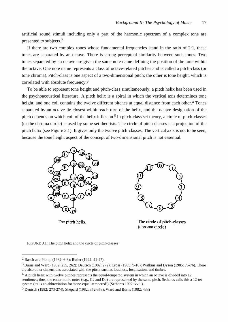
To be able to represent tone height and pitch-class simultaneously, a pitch helix has been used in the psychoacoustical literature. A pitch helix is a spiral in which the vertical axis determines tone height, and one coil contains the twelve different pitches at equal distance from each other.4 Tones separated by an octave lie closest within each turn of the helix, and the octave designation of the pitch depends on which coil of the helix it lies on.5 In pitch-class set theory, a circle of pitch-classes (or the chroma circle) is used by some set theorists. The circle of pitch-classes is a projection of the pitch helix (see Figure 3.1). It gives only the twelve pitch-classes. The vertical axis is not to be seen, because the tone height aspect of the concept of two-dimensional pitch is not essential.
FIGURE 3.1: The pitch helix and the circle of pitch-classes
2 Rasch and Plomp (1982: 6-8); Butler (1992: 41-47). 3 Burns and Ward (1982: 255, 262); Deutsch (1982: 272); Cross (1985: 9-10); Watkins and Dyson (1985: 75-76). There are also other dimensions associated with the pitch, such as loudness, localisation, and timbre. 4 A pitch helix with twelve pitches represents the equal-tempered system in which an octave is divided into 12 semitones; thus, the enharmonic notes (e.g., C# and Db) are represented by the same pitch. Sethares calls this a 12-tet system (tet is an abbreviation for ‘tone-equal-tempered’) (Sethares 1997: xviii). 5 Deutsch (1982: 273-274); Shepard (1982: 352-353); Ward and Burns (1982: 433)
18 Chapter 3
Some experimental observations of perceptual similarity between pitches belonging to one pitch-class have been reported. Deutsch (1982: 272) cited studies by Baird (1917) and Bachem (1954) and stated that when subjects possessing absolute pitch were asked to name notes, they sometimes placed notes in wrong octaves even though they named the notes correctly. In her own study Deutsch also noted that, in a listening test of memory for pitch, the subjects generalised pitches that were displaced by an octave (Deutsch [1973]; cited in Deutsch [1982: 299]).
According to Marvin and Laprade (1987: 225), the tendency to group pitches belonging to one pitch-class is associated with listeners familiar with Western tonal music. According to Hantz (1984: 257), it is unknown whether the idea of octave-related pitches in Western tonal music results from the functional equivalence of octave-related pitches, or whether it is due to the physical properties of the pitch. However, octave generalisation also occurs in other advanced music cultures.6 According to Burns and Ward (1982: 264), octave generalisation is probably a learned concept that has its origins in the octave’s unique position in the range of sensory consonance of complex-tone intervals. Bharucha (1991: 87) states that since harmonic spectra are found universally, the perceptual similarity between octave-related tones might result from the presence of octave harmonics in natural periodic signals. Hence, in his opinion, octave equivalence would presuppose an auditory mechanism that registers spectral similarity.
3.1.2 Interval and interval-class
An interval between two complex tones is the distance between the fundamental frequencies of the tones. Two complex-tone intervals (without any musical context) are perceived as being of the same size when the fundamental frequencies of the complex tones stand in the same ratio. However, owing to their influence on the perception of tone height, the higher harmonics also have some influence on the perception of an interval.
Two pitch-classes (x and y) have two intervals between them (x-y and y-x), and these intervals are complementary mod 12.7 An interval-class is represented by the smaller of the complementary intervals (Forte [1973: 14]).8 An interval-class between two pitch-classes abstractly includes all intervals between every possible pair of pitches that can be derived from the two pitch-classes (for example, an interval and its inversion, or an interval and its compound intervals). Deutsch quoted studies by Plomp and Wagenaar and Mimpen (1973) and Deutsch and Roll (1974) and stated that some evidence for the perceptual similarity of inverted intervals has been obtained with both simultaneous and successive tones (Deutsch [1982: 272, 273, 278-282]).
6 Deutsch (1982: 272); Burns and Ward (1982: 257-258, 262). 7 For mod 12 arithmetic, see Definitions I. 8 The intervals between pitch-classes 1 and 5 are 5-1 = 4, and 1-5 (mod 12) = 1-5+12 = 8. Intervals 4 and 8 are complementary, and the interval-class representing them is 4.
Background II: The Psychology of Music 19
3.1.3 Pitch-class set and set-class
A pitch-class set is a collection of pitch-classes without duplications, and a set-class is a collection of pitch-class sets mutually related by a transformation or by a group of transformations. The most widely used system to classify pitch-class sets into set-classes is transpositional-inversional classification (Tn/I) in which the transformations are transposition and/or inversion.9 This means that those pitch-class sets that can be transformed into each other either by transposition, inversion, or both are members of one set-class. Deutsch (1982: 285-286) considers this classification system problematic:
A fundamental problem with this body of theory concerns the basic equivalence assumption on which it rests. The issue of interval class is a thorny one, and the assumptions of equivalence under [...] inversion are also debatable.
Cross (1985: 12) also points out that the form of equivalence being based on transposition and inversion does raise problems. In his opinion, for example, the equivalence between major and minor triads may exist structurally in music, but it does not seem to make complete perceptual sense.
Many studies have been made to examine whether there is perceptual equivalence between a melodic pitch sequence and one of its transformations (transposition, inversion, retrogression, retrograde inversion, or octave displacements of pitches). Deutsch (1982: 285) cites Garner (1973) who noted that some structures were perceived readily, others with difficulty, and yet others not at all. According to Marvin and Laprade (1987: 225-226), listeners retain brief non-tonal melodies solely in terms of their contours. Krumhansl, Sandell, and Sergeant (1987: 51-52) refer to some studies and state as a result that listeners may perceive the relation between a pitch sequence and its mirror forms when the sequences are short and presented in a musically neutral way.
In their own study Krumhansl et al (1987) used eight different 12-tone sequences (the prime form, inversion, retrograde, and retrograde inversion of two rows). In the first experiment the 12-tone sequences were played to the subjects in a musically neutral way. In the second experiment real excerpts from music were used. In these excerpts the composers had used a wide variety of rhythms and registral placements of the pitches (resulting in a variety of contours and interval successions). The researchers noted that the subjects were able to learn to recognise the prime forms of the two rows. They also noted that the subjects were able to classify the other forms of the rows with the corresponding prime forms in both experiments. However, the proportion of correct classifications was higher when the musically neutral tone sequences were used.
9 For set-classification systems, see, for example, Morris (1982) and Castrén (1989: 34-36).
20 Chapter 3
3.2 CONNECTION BETWEEN PITCH-CLASS SET-THEORETICAL ABSTRACT CONCEPTS AND AURAL ESTIMATIONS: THREE STUDIES Only a few studies have been made of the connection between pitch-class set-theoretical concepts and aural estimations of musical realisations representing these concepts. This section discusses three such studies. The two by Gibson (1988, 1993) examine the effect of pitch-class content on perceptual equivalence of chords. The study by Millar (1984) examines perceptual equivalence of different pitch sets derived from the same set-class.10 3.2.1 The effect of pitch-class content on perceptual equivalence of chords
The effect of octave-related pitches on perceptual similarity of nontraditional chords has been studied by Gibson (1988, 1993). In both experiments the subjects heard chords in pairs. The test items of the studies consisted of two chord pairs. The first chord in both pairs was the same, and the second chord was different. Hence, the test items had always pair (X,Y) followed by pair (X,Z). The subjects were to choose in which chord pair the chords sounded more alike (1988) or more different (1993).
In the 1988 study, the number of pitches in the chords varied from three to nine. In one pair of each item, the two chords contained the same pitch-classes arranged so that the corresponding pitch-classes were never realised in the same octave. In the other pair of the item, the number of identical pitch-classes in the chords varied from two to seven, but again the octave placements of the pitches derived from the corresponding pitch-classes were not the same in the two chords. The subjects tended to rate chords with identical pitch-class contents as more similar to each other than chords with partially non-identical pitch-class contents. This was the case particularly when the chords contained six, seven, or eight pitches. Gibson assumed that perception of similarity in these cases might have been involved with octave-related pitch content. Nine-note chords might, according to him, have been too complex for the perception of octave-related pitches to be meaningful. Gibson also stated that, in chords with only a few pitches, the subjects’ attention might have been caught to the individual voices.
In the 1993 study, Gibson used hexachords. In one pair of each item, the two chords had no pitches or pitch-classes in common. In the other pair of the item, the two chords had from 1 to 4 common pitch-classes, which were represented by pitches either in the same octave (shared pitch content) or in different octaves (shared pitch-class content). Gibson found that non-musicians especially rated the chords with three or four shared pitches as more similar to each other than the chords with no shared pitches. But the shared pitch-class content did not seem to be in connection
10 Samplaski has also studied this as a part of his dissertation (2000). Samplaski’s work is referred to in Section 4.6.
Background II: The Psychology of Music 21
with the subjects’ similarity ratings. Hence, the 1993 study did not support the assumptions raised from the findings of the 1988 study.
As a result of these studies, Gibson states that similarity associated with octave-related pitches might be meaningful in itself, but is not an effective predictor of aural relatedness of chords. Yet he calls for additional research. 3.2.2 Perceptual equivalence of short melodies derived from the same set-class
The recognition of set equivalence in three-note melodies was studied by Millar (1984). The melodic fragments that were used in the study had not, in Millar’s words, ‘obvious connotations of tertian harmony’; hence, for example, the major, minor, diminished, and augmented triads were eliminated. Also the three-note chromatic melody was eliminated because of its familiarity as a subset of the chromatic scale. Altogether Millar made melodies from five triad classes (Tn/I-classification) (1984: 51-52).
Each test item consisted of a standard stimulus and three comparison stimuli. One of the comparison stimuli was equivalent to the standard stimulus under one of five specified transformations. The transformations were ordered transposition (preserving contour), ordered inversion (inverting contour), reordered transposition, reordered inversion, and ordered transposition with octave displacement of one pitch. Of these transformations the first two and the last one preserved the original interval-class succession of the standard stimulus, but only the first one preserved the original interval succession. All these transformations preserved the set-class identity of the standard stimulus.
The other two comparison stimuli were derived from set-classes other than that from which the standard stimulus was derived. These comparison stimuli were designed so that they would give further information about the factors guiding the subjects’ responses. Three modifications of the standard stimulus were used in the test. The first of them held two of the standard’s pitches invariant, allowing the third one to alter. The second one had the same contour as the standard stimulus, but the exact interval succession was not similar. The third modification had the same interval-class succession as the standard stimulus, but the contour was different.
The subjects’ task was to determine which of the comparison stimuli was equivalent to the standard. Millar hypothesised that order-preserving transformations of the standard would be easier to recognise than those involving reordering. Additionally, Millar wanted to examine whether transpositionally equivalent relationships would be easier to recognise than inversionally equivalent ones. Millar assumed that the subjects would be able to perceive some relatedness between two melodies that are equivalent under one of the five mentioned transformations, even though they would not necessarily be able to identify the exact relationship involved.
Millar found that ordered transposition of the standard was indeed the most recognisable of the transformations, and that transpositional equivalence was more recognisable than inversional.
22 Chapter 3
Additionally, it was found that it was difficult for the subjects to recognise association between the melodies if the pitches had been reordered. Both contour and interval succession of the pitches were found to be stronger factors of association between two melodies than was pitch invariance. Two melodies with similar contours were rated as similar more often than two melodies with non-similar contours. Millar concluded that different pairs of melodies in which both melodies were derived from the same set-class possessed varying amounts of aural equivalence, even though the set-classes were small and the melodies limited in character.
Millar used triad classes and three-note melodies. The three individual pitches of the melodies were easy to remember. The subjects were given short lesson of basics of pitch-class set theory before the test; thus the recognition of individual pitches was important. It is, however, obvious that the subjects were not able to use the rules of equivalence taught to them during the tutorial. It is easy to believe this, since Friedmann (1990) used months to teach similar knowledge to his pupils. The result indicating that contour seemed to dominate agreed with the statement of Marvin and Laprade (Section 3.1.3).
CHAPTER FOUR EARLIER STUDIES ON THE CONNECTION BETWEEN THEORETICAL RESEMBLANCE AND PERCEIVED CLOSENESS
Only a few empirical studies have been made on the connection between theoretical resemblance of set-classes and perceived closeness of pitch sets representing the set-classes. Both similarity measures and other types of theoretical resemblance models have been tested in these studies. Six studies are discussed in detail in the following sections, and comments on each study are made. The last section of this chapter makes some general observations about the studies.
The musical realisations representing the set-classes differ from one study to another. In the pioneering study by Bruner (1984) the set-classes were represented both by chords and by pitch successions. The studies by Gibson (1986) and Samplaski (2000) involved chords, and the studies by Stammers (1994) and Lane (1997) involved pitch successions. The study by Williamson and Mavromatis (1997, 1999), which involves chords, is still in progress.
4.1 BRUNER
Bruner (1984) was interested in examining whether an interval-class vector based similarity measure, SIM by Morris (1979/80), would predict how listeners relate pitch sets. In a series of tests Bruner compared values produced by SIM with subjects’ similarity ratings.1 In her tests Bruner used trichords and tetrachords, because:
... the small number of pitches involved would aid the clarity of presentation and allow the listeners to comprehend the intervals quickly. (1984: 28)
In the first test, a number of triad and tetrad classes were represented by both chords and melodic-type pitch sequences. Bruner did not find any clearcut relationship between theoretical resemblance and perceived closeness. 1 For Morris’s SIM see Section 7.4.1 of the present study.

24 Chapter 4
Bruner’s study was also designed to investigate and identify factors that might have guided the subjects’ closeness estimations. Bruner found a number of factors. When the set-classes were represented by chords, the most important factor seemed to be the extent to which the members of a pair could be related to traditional harmonic progression. When the set classes were represented by melodies, the factors that affected the subjects’ ratings were the size and location of the most salient intervals. Bruner wrote:
We can say that these associations may be attributed to the compositional arrangement of the sets, rather than to their inherent structure. (1984: 29)
The next three factors also had a positive correlation with similarity ratings, regardless of the realisation of the sets: first, the number of common pitches in pairs; second, the number of semitones in the pitch sets; and third, the tonal associations of the pitch sets. Bruner stated that the total interval content (and, hence, the SIM-measured similarity) was to be viewed as only one factor among an as yet undetermined number of others that had effects on closeness estimations.
Because the closeness estimations seemed to have such a multidimensional structure, Bruner made a second test. It aimed at isolating and describing the underlying factors that might have had an effect on aurally estimated closeness. In this second test the stimuli were pairs of chords with three pitches. Trichords were chosen because the small number of triad classes did permit pairwise comparison of each set-class with every other set-class.2 The chord pairs were played to the subjects who rated closeness between two chords. Bruner applied multidimensional scaling and hierarchical clustering for analyzing her data.
Bruner compared the two-dimensional solutions analyzed from the subjects’ ratings and the similarity values measured by SIM. She found little correlation between these solutions. Hence, she analyzed the subjects’ ratings to determine what musical characteristics might have been represented by the two dimensions. She interpreted the first dimension as a dissonance-to-consonance continuum. According to Bruner, the second dimension seemed to be related to the perception of salient intervals in each chord. Bruner also made a three-dimensional solution of the subjects’ ratings data. The first two dimensions were interpreted by the same characteristics as those of the two-dimensional solution. The third dimension was explained by a salient interval in each chord.
Two groups of chords emerged in the hierarchical clustering analysis. One group contained chords with strong traditional triadic implications. The other group contained chords with semitones and chords with whole tone implications. Both groups were divided into semigroups that seemed to cluster on the basis of one salient characteristic shared by the chords within the group.
Bruner’s conclusion was that, in her experiments, the theoretical resemblance model did not seem to explain the subjects’ estimations of closeness between chords. Instead, the closeness
2 There were 12 triad classes and 66 pairs, because Bruner used Tn/I-classification.
Earlier Studies 25
estimations seemed to be tied to the context in which the chords were presented. The number of common pitches in the chords of a pair, the spacing of chords, and the registral placement of pitches were choices that either diminished or enhanced the degree of perceived closeness. Bruner wrote that the subjects tended to use traditional constructs of consonance and dissonance and traditional harmonic associations even when they rated nontonal chords. According to her, one reason for the results might have been the subjects’ expertise in tonal music. Bruner considered that it could be possible to ‘increase listener sensitivity to similarity relationships among contemporary pitch structures’ by intensive training.
The chords Bruner used in the second test were trichords. It is more than likely that the chords’ associations with tonal chords influenced the closeness estimations. However, the SIM-measured similarity is not based on the same aspects as associations between chords used in tonal music.3 Additionally, SIM produces only three distinct values for the 66 triad-class pairs (values 2, 4, and 6), but most likely the subjects used finer gradation in their ratings.
Another factor that might have been a reason for the low correlation between theoretical resemblance and perceived closeness was the chordal settings used by Bruner. The highest pitch of the two chords in each pair was kept constant, but the two lower pitches could vary. The method in which Bruner composed the chords did not take into account the number of elements in the largest mutually embeddable subset-class of the set-classes from which the chords were derived. This means that the number of common pitches in the chords of each pair was sometimes the highest possible, sometimes smaller.
Yet another factor that might have influenced the poor connection between theoretical and aural similarity was the width of the two chords in one pair. Sometimes it was the same, sometimes it was not. It is likely that the change in the width influenced perception. But the difference in width between two chords cannot be measured by SIM (nor by any other similarity measure), because the width of a chord is bound to chordal setting of the pitches.
4.2 GIBSON
Gibson (1986) was interested in the connection between theoretical resemblance and aurally estimated closeness of nontraditional chords.4 His question was whether the interval content could provide the basis for perception of closeness between two chords unfamiliar to the listener. Gibson studied a number of theoretical resemblance models, namely, Forte’s Rp and Rn- relation (and
3 For example, the subjects’ ratings suggested a rather close connection between chords derived from set-classes 3-9 and 3-11 in Bruner’s test. As far as can be determined from Bruner’s explanation (1984:31), these set-classes were represented by a major triad and a major triad with four-three suspension. However, the SIM-value for the pair of set-classes 3-9 and 3-11 is 4, the middle one of the three values it produces among triad classes. 4 Gibson’s article is based on his doctoral dissertation (1983).
26 Chapter 4
combinations of these, because, according to Forte [1973: 50)], Rp is not especially significant taken alone) and a similarity measure by Lord (1981) called similarity function.5 Additionally, he studied three set-equivalence relations (namely, transposition, inversion, and Z-relation). In his study Gibson used tetrachords derived from 24 tetrad classes (Tn/I -classification). Because Gibson was especially interested in aural estimations of closeness between nontraditional (nontonal) chords, chords with significant associations with tonal music were excluded.
There were four chords in two pairs (X,Y and X,Z) in each test item, and the subjects were asked to choose in which pair the chords sounded more alike. The outer pitches of the four chords in each item were the same, but the two inner pitches changed. The width and the register of all chords in one item were the same, but the overall variation of width and register was not specified by Gibson.6
According to Gibson, the outcome provided by the selected theoretical resemblance models did not associate with the subjects’ similarity ratings. He stated that the role theoretical resemblance might play in perception of harmonic structures remained to be determined. He also noted that subjects who identified themselves as possessing knowledge of the atonal idiom did not respond differently from the subjects without such knowledge.
In Gibson’s study the width and register of the two chords in one pair were the same, but it is unclear how much they varied throughout the test. A curiosity in the composition of the test items was that the number of common pitches in the pairs was kept constant (it was two; as already stated, the outer pitches of chords in one pair were always the same). The advantage of the constant-number-of-common-pitches decision might have been that the change in the number of common pitches could not affect the subjects’ closeness estimations.
But the disadvantage of the decision was that the cardinality of the largest mutually embeddable subset-class of the two set-classes being compared was not taken into account when the test items were composed. As far as can be determined from the report, in Gibson’s data this cardinality was either two or three. Hence, the largest possible number of common pitches between two chords was either two or three. As the number of common pitches utilised by Gibson was always two, some chord pairs had the maximum number of common pitches, some pairs did not.7
5 Some of the combinations of Forte’s relations unite a relation indicating similarity with one indicating dissimilarity (for example R1 combined with absence of Rp; Forte [1973: 50]). The way in which such combinations were scored by Gibson remained unclear. 6 Gibson only stated that the items were ‘within the outer limits of the usual vocal ranges’ (1986: 14). 7 The number of common pitches is also associated with the Rp relation. This relation holds between two set-classes of cardinality n if at least one set-class of cardinality n-1 is abstractly included in both of them. If two pitch-class sets share fewer than n-1 pitch-classes, but are member sets in two set-classes enjoying Rp, Rp between the pitch-class sets is weakly represented (Forte [1993: 47, 50]). Because n-1 in Gibson’s test was three, but the constant number of common pitches was two, the chords could not have the n-1 pitches in common, and hence the Rp relation could only be weakly represented or absent between the chords being compared.
Earlier Studies 27
4.3 STAMMERS
Stammers (1994) was interested in examining how certain pitch-class set-theoretical concepts might be associated with the perception of short melodies. These concepts were the total interval-class contents of set-classes, set-class equivalence, and inclusion relations. One part of her study examined whether the values produced by similarity measure SIM by Morris (1979/80) correlate with subjects’ similarity ratings. Stammers used tetrad classes and four-note melodies derived from these set-classes.
Each of the 40 test items used by Stammers consisted of four melodies in two pairs (X,Y and X,Z). If the SIM-value for the first pair was 2, the SIM-value for the other pair of the item was 8, and vice versa.8 The subjects, both musically trained and non-musicians, were asked to rate in which pair the melodies were more similar to each other. The four melodies of each item were played within an octave, but the register of the whole test reached from Eb2 to D4. The first pitch of the four melodies of each item was the same, and this pitch was the only common pitch in the melodies of one pair. The other three pitches of melody X were played in random order. Melodies Y and Z had similar contours, and their contour was either similar to that of X or dissimilar to it.
Stammers found that the musically trained subjects considered the melodies of the pair related by SIM = 2 more similar to each other than the melodies of the pair related by SIM = 8. This finding was statistically very significant (p < .008).9 But the ratings made by non-musicians did not correlate with the SIM-values. The difference between ratings made by musicians and non-musicians was statistically significant (p < .020).
Stammers also reported that she had tested whether the changes in ‘successive interval content’ of the melodies would affect the subjects’ similarity ratings (1994: 81-82).10 She compared the successive interval contents of the two melodies of each pair and scored the differences. She hypothesised that subjects would perceive the pair ‘with lower difference between successive interval content as the more similar pair’. This hypothesis was rejected. Unfortunately, Stammers did not show the test melodies, nor did she give a detailed description of the scoring. Hence, the way in which the scoring was done remains unclear for the reader and the result questionable.
According to Stammers (1994: 83-84), in this particular test the results demonstrated that the musically trained subjects’ similarity ratings were based on the total interval contents of the melodic fragments. She added that the experimental conditions were such that the subjects could not use any other means to relate the melodies. It is, however, possible that the ratings were based on other factors, like the ranges of the melodic fragments (that is, the interval between the lowest and the
8 The lowest and highest values SIM can produce when tetrad classes are compared are 0 (maximal similarity) and 10 (maximal dissimilarity); SIM can produce 6 distinct values (Castrén [1994a: 55]). 9 For explanation of significance and p-values, see Definitions II. 10 With ‘successive interval content’ Stammers obviously means the chain of intervals between successive pitches of the melody.
28 Chapter 4
highest pitch of the melody), their chromaticism or diatonic associations, or the interval between the first two pitches, etc.
The number of common pitches was kept constant throughout the test. This decision had the same advantage and disadvantage as was mentioned in the previous section concerning Gibson’s study.
According to the chosen similarity measure, only cases deriving value 2 and cases deriving value 8 were in Stammers’s test. The subjects were asked in which of the two pairs the melodies were more similar to each other. No finer gradation of closeness, resemblance, or similarity was asked from the subjects, nor were such pairs that would derive SIM-values other than 2 or 8 used in the test. Stammers admitted that the subjects might not have been able to identify the closeness between the melodies if the difference in the similarity values would have been smaller. A test like this could not convince the reader of the connection between measured and aurally estimated similarity, because the results of the test confirmed the existence of such connection in some rather extreme cases only.
4.4 LANE
Lane (1997) used different techniques of multidimensional scaling (repeated, weighted, and classical multidimensional scaling) to reveal and identify factors influencing subjects’ estimations of closeness between pitch successions. He was also interested in associations between theoretical resemblance and perceived closeness. Lane tested seven similarity measures. These were SIM and ASIM by Morris (1979/80), MEMB by Rahn (1979/80), REL by Lewin (1979/80), s.i. by Teitelbaum (1965), IcVSIM by Isaacson (1992), and AMEMB, which was Isaacson’s extension of Rahn’s MEMB.11 Lane used 321 pairs of pitch successions derived from 21 set-classes of cardinalities reaching from 3 to 9. These pairs were rated by subjects. However, similarity values were derived only for 21 set-class pairs, and in all these pairs one of the set-classes was 3-1 (these values were taken from Isaacson [1992]). These 21 pairs were the sample when the connection between theoretical resemblance and perceived closeness was examined.
The stimuli of the empirical test were successions of ascending pitches. The length of the stimuli varied, because the duration of each pitch was the same, but the number of pitches varied in accordance with the cardinality of the set-classes from which the pitches were derived.
11 All measures tested by Lane compared interval-class contents of two set-classes. Hence, Lane actually used MEMB2, AMEMB2, and REL2; see Isaacson (1992: 49-65).
Earlier Studies 29
Lane presented 17 variables which, in his opinion, represented prominent attributes of the stimuli used in his test. The connection between these attributes and the dimensions analyzed from subjects’ similarity ratings were examined by multiple regression.
Lane explained the subjects’ similarity ratings with a four-dimensional solution. The first dimension was interpreted as being associated with the number of pitches and intervals of the stimuli (that is, the cardinality of the set-classes from which the pitch successions were derived), the chromaticism of the first pitches, the diminished triad as a subset of the stimuli, and the number of common pitches in two stimuli. Additionally, there was a strong association between the first dimension and values produced by five similarity measures (MEMB2, REL2, s.i., SIM, and ASIM).
The second dimension was interpreted as having tonal associations. The third dimension was interpreted as being associated with the outer interval of each stimulus, the intervals between the successive pitches of the stimuli, symmetry of the stimuli, and the augmented triad as a subset of the stimuli. Additionally, an association was found to exist between the third dimension and values derived from two measures (IcVSIM and AMEMB2). Lane explained the fourth dimension by two attributes: first, the tritone in a nonchromatic context versus the tritone in a chromatic context; and second, the augmented triad.
As a conclusion, Lane (1997: 199) stated that the prominent attributes guiding the subjects’ closeness estimations were the cardinality of the set, intervals between the successive pitches, tonal and atonal associations, and symmetrical structure. He also found a connection between values derived from similarity measures and the subjects’ similarity ratings. This connection was reported as ‘a strong association’ for measures MEMB2, REL2, s.i., SIM, and ASIM; and ‘an association’ for IcVSIM. At the end of his dissertation Lane called for further research to investigate the connection between theoretical resemblance and perceived closeness.
The four-dimensional solution Lane found in his analysis did not reveal any clear structure. Three of the dimensions were interpreted by many attributes. Additionally, it is difficult for the reader to understand the connection between, for example, the attributes by which the first dimension was interpreted (the cardinality of the set, the chromaticism of the first pitches, the diminished triad, the number of common pitches). The finding that the cardinality of the set was important for perception is understandable in itself, because even small differences were easy to recognise from the length of the stimuli.
There was also one problem in using some of the similarity measures for the mentioned set-class pairs: s.i. by Teitelbaum was originally designed only for set-classes of the same cardinality (Teitelbaum [1965: 88]); and even though Morris designed his SIM for both the same and different cardinalities, he presented his ASIM ‘In order to relate similarity indices derived from pairs of sets of any cardinality’ (Morris [1979/80: 446, 449, 450]). Additionally, according to Castrén (1994a: 55, 76), there are serious problems in the scales of values produced by SIM and MEMB2 when set-classes of different cardinalities are compared, and this is the case for s.i. as well. Yet another problem in the test arrangement was that there were measured similarity values for only 21 set-class
30 Chapter 4
pairs out of 321, and in all these 21 pairs one member of the pair was always set-class 3-1. Hence, the association between theoretical resemblance and perceived closeness found by Lane must be accepted with reservations.
4.5 WILLIAMSON AND MAVROMATIS
The question posed by Williamson and Mavromatis (1997, 1999) was how theoretical resemblance relates to perceived closeness. Their basic intention was to define a perceptually-based similarity measure. To do this they applied the techniques of multidimensional scaling (1997), tree-fitting, and clustering (1997, 1999) to subjects’ ratings of similarity between pairs of chords. The scaling techniques were chosen to identify factors that contribute to perceived closeness. Additionally, Williamson and Mavromatis examined the factors and their correspondence to some theoretical resemblance models.
Williamson and Mavromatis chose theoretical resemblance models from two categories: models comparing interval-class contents of set-classes (SIM by Morris [1979/80] and Regions by Ericksson [1986]) and models comparing subset-class contents of two set-classes (REL by Lewin [1979/80] and RECREL by Castrén [1994a]).12 However, their research has thus far focused on comparing the subjects’ ratings with the outcome provided by the two interval-class content-based models. Comparison with subset-class content-based models is still in progress.
In their 1997 study, Williamson and Mavromatis used four-note chords and musically expert subjects. Shepard tones were used to minimise the effects of register and contour (it is likely that with ‘contour’ of chords Williamson and Mavromatis indicate the width of the chords and the intervals between adjacent pitches). As far as can be determined from their report, there were chord pairs with maximum number of common pitches and those with no common pitches at all. Additionally, chords derived from all but one set-class were played on four different transpositional levels.
Williamson and Mavromatis reported a correlation between similarity ratings and theoretical resemblance for the two examined models (Morris’s SIM and Ericksson’s Regions). Additionally, they reported that an increase in the number of common pitches between the chords contributed to an increase of perceived closeness.
Williamson and Mavromatis applied a neural net model to the similarity rating datasets from each subject. Nine subjects’ datasets were excluded from further analysis, because the neural net model could not predict the subjects’ ratings. Individual difference scaling analysis was applied to
12 Three of the models (SIM, REL, and RECREL) are similarity measures.
Earlier Studies 31
the remaining 26 datasets.13 Williamson and Mavromatis described the data of tetrachords by a five-dimensional solution. Three dimensions were interpreted as representing the effect of common pitches and two dimensions as reflecting set-class similarity.14
In their 1999 study Williamson and Mavromatis used six-note Shepard-tone chords. The subjects were both musically experienced subjects and non-musicians. The chords were played on 2, 3, or 4 transpositional levels. These data were represented by a six-dimensional structure. Two dimensions were interpreted as representing the set-classes of the study and four dimensions as representing the effect of common pitches.
The study by Williamson and Mavromatis is still in progress. The reports are not systematic descriptions of their work, and, furthermore, the interpretation of the dimensions seems incomplete. Their conclusions thus remain open.
4.6 SAMPLASKI
Samplaski (2000) examined perceived chordal closeness. He analyzed the subjects’ similarity ratings by multidimensional scaling and hierarchical clustering to examine the factors guiding the ratings. He also compared the subjects’ ratings with four chord-classification systems. These systems were by Hindemith (1937/1942), Forte (1988), Harris (1989), and Quinn (1997).15
Three different experiments were conducted in the study, one after another. Seventy musically experienced subjects participated. The test items were chord pairs, and the subjects were asked to rate similarity between the chords in each pair on a seven-step scale. Each pair was presented in both orders (X,Y) and (Y,X); the chords were not paired with themselves. All tests included so-called regular trials (all pairwise comparisons of the test chords) and a set of randomly selected re-test trials. Trials were presented in random order, separately for each subject.
The subjects heard the tetrachords played in two timbres: a pseudo-clarinet sound and Shepard tones. According to Samplaski (2000: 12), these timbres were used in order to assess how subjects' estimations might change when they could and could not discriminate pitch-height. The timbres were not mixed; clarinet-sound chords were paired only with other clarinet-sound chords, while Shepard-tone chords were paired with other Shepard-tone chords.
13 As far as can be determined from their report, Williamson and Mavromatis used 53 chords. Of these (53*52)/2 = 1378 pairs can be formed. According to the report, 35 pairs were estimated by the subjects; the rest (1343 pairs) were obviously estimated by neural nets. 14 By ‘set-class similarity’ Williamson and Mavromatis actually mean the same chord played on four transpositional levels. 15 None of these chord classification systems is actually a theoretical resemblance model. However, Samplaski’s study is so closely connected to the present one and to the other studies referred to in this chapter that it is discussed here.
32 Chapter 4
In Experiment 1, the test material consisted of 30 chords derived from 11 set-classes (from 1 to 4 chords from each set-class; Samplaski [2000: 100-105]).16 Widths of the chords varied from 6 semitones to 16 semitones. Fourteen chords had closed spacings, with the width varying from 6 to 9 semitones. Sixteen chords had open spacings, with the width varying from 13 to 16 semitones.
In the first section of Experiment 1 (called below Experiment 1A), the 30 chords were played in 870 pairs in the pseudo-clarinet timbre. The width of the chords in one pair could be the same or could vary. The lowest pitch of the chords was always the same (C4). In the second section of Experiment 1 (called below Experiment 1B), 17 of the 30 chords were played in 372 pairs as Shepard tones.
Experiment 2 was, according to Samplaski (2000: 106), aimed at ‘evaluating perception of the basic pcset theory operations Tn/TnI’. This experiment used chords derived from four set-classes (4-16A, 4-16B, 4-Z29A and 4-Z29B). Two chords, one with an open spacing and one with a closed spacing, were derived from each set-class. Each chord was played on three different transpositional levels. This made 24 chords altogether (4*2*3 = 24) and 552 pairs. The chord pairs together with the re-test trials were played in the pseudo-clarinet timbre.
Experiment 3 was, according to Samplaski (2000: 109), aimed at ‘assessing subjects’ perceptions of chord similarity under the experimental condition where the pitch-height between outer voices was fixed’. The test material consisted of all possible tetrachords with the width of 7 semitones, a total of 15 chords (derived from 14 tetrad classes). The 210 chord pairs, derived from these 15 chords together with the re-test trials were played in the pseudo-clarinet timbre.
The data gathered in these experiments were analyzed by multidimensional scaling and an additive tree (cluster) analysis. Each dataset was analyzed separately; various subsets of the data in Experiments 1A and 1B were also extracted for separate analysis.
The results of Experiment 1A (the pseudo-clarinet tone dataset) showed that the most important factor guiding the subjects’ closeness estimations in the test was the width of the chords. The open-spaced chords grouped together, and the closed-spaced chords grouped together. Analysis of each of these groups as well as analysis of further subsets of the data revealed other factors: the exact width of the chords, the relative pitch height of the inner voices (resulting in ‘top-heaviness’ or ‘bottom-heaviness’ of the chords), the even or uneven distribution of pitches, and the interval-class contents of the chords (Samplaski 2000: 131-162).
The analyses of the Shepard-tone dataset (Experiment 1B) revealed two main factors. These two factors were interpreted as ‘evenness of distribution of pitch-classes’ on the pitch-class circle, and the shared pitch-class contents of the two chords. Analyses of subsets of the data also revealed other factors, for example, ‘top-heaviness’ or ‘bottom-heaviness’ of the chords (Samplaski 2000: 166-182). According to Samplaski (2000: 166), it was apparently possible for the subjects to hear ‘top-
16 In this report of Samplaski’s study, the Tn-classification is used, even though Samplaski used Tn/I-classification in his dissertation.
Earlier Studies 33
heaviness’ in Shepard-tone chords, even though they could not discriminate pitch height. He hypothesised that since the subjects had heard the clarinet-timbre chords with C4 as the bass pitch several hundred times, this would have given the pitch-class C a privileged status as a bass pitch-class.
The results of Experiment 2 showed that the transpositionally related chords grouped together, but the chords derived from two inversionally related set-classes did not (2000: 191).
Interpretation of the results of Experiment 3 (the clarinet-timbre chords with the same width) was, according to Samplaski (2000: 192), problematic. It seemed that multiple competing simultaneous factors guided the closeness estimations in these pairs. These factors were the relative pitch-height of the alto and tenor voices, trichordal subsets, distribution of the pitch-classes on the pitch-class circle, and the exact interval between alto and tenor voice.
According to Samplaski (2000: 145, 150, 158, 162, 170, 178, 182, 203, 204), the subjects’ ratings did not match any of the four chord-classification systems in any of these experiments. He (2000: 230) concluded:
The results of this study suggest that multiple factors contribute to the strategies listeners use in judging the similarity of non-tonal sonorities, and that these factors interact or compete in different domains, leading at times to a complex structure.
One reason for the complex structure that was found to guide the subjects’ closeness estimations might have been the enormous number of test trials of Samplaski’s study. The test trials possessed a variety of chordal factors that could be used as guides by the subjects. It was found that one of the most important factors was the width of the chords: the smaller the difference in widths, the smaller the dissimilarity between chords. The problem in the testing procedure was that the width of the chords was also sometimes the same in both chords of a pair. However, the same width in both chords did not indicate similarity between the chords. When estimating the pairs in which the width was the same, the subjects had to use some other criteria for their ratings.17 It is likely that the results would not have been as complex as they are now if the test items belonging to these two categories (different widths and the same width) had been presented separately in two different tests.18 Additionally, it is not clear whether the factor guiding the subjects’ ratings was the width of the chords as such. It is also possible that the subjects were actually listening to the absolute height of the highest pitch (as stated earlier, the lowest pitch of all chords was the same).
17 For this reason Samplaski had to analyze some subsets of the data separately. 18 According to Samplaski (2000:192), the subjects reported that it was difficult to make ratings in Experiment 3 (the clarinet-timbre chords having the same width).
34 Chapter 4
Samplaski did not try to set up a control for the number of common pitches in chord pairs (2000: 217), nor did he try to examine the importance of common pitches for the closeness estimations. Hence, he did not take into account the number of elements in the largest mutually embeddable subset-class of the set-classes from which the chords were derived.
4.7 SOME OBSERVATIONS ON THE EARLIER STUDIES
Of the studies cited above, Isaacson (1997: 237-238) mentions those of Bruner, Gibson, and Stammers. He comments that the context in which the stimuli were presented in these studies seems to have had a strong effect on perception. In his opinion, many of the studies tested aspects of pitch-class set theory that are outdated. By this, he presumably means those theoretical resemblance models that are not designed to describe resemblance between any set-class pair, but can only be used for limited material. Additionally, he writes that most of the studies worked with very restricted material (for example, trichords only). According to Isaacson, the predictions resulting from such studies may not easily be generalised to the full space of pitch-class sets.
Many studies with well-controlled material and in well-controlled conditions will be needed before the ‘full space of pitch-class sets’ can be understood. The author thinks that the problem arising from the use of trichords in the studies cited above was not the fact that the material was restricted. Rather the problem was that many three-note pitch combinations have strong tonal associations. As already stated, theoretical resemblance between set-classes is based on aspects other than, for example, tonal chord functions or learned connections between familiar tertian chords.
Contrary to the opinion of Bruner, the author believes that it is not necessary for subjects to be able to analyze the individual pitches and intervals of the test chords. It should be possible for the subjects to make similarity ratings between chords according to some kind of overall impression of them.
Some common factors guiding estimations of closeness between pitch sets, whether melodies or chords, were reported in the studies cited above. These factors were the number of common pitches in pairs, tonal associations of the pitch sets, and the semitones or chromaticism of the pitch sets. Also the size and location of the most salient intervals was mentioned in more than one study. The importance of the width of the chords (tested only by Samplaski) also seems to make sense on an intuitive level.
In the studies discussed above, the connection between perceived closeness and theoretical resemblance was either poor or was not found at all. One reason for this seems to have been the way in which the chord pairs for the tests were composed. Some variables of chordal setting were not controlled systematically. One of these variables was the width of the two chords of each pair. Another was the number of common pitches in the chords of a pair and the connection between this

Earlier Studies 35
number and the cardinality of the largest mutually embeddable subset-class of the set-classes from which the chords were derived. Additionally, in some cases unsuitable theoretical resemblance models were tested or the models were used in some inappropriate way. The variables of chordal setting will be discussed further in Chapter 10 when the chords and chord pairs will be composed for the present study. The theoretical resemblance models will be selected in Chapter 7.

CHAPTER FIVE ON CONSONANCE AND DISSONANCE
The way in which the concepts ‘consonance’ and ‘dissonance’ have been used in Western polyphonic music has varied from one historical period to another. Tenney (1988) discusses five distinct concepts of consonance. These are ‘melodic’, ‘polyphonic’, ‘contrapuntal’, ‘functional’, and ‘sensory’ consonance or dissonance. According to Tenney, the first four types are strictly bound to the musical context from which they arise (‘musical’ consonance). But the concept ‘sensory consonance’ (also ‘tonal’ consonance) is used in the literature in a perceptual sense, to refer to sound stimuli without any musical context.1 Tonal consonance relates consonance to smoothness and absence of beats, while dissonance is related to roughness and presence of beats caused by interacting partials.
It seems that the degree of estimated consonance has always been an important factor in listening experience. For this reason, aspects of tonal consonance and musical consonance of intervals are discussed in Section 5.1. Section 5.2 explains some theoretical models of tonal consonance for intervals and interval-classes. These models will be needed when the results of the study are analyzed (in Chapters 12 and 13).
5.1 TONAL CONSONANCE AND MUSICAL CONSONANCE OF INTERVALS
The tonal dissonance of an interval consisting of two simultaneous pure tones (sine waves) seems to be due to interference between them. It was found by Plomp and Levelt (1965: 553-555) that the dissonance is well described by critical bandwidth. Critical bandwidth is the region of basilar membrane on which two sine waves cause significant overlapping of the ripples of the hair cells (see, for example, Sethares [1998: 86]). According to Risset and Wessel (1982: 28), critical
1 Because the term ‘sensory consonance’ refers to the sense receptors and nerves of the auditory system, the term ‘tonal consonance’ will be used in the present study. In this context, the word ‘tonal’ should not be confused with tonality.
On Consonance and Dissonance 37
bandwidth around a certain frequency is the range within which this frequency interacts with others. Critical bandwidth also explains the loudness of a sound: When pure tones are added to stimuli within the critical bandwidth (keeping the total energy of the sound constant), they do not add the loudness of the sound, because they mask each other (see, for example, Dowling and Harwood [1986: 49-50]). Experience of dissonance occurs if the frequency separation between the two pure tones is less than one critical bandwidth. According to Plomp and Levelt (1965: 555), the most dissonant pure-tone intervals are at about one-quarter of the critical bandwidth.
The tonal consonance of an interval between two complex tones has been explained by frequency ratio between the pitches, by relationships of harmonics of the complex tones, by beats between harmonics, by difference tones, or by fusion (see Plomp and Levelt [1965: 549-550]). Plomp and Levelt (1965: 555) explain the consonance of two complex tones both by the distance between the fundamentals and the distance between the harmonics. According to them, the consonance can be described as a function of the interval width with the critical bandwidth as the unit. Additionally, they assume that the total consonance is equal to the sum of the consonances of each pair of partials. Sethares (1998: 75) suggests that the tonal consonance of complex-tone intervals depends both on the interval between the tones and the spectrum of the tones. If the tones have nonharmonic spectra, the partials might ‘clash raucously when played in a simple 2/1 octave’, resulting in the experience of dissonance.
Contrary to tonal consonance, ‘musical consonance’ is related to the rules of music theory, and can, to a certain extent, operate independently from tonal consonance. The degree of estimated musical consonance of tone combinations can be strongly affected by the listener’s experiences, expectations, and what the listener has learned. If the listener understands the context in which two simultaneous tones sound together, he or she can learn to hear the combination as musically consonant or dissonant. For example, combinations that require resolution can be heard as musically dissonant, regardless of their tonal consonance (see Karma [1986: 20]). However, it seems that in general musical consonance is based on tonal consonance of complex tones.
Terhardt’s (1982: 362, 1984: 276) definition of musical consonance is based on two main components. These components are ‘sensory consonance’ and ‘harmony’. According to Terhardt, ‘sensory consonance’ represents the universal aspect of pleasantness or non-annoyance, and it is a universal aspect not only of music, but of any sound. ‘Harmony’, in turn, represents music-specific principles, that is, the essential functional features of Western tonal music. Whether a particular interval is judged as consonant or dissonant depends, according to Lundin (1967: 90-100), on both ‘natural law theories’ and ‘cultural theories’. The physical properties of a sound, for example, overtones, beats, roughness, and frequency ratio between two tones, are parts of ‘natural law theories’ (tonal consonance), whereas responses of consonance or dissonance are influenced by our cultural background (musical consonance). Leman (1991: 100) states that the ‘sensory aspect’ of tonal semantics (not only consonance or dissonance) is related to the acoustical properties of the stimuli and the sensory properties of the ear. The ‘cognitive aspect’, as Leman calls the other
38 Chapter 5
component, explains what is added to the stimuli by the cultural character of music and by the learning processes of the listener.
Plomp and Levelt (1965: 550-551) point out that the consonance perception of a Western listener is influenced by the development of Western tonal music and musical training. They state that the original concept of consonance has been divided into two components, of which one is characteristic of musicians and the other, of untrained listeners: musicians distinguish between consonance and pleasantness, but untrained listeners equate consonance with pleasantness. Additionally, musicians maintain the learned rank order of intervals in terms of consonance. It is possible that the tonal consonance of musical events is more important for musically inexperienced listeners’ ratings, while musical consonance is more important for musically experienced listeners.
5.2 MODELS OF TONAL CONSONANCE FOR INTERVALS AND INTERVAL-CLASSES
Three models of tonal consonance for complex tone intervals or interval-classes will be utilised in this study (see Sections 9.3 and 10.2).2 The models for intervals are from Malmberg (1918) and Kameoka and Kuriyagawa (1969), and the model for interval-classes is from Huron (1994). All these models give indexes for intervals or interval-classes. These indexes are numerical values indicating the degree of consonance of each interval or interval-class.
The model by Malmberg (1918) is based on musically experienced subjects’ ratings in an empirical test (see Krumhansl [1990: 55-56]). In Malmberg’s test, only the interval size of the items was manipulated; the intervals were played by a piano or by tuning forks. According to the Malmberg model, the most consonant intervals are the perfect fifth, major sixth, and perfect fourth, respectively.3 The most dissonant interval is the minor second, and the next are the major second and major seventh.
The model by Kameoka and Kuriyagawa (1969) is based on Plomp and Levelt’s (1965) ideas of dissonance explained by the critical bandwidth. Kameoka and Kuriyagawa calculated the total consonance of paired complex tones with two to eight harmonics. They also compared their theoretical calculations with musically inexperienced subjects’ consonance ratings. They noted that the subjects’ ratings agreed well with the theoretical calculations. According to this model, the most consonant intervals are the perfect fifth, perfect fourth, and major sixth, respectively, and the most dissonant intervals are the minor second, major second, and major seventh, respectively.4
2 The term ‘model of consonance’ will be used throughout this study, even though the model by Kameoka and Kuriyagawa (1969) is designed so that the highest values indicate the highest degree of dissonance (hence, it is actually a model of dissonance). 3 The Malmberg indexes for intervals will be given in Section 10.2. See also Plomp and Levelt (1965: 551). 4 The Kameoka and Kuriyagawa indexes for intervals will be given in Section 10.2
On Consonance and Dissonance 39
The Kameoka and Kuriyagawa indexes for complex-tone intervals with six harmonics were chosen to be used in the present study. The values were estimated by Krumhansl (1990: 56) from the graph given in Kameoka and Kuriyagawa (1969: 1465).
Huron (1994) studied tonal consonance of pitch-class combinations. Huron introduced a model of consonance for interval-classes called ‘Interval class index of tonal consonance’. Huron stated that interval size alone does not entirely account for the perceived degree of consonance of two simultaneous complex tones; spectral content, sound pressure level, and pitch register are important as well (1994: 292-293). Hence, according to Huron, his index could be regarded as a rough approximation of the degree of consonance of equally tempered interval-classes. Huron’s model is based on three models of tonal consonance for intervals, namely, those of Malmberg (1918), Kameoka and Kuriyagawa (1969), and Hutchinson and Knopoff (1979). Huron’s model is an averaged and normalised modification of the three mentioned models. According to Huron’s model, the most consonant interval-class is 5, and the most dissonant interval-class is 1.5
5 The Huron indexes for interval-classes will be given in Section 9.3.
CHAPTER SIX ON RELIABILITY AND VALIDITY OF TESTING
Two tests (the chord-pair test and the single-chord test; see Section 1.3) were devised in the present study to collect the empirical data. The idea was that some tendencies concerning perception can be revealed by statistical analyses of the ratings made by subjects, even though the subjects themselves would not be conscious of the factors influencing their ratings. The two questions that must be discussed are whether the subjects could rate the chords reliably (the question of reliability; Section 6.1) and whether the tests measured what they were meant to measure (the question of validity; Section 6.2).
6.1 ON RELIABILITY OF TESTING
The term ‘reliability’ is generally used to indicate the consistency of a test. The test is said to be reliable if it yields the same results when administered two or more times under similar conditions. The reliability of a test can be increased by examining the subjects’ responses to individual test items and by excluding those items that are not answered consistently vis-à-vis the responses to the other items.
Reliability coefficients can be calculated for tests. These measures are usually based on correlations between different test items. The idea behind many reliability coefficients is the assumption that all test items measure a common entity. This is why the items should be positively correlated with each other. The most commonly used reliability coefficient is Cronbach’s Alpha.
However, this kind of reliability control would be impossible in the chord-pair test as well as in the single-chord test. As stated in the Introduction, the closeness estimations are usually made by determining identity across many dimensions simultaneously. The relative importance of different
On Reliability and Validity of Testing 41
dimensions varies from case to case and from one subject to another. This would probably lower the correlations between test items, and, hence, lower the reliability coefficient.
In the single-chord test, the ratings on a single semantic scale are not likely to be multidimensional. Yet it is not possible to examine the consistency of the ratings on, for example, the scale ‘barren - lush’, because the chords do not possess any measurable property that could be called ‘lushness’. Hence, it is not possible to compare the subjects’ ratings with the ‘correct amount of lushness’. This is the case for any scale. The subjects’ ratings in both tests are based on their opinions. It is likely that different subjects use the rating scales in different ways. The subjects’ reasons for certain ratings are undefined and unknown; thus every reason for the ratings must be considered equally acceptable. According to Cronbach (1990: 192), in test theory the term ‘error’ refers to unwanted variation. In the present tests, the variation in responses for each stimulus is due both to differing opinions and to error.
Because there are no correct answers with which the subjects’ ratings could be compared, the question of reliability must be approached in some other way. It is possible to calculate the arithmetic mean of all subjects’ ratings for each item. The arithmetic mean can be said to show some tendency of what the closeness between two chords could be, or whether one chord could be called ‘lush’ or ‘barren’.
It is also possible to calculate correlations between each individual subject’s ratings and the arithmetic mean of ratings of all other subjects. High correlations would indicate that the subjects rated the chords consistently with other subjects, and most likely, consistently with themselves as well. Low correlation would indicate inconsistency of the subject compared with other subjects. But in a study such as this, low correlations between some subjects’ ratings and the arithmetic mean of all other subjects’ ratings will not necessarily indicate inconsistent ratings from these particular subjects. It is possible that such subjects would have made their ratings in a consistent way, but that the criteria for the ratings by these subjects would have been different from the criteria of the other subjects. Hence, these subjects would have used the scales in different way from the others.
The most accurate method for controlling the consistency of the subjects with themselves would be to test the same subjects again after a lapse of time. However, this method too would create problems. It would be very difficult to motivate the subjects to take the same test again. Furthermore, the subjects could not answer anonymously if the ratings made by a particular subject in the first run were to be compared with the same subject’s ratings in the second run.
Therefore, instead of a test-retest pattern, some control-chord pairs were used in the chord-pair test to examine the subjects’ consistency with themselves. It seemed likely from the very beginning that the subjects with low consistency in the control-chord test and with low correlations with the other subjects’ ratings would be unreliable.
It seems that the answers concerning questions of test reliability must also be found in the test results. The testing can be considered reliable if the underlying solutions revealed in the analyses are clear and interpretable, and if a reasonable amount of variance is explained by the solutions.
42 Chapter 6
Additionally, the testing can be considered reliable if there are connections between results derived from the single-chord test and the chord-pair test analyzed by the different methods. In other words, it seems unlikely that clear and reasonably interpretable results could be revealed with data collected in an unreliable test. And it seems highly unlikely that results derived from two datasets collected in two totally different testing procedures could be reasonably explained by the same attributes if both tests were unreliable.
6.2 ON VALIDITY OF TESTING
A test is said to be valid if it measures what it is intended to measure. The question of whether the two tests of the present study measure what they are intended to measure is not easy to answer. As stated in the previous section, there are no criteria by which one could unambiguously call two chords ‘close’ or ‘distant’ to each other, or call any single chord ‘lush’, ‘barren’, ‘clear’, and so on. One criterion with which the results of the chord-pair test must be compared are the results derived from corresponding tests.
Cronbach (1990: 178-179) states that the interpretation of test results can be supported by putting many pieces of evidence together. If an experiment were made to test some abstract concept, the results might validate the experiment and the concept simultaneously. One aim of the chord-pair test is to test pitch-class set-theoretical similarity measures. If high and statistically significant correlations are found between the measured similarity values and the subjects’ similarity ratings, the measures and the test can be said to validate each other.
According to Cronbach (1990: 145), validation is the inquiry into the soundness of the interpretations made on the basis of scores from a test. It is also possible to say that validity is the degree to which testing procedures and interpretations help the researchers to examine what they want to examine. In the two tests of this study, the question of validity can be partly answered by the same arguments as were made in the question of reliability. Hence, the interpretability of structures and the amount of explained variance are important from the validity perspective as well. It will also be important to compare results derived from the two datasets analyzed by the three methods.
Two factors were controlled to make the present tests as reliable and valid as possible. First, the stimuli were made so that there was as little irrelevant information as possible. Second, the chordal setting of the test chords was controlled as strictly as possible (for chordal setting, see Chapter 10). Hence, the test examined only those characteristics that were relevant for the required information. The number of stimuli was large enough to give answers to the questions that interested the researcher. However, the tests were rather short, and, thus, it seemed likely that the subjects were

On Reliability and Validity of Testing 43
able to concentrate on their task. Additionally, the test form was easy to fill out, and the scoring was unambiguous (for the testing procedure, see Chapter 11).


45
PART II THEORETICAL RESEMBLANCE BETWEEN SET-CLASSES
The second part of the study deals with pitch-class set-theoretical resemblance models. As stated in the Introduction, this study discusses and analyzes certain types of these models, namely, similarity measures. Ten such measures are analyzed in Chapter 7. The conclusions of these analyses are drawn in Chapter 8 when the similarity values produced by the measures are compared.

CHAPTER SEVEN SIMILARITY MEASURES
The first similarity measure (the similarity index, ‘s.i’.) was presented by Richard Teitelbaum as early as 1965, soon after Forte’s first studies concerning pitch-class set-theory.1 The latest measures (up to the present) are the different saturation-based measures presented in Buchler (1998) and the ANGLE presented by Scott and Isaacson (1998).
This chapter analyzes a number of similarity measures. Before these analyses can be done, the connection between set-classification and measured set-class similarity is discussed in Section 7.1. This connection is important, because the chosen set-classification determines the universe of objects that can be compared. Section 7.2 defines the criteria according to which the measures will be selected in this study, since only some of the similarity measures will be examined. Section 7.3 describes the statistical procedures by which the set-class similarity datasets will be analyzed. The analyses are in Sections 7.4 (measures comparing interval-class vectors) and 7.5 (measures comparing subset-class vectors).
7.1 MEASURED SIMILARITY AND SET-CLASSIFICATION
Different types of set-classification systems have been introduced in pitch-class set-theoretical literature.2 Of these Tn/I (transpositional and/or inversional) and Tn (transpositional) classification are the most common.3 Neither of these classifications is inherently better than the other, but Tn/I is the more widely used.
Even though nearly all similarity measures have originally been discussed under Tn/I-classification, Tn-classification was chosen to be utilised throughout the study. This was done 1 Forte’s studies ‘Context and continuity in atonal work. A set-theoretic approach’ (Perspectives of New Music) and ‘A theory of set-complexes for music’ (Journal of Music Theory) were published in 1963 and 1964 respectively. 2 For a discussion of set-classifications, see Morris (1982) and (1987: 78-84); Castrén (1989: 34-36) and (1994a: 31-32). 3 For Tn-classification and Tn/I-classification, see Definitions I.
48 Chapter 7
because the inversionally related set-classes were considered to be individual entities. Hence, all similarity measures will be compiled under Tn-classification regardless of whether they have been designed under Tn or Tn/I-classification. The conditions in which the similarity values will be calculated are thus equal for all similarity measures. Below, the type of set-classification will be mentioned only if it is not Tn.
7.2 CRITERIA FOR SELECTING SIMILARITY MEASURES
Isaacson (1992), Hermann (1994), Castrén (1994a), and Buchler (1998) categorise and analyze a large number of similarity measures and other theoretical resemblance models. Additionally, Isaacson (1990: 2), Castrén (1994a: 17-31), and Buchler (1998: 19-30) discuss conditions a similarity measure should meet before it can be said to serve its purpose well. This study refers to the criteria defined by Castrén.
The similarity measures that will be selected must fulfil three criteria. In Castrén (1994a: 18) these three criteria are called C1 (measures should allow comparisons between set-classes of different cardinalities); C2 (measures should provide a distinct value for every pair of set-classes); and C3.1 (measures should provide a comprehensible scale of values so that all values are commensurable). The motive for choosing these particular criteria is solely practical, and it is connected with the statistical analyses that will be made. The connection between the criteria and the analyses is discussed below.
In this chapter, statistical analyses of the shares of values produced by different similarity measures will be made. Additionally, correlations will be calculated between measured and aurally estimated similarities in Chapter 12. Hence, the outcome provided by the measures need to be quantitative (numeric similarity values on some known scale of values; criterion C2).4 Further, similarity values between set-classes of nearly all cardinalities will be used as the data for the analyses (however, the connection between theoretical and aurally estimated similarity will be examined by using only pentad classes and pentachords). For this reason, the similarity measures must be designed for pairs of set-classes of both the same and different cardinalities (criterion C1), and they need to produce values that are commensurable regardless of the cardinalities of the set-classes being compared (criterion C3.1).
To make the comparison of similarity values produced by different similarity measures clearer, the ranges of values produced by each measure will be modified so that all values are on the same scale. This does not change the ratios between values. Values 0 and 100 will be used as extreme values, with value 0 indicating the highest degree of similarity.5 Thus, what will actually be 4 This was actually presupposed already in the definition of a similarity measure (see Section 1.2). 5 In criterion C3.2 Castrén calls for extreme values that can be meaningfully associated with minimum and maximum similarity (1994a: 20).

Similarity Measures 49
measured is dissimilarity (or distance) between set-classes. Additionally, all values will be systematically calculated as integers.6 Below, each measure is first discussed in its original form. Whenever the range of values of a given measure is modified on the scale from 0 to 100, the symbol ‘prime’ will be added to its name (for example, ASIM-prime).
7.3 STATISTICAL ANALYSIS OF SHARES OF VALUES PRODUCED BY SIMILARITY MEASURES
As already stated, the shares of similarity values produced by the measures will be examined statistically in the following sections. These analyses will be referred to in Chapter 8, when the different measures and the values produced by them are compared. Before the analyses will be done, the statistics as well as the datasets to be analyzed will be briefly discussed.
Two set-class similarity datasets, value group #3-#9/#3-#9 with 56,280 values and value group #5/#5 with 2,145 values, will be generated to be analyzed.7 The first value group was chosen because it contains approximately 91% of all possible set-class pairs.8 The second was chosen because the empirical tests were made with pentachords. The similarity values for the analyses were calculated with computer programs by Castrén (1994b).
The statistical analyses consist of measures of central tendency (the arithmetic mean, the median, the mode); measures of variability (the range, the first and the 99th percentile, the lower and the upper quartile, the standard deviation); and the skewness value.9 By these analyses it is possible to describe each set-class similarity dataset. All these statistics (except the mode) will be calculated from value group #3-#9/#3-#9, but only the range, the arithmetic mean, and the mode will be calculated from value group #5/#5. Additionally, frequency polygons will be formed of value group #3-#9/#3-#9, and bar charts of value group #5/#5.10
The arithmetic mean and the median show where the frequency curve lies in the x-axis. If the frequency curve does not lie in the middle of the x-axis, but on the left side, the measure has a tendency to produce low values. The strength of the tendency depends on the value of the mean and the median. On the scale from 0 to 100 the author defined the cutting points as follows: 1) Mean and median are equal to or less than 20. The measure has a strong tendency to produce low values.
6 In criterion C3.3 Castrén calls for easily manageable similarity values (1994a: 20-21). 7 For ‘value group’, see Definitions I. 8 There are 336 set-classes between cardinalities 3 and 9. Since n(n-1)/2 pairs can be formed of n objects (when the objects are not paired with themselves, and each pair is counted only once), there are 56,280 set-class pairs in this comparison group (for comparison group, see Definitions I). The number of ‘all possible pairs’ is 61,776; these pairs are formed of the 352 set-classes between cardinalities 0 and 12. 9 For these statistics, see Definitions II. 10 For frequency polygons and bar charts, see Definitions II.
50 Chapter 7
2) Mean and median are between 21 and 30. The measure has a rather strong tendency to produce low values. 3) Mean and median are between 31 and 40. The measure has some tendency to produce low values. 4) Mean and median are between 41 and 60. The frequency curve of the measure lies in the middle of the x-axis.
The standard deviation value describes the variation of a set of measurements. Applied to the similarity values, it shows how widely the values produced by a measure are spread around the mean. The higher the standard deviation, the wider the frequency curve. As will be seen, the standard deviation values for the measures that will be selected vary from 8.86 to 20.82. Hence, the cutting points were defined as follows: 1) Standard deviation is lower than 10. The measure has a narrow frequency curve. 2) Standard deviation is between 10 and 13.99. The measure has a rather narrow frequency curve. 3) Standard deviation is between 14 and 17.99. The measure has a rather wide frequency curve. 4) Standard deviation is equal to or higher than 18. The measure has a wide frequency curve.
The skewness value describes the degree to which the distribution of measurements departs from perfect symmetry (with skewness value 0). Positive skewness value indicates that the frequency curve tails off to the right, and negative value indicates that the frequency curve tails off to the left.11 As will be seen, the skewness values for the measures vary between 0.16 and 1.65. Hence, the cutting points were defined as follows: 1) Skewness value is lower than 0.45. The frequency curve is symmetrical. 2) Skewness value is between 0.46 and 0.90. The frequency curve tails off slowly to the right. 3) Skewness value is between 0.91 and 1.35. The frequency curve tails off rather rapidly to the right. 4) Skewness value is equal to or higher than 1.36. The frequency curve tails off rapidly to the right.
7.4 INTERVAL-CLASS VECTOR-BASED MEASURES
As already stated, interval-class vector-based measures are similarity measures that compare interval-class vectors of two set-classes at a time. The comparison procedures vary. Castrén has analyzed a number of such measures (1994a: 37-80). According to him, six interval-class vector-based measures fulfil the selected criteria C1, C2, and C3.1. These measures are ASIM by Morris (1979/80); Ak by Rahn (1979/80); %REL2 by Castrén (1994); and IcVD1, IcVD2, and Cosθ by Rogers (1992 and 1999). These measures were selected in the present study. Additionally, two measures by 11 To some extent, the skewness can also be decided from the difference between the arithmetic mean and the median. If the arithmetic mean is higher than the median, the distribution of measurements is positively skewed (and tails off to the right).
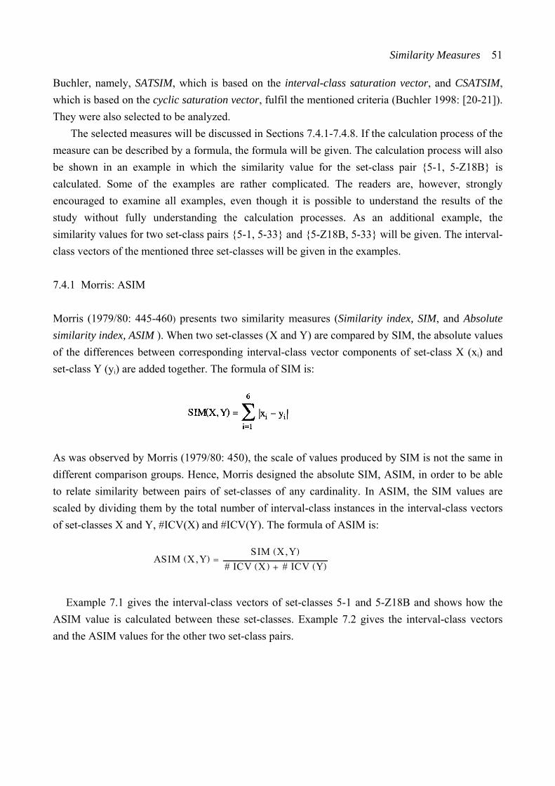
Similarity Measures 51
Buchler, namely, SATSIM, which is based on the interval-class saturation vector, and CSATSIM, which is based on the cyclic saturation vector, fulfil the mentioned criteria (Buchler 1998: [20-21]). They were also selected to be analyzed.
The selected measures will be discussed in Sections 7.4.1-7.4.8. If the calculation process of the measure can be described by a formula, the formula will be given. The calculation process will also be shown in an example in which the similarity value for the set-class pair {5-1, 5-Z18B} is calculated. Some of the examples are rather complicated. The readers are, however, strongly encouraged to examine all examples, even though it is possible to understand the results of the study without fully understanding the calculation processes. As an additional example, the similarity values for two set-class pairs {5-1, 5-33} and {5-Z18B, 5-33} will be given. The interval-class vectors of the mentioned three set-classes will be given in the examples.
7.4.1 Morris: ASIM
Morris (1979/80: 445-460) presents two similarity measures (Similarity index, SIM, and Absolute similarity index, ASIM ). When two set-classes (X and Y) are compared by SIM, the absolute values of the differences between corresponding interval-class vector components of set-class X (xi) and set-class Y (yi) are added together. The formula of SIM is:
As was observed by Morris (1979/80: 450), the scale of values produced by SIM is not the same in different comparison groups. Hence, Morris designed the absolute SIM, ASIM, in order to be able to relate similarity between pairs of set-classes of any cardinality. In ASIM, the SIM values are scaled by dividing them by the total number of interval-class instances in the interval-class vectors of set-classes X and Y, #ICV(X) and #ICV(Y). The formula of ASIM is:
A S I M ( X , Y ) =
S I M ( X , Y ) # I C V ( X ) + # I C V ( Y )
Example 7.1 gives the interval-class vectors of set-classes 5-1 and 5-Z18B and shows how the
ASIM value is calculated between these set-classes. Example 7.2 gives the interval-class vectors and the ASIM values for the other two set-class pairs.
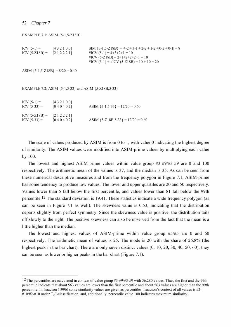
52 Chapter 7
EXAMPLE 7.1: ASIM {5-1,5-Z18B}
ICV (5-1) = [4 3 2 1 0 0] SIM {5-1,5-Z18B} = |4-2|+|3-1|+|2-2|+|1-2|+|0-2|+|0-1| = 8 ICV (5-Z18B) = [2 1 2 2 2 1] #ICV (5-1) = 4+3+2+1 = 10 #ICV (5-Z18B) = 2+1+2+2+2+1 = 10 #ICV (5-1) + #ICV (5-Z18B) = 10 + 10 = 20 ASIM {5-1,5-Z18B} = 8/20 = 0.40 EXAMPLE 7.2: ASIM {5-1,5-33} and ASIM {5-Z18B,5-33} ICV (5-1) = [4 3 2 1 0 0] ICV (5-33) = [0 4 0 4 0 2] ASIM {5-1,5-33} = 12/20 = 0.60 ICV (5-Z18B) = [2 1 2 2 2 1] ICV (5-33) = [0 4 0 4 0 2] ASIM {5-Z18B,5-33} = 12/20 = 0.60
The scale of values produced by ASIM is from 0 to 1, with value 0 indicating the highest degree
of similarity. The ASIM values were modified into ASIM-prime values by multiplying each value by 100.
The lowest and highest ASIM-prime values within value group #3-#9/#3-#9 are 0 and 100 respectively. The arithmetic mean of the values is 37, and the median is 35. As can be seen from these numerical descriptive measures and from the frequency polygon in Figure 7.1, ASIM-prime has some tendency to produce low values. The lower and upper quartiles are 20 and 50 respectively. Values lower than 5 fall below the first percentile, and values lower than 81 fall below the 99th percentile.12 The standard deviation is 19.41. These statistics indicate a wide frequency polygon (as can be seen in Figure 7.1 as well). The skewness value is 0.53, indicating that the distribution departs slightly from perfect symmetry. Since the skewness value is positive, the distribution tails off slowly to the right. The positive skewness can also be observed from the fact that the mean is a little higher than the median.
The lowest and highest values of ASIM-prime within value group #5/#5 are 0 and 60 respectively. The arithmetic mean of values is 25. The mode is 20 with the share of 26.8% (the highest peak in the bar chart). There are only seven distinct values (0, 10, 20, 30, 40, 50, 60); they can be seen as lower or higher peaks in the bar chart (Figure 7.1).
12 The percentiles are calculated in context of value group #3-#9/#3-#9 with 56,280 values. Thus, the first and the 99th percentile indicate that about 563 values are lower than the first percentile and about 563 values are higher than the 99th percentile. In Isaacson (1996) some similarity values are given as percentiles. Isaacson’s context of all values is #2-#10/#2-#10 under Tn/I-classification, and, additionally, percentile value 100 indicates maximum similarity.
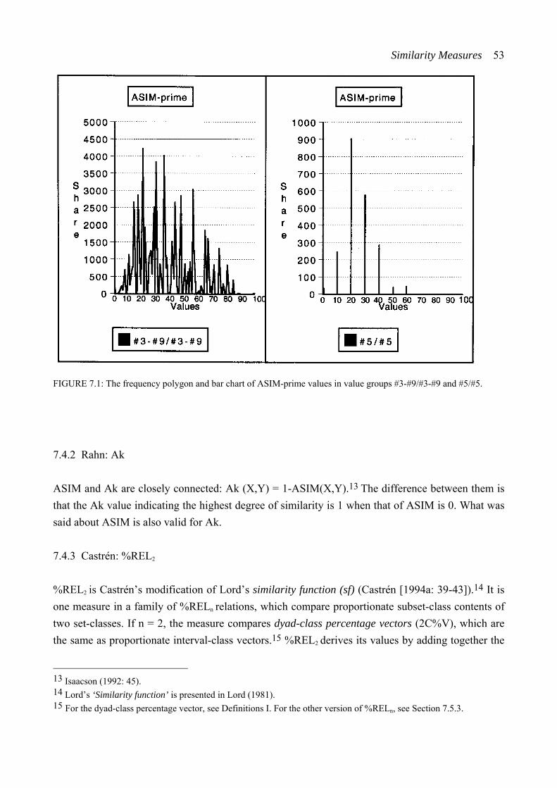
Similarity Measures 53
FIGURE 7.1: The frequency polygon and bar chart of ASIM-prime values in value groups #3-#9/#3-#9 and #5/#5.
7.4.2 Rahn: Ak
ASIM and Ak are closely connected: Ak (X,Y) = 1-ASIM(X,Y).13 The difference between them is that the Ak value indicating the highest degree of similarity is 1 when that of ASIM is 0. What was said about ASIM is also valid for Ak.
7.4.3 Castrén: %REL2
%REL2 is Castrén’s modification of Lord’s similarity function (sf) (Castrén [1994a: 39-43]).14 It is one measure in a family of %RELn relations, which compare proportionate subset-class contents of two set-classes. If n = 2, the measure compares dyad-class percentage vectors (2C%V), which are the same as proportionate interval-class vectors.15 %REL2 derives its values by adding together the
13 Isaacson (1992: 45). 14 Lord’s ‘Similarity function’ is presented in Lord (1981). 15 For the dyad-class percentage vector, see Definitions I. For the other version of %RELn, see Section 7.5.3.
54 Chapter 7
absolute values of differences between corresponding components in the dyad-class percentage vectors of set-classes X and Y (these components are xi and yi respectively) and dividing the sum by two. The formula of %RELn is:
Example 7.3 gives the interval-class vectors and the dyad-class percentage vectors of set-classes
5-1 and 5-Z18B. This example also shows how the %REL2 value is calculated between the set-classes. Example 7.4 gives the %REL2 values for the two additional set-class pairs.
EXAMPLE 7.3: %REL2 {5-1,5-Z18B}
ICV (5-1) = [4 3 2 1 0 0] #ICV(5-1) = 10 2C%V (5-1) = [40 30 20 10 0 0] ICV (5-Z18B) = [2 1 2 2 2 1] #ICV(5-Z18B) = 10 2C%V (5-Z18B) = [20 10 20 20 20 10] %REL2 {5-1,5-Z18B} = ( |40-20|+|30-10|+|20-20|+|10-20|+|0-20|+|0-10| ) / 2 = 80/2 = 40
EXAMPLE 7.4: %REL2 {5-1,5-33}, %REL2 {5-Z18B,5-33}
ICV (5-1) = [4 3 2 1 0 0] ICV (5-33) = [0 4 0 4 0 2] %REL2 {5-1,5-33} = 60 ICV (5-Z18B) = [2 1 2 2 2 1] ICV (5-33) = [0 4 0 4 0 2] %REL2 {5-Z18B,5-33} = 60
The scale of values produced by %REL2 is from 0 (indicating the highest degree of similarity) to
100. Hence, no modification to %REL2-prime was needed. In value group #3-#9/#3-#9 the values lie between 0 and 100, inclusively. The arithmetic mean is
25, and the median is 20. Hence, %REL2 has a rather strong tendency to produce low values. The lower and upper quartiles are 13 and 33 respectively. Values lower than 4 fall below the first percentile and values lower than 76 fall below the 99th percentile. The standard deviation is 16.43. These statistics indicate that the frequency polygon is rather wide. The skewness value is 1.27, indicating that the frequency polygon tails off rather rapidly to the right (see Figure 7.2).
The value group #5/#5 is identical to that of ASIM-prime. There are the same 7 distinct values, the lowest of which is 0 and the highest 60 (see Figure 7.2).
Similarity Measures 55
FIGURE 7.2: The frequency polygon and bar chart of %REL2 values in value groups #3-#9/#3-#9 and #5/#5.
7.4.4 Rogers: IcVD1
Rogers (1992) presents three similarity measures, ‘Distance Formula 1’ (IcVD1), ‘Distance Formula 2’ (IcVD2), and Cosθ.16 These measures are also discussed in detail in Rogers (1999). IcVD1 is a modification of Morris’s SIM (see Section 7.4.1 for SIM) like Castrén’s %REL2 is a modification of Rahn’s Ak (see Section 7.4.3. for %REL2). Their values can be modified to each other by the formula %REL2(X,Y) = IcVD1(X,Y)*50. What was said about %REL2 is also valid for IcVD1.
7.4.5 Rogers: IcVD2
The two other measures by Rogers, IcVD2 and Cosθ, operate with interval-class vectors as with geometric vectors in six-dimensional space (Rogers [1999: 80-81]; for Cosθ, see Section 7.4.6). According to Rogers (1999: 86), IcVD2 measures the distance between the endpoints of two vectors. The idea is that both vectors originate from 0 (the origin of the space) and end at the point defined
16 Rogers (1992) is in three parts; below Rogers (1992 I), (1992 II), and (1992 III).
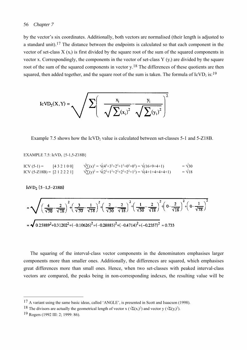
56 Chapter 7
by the vector’s six coordinates. Additionally, both vectors are normalised (their length is adjusted to a standard unit).17 The distance between the endpoints is calculated so that each component in the vector of set-class X (xi) is first divided by the square root of the sum of the squared components in vector x. Correspondingly, the components in the vector of set-class Y (yi) are divided by the square root of the sum of the squared components in vector y.18 The differences of these quotients are then squared, then added together, and the square root of the sum is taken. The formula of IcVD2 is:19
Example 7.5 shows how the IcVD2 value is calculated between set-classes 5-1 and 5-Z18B.
EXAMPLE 7.5: IcVD2 {5-1,5-Z18B} ICV (5-1) = [4 3 2 1 0 0] √∑(x)2 = √(42+32+22+12+02+02) = √(16+9+4+1) = √30 ICV (5-Z18B) = [2 1 2 2 2 1] √∑(y)2 = √(22+12+22+22+22+12) = √(4+1+4+4+4+1) = √18
The squaring of the interval-class vector components in the denominators emphasises larger
components more than smaller ones. Additionally, the differences are squared, which emphasises great differences more than small ones. Hence, when two set-classes with peaked interval-class vectors are compared, the peaks being in non-corresponding indexes, the resulting value will be
17 A variant using the same basic ideas, called ‘ANGLE’, is presented in Scott and Isaacson (1998). 18 The divisors are actually the geometrical length of vector x (√Σ(xi)2) and vector y (√Σ(yi)2). 19 Rogers (1992 III: 2; 1999: 86).
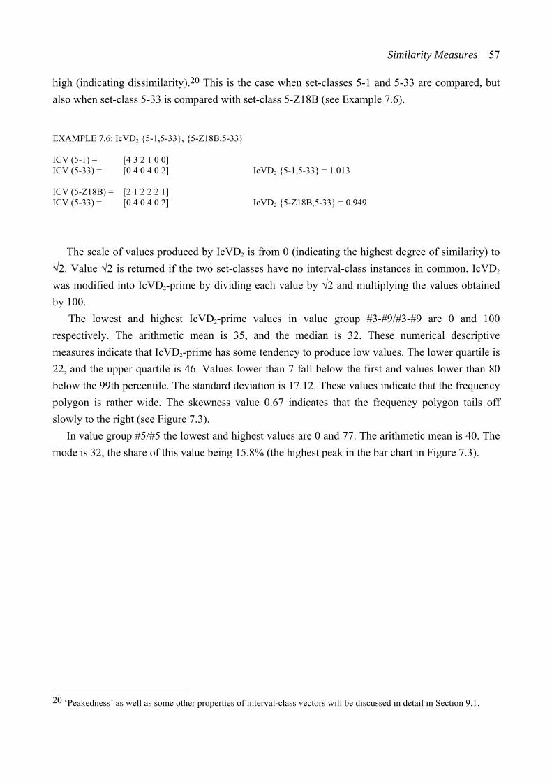
Similarity Measures 57
high (indicating dissimilarity).20 This is the case when set-classes 5-1 and 5-33 are compared, but also when set-class 5-33 is compared with set-class 5-Z18B (see Example 7.6).
EXAMPLE 7.6: IcVD2 {5-1,5-33}, {5-Z18B,5-33} ICV (5-1) = [4 3 2 1 0 0] ICV (5-33) = [0 4 0 4 0 2] IcVD2 {5-1,5-33} = 1.013 ICV (5-Z18B) = [2 1 2 2 2 1] ICV (5-33) = [0 4 0 4 0 2] IcVD2 {5-Z18B,5-33} = 0.949
The scale of values produced by IcVD2 is from 0 (indicating the highest degree of similarity) to
√2. Value √2 is returned if the two set-classes have no interval-class instances in common. IcVD2 was modified into IcVD2-prime by dividing each value by √2 and multiplying the values obtained by 100.
The lowest and highest IcVD2-prime values in value group #3-#9/#3-#9 are 0 and 100 respectively. The arithmetic mean is 35, and the median is 32. These numerical descriptive measures indicate that IcVD2-prime has some tendency to produce low values. The lower quartile is 22, and the upper quartile is 46. Values lower than 7 fall below the first and values lower than 80 below the 99th percentile. The standard deviation is 17.12. These values indicate that the frequency polygon is rather wide. The skewness value 0.67 indicates that the frequency polygon tails off slowly to the right (see Figure 7.3).
In value group #5/#5 the lowest and highest values are 0 and 77. The arithmetic mean is 40. The mode is 32, the share of this value being 15.8% (the highest peak in the bar chart in Figure 7.3).
20 ‘Peakedness’ as well as some other properties of interval-class vectors will be discussed in detail in Section 9.1.
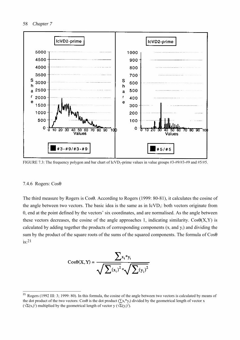
58 Chapter 7
FIGURE 7.3: The frequency polygon and bar chart of IcVD2-prime values in value groups #3-#9/#3-#9 and #5/#5.
7.4.6 Rogers: Cosθ
The third measure by Rogers is Cosθ. According to Rogers (1999: 80-81), it calculates the cosine of the angle between two vectors. The basic idea is the same as in IcVD2: both vectors originate from 0, end at the point defined by the vectors’ six coordinates, and are normalised. As the angle between these vectors decreases, the cosine of the angle approaches 1, indicating similarity. Cosθ(X,Y) is calculated by adding together the products of corresponding components (xi and yi) and dividing the sum by the product of the square roots of the sums of the squared components. The formula of Cosθ is:21
21 Rogers (1992 III: 3; 1999: 80). In this formula, the cosine of the angle between two vectors is calculated by means of the dot product of the two vectors: Cosθ is the dot product (∑xi*yi) divided by the geometrical length of vector x (√Σ(xi)2) multiplied by the geometrical length of vector y (√Σ(yi)2).
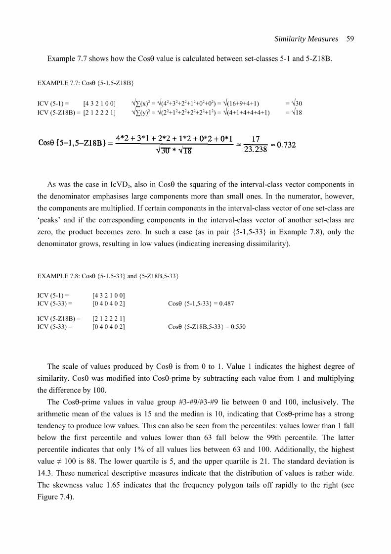
Similarity Measures 59
Example 7.7 shows how the Cosθ value is calculated between set-classes 5-1 and 5-Z18B.
EXAMPLE 7.7: Cosθ {5-1,5-Z18B}
ICV (5-1) = [4 3 2 1 0 0] √∑(x)2 = √(42+32+22+12+02+02) = √(16+9+4+1) = √30 ICV (5-Z18B) = [2 1 2 2 2 1] √∑(y)2 = √(22+12+22+22+22+12) = √(4+1+4+4+4+1) = √18
As was the case in IcVD2, also in Cosθ the squaring of the interval-class vector components in the denominator emphasises large components more than small ones. In the numerator, however, the components are multiplied. If certain components in the interval-class vector of one set-class are ‘peaks’ and if the corresponding components in the interval-class vector of another set-class are zero, the product becomes zero. In such a case (as in pair {5-1,5-33} in Example 7.8), only the denominator grows, resulting in low values (indicating increasing dissimilarity).
EXAMPLE 7.8: Cosθ {5-1,5-33} and {5-Z18B,5-33}
ICV (5-1) = [4 3 2 1 0 0] ICV (5-33) = [0 4 0 4 0 2] Cosθ {5-1,5-33} = 0.487 ICV (5-Z18B) = [2 1 2 2 2 1] ICV (5-33) = [0 4 0 4 0 2] Cosθ {5-Z18B,5-33} = 0.550
The scale of values produced by Cosθ is from 0 to 1. Value 1 indicates the highest degree of similarity. Cosθ was modified into Cosθ-prime by subtracting each value from 1 and multiplying the difference by 100.
The Cosθ-prime values in value group #3-#9/#3-#9 lie between 0 and 100, inclusively. The arithmetic mean of the values is 15 and the median is 10, indicating that Cosθ-prime has a strong tendency to produce low values. This can also be seen from the percentiles: values lower than 1 fall below the first percentile and values lower than 63 fall below the 99th percentile. The latter percentile indicates that only 1% of all values lies between 63 and 100. Additionally, the highest value ≠ 100 is 88. The lower quartile is 5, and the upper quartile is 21. The standard deviation is 14.3. These numerical descriptive measures indicate that the distribution of values is rather wide. The skewness value 1.65 indicates that the frequency polygon tails off rapidly to the right (see Figure 7.4).
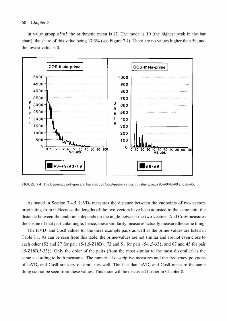
60 Chapter 7
In value group #5/#5 the arithmetic mean is 17. The mode is 10 (the highest peak in the bar chart), the share of this value being 17.3% (see Figure 7.4). There are no values higher than 59, and the lowest value is 0.
FIGURE 7.4: The frequency polygon and bar chart of Cosθ-prime values in value groups #3-#9/#3-#9 and #5/#5. As stated in Section 7.4.5, IcVD2 measures the distance between the endpoints of two vectors
originating from 0. Because the lengths of the two vectors have been adjusted to the same unit, the distance between the endpoints depends on the angle between the two vectors. And Cosθ measures the cosine of that particular angle; hence, these similarity measures actually measure the same thing.
The IcVD2 and Cosθ values for the three example pairs as well as the prime-values are listed in Table 7.1. As can be seen from this table, the prime-values are not similar and are not even close to each other (52 and 27 for pair {5-1,5-Z18B}, 72 and 51 for pair {5-1,5-33}, and 67 and 45 for pair {5-Z18B,5-33}). Only the order of the pairs (from the most similar to the most dissimilar) is the same according to both measures. The numerical descriptive measures and the frequency polygons of IcVD2 and Cosθ are very dissimilar as well. The fact that IcVD2 and Cosθ measure the same thing cannot be seen from these values. This issue will be discussed further in Chapter 8.
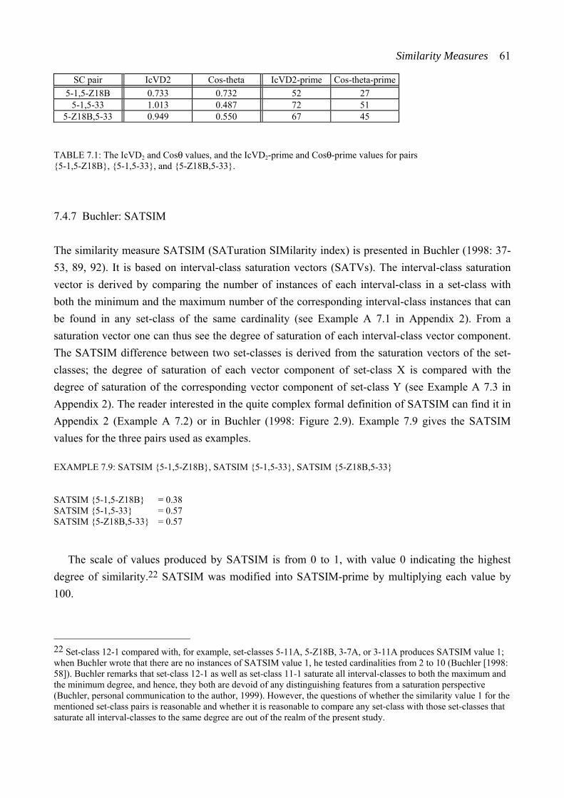
Similarity Measures 61
SC pair IcVD2 Cos-theta IcVD2-prime Cos-theta-prime5-1,5-Z18B 0.733 0.732 52 27
5-1,5-33 1.013 0.487 72 51 5-Z18B,5-33 0.949 0.550 67 45
TABLE 7.1: The IcVD2 and Cosθ values, and the IcVD2-prime and Cosθ-prime values for pairs {5-1,5-Z18B}, {5-1,5-33}, and {5-Z18B,5-33}.
7.4.7 Buchler: SATSIM
The similarity measure SATSIM (SATuration SIMilarity index) is presented in Buchler (1998: 37-53, 89, 92). It is based on interval-class saturation vectors (SATVs). The interval-class saturation vector is derived by comparing the number of instances of each interval-class in a set-class with both the minimum and the maximum number of the corresponding interval-class instances that can be found in any set-class of the same cardinality (see Example A 7.1 in Appendix 2). From a saturation vector one can thus see the degree of saturation of each interval-class vector component. The SATSIM difference between two set-classes is derived from the saturation vectors of the set-classes; the degree of saturation of each vector component of set-class X is compared with the degree of saturation of the corresponding vector component of set-class Y (see Example A 7.3 in Appendix 2). The reader interested in the quite complex formal definition of SATSIM can find it in Appendix 2 (Example A 7.2) or in Buchler (1998: Figure 2.9). Example 7.9 gives the SATSIM values for the three pairs used as examples.
EXAMPLE 7.9: SATSIM {5-1,5-Z18B}, SATSIM {5-1,5-33}, SATSIM {5-Z18B,5-33}
SATSIM {5-1,5-Z18B} = 0.38 SATSIM {5-1,5-33} = 0.57 SATSIM {5-Z18B,5-33} = 0.57
The scale of values produced by SATSIM is from 0 to 1, with value 0 indicating the highest degree of similarity.22 SATSIM was modified into SATSIM-prime by multiplying each value by 100.
22 Set-class 12-1 compared with, for example, set-classes 5-11A, 5-Z18B, 3-7A, or 3-11A produces SATSIM value 1; when Buchler wrote that there are no instances of SATSIM value 1, he tested cardinalities from 2 to 10 (Buchler [1998: 58]). Buchler remarks that set-class 12-1 as well as set-class 11-1 saturate all interval-classes to both the maximum and the minimum degree, and hence, they both are devoid of any distinguishing features from a saturation perspective (Buchler, personal communication to the author, 1999). However, the questions of whether the similarity value 1 for the mentioned set-class pairs is reasonable and whether it is reasonable to compare any set-class with those set-classes that saturate all interval-classes to the same degree are out of the realm of the present study.
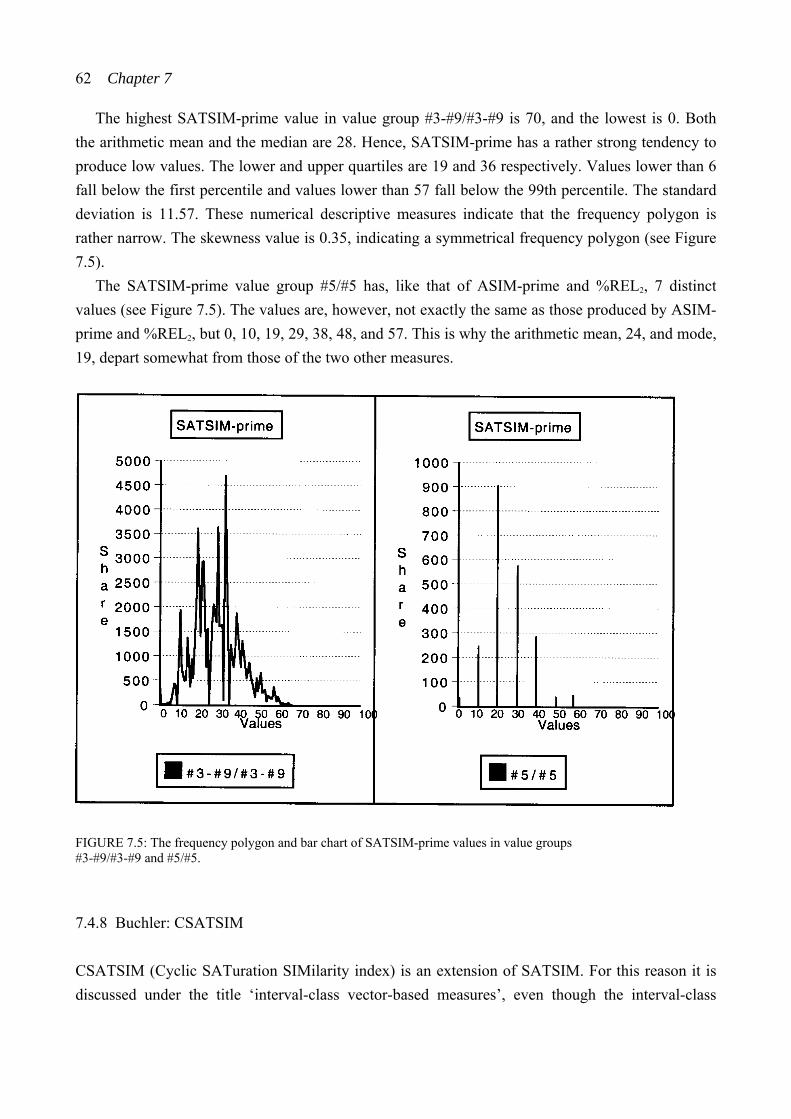
62 Chapter 7
The highest SATSIM-prime value in value group #3-#9/#3-#9 is 70, and the lowest is 0. Both the arithmetic mean and the median are 28. Hence, SATSIM-prime has a rather strong tendency to produce low values. The lower and upper quartiles are 19 and 36 respectively. Values lower than 6 fall below the first percentile and values lower than 57 fall below the 99th percentile. The standard deviation is 11.57. These numerical descriptive measures indicate that the frequency polygon is rather narrow. The skewness value is 0.35, indicating a symmetrical frequency polygon (see Figure 7.5).
The SATSIM-prime value group #5/#5 has, like that of ASIM-prime and %REL2, 7 distinct values (see Figure 7.5). The values are, however, not exactly the same as those produced by ASIM-prime and %REL2, but 0, 10, 19, 29, 38, 48, and 57. This is why the arithmetic mean, 24, and mode, 19, depart somewhat from those of the two other measures.
FIGURE 7.5: The frequency polygon and bar chart of SATSIM-prime values in value groups #3-#9/#3-#9 and #5/#5.
7.4.8 Buchler: CSATSIM
CSATSIM (Cyclic SATuration SIMilarity index) is an extension of SATSIM. For this reason it is discussed under the title ‘interval-class vector-based measures’, even though the interval-class
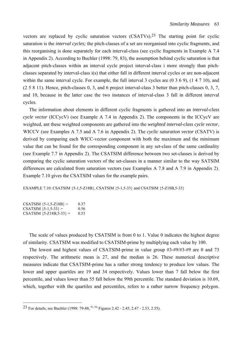
Similarity Measures 63
vectors are replaced by cyclic saturation vectors (CSATVs).23 The starting point for cyclic saturation is the interval cycles; the pitch-classes of a set are reorganised into cyclic fragments, and this reorganising is done separately for each interval-class (see cyclic fragments in Example A 7.4 in Appendix 2). According to Buchler (1998: 79, 83), the assumption behind cyclic saturation is that adjacent pitch-classes within an interval cycle project interval-class i more strongly than pitch-classes separated by interval-class i(s) that either fall in different interval cycles or are non-adjacent within the same interval cycle. For example, the full interval 3 cycles are (0 3 6 9), (1 4 7 10), and (2 5 8 11). Hence, pitch-classes 0, 3, and 6 project interval-class 3 better than pitch-classes 0, 3, 7, and 10, because in the latter case the two instances of interval-class 3 fall in different interval cycles.
The information about elements in different cyclic fragments is gathered into an interval-class cycle vector (ICCycV) (see Example A 7.4 in Appendix 2). The components in the ICCycV are
weighted, ant these weighted components are gathered into the weighted interval-class cycle vector, WICCV (see Examples A 7.5 and A 7.6 in Appendix 2). The cyclic saturation vector (CSATV) is derived by comparing each WICC-vector component with both the maximum and the minimum value that can be found for the corresponding component in any set-class of the same cardinality (see Example 7.7 in Appendix 2). The CSATSIM difference between two set-classes is derived by comparing the cyclic saturation vectors of the set-classes in a manner similar to the way SATSIM differences are calculated from saturation vectors (see Examples A 7.8 and A 7.9 in Appendix 2).
Example 7.10 gives the CSATSIM values for the example pairs.
EXAMPLE 7.10: CSATSIM {5-1,5-Z18B}, CSATSIM {5-1,5-33} and CSATSIM {5-Z18B,5-33} CSATSIM {5-1,5-Z18B} = 0.37 CSATSIM {5-1,5-33} = 0.56 CSATSIM {5-Z18B,5-33} = 0.53
The scale of values produced by CSATSIM is from 0 to 1. Value 0 indicates the highest degree of similarity. CSATSIM was modified to CSATSIM-prime by multiplying each value by 100.
The lowest and highest values of CSATSIM-prime in value group #3-#9/#3-#9 are 0 and 73 respectively. The arithmetic mean is 27, and the median is 26. These numerical descriptive measures indicate that CSATSIM-prime has a rather strong tendency to produce low values. The lower and upper quartiles are 19 and 34 respectively. Values lower than 7 fall below the first percentile, and values lower than 55 fall below the 99th percentile. The standard deviation is 10.69, which, together with the quartiles and percentiles, refers to a rather narrow frequency polygon.
23 For details, see Buchler (1998: 79-88, 91, 94, Figures 2.42 - 2.45, 2.47 - 2.53, 2.55).
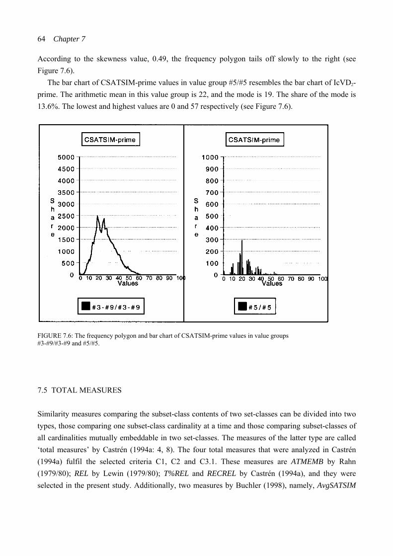
64 Chapter 7
According to the skewness value, 0.49, the frequency polygon tails off slowly to the right (see Figure 7.6).
The bar chart of CSATSIM-prime values in value group #5/#5 resembles the bar chart of IcVD2-prime. The arithmetic mean in this value group is 22, and the mode is 19. The share of the mode is 13.6%. The lowest and highest values are 0 and 57 respectively (see Figure 7.6).
FIGURE 7.6: The frequency polygon and bar chart of CSATSIM-prime values in value groups #3-#9/#3-#9 and #5/#5.
7.5 TOTAL MEASURES
Similarity measures comparing the subset-class contents of two set-classes can be divided into two types, those comparing one subset-class cardinality at a time and those comparing subset-classes of all cardinalities mutually embeddable in two set-classes. The measures of the latter type are called ‘total measures’ by Castrén (1994a: 4, 8). The four total measures that were analyzed in Castrén (1994a) fulfil the selected criteria C1, C2 and C3.1. These measures are ATMEMB by Rahn (1979/80); REL by Lewin (1979/80); T%REL and RECREL by Castrén (1994a), and they were selected in the present study. Additionally, two measures by Buchler (1998), namely, AvgSATSIM
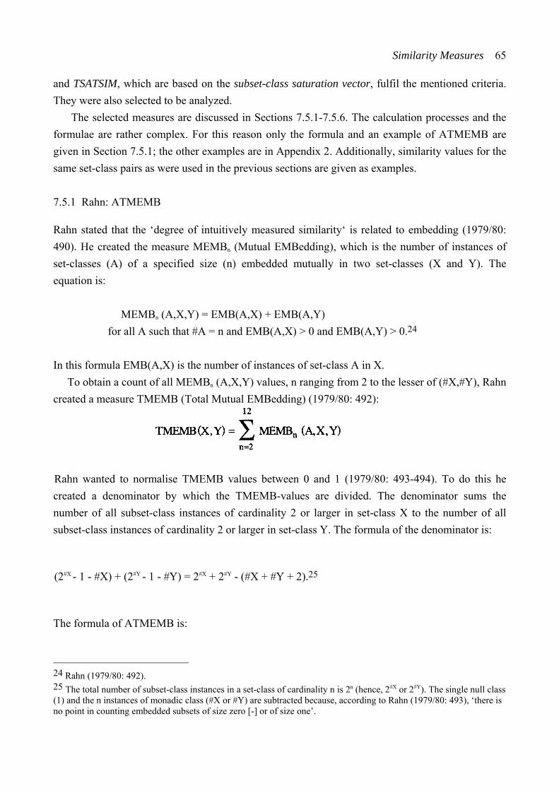
Similarity Measures 65
and TSATSIM, which are based on the subset-class saturation vector, fulfil the mentioned criteria. They were also selected to be analyzed.
The selected measures are discussed in Sections 7.5.1-7.5.6. The calculation processes and the formulae are rather complex. For this reason only the formula and an example of ATMEMB are given in Section 7.5.1; the other examples are in Appendix 2. Additionally, similarity values for the same set-class pairs as were used in the previous sections are given as examples.
7.5.1 Rahn: ATMEMB
Rahn stated that the ‘degree of intuitively measured similarity‘ is related to embedding (1979/80: 490). He created the measure MEMBn (Mutual EMBedding), which is the number of instances of set-classes (A) of a specified size (n) embedded mutually in two set-classes (X and Y). The equation is:
MEMBn (A,X,Y) = EMB(A,X) + EMB(A,Y) for all A such that #A = n and EMB(A,X) > 0 and EMB(A,Y) > 0.24
In this formula EMB(A,X) is the number of instances of set-class A in X.
To obtain a count of all MEMBn (A,X,Y) values, n ranging from 2 to the lesser of (#X,#Y), Rahn created a measure TMEMB (Total Mutual EMBedding) (1979/80: 492):
Rahn wanted to normalise TMEMB values between 0 and 1 (1979/80: 493-494). To do this he created a denominator by which the TMEMB-values are divided. The denominator sums the number of all subset-class instances of cardinality 2 or larger in set-class X to the number of all subset-class instances of cardinality 2 or larger in set-class Y. The formula of the denominator is: (2#X - 1 - #X) + (2#Y - 1 - #Y) = 2#X + 2#Y - (#X + #Y + 2).25
The formula of ATMEMB is:
24 Rahn (1979/80: 492). 25 The total number of subset-class instances in a set-class of cardinality n is 2n (hence, 2#X or 2#Y). The single null class (1) and the n instances of monadic class (#X or #Y) are subtracted because, according to Rahn (1979/80: 493), ‘there is no point in counting embedded subsets of size zero [-] or of size one’.
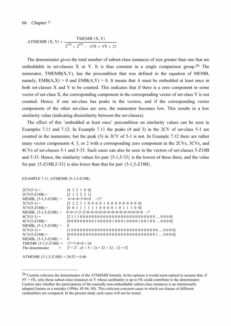
66 Chapter 7
A T M E M B ( X , Y ) =
T M E M B ( X , Y )
2 # X + 2 # Y − ( # X + # Y + 2 ) The denominator gives the total number of subset-class instances of size greater than one that are
embeddable in set-classes X or Y. It is thus constant in a single comparison group.26 The numerator, TMEMB(X,Y), has the precondition that was defined in the equation of MEMB, namely, EMB(A,X) > 0 and EMB(A,Y) > 0. It means that A must be embedded at least once in both set-classes X and Y to be counted. This indicates that if there is a zero component in some vector of set-class X, the corresponding component in the corresponding vector of set-class Y is not counted. Hence, if one set-class has peaks in the vectors, and if the corresponding vector components of the other set-class are zero, the numerator becomes low. This results in a low similarity value (indicating dissimilarity between the set-classes).
The effect of this ‘embedded at least once’ precondition on similarity values can be seen in Examples 7.11 and 7.12. In Example 7.11 the peaks (4 and 3) in the 2CV of set-class 5-1 are counted in the numerator, but the peak (3) in 3CV of 5-1 is not. In Example 7.12 there are rather many vector components 4, 3, or 2 with a corresponding zero component in the 2CVs, 3CVs, and 4CVs of set-classes 5-1 and 5-33. Such cases can also be seen in the vectors of set-classes 5-Z18B and 5-33. Hence, the similarity values for pair {5-1,5-33} is the lowest of these three, and the value for pair {5-Z18B,5-33} is also lower than that for pair {5-1,5-Z18B}.
EXAMPLE 7.11: ATMEMB {5-1,5-Z18B}
2CV(5-1) = [4 3 2 1 0 0] 2CV(5-Z18B) = [2 1 2 2 2 1] MEMB2 {5-1,5-Z18B} = 6+4+4+3+0+0 =17 3CV(5-1) = [3 2 2 1 1 0 0 0 0 1 0 0 0 0 0 0 0 0 0] 3CV(5-Z18B) = [0 0 1 1 1 1 1 1 0 0 0 0 1 0 1 1 1 0 0] MEMB3 {5-1,5-Z18B} = 0+0+3+2+2+0+0+0+0+0+0+0+0+0+0+0+0+0+0 =7 4CV(5-1) = [2 1 1 1 0 0 0 0 0 0 0 0 0 0 0 0 0 0 0 0 0 0 0 0 0 0 0 0 0 0 .... 0 0 0 0] 4CV(5-Z18B) = [0 0 0 0 0 0 0 0 0 1 0 0 0 0 0 1 0 0 0 1 0 0 0 0 1 0 0 1 0 0 .... 0 0 0 0] MEMB4 {5-1,5-Z18B} = 0 5CV(5-1) = [1 0 0 0 0 0 0 0 0 0 0 0 0 0 0 0 0 0 0 0 0 0 0 0 0 0 0 0 0 0 0 .... 0 0 0 0] 5CV(5-Z18B) = [0 0 0 0 0 0 0 0 0 0 0 0 0 0 0 0 0 0 0 0 0 0 0 0 0 0 0 0 0 0 1 .... 0 0 0 0] MEMB5 {5-1,5-Z18B} = 0 TMEMB {5-1,5-Z18B} = 17+7+0+0 = 24 The denominator = 25 + 25 - (5 + 5 + 2) = 32 + 32 - 12 = 52 ATMEMB {5-1,5-Z18B} = 24/52 = 0.46
26 Castrén criticises the denominator of the ATMEMB formula. In his opinion it would seem natural to assume that, if #Y > #X, only those subset-class instances in Y whose cardinality is up to #X could contribute to the denominator. Castrén asks whether the participation of the mutually non-embeddable subset-class instances is an intentionally adopted feature or a mistake (1994a: 85-86, 89). This criticism concerns cases in which set-classes of different cardinalities are compared. In the present study such cases will not be tested.
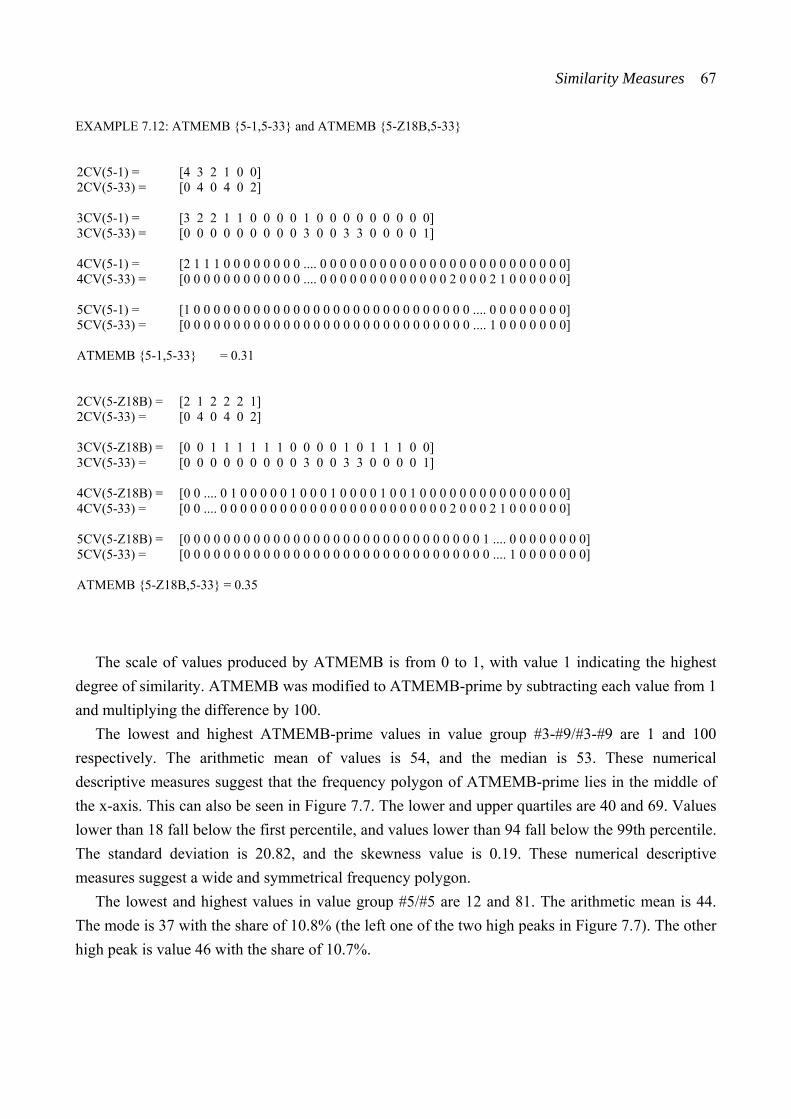
Similarity Measures 67
EXAMPLE 7.12: ATMEMB {5-1,5-33} and ATMEMB {5-Z18B,5-33} 2CV(5-1) = [4 3 2 1 0 0] 2CV(5-33) = [0 4 0 4 0 2] 3CV(5-1) = [3 2 2 1 1 0 0 0 0 1 0 0 0 0 0 0 0 0 0] 3CV(5-33) = [0 0 0 0 0 0 0 0 0 3 0 0 3 3 0 0 0 0 1] 4CV(5-1) = [2 1 1 1 0 0 0 0 0 0 0 0 .... 0 0 0 0 0 0 0 0 0 0 0 0 0 0 0 0 0 0 0 0 0 0 0 0 0] 4CV(5-33) = [0 0 0 0 0 0 0 0 0 0 0 0 .... 0 0 0 0 0 0 0 0 0 0 0 0 0 2 0 0 0 2 1 0 0 0 0 0 0] 5CV(5-1) = [1 0 0 0 0 0 0 0 0 0 0 0 0 0 0 0 0 0 0 0 0 0 0 0 0 0 0 0 0 .... 0 0 0 0 0 0 0 0] 5CV(5-33) = [0 0 0 0 0 0 0 0 0 0 0 0 0 0 0 0 0 0 0 0 0 0 0 0 0 0 0 0 0 .... 1 0 0 0 0 0 0 0] ATMEMB {5-1,5-33} = 0.31 2CV(5-Z18B) = [2 1 2 2 2 1] 2CV(5-33) = [0 4 0 4 0 2] 3CV(5-Z18B) = [0 0 1 1 1 1 1 1 0 0 0 0 1 0 1 1 1 0 0] 3CV(5-33) = [0 0 0 0 0 0 0 0 0 3 0 0 3 3 0 0 0 0 1] 4CV(5-Z18B) = [0 0 .... 0 1 0 0 0 0 0 1 0 0 0 1 0 0 0 0 1 0 0 1 0 0 0 0 0 0 0 0 0 0 0 0 0 0 0] 4CV(5-33) = [0 0 .... 0 0 0 0 0 0 0 0 0 0 0 0 0 0 0 0 0 0 0 0 0 0 0 2 0 0 0 2 1 0 0 0 0 0 0] 5CV(5-Z18B) = [0 0 0 0 0 0 0 0 0 0 0 0 0 0 0 0 0 0 0 0 0 0 0 0 0 0 0 0 0 0 1 .... 0 0 0 0 0 0 0 0] 5CV(5-33) = [0 0 0 0 0 0 0 0 0 0 0 0 0 0 0 0 0 0 0 0 0 0 0 0 0 0 0 0 0 0 0 .... 1 0 0 0 0 0 0 0] ATMEMB {5-Z18B,5-33} = 0.35
The scale of values produced by ATMEMB is from 0 to 1, with value 1 indicating the highest
degree of similarity. ATMEMB was modified to ATMEMB-prime by subtracting each value from 1 and multiplying the difference by 100.
The lowest and highest ATMEMB-prime values in value group #3-#9/#3-#9 are 1 and 100 respectively. The arithmetic mean of values is 54, and the median is 53. These numerical descriptive measures suggest that the frequency polygon of ATMEMB-prime lies in the middle of the x-axis. This can also be seen in Figure 7.7. The lower and upper quartiles are 40 and 69. Values lower than 18 fall below the first percentile, and values lower than 94 fall below the 99th percentile. The standard deviation is 20.82, and the skewness value is 0.19. These numerical descriptive measures suggest a wide and symmetrical frequency polygon.
The lowest and highest values in value group #5/#5 are 12 and 81. The arithmetic mean is 44. The mode is 37 with the share of 10.8% (the left one of the two high peaks in Figure 7.7). The other high peak is value 46 with the share of 10.7%.
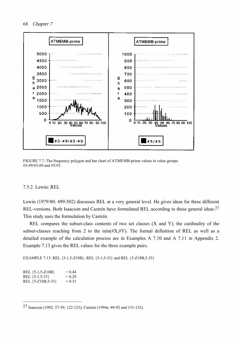
68 Chapter 7
FIGURE 7.7: The frequency polygon and bar chart of ATMEMB-prime values in value groups #3-#9/#3-#9 and #5/#5.
7.5.2 Lewin: REL
Lewin (1979/80: 499-502) discusses REL at a very general level. He gives ideas for three different REL-versions. Both Isaacson and Castrén have formulated REL according to these general ideas.27 This study uses the formulation by Castrén.
REL compares the subset-class contents of two set classes (X and Y), the cardinality of the subset-classes reaching from 2 to the min(#X,#Y). The formal definition of REL as well as a detailed example of the calculation process are in Examples A 7.10 and A 7.11 in Appendix 2. Example 7.13 gives the REL values for the three example pairs.
EXAMPLE 7.13: REL {5-1,5-Z18B}, REL {5-1,5-33} and REL {5-Z18B,5-33} REL {5-1,5-Z18B} = 0.44 REL {5-1,5-33} = 0.28 REL {5-Z18B,5-33} = 0.31
27 Isaacson (1992: 57-59, 122-123); Castrén (1994a: 89-92 and 131-132).
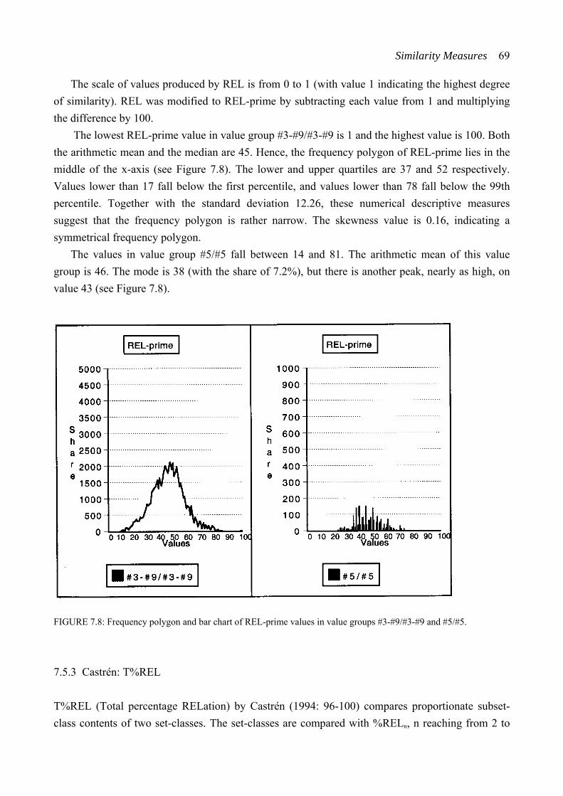
Similarity Measures 69
The scale of values produced by REL is from 0 to 1 (with value 1 indicating the highest degree of similarity). REL was modified to REL-prime by subtracting each value from 1 and multiplying the difference by 100.
The lowest REL-prime value in value group #3-#9/#3-#9 is 1 and the highest value is 100. Both the arithmetic mean and the median are 45. Hence, the frequency polygon of REL-prime lies in the middle of the x-axis (see Figure 7.8). The lower and upper quartiles are 37 and 52 respectively. Values lower than 17 fall below the first percentile, and values lower than 78 fall below the 99th percentile. Together with the standard deviation 12.26, these numerical descriptive measures suggest that the frequency polygon is rather narrow. The skewness value is 0.16, indicating a symmetrical frequency polygon.
The values in value group #5/#5 fall between 14 and 81. The arithmetic mean of this value group is 46. The mode is 38 (with the share of 7.2%), but there is another peak, nearly as high, on value 43 (see Figure 7.8).
FIGURE 7.8: Frequency polygon and bar chart of REL-prime values in value groups #3-#9/#3-#9 and #5/#5.
7.5.3 Castrén: T%REL
T%REL (Total percentage RELation) by Castrén (1994: 96-100) compares proportionate subset-class contents of two set-classes. The set-classes are compared with %RELn, n reaching from 2 to
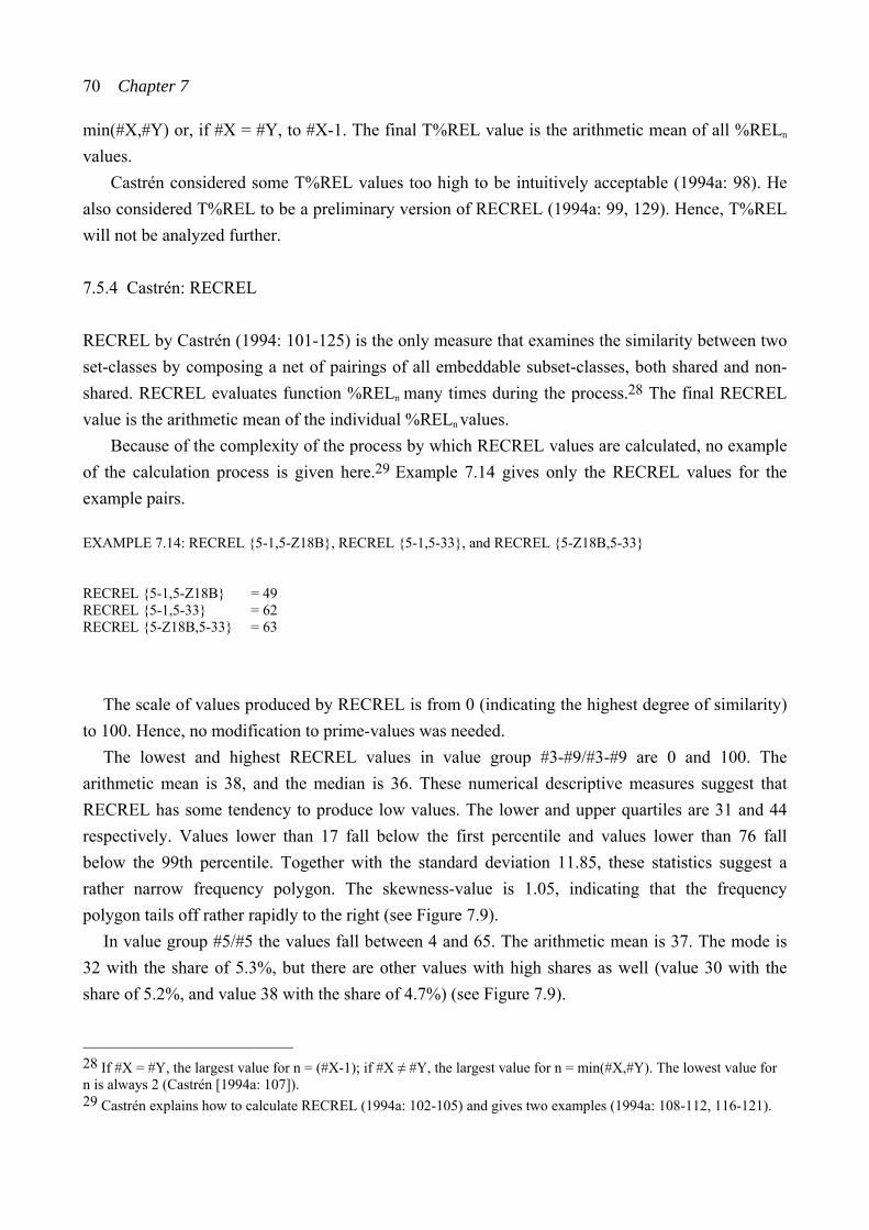
70 Chapter 7
min(#X,#Y) or, if #X = #Y, to #X-1. The final T%REL value is the arithmetic mean of all %RELn values.
Castrén considered some T%REL values too high to be intuitively acceptable (1994a: 98). He also considered T%REL to be a preliminary version of RECREL (1994a: 99, 129). Hence, T%REL will not be analyzed further.
7.5.4 Castrén: RECREL
RECREL by Castrén (1994: 101-125) is the only measure that examines the similarity between two set-classes by composing a net of pairings of all embeddable subset-classes, both shared and non-shared. RECREL evaluates function %RELn many times during the process.28 The final RECREL value is the arithmetic mean of the individual %RELn values.
Because of the complexity of the process by which RECREL values are calculated, no example of the calculation process is given here.29 Example 7.14 gives only the RECREL values for the example pairs.
EXAMPLE 7.14: RECREL {5-1,5-Z18B}, RECREL {5-1,5-33}, and RECREL {5-Z18B,5-33}
RECREL {5-1,5-Z18B} = 49 RECREL {5-1,5-33} = 62 RECREL {5-Z18B,5-33} = 63
The scale of values produced by RECREL is from 0 (indicating the highest degree of similarity)
to 100. Hence, no modification to prime-values was needed. The lowest and highest RECREL values in value group #3-#9/#3-#9 are 0 and 100. The
arithmetic mean is 38, and the median is 36. These numerical descriptive measures suggest that RECREL has some tendency to produce low values. The lower and upper quartiles are 31 and 44 respectively. Values lower than 17 fall below the first percentile and values lower than 76 fall below the 99th percentile. Together with the standard deviation 11.85, these statistics suggest a rather narrow frequency polygon. The skewness-value is 1.05, indicating that the frequency polygon tails off rather rapidly to the right (see Figure 7.9).
In value group #5/#5 the values fall between 4 and 65. The arithmetic mean is 37. The mode is 32 with the share of 5.3%, but there are other values with high shares as well (value 30 with the share of 5.2%, and value 38 with the share of 4.7%) (see Figure 7.9).
28 If #X = #Y, the largest value for n = (#X-1); if #X ≠ #Y, the largest value for n = min(#X,#Y). The lowest value for n is always 2 (Castrén [1994a: 107]). 29 Castrén explains how to calculate RECREL (1994a: 102-105) and gives two examples (1994a: 108-112, 116-121).
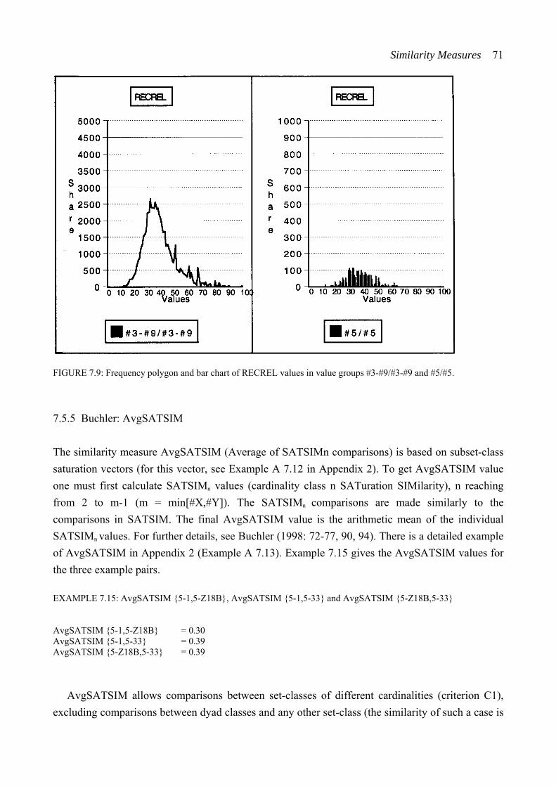
Similarity Measures 71
FIGURE 7.9: Frequency polygon and bar chart of RECREL values in value groups #3-#9/#3-#9 and #5/#5.
7.5.5 Buchler: AvgSATSIM
The similarity measure AvgSATSIM (Average of SATSIMn comparisons) is based on subset-class saturation vectors (for this vector, see Example A 7.12 in Appendix 2). To get AvgSATSIM value one must first calculate SATSIMn values (cardinality class n SATuration SIMilarity), n reaching from 2 to m-1 (m = min[#X,#Y]). The SATSIMn comparisons are made similarly to the comparisons in SATSIM. The final AvgSATSIM value is the arithmetic mean of the individual SATSIMn values. For further details, see Buchler (1998: 72-77, 90, 94). There is a detailed example of AvgSATSIM in Appendix 2 (Example A 7.13). Example 7.15 gives the AvgSATSIM values for the three example pairs.
EXAMPLE 7.15: AvgSATSIM {5-1,5-Z18B}, AvgSATSIM {5-1,5-33} and AvgSATSIM {5-Z18B,5-33} AvgSATSIM {5-1,5-Z18B} = 0.30 AvgSATSIM {5-1,5-33} = 0.39 AvgSATSIM {5-Z18B,5-33} = 0.39
AvgSATSIM allows comparisons between set-classes of different cardinalities (criterion C1),
excluding comparisons between dyad classes and any other set-class (the similarity of such a case is
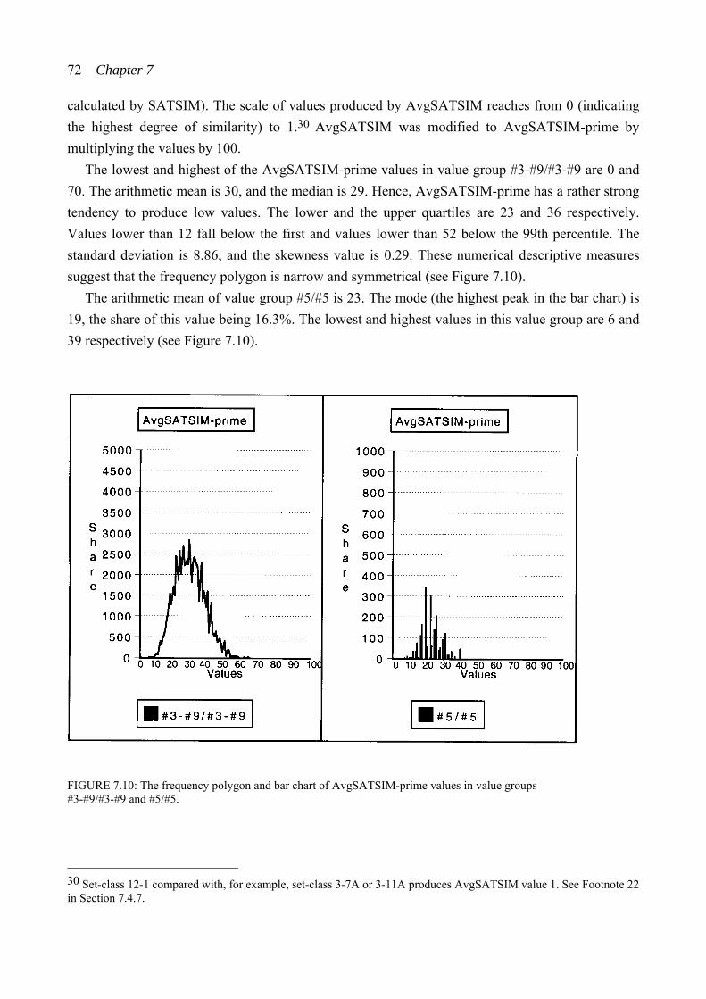
72 Chapter 7
calculated by SATSIM). The scale of values produced by AvgSATSIM reaches from 0 (indicating the highest degree of similarity) to 1.30 AvgSATSIM was modified to AvgSATSIM-prime by multiplying the values by 100.
The lowest and highest of the AvgSATSIM-prime values in value group #3-#9/#3-#9 are 0 and 70. The arithmetic mean is 30, and the median is 29. Hence, AvgSATSIM-prime has a rather strong tendency to produce low values. The lower and the upper quartiles are 23 and 36 respectively. Values lower than 12 fall below the first and values lower than 52 below the 99th percentile. The standard deviation is 8.86, and the skewness value is 0.29. These numerical descriptive measures suggest that the frequency polygon is narrow and symmetrical (see Figure 7.10).
The arithmetic mean of value group #5/#5 is 23. The mode (the highest peak in the bar chart) is 19, the share of this value being 16.3%. The lowest and highest values in this value group are 6 and 39 respectively (see Figure 7.10).
FIGURE 7.10: The frequency polygon and bar chart of AvgSATSIM-prime values in value groups #3-#9/#3-#9 and #5/#5.
30 Set-class 12-1 compared with, for example, set-class 3-7A or 3-11A produces AvgSATSIM value 1. See Footnote 22 in Section 7.4.7.

Similarity Measures 73
7.5.6 Buchler: TSATSIM
The similarity measure TSATSIM (Total subset SATuration SIMilarity index) by Buchler (1998: 76-77, 93) differs only slightly from AvgSATSIM. It is also based on SATSIMn values, n reaching from 2 to m-1 (m = min[#X,#Y]). The final TSATSIM value is calculated by dividing the sum of the numerators of all SATSIMn comparisons by the sum of the denominators. The values produced by TSATSIM are very close to those produced by AvgSATSIM.31 Hence, AvgSATSIM will represent both measures here.
31 See Buchler (1998: Figures 2.40 and 2.41).
CHAPTER EIGHT COMPARING MEASURED SIMILARITY VALUES
In this chapter, the values produced by the ten similarity measures selected in Chapter 7 will be discussed. All values are to be given on the scale from 0 to 100, value 0 indicating maximum similarity. As was done in Chapter 7, the symbol ‘prime’ is used in the names of measures that are modified to produce values on this scale. It should be remembered that two measures, %REL2 and RECREL, already in their original form produce values on this scale and, hence, will not have the prime symbol. Section 8.1 compares the prime values for the three set-class pairs that were used as example pairs in the previous chapter. It will be shown that even with the uniform scale of values, it is not possible to compare values produced by different measures without serious problems, because the distributions of values differ so much from one measure to another (the distributions of values were analyzed in Chapter 7). Consequently, another modification will be needed. As a result, Section 8.2 discusses the values as percentiles.
8.1 COMPARING THE THREE EXAMPLE PAIRS
The prime values for the three example pairs (pairs {5-1,5-Z18B}, {5-1,5-33}, and {5-Z18B,5-33}) are listed in Table 8.1. This table shows that rather many measures produce the same or nearly the same value for pairs {5-1,5-33} and {5-Z18B,5-33}, while the value for pair {5-1,5-Z18B} is clearly lower. The range of values for pair {5-1,5-Z18B} is from 27 to 56, while the range for pair {5-1,5-33} is from 39 to 72, and the range for pair {5-Z18B,5-33} is from 39 to 69. Hence, according to all measures, the pair with the most similar set-classes is {5-1,5-Z18B}. It also seems that the values produced by IcVD2-prime, ATMEMB-prime, and REL-prime are generally higher than the values produced by the other similarity measures, while the values produced by Cosθ-prime and AvgSATSIM-prime are usually the lowest ones.
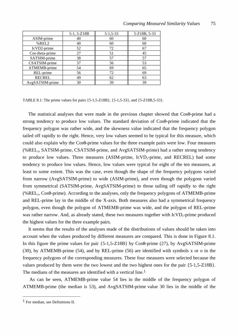
Comparing Measured Similarity Values 75
5-1, 5-Z18B 5-1,5-33 5-Z18B, 5-33 ASIM-prime 40 60 60
%REL2 40 60 60 IcVD2-prime 52 72 67
Cos-theta-prime 27 51 45 SATSIM-prime 38 57 57
CSATSIM-prime 37 56 53 ATMEMB-prime 54 69 65
REL-prime 56 72 69 RECREL 49 62 63
AvgSATSIM-prime 30 39 39
TABLE 8.1: The prime values for pairs {5-1,5-Z18B}, {5-1,5-33}, and {5-Z18B,5-33}.
The statistical analyses that were made in the previous chapter showed that Cosθ-prime had a
strong tendency to produce low values. The standard deviation of Cosθ-prime indicated that the frequency polygon was rather wide, and the skewness value indicated that the frequency polygon tailed off rapidly to the right. Hence, very low values seemed to be typical for this measure, which could also explain why the Cosθ-prime values for the three example pairs were low. Four measures (%REL2, SATSIM-prime, CSATSIM-prime, and AvgSATSIM-prime) had a rather strong tendency to produce low values. Three measures (ASIM-prime, IcVD2-prime, and RECREL) had some tendency to produce low values. Hence, low values were typical for eight of the ten measures, at least to some extent. This was the case, even though the shape of the frequency polygons varied from narrow (AvgSATSIM-prime) to wide (ASIM-prime), and even though the polygons varied from symmetrical (SATSIM-prime, AvgSATSIM-prime) to those tailing off rapidly to the right (%REL2, Cosθ-prime). According to the analyses, only the frequency polygons of ATMEMB-prime and REL-prime lay in the middle of the X-axis. Both measures also had a symmetrical frequency polygon, even though the polygon of ATMEMB-prime was wide, and the polygon of REL-prime was rather narrow. And, as already stated, these two measures together with IcVD2-prime produced the highest values for the three example pairs.
It seems that the results of the analyses made of the distributions of values should be taken into account when the values produced by different measures are compared. This is done in Figure 8.1. In this figure the prime values for pair {5-1,5-Z18B} by Cosθ-prime (27), by AvgSATSIM-prime (30), by ATMEMB-prime (54), and by REL-prime (56) are identified with symbols x or o in the frequency polygons of the corresponding measures. These four measures were selected because the values produced by them were the two lowest and the two highest ones for the pair {5-1,5-Z18B}. The medians of the measures are identified with a vertical line.1
As can be seen, ATMEMB-prime value 54 lies in the middle of the frequency polygon of ATMEMB-prime (the median is 53), and AvgSATSIM-prime value 30 lies in the middle of the
1 For median, see Definitions II.
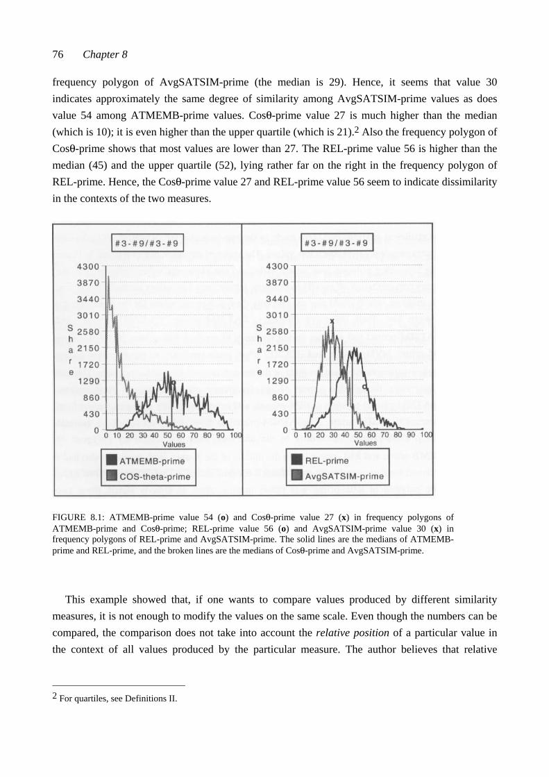
76 Chapter 8
frequency polygon of AvgSATSIM-prime (the median is 29). Hence, it seems that value 30 indicates approximately the same degree of similarity among AvgSATSIM-prime values as does value 54 among ATMEMB-prime values. Cosθ-prime value 27 is much higher than the median (which is 10); it is even higher than the upper quartile (which is 21).2 Also the frequency polygon of Cosθ-prime shows that most values are lower than 27. The REL-prime value 56 is higher than the median (45) and the upper quartile (52), lying rather far on the right in the frequency polygon of REL-prime. Hence, the Cosθ-prime value 27 and REL-prime value 56 seem to indicate dissimilarity in the contexts of the two measures.
FIGURE 8.1: ATMEMB-prime value 54 (o) and Cosθ-prime value 27 (x) in frequency polygons of ATMEMB-prime and Cosθ-prime; REL-prime value 56 (o) and AvgSATSIM-prime value 30 (x) in frequency polygons of REL-prime and AvgSATSIM-prime. The solid lines are the medians of ATMEMB-prime and REL-prime, and the broken lines are the medians of Cosθ-prime and AvgSATSIM-prime.
This example showed that, if one wants to compare values produced by different similarity
measures, it is not enough to modify the values on the same scale. Even though the numbers can be compared, the comparison does not take into account the relative position of a particular value in the context of all values produced by the particular measure. The author believes that relative
2 For quartiles, see Definitions II.
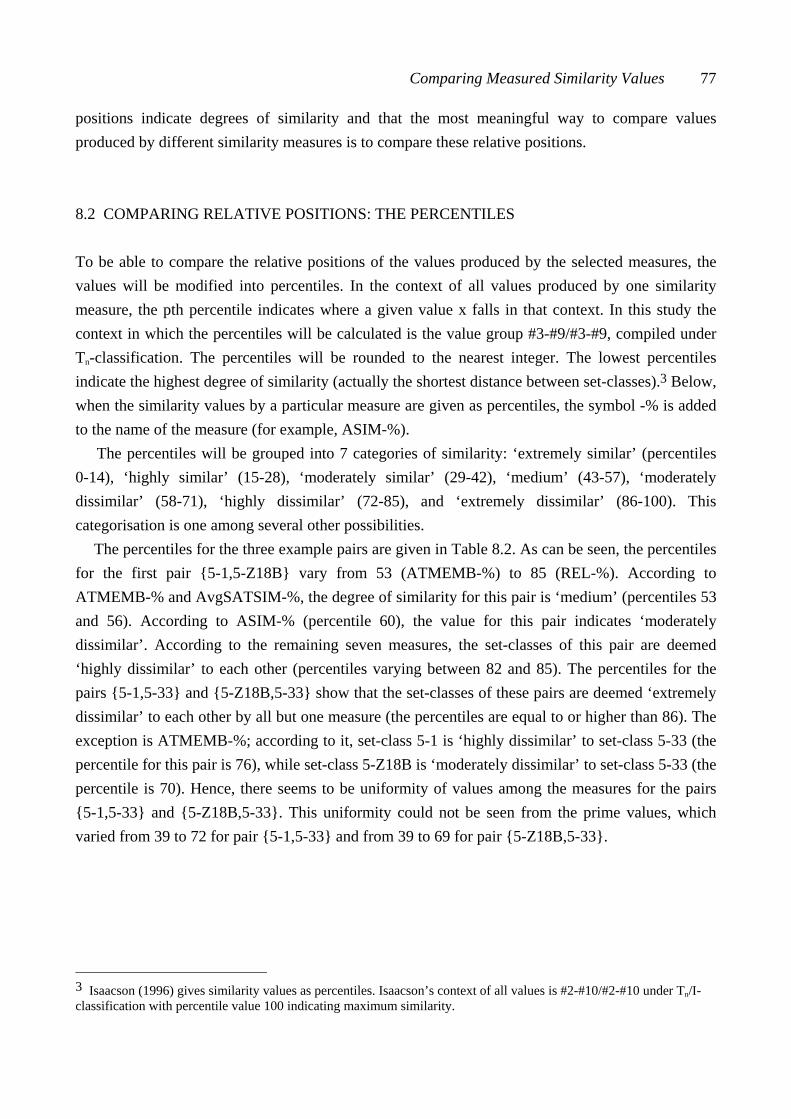
Comparing Measured Similarity Values 77
positions indicate degrees of similarity and that the most meaningful way to compare values produced by different similarity measures is to compare these relative positions.
8.2 COMPARING RELATIVE POSITIONS: THE PERCENTILES
To be able to compare the relative positions of the values produced by the selected measures, the values will be modified into percentiles. In the context of all values produced by one similarity measure, the pth percentile indicates where a given value x falls in that context. In this study the context in which the percentiles will be calculated is the value group #3-#9/#3-#9, compiled under Tn-classification. The percentiles will be rounded to the nearest integer. The lowest percentiles indicate the highest degree of similarity (actually the shortest distance between set-classes).3 Below, when the similarity values by a particular measure are given as percentiles, the symbol -% is added to the name of the measure (for example, ASIM-%).
The percentiles will be grouped into 7 categories of similarity: ‘extremely similar’ (percentiles 0-14), ‘highly similar’ (15-28), ‘moderately similar’ (29-42), ‘medium’ (43-57), ‘moderately dissimilar’ (58-71), ‘highly dissimilar’ (72-85), and ‘extremely dissimilar’ (86-100). This categorisation is one among several other possibilities.
The percentiles for the three example pairs are given in Table 8.2. As can be seen, the percentiles for the first pair {5-1,5-Z18B} vary from 53 (ATMEMB-%) to 85 (REL-%). According to ATMEMB-% and AvgSATSIM-%, the degree of similarity for this pair is ‘medium’ (percentiles 53 and 56). According to ASIM-% (percentile 60), the value for this pair indicates ‘moderately dissimilar’. According to the remaining seven measures, the set-classes of this pair are deemed ‘highly dissimilar’ to each other (percentiles varying between 82 and 85). The percentiles for the pairs {5-1,5-33} and {5-Z18B,5-33} show that the set-classes of these pairs are deemed ‘extremely dissimilar’ to each other by all but one measure (the percentiles are equal to or higher than 86). The exception is ATMEMB-%; according to it, set-class 5-1 is ‘highly dissimilar’ to set-class 5-33 (the percentile for this pair is 76), while set-class 5-Z18B is ‘moderately dissimilar’ to set-class 5-33 (the percentile is 70). Hence, there seems to be uniformity of values among the measures for the pairs {5-1,5-33} and {5-Z18B,5-33}. This uniformity could not be seen from the prime values, which varied from 39 to 72 for pair {5-1,5-33} and from 39 to 69 for pair {5-Z18B,5-33}. 3 Isaacson (1996) gives similarity values as percentiles. Isaacson’s context of all values is #2-#10/#2-#10 under Tn/I-classification with percentile value 100 indicating maximum similarity.
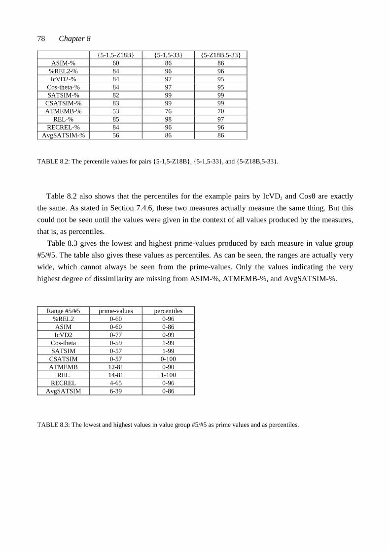
78 Chapter 8
{5-1,5-Z18B} {5-1,5-33} {5-Z18B,5-33} ASIM-% 60 86 86
%REL2-% 84 96 96 IcVD2-% 84 97 95
Cos-theta-% 84 97 95 SATSIM-% 82 99 99
CSATSIM-% 83 99 99 ATMEMB-% 53 76 70
REL-% 85 98 97 RECREL-% 84 96 96
AvgSATSIM-% 56 86 86 TABLE 8.2: The percentile values for pairs {5-1,5-Z18B}, {5-1,5-33}, and {5-Z18B,5-33}.
Table 8.2 also shows that the percentiles for the example pairs by IcVD2 and Cosθ are exactly
the same. As stated in Section 7.4.6, these two measures actually measure the same thing. But this could not be seen until the values were given in the context of all values produced by the measures, that is, as percentiles.
Table 8.3 gives the lowest and highest prime-values produced by each measure in value group #5/#5. The table also gives these values as percentiles. As can be seen, the ranges are actually very wide, which cannot always be seen from the prime-values. Only the values indicating the very highest degree of dissimilarity are missing from ASIM-%, ATMEMB-%, and AvgSATSIM-%.
Range #5/#5 prime-values percentiles
%REL2 0-60 0-96 ASIM 0-60 0-86 IcVD2 0-77 0-99
Cos-theta 0-59 1-99 SATSIM 0-57 1-99
CSATSIM 0-57 0-100 ATMEMB 12-81 0-90
REL 14-81 1-100 RECREL 4-65 0-96
AvgSATSIM 6-39 0-86 TABLE 8.3: The lowest and highest values in value group #5/#5 as prime values and as percentiles.

Comparing Measured Similarity Values 79
In the following chapters, all comparisons between values produced by different measures will be done by using percentiles.4 Terms such as ‘similarity values as percentiles’ or ‘percentiles’ will be used. The percentiles produced by the interval-class vector-based measures are given in Table A 8.1. The percentiles produced by the total measures are given in Table A 8.2. These tables are in Appendix 3.
4 The percentiles were derived through a two-step procedure. First, the measured values were modified into ‘prime’-values, that is, they were modified to lie on the scale from 0 to 100 (with 0 indicating maximum similarity), and they were rounded to integers. Second, they were modified into percentiles. It would naturally have been possible to modify the values directly into percentiles without the step into the ‘prime’-values. The ‘prime’-values were, however, important because without them it would have been difficult to compare the values and show the need of percentiles. Some of the now-obtained percentile values would probably have differed slightly if the first step with rounding had been excluded.

81
PART III TEST MATERIALS AND TESTING
The third part of the study discusses the test materials of the two empirical tests as well as the testing itself. As stated in the Introduction (Section 1.3), pentachords derived from pentad classes were used in the tests. The chords were played in pairs in the first test (the chord-pair test) and one by one in the second test (the single-chord test). Since the tests could not last too long, the number of chords and chord pairs had to be limited. Chapter 9 explains the way in which the pentad classes and pentad-class pairs were selected. Chapter 10 discusses the variables that were controlled when the pentachords and pentachord pairs were composed. The testing procedure, the subjects, and the equipment are discussed in Chapter 11.

CHAPTER NINE PENTAD CLASSES AND PENTAD-CLASS PAIRS
When the test materials were devised, pentad classes and pentad-class pairs were taken as the point of departure. Under Tn-classification the number of pentad classes is 66, and, consequently, the number of pairings in comparison group #5/#5 is 2145.1 Even if only one chord pair had represented each pentad-class pair in the chord-pair test and even if only one chord had represented each pentad class in the single-chord test, the number of test stimuli would have been too high. For this reason the number of pentad classes and pentad-class pairs to be used had to be limited.
Pentad classes, like all set-classes, can be described with the help of their properties, such as the successive-interval array, the interval-class content, and the subset-class content. The pentad classes were selected according to certain interval-class vector properties.2 These properties were the distribution of the interval-class instances in the interval-class vectors, the maximum components, and the zero components. Section 9.1 explains these properties in more detail. Section 9.2, in turn, explains how a collection of twelve pentad classes was selected according to the properties.
Three models of tonal consonance were briefly discussed in Section 5.2. Of these models, Huron’s model (1994) gives consonance indexes for interval-classes. Hence, this model can be used to calculate consonance values for set-classes. The Huron values for the selected pentad classes will be calculated in Section 9.3. The consonance values will be needed when the factors guiding the subjects’ ratings of the chord pairs are analyzed in Chapter 12.
In Section 9.4, the selected pentad classes will be paired, and similarity values as percentiles for the pairs will be calculated by the ten similarity measures that were selected in Chapter 7.3 Section 9.4 also analyzes the percentiles for the pairs.
1 For comparison group, see Definitions I. 2 For the interval-class vector, see Definitions I. 3 For percentiles, see Section 8.2.
84 Chapter 9
9.1 SOME INTERVAL-CLASS VECTOR PROPERTIES OF PENTAD CLASSES
The interval-class instances in an interval-class vector can be evenly distributed or they can be in ‘stacks’ or ‘piles’. Castrén uses the term ‘peaked interval-class distributions’ for the latter (1994a: 24). The term must be understood in the context of the particular set-class cardinality; components 3 and 4 are ‘peaks’ in interval-class vectors of pentad classes, but not in interval-class vectors of septad classes.4 Likewise, component 2 is a ‘peak’ in the interval-class vector of a triad class. Below, the term ‘peak’ is used for components 3 and 4.
The idea of maximum number of instances of each interval-class was introduced by Buchler (1998: 39). The maximum numbers are always given in the context of one particular set-class cardinality, and they are given separately for each interval-class. An example of pentad classes illuminates the idea: If one examines the interval-class vectors of all pentad classes, one can learn that the maximum number of instances of interval-class 1 to be found is four.5 A pentad class with five (or more) instances of interval-class 1 simply does not exist. The maximum number of instances of interval-class 6, in turn, is two. According to Buchler (1998: Figure 2.3), the maximum numbers of instances of interval-classes (i) of pentad classes, Max(5,i), are [444442]. In other words, there are at most four instances of interval-classes 1, 2, 3, 4, and 5 in any pentad class, and at most two instances of interval-class 6. Below, the term ‘maximum component’ is used for any interval-class vector component that is equal to the maximum.
In the context of pentad classes, the maximum component is in most cases a peak as well. The exception is maximum component 2 in index 6. However, a peak is not necessarily a maximum component. As already stated, component 3 is a peak, but 3 is never equal to the maximum.
A zero component indicates that there are no instances of the corresponding interval-class in the set-class at all. In the interval-class vector of a pentad class, a zero component is possible in every interval-class except interval-class 4. In other words, each pentad class includes at least one instance of interval-class 4.
4 The total number of interval-class instances in any pentad class is 10; if these ten interval-class instances are evenly distributed in six indexes, each component is 1 or 2. But the total number of interval-class instances in any any septad class is 21; if these are evenly distributed in six indexes, each component is 3 or 4. 5 The way in which the maximum can be derived through examining the properties of the interval cycles is discussed in Buchler (1998: 39-46).
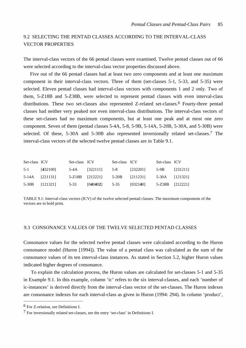
Pentad Classes and Pentad-Class Pairs 85
9.2 SELECTING THE PENTAD CLASSES ACCORDING TO THE INTERVAL-CLASS VECTOR PROPERTIES
The interval-class vectors of the 66 pentad classes were examined. Twelve pentad classes out of 66 were selected according to the interval-class vector properties discussed above.
Five out of the 66 pentad classes had at least two zero components and at least one maximum component in their interval-class vectors. Three of them (set-classes 5-1, 5-33, and 5-35) were selected. Eleven pentad classes had interval-class vectors with components 1 and 2 only. Two of them, 5-Z18B and 5-Z38B, were selected to represent pentad classes with even interval-class distributions. These two set-classes also represented Z-related set-classes.6 Fourty-three pentad classes had neither very peaked nor even interval-class distributions. The interval-class vectors of these set-classes had no maximum components, but at least one peak and at most one zero component. Seven of them (pentad classes 5-4A, 5-8, 5-9B, 5-14A, 5-20B, 5-30A, and 5-30B) were selected. Of these, 5-30A and 5-30B also represented inversionally related set-classes.7 The interval-class vectors of the selected twelve pentad classes are in Table 9.1.
Set-class ICV Set-class ICV Set-class ICV Set-class ICV
5-1 [432100] 5-4A [322111] 5-8 [232201] 5-9B [231211]
5-14A [221131] 5-Z18B [212221] 5-20B [211231] 5-30A [121321]
5-30B [121321] 5-33 [040402] 5-35 [032140] 5-Z38B [212221] TABLE 9.1: Interval-class vectors (ICV) of the twelve selected pentad classes. The maximum components of the vectors are in bold print.
9.3 CONSONANCE VALUES OF THE TWELVE SELECTED PENTAD CLASSES
Consonance values for the selected twelve pentad classes were calculated according to the Huron consonance model (Huron [1994]). The value of a pentad class was calculated as the sum of the consonance values of its ten interval-class instances. As stated in Section 5.2, higher Huron values indicated higher degrees of consonance.
To explain the calculation process, the Huron values are calculated for set-classes 5-1 and 5-35 in Example 9.1. In this example, column ‘ic’ refers to the six interval-classes, and each ‘number of ic-instances’ is derived directly from the interval-class vector of the set-classes. The Huron indexes are consonance indexes for each interval-class as given in Huron (1994: 294). In column ‘product’, 6 For Z-relation, see Definitions I. 7 For inversionally related set-classes, see the entry ‘set-class’ in Definitions I.
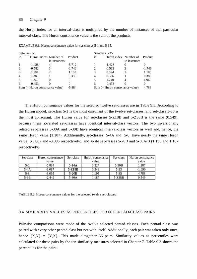
86 Chapter 9
the Huron index for an interval-class is multiplied by the number of instances of that particular interval-class. The Huron consonance value is the sum of the products.
EXAMPLE 9.1: Huron consonance value for set-classes 5-1 and 5-35. Set-class 5-1 Set-class 5-35 ic Huron index Number of Product ic Huron index Number of Product ic-instances ic-instances 1 -1.428 4 -5.712 1 -1.428 0 0 2 -0.582 3 -1.746 2 -0.582 3 -1.746 3 0.594 2 1.188 3 0.594 2 1.188 4 0.386 1 0.386 4 0.386 1 0.386 5 1.240 0 0 5 1.240 4 4.960 6 -0.453 0 0 6 -0.453 0 0 Sum (= Huron consonance value) -5.884 Sum (= Huron consonance value) 4.788
The Huron consonance values for the selected twelve set-classes are in Table 9.5. According to
the Huron model, set-class 5-1 is the most dissonant of the twelve set-classes, and set-class 5-35 is the most consonant. The Huron value for set-classes 5-Z18B and 5-Z38B is the same (0.549), because these Z-related set-classes have identical interval-class vectors. The two inversionally related set-classes 5-30A and 5-30B have identical interval-class vectors as well and, hence, the same Huron value (1.187). Additionally, set-classes 5-4A and 5-8 have nearly the same Huron value (-3.087 and -3.095 respectively), and so do set-classes 5-20B and 5-30A/B (1.195 and 1.187 respectively).
Set-class Huron consonance
value Set-class Huron consonance
value Set-class Huron consonance
value 5-1 -5.884 5-14A 0.227 5-30B 1.187
5-4A -3.087 5-Z18B 0.549 5-33 -1.690 5-8 -3.095 5-20B 1.195 5-35 4.788
5-9B -2.449 5-30A 1.187 5-Z38B 0.549 TABLE 9.2: Huron consonance values for the selected twelve set-classes.
9.4 SIMILARITY VALUES AS PERCENTILES FOR 66 PENTAD-CLASS PAIRS
Pairwise comparisons were made of the twelve selected pentad classes. Each pentad class was paired with every other pentad class but not with itself. Additionally, each pair was taken only once, hence {X,Y} = {Y,X}. This made altogether 66 pairs. Similarity values as percentiles were calculated for these pairs by the ten similarity measures selected in Chapter 7. Table 9.3 shows the percentiles for the pairs.
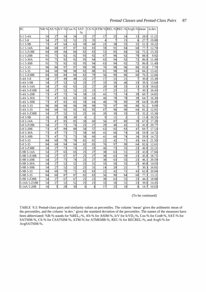
Pentad Classes and Pentad-Class Pairs 87
SC %R-% AS-% IcV-% Cos-% SAT-%
CS-% ATM-% REL-% REC-% AvgS-% mean st.dev.
5-1 5-4A 54 27 34 34 25 27 17 25 24 13 28.0 11.215-1 5-8 54 27 52 52 25 35 4 7 15 6 27.7 19.885-1 5-9B 73 47 64 63 58 60 22 38 55 31 51.5 16.225-1 5-14A 84 60 87 87 82 83 59 91 84 60 77.7 12.705-1 5-Z18B 84 60 84 84 82 83 53 85 84 56 75.5 13.355-1 5-20B 91 75 92 92 95 92 67 96 92 78 88.0 9.925-1 5-30A 91 75 92 92 95 94 63 94 92 72 86.0 11.495-1 5-30B 91 75 92 92 95 94 63 94 92 72 86.0 11.495-1 5-33 96 86 97 97 99 99 76 98 96 86 93.0 7.705-1 5-35 84 60 98 98 82 88 81 98 89 64 84.2 13.415-1 5-Z38B 84 60 84 84 82 79 56 90 86 60 76.5 12.665-4A 5-8 54 27 49 48 25 27 17 25 21 7 30.0 15.305-4A 5-9B 54 27 52 52 25 27 33 56 46 23 39.5 13.645-4A 5-14A 54 27 65 65 25 27 20 30 33 13 35.9 18.625-4A 5-Z18B 54 27 52 52 25 23 17 25 21 7 30.3 16.435-4A 5-20B 73 47 75 74 58 53 41 73 74 39 60.7 14.815-4A 5-30A 73 47 82 82 58 64 46 78 78 39 64.7 16.305-4A 5-30B 73 47 82 82 58 64 46 78 80 39 64.9 16.495-4A 5-33 96 86 96 96 99 99 70 97 96 86 92.1 9.095-4A 5-35 84 60 92 92 82 85 67 96 90 64 81.2 12.915-4A 5-Z38B 54 27 52 52 25 16 20 30 33 13 32.2 15.365-8 5-9B 16 5 28 30 6 2 9 11 2 1 11.0 10.555-8 5-14A 73 47 85 85 58 60 56 87 80 39 67.0 17.285-8 5-Z18B 54 27 73 74 25 27 29 46 42 13 41.0 20.775-8 5-20B 73 47 89 88 58 57 63 92 83 47 69.7 17.535-8 5-30A 73 47 73 73 58 60 41 66 74 34 59.9 14.725-8 5-30B 73 47 73 73 58 60 41 66 74 34 59.9 14.725-8 5-33 84 60 78 78 82 81 22 42 71 43 64.1 21.505-8 5-35 84 60 94 94 82 85 76 97 90 64 82.6 12.615-8 5-Z38B 54 27 73 74 25 19 46 73 55 23 46.9 22.215-9B 5-14A 54 27 65 65 25 27 38 63 51 23 43.8 17.665-9B 5-Z18B 54 27 67 67 25 27 38 63 59 23 45.0 18.715-9B 5-20B 54 27 75 74 25 27 38 63 55 23 46.1 20.595-9B 5-30A 54 27 52 52 25 31 33 56 55 23 40.8 14.035-9B 5-30B 54 27 52 52 25 31 14 20 21 7 30.3 16.815-9B 5-33 84 60 70 71 82 83 22 42 71 43 62.8 20.845-9B 5-35 84 60 87 87 82 83 56 90 84 60 77.3 13.115-9B 5-Z38B 54 27 67 67 25 23 38 63 55 23 44.2 18.885-14A 5-Z18B 54 27 52 52 25 23 33 56 51 23 39.6 14.455-14A 5-20B 16 5 28 30 6 4 17 25 10 6 14.7 10.03 (To be continued) TABLE 9.3: Pentad-class pairs and similarity values as percentiles. The column ‘mean’ gives the arithmetic mean of the percentiles, and the column ‘st.dev.’ gives the standard deviation of the percentiles. The names of the measures have been abbreviated: %R-% stands for %REL2-%, AS-% for ASIM-%, IcV for IcVD2-%, Cos-% for Cosθ-%, SAT-% for SATSIM-%, CS-% for CSATSIM-%, ATM-% for ATMEMB-%, REC-% for RECREL-%, and AvgS-% for AvgSATSIM-%.

88 Chapter 9
SC %R-% AS-% IcV-% Cos-% SAT-%
CS-% ATM-% REL-% REC-% AvgS-% mean st.dev.
5-14A 5-30A 54 27 65 65 25 31 20 30 38 13 36.8 18.415-14A 5-30B 54 27 65 65 25 31 20 30 42 13 37.2 18.495-14A 5-33 96 86 96 96 99 99 70 97 96 86 92.1 9.095-14A 5-35 73 47 64 63 58 53 25 42 59 31 51.5 15.225-14A 5-Z38B 54 27 52 52 25 23 38 59 51 23 40.4 14.685-Z18B 5-20B 16 5 30 30 6 2 14 20 6 3 13.2 10.645-Z18B 5-30A 54 27 52 52 25 27 17 25 24 7 31.0 16.115-Z18B 5-30B 54 27 52 52 25 27 38 59 55 23 41.2 14.575-Z18B 5-33 96 86 95 95 99 99 70 97 96 86 91.9 9.005-Z18B 5-35 84 60 84 84 82 79 56 90 86 60 76.5 12.665-Z18B 5-Z38B 0 0 0 1 1 0 11 14 1 1 2.9 5.135-20B 5-30A 54 27 52 52 25 23 29 46 38 16 36.2 13.985-20B 5-30B 54 27 52 52 25 23 20 30 29 13 32.5 14.745-20B 5-33 96 86 96 96 99 98 70 97 96 86 92.0 9.015-20B 5-35 84 60 78 78 82 79 49 83 78 51 72.2 13.485-20B 5-Z38B 16 5 30 30 6 4 20 27 15 6 15.9 10.515-30A 5-30B 0 0 0 1 1 0 22 30 2 2 5.8 10.845-30A 5-33 84 60 70 71 82 79 20 38 71 43 61.8 21.355-30A 5-35 84 60 78 78 82 81 25 49 76 43 65.6 20.355-30A 5-Z38B 54 27 52 52 25 31 29 46 46 16 37.8 13.665-30B 5-33 84 60 70 71 82 79 20 38 71 43 61.8 21.355-30B 5-35 84 60 78 78 82 81 25 49 76 43 65.6 20.355-30B 5-Z38B 54 27 52 52 25 31 38 59 59 23 42.0 14.665-33 5-35 96 86 97 97 99 99 76 98 96 86 93.0 7.705-33 5-Z38B 96 86 95 95 99 99 70 97 96 86 91.9 9.005-35 5-Z38B 84 60 84 84 82 83 53 85 84 51 75.0 14.23 TABLE 9.3 (cont.)
A first glance at Table 9.3 shows that there are seven distinct percentile values in the columns %REL2-%, ASIM-%, and SATSIM-%. As stated in Chapter 7, these three measures produce only seven distinct values in value group #5/#5. Hence, cases representing each category are included in the 66 selected pentad-class pairs. Table 9.3 shows also cases in which there is much variation in the percentiles for a pair (see, for example, the pair {5-1,5-8}), and cases in which there is only very little variation (for example, the pair {5-Z18B,5-Z38B}). To examine this variation in more detail, the standard deviation of the ten percentiles for each pair was calculated.8 Applied to the ten percentiles for each pair, the standard deviation described the variation of the percentiles among the measures: the lower the standard deviation, the smaller the variation. The standard deviations are given in the last column (‘st.dev.’) in Table 9.3.
The lowest standard deviation of the percentiles was 5.13 for the above mentioned set-class pair {5-Z18B,5-Z38B}. The next-to-lowest standard deviations were 7.70 for pairs {5-1,5-33} and {5-33,5-35}, 9.00 for pairs {5-Z18B,5-33} and {5-33,5-Z38B}, 9.01 for pair {5-20B,5-33}, and 9.09 for pairs {5-4A,5-33} and {5-14A,5-33}. All these standard deviations could be said to indicate little variation and, hence, uniformity of percentiles among the ten similarity measures.
8 For standard deviation, see Definitions II.
Pentad Classes and Pentad-Class Pairs 89
As can be seen from the percentiles in Table 9.3, all measures deemed the set-classes of pair {5-Z18B,5-Z38B} ‘extremely similar’ to each other, since the percentiles were between 0 and 14.9 This could naturally be seen from the arithmetic mean of the percentiles as well (the arithmetic mean was 2.9; see column ‘mean’ in Table 9.3). Furthermore, all measures except ATMEMB-% deemed the set-classes of the latter seven set-class pairs ‘extremely dissimilar’ to each other (the percentiles by ATMEMB-% were 70 or 76, and the percentiles by the other measures varied from 86 to 99). Consequently, the arithmetic means for these pairs were high (between 91.9 and 93.0).
The highest standard deviation of the ten percentiles was 22.21 for set-class pair {5-8,5-Z38B}. This value indicated the widest variation among the ten measures within these data. The next-to-highest standard deviations were 21.50 for pair {5-8,5-33}, 21.35 for pairs {5-30A,5-33} and {5-30B,5-33}, 20.84 for pair {5-9B,5-33}, 20.77 for pair {5-8,5-Z18B}, 20.59 for pair {5-9B,5-20B}, and 20.35 for pairs {5-30A,5-35} and {5-30B,5-35}. All these standard deviation values could be said to indicate wide variation and, hence, dispersion among the similarity measures.
If there was dispersion among the measures, the arithmetic mean of the percentiles was neither high nor low, but rather near medium. For the nine pairs discussed above, the arithmetic mean of percentiles varied from 41.0 (‘moderately similar’) for the pair {5-8,5-Z18B} to 65.6 (‘moderately dissimilar’) for pairs {5-30A,5-35} and {5-30B,5-35}. As also can be seen, there were no cases with very little variation of percentiles (and, hence, low standard deviation) and with the arithmetic mean near medium in these data. Yet it is unclear whether this was owing to the data of selected pentad-class pairs, or whether the properties of the measures were the reason for this finding.
As can be seen from Table 9.3, the percentiles for the set-class pairs by the two measures using geometric formulae (IcVD2-% and Cosθ-%) were the same for most pairs.10 And, as stated in Section 8.2, these similarity measures actually measure the same thing. Hence, below, Cosθ-% will represent both of these measures. Table 9.3 also shows that the percentiles produced by the interval-class saturation-based measures (SATSIM-% and CSATSIM-%) were very close to each other. This indicated that the differences between interval-class saturation (SATSIM-%) and interval-class cycle saturation (CSATSIM-%) were extremely small, at least within this sample of pentad classes.
9 The seven categories of similarity were defined in Section 8.2. 10 It is most likely that the small differences in the percentile values were caused by the fact that the prime-values were rounded to the nearest integer.
CHAPTER TEN CHORDS AND CHORD PAIRS
This chapter discusses the pentachords and pentachord pairs that were used as test materials in the two empirical tests. These chords were composed from the twelve set-classes that were selected in Chapter 9.
One set-class can be represented by an infinite number of chords, and it is impossible to define an ‘ideal representative’ of the set-class. All chords derived from a set-class reflect its structural properties (for example, the total interval-class and the total subset-class content), even though the chordal characteristics (for example, pitch content, interval content, width, register, overall shape, etc.) of the chords can differ greatly. Section 10.1 discusses the variables of chordal setting that were controlled when the chord pairs were composed. By controlling these variables the number of possible pairs was restricted. The test chords are presented in this section in Example 10.1.
Three models of tonal consonance were discussed in Section 5.2. Of these models, the model by Malmberg (1918) and the model by Kameoka and Kuriyagawa (1969) can be used to calculate consonance values for chords. The consonance values will be calculated for the selected pentachords by these models in Section 10.2. These values will be needed, when the factors guiding the subjects’ ratings of the chords are analyzed in Chapter 13.
10.1 COMPOSING THE CHORD PAIRS REPRESENTING THE SET-CLASS PAIRS
Sixty-six chord pairs were composed in order to represent the 66 set-class pairs formed from the twelve pentad classes selected in the previous chapter. The first variable that was controlled when the chord pairs were composed was the width of the chords. Two widths, 15 and 16 semitones, were selected. It seemed that pentachords with these widths were neither very close-spaced, nor very open-spaced. The width of 15 semitones gave the chords the outer interval of a minor tenth, while the width of 16 semitones gave the chords that of a major tenth.
Chords and Chord Pairs 91
It was possible to compose 16 semitone chords from each of the twelve pentad classes. This was the case because, as stated in Section 9.1, each pentad class has at least one instance of interval-class 4 (the interval 16 belongs to interval-class 4). The width of 15 semitones was impossible only for chords derived from set-class 5-33.
The second variable was the number of common pitch-classes between the two chords of one pair. There were different possibilities from no common pitch-classes to the maximum possible number of common pitch-classes. The maximum number was chosen to be used. The maximum was defined as the number of elements in the largest mutually embeddable subset-class of the two set-classes from which the chords were derived. Within the sample of these twelve set-classes and 66 pairs derived from them, this number was either three or four. This meant that all pairs of the chord-pair test fell in only two different categories; those with three pitch-classes in common and those with four pitch-classes in common.
The third variable was the registral placement of the pitches representing the common pitch-classes. All common pitch-classes were represented by common pitches.1 Additionally, two of the common pitches were placed in the outer voices of the chords of each pair, which indicated that both chords in a pair had the same width. The outer pitches of the chords were kept constant, even though the non-common pitches would probably have been easier to notice if they had been in the outer voices of the chords.2 But if these pitches had been in the outer voices, the changes in outer voices would have drawn the subjects’ attention to them. It was likely that the changes in outer voices would have dominated perception. Additionally, it was likely that the difference between the two categories (a change in one outer voice or changes in both outer voices) would have affected the perception of closeness rather strongly (perhaps even crucially). It also seemed easier to avoid associations with harmonic progressions or melodic sequences between chords when the outer voices did not move.
The fourth variable that was controlled when the chord pairs were composed was the number of chords representing each set-class. The ideal was that only two chords, one of width 15 and one of width 16 semitones, would have represented each set-class. The reason for this is as follows: The chord-pair test was made to collect closeness ratings that could be compared with similarity values produced by different measures. For this comparison, the set-classes could have been represented by an unlimited number of chords. But the chord-pair dataset is also analyzed by the multidimensional scaling method.3 The problem of using this method for analyzing the chord-pair
1 This decision was based on the finding in Gibson (1993) that the shared pitch content, but not the shared pitch-class content, is in connection with subjects’ similarity ratings (see Section 3.2.1). See also the criticism of the earlier studies in Chapter 4. 2 In a study concerning the perceptibility of concurrent voices, Huron observed that entries of inner voices were significantly more difficult to identify than entries of outer voices (Huron [1989: 369]). 3 For multidimensional scaling, see Definitions III.
92 Chapter 10
dataset is that all chords deriving from one set-class are processed as one object. For this reason the number of chords representing each set-class had to be as few as possible.4
Finally, the twelve set-classes were represented by 28 chords, two chords from set-classes 5-1, 5-8, 5-9B, 5-14A, 5-20B, 5-30A, 5-33, and 5-35 and three chords from set-classes 5-4A, 5-Z18B, 5-30B, and 5-Z38B. Hence, the ideal of two chords derived from each set-class was not achieved.5 And, as already stated, from set-class 5-33 it was possible to make chords with the width of 16 semitones only. The number of 16 semitone chords was 16, and the number of 15 semitone chords was 12.
The fifth variable was the register. Middle register was chosen to be used. The lowest pitch of each chord was set between A3 and C#4, hence, the register used in the tests was between A3 and F5. These rather small changes in transpositional levels were made in order to avoid the same outer pitches in chords in adjacent items.6
The 28 test chords are in Example 10.1. In this example the chords are given on the same transpositional level as they were played to the subjects in the single-chord test. As can be seen from the example, the lowest pitch was A3 in six chords, Bb3 in six chords, B3 in five chords, C4 in seven chords, and C#4 in four chords.
The same 28 chords were used when the 66 chord pairs were made to represent the 66 set-class pairs. The integer in parentheses in Example 10.1 indicates how many times each chord was used in the 66 pairs. As can be seen, chords 4, 14, 19, and 26 (derived from set-classes 5-4A, 5-Z18B, 5-30B, and 5-Z38B, respectively) were used in only one pair. Hence, the 66 pairs were mainly formed of 24 chords. The number of pairs with 16 semitone chords was 39, and the number of pairs with 15 semitone chords was 27. The lowest pitch was A3 in 11 pairs, Bb3 in 13 pairs, B3 in 14 pairs, C4 in 14 pairs, and C#4 in 14 pairs. The number of pairs with four common pitches was 26, and the number of pairs with three common pitches was 40. The 66 chord pairs are in Appendix 4.7
4 The other possibility would have been to use the chords, not set-classes, as objects in the multidimensional scaling analysis. This would also have created problems: every chord would have to be paired with every other chord, which would not have been possible under the testing regime discussed above. 5 It is possible that a solution with only two chords from each set-class would have been found if the work had been done with the help of a computer. 6 Four of the variables of chordal setting controlled in this study (the two chords had the same width, the same outer pitches, the maximum number of common pitches, and were played in the middle register) were identical to those used in Castrén (2000). 7 The whole chord-pair test had 75 pairs; the 66 pairs derived from the 66 set-class pairs and nine additional pairs; see Chapter 12.
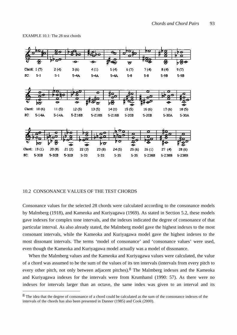
Chords and Chord Pairs 93
EXAMPLE 10.1: The 28 test chords
10.2 CONSONANCE VALUES OF THE TEST CHORDS Consonance values for the selected 28 chords were calculated according to the consonance models by Malmberg (1918), and Kameoka and Kuriyagawa (1969). As stated in Section 5.2, these models gave indexes for complex tone intervals, and the indexes indicated the degree of consonance of that particular interval. As also already stated, the Malmberg model gave the highest indexes to the most consonant intervals, while the Kameoka and Kuriyagawa model gave the highest indexes to the most dissonant intervals. The terms ‘model of consonance’ and ‘consonance values’ were used, even though the Kameoka and Kuriyagawa model actually was a model of dissonance.
When the Malmberg values and the Kameoka and Kuriyagawa values were calculated, the value of a chord was assumed to be the sum of the values of its ten intervals (intervals from every pitch to every other pitch, not only between adjacent pitches).8 The Malmberg indexes and the Kameoka and Kuriyagawa indexes for the intervals were from Krumhansl (1990: 57). As there were no indexes for intervals larger than an octave, the same index was given to an interval and its 8 The idea that the degree of consonance of a chord could be calculated as the sum of the consonance indexes of the intervals of the chords has also been presented in Danner (1985) and Cook (2000).
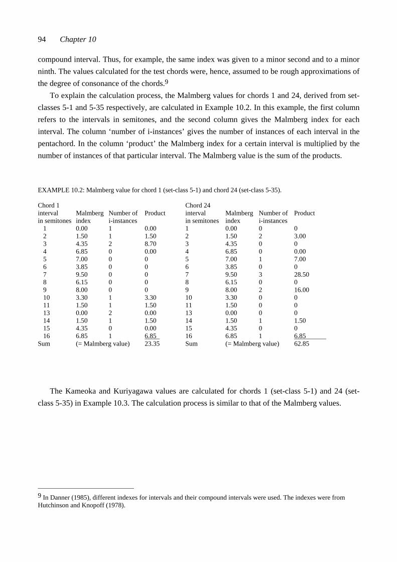
94 Chapter 10
compound interval. Thus, for example, the same index was given to a minor second and to a minor ninth. The values calculated for the test chords were, hence, assumed to be rough approximations of the degree of consonance of the chords.9
To explain the calculation process, the Malmberg values for chords 1 and 24, derived from set-classes 5-1 and 5-35 respectively, are calculated in Example 10.2. In this example, the first column refers to the intervals in semitones, and the second column gives the Malmberg index for each interval. The column ‘number of i-instances’ gives the number of instances of each interval in the pentachord. In the column ‘product’ the Malmberg index for a certain interval is multiplied by the number of instances of that particular interval. The Malmberg value is the sum of the products.
EXAMPLE 10.2: Malmberg value for chord 1 (set-class 5-1) and chord 24 (set-class 5-35).
Chord 1 Chord 24 interval Malmberg Number of Product interval Malmberg Number of Product in semitones index i-instances in semitones index i-instances
1 0.00 1 0.00 1 0.00 0 0 2 1.50 1 1.50 2 1.50 2 3.00 3 4.35 2 8.70 3 4.35 0 0 4 6.85 0 0.00 4 6.85 0 0.00 5 7.00 0 0 5 7.00 1 7.00 6 3.85 0 0 6 3.85 0 0 7 9.50 0 0 7 9.50 3 28.50 8 6.15 0 0 8 6.15 0 0 9 8.00 0 0 9 8.00 2 16.00 10 3.30 1 3.30 10 3.30 0 0 11 1.50 1 1.50 11 1.50 0 0 13 0.00 2 0.00 13 0.00 0 0 14 1.50 1 1.50 14 1.50 1 1.50 15 4.35 0 0.00 15 4.35 0 0 16 6.85 1 6.85 16 6.85 1 6.85
Sum (= Malmberg value) 23.35 Sum (= Malmberg value) 62.85
The Kameoka and Kuriyagawa values are calculated for chords 1 (set-class 5-1) and 24 (set-
class 5-35) in Example 10.3. The calculation process is similar to that of the Malmberg values.
9 In Danner (1985), different indexes for intervals and their compound intervals were used. The indexes were from Hutchinson and Knopoff (1978).
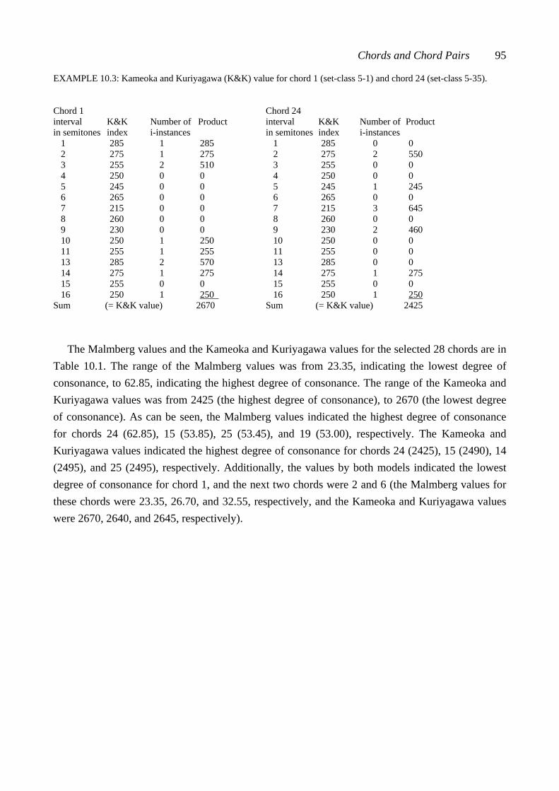
Chords and Chord Pairs 95
EXAMPLE 10.3: Kameoka and Kuriyagawa (K&K) value for chord 1 (set-class 5-1) and chord 24 (set-class 5-35).
Chord 1 Chord 24 interval K&K Number of Product interval K&K Number of Product in semitones index i-instances in semitones index i-instances
1 285 1 285 1 285 0 0 2 275 1 275 2 275 2 550 3 255 2 510 3 255 0 0 4 250 0 0 4 250 0 0 5 245 0 0 5 245 1 245 6 265 0 0 6 265 0 0 7 215 0 0 7 215 3 645 8 260 0 0 8 260 0 0 9 230 0 0 9 230 2 460 10 250 1 250 10 250 0 0 11 255 1 255 11 255 0 0 13 285 2 570 13 285 0 0 14 275 1 275 14 275 1 275 15 255 0 0 15 255 0 0 16 250 1 250 16 250 1 250
Sum (= K&K value) 2670 Sum (= K&K value) 2425
The Malmberg values and the Kameoka and Kuriyagawa values for the selected 28 chords are in
Table 10.1. The range of the Malmberg values was from 23.35, indicating the lowest degree of consonance, to 62.85, indicating the highest degree of consonance. The range of the Kameoka and Kuriyagawa values was from 2425 (the highest degree of consonance), to 2670 (the lowest degree of consonance). As can be seen, the Malmberg values indicated the highest degree of consonance for chords 24 (62.85), 15 (53.85), 25 (53.45), and 19 (53.00), respectively. The Kameoka and Kuriyagawa values indicated the highest degree of consonance for chords 24 (2425), 15 (2490), 14 (2495), and 25 (2495), respectively. Additionally, the values by both models indicated the lowest degree of consonance for chord 1, and the next two chords were 2 and 6 (the Malmberg values for these chords were 23.35, 26.70, and 32.55, respectively, and the Kameoka and Kuriyagawa values were 2670, 2640, and 2645, respectively).
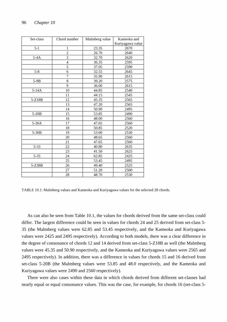
96 Chapter 10
Set-class Chord number Malmberg value Kameoka and
Kuriyagawa value5-1 1 23.35 2670
2 26.70 2640 5-4A 3 32.70 2620
4 36.35 2595 5 37.05 2590
5-8 6 32.55 2645 7 35.90 2615
5-9B 8 39.20 2575 9 36.00 2615
5-14A 10 44.85 2540 11 44.15 2545
5-Z18B 12 45.35 2565 13 47.20 2565 14 50.90 2495
5-20B 15 53.85 2490 16 48.00 2560
5-30A 17 47.65 2560 18 50.85 2520
5-30B 19 53.00 2530 20 48.65 2560 21 47.65 2560
5-33 22 40.80 2635 23 41.50 2625
5-35 24 62.85 2425 25 53.45 2495
5-Z38B 26 49.40 2525 27 51.20 2500 28 48.70 2530
TABLE 10.1: Malmberg values and Kameoka and Kuriyagawa values for the selected 28 chords.
As can also be seen from Table 10.1, the values for chords derived from the same set-class could
differ. The largest difference could be seen in values for chords 24 and 25 derived from set-class 5-35 (the Malmberg values were 62.85 and 53.45 respectively, and the Kameoka and Kuriyagawa values were 2425 and 2495 respectively). According to both models, there was a clear difference in the degree of consonance of chords 12 and 14 derived from set-class 5-Z18B as well (the Malmberg values were 45.35 and 50.90 respectively, and the Kameoka and Kuriyagawa values were 2565 and 2495 respectively). In addition, there was a difference in values for chords 15 and 16 derived from set-class 5-20B (the Malmberg values were 53.85 and 48.0 respectively, and the Kameoka and Kuriyagawa values were 2490 and 2560 respectively).
There were also cases within these data in which chords derived from different set-classes had nearly equal or equal consonance values. This was the case, for example, for chords 16 (set-class 5-
Chords and Chord Pairs 97
20B), 17 (5-30A), 20, and 21 (5-30B). These chords had Malmberg values 48.0, 47.65, 48.65, and 47.65, respectively, and they all had the same Kameoka and Kuriyagawa value 2560.
The correlation between the Malmberg values and the Kameoka and Kuriyagawa values for the 28 chords was -0.93. This correlation was very high and statistically very significant, indicating that, at least within this sample of pentachords, there was uniformity of consonance values produced by these models. This was the case even though the indexes for intervals were based on rather dissimilar aspects in these models (as stated in Section 5.2, Malmberg’s model was based on empirical recordings from musically experienced subjects, while Kameoka and Kuriyagawa’s model was based on theoretical calculations tested with inexperienced subjects). The correlation was negative since the Malmberg model gave the highest values for the most consonant chords and the Kameoka and Kuriyagawa model gave the highest values for the most dissonant chords.
CHAPTER ELEVEN THE TESTS This chapter describes the testing procedure. The two empirical tests are explained in Section 11.1. Section 11.2 discusses the technical procedure of recording the test items. The length and order of the test items in the chord-pair test and in the single-chord test are described in Section 11.3. The backgrounds of the subjects, according to the questionnaire in the test form, are analyzed in Section 11.4. Section 11.5 explains the scoring of the responses given by the subjects.
11.1 THE TWO TESTS
In the chord-pair test, the subjects were asked to rate how close or distant the two chords in each pair were. What was meant by closeness between two chords was not defined; thus, the subjects were allowed to define for themselves the basis for their ratings. The subjects were asked to make their ratings rather quickly, on the basis of their initial intuition. They were also encouraged to pay attention to the general quality, that is, to some kind of overall impression of the chords, in preference to analyzing the individual pitches of the chords. Additionally, they were told that the test was made to collect their opinions, and it was emphasised that there were no right answers.
The closeness ratings were made on a seven-step rating scale. The scale was bipolar. The word at the left end of the scale indicated ‘close’ or ‘near’, and the word at the right end of the scale indicated ‘distant’, ‘remote’, or ‘far’. These words (‘läheinen’ and ‘etäinen’ respectively) were naturally in Finnish. There were three values for both words on the scale. Additionally, value 0 in the middle of the scale indicated neither distance nor closeness (the scale is in Example 11.1; the whole test form is in Appendix 1). This kind of a rating scale was selected, because the author assumed that the subjects could easily associate the value 0 with the middle point of the scale. Further, there were the same three numbers on both sides of the scale; hence neither of the characteristics at the ends of the scale was ‘higher’ or ‘lower’ (or ‘better’ or ‘worse’) than the other.
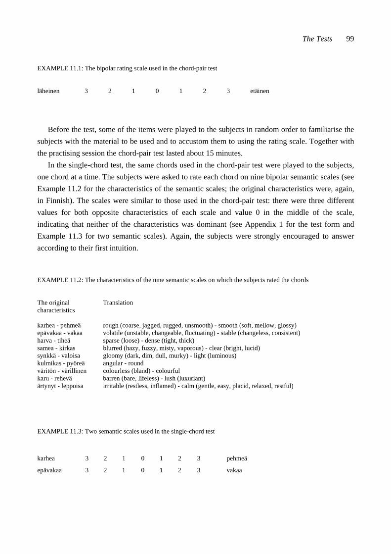
The Tests 99
EXAMPLE 11.1: The bipolar rating scale used in the chord-pair test läheinen 3 2 1 0 1 2 3 etäinen
Before the test, some of the items were played to the subjects in random order to familiarise the
subjects with the material to be used and to accustom them to using the rating scale. Together with the practising session the chord-pair test lasted about 15 minutes.
In the single-chord test, the same chords used in the chord-pair test were played to the subjects, one chord at a time. The subjects were asked to rate each chord on nine bipolar semantic scales (see Example 11.2 for the characteristics of the semantic scales; the original characteristics were, again, in Finnish). The scales were similar to those used in the chord-pair test: there were three different values for both opposite characteristics of each scale and value 0 in the middle of the scale, indicating that neither of the characteristics was dominant (see Appendix 1 for the test form and Example 11.3 for two semantic scales). Again, the subjects were strongly encouraged to answer according to their first intuition.
EXAMPLE 11.2: The characteristics of the nine semantic scales on which the subjects rated the chords
The original Translation characteristics karhea - pehmeä rough (coarse, jagged, rugged, unsmooth) - smooth (soft, mellow, glossy) epävakaa - vakaa volatile (unstable, changeable, fluctuating) - stable (changeless, consistent) harva - tiheä sparse (loose) - dense (tight, thick) samea - kirkas blurred (hazy, fuzzy, misty, vaporous) - clear (bright, lucid) synkkä - valoisa gloomy (dark, dim, dull, murky) - light (luminous) kulmikas - pyöreä angular - round väritön - värillinen colourless (bland) - colourful karu - rehevä barren (bare, lifeless) - lush (luxuriant) ärtynyt - leppoisa irritable (restless, inflamed) - calm (gentle, easy, placid, relaxed, restful) EXAMPLE 11.3: Two semantic scales used in the single-chord test
karhea 3 2 1 0 1 2 3 pehmeä
epävakaa 3 2 1 0 1 2 3 vakaa
100 Chapter 11
The single-chord test took about 20 minutes. There was a short pause between the two tests, during which the subjects answered a questionnaire. The questions concerned the age, sex, studies, and listening habits of the subjects (these will be discussed in Section 11.4).
The idea of the bipolar scales used in the single-chord test came from the semantic differential (Osgood, Suci, and Tannenbaum [1957]). Only nine scales were used in the present test, even though the tests applying semantic differential usually use up to 50 scales. The author believed that the subjects would be able to concentrate better if the two tests together with the break between them lasted no longer than about 45 minutes. The characteristics of the nine scales were selected so that they had relevance to the chords being judged (for example, scales like ‘grateful-ungrateful’, ‘true-false’ or ‘fast-slow’ would not have had such relevance). The selected characteristics were, however, not fixed in Western music theory to indicate something definite (such as ‘major-minor’). Nor were they words that are commonly used when music is described (such as ‘consonant-dissonant’). Additionally, the characteristics selected were of different types and they were very common.
11.2 THE EQUIPMENT AND THE SOUND SAMPLE
The chords were first played on a Yamaha KX 88 keyboard. The midi information thus obtained was sent to a Logic Audio program running on a Power Macintosh 9600/300 computer by means of the Midi Time Peace II midi interface. On the Logic Audio program the pitches of each chord were given equal length by quantifying the note values. Hence, the pitches started and stopped in perfect simultaneity. In addition, the velocity was set the same for each key in order to assure the same objective dynamic level for each pitch.
A grand piano sound from the Samplecell II CD-Rom library was used when the chord sounds were played. The piano sound was chosen because it was familiar to the subjects and because it is possible to play block-chords on the piano. Circular tones (also called ‘Shepard’ tones) are often used in this kind of study to eliminate the effects of register and voice leading and to minimise the sense of chord progression. However, circular tones would have introduced a new, unfamiliar factor to the testing procedure; hence, they were not used. In the present study the chordal setting aimed at minimising the effects of register and voice leading (see Section 10.1).
The chord sounds were recorded digitally onto a DAT-tape by using a Panasonic Professional Digital Audio Tape deck. From the DAT-tape the sounds were moved digitally back to the computer again by means of a Sound Designer II. The sound data were transferred from the computer to a CD-record by using the program Toast CD-Rom Pro 2.5.9.
The Tests 101
11.3 THE PROCEDURE
The chord pairs were played in 4/4 time. The first chord of the pair lasted three quarter beats and was followed by a quarter beat rest. The second chord of the pair followed similarly in the next bar. One item consisted of one pair played twice. Hence, one item lasted four bars. There was a break of one bar between two items. The first six items were played at a tempo of 68 beats per minute (bpm). This means that the duration of each quarter was about 0.882 seconds. Hence, the duration of each chord was about 2.647 seconds (3*0.882 seconds). In the seventh item the tempo was increased slightly (to 78 bpm), and in the eleventh item it was increased slightly again (to 88 bpm).
The only pre-determined aspect of the order of the items was that adjacent items did not include chords derived from the same set-classes. In the two chords of one item the outer pitches were the same, but in adjacent items the outer pitches were not the same. The chords of each pair were played in only one order.
As in the chord-pair test, the 28 chords of the single-chord test were played in 4/4 time. Again, one chord lasted three quarter beats and was followed by a quarter beat rest. Each item consisted of a chord played nine times; hence, each item took nine bars. A break of four bars separated two items. The first four items were played at a tempo of 68 bpm. This indicates that the subjects had about 45 seconds for their ratings of each chord on the nine scales (9+4 bars, four quarters in each bar, one quarter being about 0.882 seconds). In the fifth item the tempo was increased to 78 bpm and was kept constant for the rest of the test.
The chords in adjacent items were not derived from the same set-class. Otherwise, the order of the items was not pre-determined. In two adjacent items the outer pitches were not the same.
These two tests were group tests, and they were made in a normal classroom. The test items were played on a CD-player connected to loudspeakers. This simplified the data collection. But because of this presentation regime, the order of the test items was the same for all subjects, which might have had some effect on the results. Yet the importance of the effects of the order was most likely diminished by the two thoroughly different testing procedures used in the study: in the first test the chords were played in pairs but in the second test, one by one; in the first test the closeness ratings were based on holistic and unarticulated impressions of the chords, but in the second test the ratings were made on nine verbal scales which broke down the impression of each chord into separate dimensions. The chords were the same in both tests, but the location of the chords was not, neither was the context in which they were played. The author assumed that this would guarantee that the order of the test items would not play too important a role in the subjects’ ratings.

102 Chapter 11
11.4 THE SUBJECTS
Fifty-eight subjects, 24 male and 34 female, participated both in the chord-pair test and in the single-chord test (see Tables 11.1 and 11.2). The subjects were not paid for participating. All were either professional musicians (N = 11; one female, ten male) or professional music students (N = 47; 33 female, 14 male) from the Sibelius Academy or the Conservatory of Päijät-Häme. All professional music students were attending ear training course A or B, or they had attended course A during the previous semester.1
Four subjects were aged 16-19 years, 33 subjects from 20 to 23 years, and 21 subjects were 24 or older. One subject reported having studied music fewer than eight years; five subjects had studied for 8-11 years; 21 subjects for 12-15 years; and 31 subjects had studied music for 15 years or more. Five subjects had started their professional studies at the time of the test (their response was 0 years); 22 subjects had studied professionally for one or two years; eleven subjects had studied professionally for three or four years; four subjects had studied professionally for five or six years; and 16 subjects had studied professionally for seven years or more.
In the questionnaire the question concerning the subjects’ familiarity with the chord material used in the tests was formulated as, ‘How many hours weekly do you listen to or play 20th century nontonal music?’ However, when the subjects answered the questions during the break, this question was orally reformulated to concern playing or listening to music with chords like those in the test. This was done because such chords can also be used, for example, in jazz. Thirty-one subjects reported that they played or listened to such music 1-3 hours a week, but thirteen subjects did not listen to it at all (0 hours weekly). Twelve subjects reported that they listen to such music from 3 to 6 hours weekly, and two subjects, from 6 to 10 hours a week (see Table 11.2).
Age (years) M F Sum Music studies (years)
M F Sum
16-19 1 3 4 0-3 0 0 0 20-23 9 24 33 4-7 1 0 1 24- 14 7 21 8-11 2 3 5
12-15 7 14 21 15- 14 17 31
Sum 24 34 58 Sum 24 34 58 TABLE 11.1: Answers to Questionnaire 1
1 In ear training courses A and B, the students work with tonal, modal, and post-tonal music. The A course is the highest level ear training course in Finland. It is an optional course in most departments of the Sibelius Academy and in the Conservatory of Päijät-Häme.
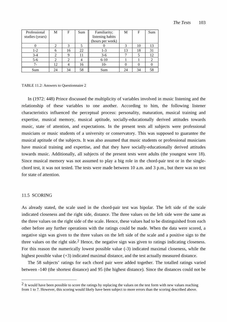
The Tests 103
Professional studies (years)
M F Sum Familiarity; listening habits
(hours per week)
M F Sum
0 2 3 5 0 3 10 13 1-2 6 16 22 1-3 13 18 31 3-4 2 9 11 3-6 7 5 12 5-6 2 2 4 6-10 1 1 2 7- 12 4 16 10- 0 0 0
Sum 24 34 58 Sum 24 34 58
TABLE 11.2: Answers to Questionnaire 2 In (1972: 448) Prince discussed the multiplicity of variables involved in music listening and the
relationship of these variables to one another. According to him, the following listener characteristics influenced the perceptual process: personality, maturation, musical training and expertise, musical memory, musical aptitude, socially-educationally derived attitudes towards music, state of attention, and expectations. In the present tests all subjects were professional musicians or music students of a university or conservatory. This was supposed to guarantee the musical aptitude of the subjects. It was also assumed that music students or professional musicians have musical training and expertise, and that they have socially-educationally derived attitudes towards music. Additionally, all subjects of the present tests were adults (the youngest were 18). Since musical memory was not assumed to play a big role in the chord-pair test or in the single-chord test, it was not tested. The tests were made between 10 a.m. and 3 p.m., but there was no test for state of attention.
11.5 SCORING
As already stated, the scale used in the chord-pair test was bipolar. The left side of the scale indicated closeness and the right side, distance. The three values on the left side were the same as the three values on the right side of the scale. Hence, these values had to be distinguished from each other before any further operations with the ratings could be made. When the data were scored, a negative sign was given to the three values on the left side of the scale and a positive sign to the three values on the right side.2 Hence, the negative sign was given to ratings indicating closeness. For this reason the numerically lowest possible value (-3) indicated maximal closeness, while the highest possible value (+3) indicated maximal distance, and the test actually measured distance.
The 58 subjects’ ratings for each chord pair were added together. The totalled ratings varied between -140 (the shortest distance) and 95 (the highest distance). Since the distances could not be
2 It would have been possible to score the ratings by replacing the values on the test form with new values reaching from 1 to 7. However, this scoring would likely have been subject to more errors than the scoring described above.
104 Chapter 11
negative, the original distances were modified to new values reaching from 0 to 23.5 (the linear transformation was made by the formula (x+140)/10). It should be noted that the original neutral value 0 was modified to 14. The distances were gathered into a distance matrix (see Table A 12.1 in Appendix 5).
The semantic scales on which the single chords were rated were similar to those used in the chord-pair test: bipolar and having three values on both sides of the scale. Again, the opposite values had to be distinguished from each other. For this reason, negative signs were given to the three values on the left side of each scale. Hence, negative signs were given to the following characteristics of the nine scales: rough, volatile, sparse, blurred, gloomy, angular, colourless, barren, and irritable. The arithmetic mean and the standard deviation of the subjects’ ratings of each chord on each scale was calculated. These values are given in Table A 13.1 in Appendix 5.
105
PART IV RESULTS AND CONCLUSIONS
The fourth and last part of the study analyzes the different datasets and describes the results that were obtained in these analyses. The chord-pair dataset is analyzed in Chapter 12 and the single-chord dataset in Chapter 13. The nine pentad-class datasets are analyzed in Chapter 14. Chapter 15 is a summary of the study, also offering the conclusions.

CHAPTER TWELVE RESULTS I: THE CHORD-PAIR DATASET
This chapter deals with the results that were obtained when the chord-pair dataset was analyzed. The dataset collected in the chord-pair test consisted of the subjects’ ratings of chord pairs on the scale ‘closeness - distance’. There were 75 pentachord pairs in the chord-pair test. As stated in Section 10.1, 66 chord pairs were derived from the 66 set-class pairs (pairwise comparisons of twelve pentad classes). The term ‘chord-pair dataset’ refers to the subjects’ ratings of these 66 chord pairs. Additionally, three pairs were played twice during the test. The term ‘control-chord pairs’ refers to these pairs. Each of the remaining six pairs consisted of two chords derived from the same set-class. However, these six pairs proved to be too few in number to be analyzed. Hence, they were excluded from further analyses.
Section 12.1 discusses the reliability of the subjects’ closeness ratings. The connection between closeness ratings and the number of common pitches in the chord pairs is discussed in Section 12.2. Section 12.3 deals with the connection between the nine pentad-class datasets and the chord-pair dataset. Closeness ratings made by some subject subgroups are analyzed in Section 12.4. Section 12.5 gives the multidimensional scaling analysis from the chord-pair dataset. The most important results are summarised in Section 12.6.
12.1 RELIABILITY OF THE SUBJECTS’ RATINGS
The reliability of the subjects’ ratings was tested by two analyses, first, by analyzing the ratings for the control-chord pairs, and second, by comparing each subject’s score to the score of all the other subjects. This section discusses these two analyses.
The control-chord test was made to find out how consistently the subjects rated closeness between two chords of a certain chord pair in different parts of the test. Each of the three test-pairs was first presented in the middle of the test, and then at the end of the test. Exactly the same
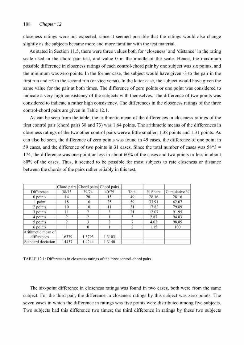
108 Chapter 12
closeness ratings were not expected, since it seemed possible that the ratings would also change slightly as the subjects became more and more familiar with the test material.
As stated in Section 11.5, there were three values both for ‘closeness’ and ‘distance’ in the rating scale used in the chord-pair test, and value 0 in the middle of the scale. Hence, the maximum possible difference in closeness ratings of each control-chord pair by one subject was six points, and the minimum was zero points. In the former case, the subject would have given -3 to the pair in the first run and +3 in the second run (or vice versa). In the latter case, the subject would have given the same value for the pair at both times. The difference of zero points or one point was considered to indicate a very high consistency of the subjects with themselves. The difference of two points was considered to indicate a rather high consistency. The differences in the closeness ratings of the three control-chord pairs are given in Table 12.1.
As can be seen from the table, the arithmetic mean of the differences in closeness ratings of the first control pair (chord pairs 38 and 73) was 1.64 points. The arithmetic means of the differences in closeness ratings of the two other control pairs were a little smaller, 1.38 points and 1.31 points. As can also be seen, the difference of zero points was found in 49 cases, the difference of one point in 59 cases, and the difference of two points in 31 cases. Since the total number of cases was 58*3 = 174, the difference was one point or less in about 60% of the cases and two points or less in about 80% of the cases. Thus, it seemed to be possible for most subjects to rate closeness or distance between the chords of the pairs rather reliably in this test.
Chord pairs Chord pairs Chord pairs Difference 38/73 39/74 40/75 Total % Share Cumulative %
0 points 14 20 15 49 28.16 28.16 1 point 18 16 25 59 33.91 62.07 2 points 10 10 11 31 17.82 79.89 3 points 11 7 3 21 12.07 91.95 4 points 2 2 1 5 2.87 94.83 5 points 2 3 2 7 4.02 98.85 6 points 1 0 1 2 1.15 100
Arithmetic mean of differences 1.6379 1.3793 1.3103
Standard deviation 1.4437 1.4244 1.3140
TABLE 12.1: Differences in closeness ratings of the three control-chord pairs
The six-point difference in closeness ratings was found in two cases, both were from the same
subject. For the third pair, the difference in closeness ratings by this subject was zero points. The seven cases in which the difference in ratings was five points were distributed among five subjects. Two subjects had this difference two times; the third difference in ratings by these two subjects
Results I 109
were three points and zero points. These two subjects, together with the one with the six-point differences, did not seem to rate the chord pairs very consistently.
In the second analysis, each individual subject’s score was compared to the score of all other subjects by calculating correlations between the closeness ratings from each subject and the sum of the ratings from the remaining subjects. This was done to find out subjects who had rated the pairs inconsistently in regard to other subjects. The correlations varied between -0.05 and 0.77 (N = 66), and for 53 subjects they were higher than 0.32 (and the p-values were lower than .010).1 Hence, most subjects rated the chord pairs consistently with the other subjects. There were five subjects for whom the correlation was lower than 0.32. These low correlations indicated that these five subjects did not rate the chord pairs consistently with other subjects. Additionally, one of these five subjects had low consistency in the control-chord test as well. Hence, the reliability of this subject’s ratings seemed questionable. The total difference in the control-chord test for the other four subjects varied between one and six points. It was thus possible that these four subjects used the scales in a different way from the other subjects, but consistently with themselves.
The analyses of the chord-pair dataset were made separately for three groups of subjects. The first group consisted of all subjects. The second group consisted of all but the subject who had low consistency with herself and with the other subjects. The third group consisted of all but the three subjects who had low consistency with themselves. Because the results were nearly equal in all cases, all data were used.
12.2 THE CONNECTION BETWEEN CLOSENESS RATINGS AND THE NUMBER OF COMMON PITCHES IN THE CHORD PAIRS
One factor influencing the closeness ratings seemed to be the number of common pitches between the two chords of one pair. The correlation was calculated between the subjects’ ratings of each pair and the number of common pitches in each pair. A rather high correlation (r = -0.66, p < .001) was found. This negative correlation indicated that increasing number of common pitches between two chords was connected with increasing estimated closeness (actually, decreasing distance) between the chords.2
In 26 pairs the chords had four pitches in common and one non-common pitch. The interval between the non-common pitch of chord 1 and the non-common pitch of chord 2 varied from one semitone to eleven semitones in the 26 pairs. The correlation was calculated between the interval in semitones in each of these pairs and the subjects’ ratings of the pairs. The correlation was very low, r = 0.20. Hence, this interval did not seem to affect the subjects’ ratings. 1 For p-values, see the entry ‘significance level’ in Definitions II. 2 As stated in Section 11.5, the ratings were scored so that the lowest (negative) ratings indicated closeness and the highest (positive) ratings indicated distance.
110 Chapter 12
In the remaining pairs (N = 40) the chords had three pitches in common. Hence, there were two non-common pitches in these pairs. The interval between the lower non-common pitch of chord 1 and the lower non-common pitch of chord 2 was added to the interval between the upper non-common pitch of chord 1 and the upper non-common pitch of chord 2. The sum of intervals thus obtained varied from two to sixteen semitones. This sum of intervals seemed to affect the subjects’ closeness ratings to some extent. The correlation between the sum of the intervals in semitones in each of the 40 pairs and the closeness ratings of the pairs was r = 0.57 (p < .001). This indicated that the chords were rated as being less close to each other as the sum of the intervals between the non-common pitches increased. Hence, it seemed that the number of common pitches was a factor guiding perception of closeness, but the intervals between the non-common pitches seemed to be important only when there were two non-common pitches in the pair.
12.3 THE CONNECTION BETWEEN MEASURED SIMILARITY AND PERCEIVED CLOSENESS
The correlations were calculated between the chord-pair dataset (subjects’ ratings of the 66 pentachord pairs) and each of the nine pentad-class datasets (similarity values as percentiles for the 66 set-class pairs).3 These correlations were calculated for one measure at a time (see Table 12.2). All correlations were statistically very significant (p ≤ .001), which indicated that the correlations were not occurring by chance. The highest correlations between measured similarity and closeness ratings were found for three total measures, namely, REL-% (r = 0.62), RECREL-% (r = 0.59), and ATMEMB-% (r = 0.58). The correlation between the ratings and the percentiles by the fourth total measure, AvgSATSIM-%, was lower, r = 0.45, this correlation being closer to the correlations for the other saturation-based measures (SATSIM-%, r = 0.40; and CSATSIM-%, r = 0.42) than for the other total measures. The highest correlation for interval-class vector-based measures was r = 0.52 for Cosθ-%. The lowest correlations were r = 0.39 for ASIM-% and r = 0.40 for SATSIM-%.
3 For percentiles, see Section 8.2. As stated in Section 9.4, the percentiles were the same for Cosθ and IcVD2; hence, Cosθ-% was selected to represent both measures.
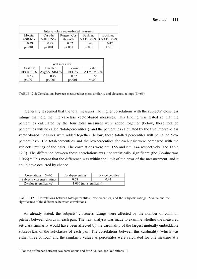
Results I 111
Interval-class vector-based measures Morris: ASIM-%
Castrén: %REL2-%
Rogers: Cos-theta-%
Buchler: SATSIM-%
Buchler: CSATSIM-%
0.39 p=.001
0.47 p<.001
0.52 p<.001
0.40 p=.001
0.42 p<.001
Total measures Castrén:
RECREL-% Buchler:
AvgSATSIM-% Lewin: REL-%
Rahn: ATMEMB-%
0.59 p<.001
0.45 p<.001
0.62 p<.001
0.58 p<.001
TABLE 12.2: Correlations between measured set-class similarity and closeness ratings (N=66).
Generally it seemed that the total measures had higher correlations with the subjects’ closeness
ratings than did the interval-class vector-based measures. This finding was tested so that the percentiles calculated by the four total measures were added together (below, these totalled percentiles will be called ‘total-percentiles’), and the percentiles calculated by the five interval-class vector-based measures were added together (below, these totalled percentiles will be called ‘icv-percentiles’). The total-percentiles and the icv-percentiles for each pair were compared with the subjects’ ratings of the pairs. The correlations were r = 0.58 and r = 0.44 respectively (see Table 12.3). The difference between these correlations was not statistically significant (the Z-value was 1.066).4 This meant that the difference was within the limit of the error of the measurement, and it could have occurred by chance.
Correlations N=66 Total-percentiles Icv-percentiles
Subjects' closeness ratings 0.58 0.44 Z-value (significance) 1.066 (not significant)
TABLE 12.3: Correlations between total-percentiles, icv-percentiles, and the subjects’ ratings. Z-value and the significance of the difference between correlations.
As already stated, the subjects’ closeness ratings were affected by the number of common
pitches between chords in each pair. The next analysis was made to examine whether the measured set-class similarity would have been affected by the cardinality of the largest mutually embeddable subset-class of the set-classes of each pair. The correlations between this cardinality (which was either three or four) and the similarity values as percentiles were calculated for one measure at a
4 For the difference between two correlations and for Z-values, see Definitions III.
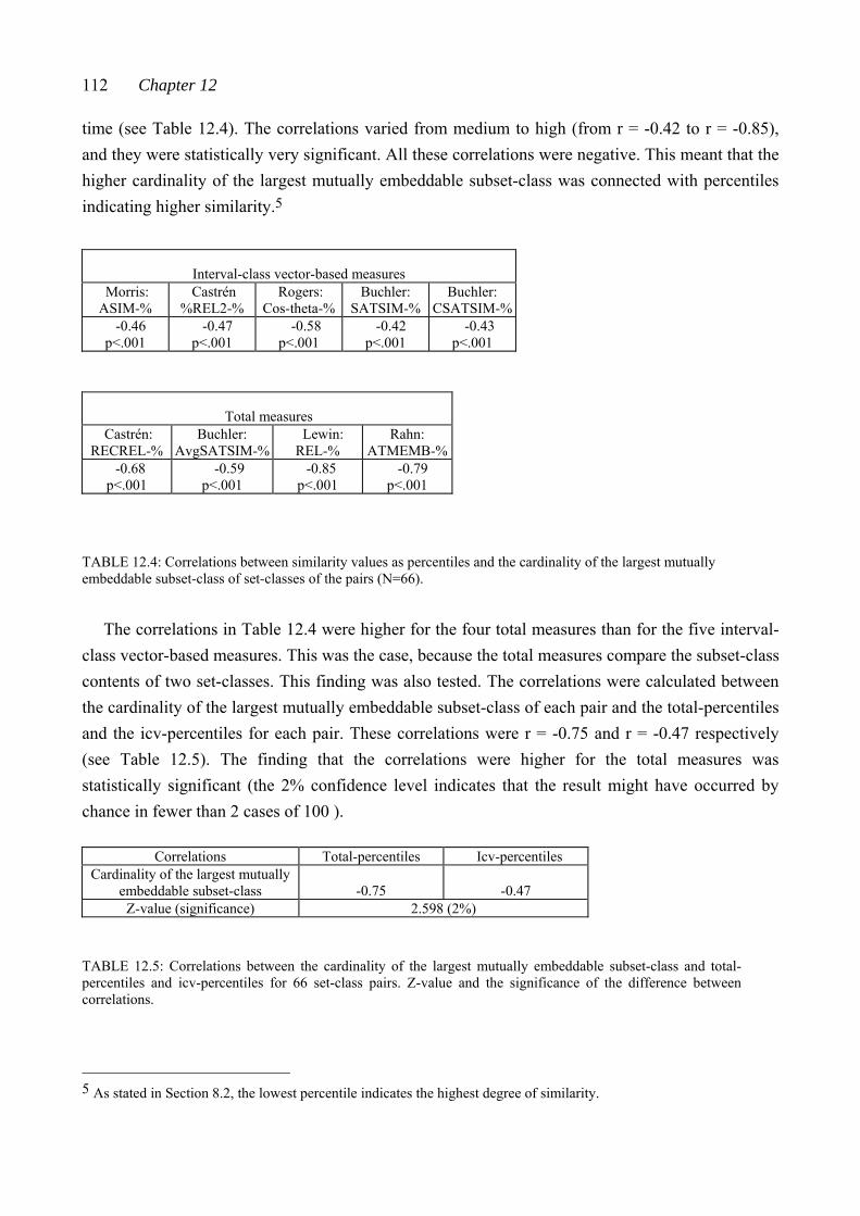
112 Chapter 12
time (see Table 12.4). The correlations varied from medium to high (from r = -0.42 to r = -0.85), and they were statistically very significant. All these correlations were negative. This meant that the higher cardinality of the largest mutually embeddable subset-class was connected with percentiles indicating higher similarity.5
Interval-class vector-based measures Morris: ASIM-%
Castrén %REL2-%
Rogers: Cos-theta-%
Buchler: SATSIM-%
Buchler: CSATSIM-%
-0.46 p<.001
-0.47 p<.001
-0.58 p<.001
-0.42 p<.001
-0.43 p<.001
Total measures Castrén:
RECREL-% Buchler:
AvgSATSIM-% Lewin: REL-%
Rahn: ATMEMB-%
-0.68 p<.001
-0.59 p<.001
-0.85 p<.001
-0.79 p<.001
TABLE 12.4: Correlations between similarity values as percentiles and the cardinality of the largest mutually embeddable subset-class of set-classes of the pairs (N=66).
The correlations in Table 12.4 were higher for the four total measures than for the five interval-
class vector-based measures. This was the case, because the total measures compare the subset-class contents of two set-classes. This finding was also tested. The correlations were calculated between the cardinality of the largest mutually embeddable subset-class of each pair and the total-percentiles and the icv-percentiles for each pair. These correlations were r = -0.75 and r = -0.47 respectively (see Table 12.5). The finding that the correlations were higher for the total measures was statistically significant (the 2% confidence level indicates that the result might have occurred by chance in fewer than 2 cases of 100 ).
Correlations Total-percentiles Icv-percentiles
Cardinality of the largest mutually embeddable subset-class -0.75 -0.47 Z-value (significance) 2.598 (2%)
TABLE 12.5: Correlations between the cardinality of the largest mutually embeddable subset-class and total-percentiles and icv-percentiles for 66 set-class pairs. Z-value and the significance of the difference between correlations.
5 As stated in Section 8.2, the lowest percentile indicates the highest degree of similarity.
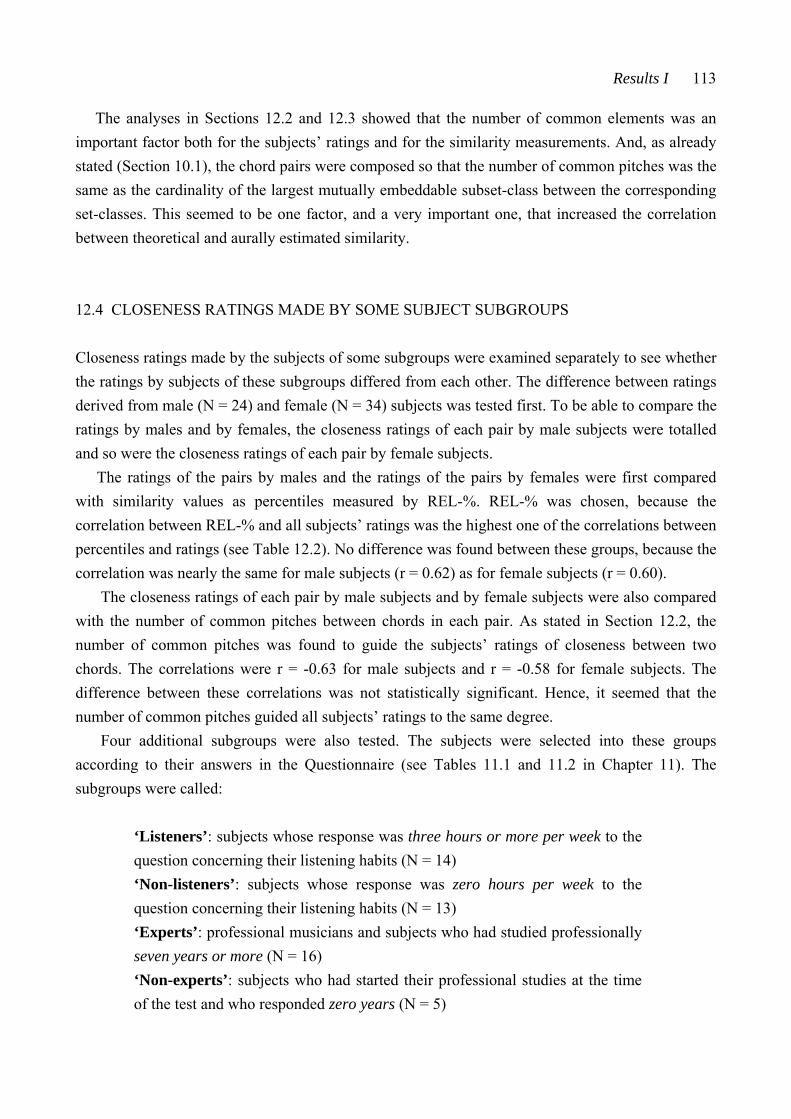
Results I 113
The analyses in Sections 12.2 and 12.3 showed that the number of common elements was an important factor both for the subjects’ ratings and for the similarity measurements. And, as already stated (Section 10.1), the chord pairs were composed so that the number of common pitches was the same as the cardinality of the largest mutually embeddable subset-class between the corresponding set-classes. This seemed to be one factor, and a very important one, that increased the correlation between theoretical and aurally estimated similarity.
12.4 CLOSENESS RATINGS MADE BY SOME SUBJECT SUBGROUPS
Closeness ratings made by the subjects of some subgroups were examined separately to see whether the ratings by subjects of these subgroups differed from each other. The difference between ratings derived from male (N = 24) and female (N = 34) subjects was tested first. To be able to compare the ratings by males and by females, the closeness ratings of each pair by male subjects were totalled and so were the closeness ratings of each pair by female subjects.
The ratings of the pairs by males and the ratings of the pairs by females were first compared with similarity values as percentiles measured by REL-%. REL-% was chosen, because the correlation between REL-% and all subjects’ ratings was the highest one of the correlations between percentiles and ratings (see Table 12.2). No difference was found between these groups, because the correlation was nearly the same for male subjects (r = 0.62) as for female subjects (r = 0.60).
The closeness ratings of each pair by male subjects and by female subjects were also compared with the number of common pitches between chords in each pair. As stated in Section 12.2, the number of common pitches was found to guide the subjects’ ratings of closeness between two chords. The correlations were r = -0.63 for male subjects and r = -0.58 for female subjects. The difference between these correlations was not statistically significant. Hence, it seemed that the number of common pitches guided all subjects’ ratings to the same degree.
Four additional subgroups were also tested. The subjects were selected into these groups according to their answers in the Questionnaire (see Tables 11.1 and 11.2 in Chapter 11). The subgroups were called:
‘Listeners’: subjects whose response was three hours or more per week to the question concerning their listening habits (N = 14) ‘Non-listeners’: subjects whose response was zero hours per week to the question concerning their listening habits (N = 13) ‘Experts’: professional musicians and subjects who had studied professionally seven years or more (N = 16) ‘Non-experts’: subjects who had started their professional studies at the time of the test and who responded zero years (N = 5)
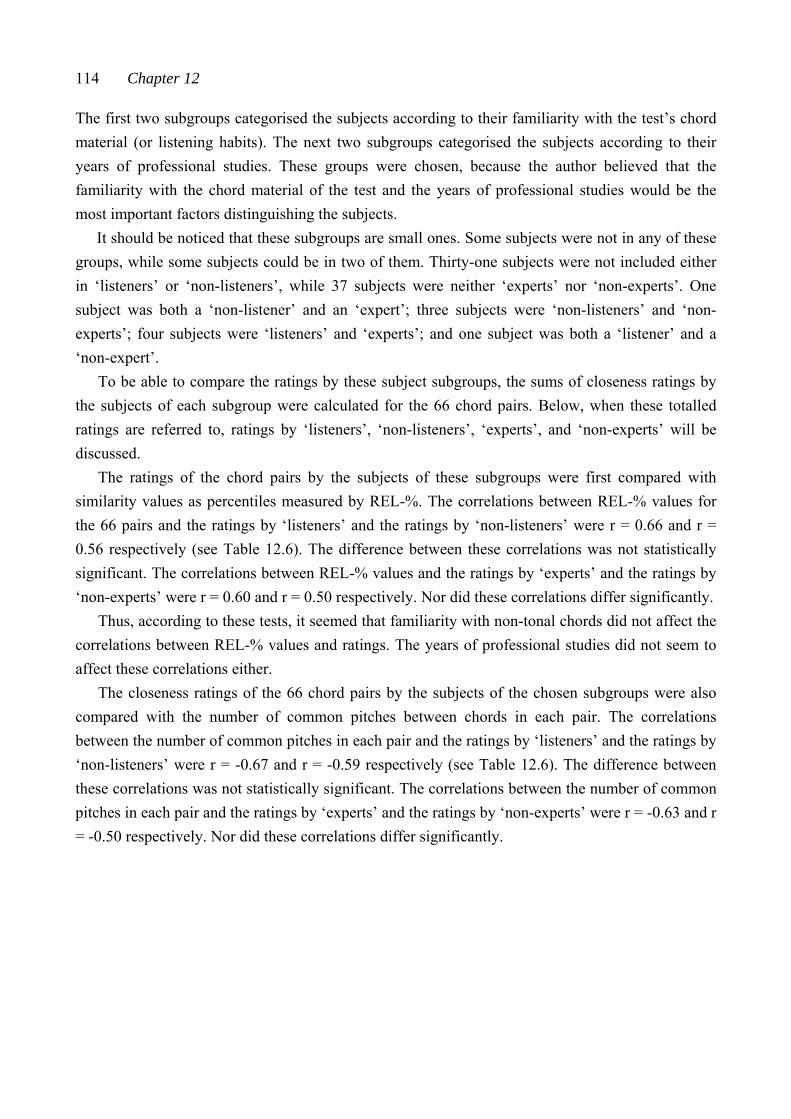
114 Chapter 12
The first two subgroups categorised the subjects according to their familiarity with the test’s chord material (or listening habits). The next two subgroups categorised the subjects according to their years of professional studies. These groups were chosen, because the author believed that the familiarity with the chord material of the test and the years of professional studies would be the most important factors distinguishing the subjects.
It should be noticed that these subgroups are small ones. Some subjects were not in any of these groups, while some subjects could be in two of them. Thirty-one subjects were not included either in ‘listeners’ or ‘non-listeners’, while 37 subjects were neither ‘experts’ nor ‘non-experts’. One subject was both a ‘non-listener’ and an ‘expert’; three subjects were ‘non-listeners’ and ‘non-experts’; four subjects were ‘listeners’ and ‘experts’; and one subject was both a ‘listener’ and a ‘non-expert’.
To be able to compare the ratings by these subject subgroups, the sums of closeness ratings by the subjects of each subgroup were calculated for the 66 chord pairs. Below, when these totalled ratings are referred to, ratings by ‘listeners’, ‘non-listeners’, ‘experts’, and ‘non-experts’ will be discussed.
The ratings of the chord pairs by the subjects of these subgroups were first compared with similarity values as percentiles measured by REL-%. The correlations between REL-% values for the 66 pairs and the ratings by ‘listeners’ and the ratings by ‘non-listeners’ were r = 0.66 and r = 0.56 respectively (see Table 12.6). The difference between these correlations was not statistically significant. The correlations between REL-% values and the ratings by ‘experts’ and the ratings by ‘non-experts’ were r = 0.60 and r = 0.50 respectively. Nor did these correlations differ significantly.
Thus, according to these tests, it seemed that familiarity with non-tonal chords did not affect the correlations between REL-% values and ratings. The years of professional studies did not seem to affect these correlations either.
The closeness ratings of the 66 chord pairs by the subjects of the chosen subgroups were also compared with the number of common pitches between chords in each pair. The correlations between the number of common pitches in each pair and the ratings by ‘listeners’ and the ratings by ‘non-listeners’ were r = -0.67 and r = -0.59 respectively (see Table 12.6). The difference between these correlations was not statistically significant. The correlations between the number of common pitches in each pair and the ratings by ‘experts’ and the ratings by ‘non-experts’ were r = -0.63 and r = -0.50 respectively. Nor did these correlations differ significantly.
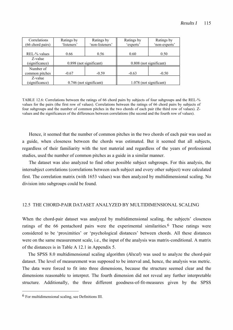
Results I 115
Correlations
(66 chord pairs) Ratings by ‘listeners’
Ratings by ‘non-listeners’
Ratings by ‘experts’
Ratings by ‘non-experts’
REL-% values
0.66
0.56
0.60
0.50
Z-value (significance) 0.898 (not significant) 0.808 (not significant)
Number of common pitches -0.67 -0.59 -0.63 -0.50
Z-value (significance) 0.746 (not significant) 1.078 (not significant)
TABLE 12.6: Correlations between the ratings of 66 chord pairs by subjects of four subgroups and the REL-% values for the pairs (the first row of values). Correlations between the ratings of 66 chord pairs by subjects of four subgroups and the number of common pitches in the two chords of each pair (the third row of values). Z-values and the significances of the differences between correlations (the second and the fourth row of values).
Hence, it seemed that the number of common pitches in the two chords of each pair was used as a guide, when closeness between the chords was estimated. But it seemed that all subjects, regardless of their familiarity with the test material and regardless of the years of professional studies, used the number of common pitches as a guide in a similar manner.
The dataset was also analyzed to find other possible subject subgroups. For this analysis, the intersubject correlations (correlations between each subject and every other subject) were calculated first. The correlation matrix (with 1653 values) was then analyzed by multidimensional scaling. No division into subgroups could be found.
12.5 THE CHORD-PAIR DATASET ANALYZED BY MULTIDIMENSIONAL SCALING
When the chord-pair dataset was analyzed by multidimensional scaling, the subjects’ closeness ratings of the 66 pentachord pairs were the experimental similarities.6 These ratings were considered to be ‘proximities’ or ‘psychological distances’ between chords. All these distances were on the same measurement scale, i.e., the input of the analysis was matrix-conditional. A matrix of the distances is in Table A 12.1 in Appendix 5.
The SPSS 8.0 multidimensional scaling algorithm (Alscal) was used to analyze the chord-pair dataset. The level of measurement was supposed to be interval and, hence, the analysis was metric. The data were forced to fit into three dimensions, because the structure seemed clear and the dimensions reasonable to interpret. The fourth dimension did not reveal any further interpretable structure. Additionally, the three different goodness-of-fit-measures given by the SPSS
6 For multidimensional scaling, see Definitions III.
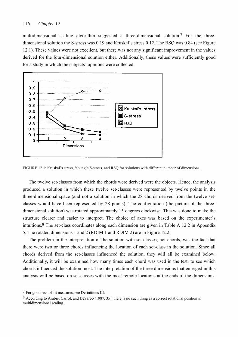
116 Chapter 12
multidimensional scaling algorithm suggested a three-dimensional solution.7 For the three-dimensional solution the S-stress was 0.19 and Kruskal’s stress 0.12. The RSQ was 0.84 (see Figure 12.1). These values were not excellent, but there was not any significant improvement in the values derived for the four-dimensional solution either. Additionally, these values were sufficiently good for a study in which the subjects’ opinions were collected.
FIGURE 12.1: Kruskal’s stress, Young’s S-stress, and RSQ for solutions with different number of dimensions.
The twelve set-classes from which the chords were derived were the objects. Hence, the analysis
produced a solution in which these twelve set-classes were represented by twelve points in the three-dimensional space (and not a solution in which the 28 chords derived from the twelve set-classes would have been represented by 28 points). The configuration (the picture of the three-dimensional solution) was rotated approximately 15 degrees clockwise. This was done to make the structure clearer and easier to interpret. The choice of axes was based on the experimenter’s intuitions.8 The set-class coordinates along each dimension are given in Table A 12.2 in Appendix 5. The rotated dimensions 1 and 2 (RDIM 1 and RDIM 2) are in Figure 12.2.
The problem in the interpretation of the solution with set-classes, not chords, was the fact that there were two or three chords influencing the location of each set-class in the solution. Since all chords derived from the set-classes influenced the solution, they will all be examined below. Additionally, it will be examined how many times each chord was used in the test, to see which chords influenced the solution most. The interpretation of the three dimensions that emerged in this analysis will be based on set-classes with the most remote locations at the ends of the dimensions.
7 For goodness-of-fit measures, see Definitions III. 8 According to Arabie, Carrol, and DeSarbo (1987: 35), there is no such thing as a correct rotational position in multidimensional scaling.
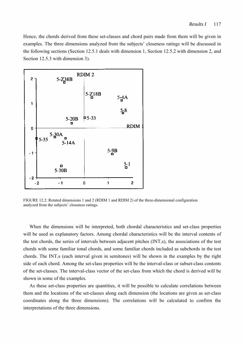
Results I 117
Hence, the chords derived from these set-classes and chord pairs made from them will be given in examples. The three dimensions analyzed from the subjects’ closeness ratings will be discussed in the following sections (Section 12.5.1 deals with dimension 1, Section 12.5.2 with dimension 2, and Section 12.5.3 with dimension 3).
FIGURE 12.2: Rotated dimensions 1 and 2 (RDIM 1 and RDIM 2) of the three-dimensional configuration analyzed from the subjects’ closeness ratings.
When the dimensions will be interpreted, both chordal characteristics and set-class properties
will be used as explanatory factors. Among chordal characteristics will be the interval contents of the test chords, the series of intervals between adjacent pitches (INT1s), the associations of the test chords with some familiar tonal chords, and some familiar chords included as subchords in the test chords. The INT1s (each interval given in semitones) will be shown in the examples by the right side of each chord. Among the set-class properties will be the interval-class or subset-class contents of the set-classes. The interval-class vector of the set-class from which the chord is derived will be shown in some of the examples.
As these set-class properties are quantities, it will be possible to calculate correlations between them and the locations of the set-classes along each dimension (the locations are given as set-class coordinates along the three dimensions). The correlations will be calculated to confirm the interpretations of the three dimensions.
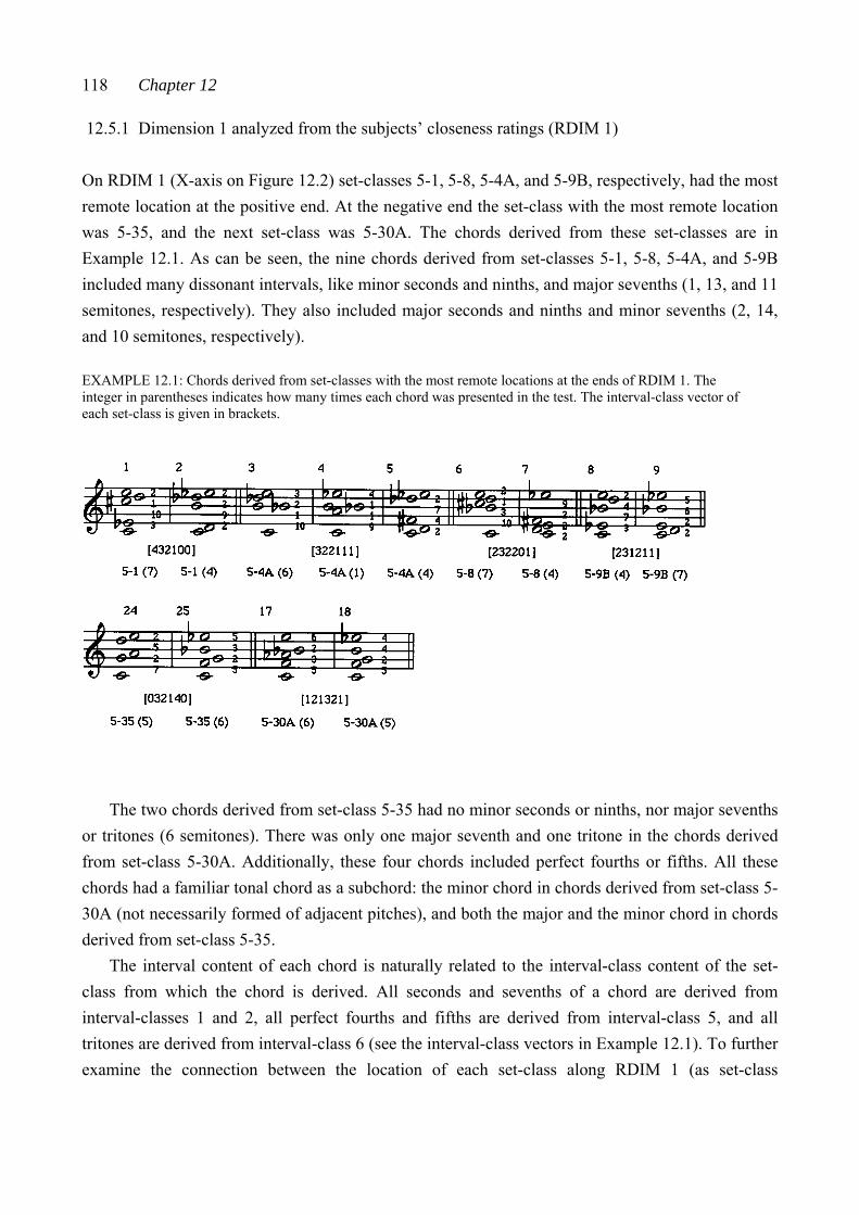
118 Chapter 12
12.5.1 Dimension 1 analyzed from the subjects’ closeness ratings (RDIM 1)
On RDIM 1 (X-axis on Figure 12.2) set-classes 5-1, 5-8, 5-4A, and 5-9B, respectively, had the most remote location at the positive end. At the negative end the set-class with the most remote location was 5-35, and the next set-class was 5-30A. The chords derived from these set-classes are in Example 12.1. As can be seen, the nine chords derived from set-classes 5-1, 5-8, 5-4A, and 5-9B included many dissonant intervals, like minor seconds and ninths, and major sevenths (1, 13, and 11 semitones, respectively). They also included major seconds and ninths and minor sevenths (2, 14, and 10 semitones, respectively).
EXAMPLE 12.1: Chords derived from set-classes with the most remote locations at the ends of RDIM 1. The integer in parentheses indicates how many times each chord was presented in the test. The interval-class vector of each set-class is given in brackets.
The two chords derived from set-class 5-35 had no minor seconds or ninths, nor major sevenths or tritones (6 semitones). There was only one major seventh and one tritone in the chords derived from set-class 5-30A. Additionally, these four chords included perfect fourths or fifths. All these chords had a familiar tonal chord as a subchord: the minor chord in chords derived from set-class 5-30A (not necessarily formed of adjacent pitches), and both the major and the minor chord in chords derived from set-class 5-35.
The interval content of each chord is naturally related to the interval-class content of the set-class from which the chord is derived. All seconds and sevenths of a chord are derived from interval-classes 1 and 2, all perfect fourths and fifths are derived from interval-class 5, and all tritones are derived from interval-class 6 (see the interval-class vectors in Example 12.1). To further examine the connection between the location of each set-class along RDIM 1 (as set-class
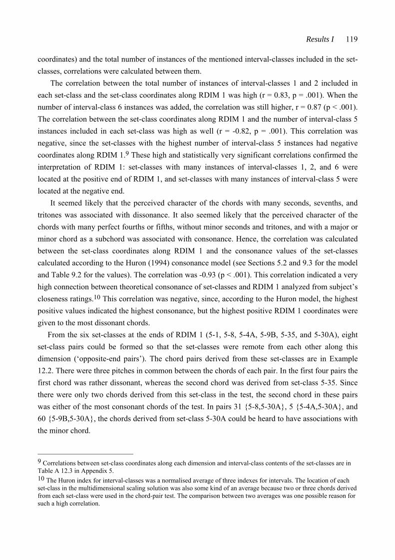
Results I 119
coordinates) and the total number of instances of the mentioned interval-classes included in the set-classes, correlations were calculated between them.
The correlation between the total number of instances of interval-classes 1 and 2 included in each set-class and the set-class coordinates along RDIM 1 was high (r = 0.83, p = .001). When the number of interval-class 6 instances was added, the correlation was still higher, r = 0.87 (p < .001). The correlation between the set-class coordinates along RDIM 1 and the number of interval-class 5 instances included in each set-class was high as well (r = -0.82, p = .001). This correlation was negative, since the set-classes with the highest number of interval-class 5 instances had negative coordinates along RDIM 1.9 These high and statistically very significant correlations confirmed the interpretation of RDIM 1: set-classes with many instances of interval-classes 1, 2, and 6 were located at the positive end of RDIM 1, and set-classes with many instances of interval-class 5 were located at the negative end.
It seemed likely that the perceived character of the chords with many seconds, sevenths, and tritones was associated with dissonance. It also seemed likely that the perceived character of the chords with many perfect fourths or fifths, without minor seconds and tritones, and with a major or minor chord as a subchord was associated with consonance. Hence, the correlation was calculated between the set-class coordinates along RDIM 1 and the consonance values of the set-classes calculated according to the Huron (1994) consonance model (see Sections 5.2 and 9.3 for the model and Table 9.2 for the values). The correlation was -0.93 (p < .001). This correlation indicated a very high connection between theoretical consonance of set-classes and RDIM 1 analyzed from subject’s closeness ratings.10 This correlation was negative, since, according to the Huron model, the highest positive values indicated the highest consonance, but the highest positive RDIM 1 coordinates were given to the most dissonant chords.
From the six set-classes at the ends of RDIM 1 (5-1, 5-8, 5-4A, 5-9B, 5-35, and 5-30A), eight set-class pairs could be formed so that the set-classes were remote from each other along this dimension (‘opposite-end pairs’). The chord pairs derived from these set-classes are in Example 12.2. There were three pitches in common between the chords of each pair. In the first four pairs the first chord was rather dissonant, whereas the second chord was derived from set-class 5-35. Since there were only two chords derived from this set-class in the test, the second chord in these pairs was either of the most consonant chords of the test. In pairs 31 {5-8,5-30A}, 5 {5-4A,5-30A}, and 60 {5-9B,5-30A}, the chords derived from set-class 5-30A could be heard to have associations with the minor chord.
9 Correlations between set-class coordinates along each dimension and interval-class contents of the set-classes are in Table A 12.3 in Appendix 5. 10 The Huron index for interval-classes was a normalised average of three indexes for intervals. The location of each set-class in the multidimensional scaling solution was also some kind of an average because two or three chords derived from each set-class were used in the chord-pair test. The comparison between two averages was one possible reason for such a high correlation.
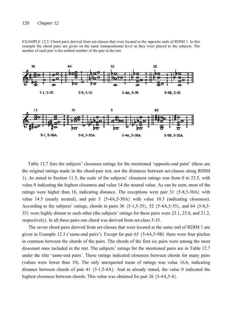
120 Chapter 12
EXAMPLE 12.2: Chord pairs derived from set-classes that were located at the opposite ends of RDIM 1. In this example the chord pairs are given on the same transpositional level as they were played to the subjects. The number of each pair is the ordinal number of the pair in the test.
Table 12.7 lists the subjects’ closeness ratings for the mentioned ‘opposite-end pairs’ (these are
the original ratings made in the chord-pair test, not the distances between set-classes along RDIM 1). As stated in Section 11.5, the scale of the subjects’ closeness ratings was from 0 to 23.5, with value 0 indicating the highest closeness and value 14 the neutral value. As can be seen, most of the ratings were higher than 16, indicating distance. The exceptions were pair 31 {5-8,5-30A} with value 14.5 (nearly neutral), and pair 5 {5-4A,5-30A} with value 10.3 (indicating closeness). According to the subjects’ ratings, chords in pairs 36 {5-1,5-35}, 52 {5-4A,5-35}, and 64 {5-8,5-35} were highly distant to each other (the subjects’ ratings for these pairs were 23.1, 23.0, and 21.2, respectively). In all these pairs one chord was derived from set-class 5-35.
The seven chord pairs derived from set-classes that were located at the same end of RDIM 1 are given in Example 12.3 (‘same-end pairs’). Except for pair 65 {5-4A,5-9B} there were four pitches in common between the chords of the pairs. The chords of the first six pairs were among the most dissonant ones included in the test. The subjects’ ratings for the mentioned pairs are in Table 12.7 under the title ‘same-end pairs’. These ratings indicated closeness between chords for many pairs (values were lower than 10). The only unexpected mean of ratings was value 16.6, indicating distance between chords of pair 41 {5-1,5-4A}. And as already stated, the value 0 indicated the highest closeness between chords. This value was obtained for pair 26 {5-4A,5-8}.
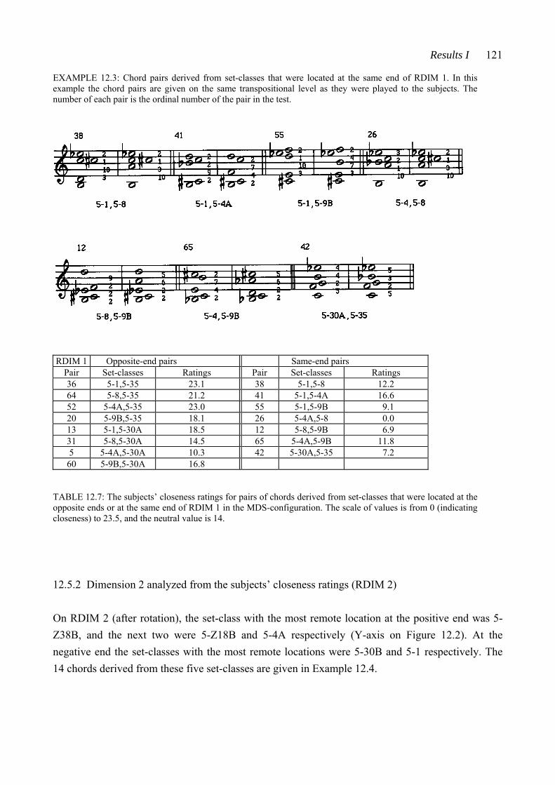
Results I 121
EXAMPLE 12.3: Chord pairs derived from set-classes that were located at the same end of RDIM 1. In this example the chord pairs are given on the same transpositional level as they were played to the subjects. The number of each pair is the ordinal number of the pair in the test.
RDIM 1 Opposite-end pairs Same-end pairs
Pair Set-classes Ratings Pair Set-classes Ratings 36 5-1,5-35 23.1 38 5-1,5-8 12.2 64 5-8,5-35 21.2 41 5-1,5-4A 16.6 52 5-4A,5-35 23.0 55 5-1,5-9B 9.1 20 5-9B,5-35 18.1 26 5-4A,5-8 0.0 13 5-1,5-30A 18.5 12 5-8,5-9B 6.9 31 5-8,5-30A 14.5 65 5-4A,5-9B 11.8 5 5-4A,5-30A 10.3 42 5-30A,5-35 7.2
60 5-9B,5-30A 16.8
TABLE 12.7: The subjects’ closeness ratings for pairs of chords derived from set-classes that were located at the opposite ends or at the same end of RDIM 1 in the MDS-configuration. The scale of values is from 0 (indicating closeness) to 23.5, and the neutral value is 14.
12.5.2 Dimension 2 analyzed from the subjects’ closeness ratings (RDIM 2)
On RDIM 2 (after rotation), the set-class with the most remote location at the positive end was 5-Z38B, and the next two were 5-Z18B and 5-4A respectively (Y-axis on Figure 12.2). At the negative end the set-classes with the most remote locations were 5-30B and 5-1 respectively. The 14 chords derived from these five set-classes are given in Example 12.4.

122 Chapter 12
EXAMPLE 12.4: Chords derived from set-classes with the most remote locations at the ends of RDIM 2. The integer in parentheses indicates how many times each chord was presented in the test. The interval-class vector of each set-class is given in brackets.
The chords derived from set-class 5-Z38B had clear associations with the dominant seventh
chord: the dominant seventh chord was a subchord in all these chords (the ‘extra’ pitch was E in chords 26 and 28, and B in chord 27). The dominant seventh chord with the minor ninth and without the fifth was a subchord in the chords derived from set-classes 5-Z18B and 5-4A. In these chords the ‘extra’ pitches were F in chord 12, G in chord 13, E in chord 14, B in chord 3, Bb in chord 4, and C# in chord 5. No associations with the dominant chord were obviously heard in chords derived from set-classes 5-30B or 5-1.
The perceived dominant ninth chord association was perhaps not very clear in chord 14 because of the minor sixth chord formed from the three lowest pitches. But chord 14 was used only once during the test; it was paired with chord 28 derived from set-class 5-Z38B (see pair 3 in Example 12.5). And the subjects’ ratings indicated closeness (short distance; 5.9) between these two chords (see Table 12.8, title ‘same-end pairs’, for the ratings).
The subjects’ closeness rating for pair 46 {5-4A,5-Z18B} was 2.1 (see Table 12.8), indicating high closeness. In this chord pair the two chords had reference to the same dominant seventh chord with the minor ninth and without the fifth (D, F#, C and Eb), with one ‘extra’ pitch in both chords (see Example 12.5). This obviously was one reason for the subjects’ ratings. Even though there were rather similar conditions in pair 57 {5-4A,5-Z38B} (the dominant seventh chord with the minor ninth and without the fifth in the first chord, and the dominant seventh chord in the second; the same root [B] and the same ‘extra’ pitch [A#] in both chords), the subjects’ ratings indicated distance between the chords (16.1).
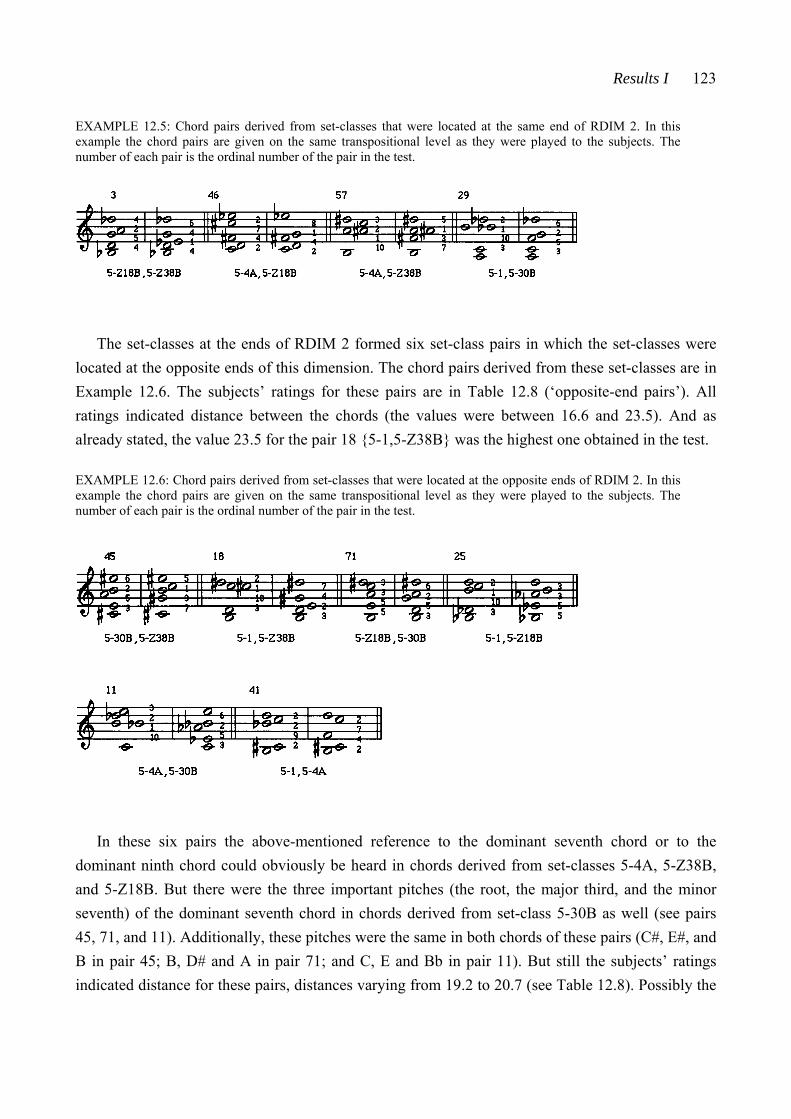
Results I 123
EXAMPLE 12.5: Chord pairs derived from set-classes that were located at the same end of RDIM 2. In this example the chord pairs are given on the same transpositional level as they were played to the subjects. The number of each pair is the ordinal number of the pair in the test.
The set-classes at the ends of RDIM 2 formed six set-class pairs in which the set-classes were
located at the opposite ends of this dimension. The chord pairs derived from these set-classes are in Example 12.6. The subjects’ ratings for these pairs are in Table 12.8 (‘opposite-end pairs’). All ratings indicated distance between the chords (the values were between 16.6 and 23.5). And as already stated, the value 23.5 for the pair 18 {5-1,5-Z38B} was the highest one obtained in the test.
EXAMPLE 12.6: Chord pairs derived from set-classes that were located at the opposite ends of RDIM 2. In this example the chord pairs are given on the same transpositional level as they were played to the subjects. The number of each pair is the ordinal number of the pair in the test.
In these six pairs the above-mentioned reference to the dominant seventh chord or to the dominant ninth chord could obviously be heard in chords derived from set-classes 5-4A, 5-Z38B, and 5-Z18B. But there were the three important pitches (the root, the major third, and the minor seventh) of the dominant seventh chord in chords derived from set-class 5-30B as well (see pairs 45, 71, and 11). Additionally, these pitches were the same in both chords of these pairs (C#, E#, and B in pair 45; B, D# and A in pair 71; and C, E and Bb in pair 11). But still the subjects’ ratings indicated distance for these pairs, distances varying from 19.2 to 20.7 (see Table 12.8). Possibly the
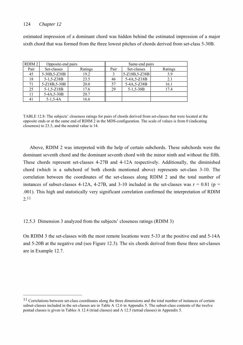
124 Chapter 12
estimated impression of a dominant chord was hidden behind the estimated impression of a major sixth chord that was formed from the three lowest pitches of chords derived from set-class 5-30B.
RDIM 2 Opposite-end pairs Same-end pairs Pair Set-classes Ratings Pair Set-classes Ratings 45 5-30B,5-Z38B 19.2 3 5-Z18B,5-Z38B 5.9 18 5-1,5-Z38B 23.5 46 5-4A,5-Z18B 2.1 71 5-Z18B,5-30B 20.0 57 5-4A,5-Z38B 16.1 25 5-1,5-Z18B 17.6 29 5-1,5-30B 17.4 11 5-4A,5-30B 20.7 41 5-1,5-4A 16.6
TABLE 12.8: The subjects’ closeness ratings for pairs of chords derived from set-classes that were located at the opposite ends or at the same end of RDIM 2 in the MDS-configuration. The scale of values is from 0 (indicating closeness) to 23.5, and the neutral value is 14.
Above, RDIM 2 was interpreted with the help of certain subchords. These subchords were the
dominant seventh chord and the dominant seventh chord with the minor ninth and without the fifth. These chords represent set-classes 4-27B and 4-12A respectively. Additionally, the diminished chord (which is a subchord of both chords mentioned above) represents set-class 3-10. The correlation between the coordinates of the set-classes along RDIM 2 and the total number of instances of subset-classes 4-12A, 4-27B, and 3-10 included in the set-classes was r = 0.81 (p = .001). This high and statistically very significant correlation confirmed the interpretation of RDIM 2.11
12.5.3 Dimension 3 analyzed from the subjects’ closeness ratings (RDIM 3)
On RDIM 3 the set-classes with the most remote locations were 5-33 at the positive end and 5-14A and 5-20B at the negative end (see Figure 12.3). The six chords derived from these three set-classes are in Example 12.7.
11 Correlations between set-class coordinates along the three dimensions and the total number of instances of certain subset-classes included in the set-classes are in Table A 12.6 in Appendix 5. The subset-class contents of the twelve pentad classes is given in Tables A 12.4 (triad classes) and A 12.5 (tetrad classes) in Appendix 5.
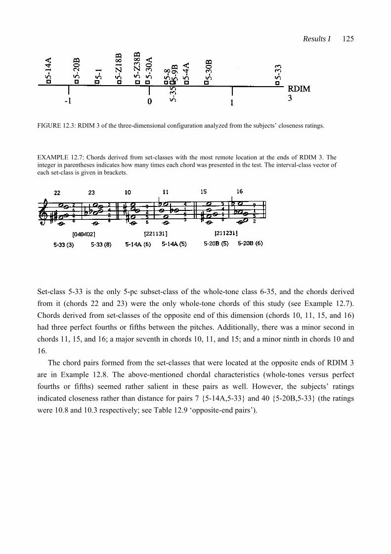
Results I 125
FIGURE 12.3: RDIM 3 of the three-dimensional configuration analyzed from the subjects’ closeness ratings.
EXAMPLE 12.7: Chords derived from set-classes with the most remote location at the ends of RDIM 3. The integer in parentheses indicates how many times each chord was presented in the test. The interval-class vector of each set-class is given in brackets.
Set-class 5-33 is the only 5-pc subset-class of the whole-tone class 6-35, and the chords derived from it (chords 22 and 23) were the only whole-tone chords of this study (see Example 12.7). Chords derived from set-classes of the opposite end of this dimension (chords 10, 11, 15, and 16) had three perfect fourths or fifths between the pitches. Additionally, there was a minor second in chords 11, 15, and 16; a major seventh in chords 10, 11, and 15; and a minor ninth in chords 10 and 16.
The chord pairs formed from the set-classes that were located at the opposite ends of RDIM 3 are in Example 12.8. The above-mentioned chordal characteristics (whole-tones versus perfect fourths or fifths) seemed rather salient in these pairs as well. However, the subjects’ ratings indicated closeness rather than distance for pairs 7 {5-14A,5-33} and 40 {5-20B,5-33} (the ratings were 10.8 and 10.3 respectively; see Table 12.9 ‘opposite-end pairs’).
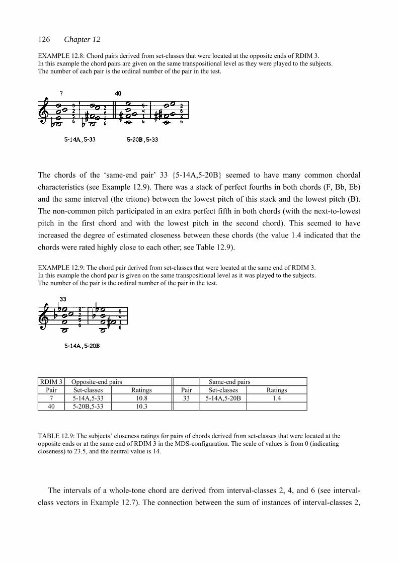
126 Chapter 12
EXAMPLE 12.8: Chord pairs derived from set-classes that were located at the opposite ends of RDIM 3. In this example the chord pairs are given on the same transpositional level as they were played to the subjects. The number of each pair is the ordinal number of the pair in the test.
The chords of the ‘same-end pair’ 33 {5-14A,5-20B} seemed to have many common chordal characteristics (see Example 12.9). There was a stack of perfect fourths in both chords (F, Bb, Eb) and the same interval (the tritone) between the lowest pitch of this stack and the lowest pitch (B). The non-common pitch participated in an extra perfect fifth in both chords (with the next-to-lowest pitch in the first chord and with the lowest pitch in the second chord). This seemed to have increased the degree of estimated closeness between these chords (the value 1.4 indicated that the chords were rated highly close to each other; see Table 12.9).
EXAMPLE 12.9: The chord pair derived from set-classes that were located at the same end of RDIM 3. In this example the chord pair is given on the same transpositional level as it was played to the subjects. The number of the pair is the ordinal number of the pair in the test.
RDIM 3 Opposite-end pairs Same-end pairs
Pair Set-classes Ratings Pair Set-classes Ratings 7 5-14A,5-33 10.8 33 5-14A,5-20B 1.4
40 5-20B,5-33 10.3 TABLE 12.9: The subjects’ closeness ratings for pairs of chords derived from set-classes that were located at the opposite ends or at the same end of RDIM 3 in the MDS-configuration. The scale of values is from 0 (indicating closeness) to 23.5, and the neutral value is 14.
The intervals of a whole-tone chord are derived from interval-classes 2, 4, and 6 (see interval-
class vectors in Example 12.7). The connection between the sum of instances of interval-classes 2,
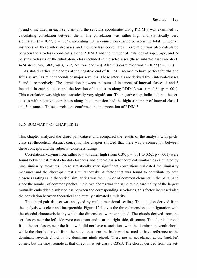
Results I 127
4, and 6 included in each set-class and the set-class coordinates along RDIM 3 was examined by calculating correlation between them. The correlation was rather high and statistically very significant (r = 0.77, p = .003), indicating that a connection existed between the total number of instances of these interval-classes and the set-class coordinates. Correlation was also calculated between the set-class coordinates along RDIM 3 and the number of instances of 4-pc, 3-pc, and 2-pc subset-classes of the whole-tone class included in the set-classes (these subset-classes are 4-21, 4-24, 4-25, 3-6, 3-8A, 3-8B, 3-12, 2-2, 2-4, and 2-6). Also this correlation was r = 0.77 (p = .003).
As stated earlier, the chords at the negative end of RDIM 3 seemed to have perfect fourths and fifths as well as minor seconds or major sevenths. These intervals are derived from interval-classes 5 and 1 respectively. The correlation between the sum of instances of interval-classes 1 and 5 included in each set-class and the location of set-classes along RDIM 3 was r = -0.84 (p = .001). This correlation was high and statistically very significant. The negative sign indicated that the set-classes with negative coordinates along this dimension had the highest number of interval-class 1 and 5 instances. These correlations confirmed the interpretation of RDIM 3.
12.6 SUMMARY OF CHAPTER 12
This chapter analyzed the chord-pair dataset and compared the results of the analysis with pitch-class set-theoretical abstract concepts. The chapter showed that there was a connection between these concepts and the subjects’ closeness ratings.
Correlations varying from rather low to rather high (from 0.39, p = .001 to 0.62, p < .001) were found between estimated chordal closeness and pitch-class set-theoretical similarities calculated by nine similarity measures. These statistically very significant correlations validated the similarity measures and the chord-pair test simultaneously. A factor that was found to contribute to both closeness ratings and theoretical similarities was the number of common elements in the pairs. And since the number of common pitches in the two chords was the same as the cardinality of the largest mutually embeddable subset-class between the corresponding set-classes, this factor increased also the correlation between theoretical and aurally estimated similarity.
The chord-pair dataset was analyzed by multidimensional scaling. The solution derived from the analysis was clear and interpretable. Figure 12.4 gives the three-dimensional configuration with the chordal characteristics by which the dimensions were explained. The chords derived from the set-classes near the left side were consonant and near the right side, dissonant. The chords derived from the set-classes near the front wall did not have associations with the dominant seventh chord, while the chords derived from the set-classes near the back wall seemed to have reference to the dominant seventh chord or the dominant ninth chord. There are no set-classes at the back-left corner, but the most remote at that direction is set-class 5-Z38B. The chords derived from the set-
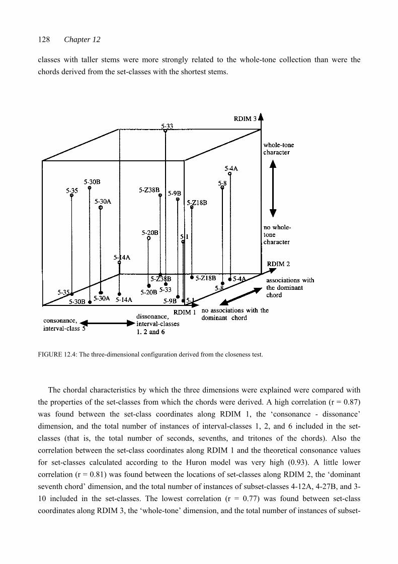
128 Chapter 12
classes with taller stems were more strongly related to the whole-tone collection than were the chords derived from the set-classes with the shortest stems.
FIGURE 12.4: The three-dimensional configuration derived from the closeness test.
The chordal characteristics by which the three dimensions were explained were compared with
the properties of the set-classes from which the chords were derived. A high correlation (r = 0.87) was found between the set-class coordinates along RDIM 1, the ‘consonance - dissonance’ dimension, and the total number of instances of interval-classes 1, 2, and 6 included in the set-classes (that is, the total number of seconds, sevenths, and tritones of the chords). Also the correlation between the set-class coordinates along RDIM 1 and the theoretical consonance values for set-classes calculated according to the Huron model was very high (0.93). A little lower correlation (r = 0.81) was found between the locations of set-classes along RDIM 2, the ‘dominant seventh chord’ dimension, and the total number of instances of subset-classes 4-12A, 4-27B, and 3-10 included in the set-classes. The lowest correlation (r = 0.77) was found between set-class coordinates along RDIM 3, the ‘whole-tone’ dimension, and the total number of instances of subset-
Results I 129
classes of the whole-tone class included in the set-classes. However, all these correlations were high or rather high and statistically very significant (the p-values were .003 or lower).
These correlations indicated that the closeness ratings could be explained by interval-class or subset-class content, but not by them alone. It seemed that the perceived associations with familiar chords and with whole-tone chords could be distracted by ‘extra’ pitches. Each of the test chords had at least one extra pitch added to the dominant seventh chord, and in all but two chords there were pitches not belonging to the whole-tone class. Hence, the chordal setting of the pitches seemed also to influence the ratings, and the results can be said to indicate that the subjects’ closeness ratings were based on both abstract set-class properties and chordal setting. Additionally, the very high correlation between the Huron consonance values and the set-class coordinates validated the consonance model and the analysis simultaneously. 12
12 The importance of the above discussed factors for the subjects’ closeness ratings was tested with yet another method, namely, multiple regression analysis. Seven factors were used as variables in the analysis. These factors were 1) the number of common pitches in pairs; 2) the total number of interval-class 1, 2, and 6 instances in each set-class (this factor seemed to be related to the dissonance of the chords); 3) the total number of interval-class 5 instances in each set-class (this factor was related to the consonance of the chords); 4) the Huron consonance value for each set-class; 5) the total number of subset-class 4-12A, 4-27B, and 3-10 instances in each set-class (this factor seemed to be related to the chords’ association with the dominant chord); 6) the total number of interval-class 2, 4, and 6 instances in each set-class (this factor seemed to be related to the chords’ whole-tone associations), and the total number of interval-class 1 and 5 instances in each set-class. Altogether these variables explained approximately 60 % of the total variance. It was found that the number of common pitches was the most important variable and an independent one. The other important variables were the total number of interval-class 1, 2, and 6 instances (a factor related to RDIM 1) and the total number of subset-class 4-12A, 4-27B, and 3-10 instances (a factor related to RDIM 2). Additionally, large intercorrelations were found between the factors by which RDIM 1 was explained, and, similarly between the factors by which RDIM 3 was explained. Hence, the results of this analysis did not reveal anything new.
CHAPTER THIRTEEN RESULTS II: THE SINGLE-CHORD DATASET
This chapter deals with results analyzed from the single-chord dataset. The data collected in the single-chord test consisted of the subjects’ ratings of 28 chords on nine bipolar semantic scales (see Example 11.2 in Section 11.1 for the scales and translation of the original characteristics). Below, terms ‘single-chord ratings’ or ‘the ratings of chords on scale x’ will be used.
When the subjects’ ratings were scored in Section 11.5, positive signs were given to characteristics on the right side of the scale. The semantic scales were named so that the characteristics with positive signs were given first. Thus, below the scales will be called ‘smooth - rough’, ‘stable - volatile’, ‘dense - sparse’, ‘clear - blurred’, ‘light - gloomy’, ‘round - angular’, ‘colourful - colourless’, ‘lush - barren’, and ‘calm - irritable’.
This chapter is divided into eight sections. In Section 13.1, the subjects’ ratings of each chord on each semantic scale are examined separately. Thereafter, the single-chord dataset is analyzed by three different methods, hierarchical clustering (Section 13.2), factor analysis (Section 13.3), and multidimensional scaling (Section 13.4). The results derived from these analyses are compared in Section 13.5. The results are also compared with the results derived from the multidimensional scaling analysis of the chord-pair dataset. Section 13.6 examines the ratings of some chords on the semantic scales to see how similarly the subjects rated chords derived from the same set-class. In Section 13.7, the single-chord ratings are compared with the similarity values as percentiles calculated by the nine selected similarity measures. Section 13.8 is a summary of Chapter 13.
When the clusters, factors, and dimensions are interpreted, some chordal characteristics are used. Among these characteristics are the total interval contents of the test chords and the series of intervals between adjacent pitches (INT1s); the associations of the test chords with some familiar tonal chords and some familiar chords included as subchords in the test chords; and the width and register of the chords. As in the previous chapter, these chordal characteristics will also be compared with set-class properties, such as the interval-class contents and subset-class contents of
Results II 131
the set-classes from which the chords are derived. For this reason the INT1s and the interval-class vectors will, again, be given in the examples.
Corresponding to the interpretation of the three dimensions analyzed by multidimensional scaling in Section 12.5, correlations between some aspects of the interval-class or subset-class contents of the chords and the locations of the chords along the factors will be calculated in Section 13.3. The locations of the chords are given as the factor scores produced by factor analysis. These correlations will be calculated to confirm the interpretations of the factors.
13.1 UNIFORMITY OF THE SUBJECTS’ RATINGS OF THE CHORDS ON THE NINE SEMANTIC SCALES
Uniformity of the subjects’ ratings of the chords on the semantic scales was examined by two analyses. In the first analysis, each individual subject’s ratings of the chords on each scale were compared with those of all other subjects. This was done to find out how consistently the subjects rated the chords on each scale. In the second analysis, the subjects’ ratings of each chord on each semantic scale were examined separately. These analyses are discussed below.
In the first analysis, correlations were calculated between the ratings of the chords from each subject and the sum of ratings of the chords from all other subjects (hence, 58 correlations were calculated for each scale). The highest and lowest correlations, the number of correlations that were statistically very significant (r ≥ 0.57, p ≤ .001), and the number of correlations that were statistically non-significant (r ≤ 0.37, p ≥ .050) are given in Table 13.1.
As can be seen from the table, the subjects could rate chords consistently on five scales (‘smooth - rough’, ‘stable - volatile’, ‘clear - blurred’, ‘light - gloomy’, and ‘calm - irritable’). The highest correlations were most often between 0.78 and 0.82 (the exception was 0.68 for scale ‘light-gloomy’). Additionally, more than 20 subjects had statistically very significant correlations with other subjects in each of these scales, and only 12 subjects or fewer had non-significant correlations. The scales ‘round - angular’, and ‘lush - barren’, in turn, were not used as consistently as the previous ones by the subjects, even though the highest correlations were still high (0.79 and 0.84 respectively). The number of subjects with statistically very significant correlations with other subjects was 18 or 19, while the number of subjects with non-significant correlations was 19 or 20.
Ratings on the scales ‘dense - sparse’ and ‘colourful - colourless’ seemed to be very problematic. The lowest correlations were -0.37 and -0.63 respectively, and more than 30 subjects (out of 58) had low and non-significant correlations with other subjects. Additionally, only fewer than ten subjects had statistically very significant correlations with others on these scales.
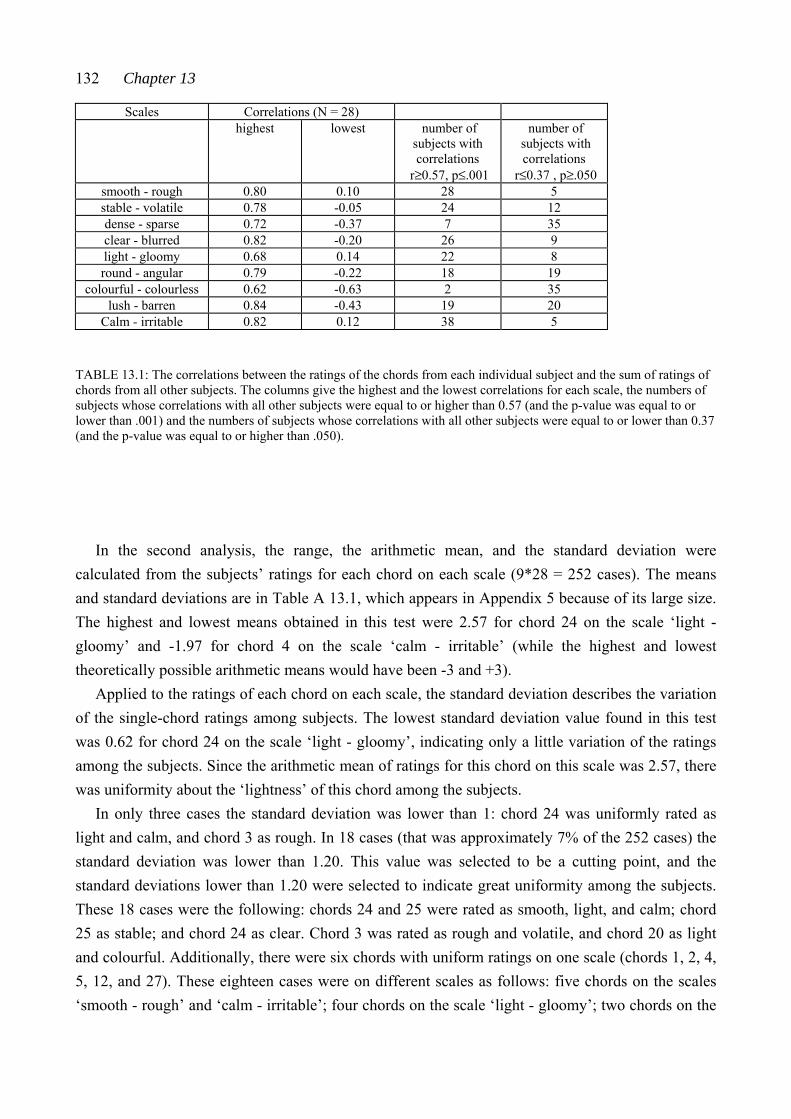
132 Chapter 13
Scales Correlations (N = 28) highest lowest number of
subjects with correlations
r≥0.57, p≤.001
number of subjects with correlations
r≤0.37 , p≥.050 smooth - rough 0.80 0.10 28 5 stable - volatile 0.78 -0.05 24 12 dense - sparse 0.72 -0.37 7 35 clear - blurred 0.82 -0.20 26 9 light - gloomy 0.68 0.14 22 8 round - angular 0.79 -0.22 18 19
colourful - colourless 0.62 -0.63 2 35 lush - barren 0.84 -0.43 19 20
Calm - irritable 0.82 0.12 38 5 TABLE 13.1: The correlations between the ratings of the chords from each individual subject and the sum of ratings of chords from all other subjects. The columns give the highest and the lowest correlations for each scale, the numbers of subjects whose correlations with all other subjects were equal to or higher than 0.57 (and the p-value was equal to or lower than .001) and the numbers of subjects whose correlations with all other subjects were equal to or lower than 0.37 (and the p-value was equal to or higher than .050).
In the second analysis, the range, the arithmetic mean, and the standard deviation were
calculated from the subjects’ ratings for each chord on each scale (9*28 = 252 cases). The means and standard deviations are in Table A 13.1, which appears in Appendix 5 because of its large size. The highest and lowest means obtained in this test were 2.57 for chord 24 on the scale ‘light - gloomy’ and -1.97 for chord 4 on the scale ‘calm - irritable’ (while the highest and lowest theoretically possible arithmetic means would have been -3 and +3).
Applied to the ratings of each chord on each scale, the standard deviation describes the variation of the single-chord ratings among subjects. The lowest standard deviation value found in this test was 0.62 for chord 24 on the scale ‘light - gloomy’, indicating only a little variation of the ratings among the subjects. Since the arithmetic mean of ratings for this chord on this scale was 2.57, there was uniformity about the ‘lightness’ of this chord among the subjects.
In only three cases the standard deviation was lower than 1: chord 24 was uniformly rated as light and calm, and chord 3 as rough. In 18 cases (that was approximately 7% of the 252 cases) the standard deviation was lower than 1.20. This value was selected to be a cutting point, and the standard deviations lower than 1.20 were selected to indicate great uniformity among the subjects. These 18 cases were the following: chords 24 and 25 were rated as smooth, light, and calm; chord 25 as stable; and chord 24 as clear. Chord 3 was rated as rough and volatile, and chord 20 as light and colourful. Additionally, there were six chords with uniform ratings on one scale (chords 1, 2, 4, 5, 12, and 27). These eighteen cases were on different scales as follows: five chords on the scales ‘smooth - rough’ and ‘calm - irritable’; four chords on the scale ‘light - gloomy’; two chords on the
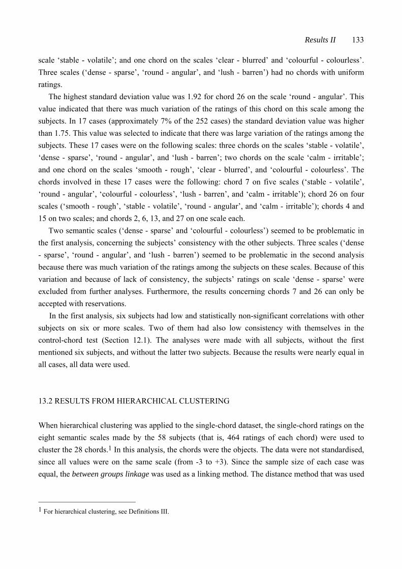
Results II 133
scale ‘stable - volatile’; and one chord on the scales ‘clear - blurred’ and ‘colourful - colourless’. Three scales (‘dense - sparse’, ‘round - angular’, and ‘lush - barren’) had no chords with uniform ratings.
The highest standard deviation value was 1.92 for chord 26 on the scale ‘round - angular’. This value indicated that there was much variation of the ratings of this chord on this scale among the subjects. In 17 cases (approximately 7% of the 252 cases) the standard deviation value was higher than 1.75. This value was selected to indicate that there was large variation of the ratings among the subjects. These 17 cases were on the following scales: three chords on the scales ‘stable - volatile’, ‘dense - sparse’, ‘round - angular’, and ‘lush - barren’; two chords on the scale ‘calm - irritable’; and one chord on the scales ‘smooth - rough’, ‘clear - blurred’, and ‘colourful - colourless’. The chords involved in these 17 cases were the following: chord 7 on five scales (‘stable - volatile’, ‘round - angular’, ‘colourful - colourless’, ‘lush - barren’, and ‘calm - irritable’); chord 26 on four scales (‘smooth - rough’, ‘stable - volatile’, ‘round - angular’, and ‘calm - irritable’); chords 4 and 15 on two scales; and chords 2, 6, 13, and 27 on one scale each.
Two semantic scales (‘dense - sparse’ and ‘colourful - colourless’) seemed to be problematic in the first analysis, concerning the subjects’ consistency with the other subjects. Three scales (‘dense - sparse’, ‘round - angular’, and ‘lush - barren’) seemed to be problematic in the second analysis because there was much variation of the ratings among the subjects on these scales. Because of this variation and because of lack of consistency, the subjects’ ratings on scale ‘dense - sparse’ were excluded from further analyses. Furthermore, the results concerning chords 7 and 26 can only be accepted with reservations.
In the first analysis, six subjects had low and statistically non-significant correlations with other subjects on six or more scales. Two of them had also low consistency with themselves in the control-chord test (Section 12.1). The analyses were made with all subjects, without the first mentioned six subjects, and without the latter two subjects. Because the results were nearly equal in all cases, all data were used.
13.2 RESULTS FROM HIERARCHICAL CLUSTERING
When hierarchical clustering was applied to the single-chord dataset, the single-chord ratings on the eight semantic scales made by the 58 subjects (that is, 464 ratings of each chord) were used to cluster the 28 chords.1 In this analysis, the chords were the objects. The data were not standardised, since all values were on the same scale (from -3 to +3). Since the sample size of each case was equal, the between groups linkage was used as a linking method. The distance method that was used
1 For hierarchical clustering, see Definitions III.
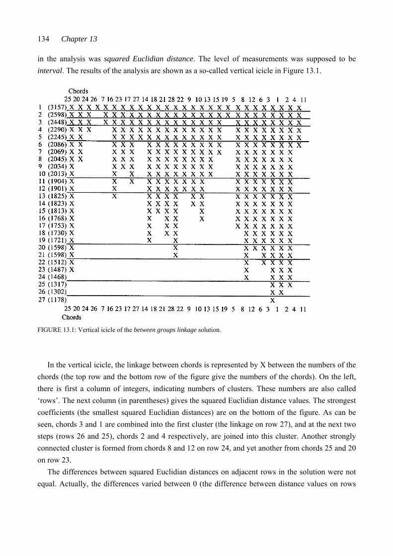
134 Chapter 13
in the analysis was squared Euclidian distance. The level of measurements was supposed to be interval. The results of the analysis are shown as a so-called vertical icicle in Figure 13.1.
FIGURE 13.1: Vertical icicle of the between groups linkage solution.
In the vertical icicle, the linkage between chords is represented by X between the numbers of the
chords (the top row and the bottom row of the figure give the numbers of the chords). On the left, there is first a column of integers, indicating numbers of clusters. These numbers are also called ‘rows’. The next column (in parentheses) gives the squared Euclidian distance values. The strongest coefficients (the smallest squared Euclidian distances) are on the bottom of the figure. As can be seen, chords 3 and 1 are combined into the first cluster (the linkage on row 27), and at the next two steps (rows 26 and 25), chords 2 and 4 respectively, are joined into this cluster. Another strongly connected cluster is formed from chords 8 and 12 on row 24, and yet another from chords 25 and 20 on row 23.
The differences between squared Euclidian distances on adjacent rows in the solution were not equal. Actually, the differences varied between 0 (the difference between distance values on rows
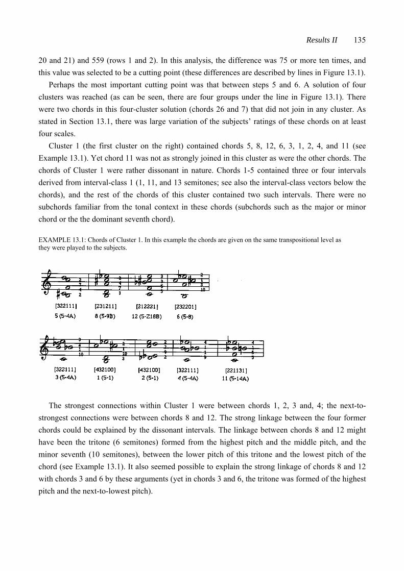
Results II 135
20 and 21) and 559 (rows 1 and 2). In this analysis, the difference was 75 or more ten times, and this value was selected to be a cutting point (these differences are described by lines in Figure 13.1).
Perhaps the most important cutting point was that between steps 5 and 6. A solution of four clusters was reached (as can be seen, there are four groups under the line in Figure 13.1). There were two chords in this four-cluster solution (chords 26 and 7) that did not join in any cluster. As stated in Section 13.1, there was large variation of the subjects’ ratings of these chords on at least four scales.
Cluster 1 (the first cluster on the right) contained chords 5, 8, 12, 6, 3, 1, 2, 4, and 11 (see Example 13.1). Yet chord 11 was not as strongly joined in this cluster as were the other chords. The chords of Cluster 1 were rather dissonant in nature. Chords 1-5 contained three or four intervals derived from interval-class 1 (1, 11, and 13 semitones; see also the interval-class vectors below the chords), and the rest of the chords of this cluster contained two such intervals. There were no subchords familiar from the tonal context in these chords (subchords such as the major or minor chord or the the dominant seventh chord).
EXAMPLE 13.1: Chords of Cluster 1. In this example the chords are given on the same transpositional level as they were played to the subjects.
The strongest connections within Cluster 1 were between chords 1, 2, 3 and, 4; the next-to-strongest connections were between chords 8 and 12. The strong linkage between the four former chords could be explained by the dissonant intervals. The linkage between chords 8 and 12 might have been the tritone (6 semitones) formed from the highest pitch and the middle pitch, and the minor seventh (10 semitones), between the lower pitch of this tritone and the lowest pitch of the chord (see Example 13.1). It also seemed possible to explain the strong linkage of chords 8 and 12 with chords 3 and 6 by these arguments (yet in chords 3 and 6, the tritone was formed of the highest pitch and the next-to-lowest pitch).
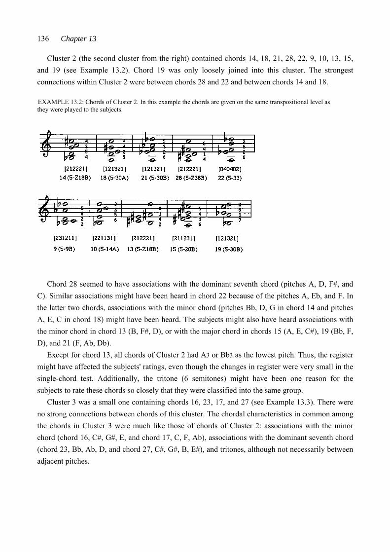
136 Chapter 13
Cluster 2 (the second cluster from the right) contained chords 14, 18, 21, 28, 22, 9, 10, 13, 15, and 19 (see Example 13.2). Chord 19 was only loosely joined into this cluster. The strongest connections within Cluster 2 were between chords 28 and 22 and between chords 14 and 18.
EXAMPLE 13.2: Chords of Cluster 2. In this example the chords are given on the same transpositional level as they were played to the subjects.
Chord 28 seemed to have associations with the dominant seventh chord (pitches A, D, F#, and
C). Similar associations might have been heard in chord 22 because of the pitches A, Eb, and F. In the latter two chords, associations with the minor chord (pitches Bb, D, G in chord 14 and pitches A, E, C in chord 18) might have been heard. The subjects might also have heard associations with the minor chord in chord 13 (B, F#, D), or with the major chord in chords 15 (A, E, C#), 19 (Bb, F, D), and 21 (F, Ab, Db).
Except for chord 13, all chords of Cluster 2 had A3 or Bb3 as the lowest pitch. Thus, the register might have affected the subjects' ratings, even though the changes in register were very small in the single-chord test. Additionally, the tritone (6 semitones) might have been one reason for the subjects to rate these chords so closely that they were classified into the same group.
Cluster 3 was a small one containing chords 16, 23, 17, and 27 (see Example 13.3). There were no strong connections between chords of this cluster. The chordal characteristics in common among the chords in Cluster 3 were much like those of chords of Cluster 2: associations with the minor chord (chord 16, C#, G#, E, and chord 17, C, F, Ab), associations with the dominant seventh chord (chord 23, Bb, Ab, D, and chord 27, C#, G#, B, E#), and tritones, although not necessarily between adjacent pitches.
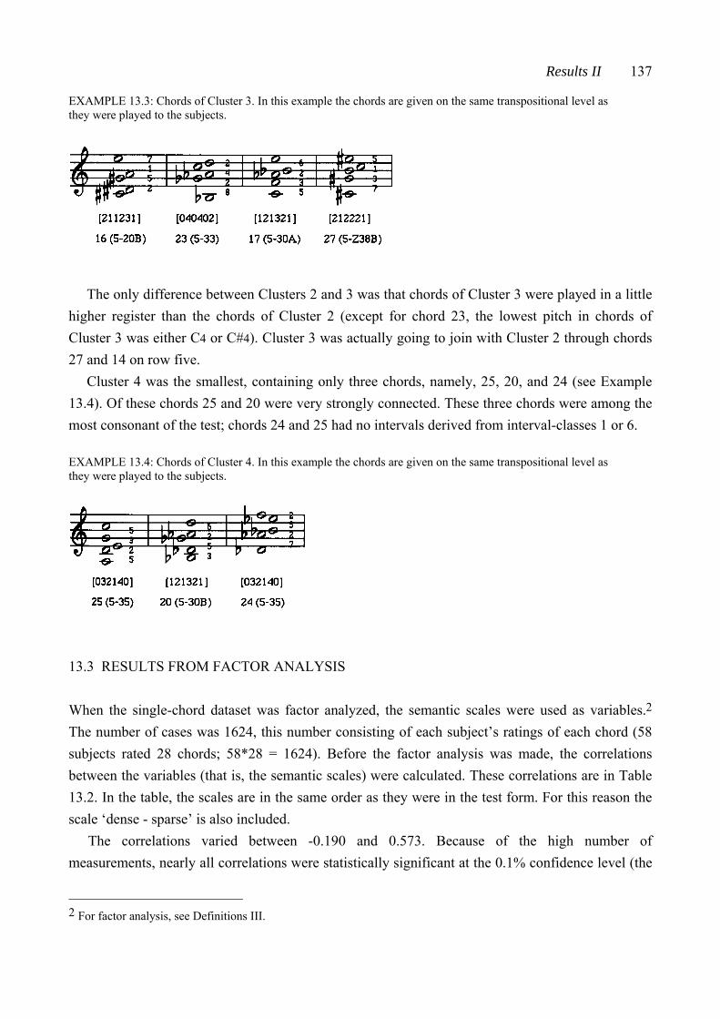
Results II 137
EXAMPLE 13.3: Chords of Cluster 3. In this example the chords are given on the same transpositional level as they were played to the subjects.
The only difference between Clusters 2 and 3 was that chords of Cluster 3 were played in a little higher register than the chords of Cluster 2 (except for chord 23, the lowest pitch in chords of Cluster 3 was either C4 or C#4). Cluster 3 was actually going to join with Cluster 2 through chords 27 and 14 on row five.
Cluster 4 was the smallest, containing only three chords, namely, 25, 20, and 24 (see Example 13.4). Of these chords 25 and 20 were very strongly connected. These three chords were among the most consonant of the test; chords 24 and 25 had no intervals derived from interval-classes 1 or 6.
EXAMPLE 13.4: Chords of Cluster 4. In this example the chords are given on the same transpositional level as they were played to the subjects.
13.3 RESULTS FROM FACTOR ANALYSIS
When the single-chord dataset was factor analyzed, the semantic scales were used as variables.2 The number of cases was 1624, this number consisting of each subject’s ratings of each chord (58 subjects rated 28 chords; 58*28 = 1624). Before the factor analysis was made, the correlations between the variables (that is, the semantic scales) were calculated. These correlations are in Table 13.2. In the table, the scales are in the same order as they were in the test form. For this reason the scale ‘dense - sparse’ is also included.
The correlations varied between -0.190 and 0.573. Because of the high number of measurements, nearly all correlations were statistically significant at the 0.1% confidence level (the
2 For factor analysis, see Definitions III.
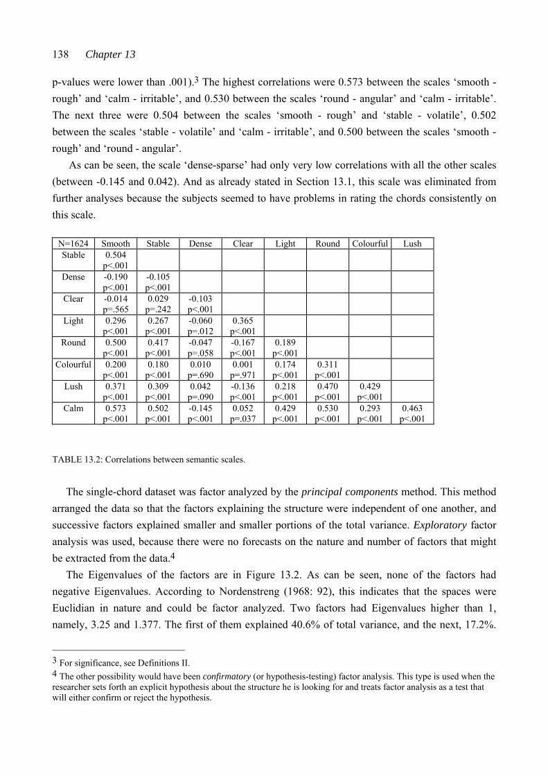
138 Chapter 13
p-values were lower than .001).3 The highest correlations were 0.573 between the scales ‘smooth - rough’ and ‘calm - irritable’, and 0.530 between the scales ‘round - angular’ and ‘calm - irritable’. The next three were 0.504 between the scales ‘smooth - rough’ and ‘stable - volatile’, 0.502 between the scales ‘stable - volatile’ and ‘calm - irritable’, and 0.500 between the scales ‘smooth - rough’ and ‘round - angular’.
As can be seen, the scale ‘dense-sparse’ had only very low correlations with all the other scales (between -0.145 and 0.042). And as already stated in Section 13.1, this scale was eliminated from further analyses because the subjects seemed to have problems in rating the chords consistently on this scale.
N=1624 Smooth Stable Dense Clear Light Round Colourful Lush Stable 0.504
p<.001
Dense -0.190 p<.001
-0.105 p<.001
Clear -0.014 p=.565
0.029 p=.242
-0.103 p<.001
Light 0.296 p<.001
0.267 p<.001
-0.060 p=.012
0.365 p<.001
Round 0.500 p<.001
0.417 p<.001
-0.047 p=.058
-0.167 p<.001
0.189 p<.001
Colourful 0.200 p<.001
0.180 p<.001
0.010 p=.690
0.001 p=.971
0.174 p<.001
0.311 p<.001
Lush 0.371 p<.001
0.309 p<.001
0.042 p=.090
-0.136 p<.001
0.218 p<.001
0.470 p<.001
0.429 p<.001
Calm 0.573 p<.001
0.502 p<.001
-0.145 p<.001
0.052 p=.037
0.429 p<.001
0.530 p<.001
0.293 p<.001
0.463 p<.001
TABLE 13.2: Correlations between semantic scales. The single-chord dataset was factor analyzed by the principal components method. This method
arranged the data so that the factors explaining the structure were independent of one another, and successive factors explained smaller and smaller portions of the total variance. Exploratory factor analysis was used, because there were no forecasts on the nature and number of factors that might be extracted from the data.4
The Eigenvalues of the factors are in Figure 13.2. As can be seen, none of the factors had negative Eigenvalues. According to Nordenstreng (1968: 92), this indicates that the spaces were Euclidian in nature and could be factor analyzed. Two factors had Eigenvalues higher than 1, namely, 3.25 and 1.377. The first of them explained 40.6% of total variance, and the next, 17.2%.
3 For significance, see Definitions II. 4 The other possibility would have been confirmatory (or hypothesis-testing) factor analysis. This type is used when the researcher sets forth an explicit hypothesis about the structure he is looking for and treats factor analysis as a test that will either confirm or reject the hypothesis.
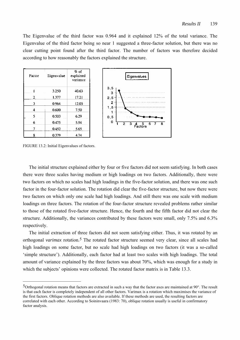
Results II 139
The Eigenvalue of the third factor was 0.964 and it explained 12% of the total variance. The Eigenvalue of the third factor being so near 1 suggested a three-factor solution, but there was no clear cutting point found after the third factor. The number of factors was therefore decided according to how reasonably the factors explained the structure.
FIGURE 13.2: Initial Eigenvalues of factors.
The initial structure explained either by four or five factors did not seem satisfying. In both cases
there were three scales having medium or high loadings on two factors. Additionally, there were two factors on which no scales had high loadings in the five-factor solution, and there was one such factor in the four-factor solution. The rotation did clear the five-factor structure, but now there were two factors on which only one scale had high loadings. And still there was one scale with medium loadings on three factors. The rotation of the four-factor structure revealed problems rather similar to those of the rotated five-factor structure. Hence, the fourth and the fifth factor did not clear the structure. Additionally, the variances contributed by these factors were small, only 7.5% and 6.3% respectively.
The initial extraction of three factors did not seem satisfying either. Thus, it was rotated by an orthogonal varimax rotation.5 The rotated factor structure seemed very clear, since all scales had high loadings on some factor, but no scale had high loadings on two factors (it was a so-called ‘simple structure’). Additionally, each factor had at least two scales with high loadings. The total amount of variance explained by the three factors was about 70%, which was enough for a study in which the subjects’ opinions were collected. The rotated factor matrix is in Table 13.3. 5Orthogonal rotation means that factors are extracted in such a way that the factor axes are maintained at 90°. The result is that each factor is completely independent of all other factors. Varimax is a rotation which maximises the variance of the first factors. Oblique rotation methods are also available. If these methods are used, the resulting factors are correlated with each other. According to Soininvaara (1983: 70), oblique rotation usually is useful in confirmatory factor analysis.
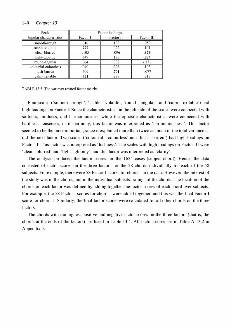
140 Chapter 13
Scale Factor loadings bipolar characteristics Factor I Factor II Factor III
smooth-rough .816 .103 .059 stable-volatile .777 .022 .101 clear-blurred -.105 -.096 .876 light-gloomy .349 .176 .734 round-angular .684 .382 -.171
colourful-colourless .040 .893 .103 lush-barren .409 .701 -.077
calm-irritable .751 .299 .217 TABLE 13.3: The varimax rotated factor matrix.
Four scales (‘smooth - rough’, ‘stable - volatile’, ‘round - angular’, and ‘calm - irritable’) had
high loadings on Factor I. Since the characteristics on the left side of the scales were connected with softness, mildness, and harmoniousness while the opposite characteristics were connected with hardness, tenseness, or disharmony, this factor was interpreted as ‘harmoniousness’. This factor seemed to be the most important, since it explained more than twice as much of the total variance as did the next factor. Two scales (‘colourful - colourless’ and ‘lush - barren’) had high loadings on Factor II. This factor was interpreted as ‘lushness’. The scales with high loadings on Factor III were ‘clear - blurred’ and ‘light - gloomy’, and this factor was interpreted as ‘clarity’.
The analysis produced the factor scores for the 1624 cases (subject-chord). Hence, the data consisted of factor scores on the three factors for the 28 chords individually for each of the 58 subjects. For example, there were 58 Factor I scores for chord 1 in the data. However, the interest of the study was in the chords, not in the individual subjects’ ratings of the chords. The location of the chords on each factor was defined by adding together the factor scores of each chord over subjects. For example, the 58 Factor I scores for chord 1 were added together, and this was the final Factor I score for chord 1. Similarly, the final factor scores were calculated for all other chords on the three factors.
The chords with the highest positive and negative factor scores on the three factors (that is, the chords at the ends of the factors) are listed in Table 13.4. All factor scores are in Table A 13.2 in Appendix 5.
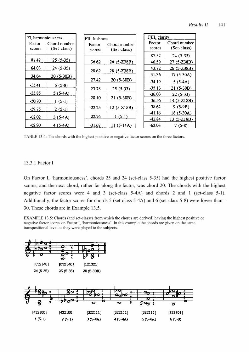
Results II 141
TABLE 13.4: The chords with the highest positive or negative factor scores on the three factors.
13.3.1 Factor I
On Factor I, ‘harmoniousness’, chords 25 and 24 (set-class 5-35) had the highest positive factor scores, and the next chord, rather far along the factor, was chord 20. The chords with the highest negative factor scores were 4 and 3 (set-class 5-4A) and chords 2 and 1 (set-class 5-1). Additionally, the factor scores for chords 5 (set-class 5-4A) and 6 (set-class 5-8) were lower than -30. These chords are in Example 13.5. EXAMPLE 13.5: Chords (and set-classes from which the chords are derived) having the highest positive or negative factor scores on Factor I, ‘harmoniousness’. In this example the chords are given on the same transpositional level as they were played to the subjects.
142 Chapter 13
The six chords with the highest negative factor scores had dissonant intervals derived from interval-class 1: 1, 11, or 13 semitones. Chords 3, 4, and 5 also included a tritone (6 semitones, interval-class 6). Chords 24 and 25 of the opposite end of this factor had no such intervals; instead they had relatively many perfect fourths and fifths (5 or 7 semitones; see INT1s and interval-class vectors in Example 13.5).
To examine further the connection between Factor I and set-class properties, correlations were calculated between the locations of the chords on this factor and the interval-class contents of the chords. The correlation between the factor scores of the 28 chords on Factor I and the total number of intervals derived from interval-class 1 within each chord was high (r = -0.81, p < .001). The correlation between factor scores and the total number of intervals derived from interval-classes 1 and 6 was still higher (r = -0.85, p < .001). These correlations were negative, since the chords with the highest negative factor scores had the highest number of intervals derived from the mentioned interval-classes. The correlation between factor scores and the total number of intervals derived from interval-class 5 was lower, but statistically very significant (r = 0.63, p < .001).6
These correlations indicated that there was a connection between factor scores on Factor I and the interval-class contents of the chords. Since the interval-class content of a chord is also a property of the set-class from which the chord is derived, these correlations could be interpreted to indicate a connection between set-classes and the subjects’ ratings of the chords as well.
Because of the qualities of the semantic scales with high loadings on Factor I and because of the interval contents of the chords with the highest factor scores, this factor seemed to be connected to the degree of consonance of the test chords. To further examine this connection, the factor scores of the chords were compared with the theoretical consonance values for the chords calculated by two models, namely, the Malmberg (1918) model and the Kameoka and Kuriyagawa (1969) model (see Sections 5.2 and 10.2 for the models and Table 10.1 for the values).
The correlation between the factor scores of the chords on Factor I and the Malmberg values for the chords was high (r = 0.81, p < .001). The correlation for the Kameoka and Kuriyagawa values was lower (r = -0.70, p < .001). Both correlations were statistically very significant, and they indicated a connection between theoretical consonance and location of chords on Factor I. The correlation for the Malmberg model was positive, since this model measured consonance, and the correlation for the Kameoka and Kuriyagawa model was negative, since this model measured dissonance. As mentioned earlier, the positive factor scores indicated harmoniousness.7
6 Correlations between factor scores of the chords on each factor and certain aspects of the interval-class contents of the chords are in Table A 13.3 in Appendix 5. 7 Correlations between factor scores of the 28 chords on each factor and certain chordal characteristics are in Table A 13.4 in Appendix 5.
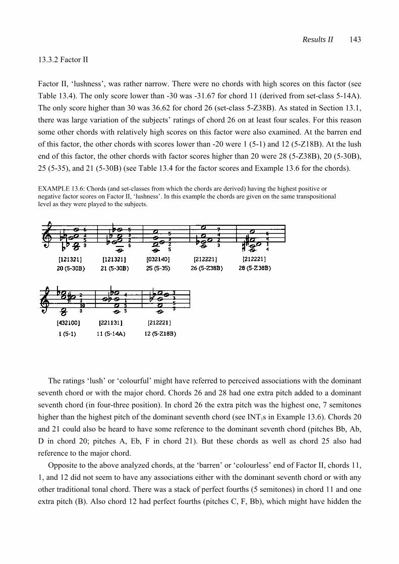
Results II 143
13.3.2 Factor II
Factor II, ‘lushness’, was rather narrow. There were no chords with high scores on this factor (see Table 13.4). The only score lower than -30 was -31.67 for chord 11 (derived from set-class 5-14A). The only score higher than 30 was 36.62 for chord 26 (set-class 5-Z38B). As stated in Section 13.1, there was large variation of the subjects’ ratings of chord 26 on at least four scales. For this reason some other chords with relatively high scores on this factor were also examined. At the barren end of this factor, the other chords with scores lower than -20 were 1 (5-1) and 12 (5-Z18B). At the lush end of this factor, the other chords with factor scores higher than 20 were 28 (5-Z38B), 20 (5-30B), 25 (5-35), and 21 (5-30B) (see Table 13.4 for the factor scores and Example 13.6 for the chords).
EXAMPLE 13.6: Chords (and set-classes from which the chords are derived) having the highest positive or negative factor scores on Factor II, ‘lushness’. In this example the chords are given on the same transpositional level as they were played to the subjects.
The ratings ‘lush’ or ‘colourful’ might have referred to perceived associations with the dominant
seventh chord or with the major chord. Chords 26 and 28 had one extra pitch added to a dominant seventh chord (in four-three position). In chord 26 the extra pitch was the highest one, 7 semitones higher than the highest pitch of the dominant seventh chord (see INT1s in Example 13.6). Chords 20 and 21 could also be heard to have some reference to the dominant seventh chord (pitches Bb, Ab, D in chord 20; pitches A, Eb, F in chord 21). But these chords as well as chord 25 also had reference to the major chord.
Opposite to the above analyzed chords, at the ‘barren’ or ‘colourless’ end of Factor II, chords 11, 1, and 12 did not seem to have any associations either with the dominant seventh chord or with any other traditional tonal chord. There was a stack of perfect fourths (5 semitones) in chord 11 and one extra pitch (B). Also chord 12 had perfect fourths (pitches C, F, Bb), which might have hidden the
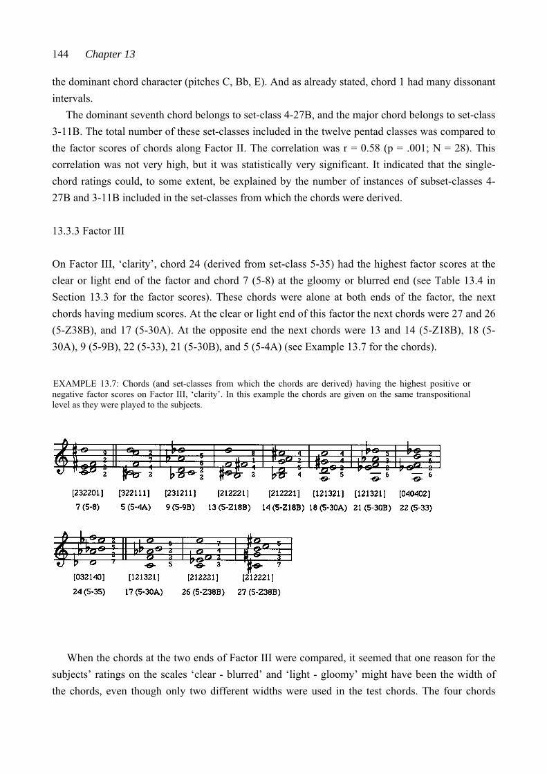
144 Chapter 13
the dominant chord character (pitches C, Bb, E). And as already stated, chord 1 had many dissonant intervals.
The dominant seventh chord belongs to set-class 4-27B, and the major chord belongs to set-class 3-11B. The total number of these set-classes included in the twelve pentad classes was compared to the factor scores of chords along Factor II. The correlation was r = 0.58 (p = .001; N = 28). This correlation was not very high, but it was statistically very significant. It indicated that the single-chord ratings could, to some extent, be explained by the number of instances of subset-classes 4-27B and 3-11B included in the set-classes from which the chords were derived.
13.3.3 Factor III
On Factor III, ‘clarity’, chord 24 (derived from set-class 5-35) had the highest factor scores at the clear or light end of the factor and chord 7 (5-8) at the gloomy or blurred end (see Table 13.4 in Section 13.3 for the factor scores). These chords were alone at both ends of the factor, the next chords having medium scores. At the clear or light end of this factor the next chords were 27 and 26 (5-Z38B), and 17 (5-30A). At the opposite end the next chords were 13 and 14 (5-Z18B), 18 (5-30A), 9 (5-9B), 22 (5-33), 21 (5-30B), and 5 (5-4A) (see Example 13.7 for the chords). EXAMPLE 13.7: Chords (and set-classes from which the chords are derived) having the highest positive or negative factor scores on Factor III, ‘clarity’. In this example the chords are given on the same transpositional level as they were played to the subjects.
When the chords at the two ends of Factor III were compared, it seemed that one reason for the
subjects’ ratings on the scales ‘clear - blurred’ and ‘light - gloomy’ might have been the width of the chords, even though only two different widths were used in the test chords. The four chords

Results II 145
with the highest positive factor scores (chords 24, 27, 26, and 17) had the width of 16 semitones. In addition, the next two chords along this factor (chords 8 and 3) were of the same width. At the opposite end of Factor III, the width of most chords was 15 semitones (chords 7, 5, 9, 13, 14, and 18). To examine this connection further, the correlation between factor scores of the chords on Factor III and the width of the chords was calculated. It was medium (r = 0.43; see Table A 13.4 in Appendix 5), but it was statistically significant (p = .017). This correlation suggested that the width had some effect on perception of chords.
The register of the chords seemed also to have affected to the single-chord ratings, even though the variation in register was small in the single-chord test. In the four chords that had the highest scores on Factor III, ‘clarity’, the lowest pitch was C4 twice and C#4 twice. In the chords with high negative scores on this factor the lowest pitch was A3 three times, Bb3 twice, and B3 twice. The correlation between the lowest pitch of each chord and the factor scores of the chords on Factor III indicated a rather high connection (r = 0.60, p = .001).8 But the combined effect of the lowest pitch and the width of each chord was found to be the most forceful explanation of the factor scores along the third factor. The correlation between the Factor III scores and the combined effect of the lowest pitch and the width of the chords was rather high and statistically very significant (r = 0.74, p < .001).9 13.3.4 Abstract of Sections 13.3.1 - 13.3.3
The factor analyzed solution from the single-chord dataset was clear and interpretable. Figure 13.3 gives the picture of the three-factor solution. This figure also gives the chordal characteristics by which the factors were explained. The white dots stand for the 16-semitone chords, and the black dots stand for the 15-semitone chords.
The chords near the right side were the most consonant used in the test, and the chords near the left side were dissonant. The chords near the front wall did not have associations with any familiar chord, while the chords near the back wall seemed to have reference to the dominant seventh chord or to the major chord. The chords with higher stems were generally played in a higher register and had the width of 16 semitones, while the chords with the shorter stems usually had the width of 15 semitones and were played in a lower register.
8 When this correlation was calculated, the lowest pitch of each chord was represented by numeric value: value 1 was assigned to A3, value 2 to Bb3, value 3 to B3, value 4 to C4, and value 5 to C#4. 9 The combined effect of the lowest pitch and the width was calculated in the following way: value 2 represented the width of 16 semitones and value 0 the width of 15 semitones. The value representing the width of each chord was added to the value representing the lowest pitch of the chord.
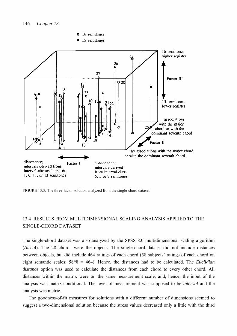
146 Chapter 13
FIGURE 13.3: The three-factor solution analyzed from the single-chord dataset.
13.4 RESULTS FROM MULTIDIMENSIONAL SCALING ANALYSIS APPLIED TO THE SINGLE-CHORD DATASET
The single-chord dataset was also analyzed by the SPSS 8.0 multidimensional scaling algorithm (Alscal). The 28 chords were the objects. The single-chord dataset did not include distances between objects, but did include 464 ratings of each chord (58 subjects’ ratings of each chord on eight semantic scales; 58*8 = 464). Hence, the distances had to be calculated. The Euclidian distance option was used to calculate the distances from each chord to every other chord. All distances within the matrix were on the same measurement scale, and, hence, the input of the analysis was matrix-conditional. The level of measurement was supposed to be interval and the analysis was metric.
The goodness-of-fit measures for solutions with a different number of dimensions seemed to suggest a two-dimensional solution because the stress values decreased only a little with the third
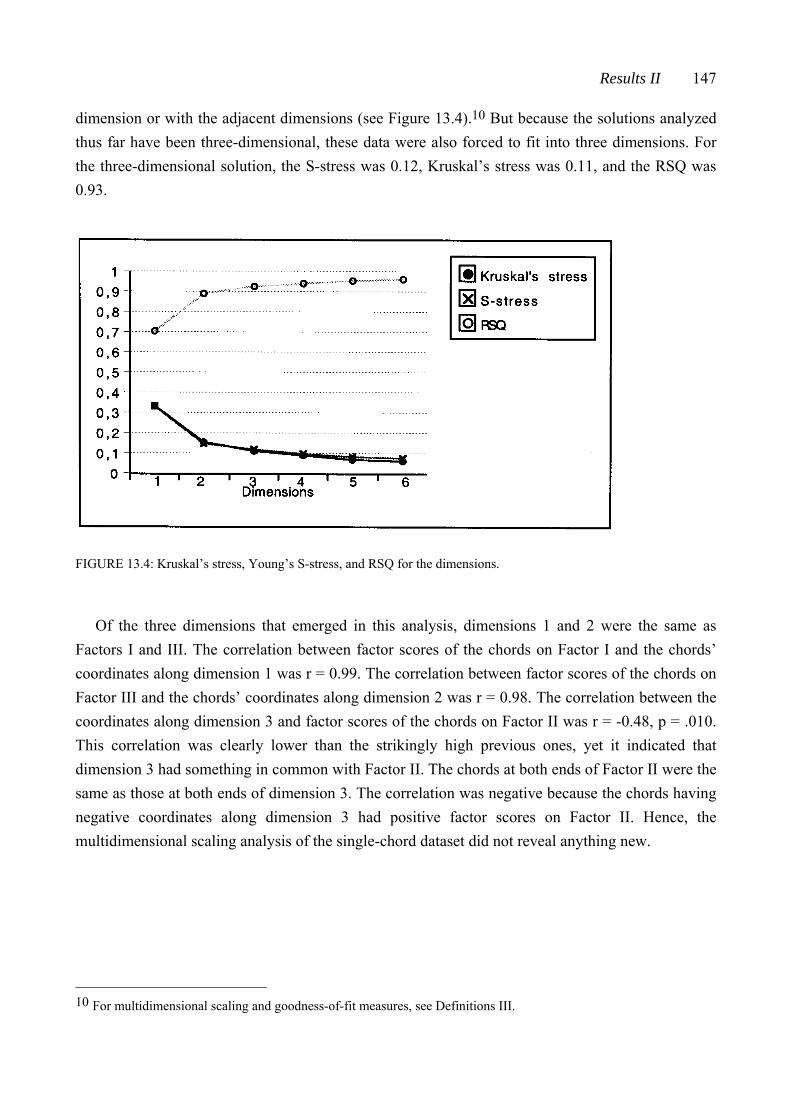
Results II 147
dimension or with the adjacent dimensions (see Figure 13.4).10 But because the solutions analyzed thus far have been three-dimensional, these data were also forced to fit into three dimensions. For the three-dimensional solution, the S-stress was 0.12, Kruskal’s stress was 0.11, and the RSQ was 0.93.
FIGURE 13.4: Kruskal’s stress, Young’s S-stress, and RSQ for the dimensions.
Of the three dimensions that emerged in this analysis, dimensions 1 and 2 were the same as Factors I and III. The correlation between factor scores of the chords on Factor I and the chords’ coordinates along dimension 1 was r = 0.99. The correlation between factor scores of the chords on Factor III and the chords’ coordinates along dimension 2 was r = 0.98. The correlation between the coordinates along dimension 3 and factor scores of the chords on Factor II was r = -0.48, p = .010. This correlation was clearly lower than the strikingly high previous ones, yet it indicated that dimension 3 had something in common with Factor II. The chords at both ends of Factor II were the same as those at both ends of dimension 3. The correlation was negative because the chords having negative coordinates along dimension 3 had positive factor scores on Factor II. Hence, the multidimensional scaling analysis of the single-chord dataset did not reveal anything new.
10 For multidimensional scaling and goodness-of-fit measures, see Definitions III.
148 Chapter 13
13.5 COMPARISON OF RESULTS ANALYZED FROM THE CHORD-PAIR DATASET AND THE SINGLE-CHORD DATASET
There seemed to be a clear connection between the Factor I and Clusters 1 and 4. The same chords were in Cluster 1 and at the dissonant end of Factor I, while the chords of Cluster 4 were at the harmonious end of Factor I. Additionally, the chords at the ends of RDIM 1 analyzed from the chord-pair dataset were the same as those at the ends of Factor I and in Clusters 1 and 4 (see Section 12.5.1 for RDIM 1). A high and statistically very significant correlation (r = -0.82, p < .001) was found between factor scores of chords along Factor I and coordinates for set-classes along RDIM 1.11 The correlation was negative because the chords with positive factor scores had negative coordinates on RDIM 1.
The high correlation between Factor I and RDIM 1 indicated that the most important factor guiding the subjects’ ratings was the same for both the single chords and the chord pairs. This finding was supported by the results of the cluster analysis. According to the chords on RDIM 1, on Factor I, and in Clusters 1 and 4, and according to the characteristics of the scales with high loadings on Factor I, this most important factor was interpreted as the degree of consonance of chords.
Some connection was found between RDIM 2 and Factor II (for RDIM 2, see Section 12.5.2). Some of the chords with the highest positive factor scores were derived from the set-classes with high positive coordinates on RDIM 2. These chords were interpreted to have associations with the dominant seventh chord. The associations with some familiar tonal chords were one explanatory factor for Clusters 2 and 3 as well. But the chords with the highest negative factor scores were not derived from the set-classes with high negative coordinates on RDIM 2. Hence, the correlation between the chords’ locations on RDIM 2 and Factor II was very low (r = 0.14).
At the ‘gloomy’ or ‘blurred’ end of Factor III, rather many chords were the same as in Cluster 3. The register of the chords seemed to be the characteristic separating Clusters 2 and 3. The register together with the width of the chords also seemed to be important when Factor III was explained. But there was no other connection between Factor III and Clusters 2 and 3. In the chord-pair test, the width and register of the two chords of each pair were the same, hence, these chordal characteristics could not emerge as an explanatory dimension of the chord-pair dataset. For this reason there could not be any connection between RDIM 3, Factor III, and Clusters 2 and 3.
11 As already stated, the number of set-classes was twelve; hence there were twelve coordinates on RDIM 1. The number of chords, however, was 28, and that was the number of factor scores on Factor I as well. When the correlation between set-class coordinates and factor scores was calculated, the coordinates for the twelve set-classes were taken as coordinates for the 28 chords (the two or three chords derived from the same set-class had the same coordinates). Hence, N was 28 in both sets of measurements.
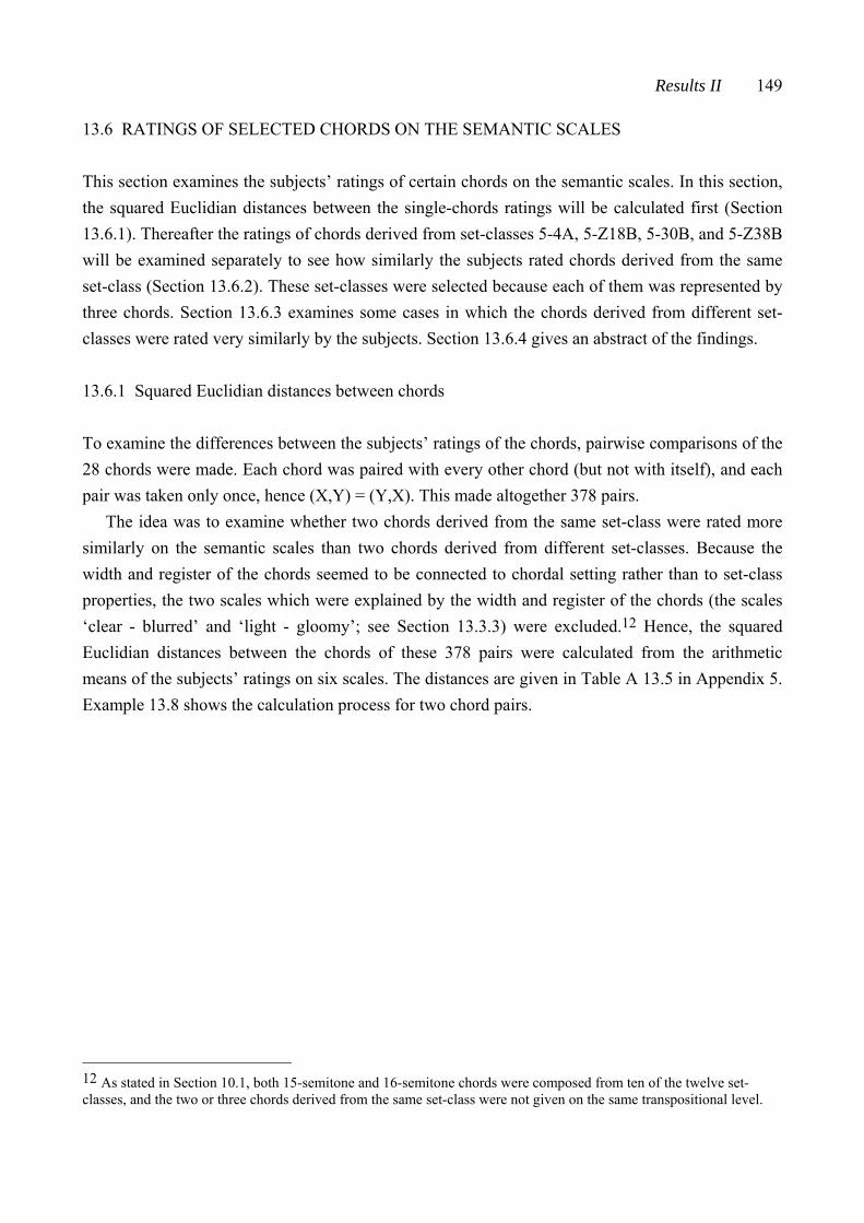
Results II 149
13.6 RATINGS OF SELECTED CHORDS ON THE SEMANTIC SCALES
This section examines the subjects’ ratings of certain chords on the semantic scales. In this section, the squared Euclidian distances between the single-chords ratings will be calculated first (Section 13.6.1). Thereafter the ratings of chords derived from set-classes 5-4A, 5-Z18B, 5-30B, and 5-Z38B will be examined separately to see how similarly the subjects rated chords derived from the same set-class (Section 13.6.2). These set-classes were selected because each of them was represented by three chords. Section 13.6.3 examines some cases in which the chords derived from different set-classes were rated very similarly by the subjects. Section 13.6.4 gives an abstract of the findings. 13.6.1 Squared Euclidian distances between chords
To examine the differences between the subjects’ ratings of the chords, pairwise comparisons of the 28 chords were made. Each chord was paired with every other chord (but not with itself), and each pair was taken only once, hence (X,Y) = (Y,X). This made altogether 378 pairs.
The idea was to examine whether two chords derived from the same set-class were rated more similarly on the semantic scales than two chords derived from different set-classes. Because the width and register of the chords seemed to be connected to chordal setting rather than to set-class properties, the two scales which were explained by the width and register of the chords (the scales ‘clear - blurred’ and ‘light - gloomy’; see Section 13.3.3) were excluded.12 Hence, the squared Euclidian distances between the chords of these 378 pairs were calculated from the arithmetic means of the subjects’ ratings on six scales. The distances are given in Table A 13.5 in Appendix 5. Example 13.8 shows the calculation process for two chord pairs.
12 As stated in Section 10.1, both 15-semitone and 16-semitone chords were composed from ten of the twelve set-classes, and the two or three chords derived from the same set-class were not given on the same transpositional level.
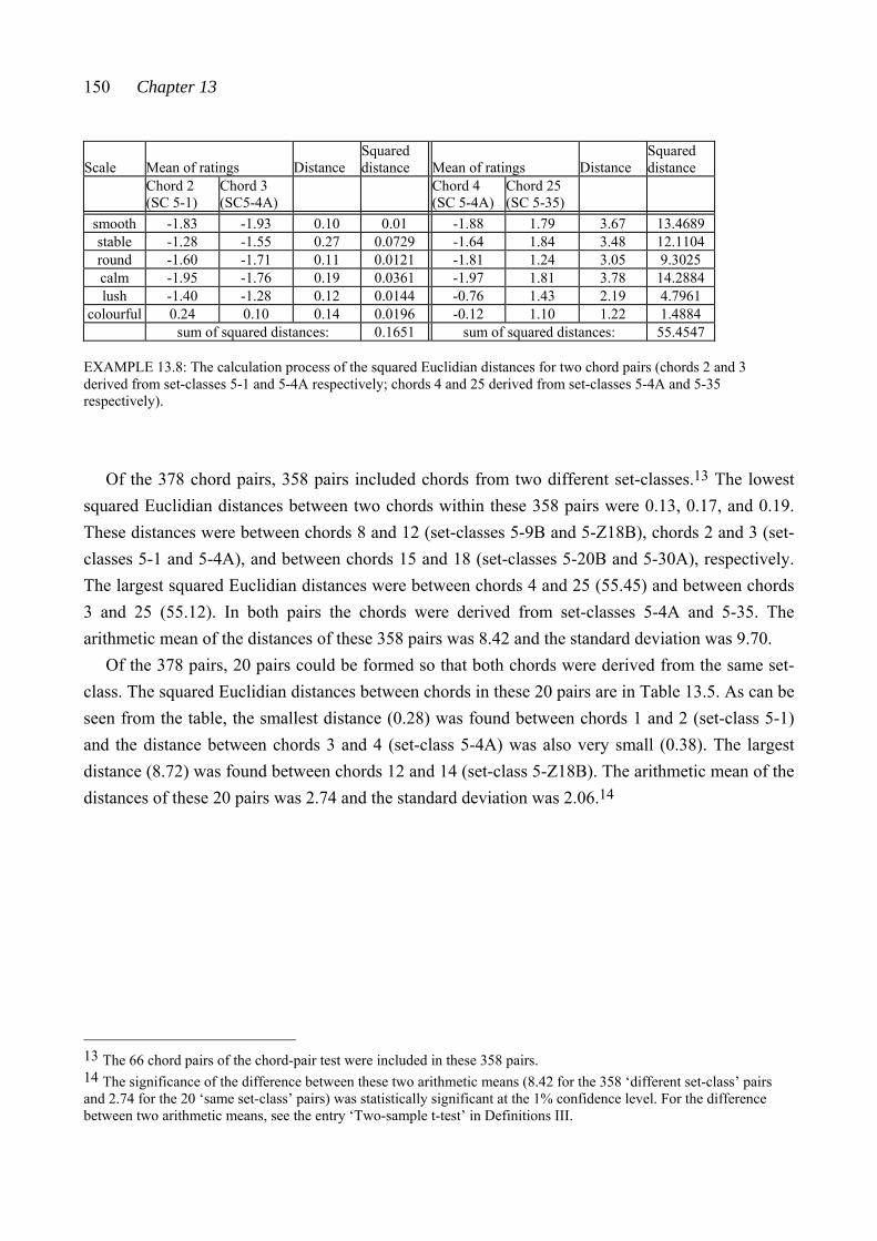
150 Chapter 13
Scale Mean of ratings Distance Squared distance Mean of ratings Distance
Squared distance
Chord 2 (SC 5-1)
Chord 3 (SC5-4A)
Chord 4 (SC 5-4A)
Chord 25 (SC 5-35)
smooth -1.83 -1.93 0.10 0.01 -1.88 1.79 3.67 13.4689 stable -1.28 -1.55 0.27 0.0729 -1.64 1.84 3.48 12.1104 round -1.60 -1.71 0.11 0.0121 -1.81 1.24 3.05 9.3025 calm -1.95 -1.76 0.19 0.0361 -1.97 1.81 3.78 14.2884 lush -1.40 -1.28 0.12 0.0144 -0.76 1.43 2.19 4.7961
colourful 0.24 0.10 0.14 0.0196 -0.12 1.10 1.22 1.4884 sum of squared distances: 0.1651 sum of squared distances: 55.4547
EXAMPLE 13.8: The calculation process of the squared Euclidian distances for two chord pairs (chords 2 and 3 derived from set-classes 5-1 and 5-4A respectively; chords 4 and 25 derived from set-classes 5-4A and 5-35 respectively).
Of the 378 chord pairs, 358 pairs included chords from two different set-classes.13 The lowest
squared Euclidian distances between two chords within these 358 pairs were 0.13, 0.17, and 0.19. These distances were between chords 8 and 12 (set-classes 5-9B and 5-Z18B), chords 2 and 3 (set-classes 5-1 and 5-4A), and between chords 15 and 18 (set-classes 5-20B and 5-30A), respectively. The largest squared Euclidian distances were between chords 4 and 25 (55.45) and between chords 3 and 25 (55.12). In both pairs the chords were derived from set-classes 5-4A and 5-35. The arithmetic mean of the distances of these 358 pairs was 8.42 and the standard deviation was 9.70.
Of the 378 pairs, 20 pairs could be formed so that both chords were derived from the same set-class. The squared Euclidian distances between chords in these 20 pairs are in Table 13.5. As can be seen from the table, the smallest distance (0.28) was found between chords 1 and 2 (set-class 5-1) and the distance between chords 3 and 4 (set-class 5-4A) was also very small (0.38). The largest distance (8.72) was found between chords 12 and 14 (set-class 5-Z18B). The arithmetic mean of the distances of these 20 pairs was 2.74 and the standard deviation was 2.06.14
13 The 66 chord pairs of the chord-pair test were included in these 358 pairs. 14 The significance of the difference between these two arithmetic means (8.42 for the 358 ‘different set-class’ pairs and 2.74 for the 20 ‘same set-class’ pairs) was statistically significant at the 1% confidence level. For the difference between two arithmetic means, see the entry ‘Two-sample t-test’ in Definitions III.
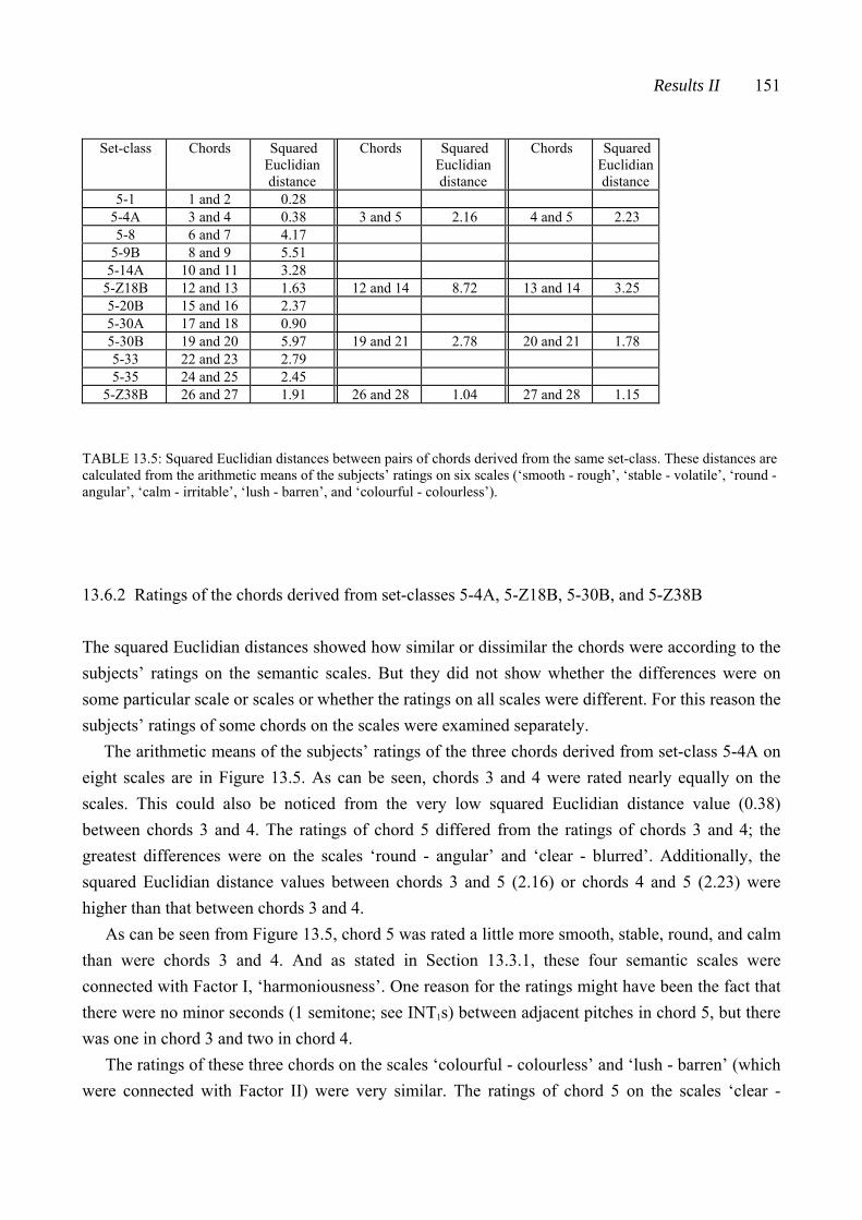
Results II 151
Set-class Chords Squared
Euclidian distance
Chords Squared Euclidian distance
Chords Squared Euclidian distance
5-1 1 and 2 0.28 5-4A 3 and 4 0.38 3 and 5 2.16 4 and 5 2.23 5-8 6 and 7 4.17
5-9B 8 and 9 5.51 5-14A 10 and 11 3.28
5-Z18B 12 and 13 1.63 12 and 14 8.72 13 and 14 3.25 5-20B 15 and 16 2.37 5-30A 17 and 18 0.90 5-30B 19 and 20 5.97 19 and 21 2.78 20 and 21 1.78 5-33 22 and 23 2.79 5-35 24 and 25 2.45
5-Z38B 26 and 27 1.91 26 and 28 1.04 27 and 28 1.15 TABLE 13.5: Squared Euclidian distances between pairs of chords derived from the same set-class. These distances are calculated from the arithmetic means of the subjects’ ratings on six scales (‘smooth - rough’, ‘stable - volatile’, ‘round - angular’, ‘calm - irritable’, ‘lush - barren’, and ‘colourful - colourless’).
13.6.2 Ratings of the chords derived from set-classes 5-4A, 5-Z18B, 5-30B, and 5-Z38B
The squared Euclidian distances showed how similar or dissimilar the chords were according to the subjects’ ratings on the semantic scales. But they did not show whether the differences were on some particular scale or scales or whether the ratings on all scales were different. For this reason the subjects’ ratings of some chords on the scales were examined separately.
The arithmetic means of the subjects’ ratings of the three chords derived from set-class 5-4A on eight scales are in Figure 13.5. As can be seen, chords 3 and 4 were rated nearly equally on the scales. This could also be noticed from the very low squared Euclidian distance value (0.38) between chords 3 and 4. The ratings of chord 5 differed from the ratings of chords 3 and 4; the greatest differences were on the scales ‘round - angular’ and ‘clear - blurred’. Additionally, the squared Euclidian distance values between chords 3 and 5 (2.16) or chords 4 and 5 (2.23) were higher than that between chords 3 and 4.
As can be seen from Figure 13.5, chord 5 was rated a little more smooth, stable, round, and calm than were chords 3 and 4. And as stated in Section 13.3.1, these four semantic scales were connected with Factor I, ‘harmoniousness’. One reason for the ratings might have been the fact that there were no minor seconds (1 semitone; see INT1s) between adjacent pitches in chord 5, but there was one in chord 3 and two in chord 4.
The ratings of these three chords on the scales ‘colourful - colourless’ and ‘lush - barren’ (which were connected with Factor II) were very similar. The ratings of chord 5 on the scales ‘clear -
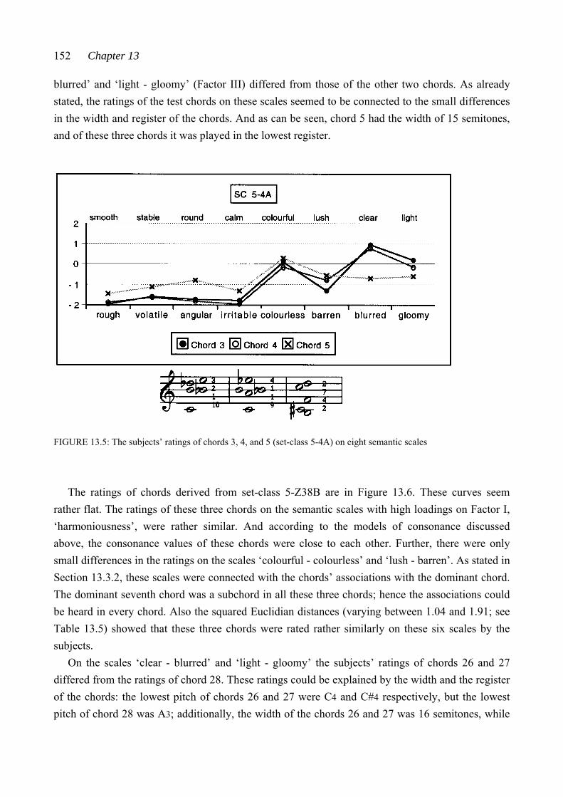
152 Chapter 13
blurred’ and ‘light - gloomy’ (Factor III) differed from those of the other two chords. As already stated, the ratings of the test chords on these scales seemed to be connected to the small differences in the width and register of the chords. And as can be seen, chord 5 had the width of 15 semitones, and of these three chords it was played in the lowest register.
FIGURE 13.5: The subjects’ ratings of chords 3, 4, and 5 (set-class 5-4A) on eight semantic scales
The ratings of chords derived from set-class 5-Z38B are in Figure 13.6. These curves seem
rather flat. The ratings of these three chords on the semantic scales with high loadings on Factor I, ‘harmoniousness’, were rather similar. And according to the models of consonance discussed above, the consonance values of these chords were close to each other. Further, there were only small differences in the ratings on the scales ‘colourful - colourless’ and ‘lush - barren’. As stated in Section 13.3.2, these scales were connected with the chords’ associations with the dominant chord. The dominant seventh chord was a subchord in all these three chords; hence the associations could be heard in every chord. Also the squared Euclidian distances (varying between 1.04 and 1.91; see Table 13.5) showed that these three chords were rated rather similarly on these six scales by the subjects.
On the scales ‘clear - blurred’ and ‘light - gloomy’ the subjects’ ratings of chords 26 and 27 differed from the ratings of chord 28. These ratings could be explained by the width and the register of the chords: the lowest pitch of chords 26 and 27 were C4 and C#4 respectively, but the lowest pitch of chord 28 was A3; additionally, the width of the chords 26 and 27 was 16 semitones, while
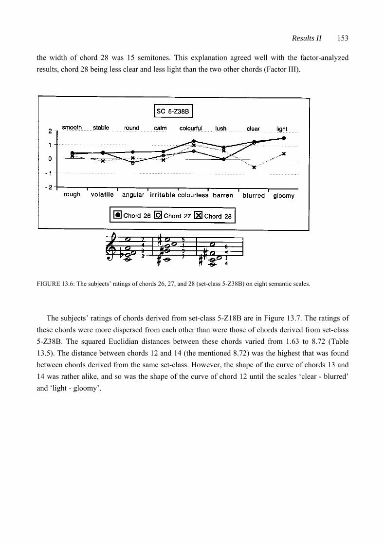
Results II 153
the width of chord 28 was 15 semitones. This explanation agreed well with the factor-analyzed results, chord 28 being less clear and less light than the two other chords (Factor III).
FIGURE 13.6: The subjects’ ratings of chords 26, 27, and 28 (set-class 5-Z38B) on eight semantic scales.
The subjects’ ratings of chords derived from set-class 5-Z18B are in Figure 13.7. The ratings of
these chords were more dispersed from each other than were those of chords derived from set-class 5-Z38B. The squared Euclidian distances between these chords varied from 1.63 to 8.72 (Table 13.5). The distance between chords 12 and 14 (the mentioned 8.72) was the highest that was found between chords derived from the same set-class. However, the shape of the curve of chords 13 and 14 was rather alike, and so was the shape of the curve of chord 12 until the scales ‘clear - blurred’ and ‘light - gloomy’.
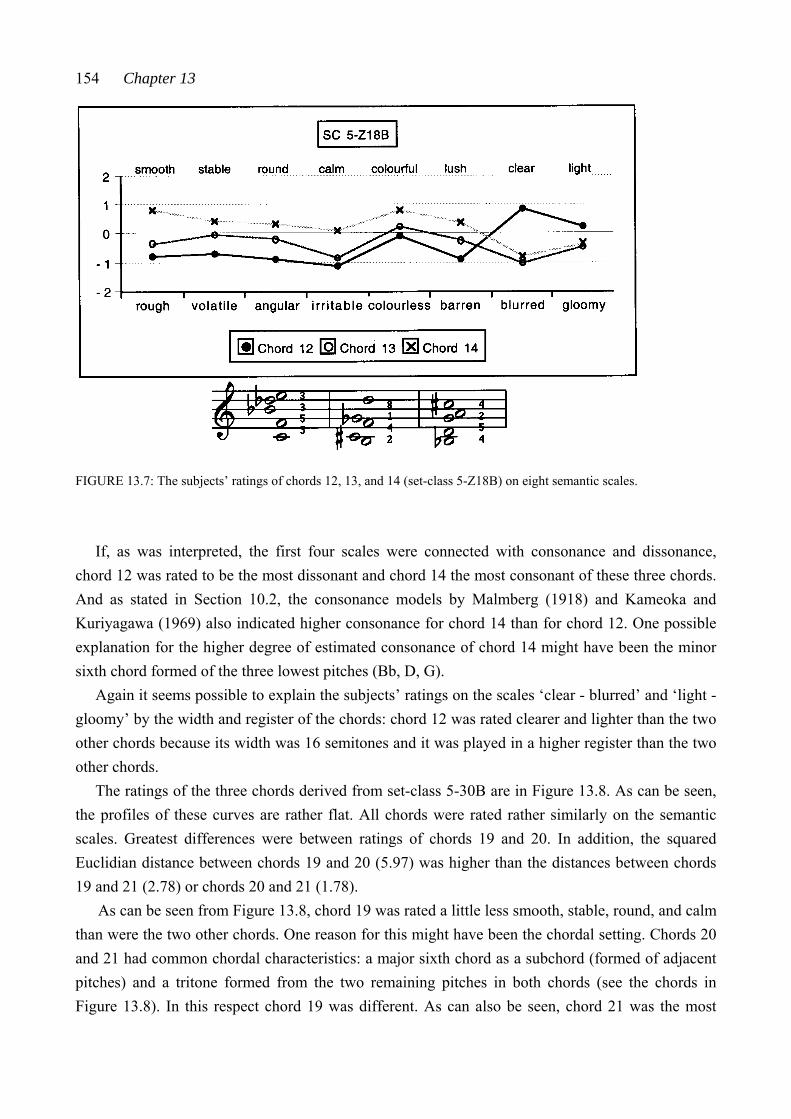
154 Chapter 13
FIGURE 13.7: The subjects’ ratings of chords 12, 13, and 14 (set-class 5-Z18B) on eight semantic scales.
If, as was interpreted, the first four scales were connected with consonance and dissonance,
chord 12 was rated to be the most dissonant and chord 14 the most consonant of these three chords. And as stated in Section 10.2, the consonance models by Malmberg (1918) and Kameoka and Kuriyagawa (1969) also indicated higher consonance for chord 14 than for chord 12. One possible explanation for the higher degree of estimated consonance of chord 14 might have been the minor sixth chord formed of the three lowest pitches (Bb, D, G).
Again it seems possible to explain the subjects’ ratings on the scales ‘clear - blurred’ and ‘light - gloomy’ by the width and register of the chords: chord 12 was rated clearer and lighter than the two other chords because its width was 16 semitones and it was played in a higher register than the two other chords.
The ratings of the three chords derived from set-class 5-30B are in Figure 13.8. As can be seen, the profiles of these curves are rather flat. All chords were rated rather similarly on the semantic scales. Greatest differences were between ratings of chords 19 and 20. In addition, the squared Euclidian distance between chords 19 and 20 (5.97) was higher than the distances between chords 19 and 21 (2.78) or chords 20 and 21 (1.78).
As can be seen from Figure 13.8, chord 19 was rated a little less smooth, stable, round, and calm than were the two other chords. One reason for this might have been the chordal setting. Chords 20 and 21 had common chordal characteristics: a major sixth chord as a subchord (formed of adjacent pitches) and a tritone formed from the two remaining pitches in both chords (see the chords in Figure 13.8). In this respect chord 19 was different. As can also be seen, chord 21 was the most
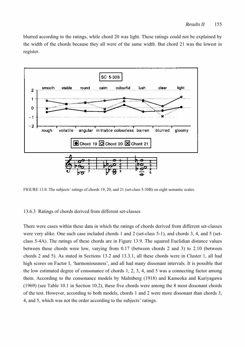
Results II 155
blurred according to the ratings, while chord 20 was light. These ratings could not be explained by the width of the chords because they all were of the same width. But chord 21 was the lowest in register.
FIGURE 13.8: The subjects’ ratings of chords 19, 20, and 21 (set-class 5-30B) on eight semantic scales.
13.6.3 Ratings of chords derived from different set-classes
There were cases within these data in which the ratings of chords derived from different set-classes were very alike. One such case included chords 1 and 2 (set-class 5-1), and chords 3, 4, and 5 (set-class 5-4A). The ratings of these chords are in Figure 13.9. The squared Euclidian distance values between these chords were low, varying from 0.17 (between chords 2 and 3) to 2.10 (between chords 2 and 5). As stated in Sections 13.2 and 13.3.1, all these chords were in Cluster 1, all had high scores on Factor I, ‘harmoniousness’, and all had many dissonant intervals. It is possible that the low estimated degree of consonance of chords 1, 2, 3, 4, and 5 was a connecting factor among them. According to the consonance models by Malmberg (1918) and Kameoka and Kuriyagawa (1969) (see Table 10.1 in Section 10.2), these five chords were among the 8 most dissonant chords of the test. However, according to both models, chords 1 and 2 were more dissonant than chords 3, 4, and 5, which was not the order according to the subjects’ ratings.
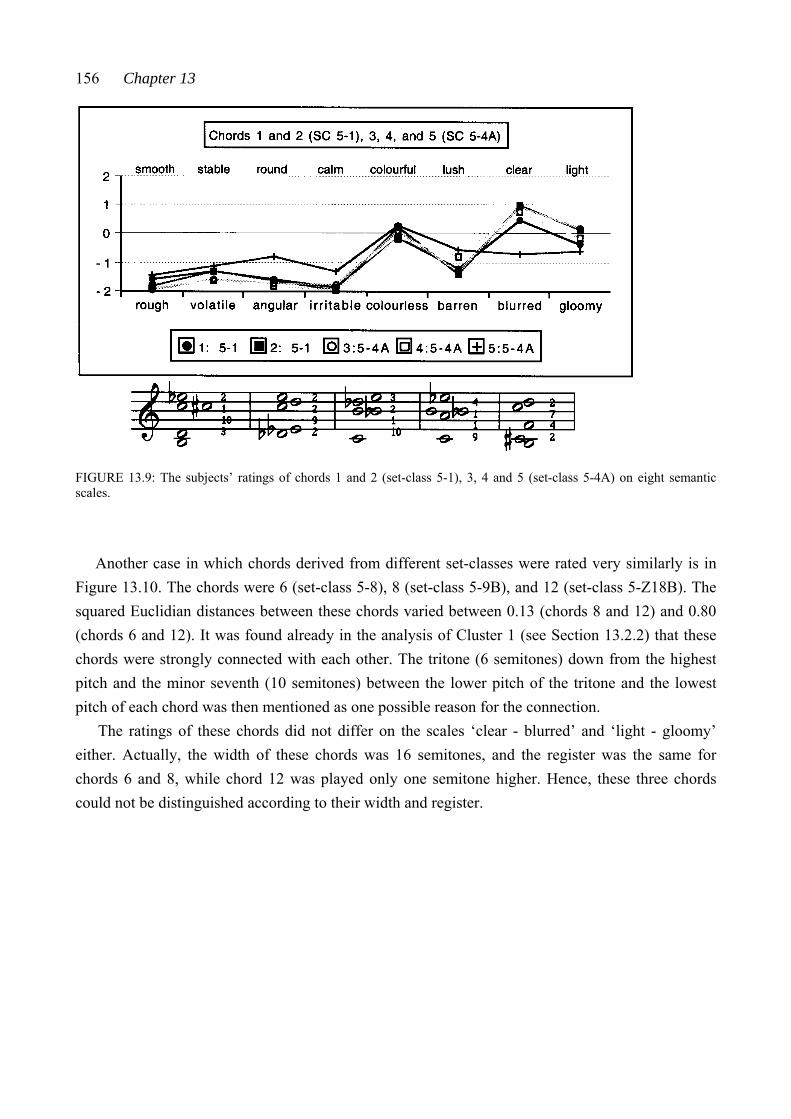
156 Chapter 13
FIGURE 13.9: The subjects’ ratings of chords 1 and 2 (set-class 5-1), 3, 4 and 5 (set-class 5-4A) on eight semantic scales.
Another case in which chords derived from different set-classes were rated very similarly is in
Figure 13.10. The chords were 6 (set-class 5-8), 8 (set-class 5-9B), and 12 (set-class 5-Z18B). The squared Euclidian distances between these chords varied between 0.13 (chords 8 and 12) and 0.80 (chords 6 and 12). It was found already in the analysis of Cluster 1 (see Section 13.2.2) that these chords were strongly connected with each other. The tritone (6 semitones) down from the highest pitch and the minor seventh (10 semitones) between the lower pitch of the tritone and the lowest pitch of each chord was then mentioned as one possible reason for the connection.
The ratings of these chords did not differ on the scales ‘clear - blurred’ and ‘light - gloomy’ either. Actually, the width of these chords was 16 semitones, and the register was the same for chords 6 and 8, while chord 12 was played only one semitone higher. Hence, these three chords could not be distinguished according to their width and register.
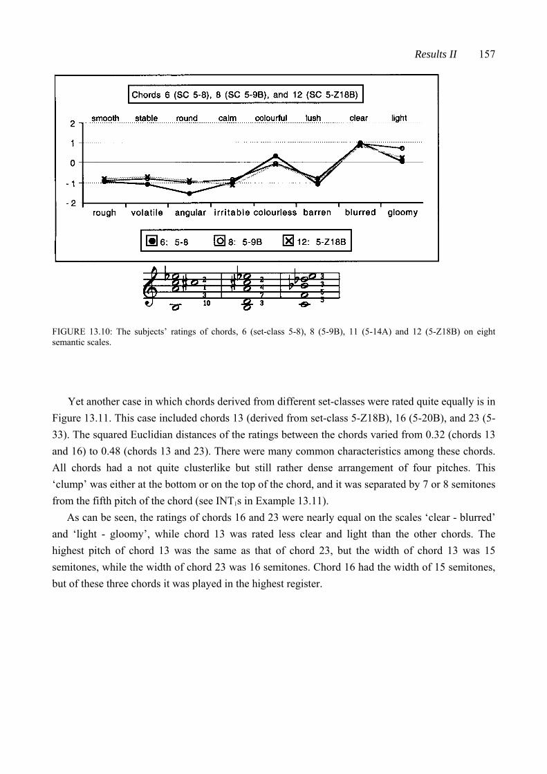
Results II 157
FIGURE 13.10: The subjects’ ratings of chords, 6 (set-class 5-8), 8 (5-9B), 11 (5-14A) and 12 (5-Z18B) on eight semantic scales.
Yet another case in which chords derived from different set-classes were rated quite equally is in
Figure 13.11. This case included chords 13 (derived from set-class 5-Z18B), 16 (5-20B), and 23 (5-33). The squared Euclidian distances of the ratings between the chords varied from 0.32 (chords 13 and 16) to 0.48 (chords 13 and 23). There were many common characteristics among these chords. All chords had a not quite clusterlike but still rather dense arrangement of four pitches. This ‘clump’ was either at the bottom or on the top of the chord, and it was separated by 7 or 8 semitones from the fifth pitch of the chord (see INT1s in Example 13.11).
As can be seen, the ratings of chords 16 and 23 were nearly equal on the scales ‘clear - blurred’ and ‘light - gloomy’, while chord 13 was rated less clear and light than the other chords. The highest pitch of chord 13 was the same as that of chord 23, but the width of chord 13 was 15 semitones, while the width of chord 23 was 16 semitones. Chord 16 had the width of 15 semitones, but of these three chords it was played in the highest register.
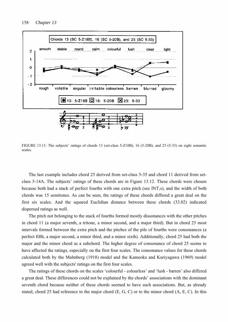
158 Chapter 13
FIGURE 13.11: The subjects’ ratings of chords 13 (set-class 5-Z18B), 16 (5-20B), and 23 (5-33) on eight semantic scales.
The last example includes chord 25 derived from set-class 5-35 and chord 11 derived from set-
class 5-14A. The subjects’ ratings of these chords are in Figure 13.12. These chords were chosen because both had a stack of perfect fourths with one extra pitch (see INT1s), and the width of both chords was 15 semitones. As can be seen, the ratings of these chords differed a great deal on the first six scales. And the squared Euclidian distance between these chords (33.02) indicated dispersed ratings as well.
The pitch not belonging to the stack of fourths formed mostly dissonances with the other pitches in chord 11 (a major seventh, a tritone, a minor second, and a major third). But in chord 25 most intervals formed between the extra pitch and the pitches of the pile of fourths were consonances (a perfect fifth, a major second, a minor third, and a minor sixth). Additionally, chord 25 had both the major and the minor chord as a subchord. The higher degree of consonance of chord 25 seems to have affected the ratings, especially on the first four scales. The consonance values for these chords calculated both by the Malmberg (1918) model and the Kameoka and Kuriyagawa (1969) model agreed well with the subjects' ratings on the first four scales.
The ratings of these chords on the scales ‘colourful - colourless’ and ‘lush - barren’ also differed a great deal. These differences could not be explained by the chords’ associations with the dominant seventh chord because neither of these chords seemed to have such associations. But, as already stated, chord 25 had reference to the major chord (E, G, C) or to the minor chord (A, E, C). In this
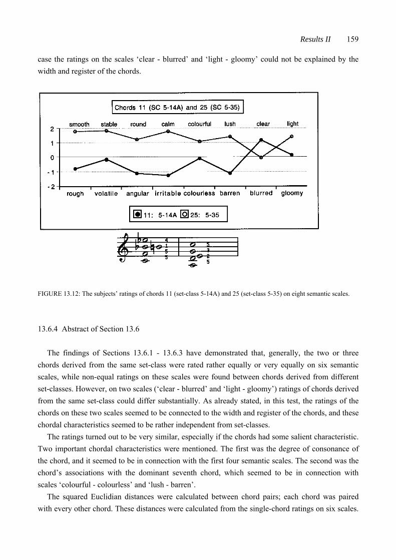
Results II 159
case the ratings on the scales ‘clear - blurred’ and ‘light - gloomy’ could not be explained by the width and register of the chords.
FIGURE 13.12: The subjects’ ratings of chords 11 (set-class 5-14A) and 25 (set-class 5-35) on eight semantic scales.
13.6.4 Abstract of Section 13.6 The findings of Sections 13.6.1 - 13.6.3 have demonstrated that, generally, the two or three
chords derived from the same set-class were rated rather equally or very equally on six semantic scales, while non-equal ratings on these scales were found between chords derived from different set-classes. However, on two scales (‘clear - blurred’ and ‘light - gloomy’) ratings of chords derived from the same set-class could differ substantially. As already stated, in this test, the ratings of the chords on these two scales seemed to be connected to the width and register of the chords, and these chordal characteristics seemed to be rather independent from set-classes.
The ratings turned out to be very similar, especially if the chords had some salient characteristic. Two important chordal characteristics were mentioned. The first was the degree of consonance of the chord, and it seemed to be in connection with the first four semantic scales. The second was the chord’s associations with the dominant seventh chord, which seemed to be in connection with scales ‘colourful - colourless’ and ‘lush - barren’.
The squared Euclidian distances were calculated between chord pairs; each chord was paired with every other chord. These distances were calculated from the single-chord ratings on six scales.
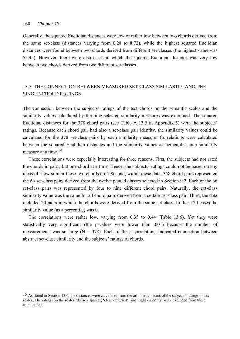
160 Chapter 13
Generally, the squared Euclidian distances were low or rather low between two chords derived from the same set-class (distances varying from 0.28 to 8.72), while the highest squared Euclidian distances were found between two chords derived from different set-classes (the highest value was 55.45). However, there were also cases in which the squared Euclidian distance was very low between two chords derived from two different set-classes.
13.7 THE CONNECTION BETWEEN MEASURED SET-CLASS SIMILARITY AND THE SINGLE-CHORD RATINGS
The connection between the subjects’ ratings of the test chords on the semantic scales and the similarity values calculated by the nine selected similarity measures was examined. The squared Euclidian distances for the 378 chord pairs (see Table A 13.5 in Appendix 5) were the subjects’ ratings. Because each chord pair had also a set-class pair identity, the similarity values could be calculated for the 378 set-class pairs by each similarity measure. Correlations were calculated between the squared Euclidian distances and the similarity values as percentiles, one similarity measure at a time.15
These correlations were especially interesting for three reasons. First, the subjects had not rated the chords in pairs, but one chord at a time. Hence, the subjects’ ratings could not be based on any ideas of ‘how similar these two chords are’. Second, within these data, 358 chord pairs represented the 66 set-class pairs derived from the twelve pentad classes selected in Section 9.2. Each of the 66 set-class pairs was represented by four to nine different chord pairs. Naturally, the set-class similarity value was the same for all chord pairs derived from a certain set-class pair. Third, the data included 20 pairs in which the chords were derived from the same set-class. In these 20 cases the similarity value (as a percentile) was 0.
The correlations were rather low, varying from 0.35 to 0.44 (Table 13.6). Yet they were statistically very significant (the p-values were lower than .001) because the number of measurements was so large (N = 378). Each of these correlations indicated connection between abstract set-class similarity and the subjects’ ratings of chords.
15 As stated in Section 13.6, the distances were calculated from the arithmetic means of the subjects’ ratings on six scales. The ratings on the scales ‘dense - sparse’, ‘clear - blurred’, and ‘light - gloomy’ were excluded from these calculations.
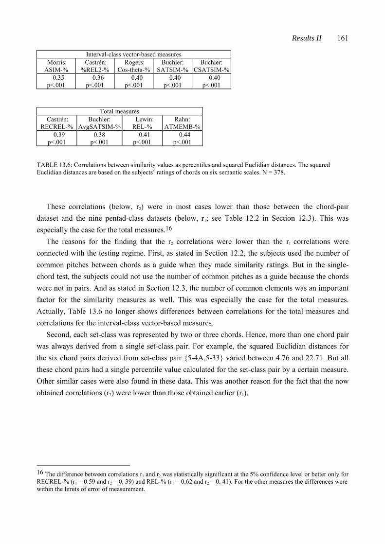
Results II 161
Interval-class vector-based measures Morris: ASIM-%
Castrén: %REL2-%
Rogers: Cos-theta-%
Buchler: SATSIM-%
Buchler: CSATSIM-%
0.35 p<.001
0.36 p<.001
0.40 p<.001
0.40 p<.001
0.40 p<.001
Total measures Castrén:
RECREL-% Buchler:
AvgSATSIM-% Lewin: REL-%
Rahn: ATMEMB-%
0.39 p<.001
0.38 p<.001
0.41 p<.001
0.44 p<.001
TABLE 13.6: Correlations between similarity values as percentiles and squared Euclidian distances. The squared Euclidian distances are based on the subjects’ ratings of chords on six semantic scales. N = 378.
These correlations (below, r2) were in most cases lower than those between the chord-pair dataset and the nine pentad-class datasets (below, r1; see Table 12.2 in Section 12.3). This was especially the case for the total measures.16
The reasons for the finding that the r2 correlations were lower than the r1 correlations were connected with the testing regime. First, as stated in Section 12.2, the subjects used the number of common pitches between chords as a guide when they made similarity ratings. But in the single-chord test, the subjects could not use the number of common pitches as a guide because the chords were not in pairs. And as stated in Section 12.3, the number of common elements was an important factor for the similarity measures as well. This was especially the case for the total measures. Actually, Table 13.6 no longer shows differences between correlations for the total measures and correlations for the interval-class vector-based measures.
Second, each set-class was represented by two or three chords. Hence, more than one chord pair was always derived from a single set-class pair. For example, the squared Euclidian distances for the six chord pairs derived from set-class pair {5-4A,5-33} varied between 4.76 and 22.71. But all these chord pairs had a single percentile value calculated for the set-class pair by a certain measure. Other similar cases were also found in these data. This was another reason for the fact that the now obtained correlations (r2) were lower than those obtained earlier (r1).
16 The difference between correlations r1 and r2 was statistically significant at the 5% confidence level or better only for RECREL-% (r1 = 0.59 and r2 = 0. 39) and REL-% (r1 = 0.62 and r2 = 0. 41). For the other measures the differences were within the limits of error of measurement.
162 Chapter 13
13.8 SUMMARY OF CHAPTER 13
This chapter examined the single-chord dataset by many analyses. The results of these analyses were compared with each other and with results derived from the multidimensional scaling analysis of the chord-pair dataset. Additionally, the subjects’ single-chord ratings were explained by chordal characteristics and these characteristics were compared with properties of the set-classes from which the chords were derived.
Three chordal characteristics were found to guide the subjects’ ratings of single chords in this study. These characteristics were found in both the hierarchical clustering analysis and the factor analysis of the dataset. The first and the most important one was the degree of estimated consonance of the chords. The second characteristic was interpreted as the perceived associations with the dominant seventh chord or with the major chord. The third one was the width and register of the chords. The first two characteristics were also found when the chord-pair dataset was analyzed in Chapter 12.
The degree of estimated consonance of the chords seemed to be in connection with the subjects’ ratings on four semantic scales (‘smooth - rough’, ‘stable - volatile’, ‘round - angular’, and ‘calm - irritable’). This characteristic could also be explained by the number of instances of interval-classes 1 and 6 included in the set-classes from which the chords were derived. The chords’ perceived associations with the dominant seventh chord or with the major chord seemed to be in connection with scales ‘colourful - colourless’ and ‘lush - barren’. These associations could be explained by the total number of instances of subset-classes 4-27B and 3-11B included in the set-classes.
The arrangement of the pitches, that is, the chordal setting, also seemed to be important for the subjects’ ratings. The two chordal characteristics mentioned could be explained by the set-class properties only to some extent. Additionally, the third characteristic, namely, the width and register of the chords, seemed to be bound to chordal setting, not to set-class properties. Hence, it seemed that the subjects’ single-chord ratings were based on both abstract set-class properties and chordal setting (as were the subjects’ closeness ratings as well).
The degree of estimated consonance of chords was also compared to theoretical consonance values for chords calculated by two consonance models. The correlation between the factor scores on Factor I (‘harmoniousness’) and the consonance values for chords calculated by the Malmberg (1918) model was high (0.81). The corresponding correlation for the Kameoka and Kuriyagawa (1969) model was lower (0.70). These statistically very significant correlations (p < .001) indicated that the theoretical consonance values fitted well with the factor-analyzed solution of the single-chord dataset. Hence, the consonance models and the analysis validated each other. As stated in Section 5.2, the subjects of the tests of Kameoka and Kuriyagawa were non-musicians, while the subjects of the tests of Malmberg were musically experienced. Also in the present study, musically

Results II 163
trained subjects rated the chords. This might have been one reason for the fact that there was a higher correlation for the Malmberg model than for the Kameoka and Kuriyagawa model.
CHAPTER FOURTEEN RESULTS III: THE PENTAD-CLASS DATASETS
This chapter deals with results analyzed from the nine pentad-class datasets. Each dataset consisted of similarity values as percentiles for 66 set-class pairs formed of twelve pentad classes.1 In each dataset these percentiles were calculated by one of the nine similarity measures selected in Chapter 7.2
Section 14.1 discusses the multidimensional scaling analysis made of the datasets and the number of dimensions appropriate for the solutions. Section 14.2 examines the solutions derived from the five interval-class vector-based measures. Section 14.3 examines the solutions derived from the four total measures. The connection between the dimensions analyzed from the chord-pair dataset and the dimensions analyzed from the nine pentad-class datasets is discussed in Section 14.4. The most important results of Chapter 14 are summarised in Section 14.5.
14.1 MULTIDIMENSIONAL SCALING ANALYSIS APPLIED TO THE NINE PENTAD-CLASS DATASETS
The nine pentad-class datasets were analyzed by multidimensional scaling, one dataset at a time.3 In these analyses, the objects were the twelve pentad classes. The similarity values as percentiles were considered to be distances between set-classes. All these distances were on the same measurement scale, i.e., the input of each analysis was matrix conditional.
When the SPSS 8.0 multidimensional scaling algorithm (Alscal) was applied to these datasets, each dataset was forced to fit into three dimensions. The goodness-of-fit measures in most cases 1 As stated in Section 8.2, the percentiles are from 0 to 100, with 0 indicating maximum similarity (the shortest distance between set-classes). When the similarity values are given as percentiles, the symbol -% is added to the name of the measure, for example, ASIM-%. 2 As stated in Section 9.4, Cosθ-% represents both Cosθ-% and IcVD2-%. 3 For multidimensional scaling, see Definitions III.
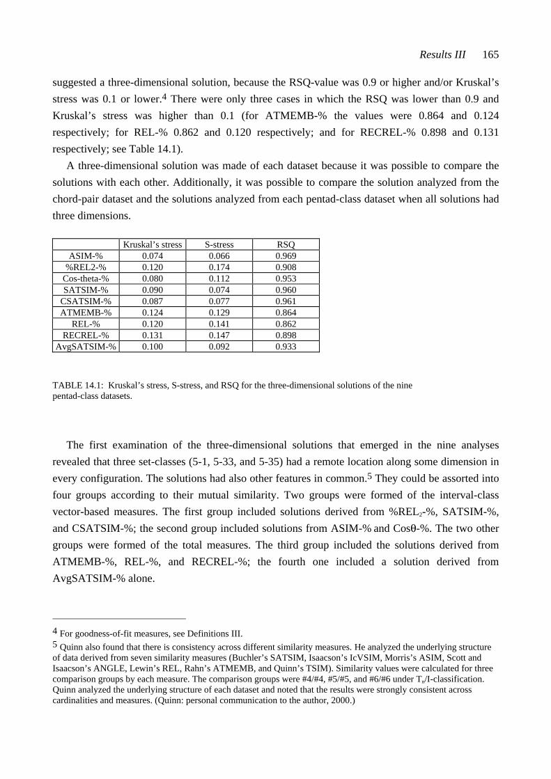
Results III 165
suggested a three-dimensional solution, because the RSQ-value was 0.9 or higher and/or Kruskal’s stress was 0.1 or lower.4 There were only three cases in which the RSQ was lower than 0.9 and Kruskal’s stress was higher than 0.1 (for ATMEMB-% the values were 0.864 and 0.124 respectively; for REL-% 0.862 and 0.120 respectively; and for RECREL-% 0.898 and 0.131 respectively; see Table 14.1).
A three-dimensional solution was made of each dataset because it was possible to compare the solutions with each other. Additionally, it was possible to compare the solution analyzed from the chord-pair dataset and the solutions analyzed from each pentad-class dataset when all solutions had three dimensions.
Kruskal’s stress S-stress RSQ ASIM-% 0.074 0.066 0.969
%REL2-% 0.120 0.174 0.908 Cos-theta-% 0.080 0.112 0.953 SATSIM-% 0.090 0.074 0.960
CSATSIM-% 0.087 0.077 0.961 ATMEMB-% 0.124 0.129 0.864
REL-% 0.120 0.141 0.862 RECREL-% 0.131 0.147 0.898
AvgSATSIM-% 0.100 0.092 0.933
TABLE 14.1: Kruskal’s stress, S-stress, and RSQ for the three-dimensional solutions of the nine pentad-class datasets.
The first examination of the three-dimensional solutions that emerged in the nine analyses
revealed that three set-classes (5-1, 5-33, and 5-35) had a remote location along some dimension in every configuration. The solutions had also other features in common.5 They could be assorted into four groups according to their mutual similarity. Two groups were formed of the interval-class vector-based measures. The first group included solutions derived from %REL2-%, SATSIM-%, and CSATSIM-%; the second group included solutions from ASIM-% and Cosθ-%. The two other groups were formed of the total measures. The third group included the solutions derived from ATMEMB-%, REL-%, and RECREL-%; the fourth one included a solution derived from AvgSATSIM-% alone.
4 For goodness-of-fit measures, see Definitions III. 5 Quinn also found that there is consistency across different similarity measures. He analyzed the underlying structure of data derived from seven similarity measures (Buchler’s SATSIM, Isaacson’s IcVSIM, Morris’s ASIM, Scott and Isaacson’s ANGLE, Lewin’s REL, Rahn’s ATMEMB, and Quinn’s TSIM). Similarity values were calculated for three comparison groups by each measure. The comparison groups were #4/#4, #5/#5, and #6/#6 under Tn/I-classification. Quinn analyzed the underlying structure of each dataset and noted that the results were strongly consistent across cardinalities and measures. (Quinn: personal communication to the author, 2000.)
166 Chapter 14
14.2 THE THREE-DIMENSIONAL SOLUTIONS ANALYZED FROM DATASETS DERIVED FROM THE INTERVAL-CLASS VECTOR-BASED MEASURES
The next three sections examine the three-dimensional solutions derived from the selected interval-class vector-based measures. The properties of the interval-class vectors will be used to interpret the solutions. The interval-class vectors of the three set-classes with remote locations along some dimension (set-classes 5-1, 5-33, and 5-35) will be analyzed first (Section 14.2.1). This is done because it seems likely that the properties that are prominent in the interval-class vectors of these set-classes would best guide the interpretation of the dimensions. The three-dimensional solutions derived from the interval-class vector-based measures will be discussed in Sections 14.2.2 (%REL2-%, SATSIM-%, and CSATSIM-%), and 14.2.3 (ASIM-% and Cosθ-%).
14.2.1 The interval-class contents of set-classes 5-1, 5-33, and 5-35
Set-class 5-1 is a 5-pc chromatic class, and set-class 5-33 is the 5-pc whole-tone class. Set-class 5-35 is the pentatonic class, containing no instances of interval-class 1 or 6. It is also known as the (five-element) cycle-of-fifths class. The interval-class vectors of these set-classes are in Example 14.1. As can be seen, these vectors have both peaks and zero components. Additionally, all vectors have at least one maximum component.6 It seems that all interval-class vector-based measures reacted to the uneven distribution of the interval-class instances (the ‘peakedness’ of the vectors) as well as to the maximum components and zero components, despite the different aspects on which these measures were based and despite the differences in the calculation processes.
ICV(5-1) = [4 3 2 1 0 0]
ICV(5-33) = [0 4 0 4 0 2]
ICV(5-35) = [0 3 2 1 4 0]
EXAMPLE 14.1: The interval-class vectors of set-classes 5-1, 5-33 and 5-35. In the vectors the maximum components are in bold print.
The maximum component in the interval-class vector of set-class 5-1 is in index 1 (interval-class
1), and the peaks are in indexes 1 and 2. Below, the total number of interval-class 1 and 2 instances will be called the ‘ic 1 and 2 content’. The high ic 1 and 2 content is typical to set-class 5-1, since 6 The terms ‘peak’, ‘maximum component’, and ‘zero component’ were defined in Section 9.1.
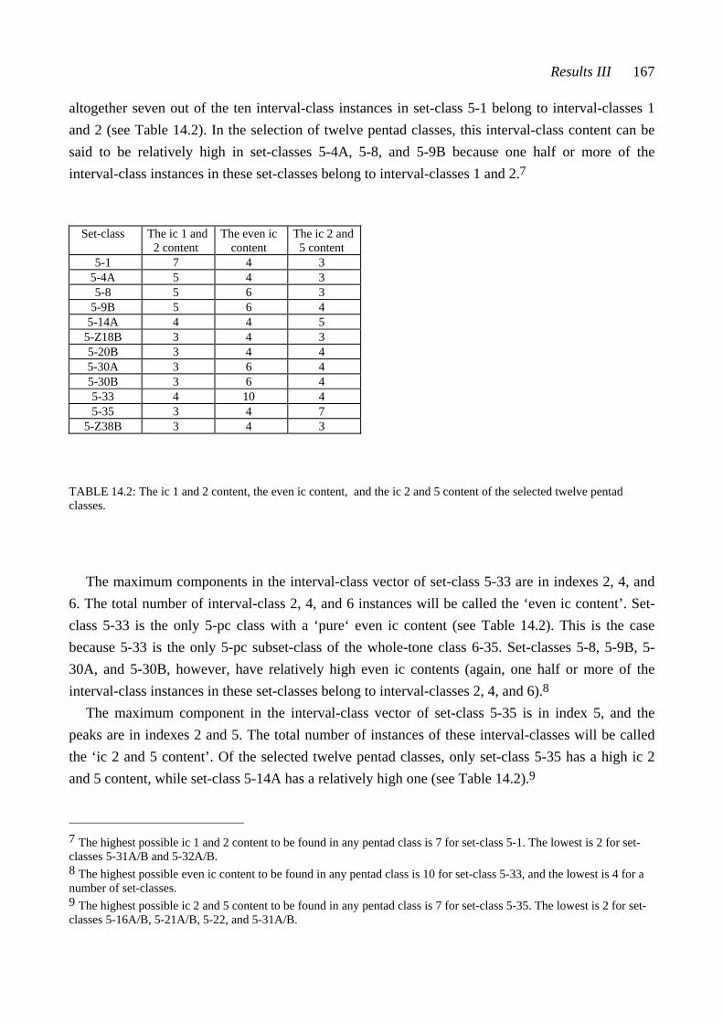
Results III 167
altogether seven out of the ten interval-class instances in set-class 5-1 belong to interval-classes 1 and 2 (see Table 14.2). In the selection of twelve pentad classes, this interval-class content can be said to be relatively high in set-classes 5-4A, 5-8, and 5-9B because one half or more of the interval-class instances in these set-classes belong to interval-classes 1 and 2.7
Set-class The ic 1 and 2 content
The even ic content
The ic 2 and 5 content
5-1 7 4 3 5-4A 5 4 3 5-8 5 6 3
5-9B 5 6 4 5-14A 4 4 5
5-Z18B 3 4 3 5-20B 3 4 4 5-30A 3 6 4 5-30B 3 6 4 5-33 4 10 4 5-35 3 4 7
5-Z38B 3 4 3 TABLE 14.2: The ic 1 and 2 content, the even ic content, and the ic 2 and 5 content of the selected twelve pentad classes.
The maximum components in the interval-class vector of set-class 5-33 are in indexes 2, 4, and
6. The total number of interval-class 2, 4, and 6 instances will be called the ‘even ic content’. Set-class 5-33 is the only 5-pc class with a ‘pure‘ even ic content (see Table 14.2). This is the case because 5-33 is the only 5-pc subset-class of the whole-tone class 6-35. Set-classes 5-8, 5-9B, 5-30A, and 5-30B, however, have relatively high even ic contents (again, one half or more of the interval-class instances in these set-classes belong to interval-classes 2, 4, and 6).8
The maximum component in the interval-class vector of set-class 5-35 is in index 5, and the peaks are in indexes 2 and 5. The total number of instances of these interval-classes will be called the ‘ic 2 and 5 content’. Of the selected twelve pentad classes, only set-class 5-35 has a high ic 2 and 5 content, while set-class 5-14A has a relatively high one (see Table 14.2).9
7 The highest possible ic 1 and 2 content to be found in any pentad class is 7 for set-class 5-1. The lowest is 2 for set-classes 5-31A/B and 5-32A/B. 8 The highest possible even ic content to be found in any pentad class is 10 for set-class 5-33, and the lowest is 4 for a number of set-classes. 9 The highest possible ic 2 and 5 content to be found in any pentad class is 7 for set-class 5-35. The lowest is 2 for set-classes 5-16A/B, 5-21A/B, 5-22, and 5-31A/B.
168 Chapter 14
These three interval-class content categories will be used to guide the interpretation of the solutions analyzed from the nine pentad-class datasets.10 As the interval-class contents are quantities, it will be possible to calculate correlations between them and the locations of set-classes in each dimension (the locations are defined by the set-class coordinates). The correlations will be calculated to confirm the interpretations of the dimensions.
14.2.2 The three-dimensional solutions derived from %REL2-%, SATSIM-%, and CSATSIM-%
The three-dimensional solutions derived from %REL2-%, SATSIM-%, and CSATSIM-% were very closely related. Correlations were calculated between solutions derived from these three measures. When this was done, the locations of the set-classes along the three dimensions of one measure were compared with the locations of the set-classes along the three dimensions of another measure. Each of the twelve set-classes had coordinates in each dimension; hence, the number of measurements was 3*12 = 36. The correlations were r = 0.99 between SATSIM-% and CSATSIM-%, r = 0.97 between %REL2-% and CSATSIM-%, and r = 0.98 between %REL2-% and SATSIM-%. These very high correlations indicated that the set-classes had nearly equal locations along the three dimensions of each measure.
The solution of each measure was rotated to make the dimensions easier to interpret. Dimensions 1 and 2 of %REL2-% were rotated approximately 30 degrees clockwise, and dimensions 1 and 2 of SATSIM-% and CSATSIM-% were rotated approximately 25 degrees clockwise. The configurations (the pictures of the three-dimensional solutions) derived from SATSIM-%, CSATSIM-%, and %REL2-% after rotation are in Figure 14.1. In this figure, only the set-classes with the most remote locations along each dimension are shown. All set-class coordinates along the three dimensions are in Table A 14.1 in Appendix 5.
The set-class with the most remote location at the positive end of dimension 1 (after rotation) was 5-1. The next two, with much lower coordinates, were set-classes 5-4A and 5-8 (owing to lack of space, only set-class 5-4A is shown in Figure 14.1). At the negative end of dimension 1, the set-classes with the most remote locations were 5-30A and 5-30B (with the same coordinates), and the next was set-class 5-20B. The set-classes at the positive end had higher ic 1 and 2 contents than the set-classes at the negative end. This interpretation was tested by calculating correlations between
10 When Quinn analyzed the datasets he had selected, seven explanatory factors were usually found. These factors were: A: ‘high content of interval-class 1’ (‘chromatic’); B: ‘high content of interval-class 2, with fairly even distribution of other interval-classes’; C: ‘high content of interval-class 5’ (‘circle-of-fifths’); D: ‘high content of interval-class 1 and interval-class 6, with low interval-class 4 content’; E: ‘high content of interval-class 4, but low interval-class 2 and interval-class 6 content’; F: ‘high content of all even interval-classes’ (‘whole-tone’); G: ‘high content of interval-class 3 and interval-class 6’ (Quinn: personal communication to the author, 2000)
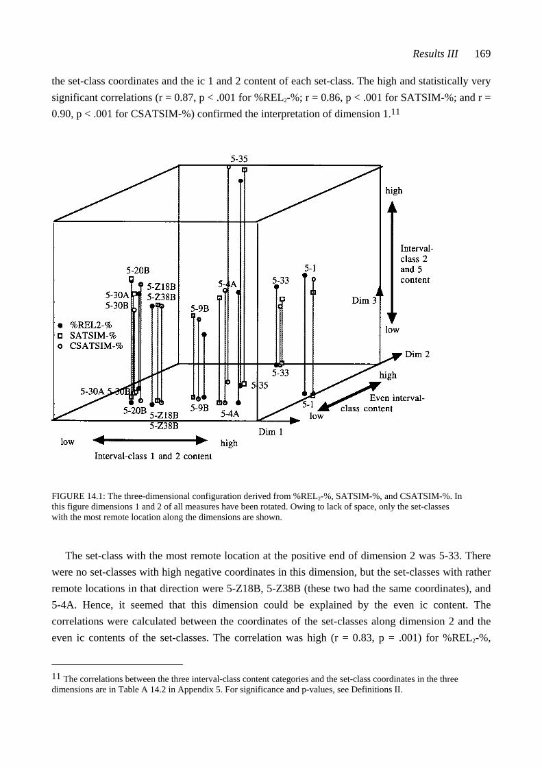
Results III 169
the set-class coordinates and the ic 1 and 2 content of each set-class. The high and statistically very significant correlations (r = 0.87, p < .001 for %REL2-%; r = 0.86, p < .001 for SATSIM-%; and r = 0.90, p < .001 for CSATSIM-%) confirmed the interpretation of dimension 1.11
FIGURE 14.1: The three-dimensional configuration derived from %REL2-%, SATSIM-%, and CSATSIM-%. In this figure dimensions 1 and 2 of all measures have been rotated. Owing to lack of space, only the set-classes with the most remote location along the dimensions are shown.
The set-class with the most remote location at the positive end of dimension 2 was 5-33. There were no set-classes with high negative coordinates in this dimension, but the set-classes with rather remote locations in that direction were 5-Z18B, 5-Z38B (these two had the same coordinates), and 5-4A. Hence, it seemed that this dimension could be explained by the even ic content. The correlations were calculated between the coordinates of the set-classes along dimension 2 and the even ic contents of the set-classes. The correlation was high (r = 0.83, p = .001) for %REL2-%,
11 The correlations between the three interval-class content categories and the set-class coordinates in the three dimensions are in Table A 14.2 in Appendix 5. For significance and p-values, see Definitions II.
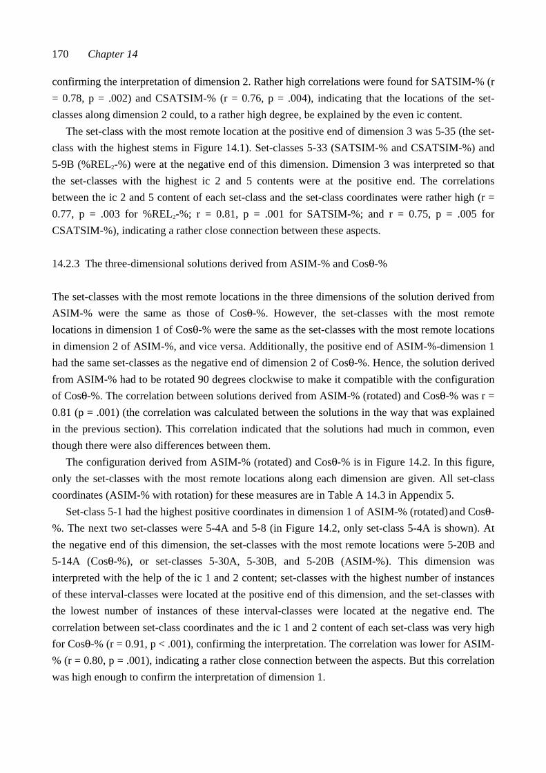
170 Chapter 14
confirming the interpretation of dimension 2. Rather high correlations were found for SATSIM-% (r = 0.78, p = .002) and CSATSIM-% (r = 0.76, p = .004), indicating that the locations of the set-classes along dimension 2 could, to a rather high degree, be explained by the even ic content.
The set-class with the most remote location at the positive end of dimension 3 was 5-35 (the set-class with the highest stems in Figure 14.1). Set-classes 5-33 (SATSIM-% and CSATSIM-%) and 5-9B (%REL2-%) were at the negative end of this dimension. Dimension 3 was interpreted so that the set-classes with the highest ic 2 and 5 contents were at the positive end. The correlations between the ic 2 and 5 content of each set-class and the set-class coordinates were rather high (r = 0.77, p = .003 for %REL2-%; r = 0.81, p = .001 for SATSIM-%; and r = 0.75, p = .005 for CSATSIM-%), indicating a rather close connection between these aspects.
14.2.3 The three-dimensional solutions derived from ASIM-% and Cosθ-%
The set-classes with the most remote locations in the three dimensions of the solution derived from ASIM-% were the same as those of Cosθ-%. However, the set-classes with the most remote locations in dimension 1 of Cosθ-% were the same as the set-classes with the most remote locations in dimension 2 of ASIM-%, and vice versa. Additionally, the positive end of ASIM-%-dimension 1 had the same set-classes as the negative end of dimension 2 of Cosθ-%. Hence, the solution derived from ASIM-% had to be rotated 90 degrees clockwise to make it compatible with the configuration of Cosθ-%. The correlation between solutions derived from ASIM-% (rotated) and Cosθ-% was r = 0.81 (p = .001) (the correlation was calculated between the solutions in the way that was explained in the previous section). This correlation indicated that the solutions had much in common, even though there were also differences between them.
The configuration derived from ASIM-% (rotated) and Cosθ-% is in Figure 14.2. In this figure, only the set-classes with the most remote locations along each dimension are given. All set-class coordinates (ASIM-% with rotation) for these measures are in Table A 14.3 in Appendix 5.
Set-class 5-1 had the highest positive coordinates in dimension 1 of ASIM-% (rotated) and Cosθ-%. The next two set-classes were 5-4A and 5-8 (in Figure 14.2, only set-class 5-4A is shown). At the negative end of this dimension, the set-classes with the most remote locations were 5-20B and 5-14A (Cosθ-%), or set-classes 5-30A, 5-30B, and 5-20B (ASIM-%). This dimension was interpreted with the help of the ic 1 and 2 content; set-classes with the highest number of instances of these interval-classes were located at the positive end of this dimension, and the set-classes with the lowest number of instances of these interval-classes were located at the negative end. The correlation between set-class coordinates and the ic 1 and 2 content of each set-class was very high for Cosθ-% (r = 0.91, p < .001), confirming the interpretation. The correlation was lower for ASIM-% (r = 0.80, p = .001), indicating a rather close connection between the aspects. But this correlation was high enough to confirm the interpretation of dimension 1.
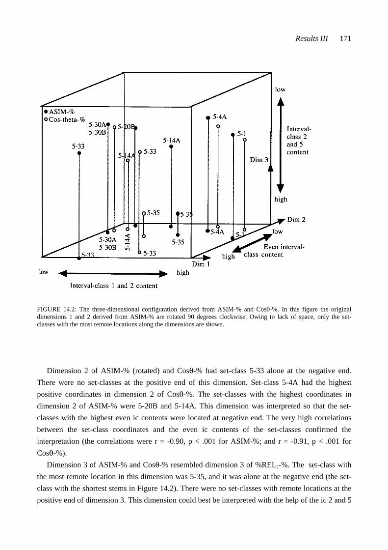
Results III 171
FIGURE 14.2: The three-dimensional configuration derived from ASIM-% and Cosθ-%. In this figure the original dimensions 1 and 2 derived from ASIM-% are rotated 90 degrees clockwise. Owing to lack of space, only the set-classes with the most remote locations along the dimensions are shown.
Dimension 2 of ASIM-% (rotated) and Cosθ-% had set-class 5-33 alone at the negative end.
There were no set-classes at the positive end of this dimension. Set-class 5-4A had the highest positive coordinates in dimension 2 of Cosθ-%. The set-classes with the highest coordinates in dimension 2 of ASIM-% were 5-20B and 5-14A. This dimension was interpreted so that the set-classes with the highest even ic contents were located at negative end. The very high correlations between the set-class coordinates and the even ic contents of the set-classes confirmed the interpretation (the correlations were r = -0.90, p < .001 for ASIM-%; and r = -0.91, p < .001 for Cosθ-%).
Dimension 3 of ASIM-% and Cosθ-% resembled dimension 3 of %REL2-%. The set-class with the most remote location in this dimension was 5-35, and it was alone at the negative end (the set-class with the shortest stems in Figure 14.2). There were no set-classes with remote locations at the positive end of dimension 3. This dimension could best be interpreted with the help of the ic 2 and 5
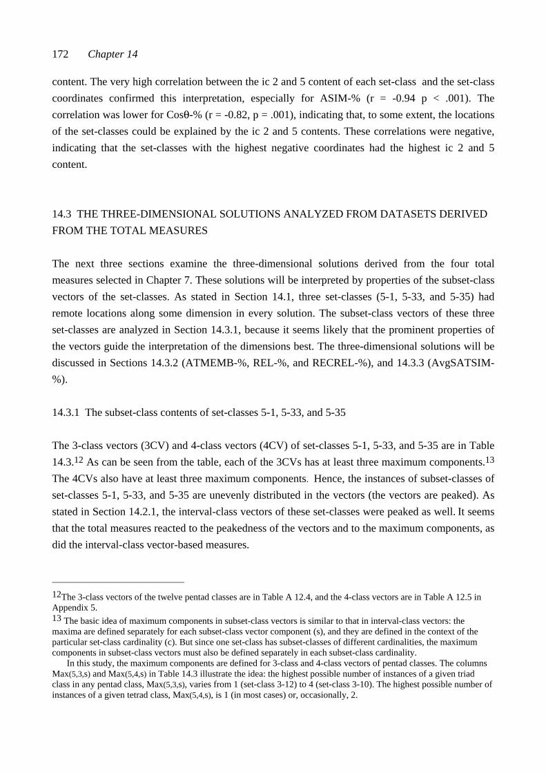
172 Chapter 14
content. The very high correlation between the ic 2 and 5 content of each set-class and the set-class coordinates confirmed this interpretation, especially for ASIM-% (r = -0.94 p < .001). The correlation was lower for Cosθ-% (r = -0.82, p = .001), indicating that, to some extent, the locations of the set-classes could be explained by the ic 2 and 5 contents. These correlations were negative, indicating that the set-classes with the highest negative coordinates had the highest ic 2 and 5 content.
14.3 THE THREE-DIMENSIONAL SOLUTIONS ANALYZED FROM DATASETS DERIVED FROM THE TOTAL MEASURES
The next three sections examine the three-dimensional solutions derived from the four total measures selected in Chapter 7. These solutions will be interpreted by properties of the subset-class vectors of the set-classes. As stated in Section 14.1, three set-classes (5-1, 5-33, and 5-35) had remote locations along some dimension in every solution. The subset-class vectors of these three set-classes are analyzed in Section 14.3.1, because it seems likely that the prominent properties of the vectors guide the interpretation of the dimensions best. The three-dimensional solutions will be discussed in Sections 14.3.2 (ATMEMB-%, REL-%, and RECREL-%), and 14.3.3 (AvgSATSIM-%).
14.3.1 The subset-class contents of set-classes 5-1, 5-33, and 5-35
The 3-class vectors (3CV) and 4-class vectors (4CV) of set-classes 5-1, 5-33, and 5-35 are in Table 14.3.12 As can be seen from the table, each of the 3CVs has at least three maximum components.13 The 4CVs also have at least three maximum components. Hence, the instances of subset-classes of set-classes 5-1, 5-33, and 5-35 are unevenly distributed in the vectors (the vectors are peaked). As stated in Section 14.2.1, the interval-class vectors of these set-classes were peaked as well. It seems that the total measures reacted to the peakedness of the vectors and to the maximum components, as did the interval-class vector-based measures.
12The 3-class vectors of the twelve pentad classes are in Table A 12.4, and the 4-class vectors are in Table A 12.5 in Appendix 5. 13 The basic idea of maximum components in subset-class vectors is similar to that in interval-class vectors: the maxima are defined separately for each subset-class vector component (s), and they are defined in the context of the particular set-class cardinality (c). But since one set-class has subset-classes of different cardinalities, the maximum components in subset-class vectors must also be defined separately in each subset-class cardinality.
In this study, the maximum components are defined for 3-class and 4-class vectors of pentad classes. The columns Max(5,3,s) and Max(5,4,s) in Table 14.3 illustrate the idea: the highest possible number of instances of a given triad class in any pentad class, Max(5,3,s), varies from 1 (set-class 3-12) to 4 (set-class 3-10). The highest possible number of instances of a given tetrad class, Max(5,4,s), is 1 (in most cases) or, occasionally, 2.
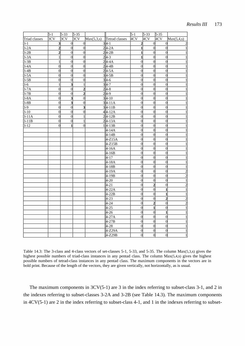
Results III 173
5-1 5-33 5-35 5-1 5-33 5-35 Triad classes 3CV 3CV 3CV Max(5,3,s) Tetrad classes 4CV 4CV 4CV Max(5,4,s) 3-1 3 0 0 3 4-1 2 0 0 23-2A 2 0 0 2 4-2A 1 0 0 13-2B 2 0 0 2 4-2B 1 0 0 13-3A 1 0 0 2 4-3 1 0 0 13-3B 1 0 0 2 4-4A 0 0 0 13-4A 0 0 0 2 4-4B 0 0 0 13-4B 0 0 0 2 4-5A 0 0 0 13-5A 0 0 0 3 4-5B 0 0 0 13-5B 0 0 0 3 4-6 0 0 0 13-6 1 3 1 3 4-7 0 0 0 13-7A 0 0 2 2 4-8 0 0 0 13-7B 0 0 2 2 4-9 0 0 0 13-8A 0 3 0 3 4-10 0 0 0 13-8B 0 3 0 3 4-11A 0 0 0 13-9 0 0 3 3 4-11B 0 0 0 13-10 0 0 0 4 4-12A 0 0 0 13-11A 0 0 1 2 4-12B 0 0 0 13-11B 0 0 1 2 4-13A 0 0 0 13-12 0 1 0 1 4-13B 0 0 0 1 4-14A 0 0 0 1 4-14B 0 0 0 1 4-Z15A 0 0 0 1 4-Z15B 0 0 0 1 4-16A 0 0 0 1 4-16B 0 0 0 1 4-17 0 0 0 1 4-18A 0 0 0 1 4-18B 0 0 0 1 4-19A 0 0 0 2 4-19B 0 0 0 2 4-20 0 0 0 1 4-21 0 2 0 2 4-22A 0 0 1 1 4-22B 0 0 1 1 4-23 0 0 2 2 4-24 0 2 0 2 4-25 0 1 0 1 4-26 0 0 1 1 4-27A 0 0 0 1 4-27B 0 0 0 1 4-28 0 0 0 1 4-Z29A 0 0 0 1 4-Z29B 0 0 0 1
Table 14.3: The 3-class and 4-class vectors of set-classes 5-1, 5-33, and 5-35. The column Max(5,3,s) gives the highest possible numbers of triad-class instances in any pentad class. The column Max(5,4,s) gives the highest possible numbers of tetrad-class instances in any pentad class. The maximum components in the vectors are in bold print. Because of the length of the vectors, they are given vertically, not horizontally, as is usual.
The maximum components in 3CV(5-1) are 3 in the index referring to subset-class 3-1, and 2 in
the indexes referring to subset-classes 3-2A and 3-2B (see Table 14.3). The maximum components in 4CV(5-1) are 2 in the index referring to subset-class 4-1, and 1 in the indexes referring to subset-
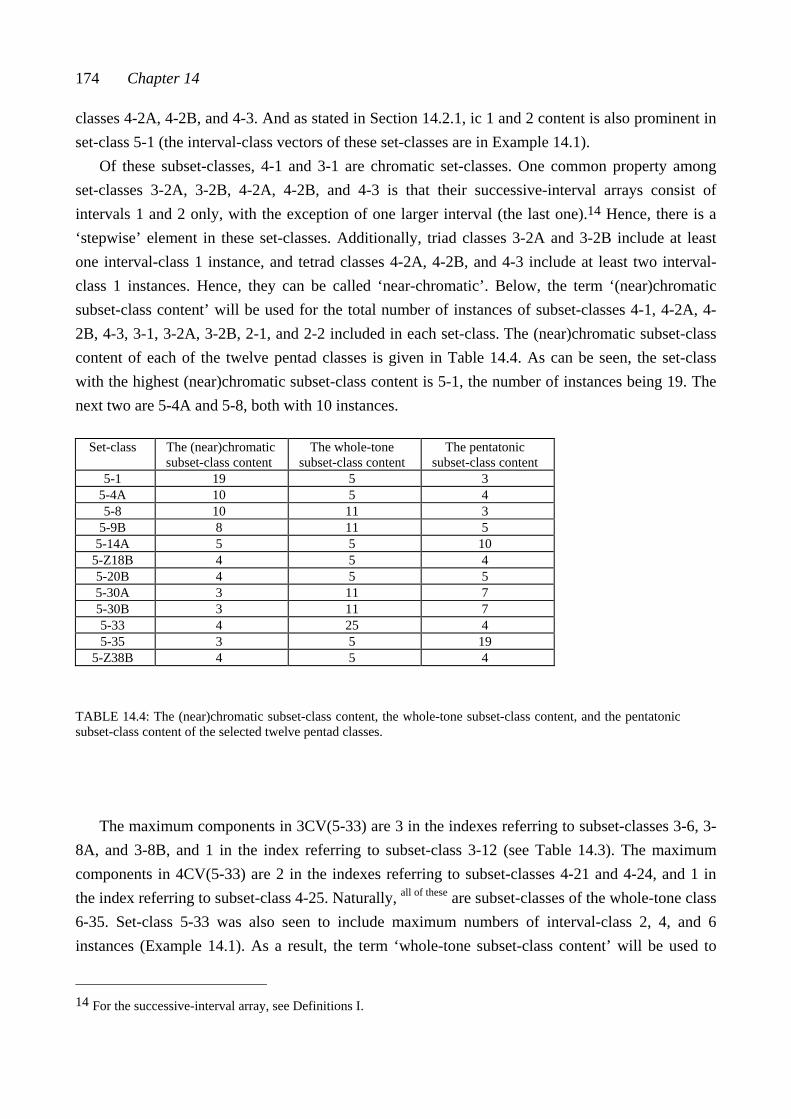
174 Chapter 14
classes 4-2A, 4-2B, and 4-3. And as stated in Section 14.2.1, ic 1 and 2 content is also prominent in set-class 5-1 (the interval-class vectors of these set-classes are in Example 14.1).
Of these subset-classes, 4-1 and 3-1 are chromatic set-classes. One common property among set-classes 3-2A, 3-2B, 4-2A, 4-2B, and 4-3 is that their successive-interval arrays consist of intervals 1 and 2 only, with the exception of one larger interval (the last one).14 Hence, there is a ‘stepwise’ element in these set-classes. Additionally, triad classes 3-2A and 3-2B include at least one interval-class 1 instance, and tetrad classes 4-2A, 4-2B, and 4-3 include at least two interval-class 1 instances. Hence, they can be called ‘near-chromatic’. Below, the term ‘(near)chromatic subset-class content’ will be used for the total number of instances of subset-classes 4-1, 4-2A, 4-2B, 4-3, 3-1, 3-2A, 3-2B, 2-1, and 2-2 included in each set-class. The (near)chromatic subset-class content of each of the twelve pentad classes is given in Table 14.4. As can be seen, the set-class with the highest (near)chromatic subset-class content is 5-1, the number of instances being 19. The next two are 5-4A and 5-8, both with 10 instances.
Set-class The (near)chromatic subset-class content
The whole-tone subset-class content
The pentatonic subset-class content
5-1 19 5 3 5-4A 10 5 4 5-8 10 11 3
5-9B 8 11 5 5-14A 5 5 10
5-Z18B 4 5 4 5-20B 4 5 5 5-30A 3 11 7 5-30B 3 11 7 5-33 4 25 4 5-35 3 5 19
5-Z38B 4 5 4 TABLE 14.4: The (near)chromatic subset-class content, the whole-tone subset-class content, and the pentatonic subset-class content of the selected twelve pentad classes.
The maximum components in 3CV(5-33) are 3 in the indexes referring to subset-classes 3-6, 3-
8A, and 3-8B, and 1 in the index referring to subset-class 3-12 (see Table 14.3). The maximum components in 4CV(5-33) are 2 in the indexes referring to subset-classes 4-21 and 4-24, and 1 in the index referring to subset-class 4-25. Naturally, all of these are subset-classes of the whole-tone class 6-35. Set-class 5-33 was also seen to include maximum numbers of interval-class 2, 4, and 6 instances (Example 14.1). As a result, the term ‘whole-tone subset-class content’ will be used to
14 For the successive-interval array, see Definitions I.
Results III 175
refer to the total number of instances of subset-classes 4-21, 4-24, 4-25, 3-6, 3-8A, 3-8B, 3-12, 2-2, 2-4, and 2-6. The whole-tone subset-class content of each of the twelve pentad classes can be seen in Table 14.4 above. Set-class 5-33 has the highest whole-tone subset-class content, the number of instances being 25. The next four set-classes are 5-8, 5-9B, 5-30A, and 5-30B, each with 11 instances.
The maximum components in 3CV(5-35) are 3 in the index referring to subset-class 3-9, and 2 in the indexes referring to subset-classes 3-7A, and 3-7B (see Table 14.3). The maximum components in 4CV(5-35) are 2 in the index referring to subset-class 4-23, and 1 in the indexes referring to subset-classes 4-22A, 4-22B, and 4-26. The common property of these subset-classes is that they do not include any chromatic components, but they do include relatively many instances of interval-classes 2 and 5. The term ‘pentatonic subset-class content’ is used when the total number of instances of subset-classes 4-22A, 4-22B, 4-23, 4-26, 3-7A, 3-7B, 3-9, 2-2, 2-5 is discussed. The pentatonic subset-class content of each of the twelve pentad classes is shown in Table 14.4 above. The set-class with the highest pentatonic subset-class content is 5-35, the number of instances being 19. The next one is 5-14A with 10 instances.
These three subset-class content categories will be used to guide the interpretation of the solutions derived from the total measures.15 As were the interval-class contents, so also the subset-class contents are quantities. Correlations are calculated between the subset-class content categories and the locations of set-classes along different dimensions to confirm the interpretations of the dimensions.
14.3.2 The three-dimensional solutions derived from REL-%, ATMEMB-%, and RECREL-%
The three-dimensional solutions derived from REL-%, ATMEMB-%, and RECREL-% were very closely related. This could be seen from the very high correlations between set-class coordinates along the three dimensions of these measures. The correlations were r = 0.98 between REL-% and ATMEMB-%, r = 0.95 between REL-% and RECREL-%, and r = 0.89 between ATMEMB-% and RECREL-%.16 Additionally, the three-dimensional solutions derived from these three measures resembled that derived from Cosθ-%. The solutions derived from ATMEMB-%, REL-%, and RECREL-% are in Figure 14.3. In this figure only the set-classes with the most remote locations along each dimension are shown. The coordinates of all set-classes are in Table A 14.4 in Appendix 5.
15 As could be seen, the interval-class content categories used in the previous sections were included in these subset-class content categories. The subset-class content categories were also closely connected to three of the factors found and interpreted by Quinn (A: ‘chromatic’, C: ‘cycle-of-fifths’, and F: ‘whole-tone’; see Footnote 10 in Section 14.2.1). 16 The correlations between these solutions were calculated in the same way explained in Section 14.2.2.
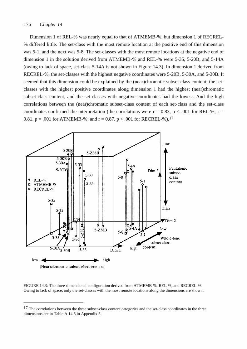
176 Chapter 14
Dimension 1 of REL-% was nearly equal to that of ATMEMB-%, but dimension 1 of RECREL-% differed little. The set-class with the most remote location at the positive end of this dimension was 5-1, and the next was 5-8. The set-classes with the most remote locations at the negative end of dimension 1 in the solution derived from ATMEMB-% and REL-% were 5-35, 5-20B, and 5-14A (owing to lack of space, set-class 5-14A is not shown in Figure 14.3). In dimension 1 derived from RECREL-%, the set-classes with the highest negative coordinates were 5-20B, 5-30A, and 5-30B. It seemed that this dimension could be explained by the (near)chromatic subset-class content; the set-classes with the highest positive coordinates along dimension 1 had the highest (near)chromatic subset-class content, and the set-classes with negative coordinates had the lowest. And the high correlations between the (near)chromatic subset-class content of each set-class and the set-class coordinates confirmed the interpretation (the correlations were r = 0.83, p < .001 for REL-%; r = 0.81, p = .001 for ATMEMB-%; and r = 0.87, p < .001 for RECREL-%).17
FIGURE 14.3: The three-dimensional configuration derived from ATMEMB-%, REL-%, and RECREL-%. Owing to lack of space, only the set-classes with the most remote locations along the dimensions are shown. 17 The correlations between the three subset-class content categories and the set-class coordinates in the three dimensions are in Table A 14.5 in Appendix 5.
Results III 177
The set-classes with the most remote locations in dimension 2 were 5-33 (alone at the negative end) and 5-4A, 5-Z38B, and 5-Z18B (at the positive end). Of these set-classes 5-Z18B is not shown in Figure 14.3 owing to lack of space. This dimension was interpreted with the help of the whole-tone subset-class content. The correlations between locations of the set-classes along this dimension and the whole-tone subset-class content of each set-class were r = -0.83 (p = .001) for REL-% and RECREL-%, and r = -0.90 (p < .001) for ATMEMB-%. These high and negative correlations indicated that the set-classes with the highest negative coordinates along dimension 2 had the highest whole-tone subset-class content.
Dimension 3 of REL-%, ATMEMB-%, and RECREL-% had set-class 5-35 alone at the negative end (the set-class with the shortest stem in Figure 14.3). There were no set-classes with remote locations at the positive end. Set-class 5-35 being so far away at its own end led to the decision that this dimension could be interpreted with the help of the pentatonic subset-class content. But the correlation between the set-class coordinates and the pentatonic subset-class contents confirmed this interpretation only in the case of RECREL-% (r = -0.82, p = .001). The correlations for REL-% and ATMEMB-% were lower (r = -0.71, p = .010 and r = -0.65, p = .026, respectively), and they indicated only some connection between these aspects. Hence, the location of set-classes along dimension 3 of REL-% and ATMEMB-% could be explained only to some extent by the pentatonic subset-class contents.
14.3.3 The three-dimensional solution derived from AvgSATSIM-%
Dimension 1 of AvgSATSIM-% had set-class 5-33 alone at the positive end. There were no set-classes with high negative coordinates in this dimension, but the set-classes with rather high negative coordinates were 5-20B, 5-14A, 5-Z38B, and 5-Z18B, respectively (see Figure 14.4, and Table A 14.6 in Appendix 5). This dimension was interpreted with the help of the whole-tone subset-class content; the set-classes with the highest positive coordinates along dimension 1 had the highest whole-tone subset-class content. The very high correlation between these aspects (r = 0.91, p < .001) confirmed the interpretation.
The set-class with the most remote location at the positive end of dimension 2 of AvgSATSIM-% was 5-1, and the next two were 5-4A and 5-8. The set-classes at the negative end were 5-30A, 5-30B, and 5-20B. This dimension (like the corresponding dimension of ATMEMB-%, REL-%, and RECREL-%) was interpreted with the help of the (near)chromatic subset-class content; set-classes with the highest coordinates along dimension 2 had the highest (near)chromatic subset-class content. The connection between these aspects was found to be very strong (r = 0.93, p < .001).

178 Chapter 14
FIGURE 14.4: The three-dimensional configuration derived from AvgSATSIM-%
Dimension 3 of AvgSATSIM-% resembled dimension 3 of ATMEMB-% and REL-%. The set-class with the most remote location at the positive end was 5-35 (the set-class with the highest stem in Figure 14.4). There were no set-classes with remote locations at the negative end of this dimension, but the set-classes with rather remote locations were 5-Z18B and 5-Z38B. This dimension was interpreted so that the set-classes with the highest positive coordinates had the highest pentatonic subset-class content. The high correlation between these aspects (r = 0.85; p < .001) supported the interpretation.
14.4 THE CONNECTION BETWEEN THE THREE-DIMENSIONAL SOLUTIONS DERIVED FROM THE CHORD-PAIR DATASET AND THE NINE PENTAD-CLASS DATASETS Dimension 1 of the three-dimensional solutions analyzed from the interval-class vector-based measures was interpreted with the help of the ic 1 and 2 content. One dimension analyzed from the total measures was interpreted with the help of the (near)chromatic subset-class content (dimension 1 analyzed from ATMEMB-%, REL-%, and RECREL-%; and dimension 2 analyzed from AvgSATSIM-%). Further, in Section 12.5.1, RDIM 1 (the ‘consonance - dissonance’ dimension
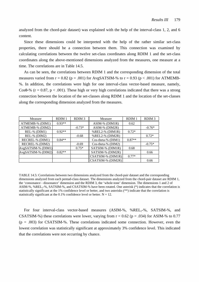
Results III 179
analyzed from the chord-pair dataset) was explained with the help of the interval-class 1, 2, and 6 content.
Since these dimensions could be interpreted with the help of the rather similar set-class properties, there should be a connection between them. This connection was examined by calculating correlations between the twelve set-class coordinates along RDIM 1 and the set-class coordinates along the above-mentioned dimensions analyzed from the measures, one measure at a time. The correlations are in Table 14.5.
As can be seen, the correlations between RDIM 1 and the corresponding dimension of the total measures varied from r = 0.82 (p = .001) for AvgSATSIM-% to r = 0.93 (p < .001) for ATMEMB-%. In addition, the correlations were high for one interval-class vector-based measure, namely, Cosθ-% (r = 0.87, p < .001). These high or very high correlations indicated that there was a strong connection between the location of the set-classes along RDIM 1 and the location of the set-classes along the corresponding dimension analyzed from the measures.
Measure RDIM 1 RDIM 3 Measure RDIM 1 RDIM 3 ATMEMB-% (DIM1) 0.93** ASIM-% (DIM1R) 0.62 ATMEMB-% (DIM2) -0.73* ASIM-% (DIM2R) -0.76*
REL-% (DIM1) 0.92** %REL2-% (DIM1R) 0.72* REL-% (DIM2) -0.68 %REL2-% (DIM2R) 0.72*
RECREL-% (DIM1) 0.84** Cos-theta-% (DIM1) 0.87** RECREL-% (DIM2) -0.69 Cos-theta-% (DIM2) -0.75*
AvgSATSIM-% (DIM1) 0.75* SATSIM-% (DIM1R) 0.68 AvgSATSIM-% (DIM2) 0.82** SATSIM-% (DIM2R) 0.66
CSATSIM-% (DIM1R) 0.77* CSATSIM-% (DIM2R) 0.66
TABLE 14.5: Correlations between two dimensions analyzed from the chord-pair dataset and the corresponding dimensions analyzed from each pentad-class dataset. The dimensions analyzed from the chord-pair dataset are RDIM 1, the ‘consonance - dissonance’ dimension and the RDIM 3, the ‘whole-tone’ dimension. The dimensions 1 and 2 of ASIM-%, %REL2-%, SATSIM-%, and CSATSIM-% have been rotated. One asterisk (*) indicates that the correlation is statistically significant at the 1% confidence level or better, and two asterisks (**) indicate that the correlation is statistically significant at the 0.1% confidence level or better. N = 12.
For four interval-class vector-based measures (ASIM-%, %REL2-%, SATSIM-%, and
CSATSIM-%) these correlations were lower, varying from r = 0.62 (p = .034) for ASIM-% to 0.77 (p = .003) for CSATSIM-%. These correlations indicated some connection. However, even the lowest correlation was statistically significant at approximately 3% confidence level. This indicated that the correlations were not occurring by chance.
180 Chapter 14
Dimension 2 of the interval-class vector-based measures was interpreted with the help of the even ic content. Dimension 1 analyzed from AvgSATSIM-% and dimension 2 analyzed from the other total measures was interpreted with the help of the whole-tone subset-class content. Additionally, RDIM 3 (the ‘whole-tone’ dimension) was explained by whole-tone attributes. To examine the connection between RDIM 3 and the mentioned dimension of each measure, correlations were calculated between the set-class coordinates along them (see Table 14.5). The correlations between RDIM 3 and the corresponding dimension of the total measures varied from r = -0.68 (p = .015) for REL-% to r = 0.75 (p = .005) for AvgSATSIM-%. The correlations for interval-class vector-based measures varied between r = 0.66 (p = .020) for SATSIM-% and CSATSIM-% and r = -0.76 (p = .004) for ASIM-%. These correlations were not very high. They indicated that there was some connection between the locations of the set-classes along RDIM 3 and the locations of the set-classes along the corresponding dimension of the measures, but differences as well. Some of these correlations were negative, indicating that the set-classes with the highest positive coordinates on RDIM 3 had the highest negative coordinates in the dimension analyzed from the measure.
The correlations between RDIM 1 and the corresponding dimension of the measures were higher for the four total measures than for the five interval-class vector-based measures. This was the case for the correlations between closeness ratings and similarity values as well (Section 12.3). The strongest connections between the analyzed dimensions were found between RDIM 1 and the corresponding dimension of ATMEMB-% (r = 0.93) and REL-% (r = 0.92), while the highest correlations between closeness ratings and similarity values were obtained for REL-% (r = 0.62), RECREL-% (r = 0.59), and ATMEMB-% (r = 0.58).
14.5 SUMMARY OF CHAPTER 14
This chapter analyzed the nine pentad-class datasets by multidimensional scaling. The three-dimensional solutions derived in these analyses turned out to be quite similar. The corresponding dimensions of each measure could be explained by rather similar, though not identical, factors. These factors were quantitative properties of set-classes. They were interval-class or subset-class content categories and were interpreted as ‘ic 1 and 2 content’ or ‘(near)chromatic’, ‘even ic content’ or ‘whole-tone’, and ‘ic 2 and 5 content’ or ‘pentatonic’.
The most important common feature in every solution was the remote position of set-classes 5-1, 5-33, and 5-35 on some dimension. This feature guided the interpretation of the dimensions. The locations of the other set-classes along the dimensions did differ, but these locations did not change the basic interpretation. Yet the locations of the other set-classes had an effect on the correlations between the set-class coordinates and the interval-class or subset-class content categories.
Results III 181
As stated in Sections 14.2.1 and 14.3.1, the interval-class and subset-class instances of the three above-mentioned set-classes were unevenly distributed in the vectors of the set-classes (that is, these vectors were ‘peaked’). Additionally, in different set-classes the ‘peaks’ were located in different vector indexes.18 Hence, it seemed that the uneven distribution of the interval-class or subset-class instances in the vectors of these set-classes (the ‘peakedness’ of the vectors) was one reason for the results. This was the case even though the measures were based on different aspects and even though the calculation procedures differed from one measure to another.
The three dimensions derived from the pentad-class datasets were also compared with the three dimensions analyzed from the chord-pair dataset. Rather high or high correlations (varying from 0.62 to 0.93) were found between RDIM1, the ‘consonance - dissonance’ dimension, and the ‘(near)chromatic’ dimension. Rather high correlations (varying between 0.66 and 0.76) were found between RDIM 3, the ‘whole-tone’ dimension, and the ‘whole-tone’ dimension of the measures.
These correlations could not be interpreted to indicate that the subjects’ closeness ratings would have been based on the same factors as the measured set-class similarity. The subjects made their ratings on the basis of the chordal characteristics, for example, the degree of consonance, or the whole-tone associations of the chords. These chordal characteristics were qualitative. But the similarity measures were based on quantitative properties of the set-classes; hence, they could not be affected by any qualitative characteristics. The chords derived from set-classes with high contents of interval-classes or subset-classes of some of the mentioned categories had salient chordal characteristics – and these were heard by the subjects. In other words, the quantitative set-class properties had effects both on the measured set-class similarity and on the qualitative characteristics of chords.
18 When the calculation processes were shown in Chapter 7, the importance of the ‘peaks’ and the zero-components was discussed.
CHAPTER FIFTEEN SUMMARY AND CONCLUSIONS
In this study two empirical tests were made. In these tests the subjects rated single pentachords on nine verbal semantic scales and pentachord pairs on the scale ‘closeness - distance’. The closeness ratings were compared to similarity values calculated by nine pitch-class set-theoretical similarity measures. Additionally, the subjects’ ratings were analyzed by three different methods, namely, factor analysis, cluster analysis, and multidimensional scaling. The results of these tests are discussed in Section 15.1, and suggestions for further study are made.
This study analyzed statistically the similarity values produced by ten similarity measures in value group #3-#9/#3-#9. Additionally, multidimensional scaling analysis was applied to nine pentad-class datasets consisting of similarity values as percentiles for 66 pentad-class pairs. The results of these analyses are discussed in Section 15.2. The conclusions appear in Section 15.3.
15.1 THE CHORD-PAIR DATASET AND THE SINGLE-CHORD DATASET
In this study, a connection was found between measured set-class similarity and perceived chordal closeness. In other words, a connection was found between quantitative and qualitative aspects of similarity. The measured (or abstract) similarity is based on quantitative properties of set-classes, which indicates that the similarity measures cannot take the realisation of the pitches, that is, the chordal setting, into account in any way. While no chordal characteristics are assigned to set-class similarity, it is likely that they are important in listening experience. The results of the study showed that the qualitative characteristics of the chords were connected with the quantitative properties of the set-classes from which the chords were derived.
The connection between set-class similarity and chordal closeness was clearer in the present study than that reported in earlier studies. One reason for this was the strict control of variables of
Summary and Conclusions 183
chordal setting of the chord pairs. As stated earlier, the chords had the same width and register. The set-classes were of the same cardinality, and the chords had an equal number of pitches. Additionally, the number of common pitches in two chords of one pair was always maximised in accordance with the number of elements in the largest mutually embeddable subset-class of the two set-classes from which the chords were derived.
All these variables of chordal setting could serve as topics for further studies. It was found by Lane that the difference in the cardinality was an important factor guiding perception of closeness between two pitch sets (1997: 199). In Lane’s study the pitch sets were melodic, and thus the increasing number of pitches had an effect on the length of the test items as well. Still, it is likely that the difference in the number of pitches of two chords would also have some effect on subjects’ closeness ratings. Further studies should be made to examine how small differences in the number of pitches would affect the ratings and how dominating the effect would be. Additionally, if the width of all chords were the same and if the number of pitches varied, the ‘density’ of the chords would most likely become a factor guiding perception of chords (as stated in Section 13.1 the subjects were not able to rate the pentachords of the test constantly on the scale ‘dense - sparse’).
The number of common pitches was found to be an important factor guiding perception of closeness between two chords. It also seemed to be one connecting factor between closeness ratings and similarity values. Further studies should be made so that the number of common pitches would vary in some systematically controlled way.
When the chord-pair dataset and the single-chord dataset were analyzed, three factors were found to guide the subjects’ ratings. Two of them, the degree of estimated consonance of a chord and the chords’ associations with familiar tonal chords, were common for both datasets. The third factor revealed from the chord-pair dataset was the chords’ whole-tone associations, while the third factor revealed from the single-chord dataset was the width and register of the chords. Hence, the (possibly unconscious) factors guiding the subjects’ ratings of chords seemed to be rather similar both for single chords and for chord pairs. This was the case even though the subjects’ ratings of the test chords were gathered by two profoundly different procedures: in the chord-pair test the ratings were based on holistic and unarticulated impressions of the chords; in the single-chord test the semantic scales broke down the total impressions of the chords into nine separate verbal dimensions. This can be said to indicate that the rather similar results were due to characteristics of the test chords, and the measuring technique did not play an important role. The connection between the results of these two tests also suggested that the order of the stimuli in the tests did not strongly affect the results. Namely, it seemed unlikely that the order of the test stimuli in two different types of tests could have caused such a high connection between the test results.
The chordal characteristics that were found to guide the subjects’ estimations of chords were also explained with the help of the properties of the set-classes from which the chords were derived. The degree of estimated consonance of a chord was strongly connected with the number of instances of certain interval-classes included in the set-class. The associations with chords familiar
184 Chapter 15
from tonal tradition as well as the whole-tone associations of chords were connected with certain aspects of the interval-class or subset-class contents of the set-classes. Hence, these chordal characteristics seemed to reflect the properties of the set-classes from which the chords were derived. Yet the arrangement of the pitches, the chordal setting, was also important. As a whole, the perceivable characteristics of chords seemed to be a mixture of two factors, namely, abstract set-class properties and chordal setting. It also seemed that the relative importance of these factors varied from case to case.
The chordal characteristics and their connection with set-class properties could serve as topics for further studies. This could help the researchers to understand the importance of these factors for perception. One possibility would be to examine whether certain properties of a set-class could be hidden in the chords derived from it. For example, if there were many instances of some interval-class in a set-class, could the intervals derived from that interval-class be represented in the chord so that the character of the interval would not dominate perception? Or if a set-class had a subset-class from which some familiar tonal chord could be derived, could this familiar tonal chord be hidden in the chordal setting?
In the two tests the chords and chord pairs were played in a musically neutral way, without any musical context. As stated in the Introduction, musical context is important in listening experience. A very important and interesting topic, but a very difficult one as well, would be to study the perception of closeness within a musical context.
The subjects of the two tests were professional musicians or music students. It is possible that the results would have been different if the subjects had been non-musicians. However, it seems unlikely that results derived from non-musicians could have been more reasonable and musically interpretable than were the results obtained in the present study. For example, with non-musician subjects perhaps there would not have been such high correlations between theoretical models of consonance and the estimated degree of consonance of chords. As was noted, for example, by Plomp and Levelt (1965: 551) and by Sethares (1997: 85), many studies have shown that in tests concerning consonance or dissonance of intervals, it is difficult for musically trained subjects to distinguish between learned musical conceptions and actual perceptions.
Summary and Conclusions 185
15.2 THE THEORETICAL SIMILARITY VALUES
Statistical analyses of shares of values produced by similarity measures were made. The analyses showed that the distributions of values by the measures differed greatly from one measure to another. The results of these analyses were taken into account when the different measures and the values produced by them were compared. Because of the different kinds of distributions of values, it seemed important to take into account the relative position of a particular value in the context of all values produced by the particular measure. Consequently, the similarity values were modified into percentiles.
Similarity values as percentiles were calculated for 66 pentad-class pairs by nine similarity measures. When these nine pentad-class datasets were analyzed in Chapter 14, highly consistent results were found. It is unclear whether these results were due to the small sample of 66 pentad-class pairs, or whether the measures were, despite their seeming differences, quite similar. It seemed that especially the ‘peakedness’ of the interval-class or subset-class vectors of the set-classes was reacted to by all similarity measures in spite of the aspects on which the measures were based.
As pentad-class pairs were used in the study, the importance of the difference in cardinality of the set-classes being compared remained untested. The objective of proportionate interval-class vectors (in measure %REL2), proportionate subset-class vectors (in measure RECREL), and saturation vectors (in measures SATSIM and AvgSATSIM) would be clearer if set-classes of different cardinalities were compared. Additionally, according to Castrén (1994a: 42-43, 60-61, 86, 89), similarity values calculated by some measures (%REL2, ASIM, and ATMEMB) are strongly affected by the difference in set-class cardinalities. It is most likely that there would have been greater dissimilarities between the results from different measures if set-classes of different cardinalities had been used. Hence, further studies with larger datasets are needed if one wants to understand fully the connection between different similarity measures.
The three-dimensional solution analyzed from the chord-pair dataset was compared with the three-dimensional solutions derived from each pentad-class dataset. Strong connections were found between the ‘consonance - dissonance’ dimension analyzed from the subjects’ closeness ratings and the ‘(near)chromatic’ dimension analyzed from the total measures as well as by the interval-class vector-based measure Cosθ (Rogers 1992, 1999). Furthermore, there was some connection between the ‘whole-tone’ dimension analyzed from the subjects’ ratings and the ‘whole-tone’ dimension analyzed from the measures.
These connections did not indicate that the degree of consonance or the whole-tone quality would have been factors affecting measured set-class similarity. As already stated, the similarity measures are quantitative and cannot be affected by any chordal characteristics. Rather, these results could again be interpreted to indicate the same connection mentioned earlier: the qualitative chordal characteristics influencing the subjects’ closeness ratings were connected with the

186 Chapter 15
quantitative interval-class or subset-class properties influencing the similarity values. As already stated, the ‘peakedness’ of the vectors of three set-classes (5-1, 5-33, and 5-35) had an effect on the similarity values, while the chords derived from these set-classes had salient chordal characteristics, and these were noticed by the subjects.
15.3 CONCLUSIONS
This study showed that there is a connection between abstract set-class similarity and aurally estimated chordal closeness. Additionally, the study showed that the underlying factors guiding perceptual estimations of chords can be explained by certain abstract properties of the set-classes from which the chords are derived. For its part the study offered new knowledge for better understanding of the strategies by which subjects rate chords. In addition, the test material (pentachords and pentachord pairs) and the methods of analysis (multidimensional scaling, hierarchical clustering, and factor analysis) seemed to be appropriate for the purposes.
The study showed that the subjects used multiple factors when they made closeness ratings. Also the ratings of single chords were based on a number of simultaneous factors. A multiple-factor structure has been revealed in earlier studies as well. Additionally, a connection was found between results derived in earlier studies and results derived in the present study, even though the earlier studies did not examine pentachords and even though the experimental design of this study differed from those of earlier studies. Two of the explanatory factors, namely, the degree of estimated consonance of chords and the associations with chords familiar from tonal music, were the same as those found by Bruner (1984).1 Also Lane (1997) interpreted one of the dimensions he found by associations with familiar, tonal pitch sets. The effect of the number of common pitches, which was reported by Bruner (1984), Gibson (1993), Lane (1997), and Williamson and Mavromatis (1997), also emerged in the chord-pair test. The importance of the width of the chords has been reported earlier by Samplaski (2000).
As a whole, it seems that the subjects tended to use rather traditional guides even when they were estimating the rather nontraditional chords of the tests. It also seems that all subjects, regardless of their listening habits and years of professional studies, used the same traditional guides. The reason for this might have been the fact that all subjects had studied or were studying classical music.
Because some factors (degree of consonance, tonal associations, number of common pitches, the width of chords) have been found in many studies, it seems possible to conclude that they are commonly used as guides in the listening experience of Westerners (none of the studies has tested 1 Bruner reported the degree of consonance of the chords with the help of the total number of semitones; hence, in her report the degree of consonance did not indicate exactly the same as the degree of consonance of the chords reported in this study.

Summary and Conclusions 187
non-Western subjects). It was also found that many of these chordal characteristics were closely connected with abstract set-class properties. Additional studies will be needed to examine further the relative importance of the chordal characteristics and the set-class properties in different kinds of contexts and to examine the importance of the other factors revealed in this study.


DEFINITIONS
The list of definitions is in three parts. The first part includes concepts of pitch-class set-theory, and the second part includes concepts of statistics. The third part explains some methods of analysis.
If a word is in bold print (set-class), it is also an entry in the list of definitions.
190 Definitions I
I Pitch-class set-theory
Cardinality (#): The cardinality of a set-class is the number of elements in each of its member sets. The terms triad class (a set-class of cardinality 3), tetrad class (#4), and pentad class (#5) will be used. Cardinality-class n: All set-classes of cardinality n (#n) constitute the cardinality-class n. Chroma circle: See pitch-class circle. Comparison group #n/#m: All set-class pairs (X, Y) such that X belongs to the cardinality-class n and Y belongs to the cardinality-class m. A given pair is counted only once, hence (X, Y) = (Y, X). When n = m, a set-class is not compared to itself. (After Castrén [1994a: 5]). Component: See interval-class vector or subset-class vector. Dyad-class percentage vector (2C%V): A modification of an interval-class vector. To transform an ICV into the corresponding 2C%V, each component (xi) is divided by the sum of all components (#ICV) and multiplied by 100 (100xi/#ICV). (After Castrén [1994a: 4]). ICV (5-1) = [4 3 2 1 0 0] #ICV(5-1) = 10 2C%V (5-1) = [40 30 20 10 0 0] Embedding function (EMB): EMB(A,X) is the number of pitch-class sets in set-class A which are subsets of a given pitch-class set in set-class X. ICV: See interval-class vector. #ICV: The sum of components in an interval-class vector. Index: See interval-class vector or subset-class vector. Interval: Given successive pitch-classes x and y, the ordered pitch-class interval between them equals (y-x) mod 12.
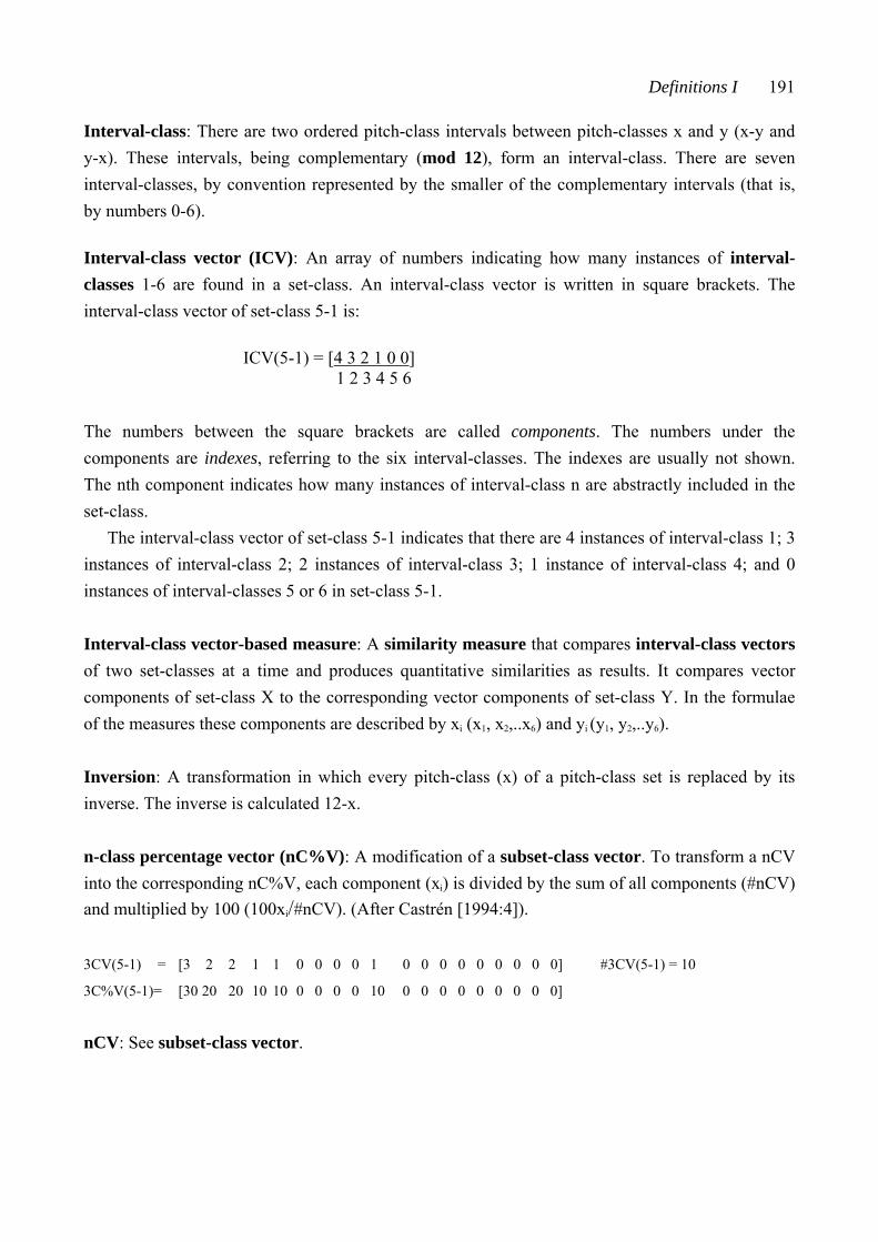
Definitions I 191
Interval-class: There are two ordered pitch-class intervals between pitch-classes x and y (x-y and y-x). These intervals, being complementary (mod 12), form an interval-class. There are seven interval-classes, by convention represented by the smaller of the complementary intervals (that is, by numbers 0-6).
Interval-class vector (ICV): An array of numbers indicating how many instances of interval-classes 1-6 are found in a set-class. An interval-class vector is written in square brackets. The interval-class vector of set-class 5-1 is: ICV(5-1) = [4 3 2 1 0 0] 1 2 3 4 5 6 The numbers between the square brackets are called components. The numbers under the components are indexes, referring to the six interval-classes. The indexes are usually not shown. The nth component indicates how many instances of interval-class n are abstractly included in the set-class.
The interval-class vector of set-class 5-1 indicates that there are 4 instances of interval-class 1; 3 instances of interval-class 2; 2 instances of interval-class 3; 1 instance of interval-class 4; and 0 instances of interval-classes 5 or 6 in set-class 5-1. Interval-class vector-based measure: A similarity measure that compares interval-class vectors of two set-classes at a time and produces quantitative similarities as results. It compares vector components of set-class X to the corresponding vector components of set-class Y. In the formulae of the measures these components are described by xi (x1, x2,..x6) and yi (y1, y2,..y6). Inversion: A transformation in which every pitch-class (x) of a pitch-class set is replaced by its inverse. The inverse is calculated 12-x. n-class percentage vector (nC%V): A modification of a subset-class vector. To transform a nCV into the corresponding nC%V, each component (xi) is divided by the sum of all components (#nCV) and multiplied by 100 (100xi/#nCV). (After Castrén [1994:4]). 3CV(5-1) = [3 2 2 1 1 0 0 0 0 1 0 0 0 0 0 0 0 0 0] #3CV(5-1) = 10
3C%V(5-1)= [30 20 20 10 10 0 0 0 0 10 0 0 0 0 0 0 0 0 0]
nCV: See subset-class vector.
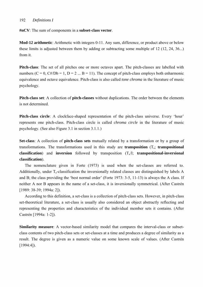
192 Definitions I
#nCV: The sum of components in a subset-class vector. Mod-12 arithmetic: Arithmetic with integers 0-11. Any sum, difference, or product above or below these limits is adjusted between them by adding or subtracting some multiple of 12 (12, 24, 36...) from it. Pitch-class: The set of all pitches one or more octaves apart. The pitch-classes are labelled with numbers (C = 0, C#/Db = 1, D = 2 ... B = 11). The concept of pitch-class employs both enharmonic equivalence and octave equivalence. Pitch-class is also called tone chroma in the literature of music psychology. Pitch-class set: A collection of pitch-classes without duplications. The order between the elements is not determined. Pitch-class circle: A clockface-shaped representation of the pitch-class universe. Every ‘hour’ represents one pitch-class. Pitch-class circle is called chroma circle in the literature of music psychology. (See also Figure 3.1 in section 3.1.1.) Set-class: A collection of pitch-class sets mutually related by a transformation or by a group of transformations. The transformations used in this study are transposition (Tn; transpositional classification) and inversion followed by transposition (Tn/I; transpositional-inversional classification).
The nomenclature given in Forte (1973) is used when the set-classes are referred to. Additionally, under Tn-classification the inversionally related classes are distinguished by labels A and B; the class providing the ‘best normal order’ (Forte 1973: 3-5, 11-13) is always the A class. If neither A nor B appears in the name of a set-class, it is inversionally symmetrical. (After Castrén [1989: 38-39; 1994a: 2]).
According to this definition, a set-class is a collection of pitch-class sets. However, in pitch-class set-theoretical literature, a set-class is usually also considered an object abstractly reflecting and representing the properties and characteristics of the individual member sets it contains. (After Castrén [1994a: 1-2]).
Similarity measure: A vector-based similarity model that compares the interval-class or subset-class contents of two pitch-class sets or set-classes at a time and produces a degree of similarity as a result. The degree is given as a numeric value on some known scale of values. (After Castrén [1994:4]).
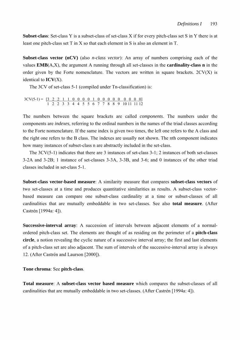
Definitions I 193
Subset-class: Set-class Y is a subset-class of set-class X if for every pitch-class set S in Y there is at least one pitch-class set T in X so that each element in S is also an element in T. Subset-class vector (nCV) (also n-class vector): An array of numbers comprising each of the values EMB(A,X), the argument A running through all set-classes in the cardinality-class n in the order given by the Forte nomenclature. The vectors are written in square brackets. 2CV(X) is identical to ICV(X).
The 3CV of set-class 5-1 (compiled under Tn-classification) is:
3CV(5-1) = [3 2 2 1 1 0 0 0 0 1 0 0 0 0 0 0 0 0 0] 1 2 2 3 3 4 4 5 5 6 7 7 8 8 9 10 11 11 12 The numbers between the square brackets are called components. The numbers under the components are indexes, referring to the ordinal numbers in the names of the triad classes according to the Forte nomenclature. If the same index is given two times, the left one refers to the A class and the right one refers to the B class. The indexes are usually not shown. The nth component indicates how many instances of subset-class n are abstractly included in the set-class.
The 3CV(5-1) indicates that there are 3 instances of set-class 3-1; 2 instances of both set-classes 3-2A and 3-2B; 1 instance of set-classes 3-3A, 3-3B, and 3-6; and 0 instances of the other triad classes included in set-class 5-1. Subset-class vector-based measure: A similarity measure that compares subset-class vectors of two set-classes at a time and produces quantitative similarities as results. A subset-class vector-based measure can compare one subset-class cardinality at a time or subset-classes of all cardinalities that are mutually embeddable in two set-classes. See also total measure. (After Castrén [1994a: 4]). Successive-interval array: A succession of intervals between adjacent elements of a normal-ordered pitch-class set. The elements are thought of as residing on the perimeter of a pitch-class circle, a notion revealing the cyclic nature of a successive interval array; the first and last elements of a pitch-class set are also adjacent. The sum of intervals of the successive-interval array is always 12. (After Castrén and Laurson [2000]). Tone chroma: See pitch-class. Total measure: A subset-class vector based measure which compares the subset-classes of all cardinalities that are mutually embeddable in two set-classes. (After Castrén [1994a: 4]).
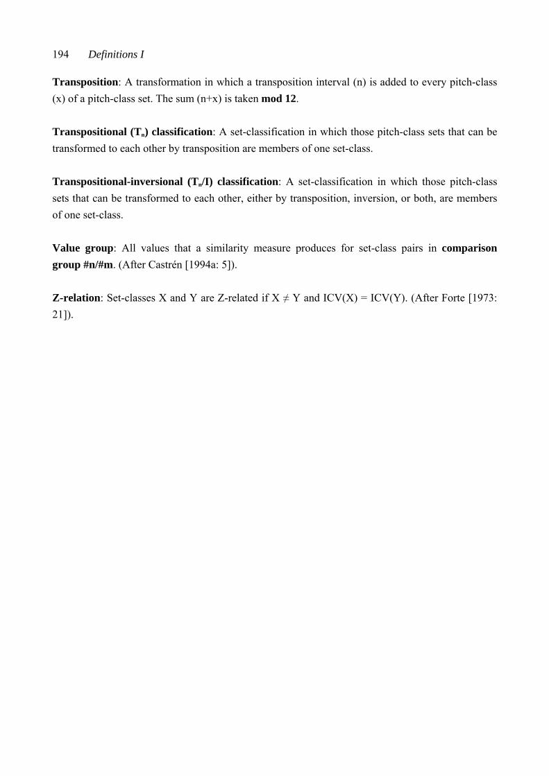
194 Definitions I
Transposition: A transformation in which a transposition interval (n) is added to every pitch-class (x) of a pitch-class set. The sum (n+x) is taken mod 12. Transpositional (Tn) classification: A set-classification in which those pitch-class sets that can be transformed to each other by transposition are members of one set-class. Transpositional-inversional (Tn/I) classification: A set-classification in which those pitch-class sets that can be transformed to each other, either by transposition, inversion, or both, are members of one set-class. Value group: All values that a similarity measure produces for set-class pairs in comparison group #n/#m. (After Castrén [1994a: 5]). Z-relation: Set-classes X and Y are Z-related if X ≠ Y and ICV(X) = ICV(Y). (After Forte [1973: 21]).
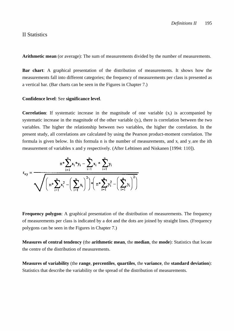
Definitions II 195
II Statistics Arithmetic mean (or average): The sum of measurements divided by the number of measurements. Bar chart: A graphical presentation of the distribution of measurements. It shows how the measurements fall into different categories; the frequency of measurements per class is presented as a vertical bar. (Bar charts can be seen in the Figures in Chapter 7.) Confidence level: See significance level. Correlation: If systematic increase in the magnitude of one variable (xi) is accompanied by systematic increase in the magnitude of the other variable (yi), there is correlation between the two variables. The higher the relationship between two variables, the higher the correlation. In the present study, all correlations are calculated by using the Pearson product-moment correlation. The formula is given below. In this formula n is the number of measurements, and xi and yi are the ith measurement of variables x and y respectively. (After Lehtinen and Niskanen [1994: 110]).
Frequency polygon: A graphical presentation of the distribution of measurements. The frequency of measurements per class is indicated by a dot and the dots are joined by straight lines. (Frequency polygons can be seen in the Figures in Chapter 7.) Measures of central tendency (the arithmetic mean, the median, the mode): Statistics that locate the centre of the distribution of measurements. Measures of variability (the range, percentiles, quartiles, the variance, the standard deviation): Statistics that describe the variability or the spread of the distribution of measurements.
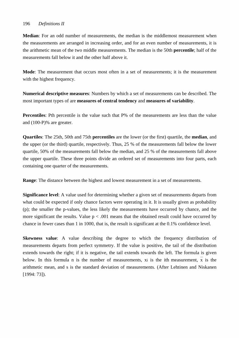
196 Definitions II
Median: For an odd number of measurements, the median is the middlemost measurement when the measurements are arranged in increasing order, and for an even number of measurements, it is the arithmetic mean of the two middle measurements. The median is the 50th percentile; half of the measurements fall below it and the other half above it. Mode: The measurement that occurs most often in a set of measurements; it is the measurement with the highest frequency. Numerical descriptive measures: Numbers by which a set of measurements can be described. The most important types of are measures of central tendency and measures of variability. Percentiles: Pth percentile is the value such that P% of the measurements are less than the value and (100-P)% are greater. Quartiles: The 25th, 50th and 75th percentiles are the lower (or the first) quartile, the median, and the upper (or the third) quartile, respectively. Thus, 25 % of the measurements fall below the lower quartile, 50% of the measurements fall below the median, and 25 % of the measurements fall above the upper quartile. These three points divide an ordered set of measurements into four parts, each containing one quarter of the measurements. Range: The distance between the highest and lowest measurement in a set of measurements. Significance level: A value used for determining whether a given set of measurements departs from what could be expected if only chance factors were operating in it. It is usually given as probability (p); the smaller the p-values, the less likely the measurements have occurred by chance, and the more significant the results. Value p < .001 means that the obtained result could have occurred by chance in fewer cases than 1 in 1000, that is, the result is significant at the 0.1% confidence level. Skewness value: A value describing the degree to which the frequency distribution of measurements departs from perfect symmetry. If the value is positive, the tail of the distribution extends towards the right; if it is negative, the tail extends towards the left. The formula is given below. In this formula n is the number of measurements, xi is the ith measurement,⎯x is the arithmetic mean, and s is the standard deviation of measurements. (After Lehtinen and Niskanen [1994: 73]).
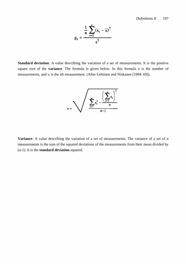
Definitions II 197
Standard deviation: A value describing the variation of a set of measurements. It is the positive square root of the variance. The formula is given below. In this formula n is the number of measurements, and xi is the ith measurement. (After Lehtinen and Niskanen [1994: 69]).
Variance: A value describing the variation of a set of measurements. The variance of a set of n measurements is the sum of the squared deviations of the measurements from their mean divided by (n-1). It is the standard deviation squared.
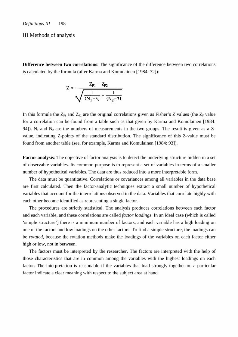
Definitions III 198
III Methods of analysis Difference between two correlations: The significance of the difference between two correlations is calculated by the formula (after Karma and Komulainen [1984: 72]):
In this formula the ZF1 and ZF2 are the original correlations given as Fisher’s Z values (the ZF value for a correlation can be found from a table such as that given by Karma and Komulainen [1984: 94]). N1 and N2 are the numbers of measurements in the two groups. The result is given as a Z-value, indicating Z-points of the standard distribution. The significance of this Z-value must be found from another table (see, for example, Karma and Komulainen [1984: 93]). Factor analysis: The objective of factor analysis is to detect the underlying structure hidden in a set of observable variables. Its common purpose is to represent a set of variables in terms of a smaller number of hypothetical variables. The data are thus reduced into a more interpretable form.
The data must be quantitative. Correlations or covariances among all variables in the data base are first calculated. Then the factor-analytic techniques extract a small number of hypothetical variables that account for the interrelations observed in the data. Variables that correlate highly with each other become identified as representing a single factor.
The procedures are strictly statistical. The analysis produces correlations between each factor and each variable, and these correlations are called factor loadings. In an ideal case (which is called ‘simple structure’) there is a minimum number of factors, and each variable has a high loading on one of the factors and low loadings on the other factors. To find a simple structure, the loadings can be rotated, because the rotation methods make the loadings of the variables on each factor either high or low, not in between.
The factors must be interpreted by the researcher. The factors are interpreted with the help of those characteristics that are in common among the variables with the highest loadings on each factor. The interpretation is reasonable if the variables that load strongly together on a particular factor indicate a clear meaning with respect to the subject area at hand.
199 Definitions III
Goodness-of-fit measures: Three goodness-of-fit measures are used in multidimensional scaling analysis. They are Young’s S-stress, Kruskal’s stress, and RSQ. Young’s S-stress and Kruskal’s stress measure how well the solution found matches the original, measured data. The stress-values range from 0 (perfect fit) to 1 (worst possible fit). RSQ measures the proportion of variance which is accounted for by the solution. RSQ values range from 0 (worst possible fit) to 1 (perfect fit). Hierarchical clustering: Cluster analysis is a procedure for classifying objects into optimally homogeneous groups on the basis of empirical ratings of characteristics of these objects. The procedure is mathematical; hence, the ratings must be quantitative. The distances between each pair of objects within the data are calculated by some distance measure (the researcher can choose the appropriate one from many possibilities), and these distances are used to cluster the objects.
In hierarchical clustering two objects that are close to each other according to the chosen distance measure are joined into a pair; then additional objects are joined to this pair. The additional objects can also form new pairs into which new objects are then joined. Two clusters can join together. Thus, in hierarchical clustering, two objects or clusters, once joined, remain together until the final step.
Cluster analysis groups the objects, but the interpretation of the clusters must be done by the researcher. The clusters are interpreted by determining which independent features seem the most discriminating between clusters. The most salient characteristics of the objects, characteristics that separate each cluster, must hence be identified. Multidimensional scaling: A procedure which uses the experimental distances between objects as its point of departure. These distances can be ‘real’ measured distances or distances reflecting how closely two entities are related psychologically (similarity estimations). The words ‘proximities’ (Shepard [1962: 126]) or ‘psychological distances’ (Carroll and Wish [1974a: 392], Kruskal and Wish [1978: 7]) are used for similarity estimations. Shepard (1962: 127) stated that since similarity is interpretable as a relation of proximity, the structure explaining the data is spatial. The spatial structure behind the distances can be revealed by multidimensional scaling. When this method is applied to data of distances, the n objects are represented geometrically by n points in m-dimensional space so that the interpoint distances correspond to the experimental distances between these objects and so that there is a minimum number of dimensions.
The number of dimensions of the spatial structure is thought of as representing the number of independent properties that are relevant for the data. The idea of multidimensionality is based on the notion that psychological distances are seldom based on only one property. Instead, many independent properties of the objects can simultaneously be used when similarity estimations are made.

Definitions III 200
Scientific judgment of the researcher is generally needed to determine the number of dimensions appropriate for the data. The goodness-of-fit measures also give some help in determining the number of dimensions. The goodness-of-fit values improve as dimensions are added. However, the dimensions must also be reasonable to interpret. Some of the higher dimensions may provide small improvement in the goodness-of-fit measures, but if these dimensions do not reveal any further interpretable structure, they should be excluded.
The structure revealed by multidimensional scaling must be interpreted by the researcher. Interpretation is based on features distinguishing the objects that are at the remote ends of the dimensions. Each dimension is then named by the properties that are in common for the group of objects at either end.
Two-sample T-test: A method to test whether the arithmetic mean of a single variable for subjects in one group differs from that for subjects in another group. The result is given as a significance.

APPENDIXES
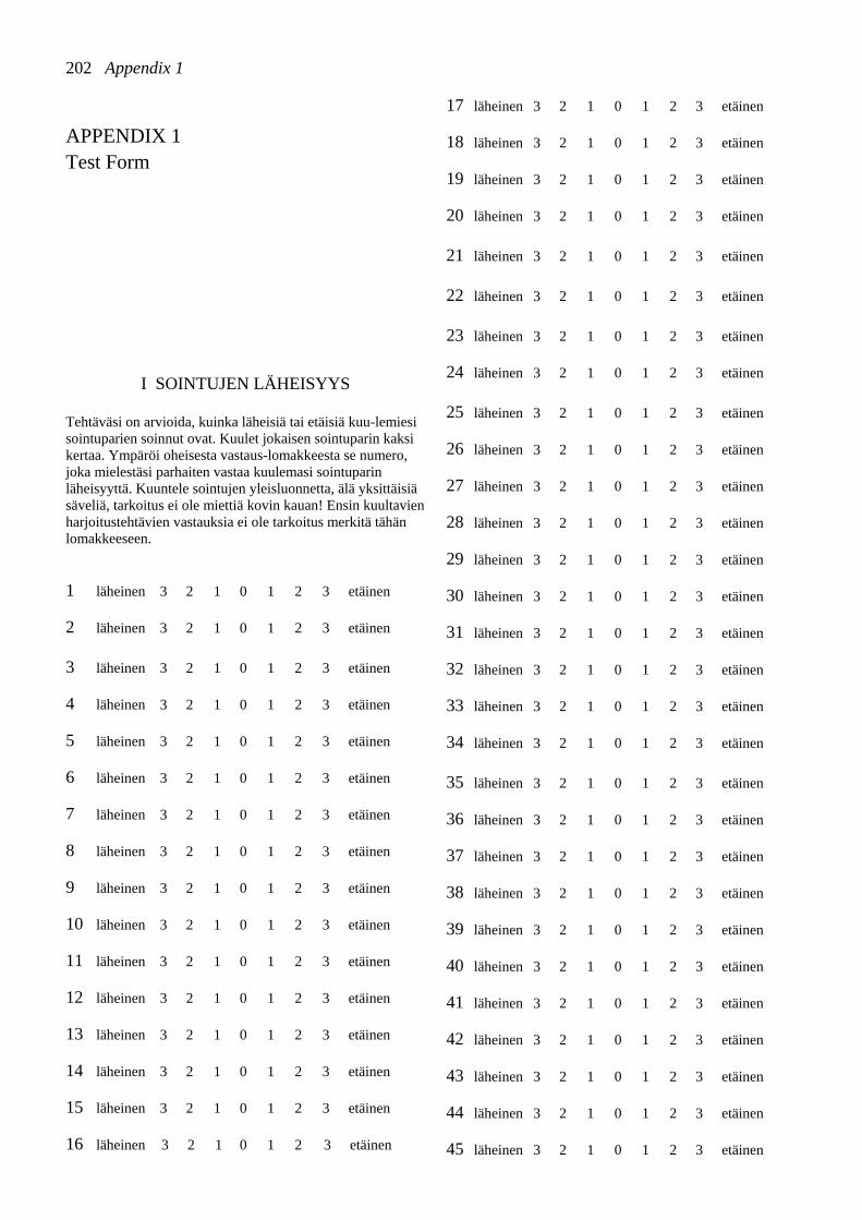
202 Appendix 1
APPENDIX 1 Test Form
I SOINTUJEN LÄHEISYYS
Tehtäväsi on arvioida, kuinka läheisiä tai etäisiä kuu-lemiesi sointuparien soinnut ovat. Kuulet jokaisen sointuparin kaksi kertaa. Ympäröi oheisesta vastaus-lomakkeesta se numero, joka mielestäsi parhaiten vastaa kuulemasi sointuparin läheisyyttä. Kuuntele sointujen yleisluonnetta, älä yksittäisiä säveliä, tarkoitus ei ole miettiä kovin kauan! Ensin kuultavien harjoitustehtävien vastauksia ei ole tarkoitus merkitä tähän lomakkeeseen. 1 läheinen 3 2 1 0 1 2 3 etäinen 2 läheinen 3 2 1 0 1 2 3 etäinen 3 läheinen 3 2 1 0 1 2 3 etäinen 4 läheinen 3 2 1 0 1 2 3 etäinen 5 läheinen 3 2 1 0 1 2 3 etäinen 6 läheinen 3 2 1 0 1 2 3 etäinen 7 läheinen 3 2 1 0 1 2 3 etäinen 8 läheinen 3 2 1 0 1 2 3 etäinen 9 läheinen 3 2 1 0 1 2 3 etäinen 10 läheinen 3 2 1 0 1 2 3 etäinen 11 läheinen 3 2 1 0 1 2 3 etäinen 12 läheinen 3 2 1 0 1 2 3 etäinen 13 läheinen 3 2 1 0 1 2 3 etäinen 14 läheinen 3 2 1 0 1 2 3 etäinen 15 läheinen 3 2 1 0 1 2 3 etäinen 16 läheinen 3 2 1 0 1 2 3 etäinen
17 läheinen 3 2 1 0 1 2 3 etäinen 18 läheinen 3 2 1 0 1 2 3 etäinen
19 läheinen 3 2 1 0 1 2 3 etäinen
20 läheinen 3 2 1 0 1 2 3 etäinen
21 läheinen 3 2 1 0 1 2 3 etäinen 22 läheinen 3 2 1 0 1 2 3 etäinen
23 läheinen 3 2 1 0 1 2 3 etäinen
24 läheinen 3 2 1 0 1 2 3 etäinen
25 läheinen 3 2 1 0 1 2 3 etäinen
26 läheinen 3 2 1 0 1 2 3 etäinen
27 läheinen 3 2 1 0 1 2 3 etäinen
28 läheinen 3 2 1 0 1 2 3 etäinen
29 läheinen 3 2 1 0 1 2 3 etäinen
30 läheinen 3 2 1 0 1 2 3 etäinen
31 läheinen 3 2 1 0 1 2 3 etäinen
32 läheinen 3 2 1 0 1 2 3 etäinen
33 läheinen 3 2 1 0 1 2 3 etäinen
34 läheinen 3 2 1 0 1 2 3 etäinen
35 läheinen 3 2 1 0 1 2 3 etäinen
36 läheinen 3 2 1 0 1 2 3 etäinen 37 läheinen 3 2 1 0 1 2 3 etäinen
38 läheinen 3 2 1 0 1 2 3 etäinen
39 läheinen 3 2 1 0 1 2 3 etäinen
40 läheinen 3 2 1 0 1 2 3 etäinen
41 läheinen 3 2 1 0 1 2 3 etäinen
42 läheinen 3 2 1 0 1 2 3 etäinen
43 läheinen 3 2 1 0 1 2 3 etäinen
44 läheinen 3 2 1 0 1 2 3 etäinen
45 läheinen 3 2 1 0 1 2 3 etäinen
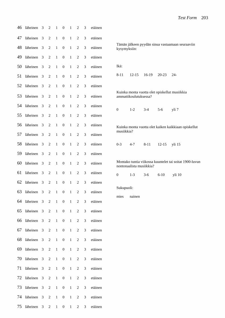
Test Form 203
46 läheinen 3 2 1 0 1 2 3 etäinen 47 läheinen 3 2 1 0 1 2 3 etäinen 48 läheinen 3 2 1 0 1 2 3 etäinen 49 läheinen 3 2 1 0 1 2 3 etäinen 50 läheinen 3 2 1 0 1 2 3 etäinen 51 läheinen 3 2 1 0 1 2 3 etäinen 52 läheinen 3 2 1 0 1 2 3 etäinen 53 läheinen 3 2 1 0 1 2 3 etäinen 54 läheinen 3 2 1 0 1 2 3 etäinen 55 läheinen 3 2 1 0 1 2 3 etäinen 56 läheinen 3 2 1 0 1 2 3 etäinen 57 läheinen 3 2 1 0 1 2 3 etäinen 58 läheinen 3 2 1 0 1 2 3 etäinen 59 läheinen 3 2 1 0 1 2 3 etäinen 60 läheinen 3 2 1 0 1 2 3 etäinen 61 läheinen 3 2 1 0 1 2 3 etäinen 62 läheinen 3 2 1 0 1 2 3 etäinen 63 läheinen 3 2 1 0 1 2 3 etäinen 64 läheinen 3 2 1 0 1 2 3 etäinen 65 läheinen 3 2 1 0 1 2 3 etäinen 66 läheinen 3 2 1 0 1 2 3 etäinen 67 läheinen 3 2 1 0 1 2 3 etäinen 68 läheinen 3 2 1 0 1 2 3 etäinen 69 läheinen 3 2 1 0 1 2 3 etäinen 70 läheinen 3 2 1 0 1 2 3 etäinen 71 läheinen 3 2 1 0 1 2 3 etäinen 72 läheinen 3 2 1 0 1 2 3 etäinen 73 läheinen 3 2 1 0 1 2 3 etäinen 74 läheinen 3 2 1 0 1 2 3 etäinen 75 läheinen 3 2 1 0 1 2 3 etäinen
Tämän jälkeen pyydän sinua vastaamaan seuraaviin kysymyksiin: Ikä: 8-11 12-15 16-19 20-23 24- Kuinka monta vuotta olet opiskellut musiikkia ammattikoulutuksessa? 0 1-2 3-4 5-6 yli 7 Kuinka monta vuotta olet kaiken kaikkiaan opiskellut musiikkia? 0-3 4-7 8-11 12-15 yli 15 Montako tuntia viikossa kuuntelet tai soitat 1900-luvun nontonaalista musiikkia? 0 1-3 3-6 6-10 yli 10 Sukupuoli: mies nainen
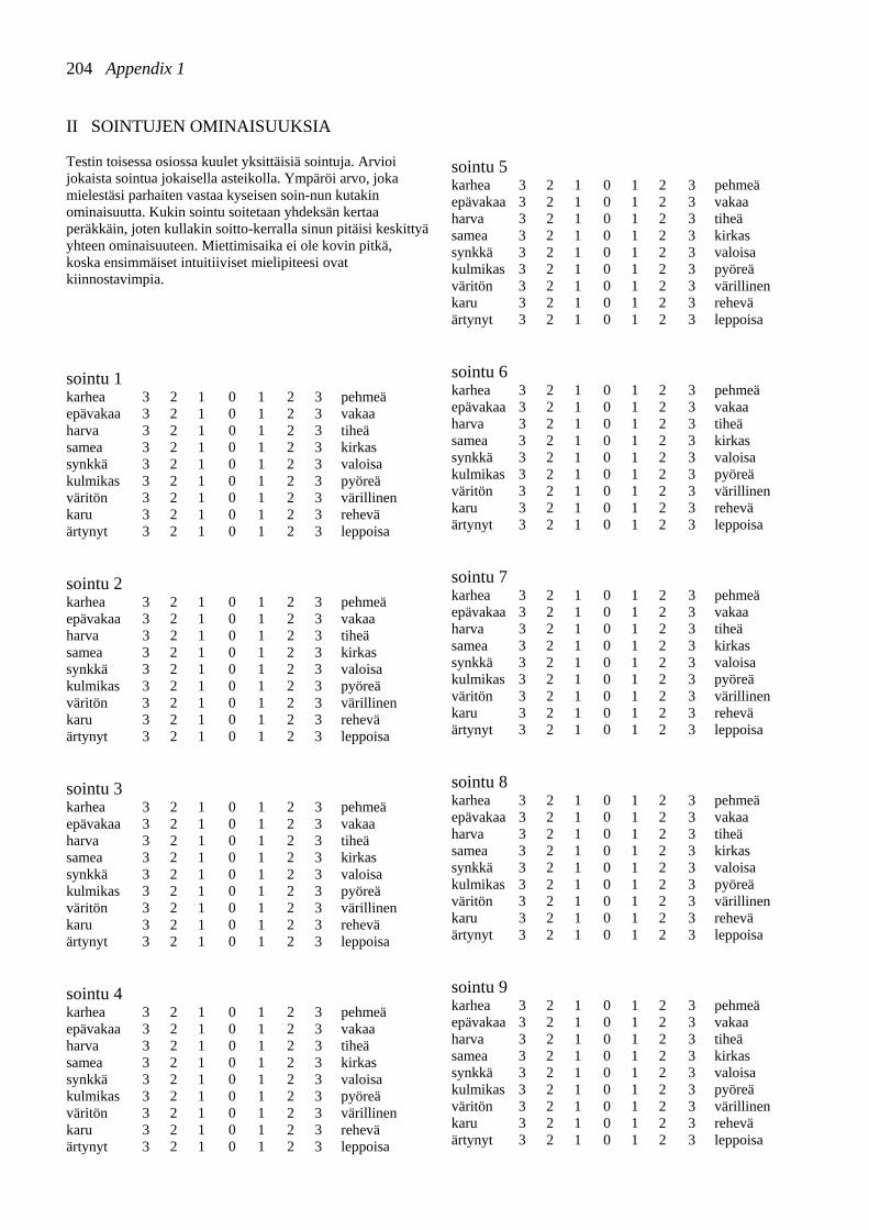
204 Appendix 1
II SOINTUJEN OMINAISUUKSIA Testin toisessa osiossa kuulet yksittäisiä sointuja. Arvioi jokaista sointua jokaisella asteikolla. Ympäröi arvo, joka mielestäsi parhaiten vastaa kyseisen soin-nun kutakin ominaisuutta. Kukin sointu soitetaan yhdeksän kertaa peräkkäin, joten kullakin soitto-kerralla sinun pitäisi keskittyä yhteen ominaisuuteen. Miettimisaika ei ole kovin pitkä, koska ensimmäiset intuitiiviset mielipiteesi ovat kiinnostavimpia. sointu 1 karhea 3 2 1 0 1 2 3 pehmeä epävakaa 3 2 1 0 1 2 3 vakaa harva 3 2 1 0 1 2 3 tiheä samea 3 2 1 0 1 2 3 kirkas synkkä 3 2 1 0 1 2 3 valoisa kulmikas 3 2 1 0 1 2 3 pyöreä väritön 3 2 1 0 1 2 3 värillinen karu 3 2 1 0 1 2 3 rehevä ärtynyt 3 2 1 0 1 2 3 leppoisa sointu 2 karhea 3 2 1 0 1 2 3 pehmeä epävakaa 3 2 1 0 1 2 3 vakaa harva 3 2 1 0 1 2 3 tiheä samea 3 2 1 0 1 2 3 kirkas synkkä 3 2 1 0 1 2 3 valoisa kulmikas 3 2 1 0 1 2 3 pyöreä väritön 3 2 1 0 1 2 3 värillinen karu 3 2 1 0 1 2 3 rehevä ärtynyt 3 2 1 0 1 2 3 leppoisa sointu 3 karhea 3 2 1 0 1 2 3 pehmeä epävakaa 3 2 1 0 1 2 3 vakaa harva 3 2 1 0 1 2 3 tiheä samea 3 2 1 0 1 2 3 kirkas synkkä 3 2 1 0 1 2 3 valoisa kulmikas 3 2 1 0 1 2 3 pyöreä väritön 3 2 1 0 1 2 3 värillinen karu 3 2 1 0 1 2 3 rehevä ärtynyt 3 2 1 0 1 2 3 leppoisa sointu 4 karhea 3 2 1 0 1 2 3 pehmeä epävakaa 3 2 1 0 1 2 3 vakaa harva 3 2 1 0 1 2 3 tiheä samea 3 2 1 0 1 2 3 kirkas synkkä 3 2 1 0 1 2 3 valoisa kulmikas 3 2 1 0 1 2 3 pyöreä väritön 3 2 1 0 1 2 3 värillinen karu 3 2 1 0 1 2 3 rehevä ärtynyt 3 2 1 0 1 2 3 leppoisa
sointu 5 karhea 3 2 1 0 1 2 3 pehmeä epävakaa 3 2 1 0 1 2 3 vakaa harva 3 2 1 0 1 2 3 tiheä samea 3 2 1 0 1 2 3 kirkas synkkä 3 2 1 0 1 2 3 valoisa kulmikas 3 2 1 0 1 2 3 pyöreä väritön 3 2 1 0 1 2 3 värillinen karu 3 2 1 0 1 2 3 rehevä ärtynyt 3 2 1 0 1 2 3 leppoisa sointu 6 karhea 3 2 1 0 1 2 3 pehmeä epävakaa 3 2 1 0 1 2 3 vakaa harva 3 2 1 0 1 2 3 tiheä samea 3 2 1 0 1 2 3 kirkas synkkä 3 2 1 0 1 2 3 valoisa kulmikas 3 2 1 0 1 2 3 pyöreä väritön 3 2 1 0 1 2 3 värillinen karu 3 2 1 0 1 2 3 rehevä ärtynyt 3 2 1 0 1 2 3 leppoisa sointu 7 karhea 3 2 1 0 1 2 3 pehmeä epävakaa 3 2 1 0 1 2 3 vakaa harva 3 2 1 0 1 2 3 tiheä samea 3 2 1 0 1 2 3 kirkas synkkä 3 2 1 0 1 2 3 valoisa kulmikas 3 2 1 0 1 2 3 pyöreä väritön 3 2 1 0 1 2 3 värillinen karu 3 2 1 0 1 2 3 rehevä ärtynyt 3 2 1 0 1 2 3 leppoisa sointu 8 karhea 3 2 1 0 1 2 3 pehmeä epävakaa 3 2 1 0 1 2 3 vakaa harva 3 2 1 0 1 2 3 tiheä samea 3 2 1 0 1 2 3 kirkas synkkä 3 2 1 0 1 2 3 valoisa kulmikas 3 2 1 0 1 2 3 pyöreä väritön 3 2 1 0 1 2 3 värillinen karu 3 2 1 0 1 2 3 rehevä ärtynyt 3 2 1 0 1 2 3 leppoisa sointu 9 karhea 3 2 1 0 1 2 3 pehmeä epävakaa 3 2 1 0 1 2 3 vakaa harva 3 2 1 0 1 2 3 tiheä samea 3 2 1 0 1 2 3 kirkas synkkä 3 2 1 0 1 2 3 valoisa kulmikas 3 2 1 0 1 2 3 pyöreä väritön 3 2 1 0 1 2 3 värillinen karu 3 2 1 0 1 2 3 rehevä ärtynyt 3 2 1 0 1 2 3 leppoisa
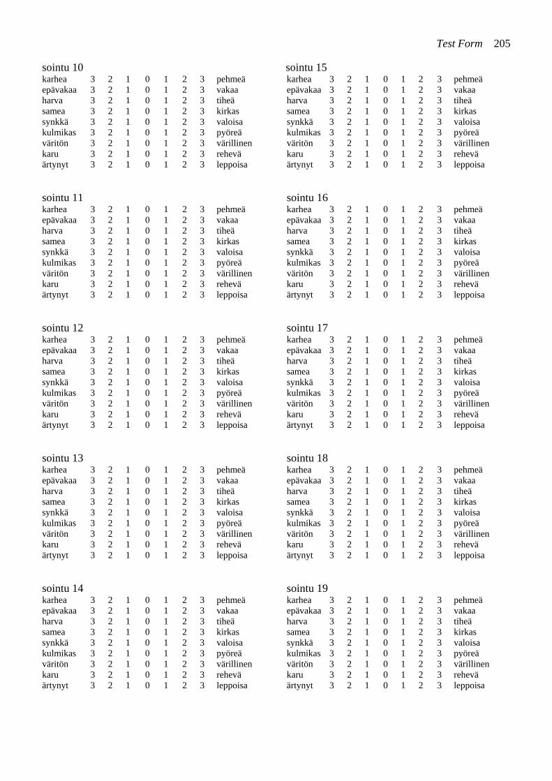
Test Form 205
sointu 10 karhea 3 2 1 0 1 2 3 pehmeä epävakaa 3 2 1 0 1 2 3 vakaa harva 3 2 1 0 1 2 3 tiheä samea 3 2 1 0 1 2 3 kirkas synkkä 3 2 1 0 1 2 3 valoisa kulmikas 3 2 1 0 1 2 3 pyöreä väritön 3 2 1 0 1 2 3 värillinen karu 3 2 1 0 1 2 3 rehevä ärtynyt 3 2 1 0 1 2 3 leppoisa sointu 11 karhea 3 2 1 0 1 2 3 pehmeä epävakaa 3 2 1 0 1 2 3 vakaa harva 3 2 1 0 1 2 3 tiheä samea 3 2 1 0 1 2 3 kirkas synkkä 3 2 1 0 1 2 3 valoisa kulmikas 3 2 1 0 1 2 3 pyöreä väritön 3 2 1 0 1 2 3 värillinen karu 3 2 1 0 1 2 3 rehevä ärtynyt 3 2 1 0 1 2 3 leppoisa sointu 12 karhea 3 2 1 0 1 2 3 pehmeä epävakaa 3 2 1 0 1 2 3 vakaa harva 3 2 1 0 1 2 3 tiheä samea 3 2 1 0 1 2 3 kirkas synkkä 3 2 1 0 1 2 3 valoisa kulmikas 3 2 1 0 1 2 3 pyöreä väritön 3 2 1 0 1 2 3 värillinen karu 3 2 1 0 1 2 3 rehevä ärtynyt 3 2 1 0 1 2 3 leppoisa sointu 13 karhea 3 2 1 0 1 2 3 pehmeä epävakaa 3 2 1 0 1 2 3 vakaa harva 3 2 1 0 1 2 3 tiheä samea 3 2 1 0 1 2 3 kirkas synkkä 3 2 1 0 1 2 3 valoisa kulmikas 3 2 1 0 1 2 3 pyöreä väritön 3 2 1 0 1 2 3 värillinen karu 3 2 1 0 1 2 3 rehevä ärtynyt 3 2 1 0 1 2 3 leppoisa sointu 14 karhea 3 2 1 0 1 2 3 pehmeä epävakaa 3 2 1 0 1 2 3 vakaa harva 3 2 1 0 1 2 3 tiheä samea 3 2 1 0 1 2 3 kirkas synkkä 3 2 1 0 1 2 3 valoisa kulmikas 3 2 1 0 1 2 3 pyöreä väritön 3 2 1 0 1 2 3 värillinen karu 3 2 1 0 1 2 3 rehevä ärtynyt 3 2 1 0 1 2 3 leppoisa
sointu 15 karhea 3 2 1 0 1 2 3 pehmeä epävakaa 3 2 1 0 1 2 3 vakaa harva 3 2 1 0 1 2 3 tiheä samea 3 2 1 0 1 2 3 kirkas synkkä 3 2 1 0 1 2 3 valoisa kulmikas 3 2 1 0 1 2 3 pyöreä väritön 3 2 1 0 1 2 3 värillinen karu 3 2 1 0 1 2 3 rehevä ärtynyt 3 2 1 0 1 2 3 leppoisa sointu 16 karhea 3 2 1 0 1 2 3 pehmeä epävakaa 3 2 1 0 1 2 3 vakaa harva 3 2 1 0 1 2 3 tiheä samea 3 2 1 0 1 2 3 kirkas synkkä 3 2 1 0 1 2 3 valoisa kulmikas 3 2 1 0 1 2 3 pyöreä väritön 3 2 1 0 1 2 3 värillinen karu 3 2 1 0 1 2 3 rehevä ärtynyt 3 2 1 0 1 2 3 leppoisa sointu 17 karhea 3 2 1 0 1 2 3 pehmeä epävakaa 3 2 1 0 1 2 3 vakaa harva 3 2 1 0 1 2 3 tiheä samea 3 2 1 0 1 2 3 kirkas synkkä 3 2 1 0 1 2 3 valoisa kulmikas 3 2 1 0 1 2 3 pyöreä väritön 3 2 1 0 1 2 3 värillinen karu 3 2 1 0 1 2 3 rehevä ärtynyt 3 2 1 0 1 2 3 leppoisa sointu 18 karhea 3 2 1 0 1 2 3 pehmeä epävakaa 3 2 1 0 1 2 3 vakaa harva 3 2 1 0 1 2 3 tiheä samea 3 2 1 0 1 2 3 kirkas synkkä 3 2 1 0 1 2 3 valoisa kulmikas 3 2 1 0 1 2 3 pyöreä väritön 3 2 1 0 1 2 3 värillinen karu 3 2 1 0 1 2 3 rehevä ärtynyt 3 2 1 0 1 2 3 leppoisa sointu 19 karhea 3 2 1 0 1 2 3 pehmeä epävakaa 3 2 1 0 1 2 3 vakaa harva 3 2 1 0 1 2 3 tiheä samea 3 2 1 0 1 2 3 kirkas synkkä 3 2 1 0 1 2 3 valoisa kulmikas 3 2 1 0 1 2 3 pyöreä väritön 3 2 1 0 1 2 3 värillinen karu 3 2 1 0 1 2 3 rehevä ärtynyt 3 2 1 0 1 2 3 leppoisa
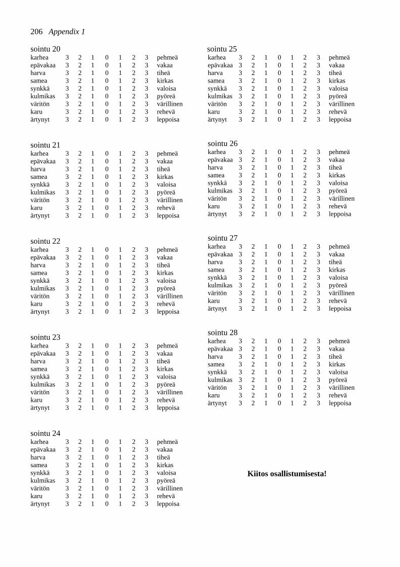
206 Appendix 1
sointu 20 karhea 3 2 1 0 1 2 3 pehmeä epävakaa 3 2 1 0 1 2 3 vakaa harva 3 2 1 0 1 2 3 tiheä samea 3 2 1 0 1 2 3 kirkas synkkä 3 2 1 0 1 2 3 valoisa kulmikas 3 2 1 0 1 2 3 pyöreä väritön 3 2 1 0 1 2 3 värillinen karu 3 2 1 0 1 2 3 rehevä ärtynyt 3 2 1 0 1 2 3 leppoisa sointu 21 karhea 3 2 1 0 1 2 3 pehmeä epävakaa 3 2 1 0 1 2 3 vakaa harva 3 2 1 0 1 2 3 tiheä samea 3 2 1 0 1 2 3 kirkas synkkä 3 2 1 0 1 2 3 valoisa kulmikas 3 2 1 0 1 2 3 pyöreä väritön 3 2 1 0 1 2 3 värillinen karu 3 2 1 0 1 2 3 rehevä ärtynyt 3 2 1 0 1 2 3 leppoisa sointu 22 karhea 3 2 1 0 1 2 3 pehmeä epävakaa 3 2 1 0 1 2 3 vakaa harva 3 2 1 0 1 2 3 tiheä samea 3 2 1 0 1 2 3 kirkas synkkä 3 2 1 0 1 2 3 valoisa kulmikas 3 2 1 0 1 2 3 pyöreä väritön 3 2 1 0 1 2 3 värillinen karu 3 2 1 0 1 2 3 rehevä ärtynyt 3 2 1 0 1 2 3 leppoisa sointu 23 karhea 3 2 1 0 1 2 3 pehmeä epävakaa 3 2 1 0 1 2 3 vakaa harva 3 2 1 0 1 2 3 tiheä samea 3 2 1 0 1 2 3 kirkas synkkä 3 2 1 0 1 2 3 valoisa kulmikas 3 2 1 0 1 2 3 pyöreä väritön 3 2 1 0 1 2 3 värillinen karu 3 2 1 0 1 2 3 rehevä ärtynyt 3 2 1 0 1 2 3 leppoisa sointu 24 karhea 3 2 1 0 1 2 3 pehmeä epävakaa 3 2 1 0 1 2 3 vakaa harva 3 2 1 0 1 2 3 tiheä samea 3 2 1 0 1 2 3 kirkas synkkä 3 2 1 0 1 2 3 valoisa kulmikas 3 2 1 0 1 2 3 pyöreä väritön 3 2 1 0 1 2 3 värillinen karu 3 2 1 0 1 2 3 rehevä ärtynyt 3 2 1 0 1 2 3 leppoisa
sointu 25 karhea 3 2 1 0 1 2 3 pehmeä epävakaa 3 2 1 0 1 2 3 vakaa harva 3 2 1 0 1 2 3 tiheä samea 3 2 1 0 1 2 3 kirkas synkkä 3 2 1 0 1 2 3 valoisa kulmikas 3 2 1 0 1 2 3 pyöreä väritön 3 2 1 0 1 2 3 värillinen karu 3 2 1 0 1 2 3 rehevä ärtynyt 3 2 1 0 1 2 3 leppoisa sointu 26 karhea 3 2 1 0 1 2 3 pehmeä epävakaa 3 2 1 0 1 2 3 vakaa harva 3 2 1 0 1 2 3 tiheä samea 3 2 1 0 1 2 3 kirkas synkkä 3 2 1 0 1 2 3 valoisa kulmikas 3 2 1 0 1 2 3 pyöreä väritön 3 2 1 0 1 2 3 värillinen karu 3 2 1 0 1 2 3 rehevä ärtynyt 3 2 1 0 1 2 3 leppoisa sointu 27 karhea 3 2 1 0 1 2 3 pehmeä epävakaa 3 2 1 0 1 2 3 vakaa harva 3 2 1 0 1 2 3 tiheä samea 3 2 1 0 1 2 3 kirkas synkkä 3 2 1 0 1 2 3 valoisa kulmikas 3 2 1 0 1 2 3 pyöreä väritön 3 2 1 0 1 2 3 värillinen karu 3 2 1 0 1 2 3 rehevä ärtynyt 3 2 1 0 1 2 3 leppoisa sointu 28 karhea 3 2 1 0 1 2 3 pehmeä epävakaa 3 2 1 0 1 2 3 vakaa harva 3 2 1 0 1 2 3 tiheä samea 3 2 1 0 1 2 3 kirkas synkkä 3 2 1 0 1 2 3 valoisa kulmikas 3 2 1 0 1 2 3 pyöreä väritön 3 2 1 0 1 2 3 värillinen karu 3 2 1 0 1 2 3 rehevä ärtynyt 3 2 1 0 1 2 3 leppoisa
Kiitos osallistumisesta!
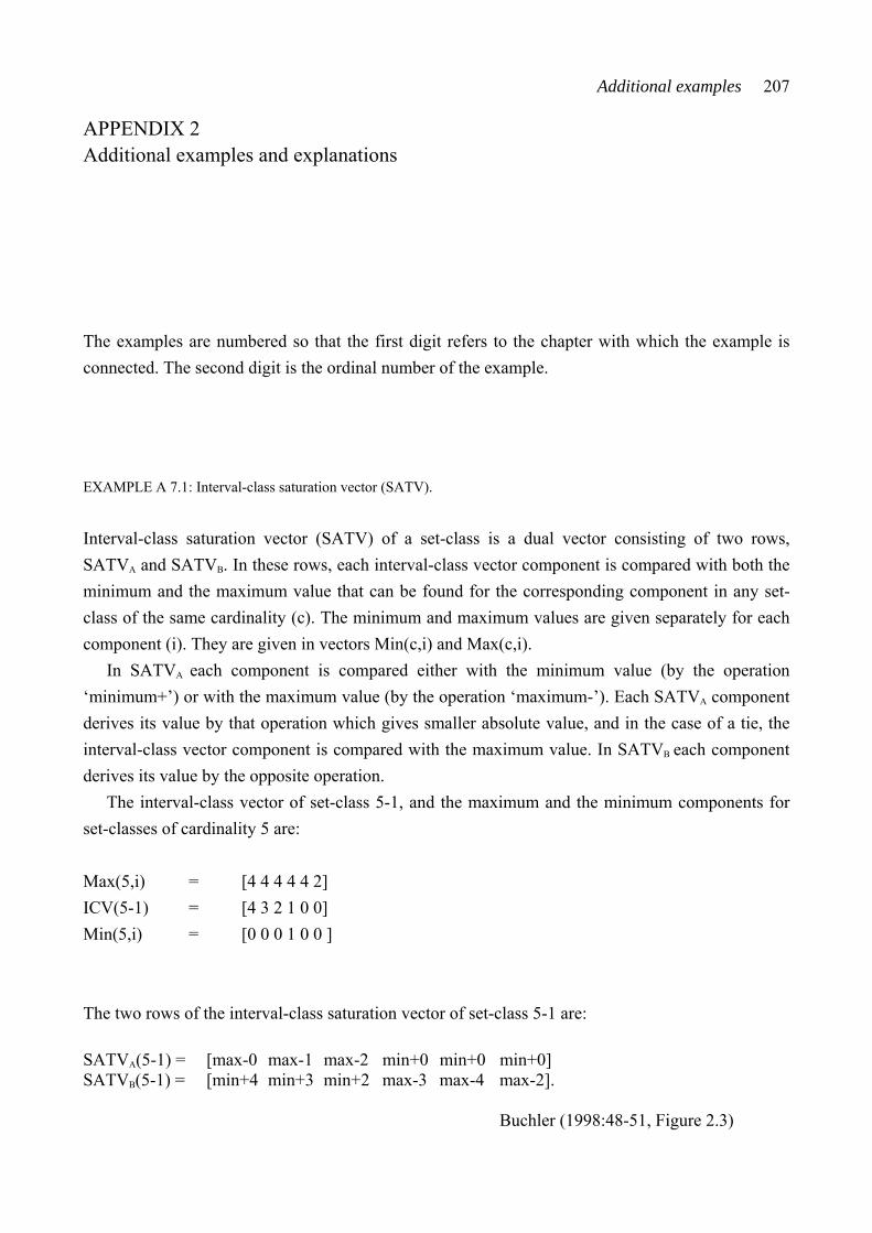
Additional examples 207
APPENDIX 2 Additional examples and explanations The examples are numbered so that the first digit refers to the chapter with which the example is connected. The second digit is the ordinal number of the example. EXAMPLE A 7.1: Interval-class saturation vector (SATV).
Interval-class saturation vector (SATV) of a set-class is a dual vector consisting of two rows, SATVA and SATVB. In these rows, each interval-class vector component is compared with both the minimum and the maximum value that can be found for the corresponding component in any set-class of the same cardinality (c). The minimum and maximum values are given separately for each component (i). They are given in vectors Min(c,i) and Max(c,i).
In SATVA each component is compared either with the minimum value (by the operation ‘minimum+’) or with the maximum value (by the operation ‘maximum-’). Each SATVA component derives its value by that operation which gives smaller absolute value, and in the case of a tie, the interval-class vector component is compared with the maximum value. In SATVB each component derives its value by the opposite operation.
The interval-class vector of set-class 5-1, and the maximum and the minimum components for set-classes of cardinality 5 are: Max(5,i) = [4 4 4 4 4 2] ICV(5-1) = [4 3 2 1 0 0] Min(5,i) = [0 0 0 1 0 0 ] The two rows of the interval-class saturation vector of set-class 5-1 are: SATVA(5-1) = [max-0 max-1 max-2 min+0 min+0 min+0] SATVB(5-1) = [min+4 min+3 min+2 max-3 max-4 max-2]. Buchler (1998:48-51, Figure 2.3)
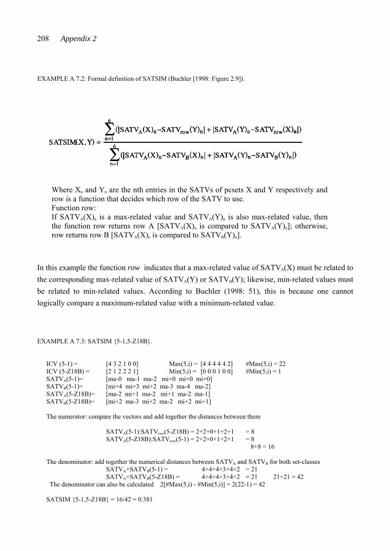
208 Appendix 2
EXAMPLE A 7.2: Formal definition of SATSIM (Buchler [1998: Figure 2.9]).
Where Xn and Yn are the nth entries in the SATVs of pcsets X and Y respectively and row is a function that decides which row of the SATV to use. Function row: If SATVA(X)n is a max-related value and SATVA(Y)n is also max-related value, then the function row returns row A [SATVA(X)n is compared to SATVA(Y)n]; otherwise, row returns row B [SATVA(X)n is compared to SATVB(Y)n].
In this example the function row indicates that a max-related value of SATVA(X) must be related to the corresponding max-related value of SATVA(Y) or SATVB(Y); likewise, min-related values must be related to min-related values. According to Buchler (1998: 51), this is because one cannot logically compare a maximum-related value with a minimum-related value. EXAMPLE A 7.3: SATSIM {5-1,5-Z18B}.
ICV (5-1) = [4 3 2 1 0 0] Max(5,i) = [4 4 4 4 4 2] #Max(5,i) = 22 ICV (5-Z18B) = [2 1 2 2 2 1] Min(5,i) = [0 0 0 1 0 0] #Min(5,i) = 1 SATVA(5-1)= [ma-0 ma-1 ma-2 mi+0 mi+0 mi+0] SATVB(5-1)= [mi+4 mi+3 mi+2 ma-3 ma-4 ma-2] SATVA(5-Z18B)= [ma-2 mi+1 ma-2 mi+1 ma-2 ma-1] SATVB(5-Z18B)= [mi+2 ma-3 mi+2 ma-2 mi+2 mi+1] The numerator: compare the vectors and add together the distances between them SATVA(5-1):SATVrow(5-Z18B) = 2+2+0+1+2+1 = 8 SATVA(5-Z18B):SATVrow(5-1) = 2+2+0+1+2+1 = 8 8+8 = 16 The denominator: add together the numerical distances between SATVA and SATVB for both set-classes SATVA+SATVB(5-1) = 4+4+4+3+4+2 = 21 SATVA+SATVB(5-Z18B) = 4+4+4+3+4+2 = 21 21+21 = 42 The denominator can also be calculated 2[#Max(5,i) - #Min(5,i)] = 2(22-1) = 42 SATSIM {5-1,5-Z18B} = 16/42 = 0.381
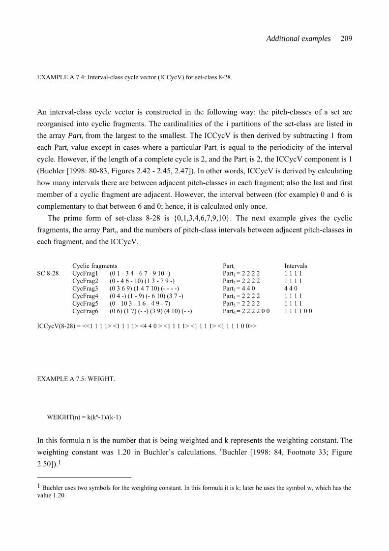
Additional examples 209
EXAMPLE A 7.4: Interval-class cycle vector (ICCycV) for set-class 8-28.
An interval-class cycle vector is constructed in the following way: the pitch-classes of a set are reorganised into cyclic fragments. The cardinalities of the i partitions of the set-class are listed in the array Parti from the largest to the smallest. The ICCycV is then derived by subtracting 1 from each Parti value except in cases where a particular Parti is equal to the periodicity of the interval cycle. However, if the length of a complete cycle is 2, and the Parti is 2, the ICCycV component is 1 (Buchler [1998: 80-83, Figures 2.42 - 2.45, 2.47]). In other words, ICCycV is derived by calculating how many intervals there are between adjacent pitch-classes in each fragment; also the last and first member of a cyclic fragment are adjacent. However, the interval between (for example) 0 and 6 is complementary to that between 6 and 0; hence, it is calculated only once.
The prime form of set-class 8-28 is {0,1,3,4,6,7,9,10}. The next example gives the cyclic fragments, the array Parti, and the numbers of pitch-class intervals between adjacent pitch-classes in each fragment, and the ICCycV. Cyclic fragments Parti Intervals SC 8-28 CycFrag1 (0 1 - 3 4 - 6 7 - 9 10 -) Part1 = 2 2 2 2 1 1 1 1 CycFrag2 (0 - 4 6 - 10) (1 3 - 7 9 -) Part2 = 2 2 2 2 1 1 1 1 CycFrag3 (0 3 6 9) (1 4 7 10) (- - - -) Part3 = 4 4 0 4 4 0 CycFrag4 (0 4 -) (1 - 9) (- 6 10) (3 7 -) Part4 = 2 2 2 2 1 1 1 1 CycFrag5 (0 - 10 3 - 1 6 - 4 9 - 7) Part5 = 2 2 2 2 1 1 1 1 CycFrag6 (0 6) (1 7) (- -) (3 9) (4 10) (- -) Part6 = 2 2 2 2 0 0 1 1 1 1 0 0 ICCycV(8-28) = <<1 1 1 1> <1 1 1 1> <4 4 0 > <1 1 1 1> <1 1 1 1> <1 1 1 1 0 0>>
EXAMPLE A 7.5: WEIGHT.
WEIGHT(n) = k(kn-1)/(k-1)
In this formula n is the number that is being weighted and k represents the weighting constant. The weighting constant was 1.20 in Buchler’s calculations. (Buchler [1998: 84, Footnote 33; Figure 2.50]).1 1 Buchler uses two symbols for the weighting constant. In this formula it is k; later he uses the symbol w, which has the value 1.20.
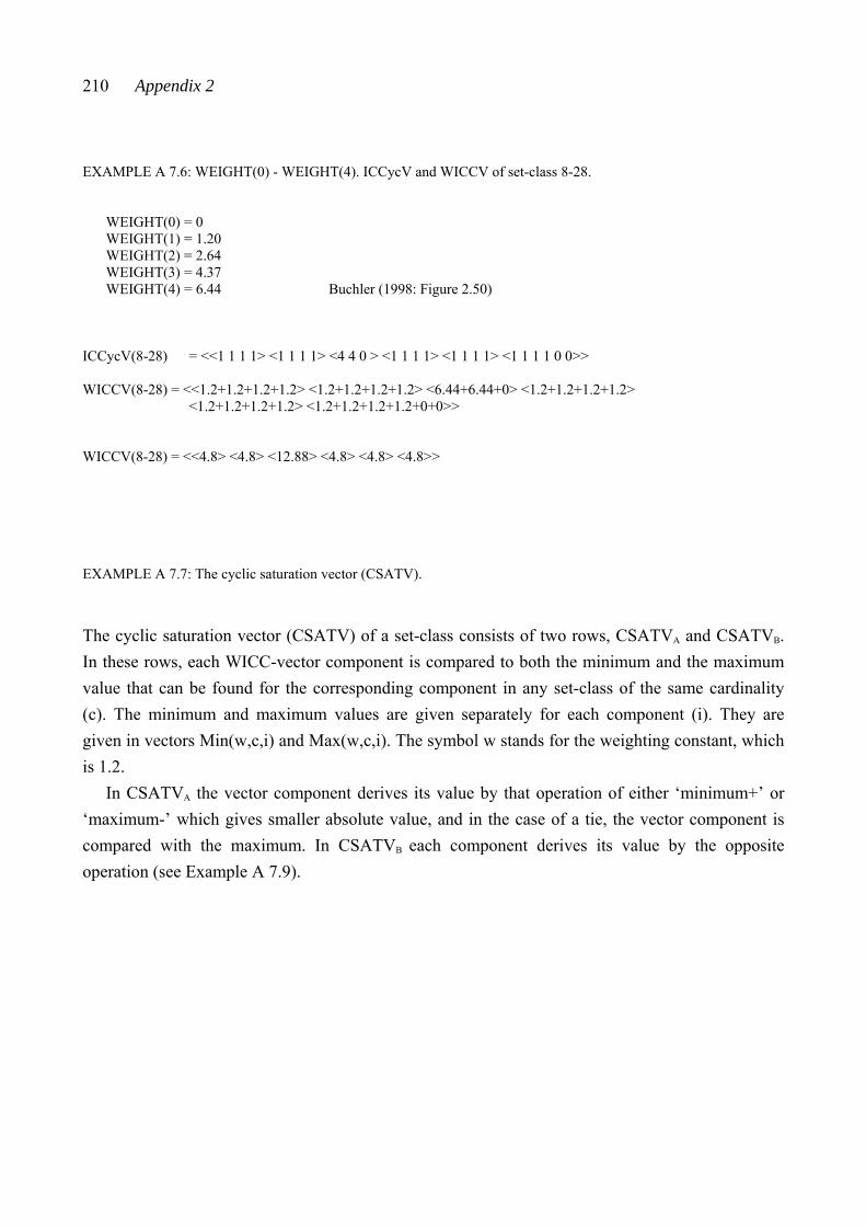
210 Appendix 2
EXAMPLE A 7.6: WEIGHT(0) - WEIGHT(4). ICCycV and WICCV of set-class 8-28.
WEIGHT(0) = 0 WEIGHT(1) = 1.20 WEIGHT(2) = 2.64 WEIGHT(3) = 4.37 WEIGHT(4) = 6.44 Buchler (1998: Figure 2.50)
ICCycV(8-28) = <<1 1 1 1> <1 1 1 1> <4 4 0 > <1 1 1 1> <1 1 1 1> <1 1 1 1 0 0>> WICCV(8-28) = <<1.2+1.2+1.2+1.2> <1.2+1.2+1.2+1.2> <6.44+6.44+0> <1.2+1.2+1.2+1.2> <1.2+1.2+1.2+1.2> <1.2+1.2+1.2+1.2+0+0>> WICCV(8-28) = <<4.8> <4.8> <12.88> <4.8> <4.8> <4.8>> EXAMPLE A 7.7: The cyclic saturation vector (CSATV). The cyclic saturation vector (CSATV) of a set-class consists of two rows, CSATVA and CSATVB. In these rows, each WICC-vector component is compared to both the minimum and the maximum value that can be found for the corresponding component in any set-class of the same cardinality (c). The minimum and maximum values are given separately for each component (i). They are given in vectors Min(w,c,i) and Max(w,c,i). The symbol w stands for the weighting constant, which is 1.2.
In CSATVA the vector component derives its value by that operation of either ‘minimum+’ or ‘maximum-’ which gives smaller absolute value, and in the case of a tie, the vector component is compared with the maximum. In CSATVB each component derives its value by the opposite operation (see Example A 7.9).
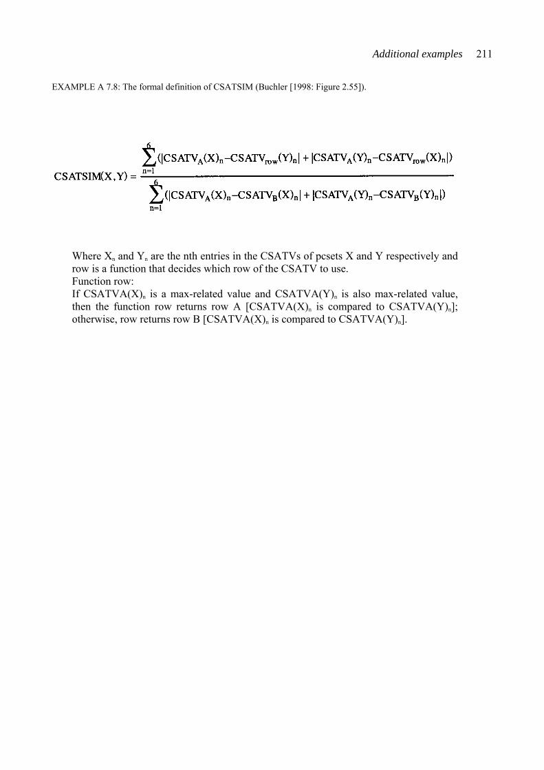
Additional examples 211
EXAMPLE A 7.8: The formal definition of CSATSIM (Buchler [1998: Figure 2.55]).
Where Xn and Yn are the nth entries in the CSATVs of pcsets X and Y respectively and row is a function that decides which row of the CSATV to use. Function row: If CSATVA(X)n is a max-related value and CSATVA(Y)n is also max-related value, then the function row returns row A [CSATVA(X)n is compared to CSATVA(Y)n]; otherwise, row returns row B [CSATVA(X)n is compared to CSATVA(Y)n].
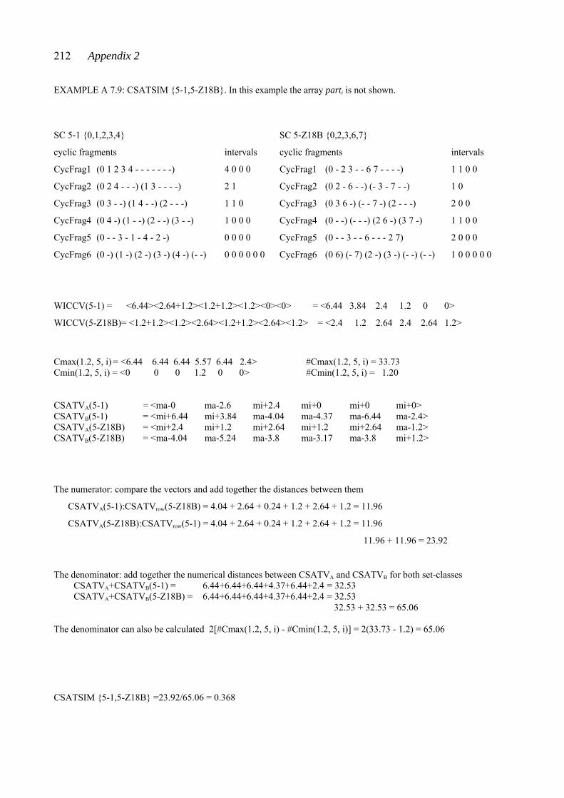
212 Appendix 2
EXAMPLE A 7.9: CSATSIM {5-1,5-Z18B}. In this example the array parti is not shown.
SC 5-1 {0,1,2,3,4} SC 5-Z18B {0,2,3,6,7}
cyclic fragments intervals cyclic fragments intervals
CycFrag1 (0 1 2 3 4 - - - - - - -) 4 0 0 0 CycFrag1 (0 - 2 3 - - 6 7 - - - -) 1 1 0 0
CycFrag2 (0 2 4 - - -) (1 3 - - - -) 2 1 CycFrag2 (0 2 - 6 - -) (- 3 - 7 - -) 1 0
CycFrag3 (0 3 - -) (1 4 - -) (2 - - -) 1 1 0 CycFrag3 (0 3 6 -) (- - 7 -) (2 - - -) 2 0 0
CycFrag4 (0 4 -) (1 - -) (2 - -) (3 - -) 1 0 0 0 CycFrag4 (0 - -) (- - -) (2 6 -) (3 7 -) 1 1 0 0
CycFrag5 (0 - - 3 - 1 - 4 - 2 -) 0 0 0 0 CycFrag5 (0 - - 3 - - 6 - - - 2 7) 2 0 0 0
CycFrag6 (0 -) (1 -) (2 -) (3 -) (4 -) (- -) 0 0 0 0 0 0 CycFrag6 (0 6) (- 7) (2 -) (3 -) (- -) (- -) 1 0 0 0 0 0
WICCV(5-1) = <6.44><2.64+1.2><1.2+1.2><1.2><0><0> = <6.44 3.84 2.4 1.2 0 0>
WICCV(5-Z18B)= <1.2+1.2><1.2><2.64><1.2+1.2><2.64><1.2> = <2.4 1.2 2.64 2.4 2.64 1.2>
Cmax(1.2, 5, i) = <6.44 6.44 6.44 5.57 6.44 2.4> #Cmax(1.2, 5, i) = 33.73 Cmin(1.2, 5, i) = <0 0 0 1.2 0 0> #Cmin(1.2, 5, i) = 1.20 CSATVA(5-1) = <ma-0 ma-2.6 mi+2.4 mi+0 mi+0 mi+0> CSATVB(5-1) = <mi+6.44 mi+3.84 ma-4.04 ma-4.37 ma-6.44 ma-2.4> CSATVA(5-Z18B) = <mi+2.4 mi+1.2 mi+2.64 mi+1.2 mi+2.64 ma-1.2> CSATVB(5-Z18B) = <ma-4.04 ma-5.24 ma-3.8 ma-3.17 ma-3.8 mi+1.2>
The numerator: compare the vectors and add together the distances between them
CSATVA(5-1):CSATVrow(5-Z18B) = 4.04 + 2.64 + 0.24 + 1.2 + 2.64 + 1.2 = 11.96
CSATVA(5-Z18B):CSATVrow(5-1) = 4.04 + 2.64 + 0.24 + 1.2 + 2.64 + 1.2 = 11.96
11.96 + 11.96 = 23.92
The denominator: add together the numerical distances between CSATVA and CSATVB for both set-classes CSATVA+CSATVB(5-1) = 6.44+6.44+6.44+4.37+6.44+2.4 = 32.53 CSATVA+CSATVB(5-Z18B) = 6.44+6.44+6.44+4.37+6.44+2.4 = 32.53
32.53 + 32.53 = 65.06 The denominator can also be calculated 2[#Cmax(1.2, 5, i) - #Cmin(1.2, 5, i)] = 2(33.73 - 1.2) = 65.06
CSATSIM {5-1,5-Z18B} =23.92/65.06 = 0.368
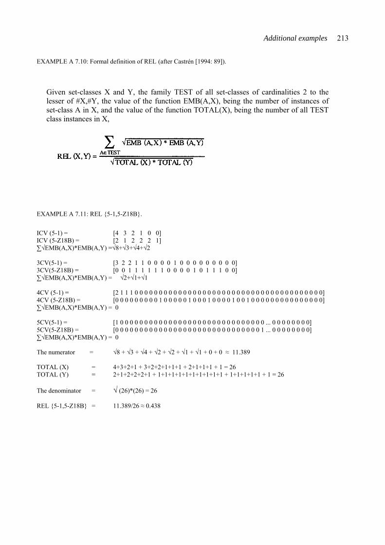
Additional examples 213
EXAMPLE A 7.10: Formal definition of REL (after Castrén [1994: 89]).
Given set-classes X and Y, the family TEST of all set-classes of cardinalities 2 to the lesser of #X,#Y, the value of the function EMB(A,X), being the number of instances of set-class A in X, and the value of the function TOTAL(X), being the number of all TEST class instances in X,
EXAMPLE A 7.11: REL {5-1,5-Z18B}.
ICV (5-1) = [4 3 2 1 0 0] ICV (5-Z18B) = [2 1 2 2 2 1] ∑√EMB(A,X)*EMB(A,Y) =√8+√3+√4+√2 3CV(5-1) = [3 2 2 1 1 0 0 0 0 1 0 0 0 0 0 0 0 0 0] 3CV(5-Z18B) = [0 0 1 1 1 1 1 1 0 0 0 0 1 0 1 1 1 0 0] ∑√EMB(A,X)*EMB(A,Y) = √2+√1+√1 4CV (5-1) = [2 1 1 1 0 0 0 0 0 0 0 0 0 0 0 0 0 0 0 0 0 0 0 0 0 0 0 0 0 0 0 0 0 0 0 0 0 0 0 0 0 0 0] 4CV (5-Z18B) = [0 0 0 0 0 0 0 0 0 1 0 0 0 0 0 1 0 0 0 1 0 0 0 0 1 0 0 1 0 0 0 0 0 0 0 0 0 0 0 0 0 0 0] ∑√EMB(A,X)*EMB(A,Y) = 0 5CV(5-1) = [1 0 0 0 0 0 0 0 0 0 0 0 0 0 0 0 0 0 0 0 0 0 0 0 0 0 0 0 0 0 0 ... 0 0 0 0 0 0 0 0] 5CV(5-Z18B) = [0 0 0 0 0 0 0 0 0 0 0 0 0 0 0 0 0 0 0 0 0 0 0 0 0 0 0 0 0 0 1 ... 0 0 0 0 0 0 0 0] ∑√EMB(A,X)*EMB(A,Y) = 0 The numerator = √8 + √3 + √4 + √2 + √2 + √1 + √1 + 0 + 0 ≈ 11.389 TOTAL (X) = 4+3+2+1 + 3+2+2+1+1+1 + 2+1+1+1 + 1 = 26 TOTAL (Y) = 2+1+2+2+2+1 + 1+1+1+1+1+1+1+1+1+1 + 1+1+1+1+1 + 1 = 26 The denominator = √ (26)*(26) = 26 REL {5-1,5-Z18B} = 11.389/26 ≈ 0.438
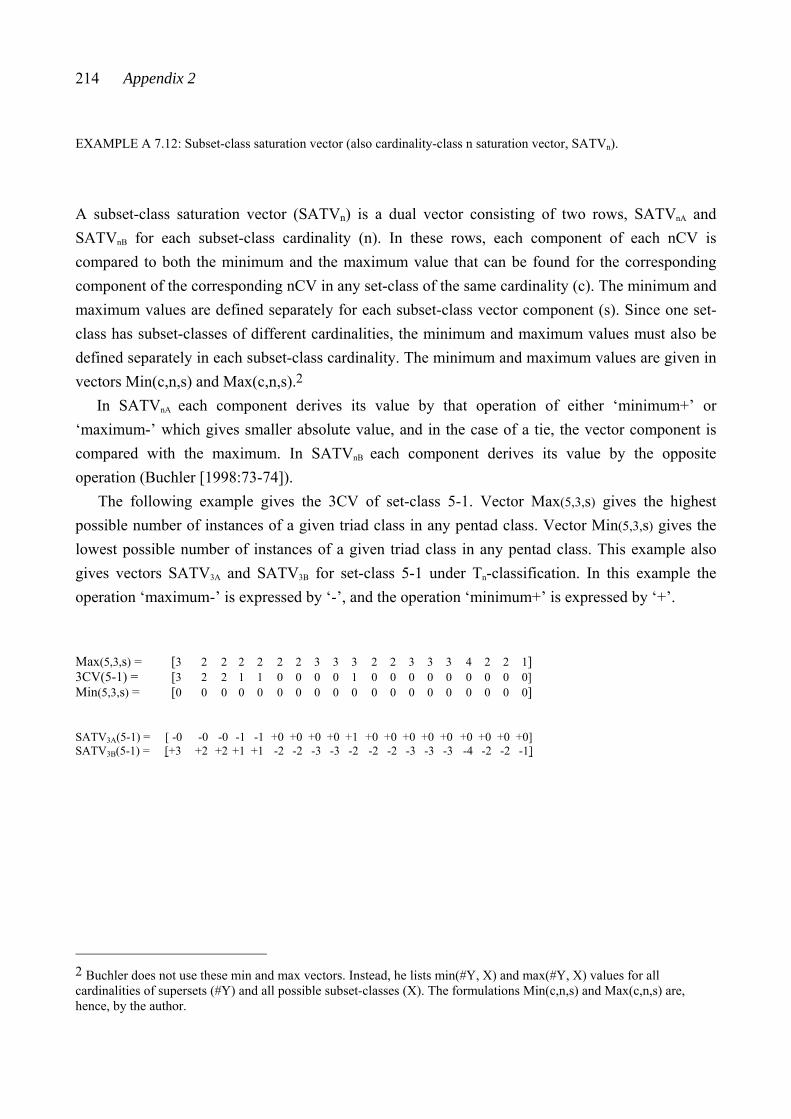
214 Appendix 2
EXAMPLE A 7.12: Subset-class saturation vector (also cardinality-class n saturation vector, SATVn).
A subset-class saturation vector (SATVn) is a dual vector consisting of two rows, SATVnA and SATVnB for each subset-class cardinality (n). In these rows, each component of each nCV is compared to both the minimum and the maximum value that can be found for the corresponding component of the corresponding nCV in any set-class of the same cardinality (c). The minimum and maximum values are defined separately for each subset-class vector component (s). Since one set-class has subset-classes of different cardinalities, the minimum and maximum values must also be defined separately in each subset-class cardinality. The minimum and maximum values are given in vectors Min(c,n,s) and Max(c,n,s).2
In SATVnA each component derives its value by that operation of either ‘minimum+’ or ‘maximum-’ which gives smaller absolute value, and in the case of a tie, the vector component is compared with the maximum. In SATVnB each component derives its value by the opposite operation (Buchler [1998:73-74]).
The following example gives the 3CV of set-class 5-1. Vector Max(5,3,s) gives the highest possible number of instances of a given triad class in any pentad class. Vector Min(5,3,s) gives the lowest possible number of instances of a given triad class in any pentad class. This example also gives vectors SATV3A and SATV3B for set-class 5-1 under Tn-classification. In this example the operation ‘maximum-’ is expressed by ‘-’, and the operation ‘minimum+’ is expressed by ‘+’.
Max(5,3,s) = [3 2 2 2 2 2 2 3 3 3 2 2 3 3 3 4 2 2 1] 3CV(5-1) = [3 2 2 1 1 0 0 0 0 1 0 0 0 0 0 0 0 0 0] Min(5,3,s) = [0 0 0 0 0 0 0 0 0 0 0 0 0 0 0 0 0 0 0] SATV3A(5-1) = [ -0 -0 -0 -1 -1 +0 +0 +0 +0 +1 +0 +0 +0 +0 +0 +0 +0 +0 +0] SATV3B(5-1) = [+3 +2 +2 +1 +1 -2 -2 -3 -3 -2 -2 -2 -3 -3 -3 -4 -2 -2 -1]
2 Buchler does not use these min and max vectors. Instead, he lists min(#Y, X) and max(#Y, X) values for all cardinalities of supersets (#Y) and all possible subset-classes (X). The formulations Min(c,n,s) and Max(c,n,s) are, hence, by the author.
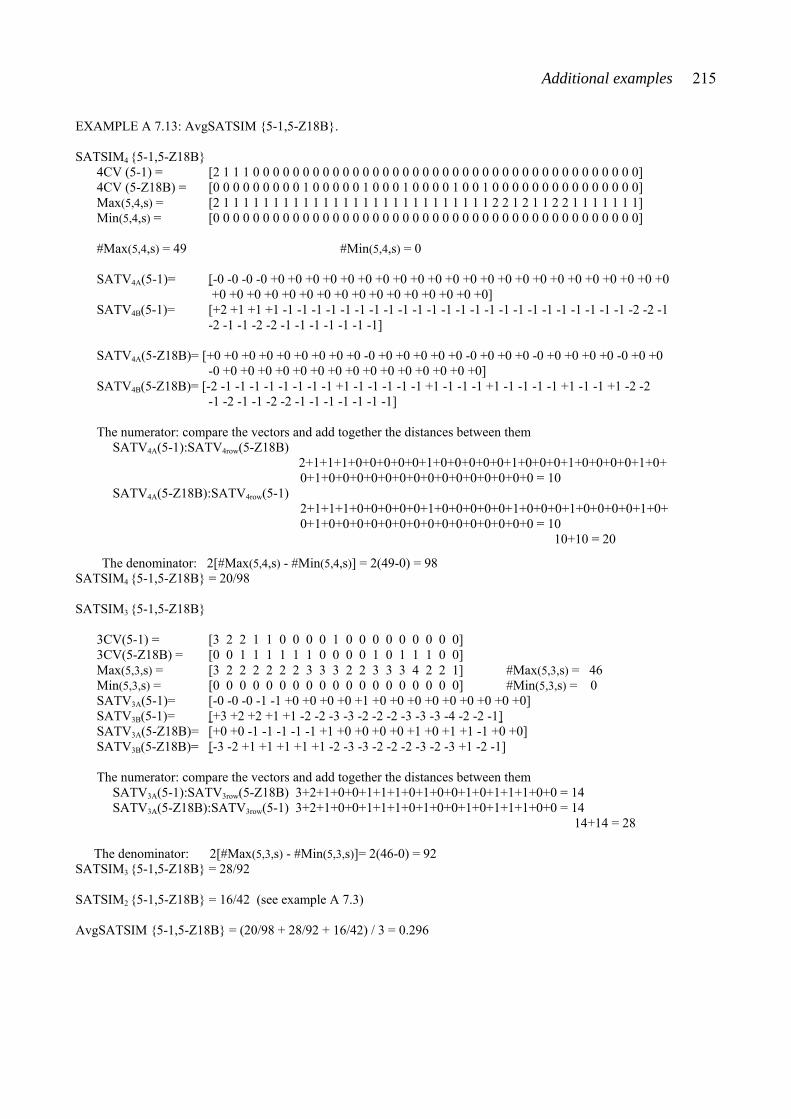
Additional examples 215
EXAMPLE A 7.13: AvgSATSIM {5-1,5-Z18B}. SATSIM4 {5-1,5-Z18B}
4CV (5-1) = [2 1 1 1 0 0 0 0 0 0 0 0 0 0 0 0 0 0 0 0 0 0 0 0 0 0 0 0 0 0 0 0 0 0 0 0 0 0 0 0 0 0 0] 4CV (5-Z18B) = [0 0 0 0 0 0 0 0 0 1 0 0 0 0 0 1 0 0 0 1 0 0 0 0 1 0 0 1 0 0 0 0 0 0 0 0 0 0 0 0 0 0 0] Max(5,4,s) = [2 1 1 1 1 1 1 1 1 1 1 1 1 1 1 1 1 1 1 1 1 1 1 1 1 1 1 1 2 2 1 2 1 1 2 2 1 1 1 1 1 1 1] Min(5,4,s) = [0 0 0 0 0 0 0 0 0 0 0 0 0 0 0 0 0 0 0 0 0 0 0 0 0 0 0 0 0 0 0 0 0 0 0 0 0 0 0 0 0 0 0] #Max(5,4,s) = 49 #Min(5,4,s) = 0 SATV4A(5-1)= [-0 -0 -0 -0 +0 +0 +0 +0 +0 +0 +0 +0 +0 +0 +0 +0 +0 +0 +0 +0 +0 +0 +0 +0 +0 +0 +0 +0 +0 +0 +0 +0 +0 +0 +0 +0 +0 +0 +0 +0 +0 +0 +0] SATV4B(5-1)= [+2 +1 +1 +1 -1 -1 -1 -1 -1 -1 -1 -1 -1 -1 -1 -1 -1 -1 -1 -1 -1 -1 -1 -1 -1 -1 -1 -1 -2 -2 -1 -2 -1 -1 -2 -2 -1 -1 -1 -1 -1 -1 -1] SATV4A(5-Z18B)= [+0 +0 +0 +0 +0 +0 +0 +0 +0 -0 +0 +0 +0 +0 +0 -0 +0 +0 +0 -0 +0 +0 +0 +0 -0 +0 +0 -0 +0 +0 +0 +0 +0 +0 +0 +0 +0 +0 +0 +0 +0 +0 +0] SATV4B(5-Z18B)= [-2 -1 -1 -1 -1 -1 -1 -1 -1 +1 -1 -1 -1 -1 -1 +1 -1 -1 -1 +1 -1 -1 -1 -1 +1 -1 -1 +1 -2 -2 -1 -2 -1 -1 -2 -2 -1 -1 -1 -1 -1 -1 -1] The numerator: compare the vectors and add together the distances between them
SATV4A(5-1):SATV4row(5-Z18B) 2+1+1+1+0+0+0+0+0+1+0+0+0+0+0+1+0+0+0+1+0+0+0+0+1+0+ 0+1+0+0+0+0+0+0+0+0+0+0+0+0+0+0+0 = 10
SATV4A(5-Z18B):SATV4row(5-1) 2+1+1+1+0+0+0+0+0+1+0+0+0+0+0+1+0+0+0+1+0+0+0+0+1+0+ 0+1+0+0+0+0+0+0+0+0+0+0+0+0+0+0+0 = 10 10+10 = 20
The denominator: 2[#Max(5,4,s) - #Min(5,4,s)] = 2(49-0) = 98 SATSIM4 {5-1,5-Z18B} = 20/98 SATSIM3 {5-1,5-Z18B}
3CV(5-1) = [3 2 2 1 1 0 0 0 0 1 0 0 0 0 0 0 0 0 0] 3CV(5-Z18B) = [0 0 1 1 1 1 1 1 0 0 0 0 1 0 1 1 1 0 0] Max(5,3,s) = [3 2 2 2 2 2 2 3 3 3 2 2 3 3 3 4 2 2 1] #Max(5,3,s) = 46 Min(5,3,s) = [0 0 0 0 0 0 0 0 0 0 0 0 0 0 0 0 0 0 0] #Min(5,3,s) = 0 SATV3A(5-1)= [-0 -0 -0 -1 -1 +0 +0 +0 +0 +1 +0 +0 +0 +0 +0 +0 +0 +0 +0] SATV3B(5-1)= [+3 +2 +2 +1 +1 -2 -2 -3 -3 -2 -2 -2 -3 -3 -3 -4 -2 -2 -1] SATV3A(5-Z18B)= [+0 +0 -1 -1 -1 -1 -1 +1 +0 +0 +0 +0 +1 +0 +1 +1 -1 +0 +0] SATV3B(5-Z18B)= [-3 -2 +1 +1 +1 +1 +1 -2 -3 -3 -2 -2 -2 -3 -2 -3 +1 -2 -1] The numerator: compare the vectors and add together the distances between them
SATV3A(5-1):SATV3row(5-Z18B) 3+2+1+0+0+1+1+1+0+1+0+0+1+0+1+1+1+0+0 = 14 SATV3A(5-Z18B):SATV3row(5-1) 3+2+1+0+0+1+1+1+0+1+0+0+1+0+1+1+1+0+0 = 14 14+14 = 28
The denominator: 2[#Max(5,3,s) - #Min(5,3,s)]= 2(46-0) = 92 SATSIM3 {5-1,5-Z18B} = 28/92
SATSIM2 {5-1,5-Z18B} = 16/42 (see example A 7.3)
AvgSATSIM {5-1,5-Z18B} = (20/98 + 28/92 + 16/42) / 3 = 0.296
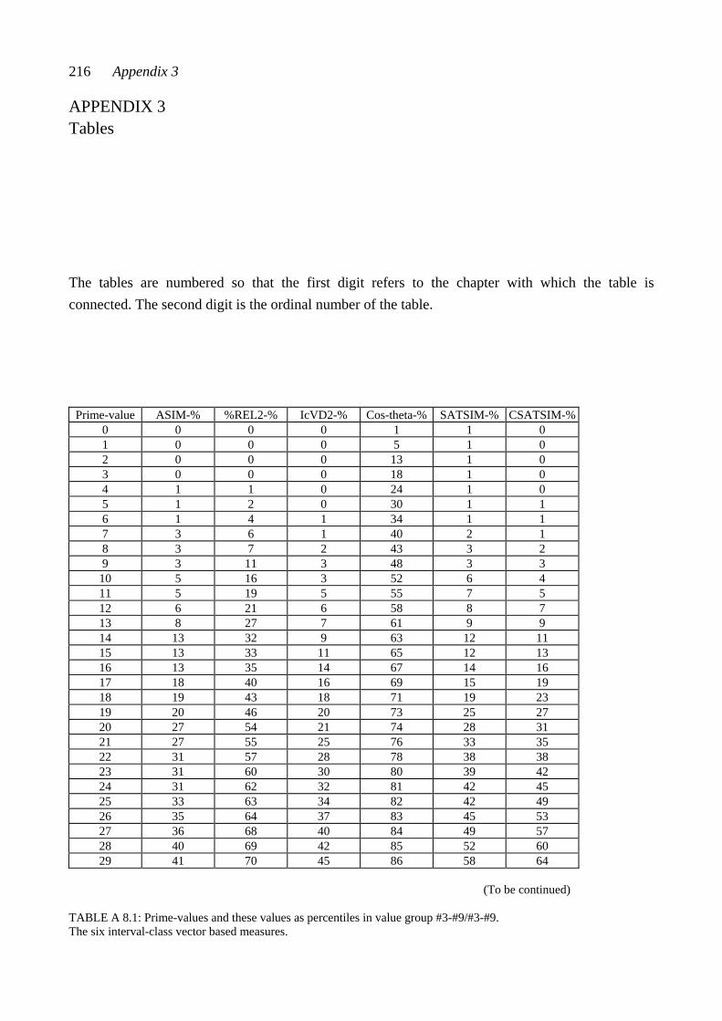
216 Appendix 3
APPENDIX 3 Tables The tables are numbered so that the first digit refers to the chapter with which the table is connected. The second digit is the ordinal number of the table.
Prime-value ASIM-% %REL2-% IcVD2-% Cos-theta-% SATSIM-% CSATSIM-% 0 0 0 0 1 1 0 1 0 0 0 5 1 0 2 0 0 0 13 1 0 3 0 0 0 18 1 0 4 1 1 0 24 1 0 5 1 2 0 30 1 1 6 1 4 1 34 1 1 7 3 6 1 40 2 1 8 3 7 2 43 3 2 9 3 11 3 48 3 3
10 5 16 3 52 6 4 11 5 19 5 55 7 5 12 6 21 6 58 8 7 13 8 27 7 61 9 9 14 13 32 9 63 12 11 15 13 33 11 65 12 13 16 13 35 14 67 14 16 17 18 40 16 69 15 19 18 19 43 18 71 19 23 19 20 46 20 73 25 27 20 27 54 21 74 28 31 21 27 55 25 76 33 35 22 31 57 28 78 38 38 23 31 60 30 80 39 42 24 31 62 32 81 42 45 25 33 63 34 82 42 49 26 35 64 37 83 45 53 27 36 68 40 84 49 57 28 40 69 42 85 52 60 29 41 70 45 86 58 64
(To be continued) TABLE A 8.1: Prime-values and these values as percentiles in value group #3-#9/#3-#9. The six interval-class vector based measures.
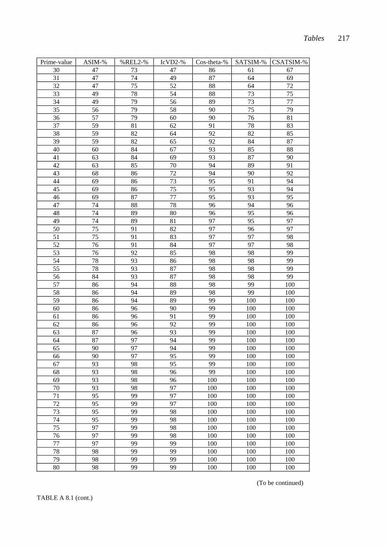
Tables 217
Prime-value ASIM-% %REL2-% IcVD2-% Cos-theta-% SATSIM-% CSATSIM-%
30 47 73 47 86 61 67 31 47 74 49 87 64 69 32 47 75 52 88 64 72 33 49 78 54 88 73 75 34 49 79 56 89 73 77 35 56 79 58 90 75 79 36 57 79 60 90 76 81 37 59 81 62 91 78 83 38 59 82 64 92 82 85 39 59 82 65 92 84 87 40 60 84 67 93 85 88 41 63 84 69 93 87 90 42 63 85 70 94 89 91 43 68 86 72 94 90 92 44 69 86 73 95 91 94 45 69 86 75 95 93 94 46 69 87 77 95 93 95 47 74 88 78 96 94 96 48 74 89 80 96 95 96 49 74 89 81 97 95 97 50 75 91 82 97 96 97 51 75 91 83 97 97 98 52 76 91 84 97 97 98 53 76 92 85 98 98 99 54 78 93 86 98 98 99 55 78 93 87 98 98 99 56 84 93 87 98 98 99 57 86 94 88 98 99 100 58 86 94 89 98 99 100 59 86 94 89 99 100 100 60 86 96 90 99 100 100 61 86 96 91 99 100 100 62 86 96 92 99 100 100 63 87 96 93 99 100 100 64 87 97 94 99 100 100 65 90 97 94 99 100 100 66 90 97 95 99 100 100 67 93 98 95 99 100 100 68 93 98 96 99 100 100 69 93 98 96 100 100 100 70 93 98 97 100 100 100 71 95 99 97 100 100 100 72 95 99 97 100 100 100 73 95 99 98 100 100 100 74 95 99 98 100 100 100 75 97 99 98 100 100 100 76 97 99 98 100 100 100 77 97 99 99 100 100 100 78 98 99 99 100 100 100 79 98 99 99 100 100 100 80 98 99 99 100 100 100
(To be continued)
TABLE A 8.1 (cont.)
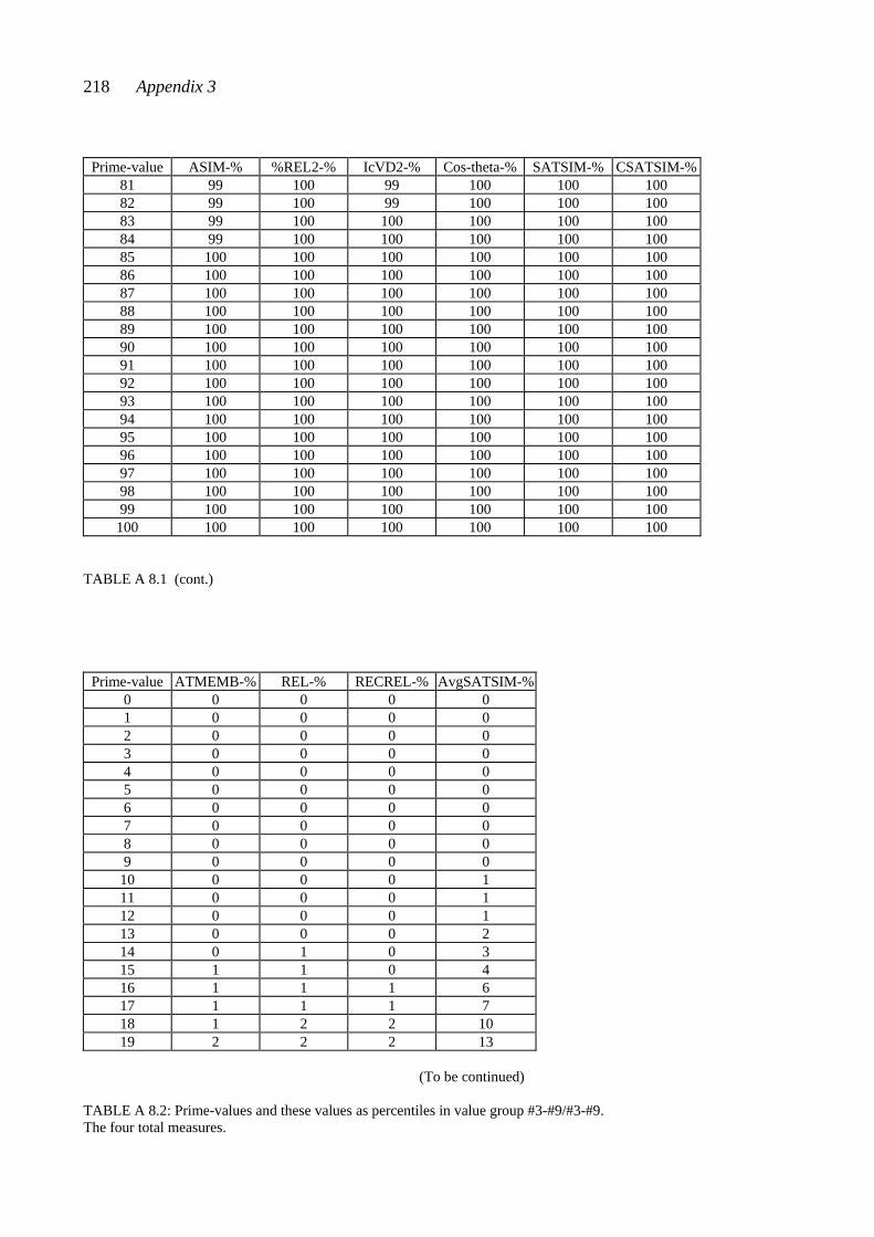
218 Appendix 3
Prime-value ASIM-% %REL2-% IcVD2-% Cos-theta-% SATSIM-% CSATSIM-%
81 99 100 99 100 100 100 82 99 100 99 100 100 100 83 99 100 100 100 100 100 84 99 100 100 100 100 100 85 100 100 100 100 100 100 86 100 100 100 100 100 100 87 100 100 100 100 100 100 88 100 100 100 100 100 100 89 100 100 100 100 100 100 90 100 100 100 100 100 100 91 100 100 100 100 100 100 92 100 100 100 100 100 100 93 100 100 100 100 100 100 94 100 100 100 100 100 100 95 100 100 100 100 100 100 96 100 100 100 100 100 100 97 100 100 100 100 100 100 98 100 100 100 100 100 100 99 100 100 100 100 100 100
100 100 100 100 100 100 100 TABLE A 8.1 (cont.)
Prime-value ATMEMB-% REL-% RECREL-% AvgSATSIM-%0 0 0 0 0 1 0 0 0 0 2 0 0 0 0 3 0 0 0 0 4 0 0 0 0 5 0 0 0 0 6 0 0 0 0 7 0 0 0 0 8 0 0 0 0 9 0 0 0 0
10 0 0 0 1 11 0 0 0 1 12 0 0 0 1 13 0 0 0 2 14 0 1 0 3 15 1 1 0 4 16 1 1 1 6 17 1 1 1 7 18 1 2 2 10 19 2 2 2 13
(To be continued) TABLE A 8.2: Prime-values and these values as percentiles in value group #3-#9/#3-#9. The four total measures.
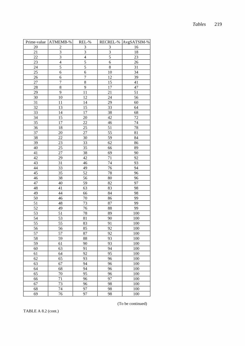
Tables 219
Prime-value ATMEMB-% REL-% RECREL-% AvgSATSIM-%
20 2 3 3 16 21 3 3 3 18 22 3 4 5 23 23 4 5 6 26 24 5 5 8 31 25 6 6 10 34 26 6 7 12 39 27 7 8 15 41 28 8 9 17 47 29 9 11 21 51 30 10 12 24 56 31 11 14 29 60 32 13 15 33 64 33 14 17 38 68 34 15 20 42 72 35 17 22 46 74 36 18 25 51 78 37 20 27 55 81 38 22 30 59 84 39 23 33 62 86 40 25 35 66 89 41 27 38 69 90 42 29 42 71 92 43 31 46 74 93 44 33 49 76 94 45 35 52 78 96 46 38 56 80 96 47 40 59 82 97 48 41 63 83 98 49 44 66 84 98 50 46 70 86 99 51 48 73 87 99 52 49 76 88 99 53 51 78 89 100 54 53 81 90 100 55 55 83 91 100 56 56 85 92 100 57 57 87 92 100 58 59 88 93 100 59 61 90 93 100 60 63 91 94 100 61 64 92 95 100 62 65 93 96 100 63 67 94 96 100 64 68 94 96 100 65 70 95 96 100 66 71 96 97 100 67 73 96 98 100 68 74 97 98 100 69 76 97 98 100
(To be continued)
TABLE A 8.2 (cont.)
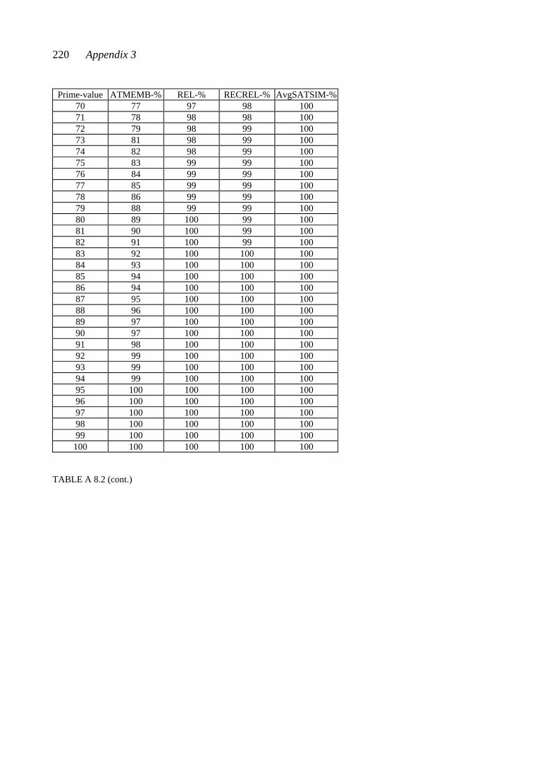
220 Appendix 3
Prime-value ATMEMB-% REL-% RECREL-% AvgSATSIM-%
70 77 97 98 100 71 78 98 98 100 72 79 98 99 100 73 81 98 99 100 74 82 98 99 100 75 83 99 99 100 76 84 99 99 100 77 85 99 99 100 78 86 99 99 100 79 88 99 99 100 80 89 100 99 100 81 90 100 99 100 82 91 100 99 100 83 92 100 100 100 84 93 100 100 100 85 94 100 100 100 86 94 100 100 100 87 95 100 100 100 88 96 100 100 100 89 97 100 100 100 90 97 100 100 100 91 98 100 100 100 92 99 100 100 100 93 99 100 100 100 94 99 100 100 100 95 100 100 100 100 96 100 100 100 100 97 100 100 100 100 98 100 100 100 100 99 100 100 100 100
100 100 100 100 100
TABLE A 8.2 (cont.)
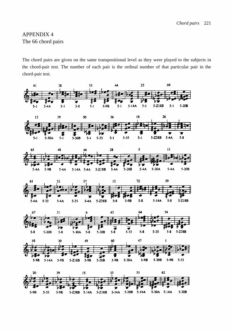
Chord pairs 221
APPENDIX 4 The 66 chord pairs
The chord pairs are given on the same transpositional level as they were played to the subjects in the chord-pair test. The number of each pair is the ordinal number of that particular pair in the chord-pair test.
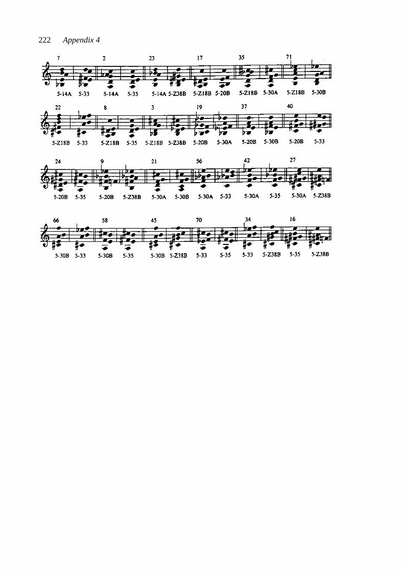
222 Appendix 4
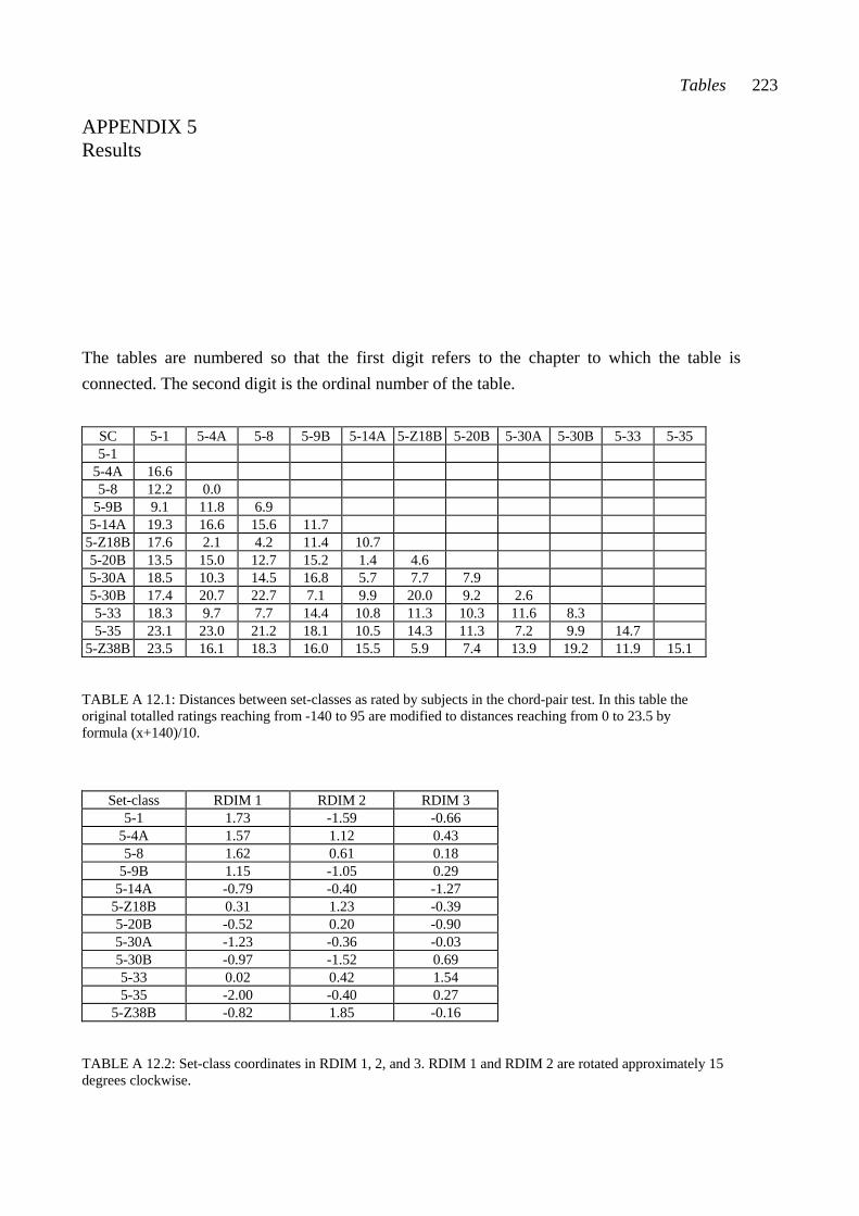
Tables 223
APPENDIX 5 Results
The tables are numbered so that the first digit refers to the chapter to which the table is connected. The second digit is the ordinal number of the table.
SC 5-1 5-4A 5-8 5-9B 5-14A 5-Z18B 5-20B 5-30A 5-30B 5-33 5-35 5-1
5-4A 16.6 5-8 12.2 0.0
5-9B 9.1 11.8 6.9 5-14A 19.3 16.6 15.6 11.7
5-Z18B 17.6 2.1 4.2 11.4 10.7 5-20B 13.5 15.0 12.7 15.2 1.4 4.6 5-30A 18.5 10.3 14.5 16.8 5.7 7.7 7.9 5-30B 17.4 20.7 22.7 7.1 9.9 20.0 9.2 2.6 5-33 18.3 9.7 7.7 14.4 10.8 11.3 10.3 11.6 8.3 5-35 23.1 23.0 21.2 18.1 10.5 14.3 11.3 7.2 9.9 14.7
5-Z38B 23.5 16.1 18.3 16.0 15.5 5.9 7.4 13.9 19.2 11.9 15.1 TABLE A 12.1: Distances between set-classes as rated by subjects in the chord-pair test. In this table the original totalled ratings reaching from -140 to 95 are modified to distances reaching from 0 to 23.5 by formula (x+140)/10.
Set-class RDIM 1 RDIM 2 RDIM 3
5-1 1.73 -1.59 -0.66 5-4A 1.57 1.12 0.43 5-8 1.62 0.61 0.18
5-9B 1.15 -1.05 0.29 5-14A -0.79 -0.40 -1.27
5-Z18B 0.31 1.23 -0.39 5-20B -0.52 0.20 -0.90 5-30A -1.23 -0.36 -0.03 5-30B -0.97 -1.52 0.69 5-33 0.02 0.42 1.54 5-35 -2.00 -0.40 0.27
5-Z38B -0.82 1.85 -0.16
TABLE A 12.2: Set-class coordinates in RDIM 1, 2, and 3. RDIM 1 and RDIM 2 are rotated approximately 15 degrees clockwise.
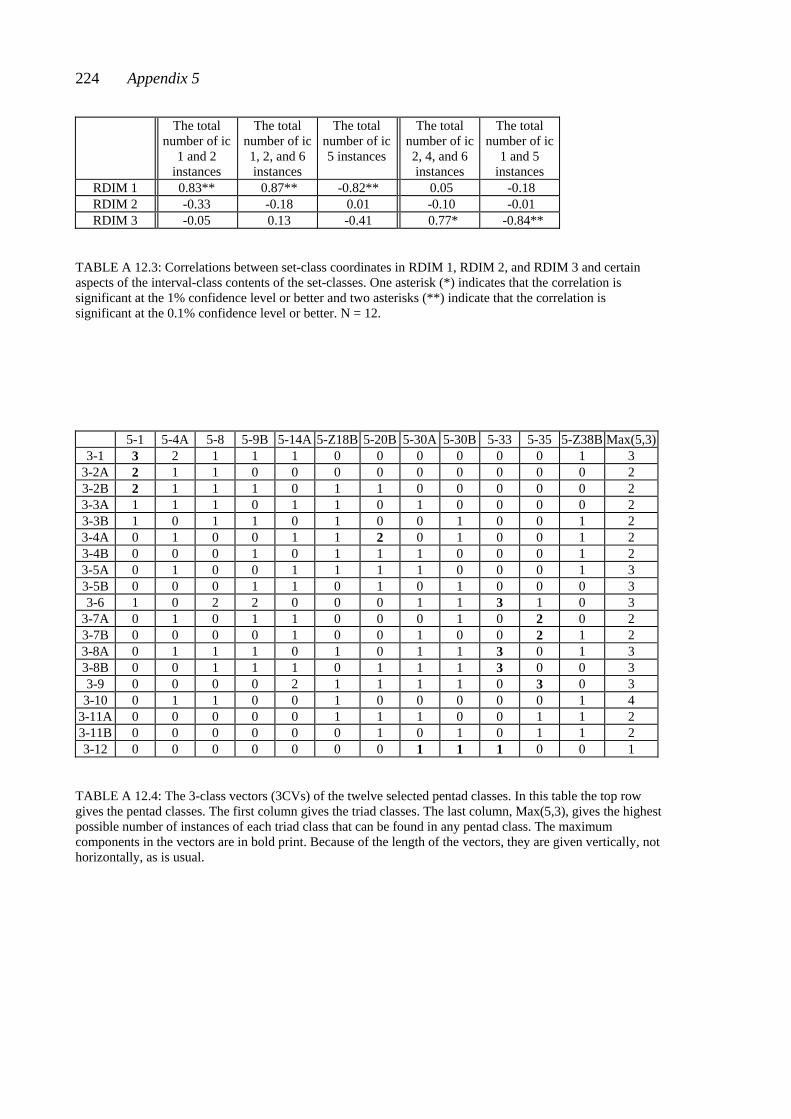
224 Appendix 5
The total
number of ic 1 and 2
instances
The total number of ic 1, 2, and 6 instances
The total number of ic 5 instances
The total number of ic 2, 4, and 6 instances
The total number of ic
1 and 5 instances
RDIM 1 0.83** 0.87** -0.82** 0.05 -0.18 RDIM 2 -0.33 -0.18 0.01 -0.10 -0.01 RDIM 3 -0.05 0.13 -0.41 0.77* -0.84**
TABLE A 12.3: Correlations between set-class coordinates in RDIM 1, RDIM 2, and RDIM 3 and certain aspects of the interval-class contents of the set-classes. One asterisk (*) indicates that the correlation is significant at the 1% confidence level or better and two asterisks (**) indicate that the correlation is significant at the 0.1% confidence level or better. N = 12.
5-1 5-4A 5-8 5-9B 5-14A 5-Z18B 5-20B 5-30A 5-30B 5-33 5-35 5-Z38B Max(5,3)3-1 3 2 1 1 1 0 0 0 0 0 0 1 3
3-2A 2 1 1 0 0 0 0 0 0 0 0 0 2 3-2B 2 1 1 1 0 1 1 0 0 0 0 0 2 3-3A 1 1 1 0 1 1 0 1 0 0 0 0 2 3-3B 1 0 1 1 0 1 0 0 1 0 0 1 2 3-4A 0 1 0 0 1 1 2 0 1 0 0 1 2 3-4B 0 0 0 1 0 1 1 1 0 0 0 1 2 3-5A 0 1 0 0 1 1 1 1 0 0 0 1 3 3-5B 0 0 0 1 1 0 1 0 1 0 0 0 3 3-6 1 0 2 2 0 0 0 1 1 3 1 0 3
3-7A 0 1 0 1 1 0 0 0 1 0 2 0 2 3-7B 0 0 0 0 1 0 0 1 0 0 2 1 2 3-8A 0 1 1 1 0 1 0 1 1 3 0 1 3 3-8B 0 0 1 1 1 0 1 1 1 3 0 0 3 3-9 0 0 0 0 2 1 1 1 1 0 3 0 3 3-10 0 1 1 0 0 1 0 0 0 0 0 1 4
3-11A 0 0 0 0 0 1 1 1 0 0 1 1 2 3-11B 0 0 0 0 0 0 1 0 1 0 1 1 2 3-12 0 0 0 0 0 0 0 1 1 1 0 0 1
TABLE A 12.4: The 3-class vectors (3CVs) of the twelve selected pentad classes. In this table the top row gives the pentad classes. The first column gives the triad classes. The last column, Max(5,3), gives the highest possible number of instances of each triad class that can be found in any pentad class. The maximum components in the vectors are in bold print. Because of the length of the vectors, they are given vertically, not horizontally, as is usual.
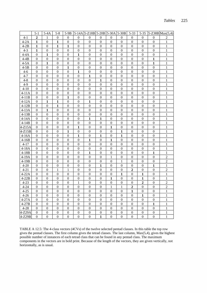
Tables 225
5-1 5-4A 5-8 5-9B 5-14A 5-Z18B 5-20B 5-30A 5-30B 5-33 5-35 5-Z38B Max(5,4)
4-1 2 1 0 0 0 0 0 0 0 0 0 0 2 4-2A 1 0 1 0 0 0 0 0 0 0 0 0 1 4-2B 1 0 1 1 0 0 0 0 0 0 0 0 1 4-3 1 0 0 0 0 0 0 0 0 0 0 0 1
4-4A 0 1 0 0 1 0 0 0 0 0 0 0 1 4-4B 0 0 0 0 0 0 0 0 0 0 0 1 1 4-5A 0 1 0 0 0 0 0 0 0 0 0 1 1 4-5B 0 0 0 1 0 0 0 0 0 0 0 0 1 4-6 0 0 0 0 1 0 0 0 0 0 0 0 1 4-7 0 0 0 0 0 1 0 0 0 0 0 0 1 4-8 0 0 0 0 0 0 1 0 0 0 0 0 1 4-9 0 0 0 0 0 0 0 0 0 0 0 0 1 4-10 0 0 0 0 0 0 0 0 0 0 0 0 1
4-11A 0 0 0 0 0 0 0 0 0 0 0 0 1 4-11B 0 0 0 1 0 0 0 0 0 0 0 0 1 4-12A 0 1 1 0 0 1 0 0 0 0 0 0 1 4-12B 0 0 1 0 0 0 0 0 0 0 0 0 1 4-13A 0 1 0 0 0 0 0 0 0 0 0 0 1 4-13B 0 0 0 0 0 0 0 0 0 0 0 0 1 4-14A 0 0 0 0 0 1 1 0 0 0 0 0 1 4-14B 0 0 0 0 0 0 0 0 0 0 0 0 1
4-Z15A 0 0 0 0 1 0 0 1 0 0 0 0 1 4-Z15B 0 0 0 1 0 0 0 0 1 0 0 0 1 4-16A 0 0 0 0 1 0 1 0 1 0 0 0 1 4-16B 0 0 0 0 0 1 0 1 0 0 0 0 1 4-17 0 0 0 0 0 0 0 0 0 0 0 0 1
4-18A 0 0 0 0 0 0 0 0 0 0 0 0 1 4-18B 0 0 0 0 0 1 0 0 0 0 0 1 1 4-19A 0 0 0 0 0 0 0 1 0 0 0 0 2 4-19B 0 0 0 0 0 0 0 0 1 0 0 0 2 4-20 0 0 0 0 0 0 1 0 0 0 0 1 1 4-21 0 0 1 1 0 0 0 0 0 2 0 0 2
4-22A 0 0 0 0 0 0 0 0 1 0 1 0 1 4-22B 0 0 0 0 0 0 0 1 0 0 1 0 1 4-23 0 0 0 0 1 0 0 0 0 0 2 0 2 4-24 0 0 0 0 0 0 0 1 1 2 0 0 2 4-25 0 0 0 0 0 0 0 0 0 1 0 0 1 4-26 0 0 0 0 0 0 0 0 0 0 1 0 1
4-27A 0 0 0 0 0 0 0 0 0 0 0 0 1 4-27B 0 0 0 0 0 0 0 0 0 0 0 1 1 4-28 0 0 0 0 0 0 0 0 0 0 0 0 1
4-Z29A 0 0 0 0 0 0 0 0 0 0 0 0 1 4-Z29B 0 0 0 0 0 0 1 0 0 0 0 0 1 TABLE A 12.5: The 4-class vectors (4CVs) of the twelve selected pentad classes. In this table the top row gives the pentad classes. The first column gives the tetrad classes. The last column, Max(5,4), gives the highest possible number of instances of each tetrad class that can be found in any pentad class. The maximum components in the vectors are in bold print. Because of the length of the vectors, they are given vertically, not horizontally, as is usual.
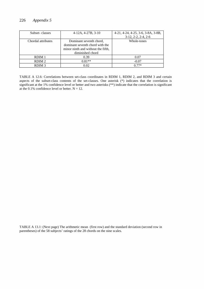
226 Appendix 5
Subset- classes 4-12A, 4-27B, 3-10 4-21, 4-24, 4-25, 3-6, 3-8A, 3-8B,
3-12, 2-2, 2-4, 2-6 Chordal attributes Dominant seventh chord,
dominant seventh chord with the minor ninth and without the fifth,
diminished chord
Whole-tones
RDIM 1 0.39 0.07 RDIM 2 0.81** -0.07 RDIM 3 0.02 0.77*
TABLE A 12.6: Correlations between set-class coordinates in RDIM 1, RDIM 2, and RDIM 3 and certain aspects of the subset-class contents of the set-classes. One asterisk (*) indicates that the correlation is significant at the 1% confidence level or better and two asterisks (**) indicate that the correlation is significant at the 0.1% confidence level or better. N = 12.
TABLE A 13.1: (Next page) The arithmetic mean (first row) and the standard deviation (second row in parentheses) of the 58 subjects’ ratings of the 28 chords on the nine scales.
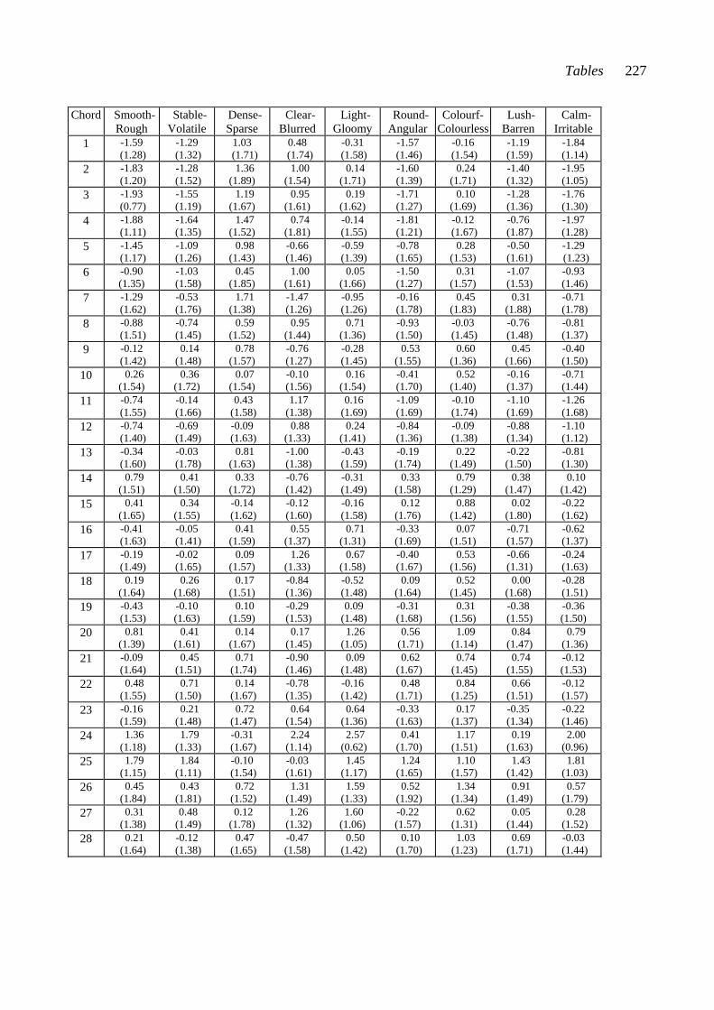
Tables 227
Chord Smooth-
Rough Stable- Volatile
Dense- Sparse
Clear- Blurred
Light- Gloomy
Round- Angular
Colourf- Colourless
Lush- Barren
Calm- Irritable
1 -1.59 (1.28)
-1.29 (1.32)
1.03 (1.71)
0.48 (1.74)
-0.31 (1.58)
-1.57 (1.46)
-0.16 (1.54)
-1.19 (1.59)
-1.84 (1.14)
2 -1.83 (1.20)
-1.28 (1.52)
1.36 (1.89)
1.00 (1.54)
0.14 (1.71)
-1.60 (1.39)
0.24 (1.71)
-1.40 (1.32)
-1.95 (1.05)
3 -1.93 (0.77)
-1.55 (1.19)
1.19 (1.67)
0.95 (1.61)
0.19 (1.62)
-1.71 (1.27)
0.10 (1.69)
-1.28 (1.36)
-1.76 (1.30)
4 -1.88 (1.11)
-1.64 (1.35)
1.47 (1.52)
0.74 (1.81)
-0.14 (1.55)
-1.81 (1.21)
-0.12 (1.67)
-0.76 (1.87)
-1.97 (1.28)
5 -1.45 (1.17)
-1.09 (1.26)
0.98 (1.43)
-0.66 (1.46)
-0.59 (1.39)
-0.78 (1.65)
0.28 (1.53)
-0.50 (1.61)
-1.29 (1.23)
6 -0.90 (1.35)
-1.03 (1.58)
0.45 (1.85)
1.00 (1.61)
0.05 (1.66)
-1.50 (1.27)
0.31 (1.57)
-1.07 (1.53)
-0.93 (1.46)
7 -1.29 (1.62)
-0.53 (1.76)
1.71 (1.38)
-1.47 (1.26)
-0.95 (1.26)
-0.16 (1.78)
0.45 (1.83)
0.31 (1.88)
-0.71 (1.78)
8 -0.88 (1.51)
-0.74 (1.45)
0.59 (1.52)
0.95 (1.44)
0.71 (1.36)
-0.93 (1.50)
-0.03 (1.45)
-0.76 (1.48)
-0.81 (1.37)
9 -0.12 (1.42)
0.14 (1.48)
0.78 (1.57)
-0.76 (1.27)
-0.28 (1.45)
0.53 (1.55)
0.60 (1.36)
0.45 (1.66)
-0.40 (1.50)
10 0.26 (1.54)
0.36 (1.72)
0.07 (1.54)
-0.10 (1.56)
0.16 (1.54)
-0.41 (1.70)
0.52 (1.40)
-0.16 (1.37)
-0.71 (1.44)
11 -0.74 (1.55)
-0.14 (1.66)
0.43 (1.58)
1.17 (1.38)
0.16 (1.69)
-1.09 (1.69)
-0.10 (1.74)
-1.10 (1.69)
-1.26 (1.68)
12 -0.74 (1.40)
-0.69 (1.49)
-0.09 (1.63)
0.88 (1.33)
0.24 (1.41)
-0.84 (1.36)
-0.09 (1.38)
-0.88 (1.34)
-1.10 (1.12)
13 -0.34 (1.60)
-0.03 (1.78)
0.81 (1.63)
-1.00 (1.38)
-0.43 (1.59)
-0.19 (1.74)
0.22 (1.49)
-0.22 (1.50)
-0.81 (1.30)
14 0.79 (1.51)
0.41 (1.50)
0.33 (1.72)
-0.76 (1.42)
-0.31 (1.49)
0.33 (1.58)
0.79 (1.29)
0.38 (1.47)
0.10 (1.42)
15 0.41 (1.65)
0.34 (1.55)
-0.14 (1.62)
-0.12 (1.60)
-0.16 (1.58)
0.12 (1.76)
0.88 (1.42)
0.02 (1.80)
-0.22 (1.62)
16 -0.41 (1.63)
-0.05 (1.41)
0.41 (1.59)
0.55 (1.37)
0.71 (1.31)
-0.33 (1.69)
0.07 (1.51)
-0.71 (1.57)
-0.62 (1.37)
17 -0.19 (1.49)
-0.02 (1.65)
0.09 (1.57)
1.26 (1.33)
0.67 (1.58)
-0.40 (1.67)
0.53 (1.56)
-0.66 (1.31)
-0.24 (1.63)
18 0.19 (1.64)
0.26 (1.68)
0.17 (1.51)
-0.84 (1.36)
-0.52 (1.48)
0.09 (1.64)
0.52 (1.45)
0.00 (1.68)
-0.28 (1.51)
19 -0.43 (1.53)
-0.10 (1.63)
0.10 (1.59)
-0.29 (1.53)
0.09 (1.48)
-0.31 (1.68)
0.31 (1.56)
-0.38 (1.55)
-0.36 (1.50)
20 0.81 (1.39)
0.41 (1.61)
0.14 (1.67)
0.17 (1.45)
1.26 (1.05)
0.56 (1.71)
1.09 (1.14)
0.84 (1.47)
0.79 (1.36)
21 -0.09 (1.64)
0.45 (1.51)
0.71 (1.74)
-0.90 (1.46)
0.09 (1.48)
0.62 (1.67)
0.74 (1.45)
0.74 (1.55)
-0.12 (1.53)
22 0.48 (1.55)
0.71 (1.50)
0.14 (1.67)
-0.78 (1.35)
-0.16 (1.42)
0.48 (1.71)
0.84 (1.25)
0.66 (1.51)
-0.12 (1.57)
23 -0.16 (1.59)
0.21 (1.48)
0.72 (1.47)
0.64 (1.54)
0.64 (1.36)
-0.33 (1.63)
0.17 (1.37)
-0.35 (1.34)
-0.22 (1.46)
24 1.36 (1.18)
1.79 (1.33)
-0.31 (1.67)
2.24 (1.14)
2.57 (0.62)
0.41 (1.70)
1.17 (1.51)
0.19 (1.63)
2.00 (0.96)
25 1.79 (1.15)
1.84 (1.11)
-0.10 (1.54)
-0.03 (1.61)
1.45 (1.17)
1.24 (1.65)
1.10 (1.57)
1.43 (1.42)
1.81 (1.03)
26 0.45 (1.84)
0.43 (1.81)
0.72 (1.52)
1.31 (1.49)
1.59 (1.33)
0.52 (1.92)
1.34 (1.34)
0.91 (1.49)
0.57 (1.79)
27 0.31 (1.38)
0.48 (1.49)
0.12 (1.78)
1.26 (1.32)
1.60 (1.06)
-0.22 (1.57)
0.62 (1.31)
0.05 (1.44)
0.28 (1.52)
28 0.21 (1.64)
-0.12 (1.38)
0.47 (1.65)
-0.47 (1.58)
0.50 (1.42)
0.10 (1.70)
1.03 (1.23)
0.69 (1.71)
-0.03 (1.44)
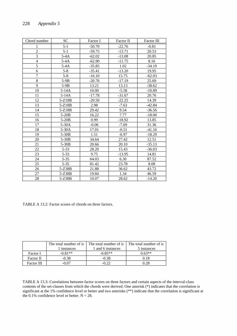
228 Appendix 5
Chord number SC Factor I Factor II Factor III
1 5-1 -50.70 -22.76 -0.81 2 5-1 -59.75 -13.71 20.53 3 5-4A -62.02 -13.08 20.85 4 5-4A -62.90 -11.75 8.16 5 5-4A -35.85 1.02 -34.19 6 5-8 -35.41 -13.20 19.95 7 5-8 -16.10 15.75 -62.03 8 5-9B -20.76 -17.19 25.69 9 5-9B 13.21 13.13 -38.62
10 5-14A 10.00 -5.58 -10.89 11 5-14A -17.78 -31.67 20.76 12 5-Z18B -20.50 -22.25 14.39 13 5-Z18B 2.98 -7.63 -42.84 14 5-Z18B 29.42 9.54 -36.56 15 5-20B 16.22 7.77 -18.00 16 5-20B 0.99 -18.92 13.85 17 5-30A -0.06 -7.69 31.36 18 5-30A 17.01 -0.51 -41.16 19 5-30B 1.51 -6.97 -18.29 20 5-30B 34.64 27.42 12.51 21 5-30B 20.66 20.10 -35.13 22 5-33 28.20 15.43 -36.03 23 5-33 9.75 -13.95 14.81 24 5-35 64.03 6.30 87.52 25 5-35 81.42 23.78 8.08 26 5-Z38B 21.88 36.62 43.72 27 5-Z38B 19.84 1.34 46.59 28 5-Z38B 10.07 28.62 -14.20
TABLE A 13.2: Factor scores of chords on three factors.
The total number of ic
1 instances The total number of ic
1 and 6 instances The total number of ic
5 instances Factor I -0.81** -0.85** 0.63** Factor II -0.38 -0.38 0.18 Factor III -0.07 -0.22 0.28
TABLE A 13.3: Correlations between factor scores on three factors and certain aspects of the interval-class contents of the set-classes from which the chords were derived. One asterisk (*) indicates that the correlation is significant at the 1% confidence level or better and two asterisks (**) indicate that the correlation is significant at the 0.1% confidence level or better. N = 28.
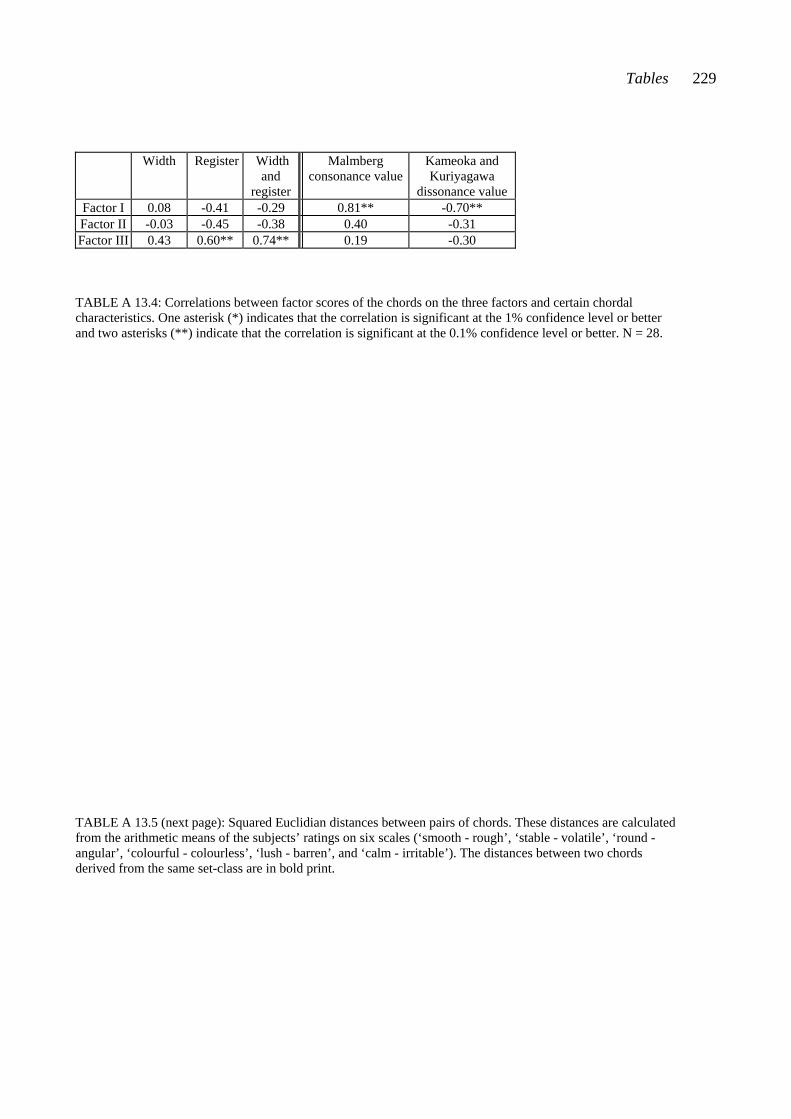
Tables 229
Width Register Width
and register
Malmberg consonance value
Kameoka and Kuriyagawa
dissonance value Factor I 0.08 -0.41 -0.29 0.81** -0.70** Factor II -0.03 -0.45 -0.38 0.40 -0.31 Factor III 0.43 0.60** 0.74** 0.19 -0.30
TABLE A 13.4: Correlations between factor scores of the chords on the three factors and certain chordal characteristics. One asterisk (*) indicates that the correlation is significant at the 1% confidence level or better and two asterisks (**) indicate that the correlation is significant at the 0.1% confidence level or better. N = 28.
TABLE A 13.5 (next page): Squared Euclidian distances between pairs of chords. These distances are calculated from the arithmetic means of the subjects’ ratings on six scales (‘smooth - rough’, ‘stable - volatile’, ‘round - angular’, ‘colourful - colourless’, ‘lush - barren’, and ‘calm - irritable’). The distances between two chords derived from the same set-class are in bold print.
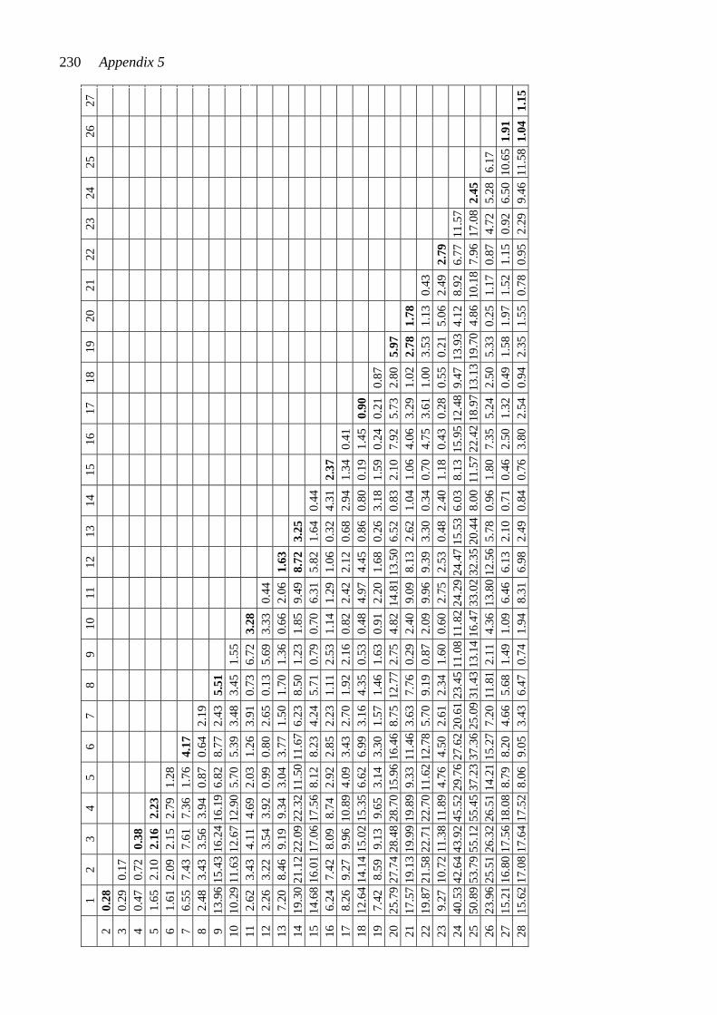
1 2
3 4
5 6
7 8
9 10
11
12
13
14
15
16
17
18
19
20
21
22
23
24
25
26
27
2
0.28
3
0.29
0.
17
4 0.
47
0.72
0.38
5 1.
65
2.10
2.16
2.23
6 1.
61
2.09
2.15
2.79
1.
28
7 6.
55
7.43
7.61
7.36
1.
76
4.17
8 2.
48
3.43
3.56
3.94
0.
87
0.64
2.
19
9
13.9
6 15
.43
16.2
416
.19
6.82
8.
77
2.43
5.51
10
10
.29
11.6
312
.67
12.9
0 5.
70
5.39
3.
483.
451.
55
11
2.
62
3.43
4.11
4.69
2.
03
1.26
3.
910.
736.
723.
28
12
2.26
3.
223.
543.
92
0.99
0.
80
2.65
0.13
5.69
3.33
0.44
13
7.20
8.
469.
199.
34
3.04
3.
77
1.50
1.70
1.36
0.66
2.06
1.63
14
19
.30
21.1
222
.09
22.3
2 11
.50
11.6
7 6.
238.
501.
231.
859.
498.
723.
25
15
14
.68
16.0
117
.06
17.5
6 8.
12
8.23
4.
245.
710.
790.
706.
315.
821.
640.
44
16
6.24
7.
428.
098.
74
2.92
2.
85
2.23
1.11
2.53
1.14
1.29
1.06
0.32
4.31
2.37
17
8.26
9.
279.
9610
.89
4.09
3.
43
2.70
1.92
2.16
0.82
2.42
2.12
0.68
2.94
1.34
0.41
18
12.6
4 14
.14
15.0
215
.35
6.62
6.
99
3.16
4.35
0.53
0.48
4.97
4.45
0.86
0.80
0.19
1.45
0.
90
19
7.
42
8.59
9.13
9.65
3.
14
3.30
1.
571.
461.
630.
912.
201.
680.
263.
181.
590.
24
0.21
0.87
20
25
.79
27.7
428
.48
28.7
0 15
.96
16.4
6 8.
7512
.77
2.75
4.82
14.8
113
.50
6.52
0.83
2.10
7.92
5.
732.
805.
97
21
17
.57
19.1
319
.99
19.8
9 9.
33 1
1.46
3.6
37.
760.
292.
409.
098.
132.
621.
041.
064.
06
3.29
1.02
2.78
1.78
22
19
.87
21.5
822
.71
22.7
0 11
.62
12.7
8 5.
709.
190.
872.
099.
969.
393.
300.
340.
704.
75
3.61
1.00
3.53
1.13
0.43
23
9.27
10.
7211
.38
11.8
9 4.
76
4.50
2.
612.
341.
600.
602.
752.
530.
482.
401.
180.
43
0.28
0.55
0.21
5.06
2.49
2.79
24
40
.53
42.6
443
.92
45.5
2 29
.76
27.6
2 20
.61
23.4
511
.08
11.8
224
.29
24.4
715
.53
6.03
8.13
15.9
5 12
.48
9.47
13.9
34.
128.
926.
7711
.57
25
50.8
9 53
.79
55.1
255
.45
37.2
3 37
.36
25.0
931
.43
13.1
416
.47
33.0
232
.35
20.4
48.
0011
.57
22.4
2 18
.97
13.1
319
.70
4.86
10.1
87.
9617
.08
2.45
26
23
.96
25.5
126
.32
26.5
1 14
.21
15.2
7 7.
2011
.81
2.11
4.36
13.8
012
.56
5.78
0.96
1.80
7.35
5.
242.
505.
330.
251.
170.
874.
725.
286.
17
27
15
.21
16.8
017
.56
18.0
8 8.
79
8.20
4.
665.
681.
491.
096.
466.
132.
100.
710.
462.
50
1.32
0.49
1.58
1.97
1.52
1.15
0.92
6.50
10.6
51.
91
28
15
.62
17.0
817
.64
17.5
2 8.
06
9.05
3.
436.
470.
741.
948.
316.
982.
490.
840.
763.
80
2.54
0.94
2.35
1.55
0.78
0.95
2.29
9.46
11.5
81.
04
1.15
230 Appendix 5
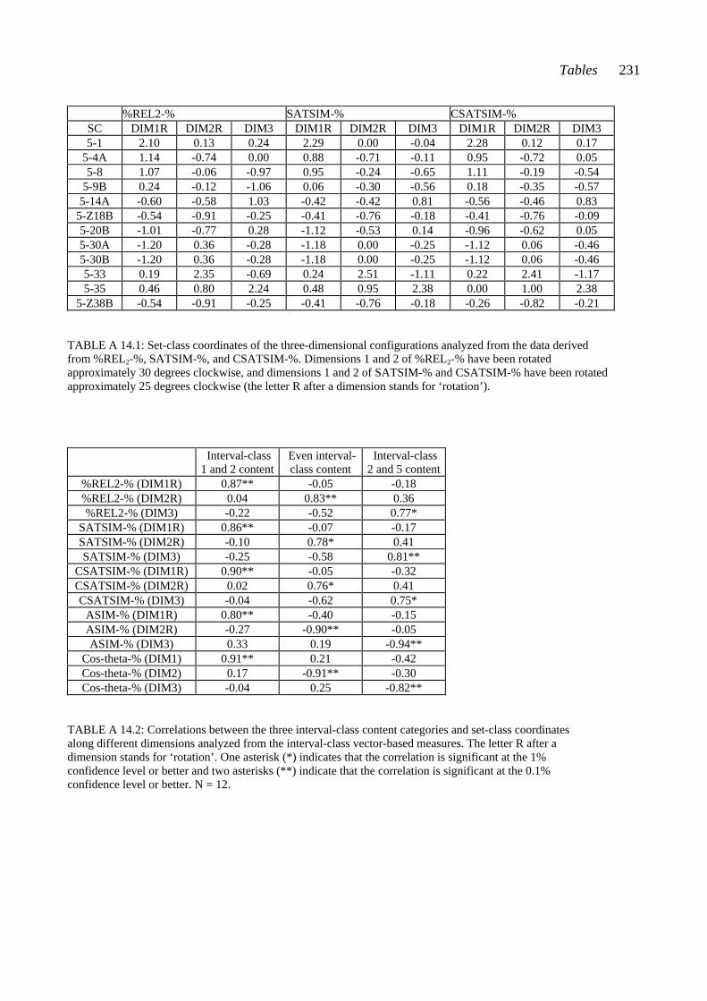
Tables 231
%REL2-% SATSIM-% CSATSIM-%
SC DIM1R DIM2R DIM3 DIM1R DIM2R DIM3 DIM1R DIM2R DIM3 5-1 2.10 0.13 0.24 2.29 0.00 -0.04 2.28 0.12 0.17
5-4A 1.14 -0.74 0.00 0.88 -0.71 -0.11 0.95 -0.72 0.05 5-8 1.07 -0.06 -0.97 0.95 -0.24 -0.65 1.11 -0.19 -0.54
5-9B 0.24 -0.12 -1.06 0.06 -0.30 -0.56 0.18 -0.35 -0.57 5-14A -0.60 -0.58 1.03 -0.42 -0.42 0.81 -0.56 -0.46 0.83
5-Z18B -0.54 -0.91 -0.25 -0.41 -0.76 -0.18 -0.41 -0.76 -0.09 5-20B -1.01 -0.77 0.28 -1.12 -0.53 0.14 -0.96 -0.62 0.05 5-30A -1.20 0.36 -0.28 -1.18 0.00 -0.25 -1.12 0.06 -0.46 5-30B -1.20 0.36 -0.28 -1.18 0.00 -0.25 -1.12 0.06 -0.46 5-33 0.19 2.35 -0.69 0.24 2.51 -1.11 0.22 2.41 -1.17 5-35 0.46 0.80 2.24 0.48 0.95 2.38 0.00 1.00 2.38
5-Z38B -0.54 -0.91 -0.25 -0.41 -0.76 -0.18 -0.26 -0.82 -0.21 TABLE A 14.1: Set-class coordinates of the three-dimensional configurations analyzed from the data derived from %REL2-%, SATSIM-%, and CSATSIM-%. Dimensions 1 and 2 of %REL2-% have been rotated approximately 30 degrees clockwise, and dimensions 1 and 2 of SATSIM-% and CSATSIM-% have been rotated approximately 25 degrees clockwise (the letter R after a dimension stands for ‘rotation’). Interval-class
1 and 2 content Even interval- class content
Interval-class 2 and 5 content
%REL2-% (DIM1R) 0.87** -0.05 -0.18 %REL2-% (DIM2R) 0.04 0.83** 0.36 %REL2-% (DIM3) -0.22 -0.52 0.77*
SATSIM-% (DIM1R) 0.86** -0.07 -0.17 SATSIM-% (DIM2R) -0.10 0.78* 0.41 SATSIM-% (DIM3) -0.25 -0.58 0.81**
CSATSIM-% (DIM1R) 0.90** -0.05 -0.32 CSATSIM-% (DIM2R) 0.02 0.76* 0.41 CSATSIM-% (DIM3) -0.04 -0.62 0.75*
ASIM-% (DIM1R) 0.80** -0.40 -0.15 ASIM-% (DIM2R) -0.27 -0.90** -0.05 ASIM-% (DIM3) 0.33 0.19 -0.94**
Cos-theta-% (DIM1) 0.91** 0.21 -0.42 Cos-theta-% (DIM2) 0.17 -0.91** -0.30 Cos-theta-% (DIM3) -0.04 0.25 -0.82**
TABLE A 14.2: Correlations between the three interval-class content categories and set-class coordinates along different dimensions analyzed from the interval-class vector-based measures. The letter R after a dimension stands for ‘rotation’. One asterisk (*) indicates that the correlation is significant at the 1% confidence level or better and two asterisks (**) indicate that the correlation is significant at the 0.1% confidence level or better. N = 12.

232 Appendix 5
ASIM-% Cos-theta-%
SC DIM1R DIM2R DIM3 DIM1 DIM2 DIM3 5-1 2.42 -0.46 0.15 2.06 0.72 -0.29
5-4A 1.15 0.56 0.52 1.12 1.19 0.06 5-8 0.82 -0.56 0.71 1.72 -0.03 0.21
5-9B 0.00 -0.28 0.59 0.96 -0.48 0.47 5-14A -0.24 1.01 -0.55 -0.96 0.72 -0.94
5-Z18B -0.22 0.99 0.46 -0.79 0.87 0.63 5-20B -0.93 1.12 -0.01 -1.39 0.66 0.14 5-30A -1.30 -0.09 -0.05 -0.87 -0.86 0.64 5-30B -1.30 -0.09 -0.05 -0.87 -0.86 0.64 5-33 -0.87 -3.15 0.10 0.52 -2.44 0.06 5-35 0.69 -0.06 -2.34 -0.71 -0.37 -2.27
5-Z38B -0.22 0.99 0.46 -0.79 0.87 0.63 TABLE A 14.3: Set-class coordinates of the three-dimensional configurations analyzed from the data derived from ASIM-% and Cosθ-%. Dimensions 1 and 2 of ASIM-% have been rotated 90 degrees clockwise (the letter R after a dimension stands for ‘rotation’).
ATMEMB-% REL-% RECREL-%
SC DIM1 DIM2 DIM3 DIM1 DIM2 DIM3 DIM1 DIM2 DIM3 5-1 2.01 0.93 -0.88 1.98 0.52 -1.00 2.22 0.26 -0.57
5-4A 0.87 1.27 -0.20 0.91 1.32 -0.34 1.09 1.11 -0.13 5-8 1.70 -0.32 0.08 1.66 -0.25 0.19 1.54 0.15 0.51
5-9B 0.80 -0.80 0.02 1.02 -0.62 0.31 0.64 -0.24 0.67 5-14A -1.02 0.59 -0.90 -1.14 0.45 -0.90 -0.89 0.45 -0.89
5-Z18B -0.17 1.01 0.93 -0.26 1.13 0.87 -0.48 1.07 0.44 5-20B -1.23 0.71 0.82 -1.30 0.76 0.71 -1.39 0.58 0.01 5-30A -0.75 -0.79 0.25 -0.94 -0.74 0.35 -1.24 -0.41 0.43 5-30B -0.64 -1.00 -0.16 -0.76 -1.03 0.14 -1.12 -0.73 0.47 5-33 0.70 -2.34 0.45 0.61 -2.10 0.73 0.50 -2.44 0.95 5-35 -1.88 -0.33 -1.43 -1.23 -0.69 -1.87 -0.35 -0.97 -2.27
5-Z38B -0.39 1.06 1.02 -0.55 1.25 0.82 -0.53 1.17 0.37 TABLE A 14.4: Set-class coordinates of the three-dimensional configurations analyzed from the data derived from ATMEMB-%, REL-%, and RECREL-%.
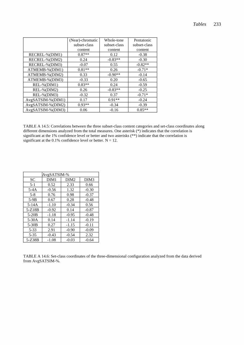
Tables 233
(Near)-chromatic
subset-class content
Whole-tone subset-class
content
Pentatonic subset-class
content RECREL-%(DIM1) 0.87** 0.12 -0.38 RECREL-%(DIM2) 0.24 -0.83** -0.30 RECREL-%(DIM3) -0.07 0.55 -0.82**
ATMEMB-%(DIM1) 0.81** 0.26 -0.71* ATMEMB-%(DIM2) 0.33 -0.90** -0.14 ATMEMB-%(DIM3) -0.33 0.20 -0.65
REL-%(DIM1) 0.83** 0.24 -0.59 REL-%(DIM2) 0.26 -0.83** -0.25 REL-%(DIM3) -0.32 0.37 -0.71*
AvgSATSIM-%(DIM1) 0.17 0.91** -0.24 AvgSATSIM-%(DIM2) 0.93** -0.34 -0.39 AvgSATSIM-%(DIM3) 0.06 -0.16 0.85**
TABLE A 14.5: Correlations between the three subset-class content categories and set-class coordinates along different dimensions analyzed from the total measures. One asterisk (*) indicates that the correlation is significant at the 1% confidence level or better and two asterisks (**) indicate that the correlation is significant at the 0.1% confidence level or better. N = 12. AvgSATSIM-%
SC DIM1 DIM2 DIM3 5-1 0.52 2.33 0.66
5-4A -0.56 1.32 -0.30 5-8 0.76 0.98 -0.37
5-9B 0.67 0.28 -0.48 5-14A -1.10 -0.34 0.56
5-Z18B -0.92 0.14 -0.87 5-20B -1.18 -0.95 -0.48 5-30A 0.14 -1.14 -0.19 5-30B 0.27 -1.15 -0.11 5-33 2.91 -0.90 -0.09 5-35 -0.43 -0.54 2.32
5-Z38B -1.08 -0.03 -0.64
TABLE A 14.6: Set-class coordinates of the three-dimensional configuration analyzed from the data derived from AvgSATSIM-%.
BIBLIOGRAPHY OF CITED WORKS Abbreviations of journal names: CMR Contemporary Music Review JMT Journal of Music Theory JASA Journal of the Acoustical Society of America MP Music Perception MTO Music Theory Online PM Psychology of Music PNM Perspectives of New Music Alphonce, B. (1974): The Invariance Matrix. Ph. D. dissertation, Yale University. Arabie, P., Carrol, D. J., and DeSarbo, W. (1987): Three-Way Scaling and Clustering. Sage
University Paper series on Quantitative Applications in the Social Sciences, 07-065. Beverly Hills and London: Sage Publications.
Bachem, A. (1954): Time Factors in Relative and Absolute Pitch Determination. JASA, 26, 751-753.
Baird, J.W. (1917): Memory for Absolute Pitch; Studies in Psychology. In Titchener Commemorative Volume. Worcester.
Balkwill, L-L., Diamond, C.P., and Thompson, W.F. (1998): The Adjudication of Six Performances of a Chopin Etude: A Study of Expert Knowledge. PM, 26, 154-174.
Bigand, E. and Tillman, B. (1996): Does Formal Musical Structure Affect Perception of Musical Expressiveness? PM, 24, 3-17.
Bharucha, J.J. (1991): Pitch, Harmony and Neural Nets: A Psychological Perspective. In Todd, P.M. and Loy, D.G. (eds.): Music and Connectionism, 84-99. Massachusetts: The MIT Press.
Blowers, G.H. and Bacon-Shone, J. (1994): On Detecting the Differences in Jazz: A Reassessment of Comparative Methods of Measuring Perceptual Verticality. Empirical Studies of the Arts, 12, 41-58.

Bibliography 235
Bruner, C. L. (1984): The Perception of Contemporary Pitch Structures. MP, 2, 25-39. Buchler, M. (1998): Relative Saturation of Subsets and Interval Cycles as a Means for Determining
Set-Class Similarity. Ph. D. dissertation, University of Rochester. Burns, E. M. and Ward, W. D. (1982): Intervals, Scales and Tuning. In Deutsch, D. (ed.): The
Psychology of Music, 241-269. Series in Cognition and Perception. New York: Academic Press.
Butler, D. (1992): The Musician’s Guide to Perception and Cognition. New York: Schirmer. Carroll, D. J. and Wish, M. (1974a): Multidimensional Perceptual Models and Measurement
Methods. In Carterette, E. C. and Friedman, M. P. (eds.): Handbook of Perception, vol II. Psychophysical Judgment and Measurement, 391-447. Department of Psychology, University of California. New York: Academic Press.
Carroll, D. J. and Wish, M. (1974b): Models and Methods for Three-Way Multidimensional Scaling. In Krantz D. H., Atkinson, R. C., Luce, R. D., and Suppes, P. (eds.): Contemporary Developments in Mathematical Psychology, vol 2, 57-105. San Francisco: Freeman.
Castrén, M. (1989): Joukkoteorian peruskysymyksiä. Helsinki: Sibelius Academy. Castrén, M. (1994a): RECREL, A similarity measure for set-classes. Helsinki: Sibelius Academy. Castrén, M. (1994b): Unpublished computer programs for calculating similarity values. Castrén, M. (2000): Pairs of Chords as Objects Illuminating Set-Class Similarity: Some Viewpoints
and a Computer-Assisted Procedure to Create Test Materials for Listener Experiments. Electronic Journal of Music Theory and Analysis, 1, No 1.
Castrén, M. and Laurson, M. (2000): MacSet 3.1. A Pitch-Class Set-Theoretical Computer Program. Helsinki: Sibelius Academy. Downloading address: ftp://ftp.siba.fi/pub/mac/MacSet.sea.hqx.
Charbonneau, G., Hourdin, C., and Moussa, T. (1997): A Multidimensional Scaling Analysis of Musical Instruments’ Time Varying Spectra. Computer Music Journal, 21, 41-55.
Cook, N. D. (2000): Explaining Harmony: The Independence of Interval Dissonance and Chordal Tension. Paper presented at the XXVII International Congress of Psychology, Stockholm, Sweden.
Cronbach, L. J. (1990): Essentials of Psychological Testing. 5th Edition. New York: Harper and Row.
Cross, I. (1985): Music and Change: On the Establishment of Rules. In Howell, P., Cross, I., and West, R. (eds.): Musical Structure and Cognition, 1-20. Orlando, Florida: Academic Press.
Danner, G. (1985): The Use of Acoustic Measures of Dissonance to Characterize Pitch-Class Sets. MP, 3, 103-122.
236 Bibliography
Demske, T. R. (1995): Relating Sets: On Considering a Computational Model of Similarity Analysis. MTO, 1 No 2.
Deutsch, D. (1973): Octave Generalization of Specific Interference Effects in Memory for Tonal Pitch. Perception and Psychophysics, 13, 271-275.
Deutsch, D. (1982): The Procession of Pitch Combinations. In Deutsch D. (ed.): The Psychology of Music, 271-316. Series in Cognition and Perception. New York: Academic Press.
Deutsch, D. and Roll P.L. (1974): Error Patterns in Delayed Pitch Comparison as a Function of Relational Context. Journal of Experimental Psychology, 103, 1027-1034.
Dowling, W. J. and Harwood, D. L. (1986): Music Cognition. Series in Cognition and Perception. New York: Academic Press.
Eastlund, J.O. (1992): A Multidimensional Scaling Analysis of Musical Style. Journal of Research in Music Education, 204-215.
Ekholm, E. and Wapnick, J. (1997): Expert Consensus in Solo Voice Performance Evaluation. Journal of Voice - Official Journal of the Voice Foundation, 429-436.
Ericksson, T. (1986): The IC Max Point Structure, MM Vectors and Regions. JMT, 30, 95-111. Forte, A. (1963): Context and Continuity in an Atonal Work. A Set-Theoretic Approach. PNM, 1,
72-82. Forte, A. (1964): A Theory of Set-complexes for Music. JMT, 8, 136-183. Forte, A. (1973): The Structure of Atonal Music. New Haven and London: Yale University Press. Forte, A. (1985): Pitch-Class Set Analysis Today. Music Analysis, 4, 29-58. Friedmann, M. L. (1990): Ear Training for Twentieth-Century Music. New Haven and London:
Yale University Press. Garner, W.R. (1973): The Processing of Information and Structure. Hillsdale, New Jersey:
Erlbaum. Gibson, D. B. (1986): The Aural Perception of Nontraditional Chords in Selected Theoretical
Relationships: A Computer-Generated Experiment. Journal of Research in Music Education, 34, 5-23.
Gibson, D. B. (1988): The Aural Perception of Similarity in Nontraditional Chords Related by Octave Equivalence. Journal of Research in Music Education, 36, 5-17.
Gibson, D. B. (1993): The Effects of Pitch and Pitch-Class Content on the Aural Perception of Dissimilarity in Complementary Hexachords. Psychomusicology, 12, 58-72.
Goldstone, R. L. (1994): The Role of Similarity in Categorization: Providing a Groundwork. Cognition, 52, 125-157.
Goodman, N. (1972): Seven Strictures on Similarity. In Goodman, N. (ed.): Problems and Projects. New York: Bobbs-Merrill.
Bibliography 237
Grey, J.M. (1977): Multidimensional Perceptual Scaling of Musical Timbres. JASA, 61, 1270-1277. Hantz, E. (1984): Studies in Music Cognition: Comments from a Music Theorist. MP, 2, 245-264. Harris, S. (1989): A Proposed Classification of Chords in Early Twentieth-Century Music. New
York: Garland. Helmholtz, H. von (1863): Die Lehre von der Tonempfindungen als physiologische Grundlage für
die Theorie der Musik. Braunschweig: Verlag F. Vieweg & Sohn. Hermann, R. (1994): A General Measurement for Similarity Relations: A Heuristic for Constructing
or Evaluating Aspects of Possible Musical Grammars. Ph. D. dissertation, University of Rochester.
Hermann, R. (1995): Towards a New Analytical Method for Post-Tonal Music: A Response to Thomas Demske. MTO, 1 No 3.
Hindemith, P. (1937/1942): The Craft of Musical Composition, vol. 1: Theoretical Part (Trans. A. Mendel). New York: Associated Music.
Hoover, M. (1984): Set Constellations. PNM, 23, 164-179. Huron, D. (1994): Interval-Class Content in Equally Tempered Pitch-Class Sets: Common Scales
Exhibit Optimum Tonal Consonance. MP, 11, 289-305. Huron, D. (1989): Voice Denumerability in Polyphonic Music of Homogeneous Timbres. MP, 6,
361-382. Hutchinson, W. and Knopoff, L. (1978): The Acoustic Component of Western Consonance.
Interface, 7, 1-29. Hutchinson, W. and Knopoff, L. (1979): The Significance of the Acoustic Component of
Consonance in Western Triads. Journal of Musicological Research, 3, 5-22. Isaacson, E. (1990): Similarity of Interval-Class Content Between Pitch-Class Sets: The IcVSIM
Relation. JMT, 34, 1-28. Isaacson, E. (1992): Similarity of Interval-Class Content Between Pitch-Class Sets: The IcVSIM
Relation and Its Application. Ph. D. dissertation, Indiana University. Isaacson, E. (1996): Issues in the Study of Similarity in Atonal Music. MTO, 2 No 7. Isaacson, E. (1997): Neural Network Models for the Study of Post-Tonal Music. In Leman, M.
(ed.): Music, Gestalt, and Computing: Studies in Cognitive and Systematic Musicology, 237-250. Berlin: Springer-Verlag.
Iverson, P. and Krumhansl, C. L. (1993): Isolating the Dynamic Attributes of Musical Timbre. JASA, 94, 2595-2603.
Kameoka, A. and Kuriyagawa, M. (1969): Consonance Theory Part II: Consonance of Complex Tones and Its Calculation Method. JASA, 45, 1460-1469.
Karma, K. (1986): Musiikkipsykologian perusteet. Musiikkitieteen kirjasto 3, Suomen musiikkitieteellinen seura. Helsinki: Offset Oy.

238 Bibliography
Karma, K. and Komulainen, E. (1984): Käyttäytymistieteiden tilastomenetelmien jatkokurssi. Oy Gaudeamus Ab. Mänttä: Mäntän kirjapaino Oy.
Kendall, R.A. and Carterette, E.C. (1991): Perceptual Scaling of Simultaneous Wind Instrument Timbres. MP, 8, 369-404.
Krumhansl, C. L. and Kessler, E. (1982): Tracing the Dynamic Changes in Perceived Tonal Organization in a Spatial Representation of Musical Keys. Psychological Review, 89, 334-368.
Krumhansl, C. L., Sandell, G. J., and Sergeant, D. C. (1987): The Perception of Tone Hierarchies and Mirror Forms in Twelve-Tone Serial Music. MP, 5, 31-78.
Krumhansl, C. L. (1990): Cognitive Foundations of Musical Pitch. New York: Oxford University Press.
Kruskal, J. B. and Wish, M. (1978): Multidimensional Scaling. Sage University Paper Series on Quantitative Applications in the Social Sciences, 07-011. Beverly Hills and London: Sage Publications.
Lane, R.C. (1997): A Multidimensional Scaling Study of Seven Theoretical Indexes of Intervallic Similarity and Musicians’ Perceptions Among Twenty-One Pitch-Class Sets. Ph. D. Dissertation, University of North Carolina.
Lehtinen, T. and Niskanen, V. A. (1994): Tilastotieteen perusteet. Helsingin yliopisto, Lahden tutkimus- ja koulutuskeskus. Helsinki: Yliopistopaino.
Leman, M (1991): The Ontogenesis of Tonal Semantics: Results of a Computer Study. In Todd, P.M. and Loy, D.G. (eds): Music and Connectionism, 100-127. Massachusetts: The MIT Press.
Lerdahl, F. (1989): Atonal Prolognational Structure. CMR, 4, 65-87. Lewin, D. (1979/80): A Response to a Response: On PCSet Relatedness. PNM, 18, 498-502. Lord, C. H. (1981): Intervallic Similarity Relations in Atonal Set Theory. JMT, 25, 91-111. Lundin, R. W. (1967): An Objective Psychology of Music 2. ed. New York: The Ronald Press
Company. Malmberg, C.F. (1918): The Perception of Consonance and Dissonance. Psychological
Monographs 25, 93-133. Marvin, E. W. and Laprade, P. A. (1987): Relating Musical Contours: Extensions of a Theory for
Contour. JMT, 31, 225-267. Millar, J. (1984): The Aural Perception of Pitch-Class Set Relations: A Computer-Assisted
Investigation. Ph. D. dissertation, North Texas State University. Morris R. (1979/80): A Similarity Index for Pitch-Class Sets. PNM, 18, 445-460. Morris, R. (1982): Set Groups, Complementation, and Mappings among Pitch-Class Sets. JMT, 26,
101-144. Morris, R. (1987): Composition with Pitch-classes. New Haven and London: Yale University Press.
Bibliography 239
Nichols, J.P. (1991): A Factor-Analysis Approach to the Development of a Rating Scale for Snare Drum Performance. Dialogue in Instrumental Music Education, 11-31.
Nordenstreng, K. (1968): A Comparison between the Semantic Differential and Similarity Analysis in the Measurement of Musical Experience. Scandinavian Journal of Psychology, 9, 89-96.
Nosofsky, R. M. (1992): Exemplar-Based Approach to Relating Categorization, Identification, and Recognition. In Ashby, F. G. (ed.): Multidimensional Models of Perception and Cognition, 363-393. Hillsdale, New Jersey: Erlbaum.
Osgood, C. E., Suci, G. J., and Tannenbaum, P. H. (1957): The Measurement of Meaning. University of Illinois Press.
Plomp, P. (1976): Aspects of Tone Sensation. New York: Academic Press. Plomp, R. and Levelt, W.J.M. (1965): Tonal Consonance and Critical Bandwidth. JASA, 38, 548-
560. Plomp, R., Wagenaar, W.A., and Mimpen, A.M. (1973): Musical Interval Recognition with
Simultaneous Tones. Acustica, 29, 101-109. Prince, W. F. (1972): A Paradigm for Research on Music Listening. Journal of Research in Music
Education, 20, 445-455. Quinn, I. (1997): On Similarity, Relations, and Similarity Relations. Paper presented at the Society
for Music Theory Conference, Phoenix, Arizona. Rahn, J. (1979/80): Relating Sets. PNM, 18, 483-497. Rahn, J. (1980): Basic Atonal Theory. New York: Schirmer. Rahn, J. (1981/1989): Toward a Theory of Chord Progression. In Theory Only, 11 No. 1-2, 1-10. Rasch, R.A. and Plomp, R. (1982): The Perception of Musical Tones. In Deutsch, D. (ed.): The
Psychology of Music, 1-24. Series in Cognition and Perception. New York: Academic Press. Risset, J-C. and Wessel, D.L. (1982): Exploration of Timbre by Analysis and Synthesis. In Deutsch,
D.(ed.): The Psychology of Music, 25-58. Series in Cognition and Perception. New York: Academic Press.
Rogers, D. W. (1992): Interval-Class Content and Similarity Functions: A Critique of a Critique. A seminar handout. Eastman School of Music.
Rogers, D. W. (1999): A Geometric Approach to Pcset Similarity. PNM 37, 78-90. Samplaski, A.G. (2000): A Comparison of Perceived Chord Similarity and Predictions of Selected
Twentieth-Century Chord-Classification Schemes, Using Multidimensional Scaling and Cluster Analysis. Ph. D. dissertation, Indiana University.
Scott, D. and Isaacson E. J. (1998): The Interval Angle: A Similarity Measure for Pitch-Class Sets. PNM 36, 107-142.

240 Bibliography
Sethares, W.A. (1998): Tuning, Timbre, Spectrum, Scale. London: Springer-Verlag. Shepard, R. N. (1962): The Analysis of Proximities: Multidimensional Scaling with an Unknown
Distance Function. I. Psychometrika, 27, 125-140. Shepard, R. N. (1982): Structural Representations of Musical Pitch. In Deutsch, D. (ed.): The
Psychology of Music, 344-390. Series in Cognition and Perception. New York: Academic Press.
Soininvaara, O. (1983): Faktorianalyysista. In Vartia, Y.O. (ed.): Tilastotieteen sovellutuksista, 64-73. Helsingin yliopiston Tilastotieteen laitoksen opetusmonisteita, 3, 2nd ed.
Solomon, L. N. (1954): A Factorial Study of Complex Auditory Stimuli (Passive Sonar Sounds). Ph. D. dissertation, University of Illinois.
Stammers, D. (1994): Set Theory in the Perception of Atonal Pitch Relations. Ph. D. dissertation, Cambridge University.
Straus, J. N. (1990): Introduction to Post-Tonal Theory. New Jersey: Prentice Hall. Teitelbaum, R. (1965): Intervallic Relations in Atonal Music. JMT, 9, 72-127. Tenney, J. (1988): A History of ’Consonance’ and ’Dissonance’. New York: Excelsior Music
Publishing Company. Terhardt, E. (1982): Impact of Computers on Music: An Outline. In Clynes, M. (ed.): Music, Mind
and Brain. The Neuropsychology of Music, 353-369. New York: Plenum Press. Terhardt, E. (1984): The Concept of Musical Consonance: A Link Between Music and
Psychoacoustics. MP, 1, 276-295. Tessaloro, M. (1981): The Musical Experience. The Semantic Differential as a Research
Instrument. International Review of the Aesthetics and Sociology of Music, 153-164. Thorisson, T. (1998): Research Note: Comparisons of Novice Listeners’ Similarity Judgments and
Style Categorisation of Classic and Romantic Piano Examples. MP, 26, 61-77. Toiviainen, P., Kaipainen, M., and Louhivuori, J. (1995): Musical Timbre: Similarity Ratings
Correlate with Computational Feature Space Distance. Journal of New Music Research, 24, 282-298.
Tokinoya, H. and Wells, A. (1998): The Genre Preferences of Western Popular Music by Japanese Adolescents. Popular Music and Society, 22, 41-54.
Ward , W.D. and Burns, E.M. (1982): Absolute Pitch. In Deutsch, D. (ed.): The Psychology of Music, 431-451. Series in Cognition and Perception. New York: Academic Press.
Watkins, A. J. and Dyson, M. C. (1985): On the Perceptual Organisation of Tone Sequences and Melodies. In Howell, P., Cross, I., and West, R. (eds.): Musical Structure and Cognition., 71-119. Orlando, Florida: Academic Press.
Williamson, V. and Mavromatis, P. (1997): Similarity of Pitch Class Sets: A Perceptual Study. Paper presented at the Society for Music Theory Conference, Phoenix, Arizona.

Bibliography 241
Williamson, V. and Mavromatis, P. (1999): Categorizing Atonal Sonorities: Multidimensional Scaling, Tree-fitting and Clustering Compared. Paper presented at the Society for Music Perception and Cognition Conference, Evanston, Illinois.