Deep Learning Tutorial, part 1 (Ruslan Salakhutdinov)
120
Deep Learning Ruslan Salakhutdinov Department of Computer Science University of Toronto Canadian Institute for Advanced Research Microso8 Machine Learning and Intelligence School
-
Upload
anton-konushin -
Category
Science
-
view
36 -
download
1
Transcript of Deep Learning Tutorial, part 1 (Ruslan Salakhutdinov)
Deep Learning Ruslan Salakhutdinov
Department of Computer Science!University of Toronto!
Canadian Institute for Advanced Research
Microso8 Machine Learning and Intelligence School
Machine Learning’s Successes
• Informa=on Retrieval / NLP: - Text, audio, and image retrieval - Parsing, machine transla=on, text analysis
• Computer Vision: - Image inpain=ng/denoising, segmenta=on - object recogni=on/detec=on, scene understanding
• Speech processing: - Speech recogni=on, voice iden=fica=on
• Robo=cs: - Autonomous car driving, planning, control
• Computa=onal Biology
• Cogni=ve Science.
Images & Video
Rela=onal Data/ Social Network
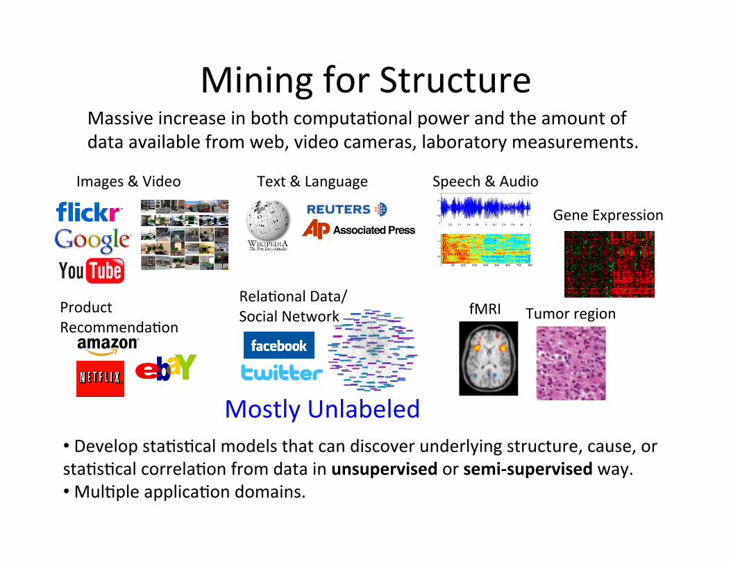
Massive increase in both computa=onal power and the amount of data available from web, video cameras, laboratory measurements.
Mining for Structure
Speech & Audio Text & Language
Product Recommenda=on
Mostly Unlabeled • Develop sta=s=cal models that can discover underlying structure, cause, or sta=s=cal correla=on from data in unsupervised or semi-‐supervised way. • Mul=ple applica=on domains.
Gene Expression
fMRI Tumor region
Images & Video
Rela=onal Data/ Social Network
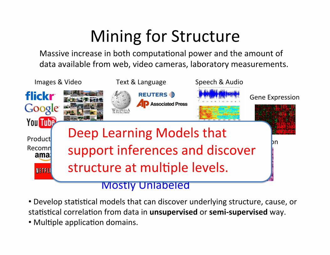
Massive increase in both computa=onal power and the amount of data available from web, video cameras, laboratory measurements.
Mining for Structure
Speech & Audio
Gene Expression
Text & Language
Product Recommenda=on
fMRI
Mostly Unlabeled • Develop sta=s=cal models that can discover underlying structure, cause, or sta=s=cal correla=on from data in unsupervised or semi-‐supervised way. • Mul=ple applica=on domains.
Tumor region Deep Learning Models that support inferences and discover structure at mul=ple levels.
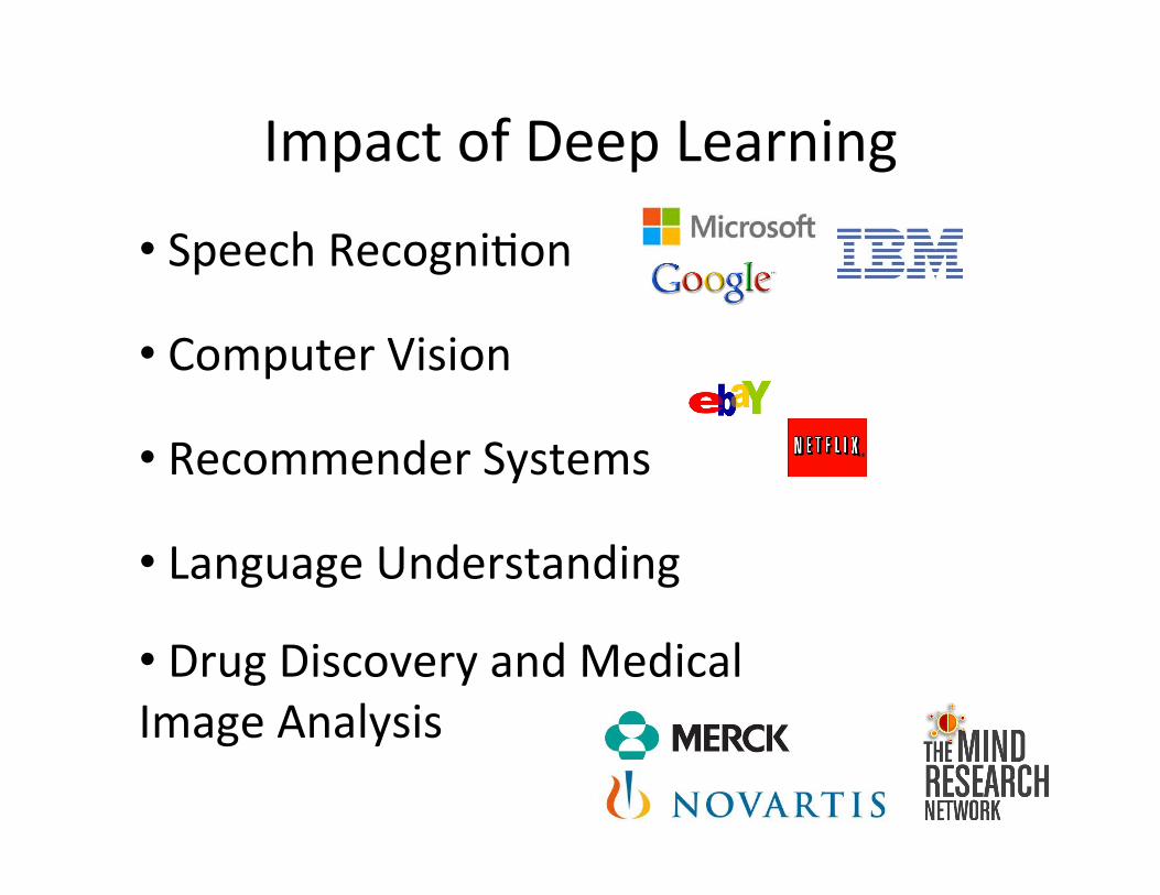
Impact of Deep Learning
• Speech Recogni=on
• Computer Vision
• Language Understanding
• Recommender Systems
• Drug Discovery and Medical Image Analysis
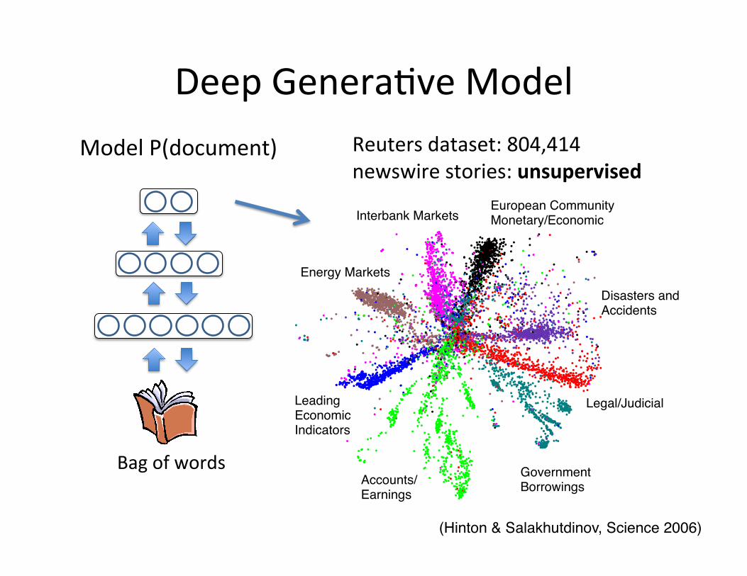
Legal/JudicialLeading Economic Indicators
European Community Monetary/Economic
Accounts/Earnings
Interbank Markets
Government Borrowings
Disasters and Accidents
Energy Markets
Model P(document)
Bag of words
Reuters dataset: 804,414 newswire stories: unsupervised
Deep Genera=ve Model
(Hinton & Salakhutdinov, Science 2006)!
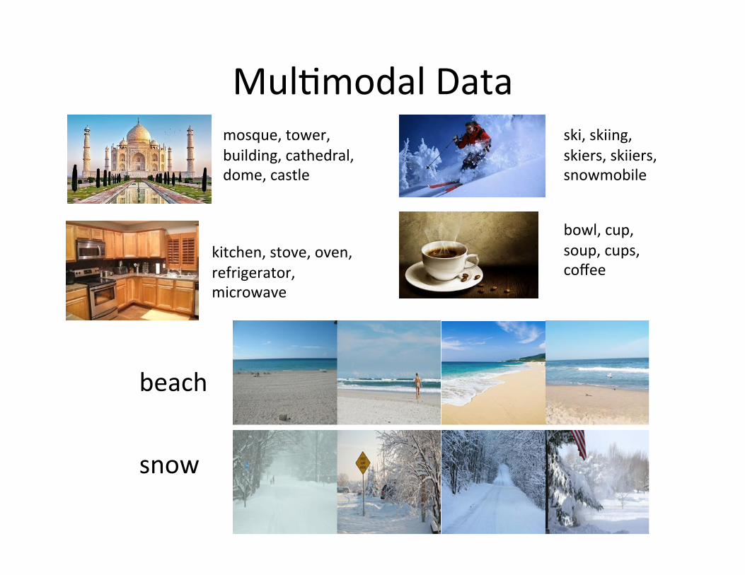
Mul=modal Data mosque, tower, building, cathedral, dome, castle
kitchen, stove, oven, refrigerator, microwave
ski, skiing, skiers, skiiers, snowmobile
bowl, cup, soup, cups, coffee
beach
snow
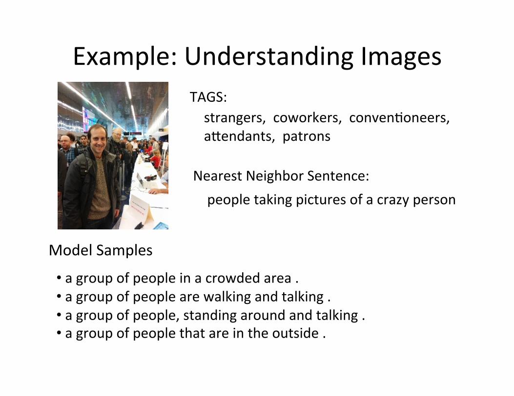
Example: Understanding Images
Model Samples
• a group of people in a crowded area . • a group of people are walking and talking . • a group of people, standing around and talking . • a group of people that are in the outside .
strangers, coworkers, conven=oneers, a[endants, patrons
TAGS:
Nearest Neighbor Sentence: people taking pictures of a crazy person

Cap=on Genera=on
Kiros et.al., TACL 2015
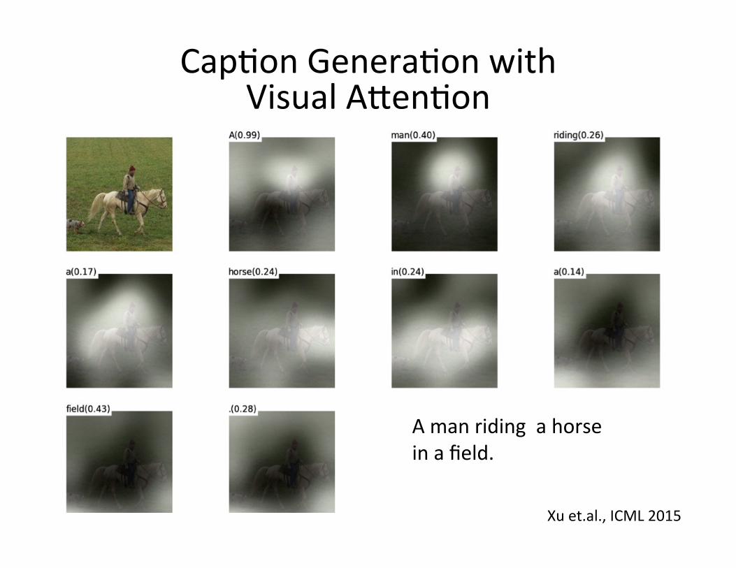
Cap=on Genera=on with Visual A[en=on
A man riding a horse in a field.
Xu et.al., ICML 2015
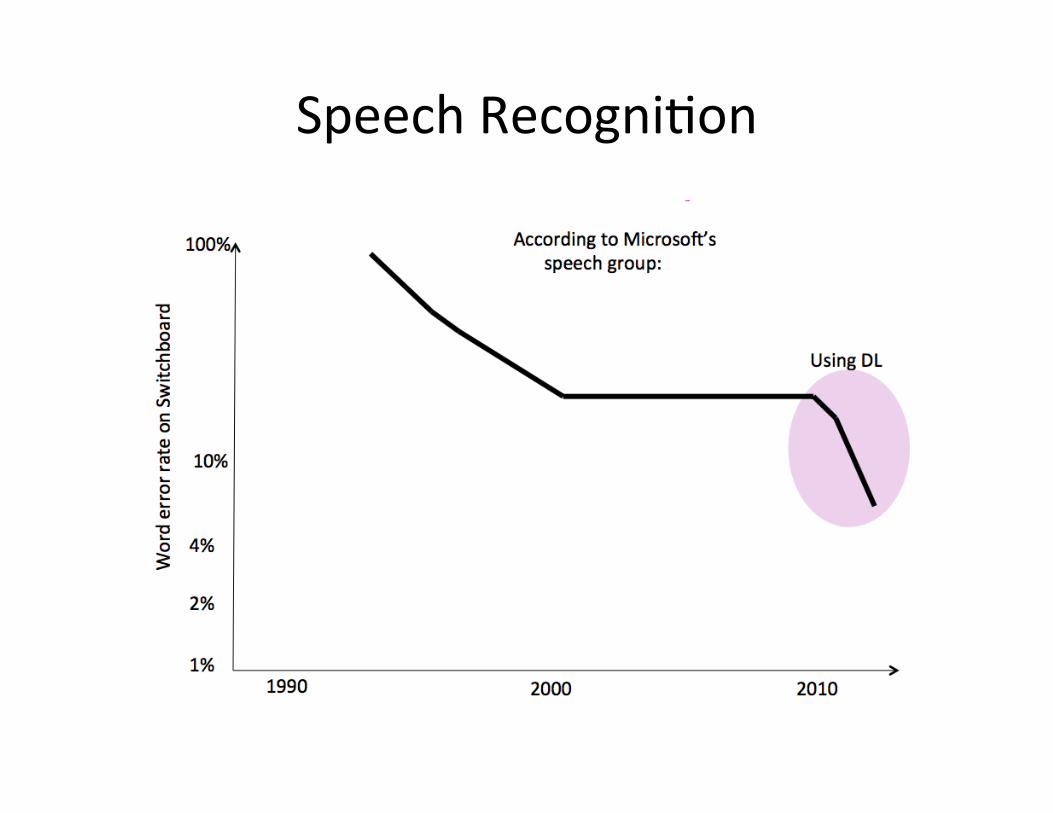
Speech Recogni=on
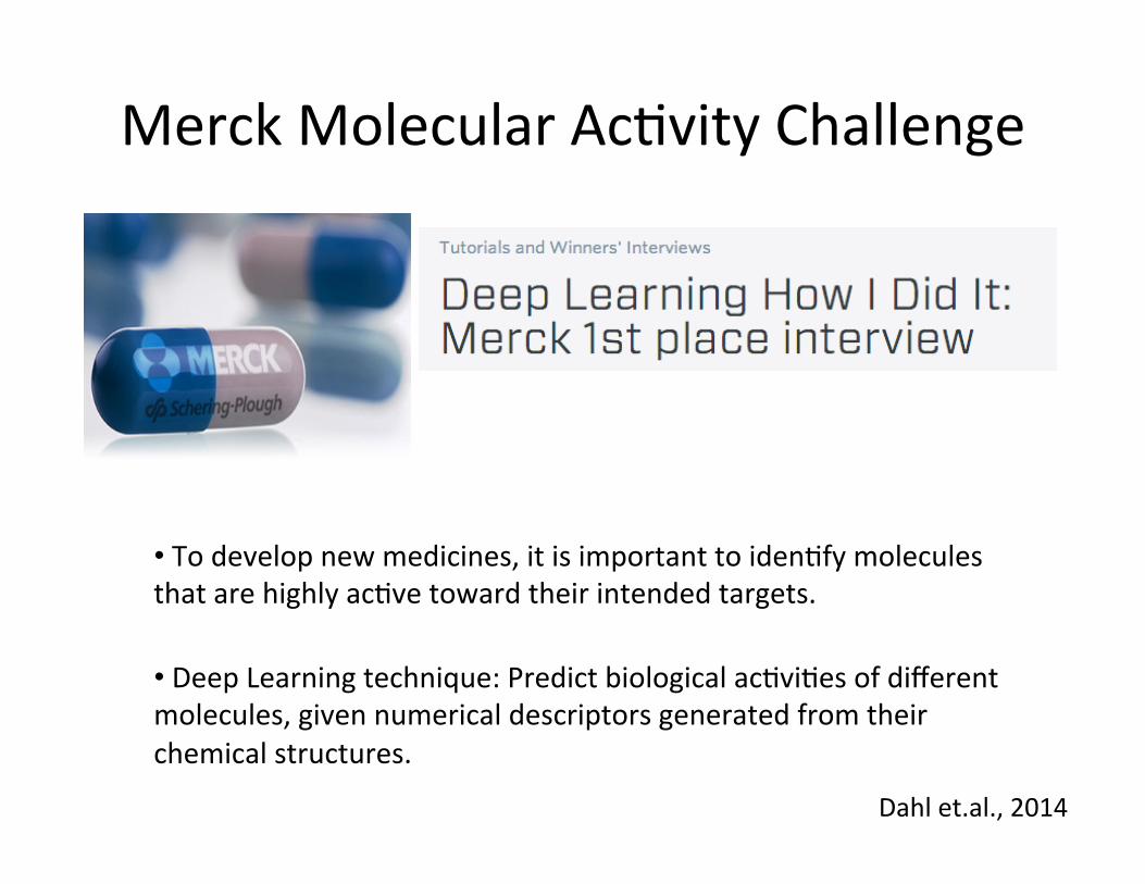
Merck Molecular Ac=vity Challenge
• Deep Learning technique: Predict biological ac=vi=es of different molecules, given numerical descriptors generated from their chemical structures.
• To develop new medicines, it is important to iden=fy molecules that are highly ac=ve toward their intended targets.
Dahl et.al., 2014
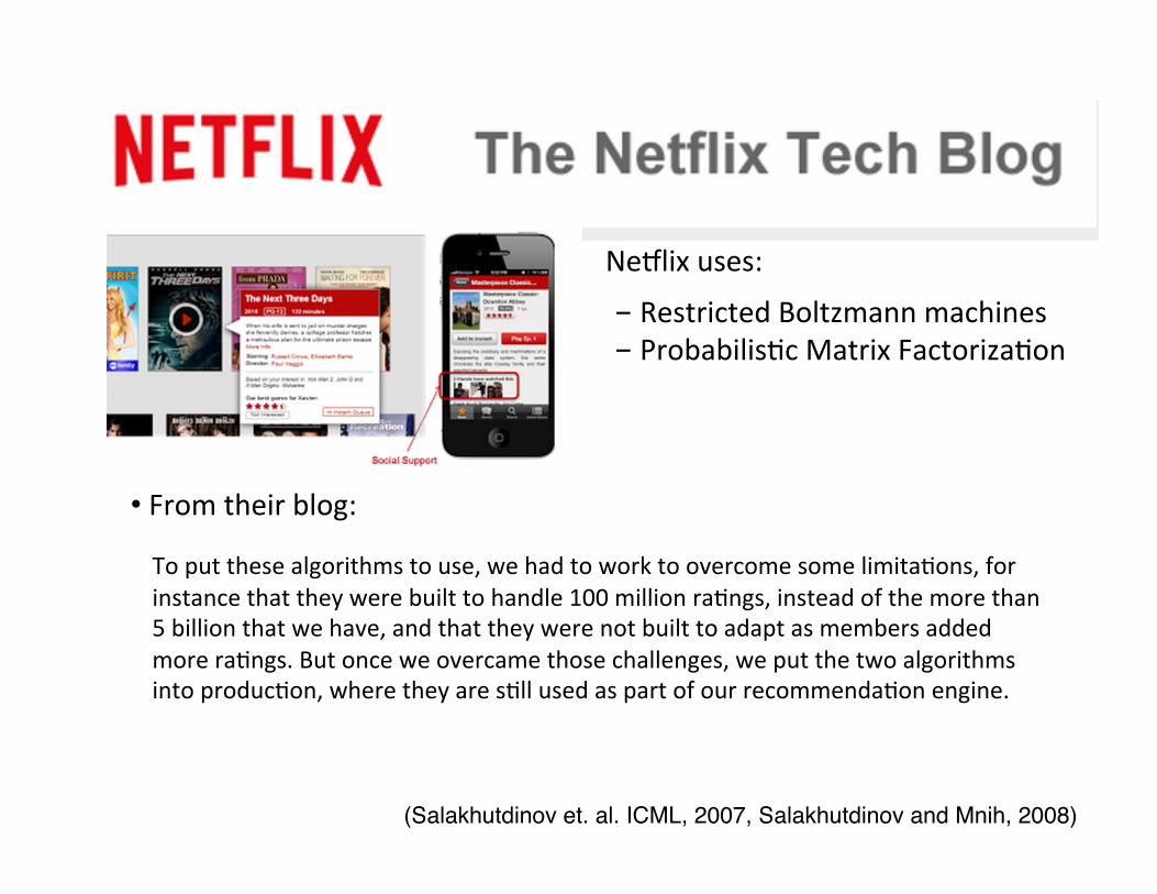
• From their blog:
- Restricted Boltzmann machines - Probabilis=c Matrix Factoriza=on
(Salakhutdinov et. al. ICML, 2007, Salakhutdinov and Mnih, 2008)!
To put these algorithms to use, we had to work to overcome some limita=ons, for instance that they were built to handle 100 million ra=ngs, instead of the more than 5 billion that we have, and that they were not built to adapt as members added more ra=ngs. But once we overcame those challenges, we put the two algorithms into produc=on, where they are s=ll used as part of our recommenda=on engine.
Neblix uses:

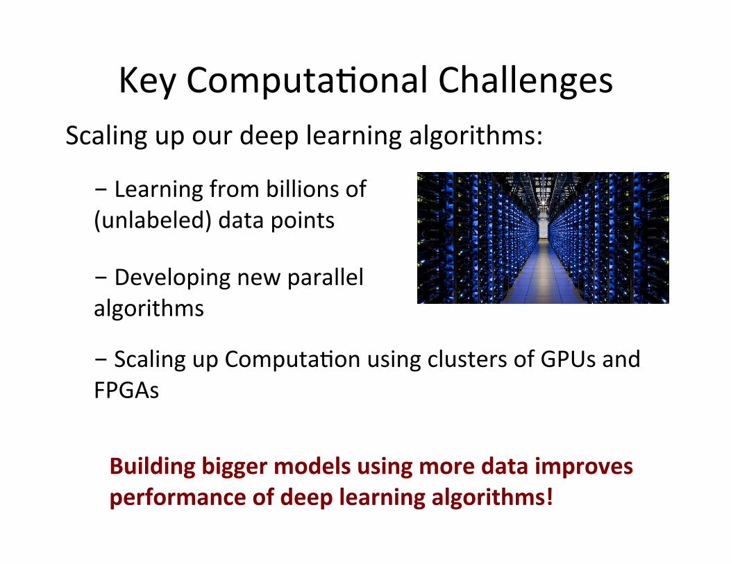
Key Computa=onal Challenges
- Learning from billions of (unlabeled) data points
- Developing new parallel algorithms
Building bigger models using more data improves performance of deep learning algorithms!
Scaling up our deep learning algorithms:
- Scaling up Computa=on using clusters of GPUs and FPGAs
Talk Roadmap
• Introduc=on, Sparse Coding, Autoencoders. • Restricted Boltzmann Machines: Learning low-‐
level features. • Deep Belief Networks • Deep Boltzmann Machines: Learning Part-‐based
Hierarchies.
Part 1: Deep Networks
Part 2: Advanced Deep Models.
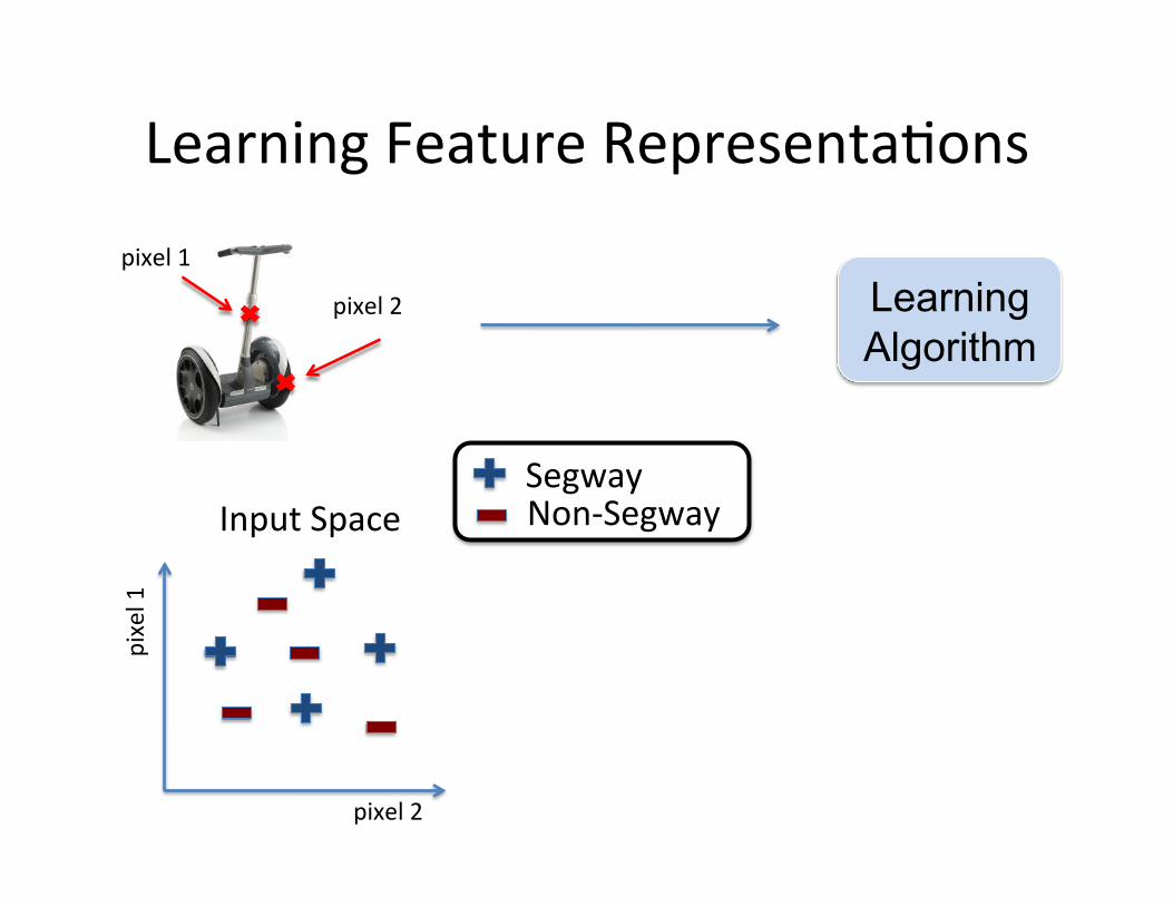
Learning Feature Representa=ons
pixel 1
pixel 2 Learning Algorithm
pixel 2
pixel 1
Segway Non-‐Segway Input Space
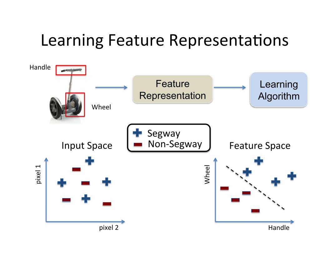
Learning Feature Representa=ons
pixel 2
pixel 1
Segway Non-‐Segway Input Space
Handle
Wheel
Learning Algorithm
Feature Representation
Handle
Whe
el
Feature Space
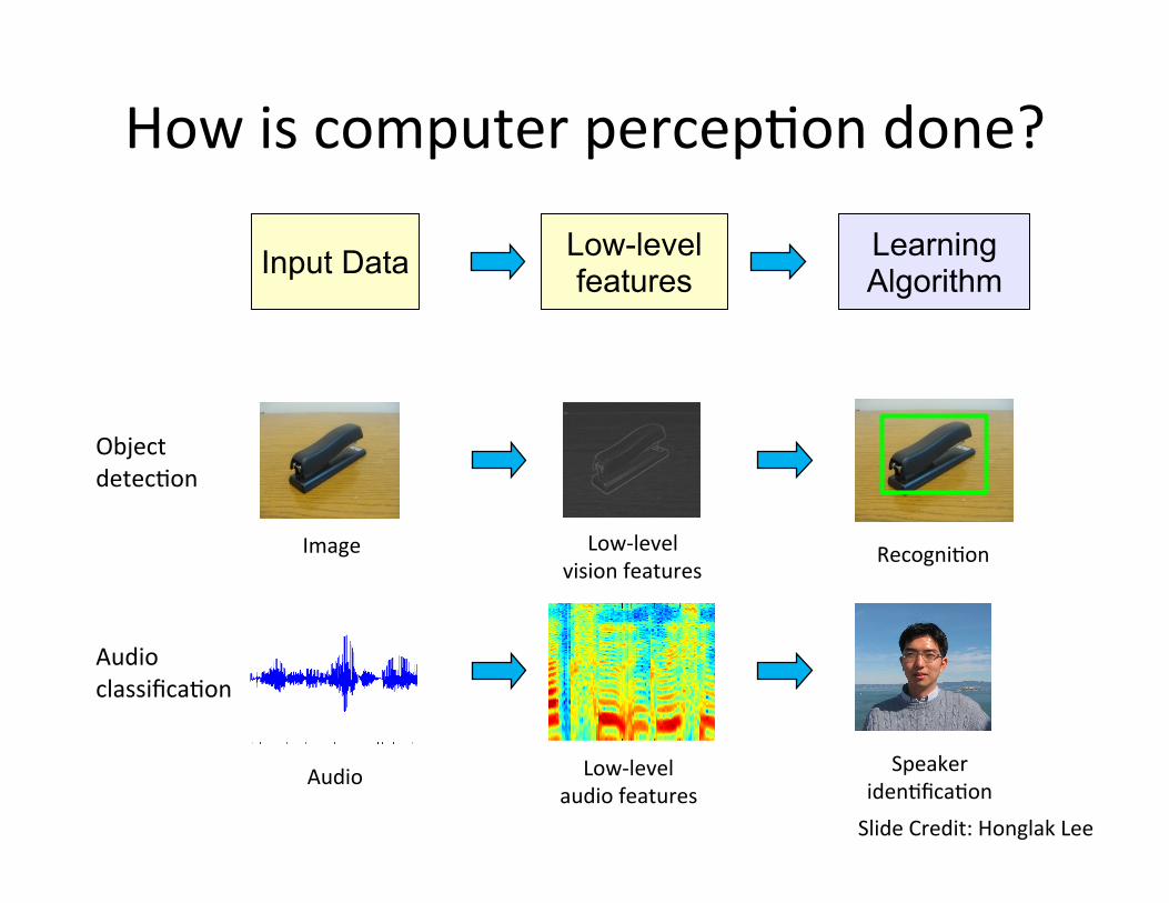
How is computer percep=on done?
Image Low-‐level vision features
Recogni=on
Object detec=on
Input Data Learning Algorithm
Low-level features
Slide Credit: Honglak Lee
Audio classifica=on
Audio Low-‐level audio features
Speaker iden=fica=on
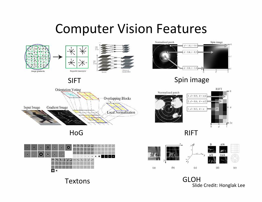
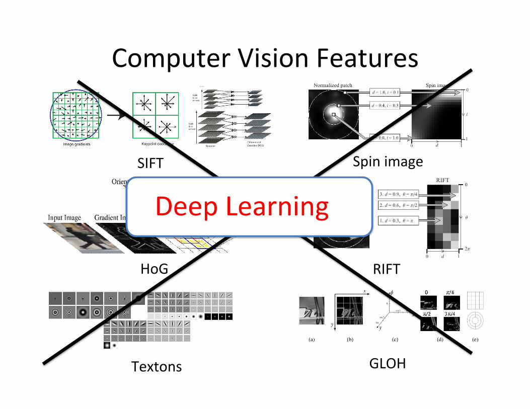
Computer Vision Features
SIFT Spin image
HoG RIFT
Textons GLOH Slide Credit: Honglak Lee
Computer Vision Features
SIFT Spin image
HoG RIFT
Textons GLOH
Deep Learning
ZCR
Spectrogram MFCC
Rolloff Flux
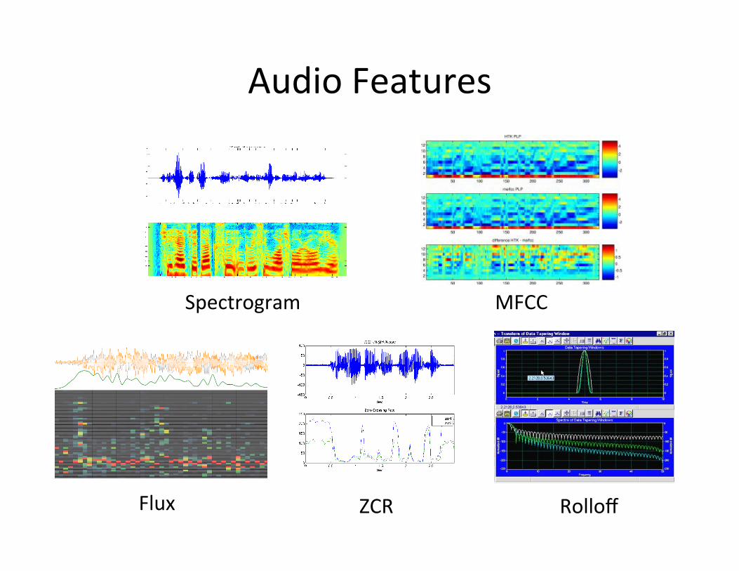
Audio Features

Audio Features
ZCR
Spectrogram MFCC
Rolloff Flux
Deep Learning
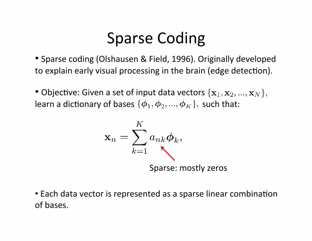
Sparse Coding • Sparse coding (Olshausen & Field, 1996). Originally developed to explain early visual processing in the brain (edge detec=on).
• Objec=ve: Given a set of input data vectors learn a dic=onary of bases such that:
• Each data vector is represented as a sparse linear combina=on of bases.
Sparse: mostly zeros
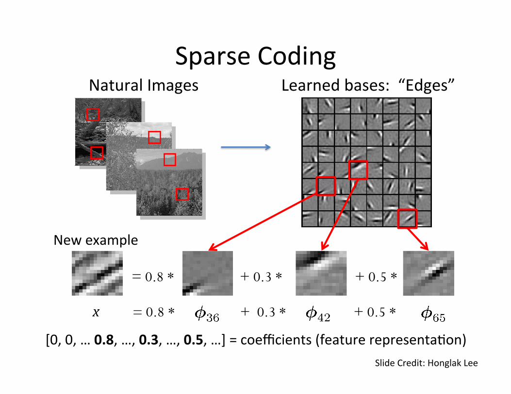
Learned bases: “Edges” Natural Images
[0, 0, … 0.8, …, 0.3, …, 0.5, …] = coefficients (feature representa=on)
= 0.8 * + 0.3 * + 0.5 *
New example
Sparse Coding
x = 0.8 * + 0.3 *
+ 0.5 *
Slide Credit: Honglak Lee
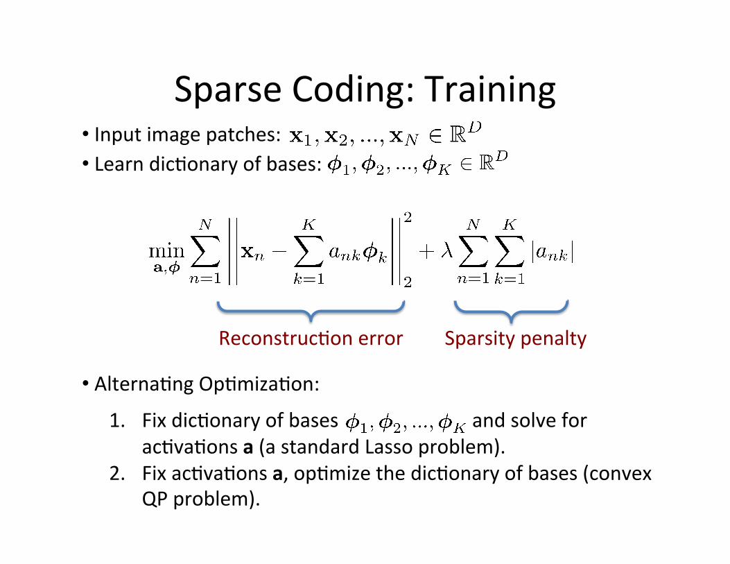
Sparse Coding: Training • Input image patches: • Learn dic=onary of bases:
Reconstruc=on error Sparsity penalty
• Alterna=ng Op=miza=on:
1. Fix dic=onary of bases and solve for ac=va=ons a (a standard Lasso problem).
2. Fix ac=va=ons a, op=mize the dic=onary of bases (convex QP problem).

Sparse Coding: Tes=ng Time • Input: a new image patch x* , and K learned bases • Output: sparse representa=on a of an image patch x*.
= 0.8 * + 0.3 * + 0.5 *
x* = 0.8 * + 0.3 *
+ 0.5 *
[0, 0, … 0.8, …, 0.3, …, 0.5, …] = coefficients (feature representa=on)
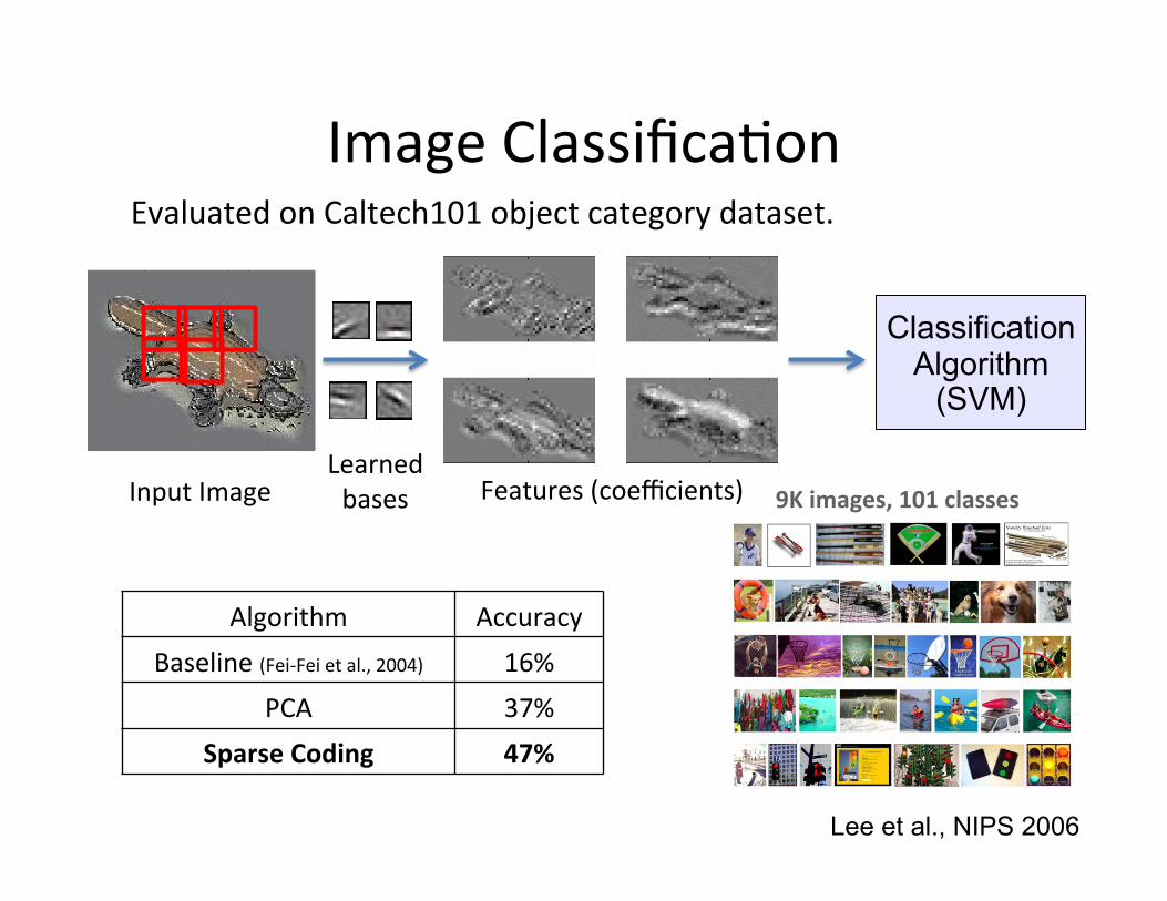
Evaluated on Caltech101 object category dataset.
Classification Algorithm
(SVM)
Algorithm Accuracy Baseline (Fei-‐Fei et al., 2004) 16%
PCA 37% Sparse Coding 47%
Input Image Features (coefficients) Learned bases
Image Classifica=on
9K images, 101 classes
Lee et al., NIPS 2006
g(a)
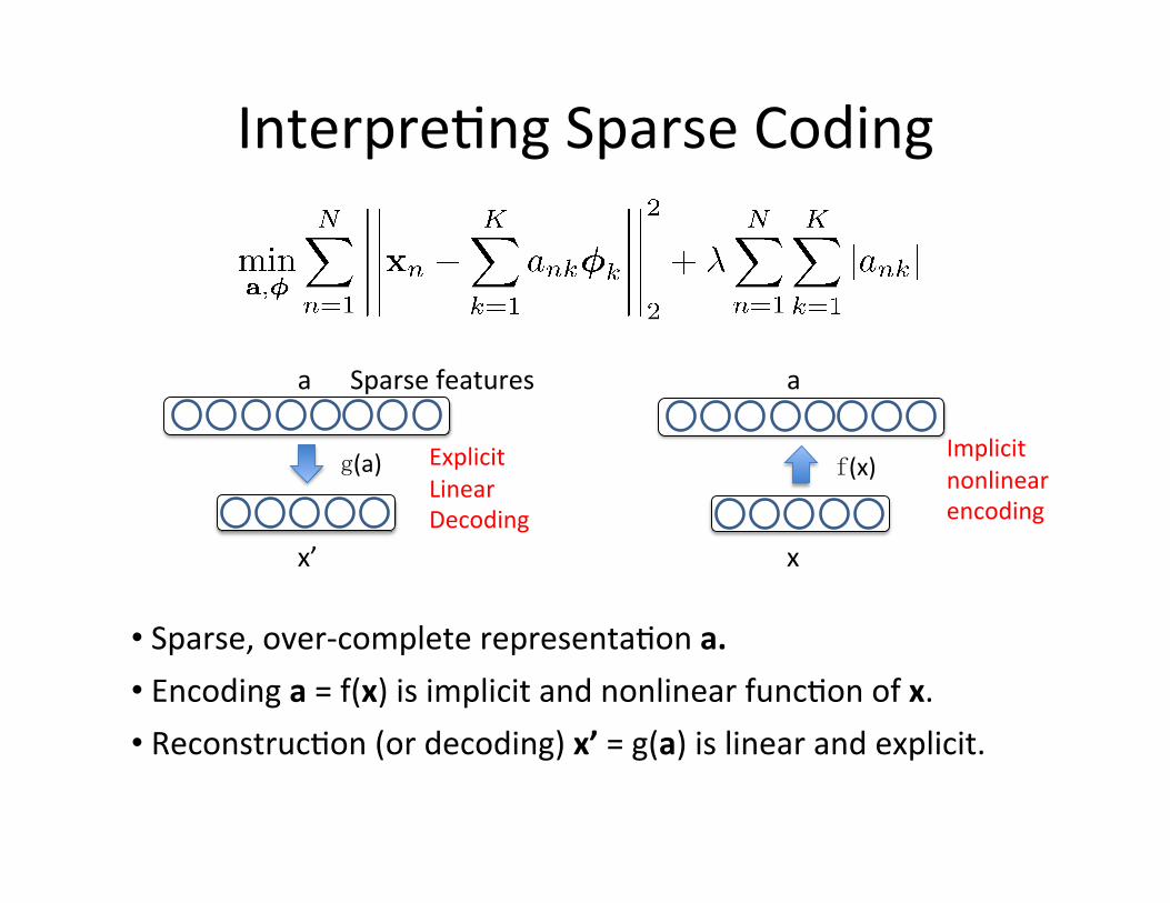
Interpre=ng Sparse Coding
x’
Explicit Linear Decoding
a
f(x) Implicit nonlinear encoding
x
a
• Sparse, over-‐complete representa=on a. • Encoding a = f(x) is implicit and nonlinear func=on of x. • Reconstruc=on (or decoding) x’ = g(a) is linear and explicit.
Sparse features
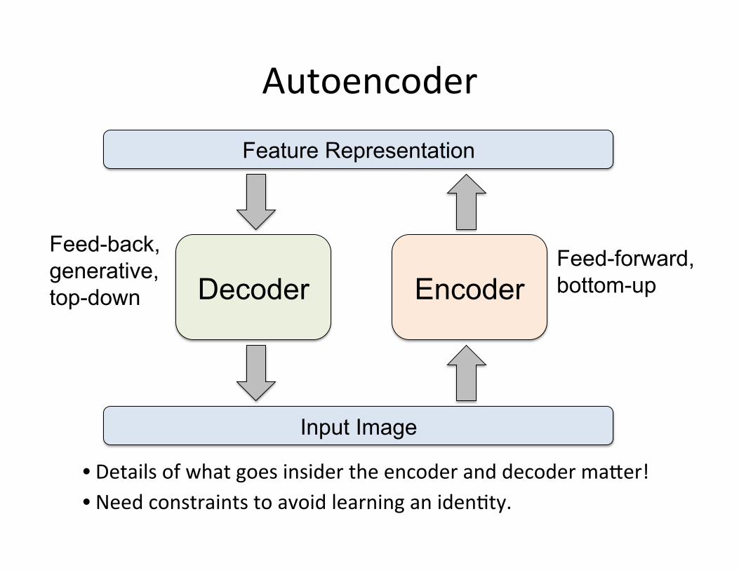
Autoencoder
Encoder Decoder
Input Image
Feature Representation
Feed-back, generative, top-down path
Feed-forward, bottom-up
• Details of what goes insider the encoder and decoder ma[er! • Need constraints to avoid learning an iden=ty.
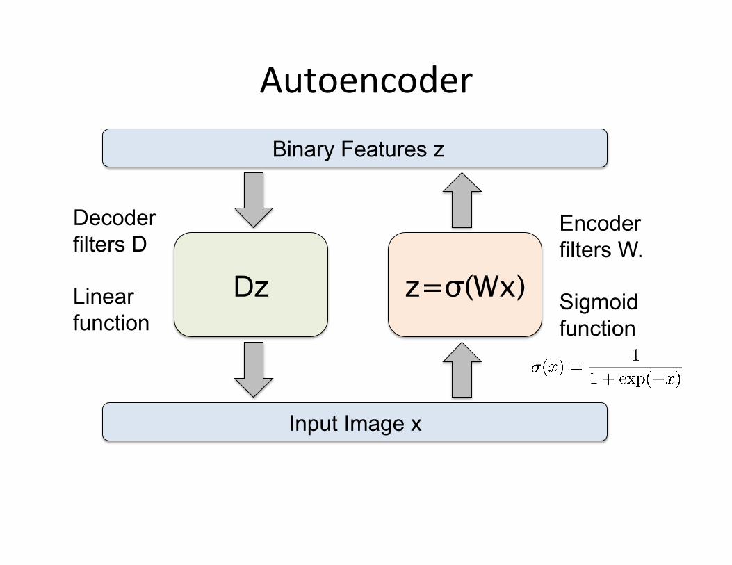
Autoencoder
z=σ(Wx) Dz
Input Image x
Binary Features z
Decoder filters D
Linear function path
Encoder filters W.
Sigmoid function

Autoencoder • An autoencoder with D inputs, D outputs, and K hidden units, with K<D.
• Given an input x, its reconstruc=on is given by:
Encoder
z=σ(Wx) Dz
Input Image x
Binary Features z
Decoder
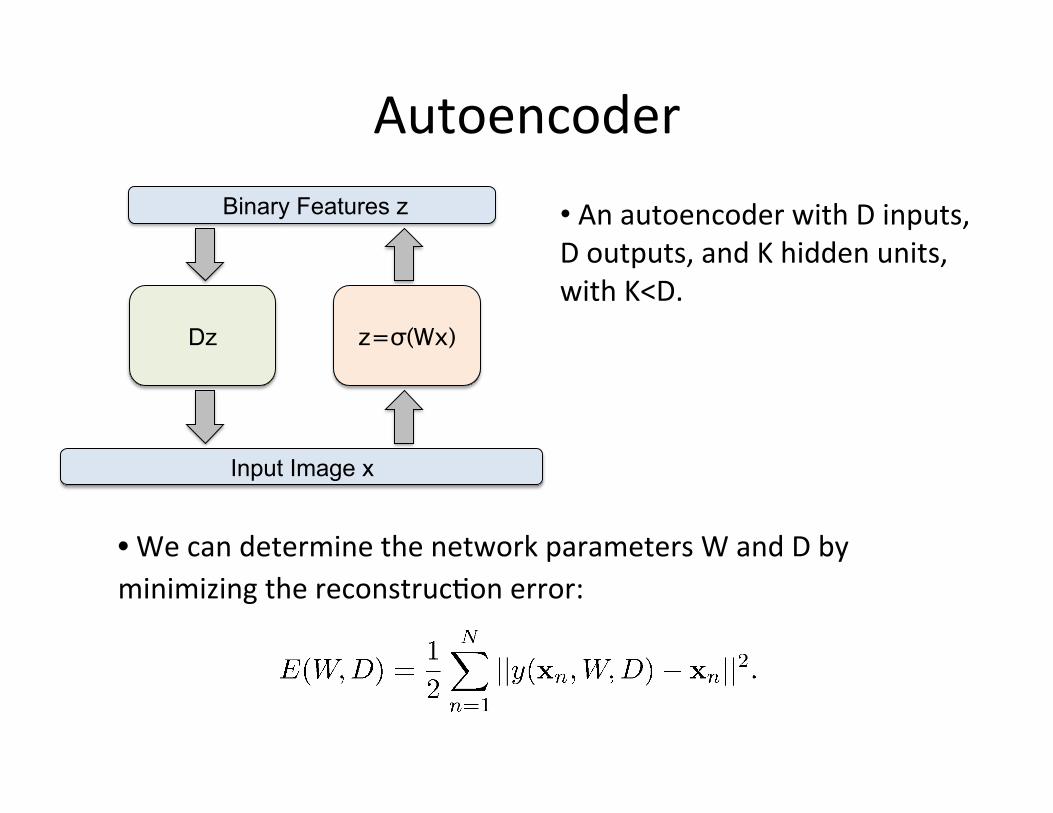
Autoencoder • An autoencoder with D inputs, D outputs, and K hidden units, with K<D.
z=σ(Wx) Dz
Input Image x
Binary Features z
• We can determine the network parameters W and D by minimizing the reconstruc=on error:
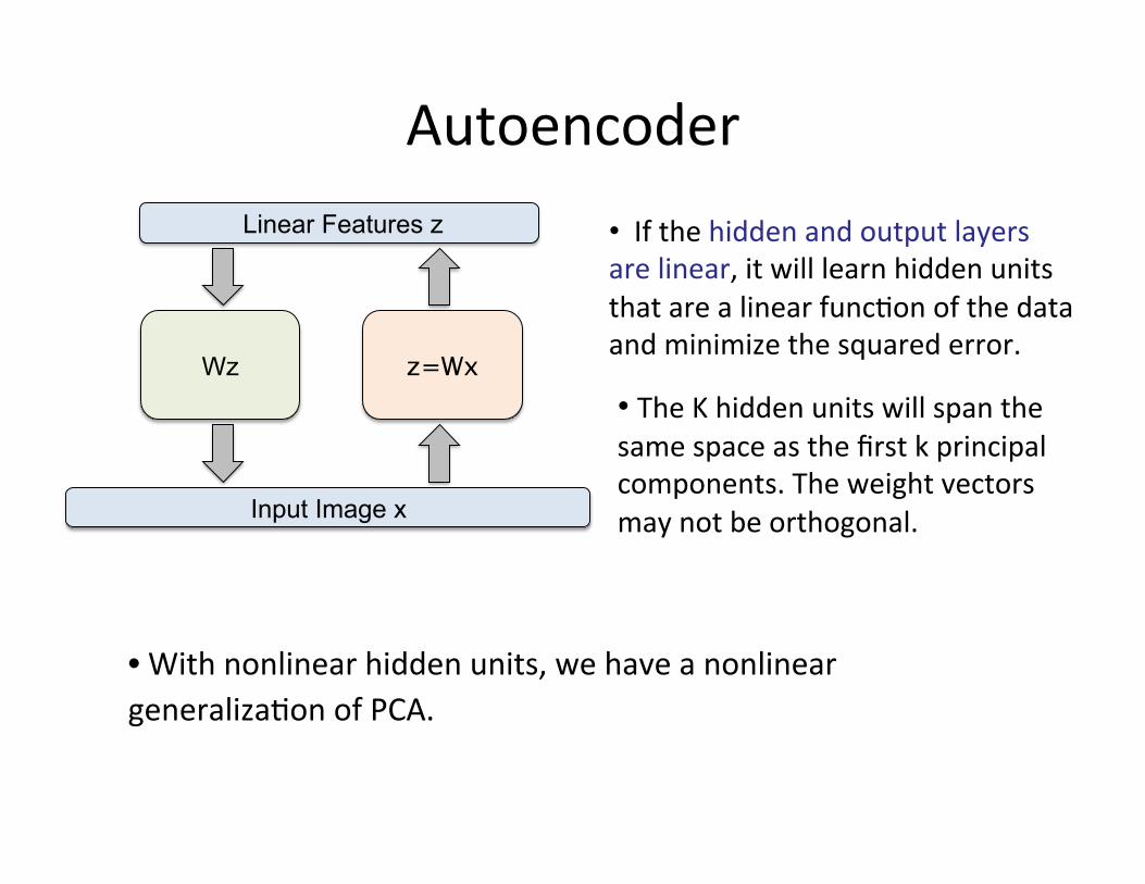
Autoencoder • If the hidden and output layers are linear, it will learn hidden units that are a linear func=on of the data and minimize the squared error.
• The K hidden units will span the same space as the first k principal components. The weight vectors may not be orthogonal.
z=Wx Wz
Input Image x
Linear Features z
• With nonlinear hidden units, we have a nonlinear generaliza=on of PCA.
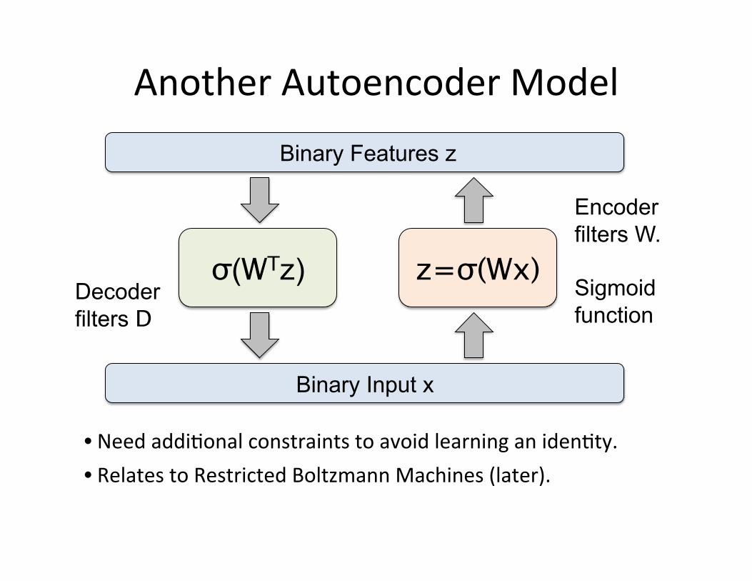
Another Autoencoder Model
z=σ(Wx) σ(WTz)
Binary Input x
Binary Features z
Decoder filters D path
Encoder filters W.
Sigmoid function
• Relates to Restricted Boltzmann Machines (later). • Need addi=onal constraints to avoid learning an iden=ty.
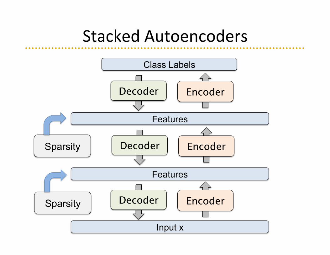
Stacked Autoencoders
Input x
Features
Encoder Decoder
Class Labels
Encoder Decoder
Sparsity
Features
Encoder Decoder Sparsity
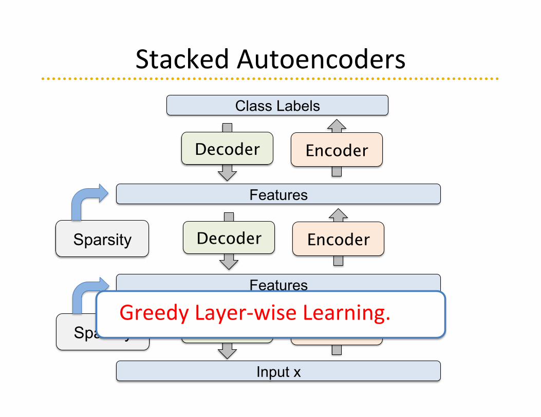
Stacked Autoencoders
Input x
Features
Encoder Decoder
Features
Class Labels
Encoder Decoder
Encoder Decoder
Sparsity
Sparsity
Greedy Layer-‐wise Learning.
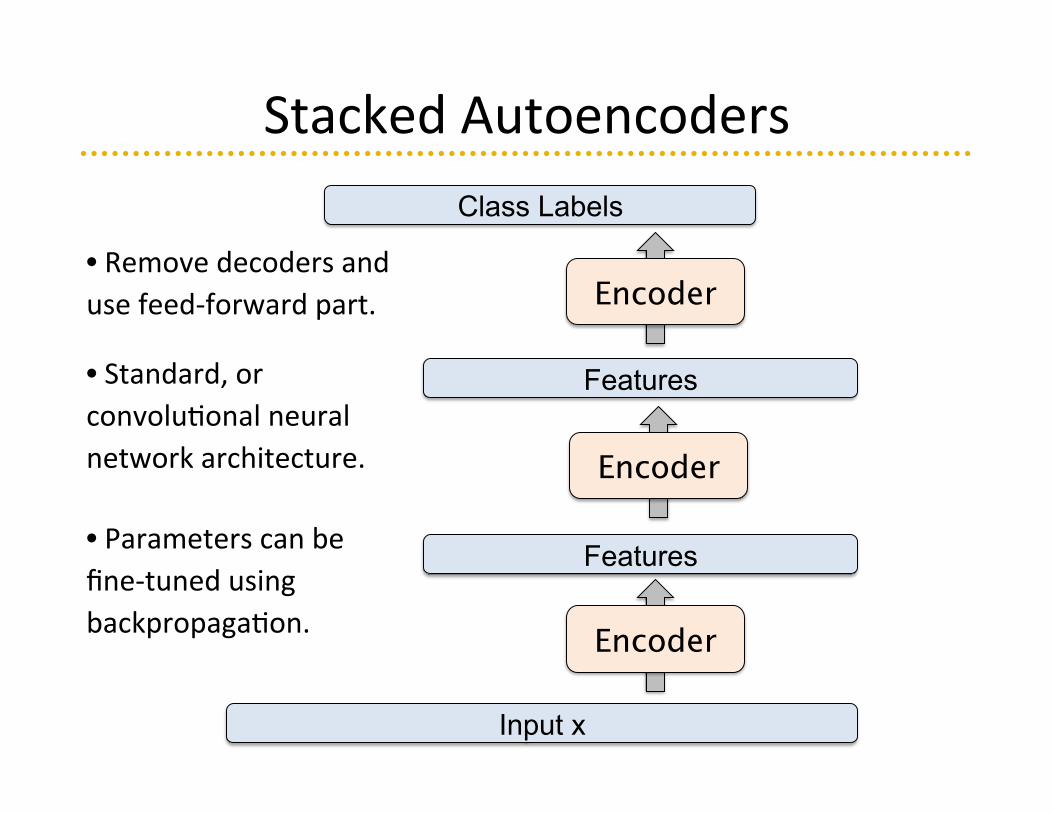
Stacked Autoencoders
Input x
Features
Encoder
Features
Class Labels
Encoder
Encoder • Remove decoders and use feed-‐forward part.
• Standard, or convolu=onal neural network architecture.
• Parameters can be fine-‐tuned using backpropaga=on.
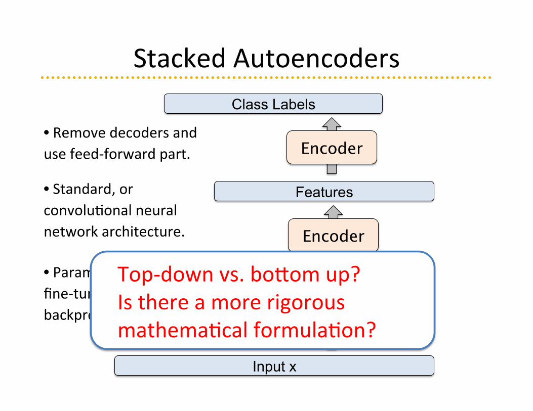
Stacked Autoencoders
Input x
Features
Encoder
Features
Class Labels
Encoder
Encoder • Remove decoders and use feed-‐forward part.
• Standard, or convolu=onal neural network architecture.
• Parameters can be fine-‐tuned using backpropaga=on.
Top-‐down vs. bo[om up? Is there a more rigorous mathema=cal formula=on?
Talk Roadmap
• Introduc=on, Sparse Coding, Autoencoders. • Restricted Boltzmann Machines: Learning low-‐
level features. • Deep Belief Networks • Deep Boltzmann Machines: Learning Part-‐based
Hierarchies.
Part 1: Deep Networks
Part 2: Advanced Deep Models.
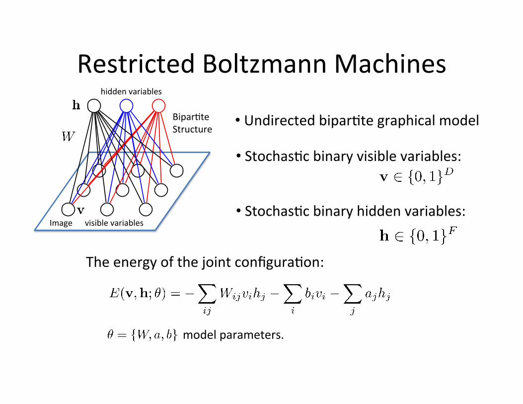
Restricted Boltzmann Machines
The energy of the joint configura=on:
model parameters.
• Stochas=c binary hidden variables:
• Stochas=c binary visible variables:
Image visible variables
hidden variables
Bipar=te Structure
• Undirected bipar=te graphical model
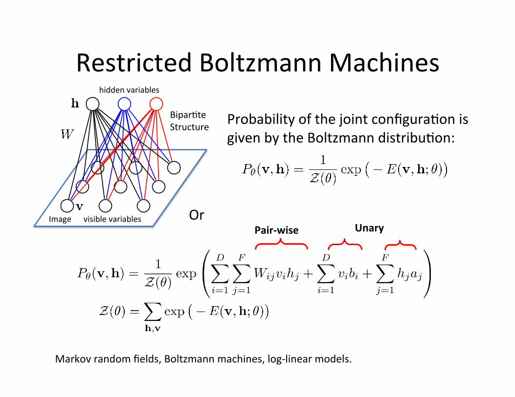
Restricted Boltzmann Machines
Probability of the joint configura=on is given by the Boltzmann distribu=on:
Markov random fields, Boltzmann machines, log-‐linear models.
Image visible variables
hidden variables
Bipar=te Structure
Pair-‐wise Unary Or

Restricted Boltzmann Machines
Restricted: No interac=on between hidden variables
Inferring the distribu=on over the hidden variables is easy:
Factorizes: Easy to compute
Image visible variables
hidden variables
Bipar=te Structure
Similarly:
Markov random fields, Boltzmann machines, log-‐linear models.
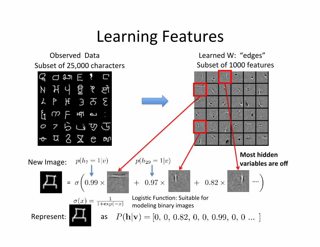
Learned W: “edges” Subset of 1000 features
Learning Features
= ….
New Image:
Logis=c Func=on: Suitable for modeling binary images
Most hidden variables are off
Observed Data Subset of 25,000 characters
Represent: as
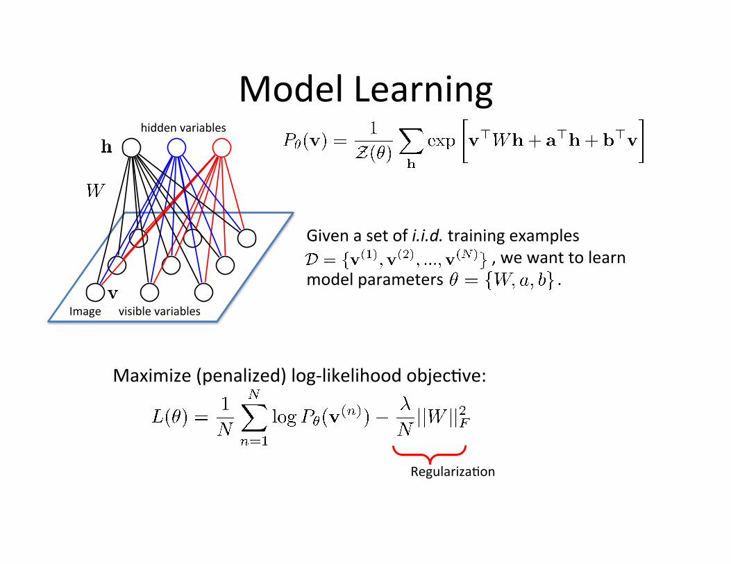
Model Learning
Image visible variables
hidden variables
Given a set of i.i.d. training examples , we want to learn
model parameters .
Maximize (penalized) log-‐likelihood objec=ve:
Regulariza=on
Model Learning
Image visible variables
hidden variables
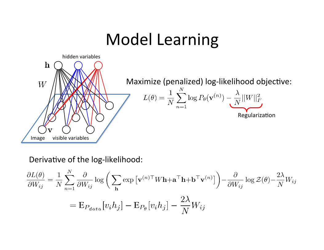
Maximize (penalized) log-‐likelihood objec=ve:
Regulariza=on
Deriva=ve of the log-‐likelihood:
Model Learning
Image visible variables
hidden variables
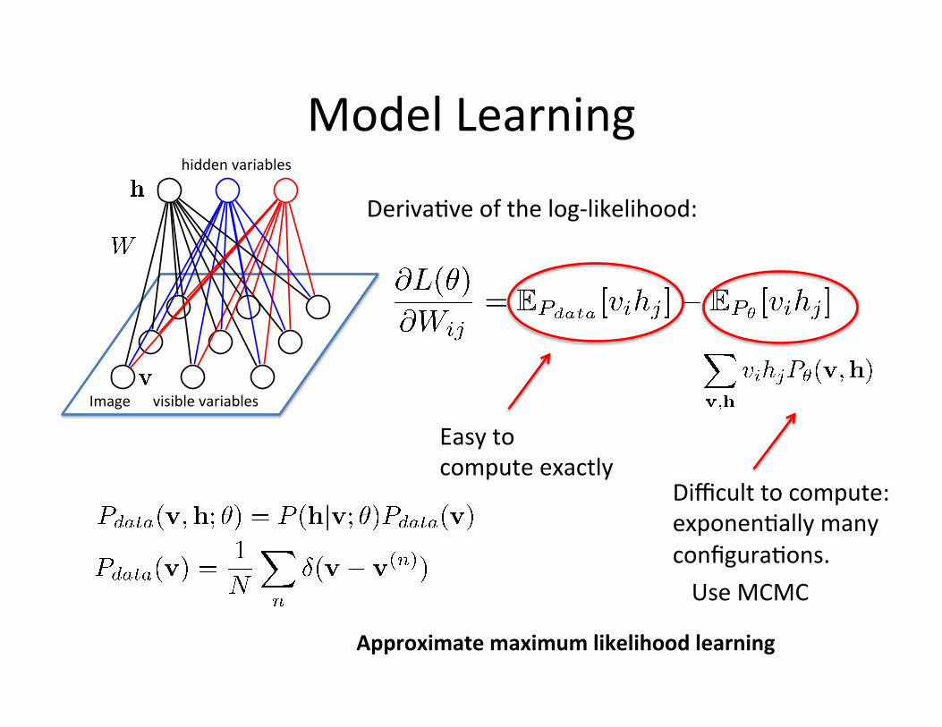
Deriva=ve of the log-‐likelihood:
Easy to compute exactly
Difficult to compute: exponen=ally many configura=ons.
Approximate maximum likelihood learning
Use MCMC
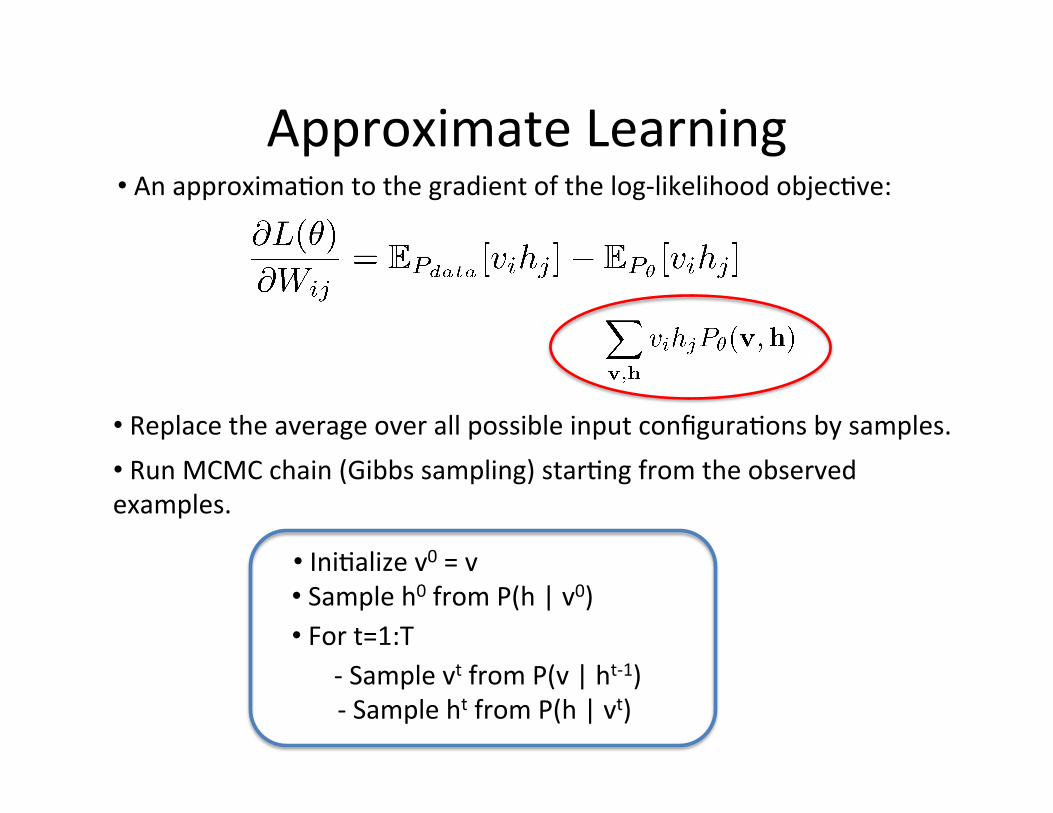
Approximate Learning • An approxima=on to the gradient of the log-‐likelihood objec=ve:
• Run MCMC chain (Gibbs sampling) star=ng from the observed examples.
• Replace the average over all possible input configura=ons by samples.
• Ini=alize v0 = v • Sample h0 from P(h | v0) • For t=1:T
-‐ Sample vt from P(v | ht-‐1) -‐ Sample ht from P(h | vt)
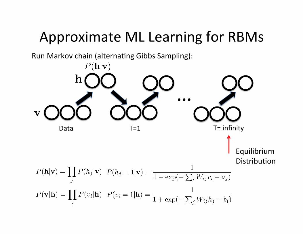
Approximate ML Learning for RBMs Run Markov chain (alterna=ng Gibbs Sampling):
… Data T=1 T= infinity
Equilibrium Distribu=on
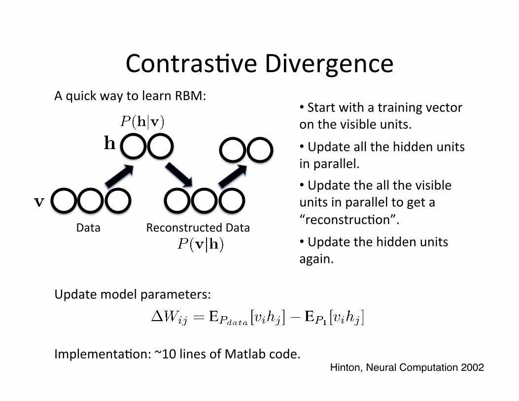
Contras=ve Divergence A quick way to learn RBM:
Data Reconstructed Data
Hinton, Neural Computation 2002!
• Start with a training vector on the visible units.
• Update the hidden units again.
• Update all the hidden units in parallel. • Update the all the visible units in parallel to get a “reconstruc=on”.
Update model parameters:
Implementa=on: ~10 lines of Matlab code.

Gaussian-‐Bernoulli RBM:
• Stochas=c real-‐valued visible variables • Stochas=c binary hidden variables • Bipar=te connec=ons.
Pair-‐wise Unary
Image visible variables
hidden variables
RBMs for Real-‐valued Data

Pair-‐wise Unary
Image visible variables
hidden variables
RBMs for Real-‐valued Data
Learned features (out of 10,000) 4 million unlabelled images

RBMs for Real-‐valued Data
= 0.9 * + 0.8 * + 0.6 * … New Image
Learned features (out of 10,000) 4 million unlabelled images
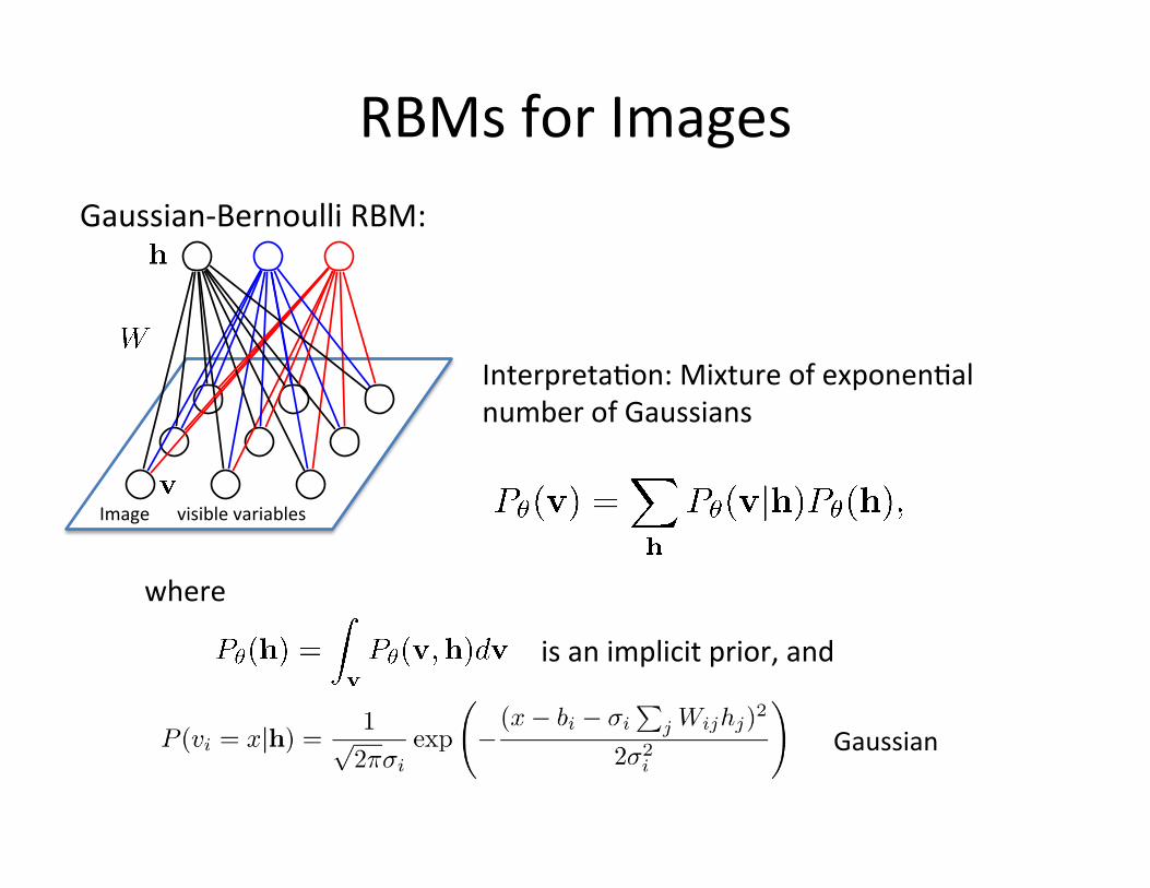
RBMs for Images Gaussian-‐Bernoulli RBM:
Interpreta=on: Mixture of exponen=al number of Gaussians
Gaussian
Image visible variables
where
is an implicit prior, and
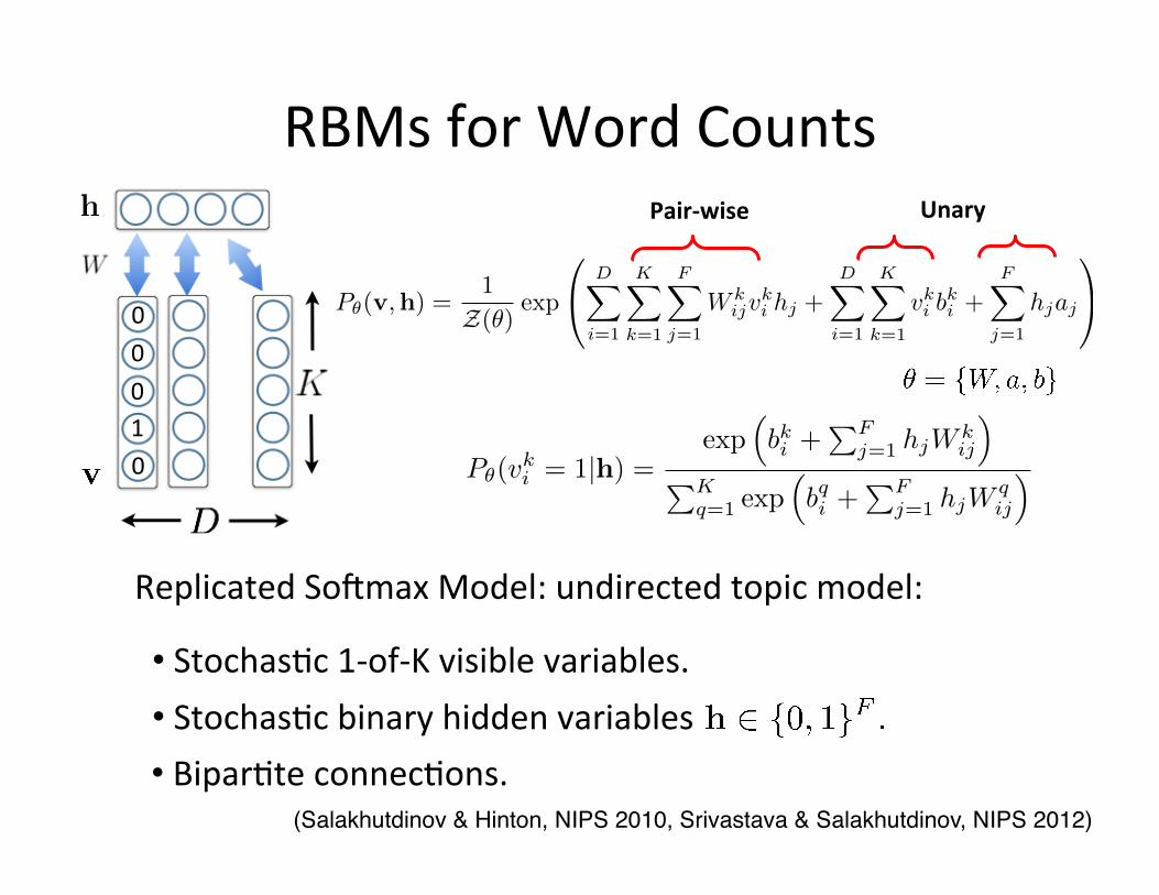
RBMs for Word Counts
Replicated So8max Model: undirected topic model:
• Stochas=c 1-‐of-‐K visible variables. • Stochas=c binary hidden variables • Bipar=te connec=ons.
Pair-‐wise Unary
P✓(v,h) =1
Z(✓)exp
0
@DX
i=1
KX
k=1
FX
j=1
W kijv
ki hj +
DX
i=1
KX
k=1
vki bki +
FX
j=1
hjaj
1
A
P✓(vki = 1|h) =
exp
⇣bki +
PFj=1 hjW k
ij
⌘
PKq=1 exp
⇣bqi +
PFj=1 hjW
qij
⌘
0 0 1 0
0
(Salakhutdinov & Hinton, NIPS 2010, Srivastava & Salakhutdinov, NIPS 2012)!

RBMs for Word Counts Pair-‐wise Unary
P✓(v,h) =1
Z(✓)exp
0
@DX
i=1
KX
k=1
FX
j=1
W kijv
ki hj +
DX
i=1
KX
k=1
vki bki +
FX
j=1
hjaj
1
A
P✓(vki = 1|h) =
exp
⇣bki +
PFj=1 hjW k
ij
⌘
PKq=1 exp
⇣bqi +
PFj=1 hjW
qij
⌘
0 0 1 0
0
Learned features: ``topics’’
russian russia moscow yeltsin soviet
clinton house president bill congress
computer system product so8ware develop
trade country import world economy
stock wall street point dow
Reuters dataset: 804,414 unlabeled newswire stories Bag-‐of-‐Words

RBMs for Word Counts
One-‐step reconstruc=on from the Replicated So8max model.
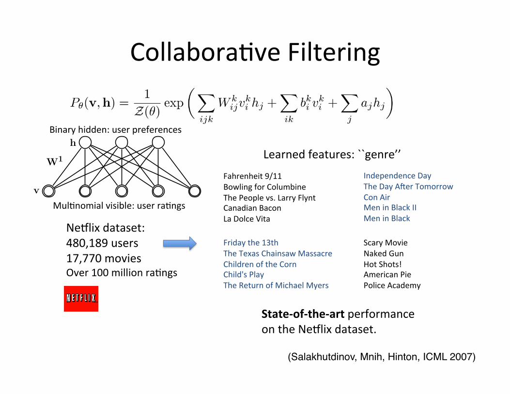
Learned features: ``genre’’
Fahrenheit 9/11 Bowling for Columbine The People vs. Larry Flynt Canadian Bacon La Dolce Vita
Independence Day The Day A8er Tomorrow Con Air Men in Black II Men in Black
Friday the 13th The Texas Chainsaw Massacre Children of the Corn Child's Play The Return of Michael Myers
Scary Movie Naked Gun Hot Shots! American Pie Police Academy
Neblix dataset: 480,189 users 17,770 movies Over 100 million ra=ngs
State-‐of-‐the-‐art performance on the Neblix dataset.
Collabora=ve Filtering
(Salakhutdinov, Mnih, Hinton, ICML 2007)!
h
v
W1
Mul=nomial visible: user ra=ngs
Binary hidden: user preferences
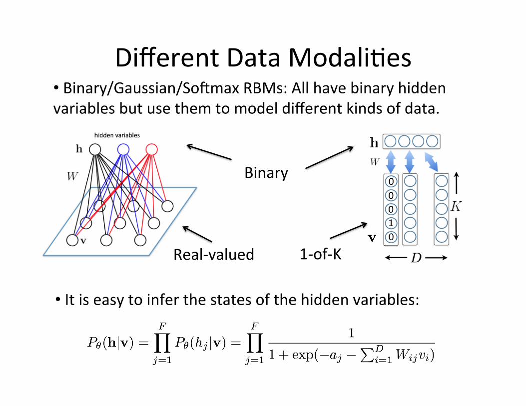
Different Data Modali=es
• It is easy to infer the states of the hidden variables:
• Binary/Gaussian/So8max RBMs: All have binary hidden variables but use them to model different kinds of data.
Binary
Real-‐valued 1-‐of-‐K
0 0 1 0
0
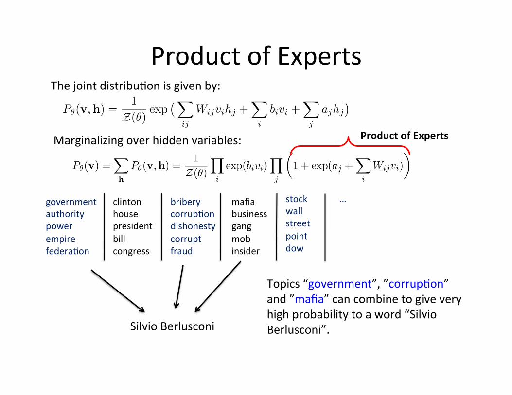
Product of Experts
Marginalizing over hidden variables: Product of Experts
The joint distribu=on is given by:
Silvio Berlusconi
government authority power empire federa=on
clinton house president bill congress
bribery corrup=on dishonesty corrupt fraud
mafia business gang mob insider
stock wall street point dow
…
Topics “government”, ”corrup=on” and ”mafia” can combine to give very high probability to a word “Silvio Berlusconi”.
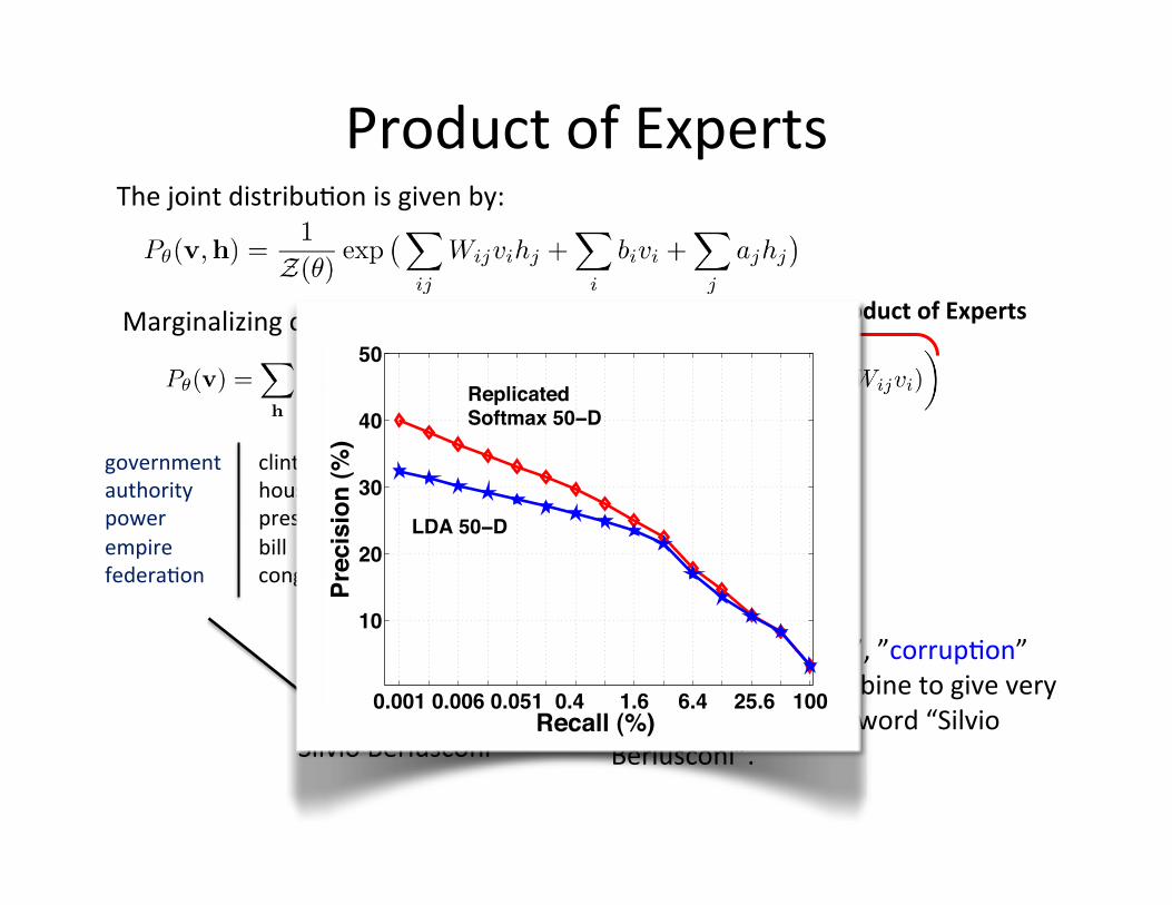
0.001 0.006 0.051 0.4 1.6 6.4 25.6 100
10
20
30
40
50
Recall (%)
Prec
isio
n (%
)
Replicated Softmax 50−D
LDA 50−D
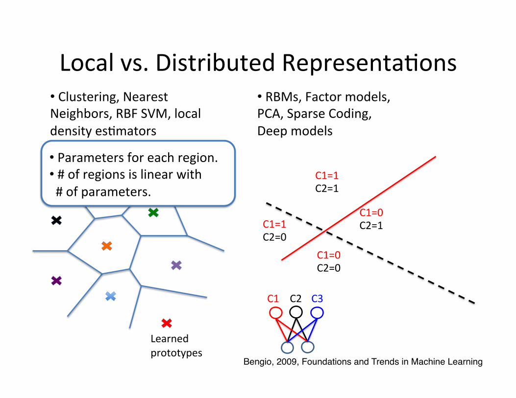
Local vs. Distributed Representa=ons • Clustering, Nearest Neighbors, RBF SVM, local density es=mators
Learned prototypes
Local regions C1=1
C1=0
C2=1
C2=1 C1=1 C2=0
C1=0 C2=0
• RBMs, Factor models, PCA, Sparse Coding, Deep models
C2 C1 C3
• Parameters for each region. • # of regions is linear with # of parameters.
Bengio, 2009, Foundations and Trends in Machine Learning!

Local vs. Distributed Representa=ons • Clustering, Nearest Neighbors, RBF SVM, local density es=mators
Learned prototypes
Local regions
C3=0
C1=1
C1=0
C3=0 C3=0
C2=1
C2=1 C1=1 C2=0
C1=0 C2=0 C3=0
C1=1 C2=1 C3=1
C1=0 C2=1 C3=1
C1=0 C2=0 C3=1
• RBMs, Factor models, PCA, Sparse Coding, Deep models
• Parameters for each region. • # of regions is linear with # of parameters.
C2 C1 C3
Bengio, 2009, Foundations and Trends in Machine Learning!

Local vs. Distributed Representa=ons • Clustering, Nearest Neighbors, RBF SVM, local density es=mators
Learned prototypes
Local regions
C3=0
C1=1
C1=0
C3=0 C3=0
C2=1
C2=1 C1=1 C2=0
C1=0 C2=0 C3=0
C1=1 C2=1 C3=1
C1=0 C2=1 C3=1
C1=0 C2=0 C3=1
• RBMs, Factor models, PCA, Sparse Coding, Deep models
• Parameters for each region. • # of regions is linear with # of parameters.
• Each parameter affects many regions, not just local. • # of regions grows (roughly) exponen=ally in # of parameters.
C2 C1 C3
Bengio, 2009, Foundations and Trends in Machine Learning!

Mul=ple Applica=on Domains
Same learning algorithm -‐-‐ mul=ple input domains.
Limita=ons on the types of structure that can be represented by a single layer of low-‐level features!
• Video • Collabora=ve Filtering / Matrix Factoriza=on • Text/Documents • Natural Images
• Mo=on Capture • Speech Percep=on
Talk Roadmap
• Introduc=on, Sparse Coding, Autoencoders. • Restricted Boltzmann Machines: Learning low-‐
level features. • Deep Belief Networks • Deep Boltzmann Machines: Learning Part-‐based
Hierarchies.
Part 1: Deep Networks
Part 2: Advanced Deep Models.
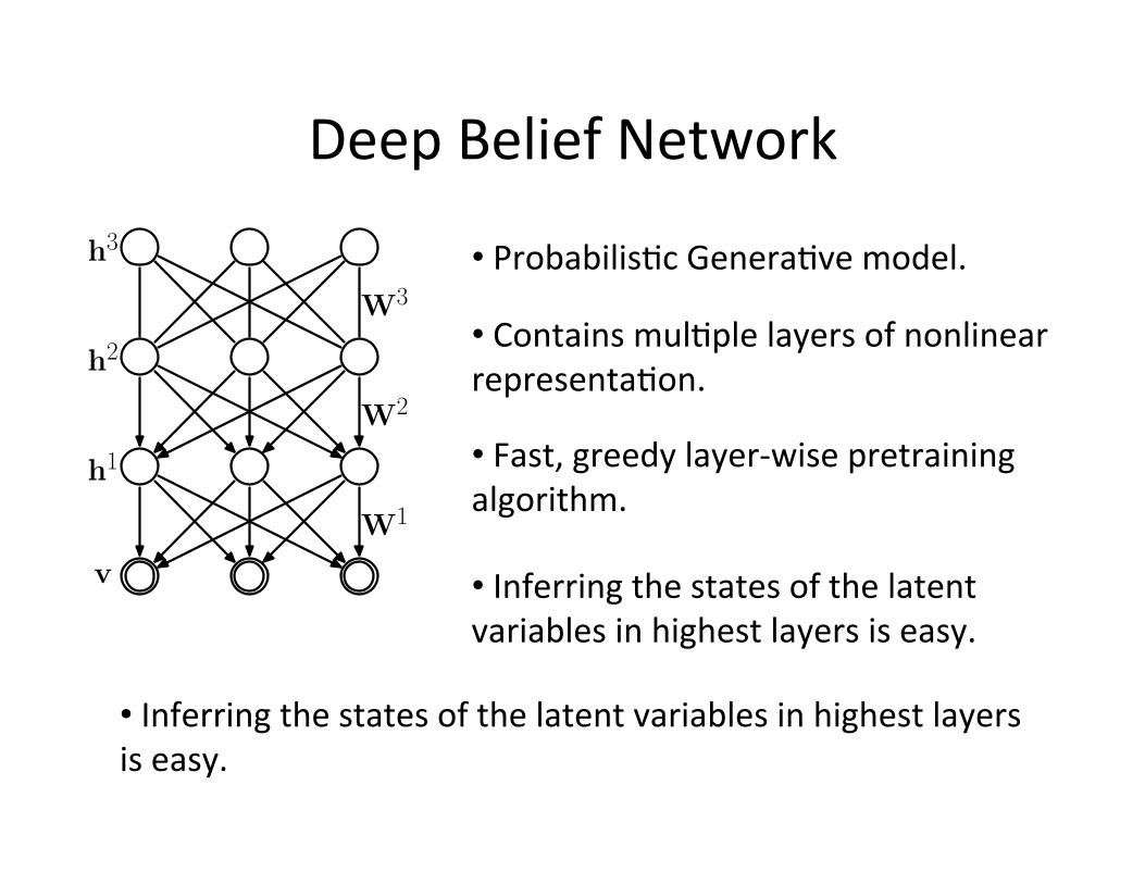
Deep Belief Network
• Probabilis=c Genera=ve model. h3
h2
h1
v
W3
W2
W1
• Contains mul=ple layers of nonlinear representa=on.
• Fast, greedy layer-‐wise pretraining algorithm.
• Inferring the states of the latent variables in highest layers is easy.
• Inferring the states of the latent variables in highest layers is easy.

Image
Low-‐level features: Edges
Input: Pixels
Built from unlabeled inputs.
Deep Belief Network
(Hinton et.al. Neural Computation 2006)!
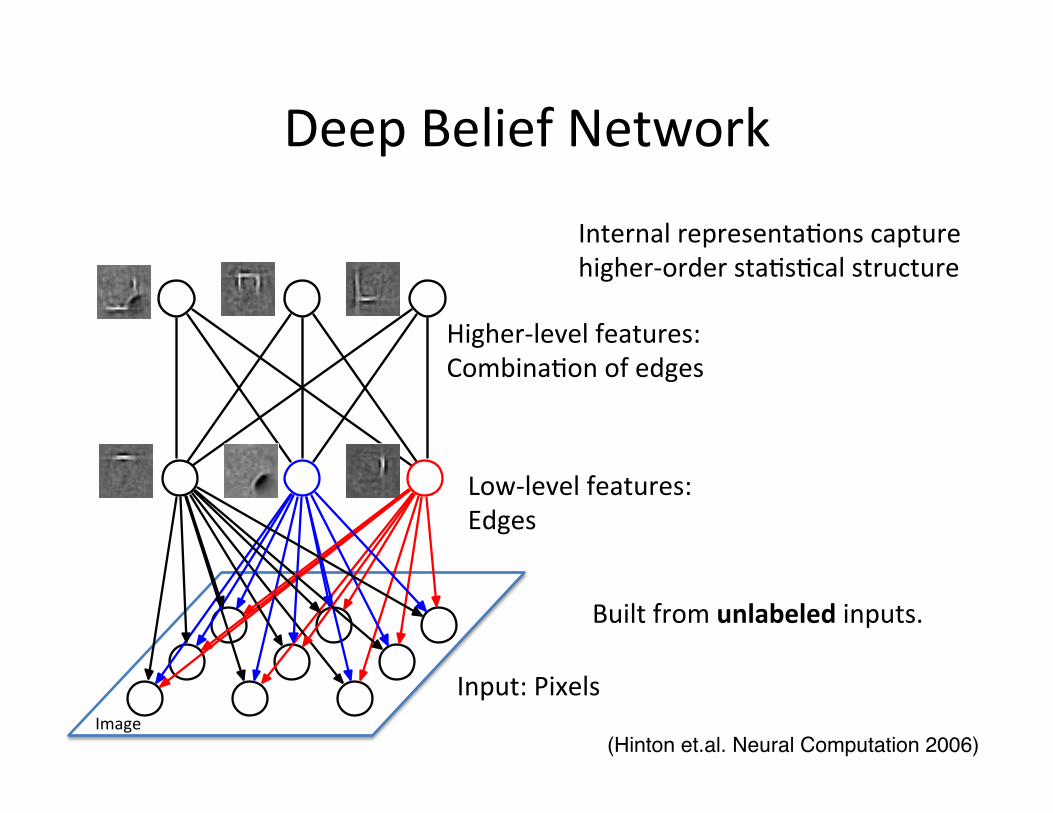
Image
Higher-‐level features: Combina=on of edges
Low-‐level features: Edges
Input: Pixels
Built from unlabeled inputs.
Deep Belief Network
Internal representa=ons capture higher-‐order sta=s=cal structure
(Hinton et.al. Neural Computation 2006)!
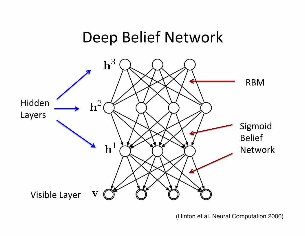
Deep Belief Network
Hidden Layers
Visible Layer
RBM
Sigmoid Belief Network
(Hinton et.al. Neural Computation 2006)!

Deep Belief Network
RBM
Sigmoid Belief Network
The joint probability distribu=on factorizes:
Deep Belief Network
RBM Sigmoid Belief Network
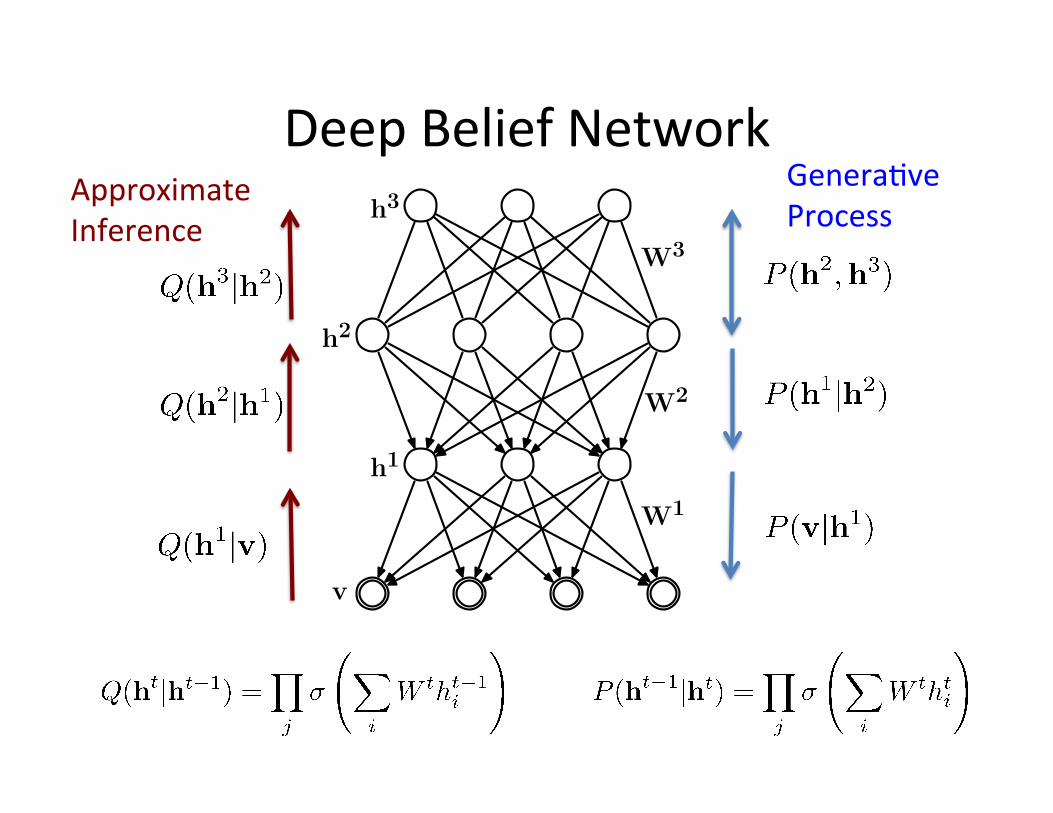
Deep Belief Network Genera=ve Process
Approximate Inference
v
h2
h1
h3
W1
W3
W2
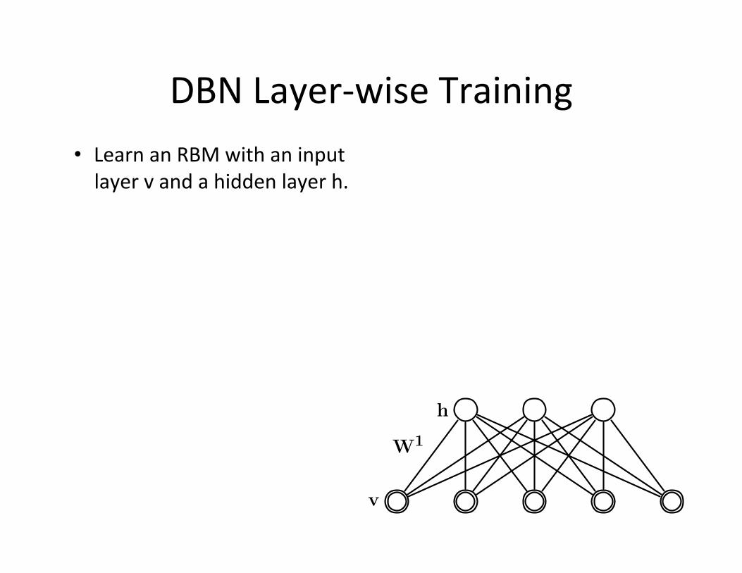
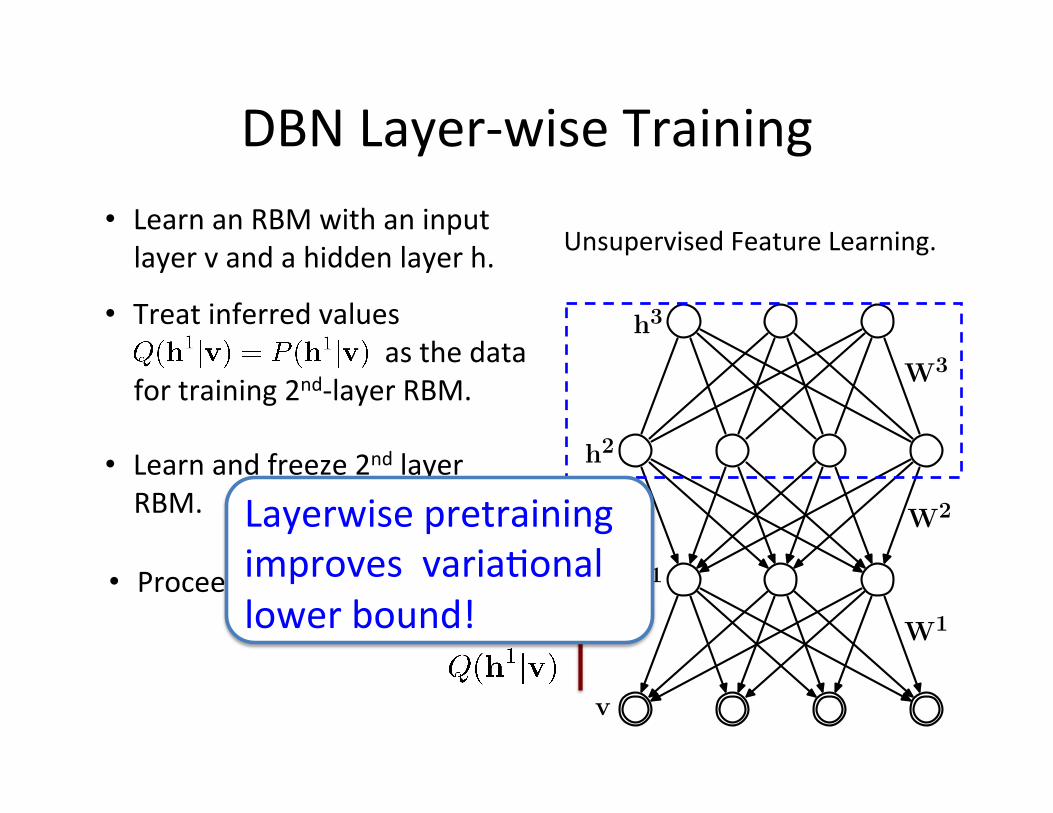
DBN Layer-‐wise Training • Learn an RBM with an input layer v and a hidden layer h.
h
v
W1

DBN Layer-‐wise Training
h1
h2
v
W1
W1⊤
• Learn an RBM with an input layer v and a hidden layer h.
• Treat inferred values as the data
for training 2nd-‐layer RBM.
• Learn and freeze 2nd layer RBM.
DBN Layer-‐wise Training
v
h2
h1
h3
W1
W3
W2
• Proceed to the next layer.
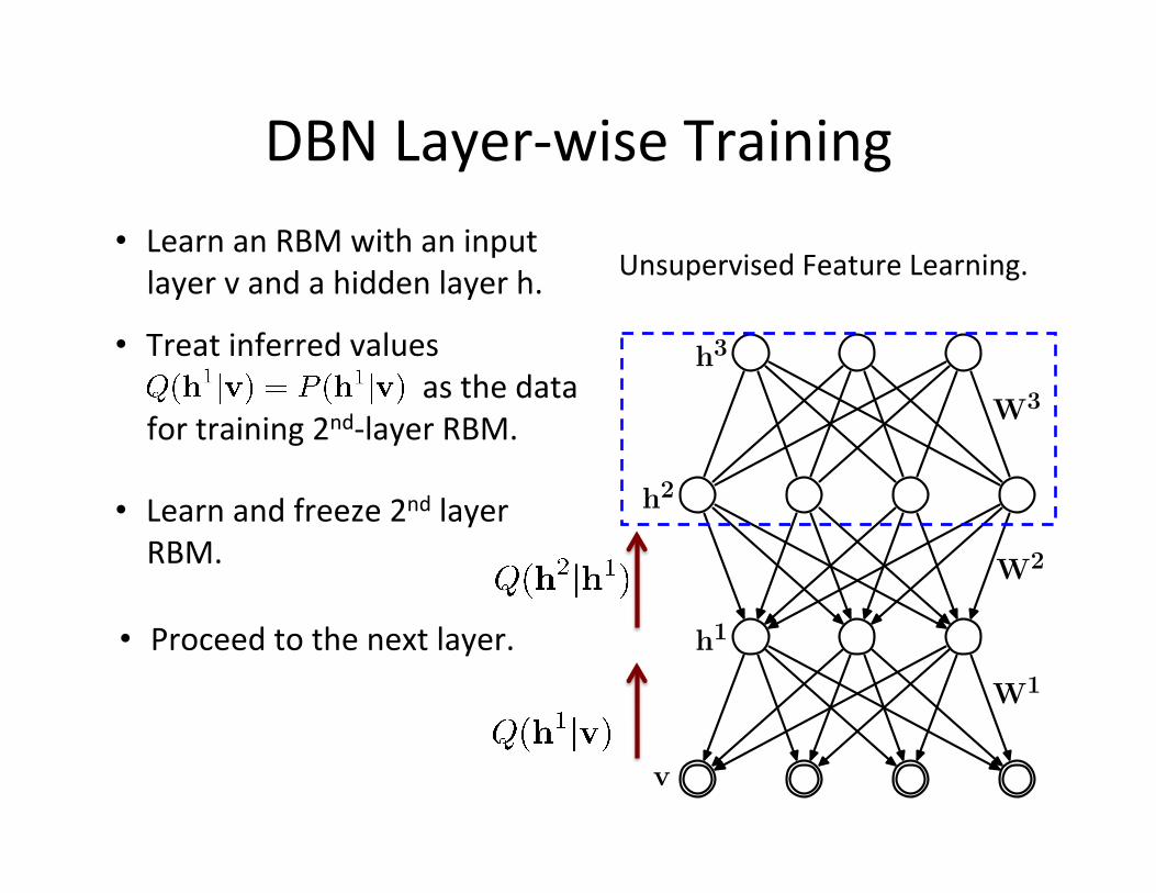
• Learn an RBM with an input layer v and a hidden layer h.
• Learn and freeze 2nd layer RBM.
• Treat inferred values as the data
for training 2nd-‐layer RBM.
Unsupervised Feature Learning.
DBN Layer-‐wise Training
v
h2
h1
h3
W1
W3
W2
• Proceed to the next layer.
• Learn an RBM with an input layer v and a hidden layer h.
• Learn and freeze 2nd layer RBM.
• Treat inferred values as the data
for training 2nd-‐layer RBM.
Unsupervised Feature Learning.
Layerwise pretraining improves varia=onal lower bound!
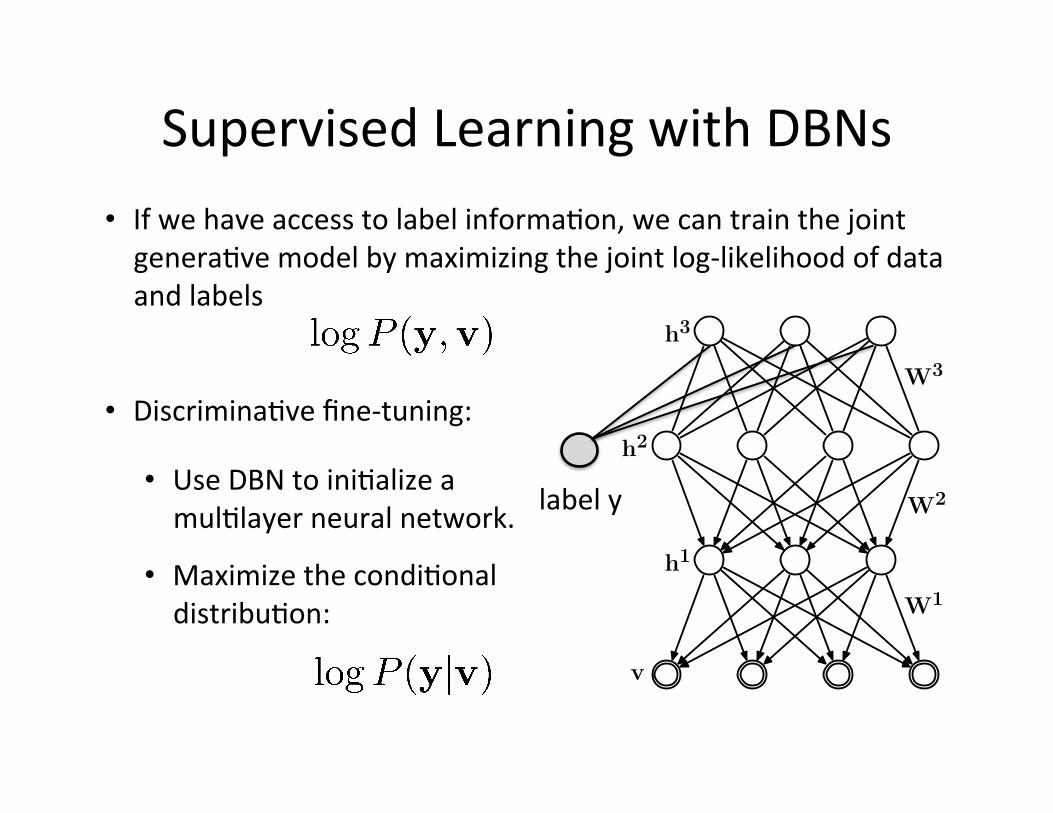
Supervised Learning with DBNs • If we have access to label informa=on, we can train the joint genera=ve model by maximizing the joint log-‐likelihood of data and labels
v
h2
h1
h3
W1
W3
W2label y
• Discrimina=ve fine-‐tuning:
• Use DBN to ini=alize a mul=layer neural network.
• Maximize the condi=onal distribu=on:
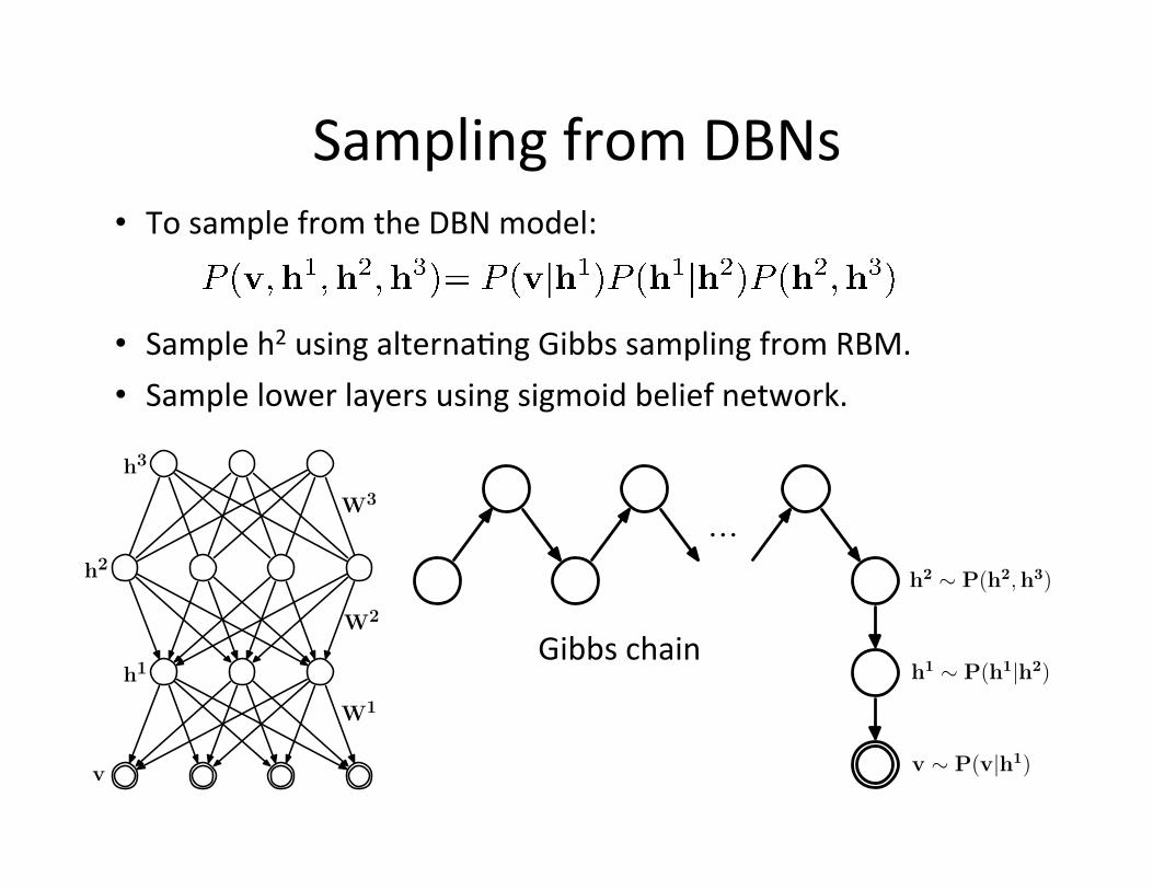
...h2 ∼ P(h2,h3)
h1 ∼ P(h1|h2)
v ∼ P(v|h1)
h3 ∼ Q(h3|h2)
h2 ∼ Q(h2|h1)
h1 ∼ Q(h1|v)
v
h3 ∼ Q̃(h3|v)
h2 ∼ Q̃(h2|v)
h1 ∼ Q̃(h1|v)
v
Sampling from DBNs • To sample from the DBN model:
• Sample h2 using alterna=ng Gibbs sampling from RBM. • Sample lower layers using sigmoid belief network.
v
h2
h1
h3
W1
W3
W2
Gibbs chain
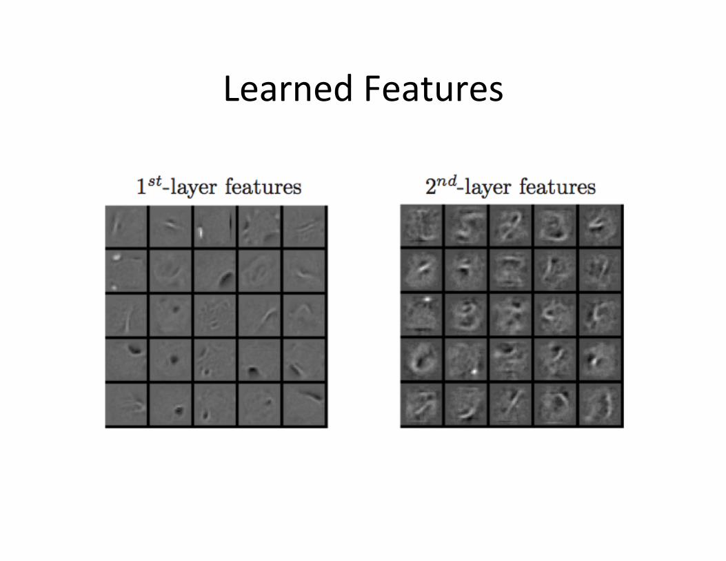
Learned Features
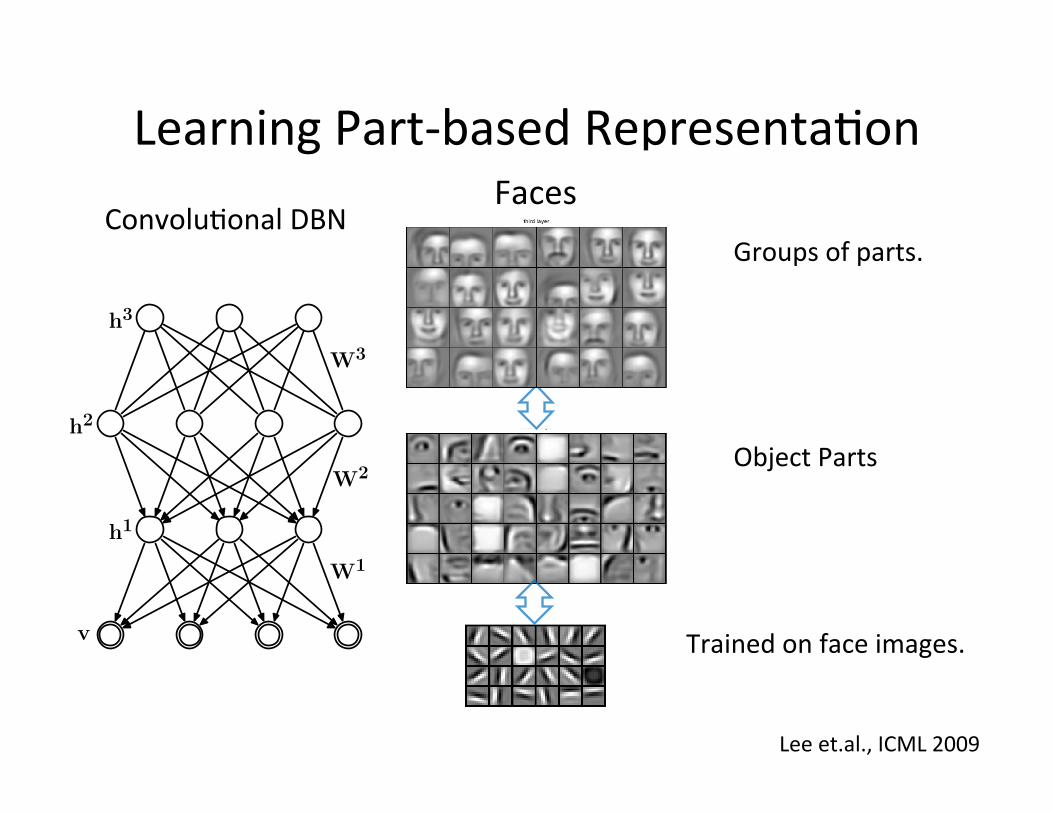
Learning Part-‐based Representa=on Convolu=onal DBN
Faces
v
h2
h1
h3
W1
W3
W2
Trained on face images.
Object Parts
Groups of parts.
Lee et.al., ICML 2009

Learning Part-‐based Representa=on Faces Cars Elephants Chairs
Lee et.al., ICML 2009
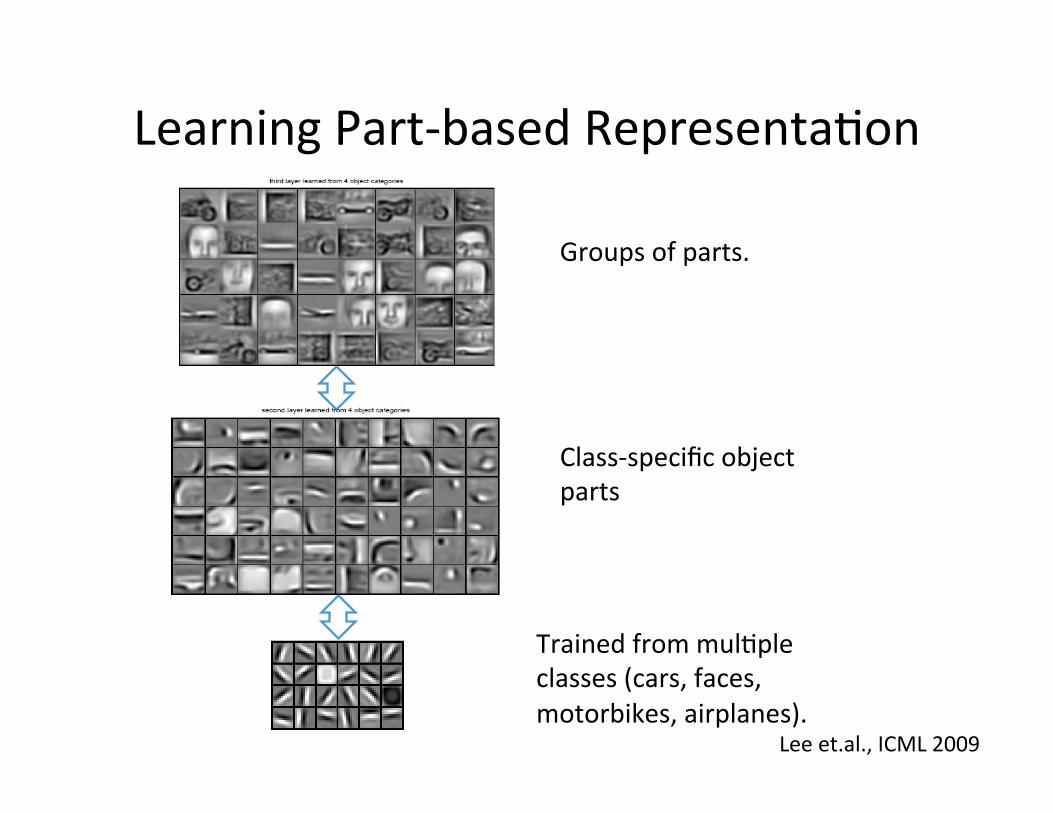
Learning Part-‐based Representa=on
Trained from mul=ple classes (cars, faces, motorbikes, airplanes).
Class-‐specific object parts
Groups of parts.
Lee et.al., ICML 2009
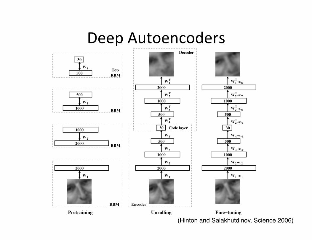
Deep Autoencoders
W
W
W +�
W
W
W
W
W +�
W +�
W +�
W
W +�
W +�
W +�
+�
W
W
W
W
W
W
1
2000
RBM
2
2000
1000
500
500
1000
1000
500
1 1
2000
2000
500500
1000
1000
2000
500
2000
T
4T
RBM
Pretraining Unrolling
1000 RBM
3
4
30
30
Fine�tuning
4 4
2 2
3 3
4T
5
3T
6
2T
7
1T
8
Encoder
1
2
3
30
4
3
2T
1T
Code layer
Decoder
RBMTop
(Hinton and Salakhutdinov, Science 2006)!

Deep Autoencoders • We used 25x25 – 2000 – 1000 – 500 – 30 autoencoder to extract 30-‐D real-‐valued codes for Olive� face patches.
• Top: Random samples from the test dataset. • Middle: Reconstruc=ons by the 30-‐dimensional deep autoencoder.
• BoTom: Reconstruc=ons by the 30-‐dimen=noal PCA.
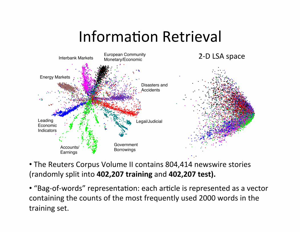
Informa=on Retrieval 2-‐D LSA space
Legal/JudicialLeading Economic Indicators
European Community Monetary/Economic
Accounts/Earnings
Interbank Markets
Government Borrowings
Disasters and Accidents
Energy Markets
• The Reuters Corpus Volume II contains 804,414 newswire stories (randomly split into 402,207 training and 402,207 test).
• “Bag-‐of-‐words” representa=on: each ar=cle is represented as a vector containing the counts of the most frequently used 2000 words in the training set.
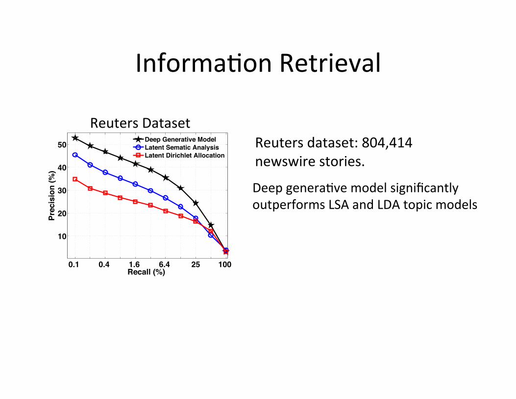
0.1 0.4 1.6 6.4 25 100
10
20
30
40
50
Recall (%)
Prec
isio
n (%
)
Deep Generative ModelLatent Sematic AnalysisLatent Dirichlet Allocation
Reuters Dataset
Deep genera=ve model significantly outperforms LSA and LDA topic models
Reuters dataset: 804,414 newswire stories.
Informa=on Retrieval
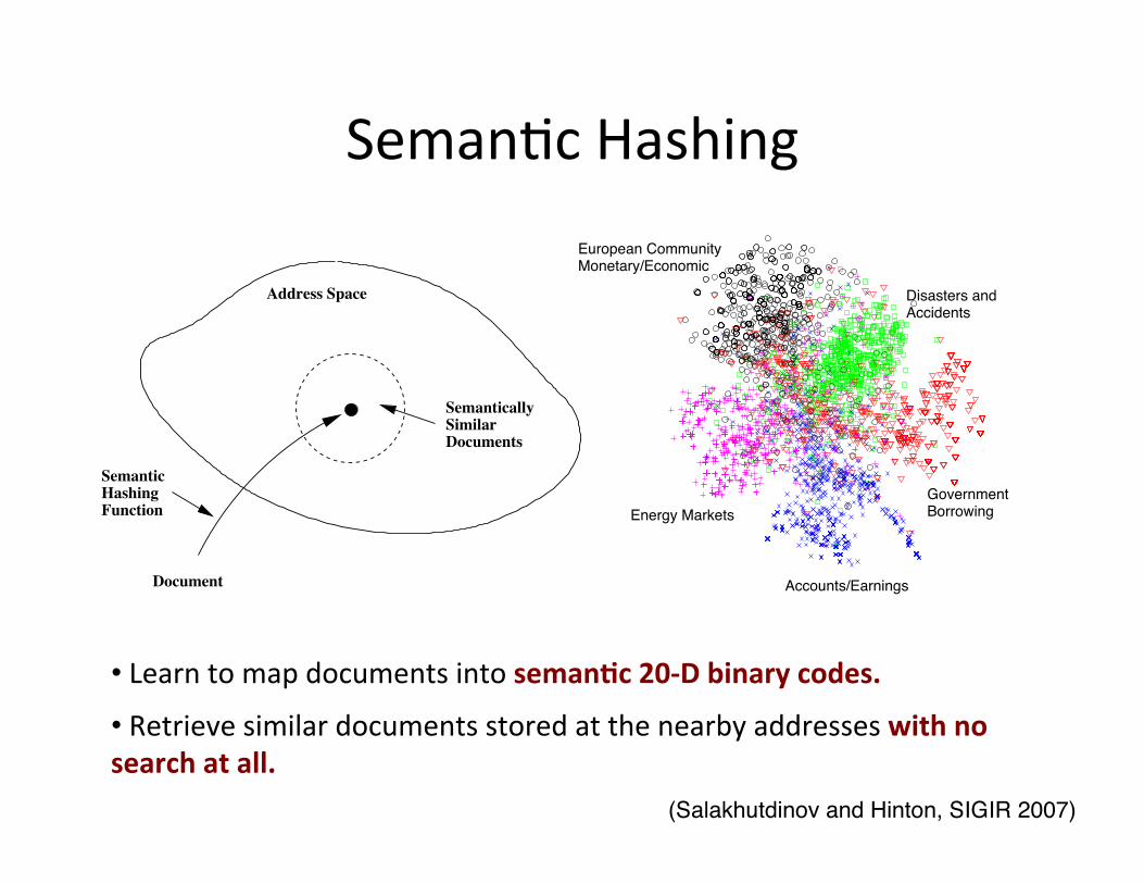
Seman=c Hashing
• Learn to map documents into semanWc 20-‐D binary codes.
• Retrieve similar documents stored at the nearby addresses with no search at all.
Accounts/Earnings
Government Borrowing
European Community Monetary/Economic
Disasters and Accidents
Energy Markets
SemanticallySimilarDocuments
Document
Address Space
SemanticHashingFunction
(Salakhutdinov and Hinton, SIGIR 2007)!
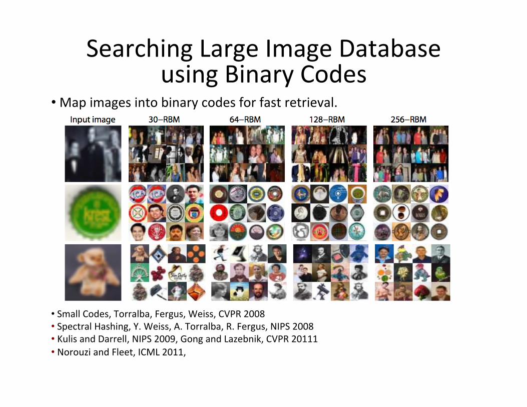
Searching Large Image Database using Binary Codes
• Map images into binary codes for fast retrieval.
• Small Codes, Torralba, Fergus, Weiss, CVPR 2008 • Spectral Hashing, Y. Weiss, A. Torralba, R. Fergus, NIPS 2008 • Kulis and Darrell, NIPS 2009, Gong and Lazebnik, CVPR 20111 • Norouzi and Fleet, ICML 2011,
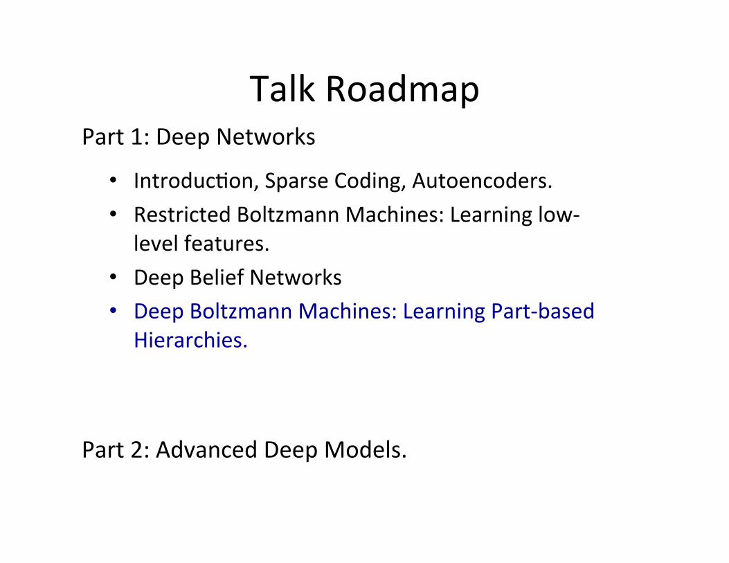
Talk Roadmap
• Introduc=on, Sparse Coding, Autoencoders. • Restricted Boltzmann Machines: Learning low-‐
level features. • Deep Belief Networks • Deep Boltzmann Machines: Learning Part-‐based
Hierarchies.
Part 1: Deep Networks
Part 2: Advanced Deep Models.
h3
h2
h1
v
W3
W2
W1
h3
h2
h1
v
W3
W2
W1
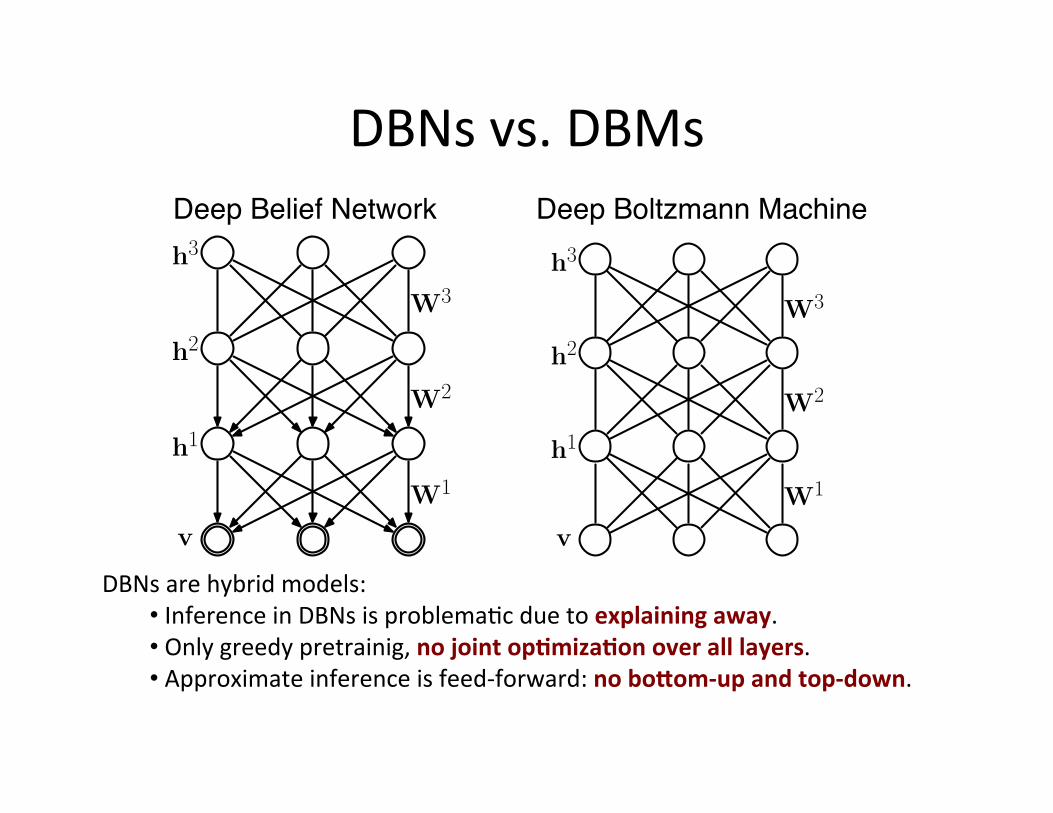
Deep Belief Network! Deep Boltzmann Machine!
DBNs vs. DBMs
DBNs are hybrid models: • Inference in DBNs is problema=c due to explaining away. • Only greedy pretrainig, no joint opWmizaWon over all layers. • Approximate inference is feed-‐forward: no boTom-‐up and top-‐down.
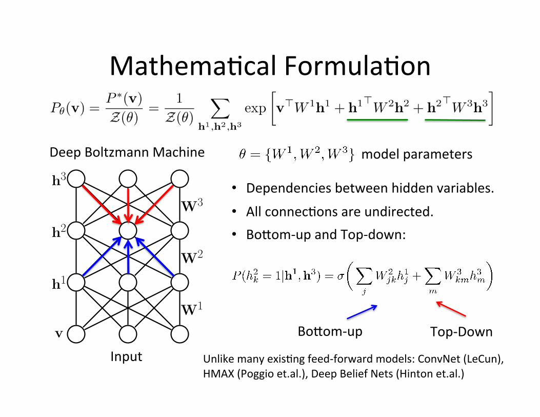
Mathema=cal Formula=on
h3
h2
h1
v
W3
W2
W1
model parameters
• Bo[om-‐up and Top-‐down:
Deep Boltzmann Machine
Bo[om-‐up Top-‐Down
Unlike many exis=ng feed-‐forward models: ConvNet (LeCun), HMAX (Poggio et.al.), Deep Belief Nets (Hinton et.al.)
• Dependencies between hidden variables. • All connec=ons are undirected.
Input
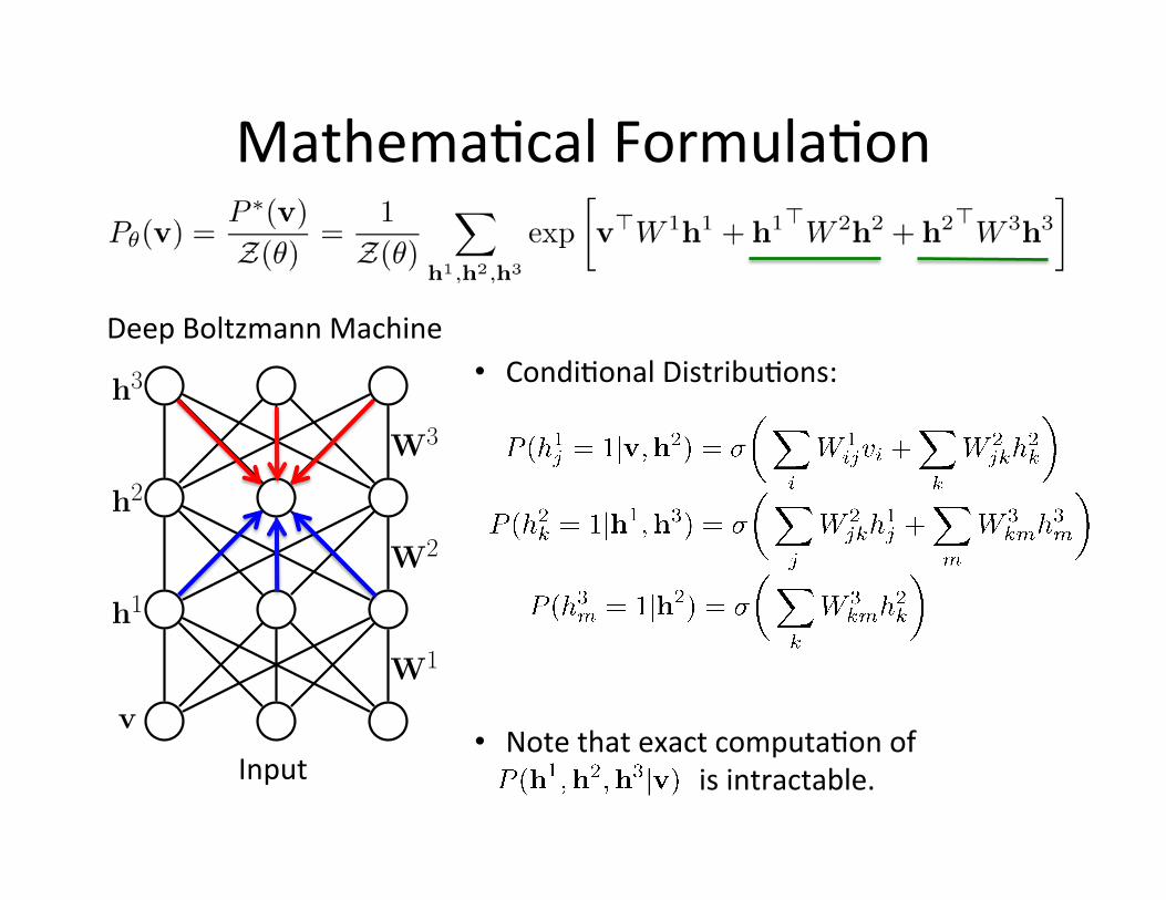
Mathema=cal Formula=on
h3
h2
h1
v
W3
W2
W1
Deep Boltzmann Machine • Condi=onal Distribu=ons:
Input • Note that exact computa=on of is intractable.

h3
h2
h1
v
W3
W2
W1
Neural Network Output
h3
h2
h1
v
W3
W2
W1
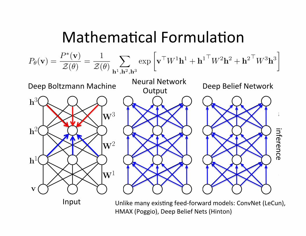
Mathema=cal Formula=on
Deep Boltzmann Machine
h3
h2
h1
v
W3
W2
W1
Deep Belief Network
Unlike many exis=ng feed-‐forward models: ConvNet (LeCun), HMAX (Poggio), Deep Belief Nets (Hinton)
Input
h3
h2
h1
v
W3
W2
W1
h3
h2
h1
v
W3
W2
W1
Mathema=cal Formula=on
Deep Boltzmann Machine Deep Belief Network
h3
h2
h1
v
W3
W2
W1
Unlike many exis=ng feed-‐forward models: ConvNet (LeCun), HMAX (Poggio), Deep Belief Nets (Hinton)
inference
Neural Network Output
Input
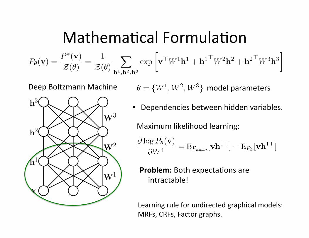
Mathema=cal Formula=on
model parameters
Maximum likelihood learning:
Problem: Both expecta=ons are intractable!
Learning rule for undirected graphical models: MRFs, CRFs, Factor graphs.
• Dependencies between hidden variables.
Deep Boltzmann Machine
h3
h2
h1
v
W3
W2
W1
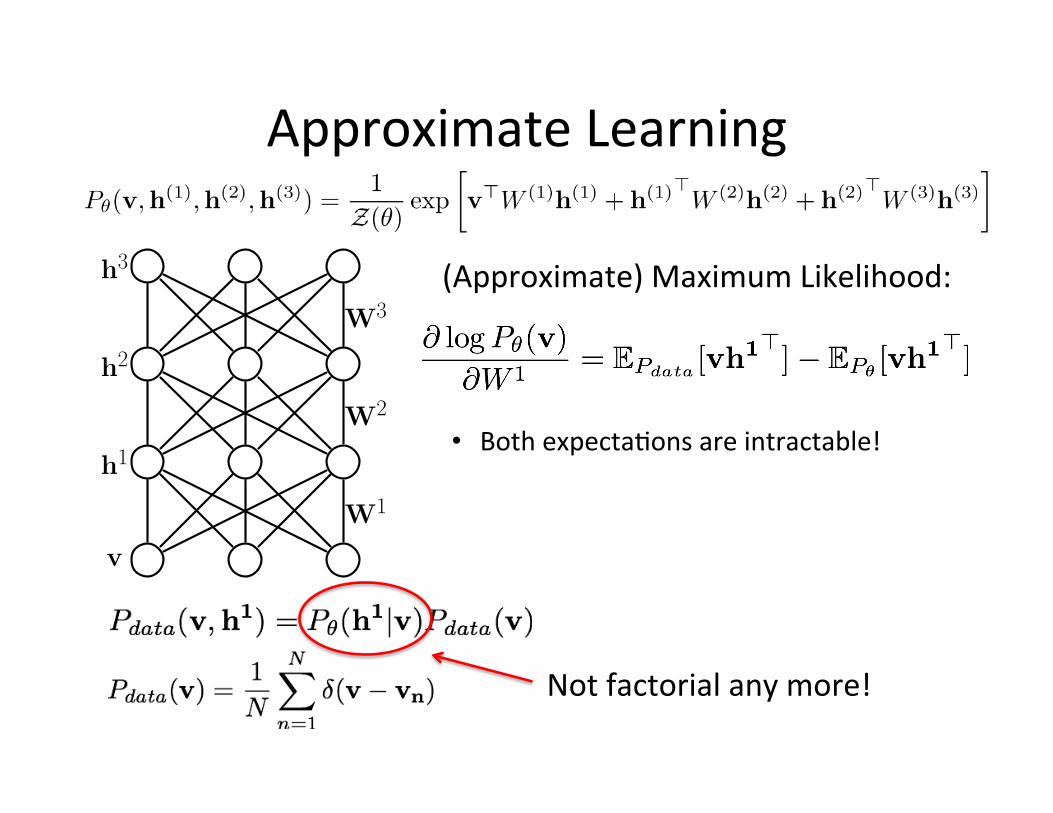
Approximate Learning
(Approximate) Maximum Likelihood:
Not factorial any more!
h3
h2
h1
v
W3
W2
W1
• Both expecta=ons are intractable!

Data
Approximate Learning
(Approximate) Maximum Likelihood: h3
h2
h1
v
W3
W2
W1
Not factorial any more!
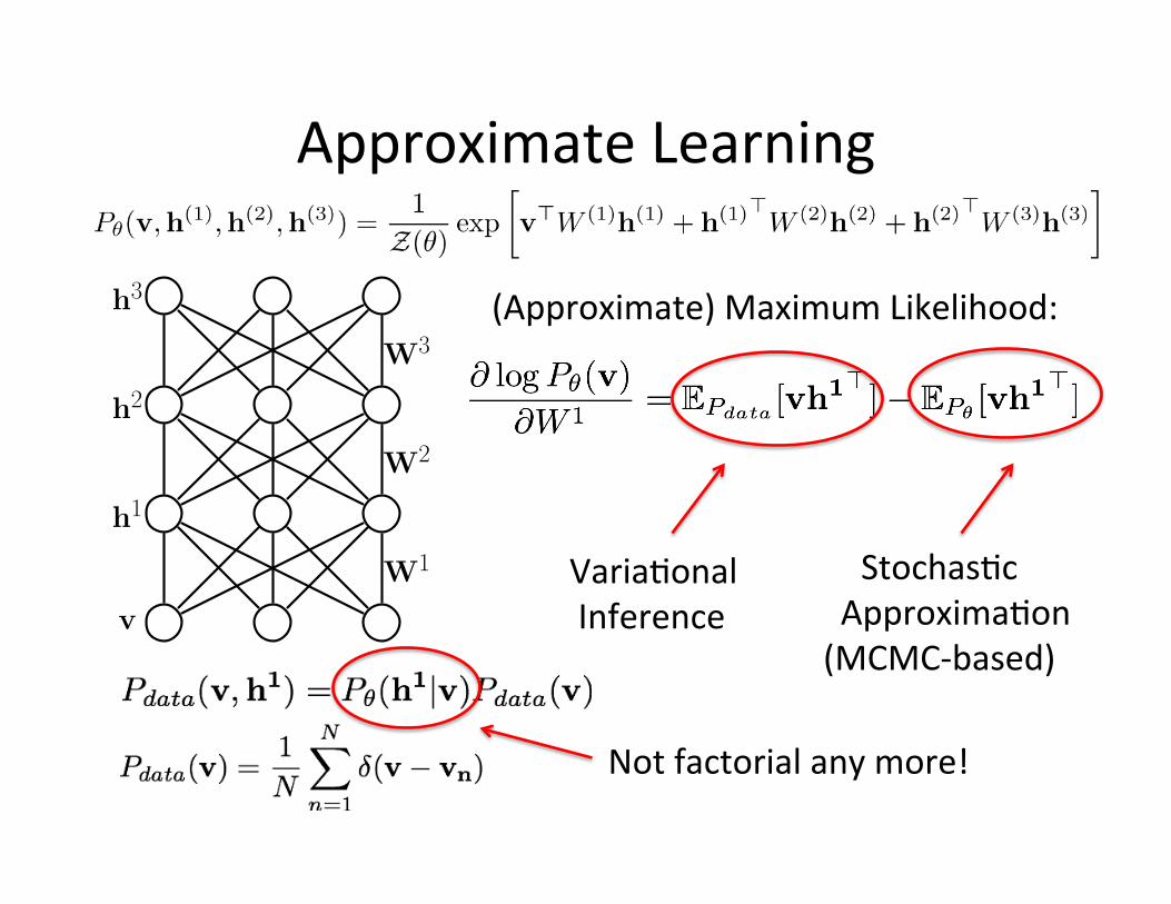
Approximate Learning
(Approximate) Maximum Likelihood:
Not factorial any more!
h3
h2
h1
v
W3
W2
W1 Varia=onal Inference
Stochas=c Approxima=on (MCMC-‐based)
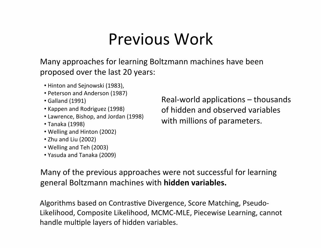
Previous Work Many approaches for learning Boltzmann machines have been proposed over the last 20 years:
• Hinton and Sejnowski (1983), • Peterson and Anderson (1987) • Galland (1991) • Kappen and Rodriguez (1998) • Lawrence, Bishop, and Jordan (1998) • Tanaka (1998) • Welling and Hinton (2002) • Zhu and Liu (2002) • Welling and Teh (2003) • Yasuda and Tanaka (2009)
Many of the previous approaches were not successful for learning general Boltzmann machines with hidden variables.
Real-‐world applica=ons – thousands of hidden and observed variables with millions of parameters.
Algorithms based on Contras=ve Divergence, Score Matching, Pseudo-‐Likelihood, Composite Likelihood, MCMC-‐MLE, Piecewise Learning, cannot handle mul=ple layers of hidden variables.
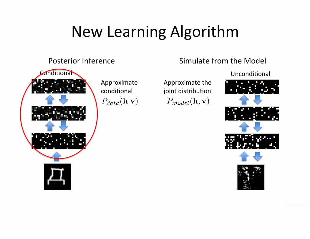
New Learning Algorithm
Condi=onal Uncondi=onal
Posterior Inference Simulate from the Model
Approximate condi=onal
Approximate the joint distribu=on
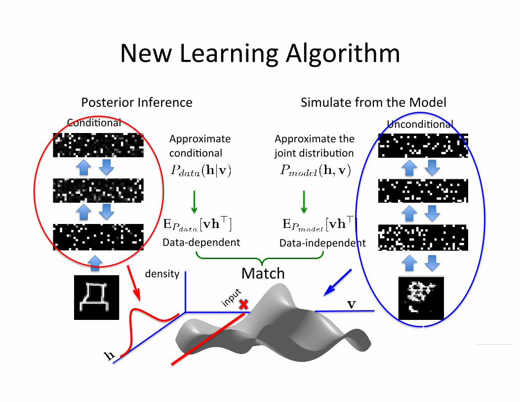
Condi=onal Uncondi=onal
Posterior Inference Simulate from the Model
Approximate the joint distribu=on
Data-‐dependent
Approximate condi=onal
New Learning Algorithm
Data-‐independent
density Match
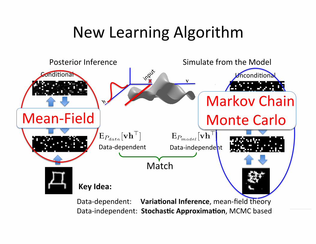
Condi=onal Uncondi=onal
Posterior Inference Simulate from the Model
Approximate the joint distribu=on
Data-‐dependent
Approximate condi=onal
New Learning Algorithm
Data-‐independent
Match
Key Idea:
Markov Chain Monte Carlo
Data-‐dependent: VariaWonal Inference, mean-‐field theory Data-‐independent: StochasWc ApproximaWon, MCMC based
Mean-‐Field
h2
h1
v
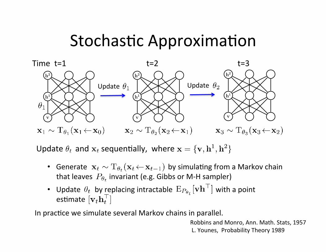
Time t=1
Stochas=c Approxima=on
Update Update h2
h1
v
t=2 h2
h1
v
t=3
• Generate by simula=ng from a Markov chain that leaves invariant (e.g. Gibbs or M-‐H sampler)
• Update by replacing intractable with a point es=mate
In prac=ce we simulate several Markov chains in parallel. Robbins and Monro, Ann. Math. Stats, 1957 L. Younes, Probability Theory 1989
Update and sequen=ally, where
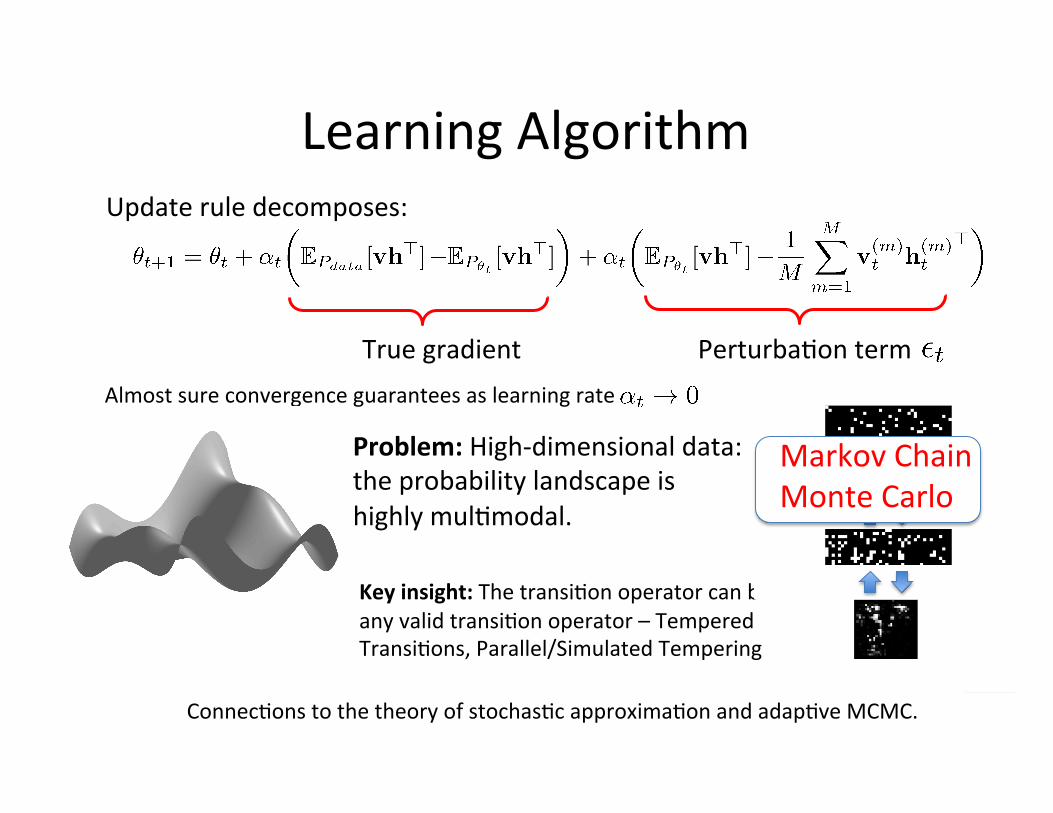
Learning Algorithm Update rule decomposes:
True gradient Perturba=on term Almost sure convergence guarantees as learning rate
Problem: High-‐dimensional data: the probability landscape is highly mul=modal.
Connec=ons to the theory of stochas=c approxima=on and adap=ve MCMC.
Key insight: The transi=on operator can be any valid transi=on operator – Tempered Transi=ons, Parallel/Simulated Tempering.
Markov Chain Monte Carlo
Posterior Inference
Mean-‐Field
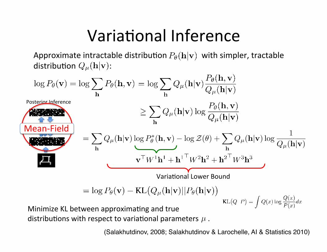
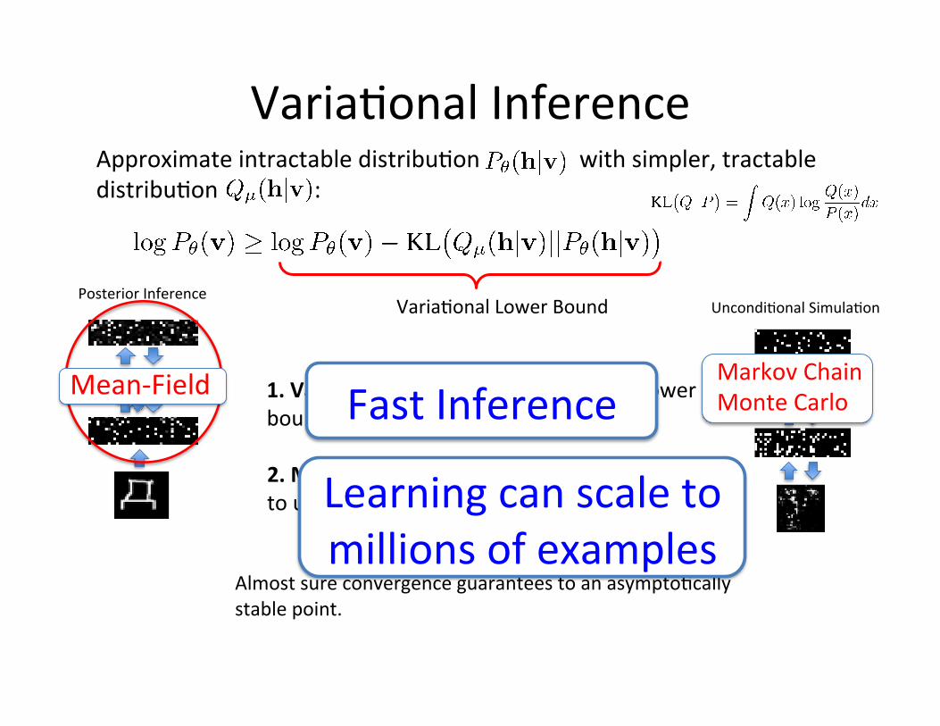
Varia=onal Inference Approximate intractable distribu=on with simpler, tractable distribu=on :
(Salakhutdinov, 2008; Salakhutdinov & Larochelle, AI & Statistics 2010)!
Varia=onal Lower Bound
Minimize KL between approxima=ng and true distribu=ons with respect to varia=onal parameters .
Posterior Inference
Mean-‐Field
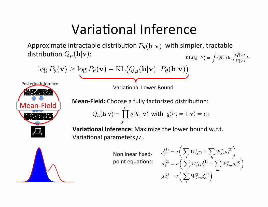
Varia=onal Inference Approximate intractable distribu=on with simpler, tractable distribu=on :
Mean-‐Field: Choose a fully factorized distribu=on:
with
Nonlinear fixed-‐ point equa=ons:
VariaWonal Inference: Maximize the lower bound w.r.t. Varia=onal parameters .
Varia=onal Lower Bound
Posterior Inference
Mean-‐Field
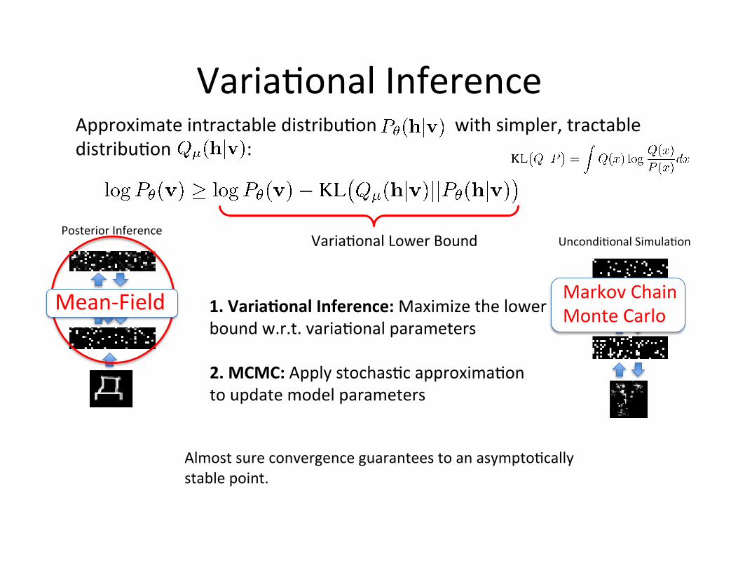
Varia=onal Inference Approximate intractable distribu=on with simpler, tractable distribu=on :
1. VariaWonal Inference: Maximize the lower bound w.r.t. varia=onal parameters
Markov Chain Monte Carlo
2. MCMC: Apply stochas=c approxima=on to update model parameters
Almost sure convergence guarantees to an asympto=cally stable point.
Uncondi=onal Simula=on Varia=onal Lower Bound
Posterior Inference
Mean-‐Field
Varia=onal Inference Approximate intractable distribu=on with simpler, tractable distribu=on :
1. VariaWonal Inference: Maximize the lower bound w.r.t. varia=onal parameters
Markov Chain Monte Carlo
2. MCMC: Apply stochas=c approxima=on to update model parameters
Almost sure convergence guarantees to an asympto=cally stable point.
Uncondi=onal Simula=on
Fast Inference
Learning can scale to millions of examples
Varia=onal Lower Bound
Good Genera=ve Model? Handwri[en Characters

Good Genera=ve Model? Handwri[en Characters
Good Genera=ve Model? Handwri[en Characters
Real Data Simulated

Good Genera=ve Model? Handwri[en Characters
Real Data Simulated
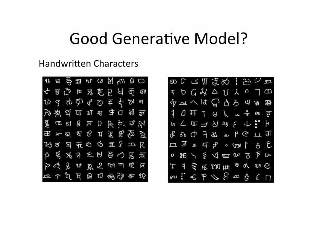
Good Genera=ve Model? Handwri[en Characters
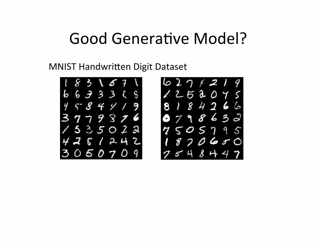
Good Genera=ve Model? MNIST Handwri[en Digit Dataset
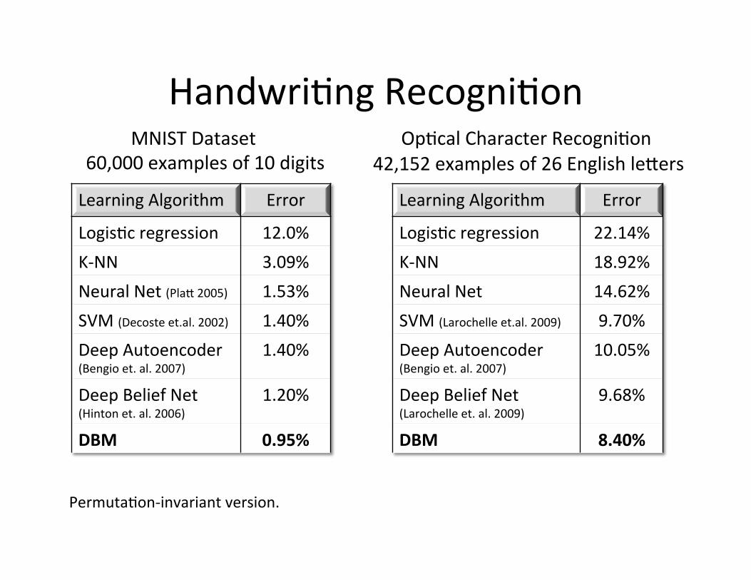
Handwri=ng Recogni=on
Learning Algorithm Error
Logis=c regression 12.0% K-‐NN 3.09% Neural Net (Pla[ 2005) 1.53% SVM (Decoste et.al. 2002) 1.40% Deep Autoencoder (Bengio et. al. 2007)
1.40%
Deep Belief Net (Hinton et. al. 2006)
1.20%
DBM 0.95%
Learning Algorithm Error
Logis=c regression 22.14% K-‐NN 18.92% Neural Net 14.62% SVM (Larochelle et.al. 2009) 9.70% Deep Autoencoder (Bengio et. al. 2007)
10.05%
Deep Belief Net (Larochelle et. al. 2009)
9.68%
DBM 8.40%
MNIST Dataset Op=cal Character Recogni=on 60,000 examples of 10 digits 42,152 examples of 26 English le[ers
Permuta=on-‐invariant version.
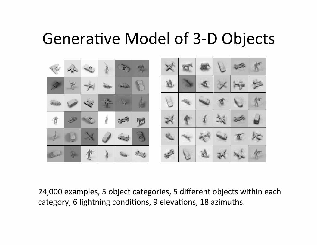
Genera=ve Model of 3-‐D Objects
24,000 examples, 5 object categories, 5 different objects within each category, 6 lightning condi=ons, 9 eleva=ons, 18 azimuths.

3-‐D Object Recogni=on
Learning Algorithm Error Logis=c regression 22.5% K-‐NN (LeCun 2004) 18.92% SVM (Bengio & LeCun 2007) 11.6% Deep Belief Net (Nair & Hinton 2009)
9.0%
DBM 7.2%
Pa[ern Comple=on
Permuta=on-‐invariant version.
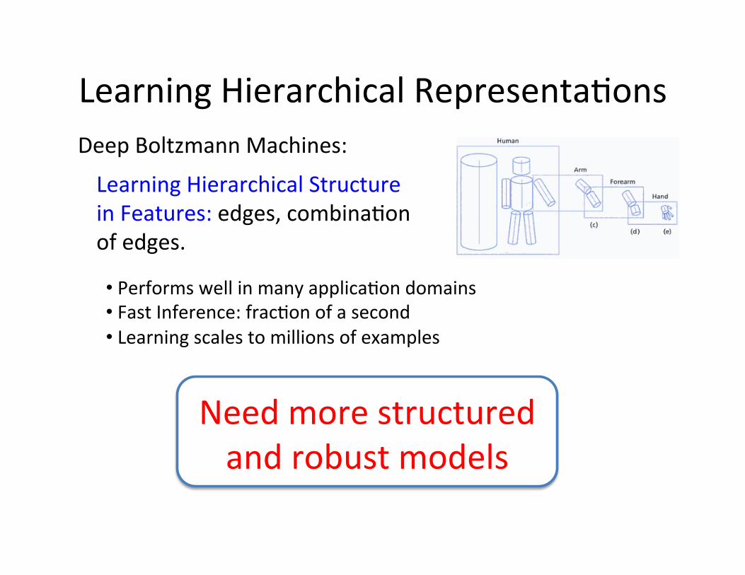
Learning Hierarchical Representa=ons Deep Boltzmann Machines:
Learning Hierarchical Structure in Features: edges, combina=on of edges.
• Performs well in many applica=on domains • Fast Inference: frac=on of a second • Learning scales to millions of examples
Need more structured and robust models
Second Part of Tutorial
• Learning structured and Robust Models • One-‐Shot Learning • Transfer Learning • Applica=ons in vision and NLP
Part 1: Advanced Deep Learning Models
Part 2: Mul=modal Deep Learning
• Mul=modal DBMs for images and text • Cap=on Genera=on with Recurrent RNNs • Skip-‐Thought vectors for NLP

End of Part 1