Learning Deep Generative Models

9.520 Class 19

Ruslan SalakhutdinovBCS and CSAIL, MIT

1

Talk Outline

1. Introduction.

1. Autoencoders, Boltzmann Machines.

2. Deep Belief Networks (DBN’s).

3. Learning Feature Hierarchies with DBN’s.

4. Deep Boltzmann Machines (DBM’s).

5. Extensions.

2

Long-term Goal

Raw pixel values

Slightly higher level representation

...

High level representationTiger rests on the grass

Learn progressively complex high-

level representations.

Use bottom-up + top-down cues.

Build high-level representations

from large unlabeled datasets.

Labeled data is used to only slightly

adjust the model for a specific task.

3

Challenges

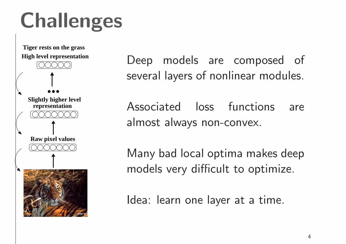
Raw pixel values

Slightly higher level representation

...

High level representationTiger rests on the grass

Deep models are composed of

several layers of nonlinear modules.

Associated loss functions are

almost always non-convex.

Many bad local optima makes deep

models very difficult to optimize.

Idea: learn one layer at a time.

4

Key Requirements

Raw pixel values

Slightly higher level representation

...

High level representationTiger rests on the grass

Online Learning.

Learning should scale to large

datasets, containing millions or

billions examples.

Inferring high-level representation

should be fast: fraction of a

second.

Demo.

5

AutoencodersDecoder

v

h

v

Code Layer

Encoder

W

W

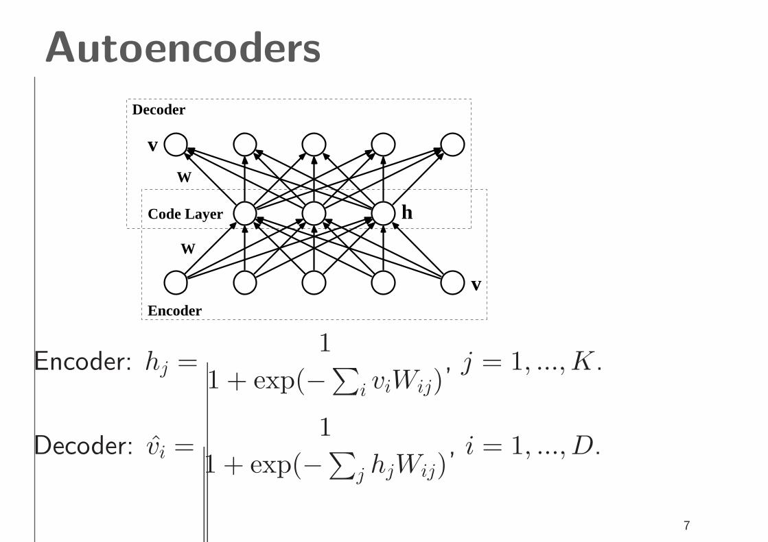
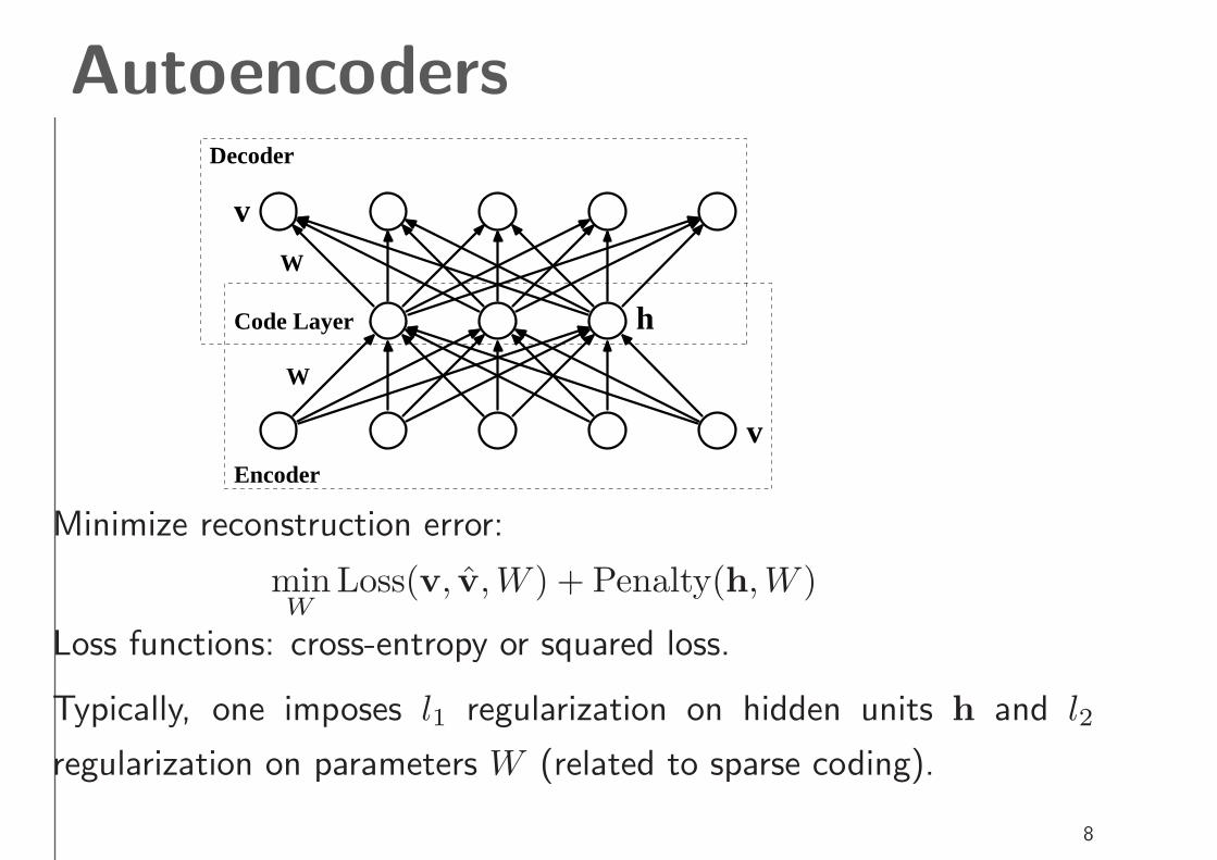
Consider having D binary visible units v and K binary

hidden units h.

Idea: transform data into a (low-dimensional) code and

then reconstruct the data from the code.

6

AutoencodersDecoder

v

h

v

Code Layer

Encoder

W

W

Encoder: hj =1

1 + exp(−∑

i viWij), j = 1, ...,K.

Decoder: v̂i =1

1 + exp(−∑

j hjWij), i = 1, ...,D.

7

AutoencodersDecoder

v

h

v

Code Layer

Encoder

W

W

Minimize reconstruction error:

minW

Loss(v, v̂,W ) + Penalty(h,W )

Loss functions: cross-entropy or squared loss.

Typically, one imposes l1 regularization on hidden units h and l2

regularization on parameters W (related to sparse coding).

8

Building Block: RBM’sProbabilistic Analog: Restricted Boltzmann Machines.

h

v

W

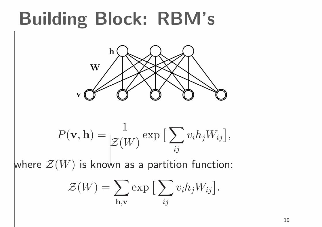
Visible stochastic binary units v are connected to hidden

stochastic binary feature detectors h:

P (v,h) =1

Z(W )exp

[

∑

ij

vihjWij

]

Markov Random Fields, Log-linear Models, Boltzmann machines.

9

Building Block: RBM’s

h

v

W

P (v,h) =1

Z(W )exp

[

∑

ij

vihjWij

]

,

where Z(W ) is known as a partition function:

Z(W ) =∑

h,v

exp[

∑

ij

vihjWij

]

.

10

Inference with RBM’s

P (v,h) =1

Zexp

(

∑

ij

vihjWij

)

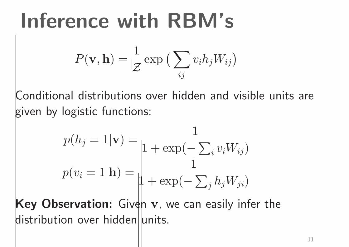
Conditional distributions over hidden and visible units are

given by logistic functions:

p(hj = 1|v) =1

1 + exp(−∑

i viWij)

p(vi = 1|h) =1

1 + exp(−∑

j hjWji)

Key Observation: Given v, we can easily infer the

distribution over hidden units.

11

Learning with RBM’s

Pmodel(v) =∑

h

P (v,h) =1

Z

∑

h

exp(

∑

ij

vihjWij

)

Maximum Likelihood learning:

∂ log P (v)

∂Wij

= EPdata[vihj] − EPmodel

[vihj],

where Pdata(h,v) = P (h|v)Pdata(v), with

Pdata(v) representing the empirical distribution.

However, computing EPmodelis difficult due to the presence

of a partition function Z.

12

Contrastive Divergence

i i

j

i

j

data1

<v h >i

j

j <v h >i j <v h >i j inf

data reconstruction fantasy

Maximum Likelihood learning:

∆Wij = EPdata[vihj] − EPmodel

[vihj]

Contrastive Divergence learning:

∆Wij = EPdata[vihj] − EPT

[vihj]

PT represents a distribution defined by running a Gibbs chain,

initialized at the data, for T full steps.

13

Learning with RBM’s

MNIST Digits NORB 3D Objects

Learned W

14

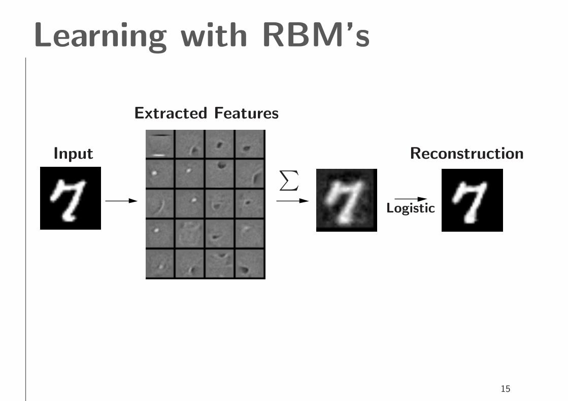
Learning with RBM’s

Input

Extracted Features

∑

Logistic

Reconstruction

15

Modeling DocumentsRestricted Boltzmann Machines: 2-layer modules.

h

v

W

• Visible units are multinomials over word counts.

• Hidden units are topic detectors.

16

Extracted Latent Topics20 Newsgroup 2−D Topic Space

comp.graphics

rec.sport.hockey

sci.cryptography

soc.religion.christian

talk.politics.guns

talk.politics.mideast

17

Collaborative FilteringForm of Matrix Factorization.

h

v

W

• Visible units are multinomials over rating values.

• Hidden units are user preference detectors.

Used in Netflix competition.

18

Deep Belief Networks (DBN’s)• There are limitations on the types of structure that can

be represented efficiently by a single layer of hidden

variables.

• We would like to efficiently learn multi-layer models

using a large supply of high-dimensional highly-

structured unlabeled sensory input.

19

Learning DBN’s

RBM

RBM

RBM

Greedy, layer-by-layer learning:

• Learn and Freeze W 1.

• Sample h1 ∼ P (h1|v;W 1).

Treat h1 as if it were data.

• Learn and Freeze W 2.

• ...

Learn high-level representations.

20

Learning DBN’s

RBM

RBM

RBM

Under certain conditions adding

an extra layer always improves

a lower bound on the log probability

of data.

Each layer of features captures

high-order correlations between

the activities of units in the

layer below.

21

Learning DBN’s

1st-layer features 2nd-layer features

22

Density Estimation

DBN samples Mixture of Bernoulli’s

MoB, test log-prob: -137.64 per digit.

DBN, test log-prob: -85.97 per digit.

Difference of over 50 nats is quite large.

23

Learning Deep Autoencoders

W

W

W

W

1

2000

RBM

2

2000

1000

500

RBM500

RBM

1000 RBM

3

4

30

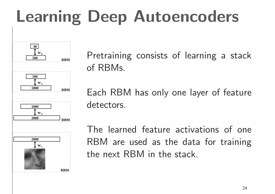
Pretraining consists of learning a stack

of RBMs.

Each RBM has only one layer of feature

detectors.

The learned feature activations of one

RBM are used as the data for training

the next RBM in the stack.

24

Learning Deep Autoencoders

W

W

W

W

W

W

W

W

500

1000

2000

500

2000

Unrolling

Encoder

1

2

3

30

4

3

2

1

Code layer

Decoder

4

1000

T

T

T

T

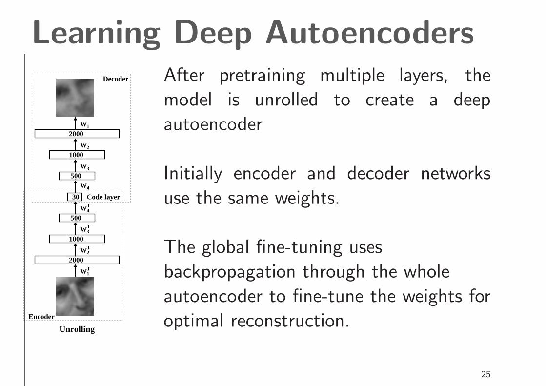
After pretraining multiple layers, the

model is unrolled to create a deep

autoencoder

Initially encoder and decoder networks

use the same weights.

The global fine-tuning uses

backpropagation through the whole

autoencoder to fine-tune the weights for

optimal reconstruction.

25

Learning Deep Autoencoders

W

W

W +ε

W

W

W

W

W +ε

W +ε

W +ε

W

W +ε

W +ε

W +ε

+ε

W

W

W

W

W

W

1

2000

RBM

2

2000

1000

500

500

1000

1000

500

1 1

2000

2000

500500

1000

1000

2000

500

2000

T

4T

RBM

Pretraining Unrolling

1000 RBM

3

4

30

30

Fine−tuning

4 4

2 2

3 3

4T

5

3T

6

2T

7

1T

8

Encoder

1

2

3

30

4

3

2T

1T

Code layer

Decoder

RBMTop

26

Learning Deep AutoencodersWe used a 25 × 25-2000-1000-500-30 autoencoder to extract 30-D

real-valued codes for Olivetti face patches (7 hidden layers is usually

hard to train).

Top Random samples from the test dataset; Middle reconstructions

by the 30-dimensional deep autoencoder; and Bottom reconstructions

by 30-dimensional PCA.

27

Dimensionality Reduction

Legal/JudicialLeading Economic Indicators

European Community Monetary/Economic

Accounts/Earnings

Interbank Markets

Government Borrowings

Disasters and Accidents

Energy Markets

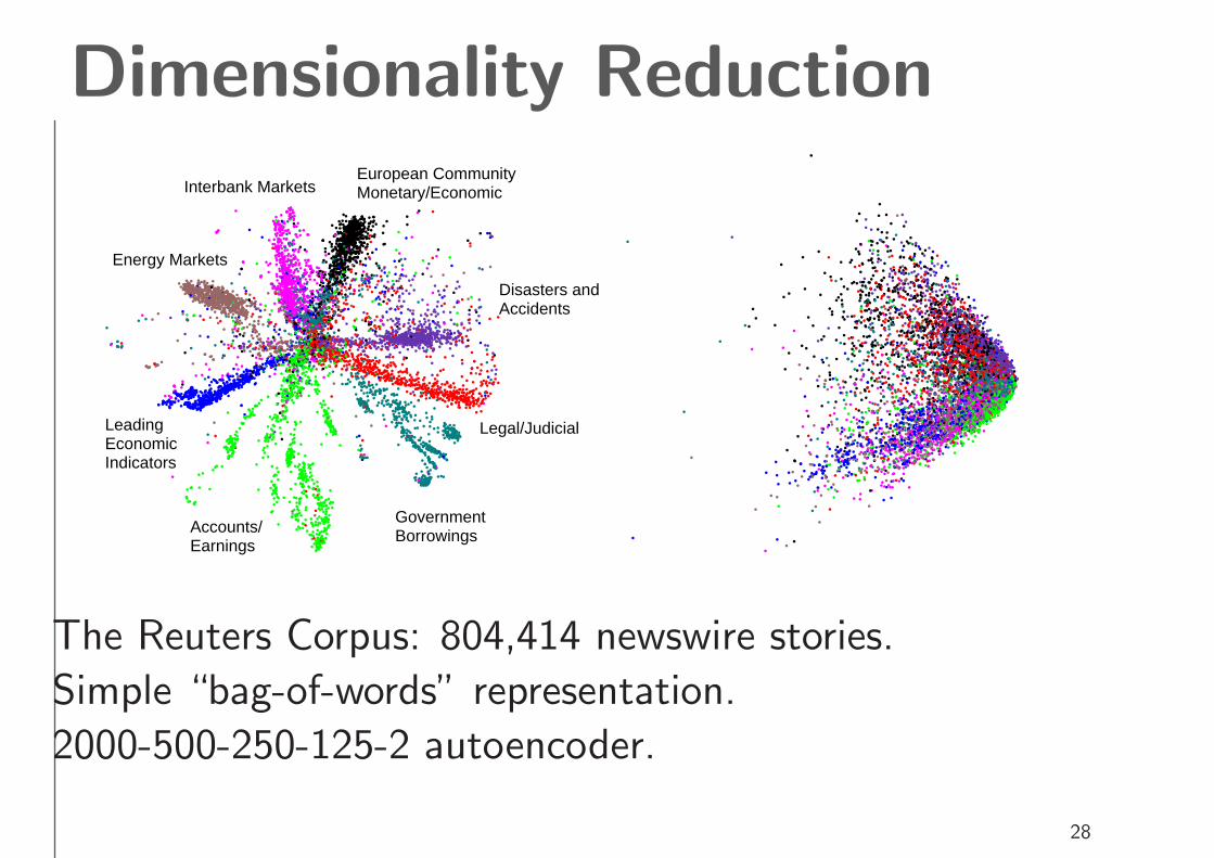
The Reuters Corpus: 804,414 newswire stories.

Simple “bag-of-words” representation.

2000-500-250-125-2 autoencoder.

28

Document Retrieval

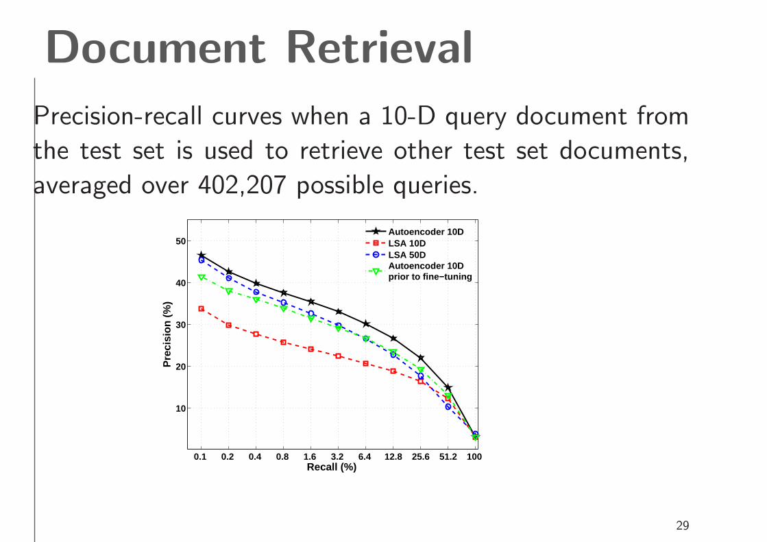
Precision-recall curves when a 10-D query document from

the test set is used to retrieve other test set documents,

averaged over 402,207 possible queries.

0.1 0.2 0.4 0.8 1.6 3.2 6.4 12.8 25.6 51.2 100

10

20

30

40

50

Recall (%)

Pre

cisi

on (

%)

Autoencoder 10DLSA 10DLSA 50DAutoencoder 10Dprior to fine−tuning

29

Semi-supervised Learning• Given a set of i.i.d labeled training samples {xl, yl}.

• Discriminative models model p(yl|xl; θ) directly (logistic

regression, Gaussian process, SVM’s).

• For many applications we have a large supply of high-

dimensional unlabeled data {xu}.

• Need to make some assumptions about the input

data {xu}.

• Otherwise unlabeled data is of no use.

30

Semi-supervised Learning

Key points of learning deep generative models:

• Learn probabilistic model p(xu; θ).

• Use learned parameters to initialize a discriminative

model p(yl|xl; θ) (neural network).

• Slightly adjust discriminative model for a specific task.

No knowledge of subsequent discriminative task during unsupervised

learning. Most of the information in parameters comes from learning

a generative model.

31

Classification Task

W +εW

W

W

W +ε

W +ε

W +ε

W

W

W

W

1 11

500 500

500

2000

500

500

2000

5002

500

RBM

500

2000

3

Pretraining Unrolling Fine−tuning

4 4

2 2

3 3

1

2

3

4

RBM

10

Softmax Output

10RBM

T

T

T

T

T

T

T

T

Classification error is 1.2% on MNIST, SVM’s get 1.4% and randomly

initialized backprop gets 1.6%.

Pretraining helps generalization – most of the information in theweights comes from modeling the input data. (Code available online)

32

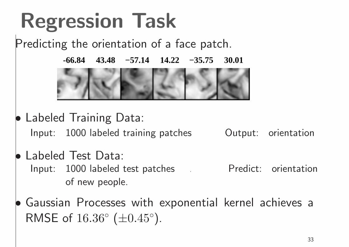
Regression TaskPredicting the orientation of a face patch.

-66.84 43.48 14.22 30.01−57.14 −35.75

• Labeled Training Data:Input: 1000 labeled training patches Output: orientation

• Labeled Test Data:Input: 1000 labeled test patches . Predict: orientation

of new people.

• Gaussian Processes with exponential kernel achieves a

RMSE of 16.36◦ (±0.45◦).

33

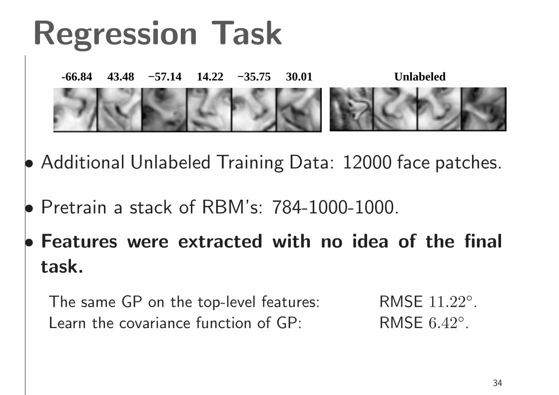
Regression Task-66.84 43.48 14.22 30.01−57.14 −35.75 Unlabeled

• Additional Unlabeled Training Data: 12000 face patches.

• Pretrain a stack of RBM’s: 784-1000-1000.

• Features were extracted with no idea of the final

task.

The same GP on the top-level features: RMSE 11.22◦.

Learn the covariance function of GP: RMSE 6.42◦.

34

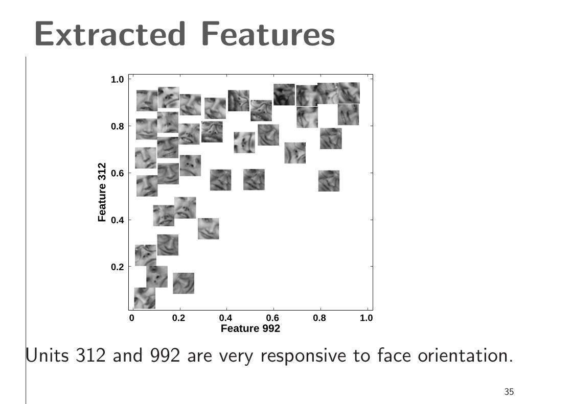
Extracted Features

Feature 992

Fea

ture

312

0 0.2 0.4 0.6 0.8 1.0

1.0

0.8

0.6

0.4

0.2

Units 312 and 992 are very responsive to face orientation.

35

DBM’s vs. DBN’s

h3

h2

h1

v

W3

W2

W1

h3

h2

h1

v

W3

W2

W1

Deep Boltzmann Machine Deep Belief Network

36

Deep Boltzmann Machines• DBM is a type of Markov random field, where all connections

between layers are undirected.

• DBM’s have the potential of learning internal representations that

become increasingly complex at higher layers, which is a promising

way of solving object and speech recognition problems.

• The approximate inference procedure, in addition to a bottom-up

pass, can incorporate top-down feedback, allowing DBM’s to better

propagate uncertainty about ambiguous inputs.

• The entire model can be trained online, processing one example at

a time.

37

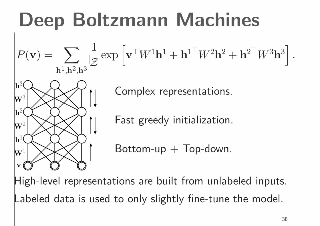
Deep Boltzmann Machines

P (v) =∑

h1,h2,h3

1

Zexp

[

v⊤W 1

h1 + h

1⊤W 2h

2 + h2⊤W 3

h3]

.

h3

h2

h1

v

W3

W2

W1

Complex representations.

Fast greedy initialization.

Bottom-up + Top-down.

High-level representations are built from unlabeled inputs.

Labeled data is used to only slightly fine-tune the model.

38

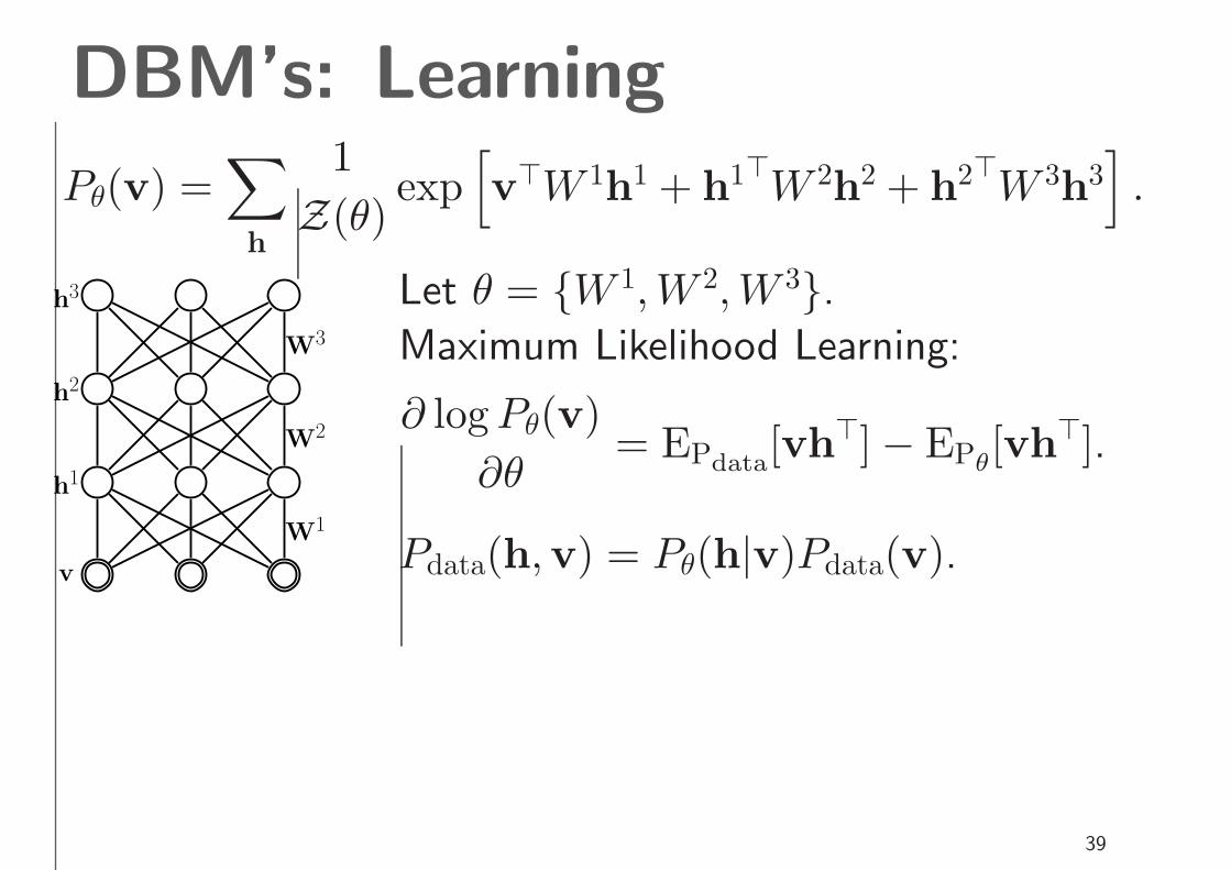
DBM’s: Learning

Pθ(v) =∑

h

1

Z(θ)exp

[

v⊤W 1

h1 + h

1⊤W 2h

2 + h2⊤W 3

h3]

.

h3

h2

h1

v

W3

W2

W1

Let θ = {W 1, W 2, W 3}.

Maximum Likelihood Learning:

∂ log Pθ(v)

∂θ= EPdata

[vh⊤] − EPθ

[vh⊤].

Pdata(h,v) = Pθ(h|v)Pdata(v).

39

DBM’s: Learning

Pθ(v) =∑

h

1

Z(θ)exp

[

v⊤W 1

h1 + h

1⊤W 2h

2 + h2⊤W 3

h3]

.

h3

h2

h1

v

W3

W2

W1

Let θ = {W 1, W 2, W 3}.

Maximum Likelihood Learning:

∂ log Pθ(v)

∂θ= EPdata

[vh⊤] − EPθ

[vh⊤].

Pdata(h,v) = Pθ(h|v)Pdata(v).

Key Idea: (Variation inference + MCMC will be covered later.)

• Variational Inference: Approximate EPdata[·].

• MCMC: Approximate EPθ[·].

40

Good Generative Model?

500 hidden and 784 visible units (820,000 parameters).

Samples were generated by running the Gibbs sampler for

100,000 steps.

41

MNIST: 2-layer BM

500 units

28 x 28pixelimage

1000 units

0.9 million parameters,

60,000 training and 10,000 test examples.

Discriminative fine-tuning: test error of 0.95%.

DBN’s get 1.2%, SVM’s get 1.4%, backprop gets 1.6%.

42

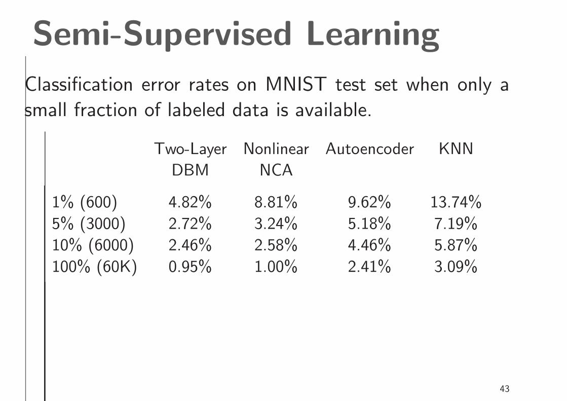
Semi-Supervised Learning

Classification error rates on MNIST test set when only a

small fraction of labeled data is available.

Two-Layer Nonlinear Autoencoder KNN

DBM NCA

1% (600) 4.82% 8.81% 9.62% 13.74%

5% (3000) 2.72% 3.24% 5.18% 7.19%

10% (6000) 2.46% 2.58% 4.46% 5.87%

100% (60K) 0.95% 1.00% 2.41% 3.09%

43

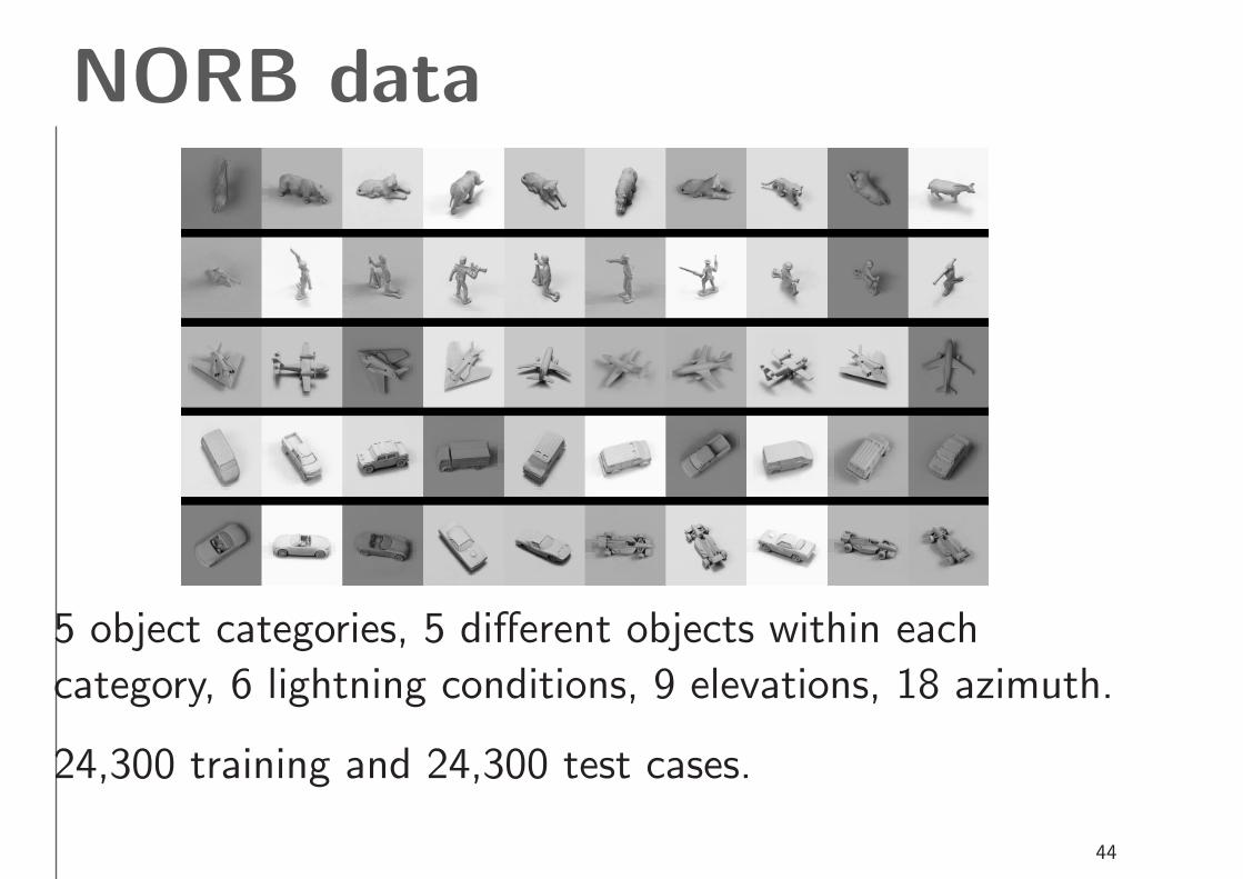
NORB data

5 object categories, 5 different objects within each

category, 6 lightning conditions, 9 elevations, 18 azimuth.

24,300 training and 24,300 test cases.

44

Deep Boltzmann Machines

4000 units

4000 units

4000 units

⇐=

Stereo pair

About 68 million parameters.

45

Model Samples

Discriminative fine-tuning: test error of 7.2%.

SVM’s get 11.6%, logistic regression gets 22.5%.

46

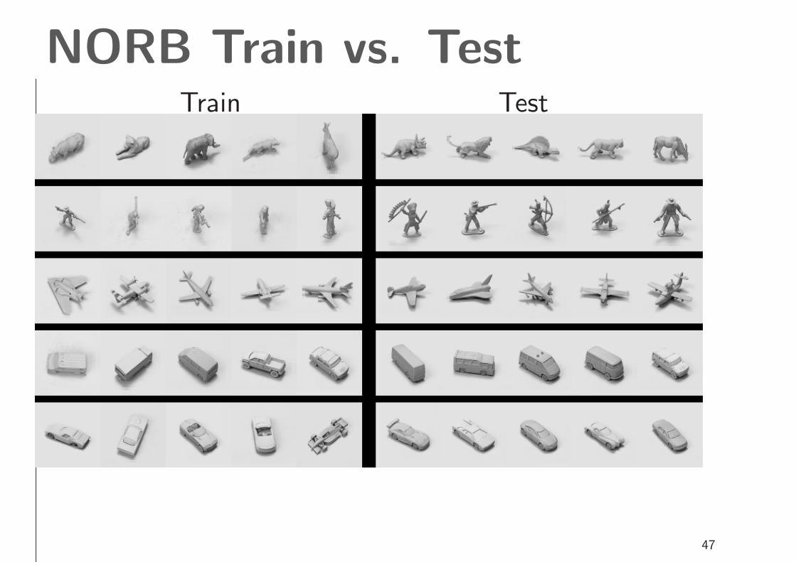
NORB Train vs. TestTrain Test

47

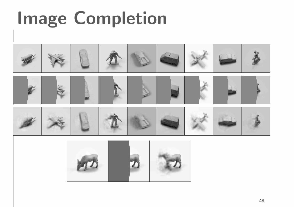
Image Completion

48

Extensions• Better Learning Algorithms for Deep Models:

– Better MCMC algorithms within stochastic approximation

that can explore highly mutimodal distributions: Tempered

Transitions, Simulated/Parallel Tempering.

– Faster and more accurate variational inference: loopy belief

propagation, generalized BP, power expectation propagation.

• Kernel Learning: Deep models can be used to define kernel

or similarity function for many discriminative methods, including

logistic regression, SVM’s, kernel regression, Gaussian processes.

49

Extensions• Large Scale Object Recognition and Information

Retrieval: Deep models have the potential to extract features

that become progressively more complex, which is a promising way

to solve object recognition and information retrieval problems.

• Discovering a hierarchical structure of object

categories: Learned high-level representations can be used as

the input to more structured hierarchical Bayesian models, which

would allow us to better incorporate our prior knowledge.

• Extracting Structure from Time: Modeling complex

nonlinear dynamics of high-dimensional time series data, such as

video sequences

50

Thank you.

51

Learning DBN’s

h

v

W

h1

h2

v

W1

W1⊤

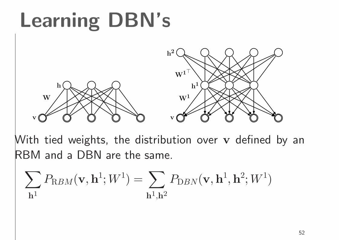
With tied weights, the distribution over v defined by an

RBM and a DBN are the same.∑

h1

PRBM(v,h1;W 1) =∑

h1,h2

PDBN(v,h1,h2;W 1)

52

Learning DBN’s

h

v

W

h1

h2

v

W1

W1⊤

log P (v; θ) ≥∑

h1

Q(h1|v)

[

log P (v,h1; θ)

]

+ H(Q(h1|v))

=∑

h1

Q(h1|v)

[

log P (h1; W 2) + log P (v|h1; W 1)

]

+ H(Q(h1|v))

Freeze Q(h1|v), and P (v|h1;W 1) and maximize the lower bound

w.r.t. P (h1;W 2).

53

Deep Belief Nets

P (v,h; θ) = P (v|h1)P (h1|h2)P (h2,h3).

v

h2

h1

h3

W1

W3

W2

h = {h1,h2,h3},

P (v; θ) =∑

h

P (v,h; θ).

Set of visible v and hidden h

binary stochastic units.

θ = {W 1,W 2,W 3} are model

parameters.

Inference and maximum likelihood learning are hard.

54