Deep Learning of Graph Matching

Andrei Zanfir2 and Cristian Sminchisescu1,2

andrei.zanfir@imar.ro, cristian.sminchisescu@math.lth.se1Department of Mathematics, Faculty of Engineering, Lund University

2Institute of Mathematics of the Romanian Academy

Abstract

The problem of graph matching under node and pair-wise constraints is fundamental in areas as diverse as com-binatorial optimization, machine learning or computer vi-sion, where representing both the relations between nodesand their neighborhood structure is essential. We present anend-to-end model that makes it possible to learn all param-eters of the graph matching process, including the unaryand pairwise node neighborhoods, represented as deep fea-ture extraction hierarchies. The challenge is in the formula-tion of the different matrix computation layers of the modelin a way that enables the consistent, efficient propagationof gradients in the complete pipeline from the loss func-tion, through the combinatorial optimization layer solvingthe matching problem, and the feature extraction hierar-chy. Our computer vision experiments and ablation studieson challenging datasets like PASCAL VOC keypoints, Sin-tel and CUB show that matching models refined end-to-endare superior to counterparts based on feature hierarchiestrained for other problems.

1. Introduction and Related WorkThe problem of graph matching – establishing corre-

spondences between two graphs represented in terms ofboth local node structure and pair-wise relationships, bethem visual, geometric or topological – is important in ar-eas like combinatorial optimization, machine learning, im-age analysis or computer vision, and has applications instructure-from-motion, object tracking, 2d and 3d shapematching, image classification, social network analysis, au-tonomous driving, and more. Our emphasis in this paperis on matching graph-based image representations but themethodology applies broadly, to any graph matching prob-lem where the unary and pairwise structures can be repre-sented as deep feature hierarchies with trainable parameters.

Unlike other methods such as RANSAC [12] or itera-tive closest point [4], which are limited to rigid displace-ments, graph matching naturally encodes structural infor-

mation that can be used to model complex relationshipsand more diverse transformations. Graph matching oper-ates with affinity matrices that encode similarities betweenunary and pairwise sets of nodes (points) in the two graphs.Typically it is formulated mathematically as a quadratic in-teger program [25, 3], subject to one-to-one mapping con-straints, i.e. each point in the first set must have an uniquecorrespondence in the second set. This is known to be NP-hard so methods often solve it approximately by relaxingthe constraints and finding local optima [19, 38].

Learning the parameters of the graph affinity matrix hasbeen investigated by [7, 20] or, in the context of the moregeneral hyper-graph matching model [10], by [21]. In thosecases, the number of parameters is low, often controlling ge-ometric affinities between pairs of points rather than the im-age structure in the neighborhood of those points. Recentlythere has been a growing interest in using deep features forboth geometric and semantic visual matching tasks, eitherby training the network to directly optimize a matching ob-jective [8, 27, 16, 36] or by using pre-trained, deep features[23, 14] within established matching architectures, all withconsiderable success.

Our objective in this paper is to marry the (shallow)graph matching to the deep learning formulations. We pro-pose to build models where the graphs are defined overunary node neighborhoods and pair-wise structures com-puted based on learned feature hierarchies. We formulate acomplete model to learn the feature hierarchies so that graphmatching works best: the feature learning and the graphmatching model are refined in a single deep architecturethat is optimized jointly for consistent results. Methodolog-ically, our contributions are associated to the construction ofthe different matrix layers of the computation graph, obtain-ing analytic derivatives all the way from the loss functiondown to the feature layers in the framework of matrix back-propagation, the emphasis on computational efficiency forbackward passes, as well as a voting based loss function.The proposed model applies generally, not just for match-ing different images of a category, taken in different scenes(its primary design), but also to different images of the same

scene, or from a video.

2. Problem FormulationInput. We are given two input graphs G1 = (V1, E1) andG2 = (V2, E2), with |V1| = n and |V2| = m. Our goalis to establish an assignment between the nodes of the twographs, so that a criterion over the corresponding nodes andedges is optimized (see below).

Graph Matching. Let v ∈ {0, 1}nm×1 be an indica-tor vector such that via = 1 if i ∈ V1 is matched toa ∈ V2 and 0 otherwise, while respecting one-to-one map-ping constraints. We build a square symmetric positive ma-trix M ∈ Rnm×nm such that Mia;jb measures how wellevery pair (i, j) ∈ E1 matches with (a, b) ∈ E2. For pairsthat do not form edges, their corresponding entries in thematrix are set to 0. The diagonal entries contain node-to-node scores, whereas the off-diagonal entries contain edge-to-edge scores. The optimal assignment v∗ can be formu-lated as

v∗ = argmaxv

v>Mv, s.t. Cv = 1,v ∈ {0, 1}nm×1 (1)

The binary matrix C ∈ Rnm×nm encodes one-to-one map-ping constraints: ∀a

∑i via = 1 and ∀i

∑a via = 1. This

is known to be NP-hard, so we relax the problem by drop-ping both the binary and the mapping constraints, and solve

v∗ = argmaxv

v>Mv, s.t. ‖v‖2 = 1 (2)

The optimal v∗ is then given by the leading eigenvector ofthe matrix M. Since M has non-negative elements, by us-ing Perron-Frobenius arguments, the elements of v∗ are inthe interval [0, 1], and we interpret v∗ia as the confidencethat i matches a.

Learning. We estimate the matrix M parameterized interms of unary and pair-wise point features computed overinput images and represented as deep feature hierarchies.We learn the feature hierarchies end-to-end in a loss func-tion that also integrates the matching layer. Specifically,given a training set of correspondences between pairs ofimages, we adapt the parameters so that the matching min-imizes the error, measured as a sum of distances betweenpredicted and ground truth correspondences. In our exper-iments, we work with graphs constructed over points thatcorrespond to the 2d image projections of the 3d structureof the same physical object in motion (in the context ofvideos), or over point configurations that correspond to thesame semantic category (matching instances of visual cat-egories, e.g. different birds). The main challenge is thepropagation of derivatives of the loss function through a fac-torization of the affinity matrix M, followed by matching

(in our formulation, this is an optimization problem, solvedusing eigen-decomposition) and finally the full feature ex-traction hierarchy used to compute the unary and pair-wisepoint representations.

2.1. Derivation Preliminaries

In practice, we build an end-to-end deep network thatintegrates a feature extracting component that outputs therequired descriptors F for building the matrix M. We solvethe assignment problem (2) and compute a matching lossL(v∗) between the solution v∗ and the ground-truth. Thenetwork must be able to pass gradients w.r.t the loss functionfrom the last to the first layer. The key gradients to compute– which we cover in §3 – are ∂L/∂M and ∂L/∂F. Thiscomputation could be difficult in the absence of an appro-priate factorization, as the computational and memory costsbecome prohibitive. Moreover, as some of our layers im-plement complex matrix functions, a matrix generalizationof back-propagation is necessary [15] for systematic deriva-tions and computational efficiency. In the sequel we coverits main intuition and refer to [15] for details.

Matrix backpropagation. We denote A : B =Tr(A>B) = vec(A)vec(B)>. For matrix derivatives, ifwe denote by f a function that outputs f(X) = Y and byL the network loss, the basis for the derivation starts fromthe Taylor expansion of the matrix functions [26] at the twolayers. By deriving the functional L expresssing the totalvariation dY in terms of dX,

dY = L(dX) (3)

and then using that

∂L ◦ f∂X

: dX =∂L

∂Y: L(dX) = L∗( ∂L

∂Y) : dX (4)

we obtain the equality ∂(L◦f)/∂X = L∗(∂L/∂Y), whereL∗ is the adjoint operator of L. This recipe for finding thepartial derivatives is used across all of our network layers.The derivations of L and L∗ are layer-specific and are givenin the following sections.

2.2. Affinity Matrix Factorization

Zhou and De la Torre [38] introduced a novel factoriza-tion of the matrix M that is generally applicable to all state-of-the-art graph matching methods. It explicitly exposes thegraph structure of the set of points and the unary and pair-wise scores between nodes and edges, respectively,

M = [vec(Mp)] + (G2 ⊗G1)[vec(Me)](H2 ⊗H1)>

(5)

where [x] represents the diagonal matrix with x on themain diagonal, and ⊗ is the Kronecker product. The matrix

Mp ∈ Rn×m represents the unary term, measuring node-to-node similarities, whereas Me ∈ Rp×q measures edge-to-edge similarity; p, q are the numbers of edges in eachgraph, respectively. The two matrices encode the first-orderand second-order potentials. To describe the structure ofeach graph, we define, as in [38], the node-edge incidencematrices as G,H ∈ {0, 1}n×p, where gic = hjc = 1 ifthe cth edge starts from the ith node and ends at the jth

node. We have two pairs, {G1,H1} ∈ {0, 1}n×p and{G2,H2} ∈ {0, 1}m×q , one for each image graph.

One simple way to build Me and Mp is

Me = XΛY>,Mp = U1U2> (6)

where X ∈ Rp×2d and Y ∈ Rq×2d are the per-edge featurematrices, constructed such that for any cth edge that startsfrom the ith node and ends at the jth node, we set the edgedescriptor as the concatenation of the descriptors extractedat the two nodes

Xc = [F1i |F1

j ],Yc = [F2i |F2

j ] (7)

The matrices F1,U1 ∈ Rn×d and F2,U2 ∈ Rm×d containper-node feature vectors of dimension d, extracted at possi-bly different levels in the network, and Λ is a 2d×2d block-symmetric parameter matrix. Superscripts 1, 2 indicate overwhich input image (source or target) are the features com-puted.

3. Deep Network Optimization for GraphMatching

In this section we describe how to integrate and learnthe graph matching model end-to-end, by implementing therequired components in an efficient way. This allows us toback-propagate gradients all the way from the loss functiondown to the feature layers. The main components of ourapproach are shown in Fig. 1.

3.1. Affinity Matrix Layer

If we define the node-to-node adjacency matrices A1 ∈{0, 1}n×n,A2 ∈ {0, 1}m×m, with aij = 1 if there is anedge from the ith node to the jth node, then

A1 = G1H>1 ,A2 = G2H

>2 (8)

The Affinity Matrix layer receives as input the required hi-erarchy of features, and the adjacency matrices A1 and A2

used to reconstruct the optimal G1,H1,G2,H2 matrices,which verify the equations (8). It is easier to describe theconnectivity of the graphs by adjacency matrices than bynode-edge incidence matrices, but we still need the latter forefficient backward passes at higher layers of the network.Next, we describe the forward and the backward passes ofthis layer, as parts of the trainable deep network.

Forward pass.

1. Given A1, A2, recover the matrices G1, H1, G2, H2,such that A1 = G1H

>1 ,A2 = G2H

>2

2. Given F1,F2, build X,Y according to (7)

3. Build Me = XΛY>

4. Given U1,U2, build Mp = U1U2>

5. Build M according to (5) and make G1,H1,G2,H2

available for the upper layers

Backward pass. Assuming the network provides∂L/∂Me and ∂L/∂Mp, this layer must return ∂L/∂F1,∂L/∂F2, ∂L/∂U1 and ∂L/∂U2; it must also compute∂L/∂Λ in order to update the matrix Λ. We assume∂L/∂Me and ∂L/∂Mp as input, and not ∂L/∂M,because the subsequent layer can take advantage of thisspecial factorization for efficient computation. We note thatmatrix Λ must have the following form in order for M tobe symmetric with positive elements

Λ =

(Λ1 Λ2

Λ2 Λ1

),Λij > 0,∀i, j (9)

Writing the variation of the loss layer in terms of the varia-tion of edge matrix and using the recipe (4),

dL =∂L

∂Me: dMe =

∂L

∂Me: d(XΛY>)

=∂L

∂Me: (dXΛY> + XdΛY> + XΛdY>)

=∂L

∂MeYΛ> : dX + X>

∂L

∂MeY : dΛ+

+∂L

∂Me

>XΛ : dY (10)

We identify the terms

∂L

∂X=

∂L

∂MeYΛ>

∂L

∂Λ= X>

∂L

∂MeY

∂L

∂Y=

∂L

∂MeXΛ (11)

To compute the partial derivatives ∂L/∂F1 and ∂L/∂F2,we identify and sum up the corresponding 1× d sub-blocksin the matrices ∂L/∂X and ∂L/∂Y. The partial derivative∂L/∂Λ is used to compute the derivatives ∂L/∂Λ1 and∂L/∂Λ2. Note that in implementing the positivity condi-tion from (9), one can use a ReLU unit.

Deep Feature Extractor

In: I1, I2Out: features matrices F1,F2 andU1,U2 as computed by any CNN,

at certain levels of the hierarchy,e.g. VGG-16 [29]

→

Affinity Matrix

In: F1,F2,U1,U2

Build graph structure:G1,G2,H1,H2

Computations: build Me and Mp

Out: M as given by eq. (5)

→

Power Iteration

In: MComputations: v0 ← 1,vk+1 = Mvk/ |Mvk|

Out: v∗

→

→

Bi-Stochastic

In: v∗

Computations: reshape v∗ to amatrix and apply eqs. (19)

Out: double-stochasticconfidence matrix S

→

Voting

In: S ∈ Rn×m

Computations: softmax(αS)Parameters: scale α

Out: displacement vector d asgiven by eq. (22)

→Loss

In: d,dgt

Out: L(d) =∑

i φ(di − dgti )

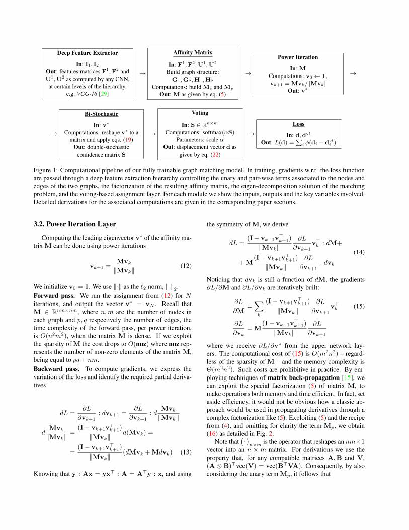
Figure 1: Computational pipeline of our fully trainable graph matching model. In training, gradients w.r.t. the loss functionare passed through a deep feature extraction hierarchy controlling the unary and pair-wise terms associated to the nodes andedges of the two graphs, the factorization of the resulting affinity matrix, the eigen-decomposition solution of the matchingproblem, and the voting-based assignment layer. For each module we show the inputs, outputs and the key variables involved.Detailed derivations for the associated computations are given in the corresponding paper sections.

3.2. Power Iteration Layer

Computing the leading eigenvector v∗ of the affinity ma-trix M can be done using power iterations

vk+1 =Mvk

‖Mvk‖(12)

We initialize v0 = 1. We use ‖·‖ as the `2 norm, ‖·‖2.Forward pass. We run the assignment from (12) for Niterations, and output the vector v∗ = vN . Recall thatM ∈ Rnm×nm, where n,m are the number of nodes ineach graph and p, q respectively the number of edges, thetime complexity of the forward pass, per power iteration,is O(n2m2), when the matrix M is dense. If we exploitthe sparsity of M the cost drops to O(nnz) where nnz rep-resents the number of non-zero elements of the matrix M,being equal to pq + nm.Backward pass. To compute gradients, we express thevariation of the loss and identify the required partial deriva-tives

dL =∂L

∂vk+1: dvk+1 =

∂L

∂vk+1: d

Mvk

‖Mvk‖

dMvk

‖Mvk‖=

(I− vk+1v>k+1)

‖Mvk‖d(Mvk) =

=(I− vk+1v

>k+1)

‖Mvk‖(dMvk + Mdvk) (13)

Knowing that y : Ax = yx> : A = A>y : x, and using

the symmetry of M, we derive

dL =(I− vk+1v

>k+1)

‖Mvk‖∂L

∂vk+1v>k : dM+

+ M(I− vk+1v

>k+1)

‖Mvk‖∂L

∂vk+1: dvk

(14)

Noticing that dvk is still a function of dM, the gradients∂L/∂M and ∂L/∂vk are iteratively built:

∂L

∂M=∑k

(I− vk+1v>k+1)

‖Mvk‖∂L

∂vk+1v>k (15)

∂L

∂vk= M

(I− vk+1v>k+1)

‖Mvk‖∂L

∂vk+1

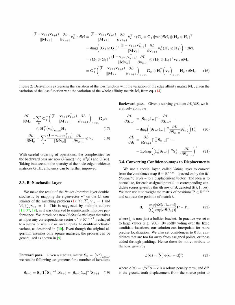
where we receive ∂L/∂v∗ from the upper network lay-ers. The computational cost of (15) is O(m2n2) – regard-less of the sparsity of M – and the memory complexity isΘ(m2n2). Such costs are prohibitive in practice. By em-ploying techniques of matrix back-propagation [15], wecan exploit the special factorization (5) of matrix M, tomake operations both memory and time efficient. In fact, setaside efficiency, it would not be obvious how a classic ap-proach would be used in propagating derivatives through acomplex factorization like (5). Exploiting (5) and the recipefrom (4), and omitting for clarity the term Mp, we obtain(16) as detailed in Fig. 2.

Note that(·)n×m is the operator that reshapes an nm×1

vector into an n × m matrix. For derivations we use theproperty that, for any compatible matrices A,B and V,(A ⊗ B)>vec(V) = vec(B>VA). Consequently, by alsoconsidering the unary term Mp, it follows that

(I− vk+1v>k+1)

‖Mvk‖∂L

∂vk+1v>k : dM =

(I− vk+1v>k+1)

‖Mvk‖∂L

∂vk+1v>k : (G2 ⊗G1)[vec(dMe)](H2 ⊗H1)>

= diag(

(G2 ⊗G1)>(I− vk+1v

>k+1)

‖Mvk‖∂L

∂vk+1v>k (H2 ⊗H1)

): dMe

= (G2 ⊗G1)>(I− vk+1v

>k+1)

‖Mvk‖∂L

∂vk+1� (H2 ⊗H1)>vk : dMe

= G>1

((I− vk+1v

>k+1)

‖Mvk‖∂L

∂vk+1

)n×m

G2 �H>1

(vk

)n×m

H2 : dMe (16)

Figure 2: Derivations expressing the variation of the loss function w.r.t the variation of the edge affinity matrix Me, given thevariation of the loss function w.r.t the variation of the whole affinity matrix M, from eq. (14)

∂L

∂Me=∑k

G>1

((I− vk+1v

>k+1)

‖Mvk‖∂L

∂vk+1

)n×m

G2�

�H>1(vk

)n×mH2 (17)

∂L

∂Mp=∑k

(I− vk+1v>k+1)

‖Mvk‖∂L

∂vk+1� vk (18)

With careful ordering of operations, the complexities forthe backward pass are now O(max(m2q, n2p)) and Θ(pq).Taking into account the sparsity of the node-edge incidencematrices G,H, efficiency can be further improved.

3.3. Bi-Stochastic Layer

We make the result of the Power Iteration layer double-stochastic by mapping the eigenvector v∗ on the L1 con-straints of the matching problem (1): ∀a,

∑i via = 1 and

∀i,∑

a via = 1. This is suggested by multiple authors[13, 37, 19], as it was observed to significantly improve per-formance. We introduce a new Bi-Stochastic layer that takesas input any correspondence vector v∗ ∈ Rnm×1

+ , reshapedto a matrix of size n×m, and outputs the double-stochasticvariant, as described in [30]. Even though the original al-gorithm assumes only square matrices, the process can begeneralized as shown in [9].

Forward pass. Given a starting matrix S0 =(v∗)n×m,

we run the following assignments for a number of iterations

Sk+1 = Sk[1>n Sk]−1,Sk+2 = [Sk+11m]−1Sk+1 (19)

Backward pass. Given a starting gradient ∂L/∂S, we it-eratively compute

∂L

∂Sk+1= [Sk+21m]−1

∂L

∂Sk+2−

− diag(

[Sk+21m]−2∂L

∂Sk+2S>k+2

)1>m (20)

∂L

∂Sk=

∂L

∂Sk+1[1>n Sk+1]−1−

− 1ndiag(

[1>n Sk+1]−2S>k+1

∂L

∂Sk+1

)>(21)

3.4. Converting Confidence-maps to Displacements

We use a special layer, called Voting layer to convertfrom the confidence map S ∈ Rn×m – passed on by the Bi-Stochastic layer – to a displacement vector. The idea is tonormalize, for each assigned point i, its corresponding can-didate scores given by the ith row of S, denoted S(i, 1...m).We then use it to weight the matrix of positions P ∈ Rm×2

and subtract the position of match i.

di =exp[αS(i, 1...m)]∑

j exp[αS(i, j)]P−Pi (22)

where [] is now just a bulkier bracket. In practice we set αto large values (e.g. 200). By softly voting over the fixedcandidate locations, our solution can interpolate for moreprecise localization. We also set confidences to 0 for can-didates that are too far away from assigned points, or thoseadded through padding. Hence these do not contribute tothe loss, given by

L(d) =∑i

φ(di − dgti ) (23)

where φ(x) =√

x>x + ε is a robust penalty term, and dgt

is the ground-truth displacement from the source point to

the correct assignment. This layer is implemented in mul-tiple, fully differentiable steps: a) first, scale the input byα, b) use a spatial map for discarding candidate locationsthat are further away than a certain threshold from the start-ing location and use it to modify the confidence maps, c)use a softmax layer to normalize the confidence maps, d)compute the displacement map. The discard map sets theconfidences to 0 for points that are further away than a cer-tain distance, or for points that were added through padding.Such points do not contribute in the final loss, given by (23).

4. ExperimentsIn this section we describe the models used as well as de-

tailed experimental matching results, both quantitative (in-cluding ablation studies) and qualitative, on three challeng-ing datasets: MPI Sintel, CUB, and PASCAL keypoints.

Deep feature extraction network. We rely on the VGG-16 architecture from [29], that is pretrained to perform clas-sification in the ImageNet ILSVRC [28] but we can useany other deep network architecture. We implement ourdeep learning framework in MatConvNet [31]. As edgefeatures F we use the output of layer relu5_1 (and theentire hierarchy under it), and for the node features U weuse the output of layer relu4_2 (with the parameters ofthe associated hierarchy under it). Features are all normal-ized to 1 through normalization layers, right before they areused to compute the affinity matrix M. We conduct experi-ments for geometric and semantic correspondences on MPI-Sintel [6], Caltech-UCSD Birds-200-2011 [32] and PAS-CAL VOC [11] with Berkeley annotations [5].

Matching networks. GMNwVGG is our proposed GraphMatching Network based on a VGG feature extractor. Thesuffix -U means that default (initial) weights are used; -Tmeans trained end-to-end; the GMNwVGG-T w/o V variantdoes not use, at testing, the Voting layer in order to computethe displacements, but directly assigns indices of maximumvalue across the rows of the confidence map S, as corre-spondences. NNwVGG gives nearest-neighbour matchingbased on deep node descriptors U.

MPI-Sintel. Besides the main datasets CUB and PAS-CAL, typically employed in validating matching methods,we also use Sintel in order to demonstrate the generalityand flexibility of the formulation. The Sintel input imagesare consecutive frames in a movie and exhibit large dis-placements, large appearance changes, occlusion, non-rigidmovements and complex atmospheric effects (only includedin the final set of images). The Sintel training set consists of23 video sequences (organized as folders) and 1064 frames.In order to make sure that we are fairly training and eval-uating, as images from the same video depict instances of

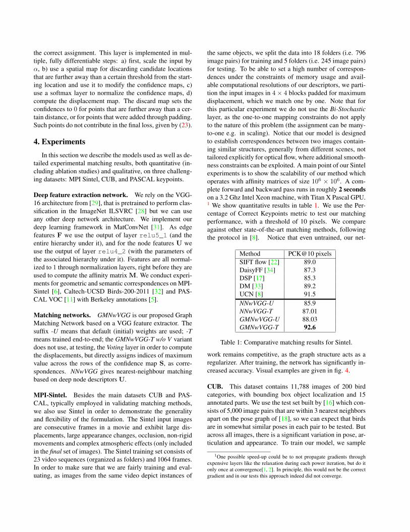
the same objects, we split the data into 18 folders (i.e. 796image pairs) for training and 5 folders (i.e. 245 image pairs)for testing. To be able to set a high number of correspon-dences under the constraints of memory usage and avail-able computational resolutions of our descriptors, we parti-tion the input images in 4× 4 blocks padded for maximumdisplacement, which we match one by one. Note that forthis particular experiment we do not use the Bi-Stochasticlayer, as the one-to-one mapping constraints do not applyto the nature of this problem (the assignment can be many-to-one e.g. in scaling). Notice that our model is designedto establish correspondences between two images contain-ing similar structures, generally from different scenes, nottailored explicitly for optical flow, where additional smooth-ness constraints can be exploited. A main point of our Sintelexperiments is to show the scalability of our method whichoperates with affinity matrices of size 106 × 106. A com-plete forward and backward pass runs in roughly 2 secondson a 3.2 Ghz Intel Xeon machine, with Titan X Pascal GPU.1 We show quantitative results in table 1. We use the Per-centage of Correct Keypoints metric to test our matchingperformance, with a threshold of 10 pixels. We compareagainst other state-of-the-art matching methods, followingthe protocol in [8]. Notice that even untrained, our net-

Method PCK@10 pixelsSIFT flow [22] 89.0DaisyFF [34] 87.3DSP [17] 85.3DM [33] 89.2UCN [8] 91.5NNwVGG-U 85.9NNwVGG-T 87.01GMNwVGG-U 88.03GMNwVGG-T 92.6

Table 1: Comparative matching results for Sintel.

work remains competitive, as the graph structure acts as aregularizer. After training, the network has significantly in-creased accuracy. Visual examples are given in fig. 4.

CUB. This dataset contains 11,788 images of 200 birdcategories, with bounding box object localization and 15annotated parts. We use the test set built by [16] which con-sists of 5,000 image pairs that are within 3 nearest neighborsapart on the pose graph of [18], so we can expect that birdsare in somewhat similar poses in each pair to be tested. Butacross all images, there is a significant variation in pose, ar-ticulation and appearance. To train our model, we sample

1One possible speed-up could be to not propagate gradients throughexpensive layers like the relaxation during each power iteration, but do itonly once at convergence[1, 2]. In principle, this would not be the correctgradient and in our tests this approach indeed did not converge.

random pairs of images from the training set of CUB-200-2011, which are not present in the test set. The number ofpoints in the two graphs are maximum n = 15 andm = 256– as sampled from a 16×16 grid – with a Delaunay triangu-lation on the first graph, and fully connected on the second.In the Voting layer, we no longer discard candidate locationsthat are too far away from the source points. A completeforward and backward pass runs in 0.3 seconds.

Method EPE (in pixels) PCK@0.05GMNwVGG-U 41.63 0.63NNwVGG-U 59.05 0.46GMNwVGG-T w/o V 18.22 0.83GMNwVGG-T 17.02 0.86

Table 2: Our models (with ablations) on CUB.

We show quantitative results in table 2. The ”PCK@α”metric [35] represents the percentage of predicted corre-spondences that are closer than α

√w2 + h2 from ground-

truth locations, where w, h are image dimensions. Qualita-tive results are shown in fig. 5.

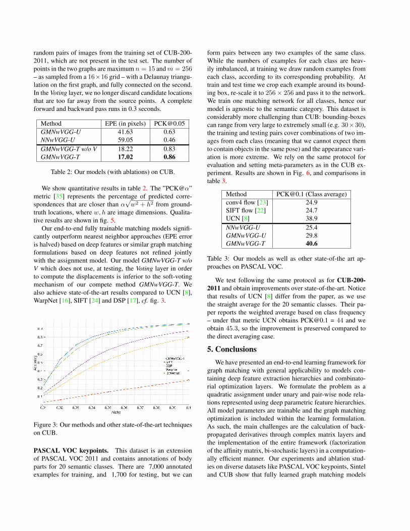
Our end-to-end fully trainable matching models signifi-cantly outperform nearest neighbor approaches (EPE erroris halved) based on deep features or similar graph matchingformulations based on deep features not refined jointlywith the assignment model. Our model GMNwVGG-T w/oV which does not use, at testing, the Voting layer in orderto compute the displacements is inferior to the soft-votingmechanism of our compete method GMNwVGG-T. Wealso achieve state-of-the-art results compared to UCN [8],WarpNet [16], SIFT [24] and DSP [17], cf. fig. 3.

Figure 3: Our methods and other state-of-the-art techniqueson CUB.

PASCAL VOC keypoints. This dataset is an extensionof PASCAL VOC 2011 and contains annotations of bodyparts for 20 semantic classes. There are 7,000 annotatedexamples for training, and 1,700 for testing, but we can

form pairs between any two examples of the same class.While the numbers of examples for each class are heav-ily imbalanced, at training we draw random examples fromeach class, according to its corresponding probability. Attrain and test time we crop each example around its bound-ing box, re-scale it to 256× 256 and pass it to the network.We train one matching network for all classes, hence ourmodel is agnostic to the semantic category. This dataset isconsiderably more challenging than CUB: bounding-boxescan range from very large to extremely small (e.g. 30×30),the training and testing pairs cover combinations of two im-ages from each class (meaning that we cannot expect themto contain objects in the same pose) and the appearance vari-ation is more extreme. We rely on the same protocol forevaluation and setting meta-parameters as in the CUB ex-periment. Results are shown in Fig. 6, and comparisons intable 3.

Method PCK@0.1 (Class average)conv4 flow [23] 24.9SIFT flow [22] 24.7UCN [8] 38.9NNwVGG-U 25.4GMNwVGG-U 29.8GMNwVGG-T 40.6

Table 3: Our models as well as other state-of-the art ap-proaches on PASCAL VOC.

We test following the same protocol as for CUB-200-2011 and obtain improvements over state-of-the-art. Noticethat results of UCN [8] differ from the paper, as we usethe straight average for the 20 semantic classes. Their pa-per reports the weighted average based on class frequency– under that metric UCN obtains PCK@0.1 = 44 and weobtain 45.3, so the improvement is preserved compared tothe direct averaging case.

5. ConclusionsWe have presented an end-to-end learning framework for

graph matching with general applicability to models con-taining deep feature extraction hierarchies and combinato-rial optimization layers. We formulate the problem as aquadratic assignment under unary and pair-wise node rela-tions represented using deep parametric feature hierarchies.All model parameters are trainable and the graph matchingoptimization is included within the learning formulation.As such, the main challenges are the calculation of back-propagated derivatives through complex matrix layers andthe implementation of the entire framework (factorizationof the affinity matrix, bi-stochastic layers) in a computation-ally efficient manner. Our experiments and ablation stud-ies on diverse datasets like PASCAL VOC keypoints, Sinteland CUB show that fully learned graph matching models

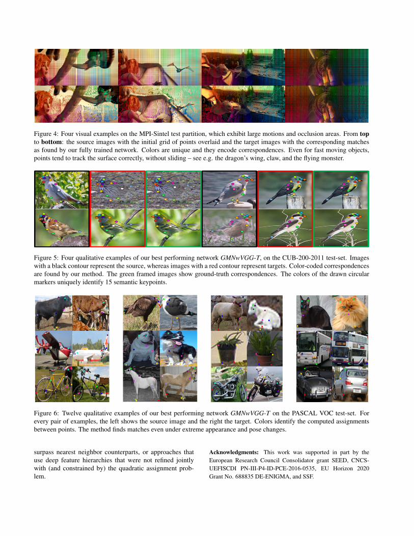
Figure 4: Four visual examples on the MPI-Sintel test partition, which exhibit large motions and occlusion areas. From topto bottom: the source images with the initial grid of points overlaid and the target images with the corresponding matchesas found by our fully trained network. Colors are unique and they encode correspondences. Even for fast moving objects,points tend to track the surface correctly, without sliding – see e.g. the dragon’s wing, claw, and the flying monster.

Figure 5: Four qualitative examples of our best performing network GMNwVGG-T, on the CUB-200-2011 test-set. Imageswith a black contour represent the source, whereas images with a red contour represent targets. Color-coded correspondencesare found by our method. The green framed images show ground-truth correspondences. The colors of the drawn circularmarkers uniquely identify 15 semantic keypoints.

Figure 6: Twelve qualitative examples of our best performing network GMNwVGG-T on the PASCAL VOC test-set. Forevery pair of examples, the left shows the source image and the right the target. Colors identify the computed assignmentsbetween points. The method finds matches even under extreme appearance and pose changes.

surpass nearest neighbor counterparts, or approaches thatuse deep feature hierarchies that were not refined jointlywith (and constrained by) the quadratic assignment prob-lem.

Acknowledgments: This work was supported in part by theEuropean Research Council Consolidator grant SEED, CNCS-UEFISCDI PN-III-P4-ID-PCE-2016-0535, EU Horizon 2020Grant No. 688835 DE-ENIGMA, and SSF.

References[1] B. Amos and J. Z. Kolter. Optnet: Differentiable optimiza-

tion as a layer in neural networks. CoRR, abs/1703.00443,2017.

[2] J. T. Barron and B. Poole. The fast bilateral solver. CoRR,abs/1511.03296, 2015.

[3] A. C. Berg, T. L. Berg, and J. Malik. Shape matchingand object recognition using low distortion correspondences.In Computer Vision and Pattern Recognition, 2005. CVPR2005. IEEE Computer Society Conference on, volume 1,pages 26–33. IEEE, 2005.

[4] P. J. Besl and N. D. McKay. Method for registration of 3-dshapes. In Robotics-DL tentative, pages 586–606. Interna-tional Society for Optics and Photonics, 1992.

[5] L. Bourdev and J. Malik. Poselets: Body part detectorstrained using 3d human pose annotations. In Computer Vi-sion, 2009 IEEE 12th International Conference on, pages1365–1372. IEEE, 2009.

[6] D. J. Butler, J. Wulff, G. B. Stanley, and M. J. Black. Anaturalistic open source movie for optical flow evaluation. InEuropean Conference on Computer Vision, pages 611–625.Springer, 2012.

[7] T. S. Caetano, J. J. McAuley, L. Cheng, Q. V. Le, and A. J.Smola. Learning graph matching. IEEE transactions onpattern analysis and machine intelligence, 31(6):1048–1058,2009.

[8] C. B. Choy, J. Gwak, S. Savarese, and M. Chandraker. Uni-versal correspondence network. In Advances in Neural In-formation Processing Systems, pages 2406–2414, 2016.

[9] T. Cour, P. Srinivasan, and J. Shi. Balanced graph matching.In NIPS, volume 2, page 6, 2006.

[10] O. Duchenne, F. Bach, I.-S. Kweon, and J. Ponce. Atensor-based algorithm for high-order graph matching. IEEEtransactions on pattern analysis and machine intelligence,33(12):2383–2395, 2011.

[11] M. Everingham and J. Winn. The pascal visual object classeschallenge 2011 (voc2011) development kit. Pattern Analy-sis, Statistical Modelling and Computational Learning, Tech.Rep, 2011.

[12] M. A. Fischler and R. C. Bolles. Random sample consen-sus: a paradigm for model fitting with applications to imageanalysis and automated cartography. Communications of theACM, 24(6):381–395, 1981.

[13] S. Gold and A. Rangarajan. A graduated assignment algo-rithm for graph matching. IEEE Transactions on patternanalysis and machine intelligence, 18(4):377–388, 1996.

[14] B. Ham, M. Cho, C. Schmid, and J. Ponce. Proposal flow.In Proceedings of the IEEE Conference on Computer Visionand Pattern Recognition, pages 3475–3484, 2016.

[15] C. Ionescu, O. Vantzos, and C. Sminchisescu. Training deepnetworks with structured layers by matrix backpropagation.arXiv preprint arXiv:1509.07838, 2015.

[16] A. Kanazawa, D. W. Jacobs, and M. Chandraker. Warpnet:Weakly supervised matching for single-view reconstruction.In Proceedings of the IEEE Conference on Computer Visionand Pattern Recognition, pages 3253–3261, 2016.

[17] J. Kim, C. Liu, F. Sha, and K. Grauman. Deformable spatialpyramid matching for fast dense correspondences. In Pro-ceedings of the IEEE Conference on Computer Vision andPattern Recognition, pages 2307–2314, 2013.

[18] J. Krause, H. Jin, J. Yang, and L. Fei-Fei. Fine-grainedrecognition without part annotations. In Proceedings of theIEEE Conference on Computer Vision and Pattern Recogni-tion, pages 5546–5555, 2015.

[19] M. Leordeanu and M. Hebert. A spectral technique for corre-spondence problems using pairwise constraints. In ComputerVision, 2005. ICCV 2005. Tenth IEEE International Confer-ence on, volume 2, pages 1482–1489. IEEE, 2005.

[20] M. Leordeanu, R. Sukthankar, and M. Hebert. Unsupervisedlearning for graph matching. International journal of com-puter vision, 96(1):28–45, 2012.

[21] M. Leordeanu, A. Zanfir, and C. Sminchisescu. Semi-supervised learning and optimization for hypergraph match-ing. In Computer Vision (ICCV), 2011 IEEE InternationalConference on, pages 2274–2281. IEEE, 2011.

[22] C. Liu, J. Yuen, and A. Torralba. Sift flow: Dense correspon-dence across scenes and its applications. IEEE Transactionson Pattern Analysis and Machine Intelligence, 33(5):978–994, 2011.

[23] J. L. Long, N. Zhang, and T. Darrell. Do convnets learn cor-respondence? In Advances in Neural Information ProcessingSystems, pages 1601–1609, 2014.

[24] D. G. Lowe. Distinctive image features from scale-invariant keypoints. International journal of computer vi-sion, 60(2):91–110, 2004.

[25] J. Maciel and J. P. Costeira. A global solution to sparse corre-spondence problems. IEEE Transactions on Pattern Analysisand Machine Intelligence, 25(2):187–199, 2003.

[26] J. R. Magnus, H. Neudecker, et al. Matrix differential calcu-lus with applications in statistics and econometrics. 1995.

[27] I. Rocco, R. Arandjelovic, and J. Sivic. Convolutional neuralnetwork architecture for geometric matching. arXiv preprintarXiv:1703.05593, 2017.

[28] O. Russakovsky, J. Deng, H. Su, J. Krause, S. Satheesh,S. Ma, Z. Huang, A. Karpathy, A. Khosla, M. Bernstein,et al. Imagenet large scale visual recognition challenge.International Journal of Computer Vision, 115(3):211–252,2015.

[29] K. Simonyan and A. Zisserman. Very deep convolutionalnetworks for large-scale image recognition. arXiv preprintarXiv:1409.1556, 2014.

[30] R. Sinkhorn and P. Knopp. Concerning nonnegative matricesand doubly stochastic matrices. Pacific Journal of Mathemat-ics, 21(2):343–348, 1967.

[31] A. Vedaldi and K. Lenc. Matconvnet – convolutional neuralnetworks for matlab. In Proceeding of the ACM Int. Conf. onMultimedia, 2015.

[32] C. Wah, S. Branson, P. Welinder, P. Perona, and S. Belongie.The Caltech-UCSD Birds-200-2011 Dataset. Technical Re-port CNS-TR-2011-001, California Institute of Technology,2011.

[33] P. Weinzaepfel, J. Revaud, Z. Harchaoui, and C. Schmid.Deepflow: Large displacement optical flow with deep match-

ing. In Computer Vision (ICCV), 2013 IEEE InternationalConference on, pages 1385–1392. IEEE, 2013.

[34] H. Yang, W. Lin, and J. Lu. Daisy filter flow: A generalizedapproach to discrete dense correspondences. CVPR, 2014.

[35] Y. Yang and D. Ramanan. Articulated human detectionwith flexible mixtures of parts. IEEE Transactions on Pat-tern Analysis and Machine Intelligence, 35(12):2878–2890,2013.

[36] K. M. Yi, E. Trulls, V. Lepetit, and P. Fua. Lift: Learned in-variant feature transform. In European Conference on Com-puter Vision, 2016.

[37] R. Zass and A. Shashua. Probabilistic graph and hyper-graph matching. In Computer Vision and Pattern Recog-nition, 2008. CVPR 2008. IEEE Conference on, pages 1–8.IEEE, 2008.

[38] F. Zhou and F. De la Torre. Factorized graph matching.In Computer Vision and Pattern Recognition (CVPR), 2012IEEE Conference on, pages 127–134. IEEE, 2012.