THE ROMANIAN ACADEMY

SIMION STOILOW INSTITUTE OF MATHEMATICS

Robust Estimation of VisualCorrespondence Fields and Dynamic

Scenes Structure

Author,Andrei ZANFIR

Supervisor,C.S. I Dr. Cristian SMINCHIS, ESCU

PH. D. THESIS SUMMARY

Bucharest2018

2

Chapter 1

Introduction

Establishing correspondences between similar structures (e.g. points) in different images

is a fundamental computer problem. It exposes the need for non-local image reasoning,

leveraging the underlying 3d geometry of the scene, and modeling the range of deforma-

tions that many objects – including deformable and articulated structures like people or

animals – are subject to. The applications are diverse, as current emerging technologies

rely on variants of image-to-image matching like optical flow, scene flow, sparse matching,

semantic matching, etc. Self-driving cars need to understand visual motion, drones have

to track objects and virtual reality devices need to build 3d geometrical models of the en-

vironment. Hence they require solutions to fundamental, yet challenging questions like:

When do two visual primitives are the instances of the same moving 3d structures? How

can two structures from the same semantic category, but with different appearance, can be

matched?

In this thesis we do not only propose models and solutions for image correspondence,

but we also offer insights and long-term directions for future research. Our models are de-

signed to address the current challenges in image matching including large-displacements

and fast-motions, repetitive structures, non-trivial lighting conditions, cluttered backgrounds,

intra-class variability, or large occlusion areas.

For computing optical flow, we propose a sparse-to-coarse method, that combines sparse

matching with a novel affine model and a geometric interpolation method, with competitive

results. We show that pursuing alternative models to the classical variational approach is

3

beneficial and has practical relevance.

We address the problem of scene flow, the 3d counter-part of optical flow, by addition-

ally exploiting the depth information collected from a depth sensor. By incorporating a

complete energy model that balances sparse matching, a 3d rigid model hypothesis, photo-

metric and depth consistency terms, we obtain state-of-the-art results, that can capture fast

motions and sharp boundaries.

We further propose a deep-learning formulation of matching, where we design and

train a model to minimize a graph-matching objective, that combines unary and pairwise

node neighborhood relations. This novel approach poses considerable mathematical chal-

lenges, as the derivatives need to be passed across complete structured layers (like opti-

mization modules with solutions based on e.g. relaxations) accurately, following matrix

back-propagation rules. We construct a complex, fully trainable framework, and show im-

proved results for both geometric and semantic matching datasets. This latter work received

the best paper award honorable mention at IEEE CVPR 2018.

4

Chapter 2

Locally Affine Sparse-to-Dense

Matching for Motion and Occlusion

Estimation

This chapter is based on ”Locally Affine Sparse-to-Dense Matching for Motion and Occlu-

sion Estimation” Marius Leordeanu, Andrei Zanfir and Cristian Sminchis, escu, in the IEEE

International Conference on Computer Vision, Sydney, Australia, December 2013.

2.1 Introduction

Estimating a dense correspondence field between subsequent video frames is important

to many visual learning and recognition tasks. Here we propose a novel sparse-to-dense

matching method for motion field estimation with occlusion detection. As an alternative

to the current coarse-to-fine approaches from the optical flow literature, we start from the

higher level of sparse matching with rich appearance and geometric constraints, using a

novel, occlusion aware, locally affine model. Then, we move towards the simpler, but

denser classic flow field model, with a novel sparse-to-dense matching interpolation pro-

cedure that offers a natural transition between the sparse and dense correspondence fields.

We demonstrate experimentally that our appearance features and complex geometric con-

straints permit the correct motion estimation even in difficult cases of large displacements

5

Figure 2-1: Left: motion fields estimated at different stages of our method. Right: flowchartof our approach. Sparse matching results are resized to original image size for displaypurposes.

and significant appearance changes. We also propose a classification method for occlu-

sion detection that works in conjunction with sparse-to-dense matching. We validate our

approach on the newly released Sintel dataset, on which we obtain state-of-the-art results.

Overview of our approach: We propose a hierarchical sparse-to-dense matching method

that integrates and generalizes ideas from both the traditional coarse-to-fine variational

approach and more recent methods using sparse feature matching [1, 7, 4, 3, 14, 8]. Our

method consists of three main phases (Figure 2-1):

1. Sparse Matching: Initialize a discrete set of candidate matches for each point on

a sparse grid (in the first image) using dense kNN matching (in the second image)

with local feature descriptors. Use the output of a boundary detector and cues from

the initial sparse matching to infer a first occlusion probability map. Then discretely

optimize a sparse matching cost function using both unary data terms (from local

features) and geometric relationships based on a locally affine model with occlusion

constraints. Use the improved matches to refine the occlusion map.

2. Sparse-to-Dense Interpolation: Fix the sparse matches from the previous step.

6

Then apply the same occlusion sensitive geometric model to obtain an accurate

sparse-to-dense matching interpolation.

3. Dense matching refinement: use a TV model with continuous flow optimization to

obtain the final dense correspondence field. Use matching cues computed from all

stages to obtain the final occlusion map.

2.1.1 Locally Affine Spatial Model

The key contribution of our paper is the locally affine spatial prior that we propose. The

intuition is that points that are likely to be on the same object surface and are close to each

other are also likely to have a similar displacement. The motions of such points within a

certain neighborhood are expected to closely follow an affine transformation. To model

this idea, we first define a geometric neighborhood system over the grid locations (see

Figure 2-2), and link neighboring points (i, j) using an edge strength function eij - meant

to measure the probability that two points lie on the same object surface and obey a similar

affine transformation from I1 to I2.

We use the locations of i’s neighbors, p(1)Ni

in I1, their current estimated destinations

in I2, p(2)Ni

, and their membership weights, to estimate a motion model that predicts the

destination p(2)i of the current point i in I2: p

(2)i = TNi

(p(1)i ). Then, the prediction error

between the current p(2)i (wi) = p

(1)i + wi and the estimated p

(2)i forms the basis of our

spatial term:

ES(w) =∑i

‖p(2)i (w)− TNi

(p(1)i )‖2. (2.1)

In our particular case, when TNiis a local affine transformation, Eq. 2.1 reduces to a second

order energy that can be efficiently optimized.

For each point iwe estimate its affine transformation TNi= (Ai, ti) from its neighbors’

motions by weighted least squares, with weights eij, ∀j ∈ Ni. Let 2Ni × 1 pNi= p

(2)Ni

be

the estimated positions of its neighbors in I2 and M the Moore-Penrose pseudo-inverse of

the least squares problem, which depends only on the locations of the neighbors p(1)Ni

, and

their weights.

7

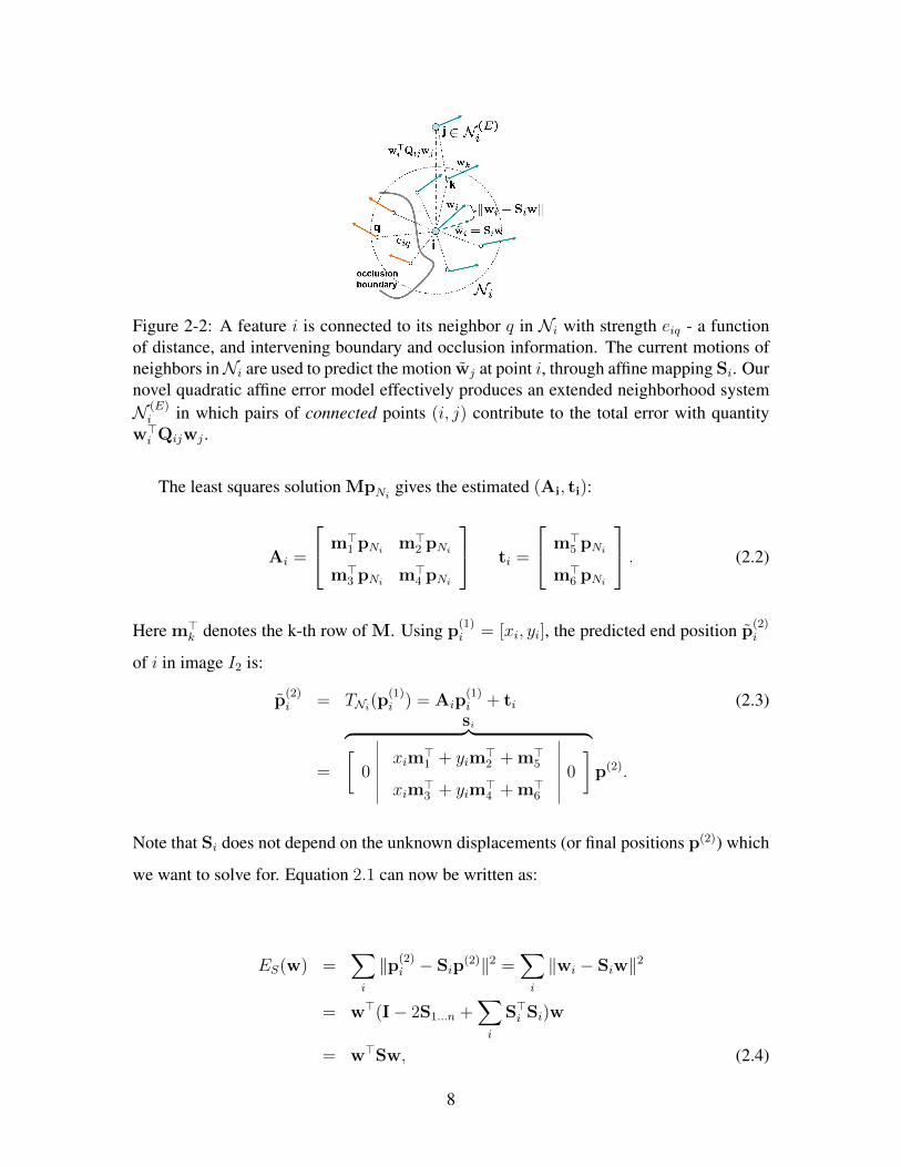
Figure 2-2: A feature i is connected to its neighbor q in Ni with strength eiq - a functionof distance, and intervening boundary and occlusion information. The current motions ofneighbors inNi are used to predict the motion wj at point i, through affine mapping Si. Ournovel quadratic affine error model effectively produces an extended neighborhood systemN (E)

i in which pairs of connected points (i, j) contribute to the total error with quantityw>i Qijwj .

The least squares solution MpNigives the estimated (Ai, ti):

Ai =

m>1 pNim>2 pNi

m>3 pNim>4 pNi

ti =

m>5 pNi

m>6 pNi

. (2.2)

Here m>k denotes the k-th row of M. Using p(1)i = [xi, yi], the predicted end position p

(2)i

of i in image I2 is:

p(2)i = TNi

(p(1)i ) = Aip

(1)i + ti (2.3)

=

Si︷ ︸︸ ︷[0

xim>1 + yim

>2 + m>5

xim>3 + yim

>4 + m>6

0

]p(2).

Note that Si does not depend on the unknown displacements (or final positions p(2)) which

we want to solve for. Equation 2.1 can now be written as:

ES(w) =∑i

‖p(2)i − Sip

(2)‖2 =∑i

‖wi − Siw‖2

= w>(I− 2S1...n +∑i

S>i Si)w

= w>Sw, (2.4)

8

Table 2.1: Final results on Sintel optical flow benchmark; epe stands for end point errors,epem are errors for visible points, and epeo are errors for occluded points. The last threecolumns show average errors for different motion magnitudes (in pixels).

Alg. epe epem epeo 0-10 10-40 40+S2D 7.88 3.91 40.16 1.17 4.66 48.90[14] 8.45 4.15 43.43 1.42 5.45 50.51[3] 9.12 5.04 42.34 1.49 4.84 57.30[12]-full 9.16 4.81 44.51 1.11 4.50 60.29[5] 9.61 5.42 43.73 1.88 5.34 58.27[12]++ 9.96 5.41 47.00 1.40 5.10 64.14[12]-fast 10.09 5.66 46.15 1.09 4.67 67.80[13] 11.93 7.32 49.37 1.16 7.97 74.80

This energy term ES(w) will be used by the sparse matching and the sparse-to-dense

interpolation stages to compute or update the solution w∗.

2.2 Experimental results

We show qualitative and quantitative results in fig. 2-3 and in table 2.1.

Figure 2-3: Motion field estimation results. Our algorithm can handle large displacements(in the sparse matching phase) while preserving motion details by TV continuous refine-ment at the last stage.

9

10

Chapter 3

Large Displacement 3D Scene Flow with

Occlusion Reasoning

This chapter is based on the paper ”Large Displacement 3D Scene Flow with Occlusion

Reasoning” Andrei Zanfir and Cristian Sminchis, escu, published in the IEEE International

Conference on Computer Vision, Santiago de Chile, Chile, December 2015

3.1 Introduction

The emergence of modern, affordable and accurate RGB-D sensors increases the need for

single view approaches to estimate 3-dimensional motion, also known as scene flow. In

this paper we propose a coarse-to-fine, dense, correspondence-based scene flow formula-

tion that relies on explicit geometric reasoning to account for the effects of large displace-

ments and to model occlusion. Our methodology enforces local motion rigidity at the level

of the 3d point cloud without explicitly smoothing the parameters of adjacent neighbor-

hoods. By integrating all geometric and photometric components in a single, consistent,

occlusion-aware energy model, defined over overlapping, image-adaptive neighborhoods,

our method can process fast motions and large occlusions areas, as present in challenging

datasets like the MPI Sintel Flow Dataset, recently augmented with depth information. By

explicitly modeling large displacements and occlusion, we can handle difficult sequences

which cannot be currently processed by state of the art scene flow methods. We also show

11

that by integrating depth information into the model, we can obtain correspondence fields

with improved spatial support and sharper boundaries compared to the state of the art,

large-displacement optical flow methods.

3.2 Model Formulation

We design a dense energy model that can handle large displacement and occlusion. The

model is expressed in terms of several energy sub-components. It relies on geometric large-

displacement correspondence anchors, local rigidity assumptions defined over large neigh-

borhoods constructed using the RGB-D point cloud, on appearance consistency, and depth

constancy terms. Geometric occlusion estimates are used in order to control the strength of

the neighborhood connections and automatically mask regions for which correspondences

cannot be established.

Rigid Parameter Fields. Our geometric model links the dense correspondences Y to the

initial points X by assuming an underlying field of rigid parameters Θ = [θ>1 ,θ>2 , ...,θ

>N ]>

, where θi = [v>i , t>i ]> are rigid parameters that constrain each neighborhood N (i) of a

point xi ∈ X. A neighborhood represents the closest K points to xi in 3d, where K is

chosen appropriately, according to the pyramid level.

The full energy model to optimize can be written as:

E(Y,Θ) = EA + αEZ + βEM + λEG (3.1)

where α, β and λ are weights estimated by validation.

Minimization. We solve (3.1) over the parameter fields Y,Θ by alternating variable opti-

mization:

Θk+1 ← argminΘ

E(Yk,Θk) (3.2)

Yk+1 ← argminY

E(Yk,Θk+1) (3.3)

where k is the iteration index. We run the optimization until convergence.

12

3.3 Experimental results

We show quantitative and qualitative results on state-of-the-art scene flow benchmarks in

table 3.1, in fig. 3-1 and in fig. 3-2.

Figure 3-1: Five pairs of images and four methods illustrated on the Sintel dataset: 1strow: input images overlaid, 2nd row: [2], 3rd row: [9] (N.B. this state of the art 3dscene flow method is not designed to handle large displacements, but produces excellentresults for small to moderate ones), see also fig. 3-2, 4th row: EpicFlow[10], 5th row: ourproposed approach shows sharper boundaries and improved spatial support estimates, 6throw: ground truth optical flow. On the last two rows we show the ground truth occlusionstates and our soft estimates.

Algorithms LDOF[2] EpicFlow[10] OursError(in pixels) 7.44 4.82 4.6

Table 3.1: Quantitative evaluation of state of the art 2d and 3d methods on the challeng-ing Sintel dataset (Sintel-Test92). Our method uses 3d information and offers improvedaccuracy as well as accurate estimates of occlusion.

13

Figure 3-2: Sample scene flow estimation with results in the x-y plane for image pairsin the Sintel (first three columns) and CAD120 (last three columns). Displacements aremoderate. We show results from 3 different methods: 1st row: 3d scene flow[9]; 2ndrow: large-displacement 2d optical flow[2]; 3rd row: our proposed 3d scene flow methodwithout relying on large-displacement anchors. Notice the higher level of detail capturedby our model.

14

Chapter 4

Deep Learning of Graph Matching

This chapter is based on the paper ”Deep Learning of Graph Matching” Andrei Zanfir and

Cristian Sminchis, escu, published in the IEEE Conference on Computer Vision and Pattern

Recognition, Salt Lake city, U.S.A, June 2018

4.1 Introduction

The problem of graph matching under node and pair-wise constraints is fundamental in ar-

eas as diverse as combinatorial optimization, machine learning or computer vision, where

representing both the relations between nodes and their neighborhood structure is essen-

tial. We present an end-to-end model that makes it possible to learn all parameters of

the graph matching process, including the unary and pairwise node neighborhoods, repre-

sented as deep feature extraction hierarchies. The challenge is in the formulation of the

different matrix computation layers of the model in a way that enables the consistent, effi-

cient propagation of gradients in the complete pipeline from the loss function, through the

combinatorial optimization layer solving the matching problem, and the feature extraction

hierarchy. Our computer vision experiments and ablation studies on challenging datasets

like PASCAL VOC keypoints, Sintel and CUB show that matching models refined end-to-

end are superior to counterparts based on feature hierarchies trained for other problems.

Methodologically, our contributions are associated to the construction of the different

matrix layers of the computation graph, obtaining analytic derivatives all the way from the

15

loss function down to the feature layers in the framework of matrix back-propagation, the

emphasis on computational efficiency for backward passes, as well as a voting based loss

function. The proposed model applies generally, not just for matching different images of

a category, taken in different scenes (its primary design), but also to different images of the

same scene, or from a video.

4.2 Problem Formulation

Input. We are given two input graphs G1 = (V1, E1) and G2 = (V2, E2), with |V1| = n

and |V2| = m. Our goal is to establish an assignment between the nodes of the two graphs,

so that a criterion over the corresponding nodes and edges is optimized (see below).

Graph Matching. Let v ∈ {0, 1}nm×1 be an indicator vector such that via = 1 if i ∈ V1is matched to a ∈ V2 and 0 otherwise, while respecting one-to-one mapping constraints.

We build a square symmetric positive matrix M ∈ Rnm×nm such that Mia;jb measures how

well every pair (i, j) ∈ E1 matches with (a, b) ∈ E2. For pairs that do not form edges,

their corresponding entries in the matrix are set to 0. The diagonal entries contain node-

to-node scores, whereas the off-diagonal entries contain edge-to-edge scores. The optimal

assignment v∗ can be formulated as

v∗ = argmaxv

v>Mv, s.t. Cv = 1,v ∈ {0, 1}nm×1 (4.1)

The binary matrix C ∈ Rnm×nm encodes one-to-one mapping constraints: ∀a∑

i via = 1

and ∀i∑

a via = 1. This is known to be NP-hard, so we relax the problem by dropping

both the binary and the mapping constraints, and solve

v∗ = argmaxv

v>Mv, s.t. ‖v‖2 = 1 (4.2)

The optimal v∗ is then given by the leading eigenvector of the matrix M. Since M has

non-negative elements, by using Perron-Frobenius arguments, the elements of v∗ are in the

interval [0, 1], and we interpret v∗ia as the confidence that i matches a.

16

Learning. We estimate the matrix M parameterized in terms of unary and pair-wise point

features computed over input images and represented as deep feature hierarchies. We learn

the feature hierarchies end-to-end in a loss function that also integrates the matching layer.

Specifically, given a training set of correspondences between pairs of images, we adapt

the parameters so that the matching minimizes the error, measured as a sum of distances

between predicted and ground truth correspondences.

4.3 Approach

The work [15] introduced a factorization of the matrix M that explicitly exposes the graph

structure of the set of points and the unary and pair-wise scores between nodes and edges,

respectively,

M = [vec(Mp)] + (G2 ⊗G1)[vec(Me)](H2 ⊗H1)> (4.3)

Deep Feature Extractor

In: I1, I2Out: features matricesF1,F2 and U1,U2 as

computed by any CNN,at certain levels of the

hierarchy, e.g. VGG-16[11]

→

Affinity Matrix

In: F1,F2,U1,U2

Build graph structure:G1,G2,H1,H2

Computations: build Me

and Mp

Out: M as given by eq.(4.3)

→

Power Iteration

In: MComputations: v0 ← 1,vk+1 = Mvk/ |Mvk|

Out: v∗

→

→

Bi-Stochastic

In: v∗

Computations: reshapev∗ to a matrix and

make itdouble-stochastic

Out: double-stochasticconfidence matrix S

→

Voting

In: S ∈ Rn×m

Computations:softmax(αS)

Parameters: scale αOut: displacement

vector d

→

Loss

In: d,dgt

Out:L(d) =

∑i φ(di−dgt

i )

Figure 4-1: Computational pipeline of our fully trainable graph matching model. In train-ing, gradients w.r.t. the loss function are passed through a deep feature extraction hierarchy,the factorization of the resulting affinity matrix, the eigen-decomposition solution of thematching problem, and the voting-based assignment layer.

17

Computing the leading eigenvector v∗ of the affinity matrix M can be done using power

iterations

vk+1 =Mvk

‖Mvk‖(4.4)

Backward pass. To compute gradients, we express the variation of the loss and identify

the required partial derivatives. By employing techniques of matrix back-propagation

[6], we can exploit the special factorization (4.3) of matrix M, to make operations both

memory and time efficient.

∂L

∂Me

=∑k

G>1

((I− vk+1v

>k+1)

‖Mvk‖∂L

∂vk+1

)n×m

G2�

�H>1(vk

)n×mH2 (4.5)

∂L

∂Mp

=∑k

(I− vk+1v>k+1)

‖Mvk‖∂L

∂vk+1

� vk (4.6)

With careful ordering of operations, the complexities for the backward pass are nowO(max(m2q, n2p))

and Θ(pq).

4.4 Experimental results

We present some qualitative matching examples for 2 state-of-the-art matching datasets in

fig. 4-2 and in fig. 4-3.

18

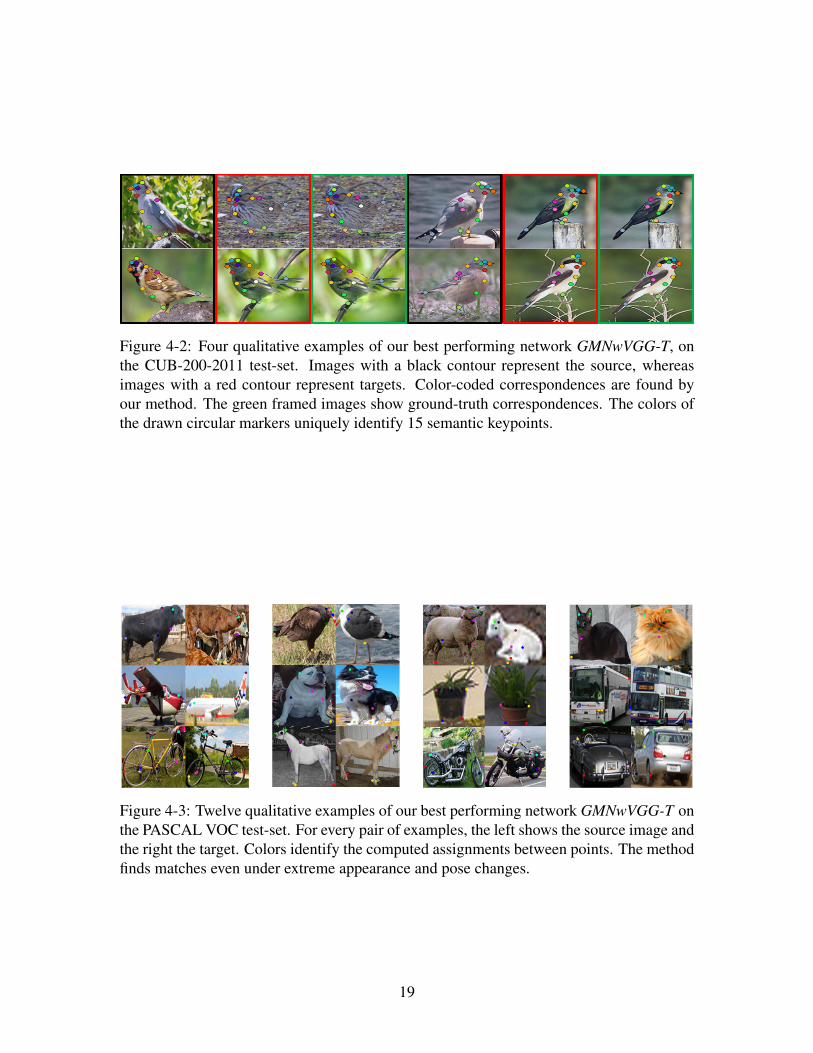
Figure 4-2: Four qualitative examples of our best performing network GMNwVGG-T, onthe CUB-200-2011 test-set. Images with a black contour represent the source, whereasimages with a red contour represent targets. Color-coded correspondences are found byour method. The green framed images show ground-truth correspondences. The colors ofthe drawn circular markers uniquely identify 15 semantic keypoints.

Figure 4-3: Twelve qualitative examples of our best performing network GMNwVGG-T onthe PASCAL VOC test-set. For every pair of examples, the left shows the source image andthe right the target. Colors identify the computed assignments between points. The methodfinds matches even under extreme appearance and pose changes.

19

20

Bibliography

[1] A. Berg, T. Berg, and J. Malik. Shape matching and object recognition using low dis-tortion correspondences. In Proceedings of Computer Vision and Pattern Recognition,2005.

[2] T. Brox, C. Bregler, and J. Malik. Large displacement optical flow. In Proceedings ofComputer Vision and Pattern Recognition, 2009.

[3] T. Brox and J. Malik. Large displacement optical flow: descriptor matching in varia-tional motion estimation. IEEE Transactions on Pattern Analysis and Machine Intel-ligence, 33(3):500–513, 2011.

[4] O. Duchenne, F. Bach, I. Kweon, and J. Ponce. A tensor-based algorithm for high-order graph matching. In Proceedings of Computer Vision and Pattern Recognition,2009.

[5] B. K. P. Horn and B. G. Schunck. Determining optical flow. Artificial Intelligence,17(1-3), 1981.

[6] Catalin Ionescu, Orestis Vantzos, and Cristian Sminchisescu. Training deep networkswith structured layers by matrix backpropagation. arXiv preprint arXiv:1509.07838,2015.

[7] M. Leordeanu, A. Zanfir, and C. Sminchisescu. Semi-supervised learning and opti-mization for hypergraph matching. In ICCV, 2011.

[8] C. Liu, J. Yuen, and A. Torralba. Sift flow: Dense correspondence across scenes andits applications. IEEE Transactions on Pattern Analysis and Machine Intelligence,33(5):978–994, 2011.

[9] Julian Quiroga, Thomas Brox, Frederic Devernay, and James Crowley. Dense semi-rigid scene flow estimation from rgbd images. In Computer Vision–ECCV 2014, pages567–582. Springer, 2014.

[10] Jerome Revaud, Philippe Weinzaepfel, Zaid Harchaoui, and Cordelia Schmid.Epicflow: Edge-preserving interpolation of correspondences for optical flow. In Pro-ceedings of the IEEE Conference on Computer Vision and Pattern Recognition, 2015.

[11] Karen Simonyan and Andrew Zisserman. Very deep convolutional networks for large-scale image recognition. arXiv preprint arXiv:1409.1556, 2014.

21

[12] D. Sun, S. Roth, and M.J. Black. Secrets of optical flow estimation and their princi-ples. In Proceedings of Computer Vision and Pattern Recognition, 2010.

[13] M. Werlberger, W. Trobin, T. Pock, A. Wedel, D. Cremers, and H. Bischof.Anisotropic huber-l1 optical flow. In British Machine Vision Conference, 2009.

[14] L. Xu, Jiaya Jia, and Yasuyuki Matsushita. Motion detail preserving optical flow es-timation. IEEE Transactions on Pattern Analysis and Machine Intelligence (TPAMI),34(9), 2012.

[15] Feng Zhou and Fernando De la Torre. Factorized graph matching. In Computer Visionand Pattern Recognition (CVPR), 2012 IEEE Conference on, pages 127–134. IEEE,2012.

22