Economic Growth and Development

Chapter 2

Principles and Concepts

2

After completing this chapter, you will be able to

1.Understand the difference between economic development and economic growth

2.Understand what are the determinants of economic growth.3.Understand the Neoclassical Solow growth model and

the endogenous growth model.4.Understand the determinants of growth as explained by

the empirical evidence.

3

• Economic growth is a measures only growth in economic

production. It is normally the %Δ of current real GDP and the

previous year real GDP.

• Economic development measures overall improvements in living

standards and in the quality of life. It cannot take place without

economic growth.

• What are the determinants of economic growth?

• Why are some countries rich and others poor?

• Capital accumulation only explains part of the differences in

economic growth across countries.

• Recently, economist have been paying special attention to

the role of determinants like geography and institutions.

i. The difference between Growth and development

4

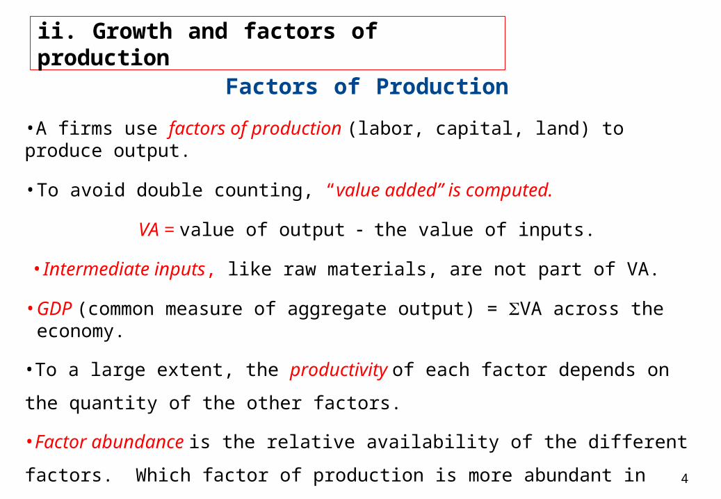
Factors of Production•A firms use factors of production (labor, capital, land) to produce output.

•To avoid double counting, “value added” is computed.

VA = value of output the value of inputs.

•Intermediate inputs, like raw materials, are not part of VA.

•GDP (common measure of aggregate output) = VA across the economy.

•To a large extent, the productivity of each factor depends on the

quantity of the other factors.

•Factor abundance is the relative availability of the different factors. Which factor of production is more abundant in developed economies? In

developing economies?

ii. Growth and factors of production

5

The Production Function• The production function is an equation of the joint effect of

the factors of production on output:Yt = F(Kt , Yt)

• The Cobb-Douglas production function:(1)

(2) 0 1

α 1 αt tY t A t K L

Kt is the stock of capital at year t, Lt the amount of labor and Yt output (e.g.,

GDP). At is a scale factor that links units of labor and capital to Y.

• This production function exhibits constant returns to scale. (e.g., if we time

each factor of production by a number, output is also timed by that number).

• Increasing/decreasing returns of scale: If labor and capital are multiplied by x,

then output is multiplied by more/less than x.

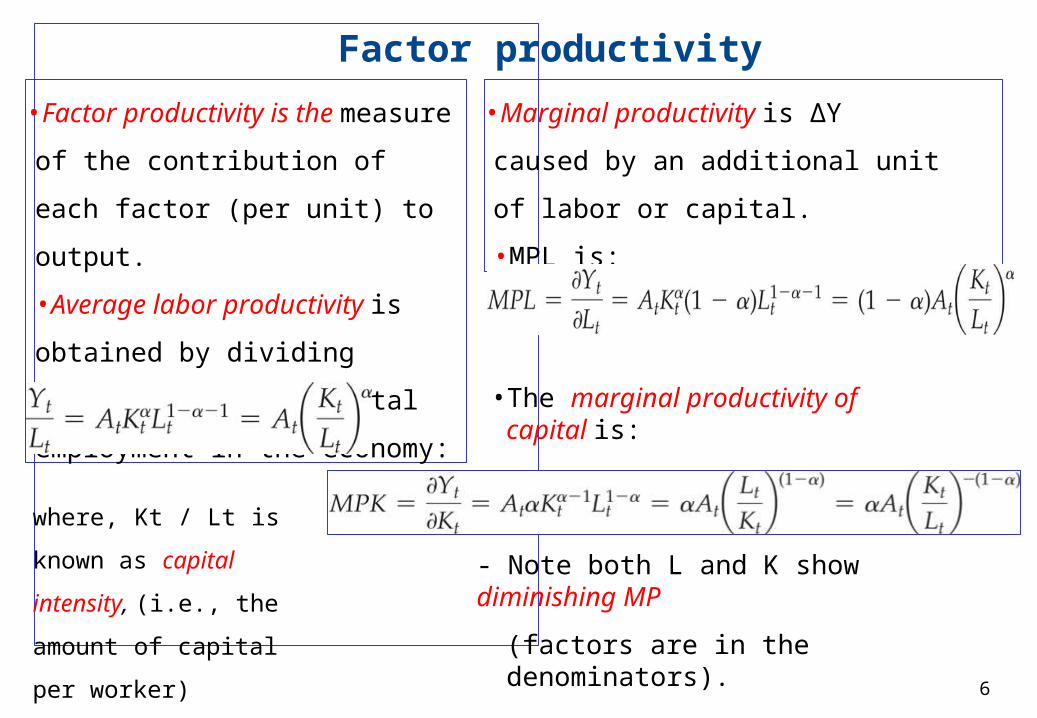
•Factor productivity is the measure of

the contribution of each factor (per

unit) to output.

•Average labor productivity is obtained

by dividing national output by total

employment in the economy:

where, Kt / Lt is known

as capital intensity, (i.e.,

the amount of capital per

worker)

Factor productivity•Marginal productivity is ΔY caused by an

additional unit of labor or capital.

• MPL is:

• The marginal productivity of capital is:

- Note both L and K show diminishing MP

(factors are in the denominators).6

•Factor shares are the proportions of national income used to pay for the capital and labor

in production.

•In theory, in a competitive economy a factor is paid its marginal productivity. Labor will

be added as long as the MPL exceeds the wage rate. Capital will be added as long as the

MPK is higher than the opportunity cost of capital, the IR.

• Thus, MPL = W and MPK = r.

•A useful result from the Cobb-Douglas production function is that, in equilibrium, the

factor shares are:

M P K .K t

Y t

M P L . L t

7

(1 )tY

Factor Shares

In advance economies the share of capital is about 1/3 of total income while the share of labor is

approximately 2/3.

• In the Cobb Douglas function, replace At with eat to assume that At growth at

constant rate a over time:

• Take logs of both sides:

• Differentiate wrt time to obtain growth rates:

Growth Accounting• Growth accounting estimates %ΔY that can be explained using the growth rate of the

labor force, the growth rate of the capital stock, and residual factors.

8

gy = a + αgK + (1-α) gL

• Growth in national output is decomposed

among:

1. the growth rate of capital multiplied by weight

(factor share) α2. the growth rate of labor multiplied by weight

(1-α)

3. Parameter a, the growth rate of total factor

productivity (TFP)

• Example: China between 2000 and 2005 where

average gy = 9.5,

α =.5, gK = 12.6, and gL = 1.0. Then, TFP:

a = 9.5 – (.5 * 12.6) – (.5 * 1) = 2.7

•TFP is defined as the part of an

economy’s growth rate that cannot be

explained with the growth of labor

and capital stock.

•TFP is often associated with

technological progress, but may also

be due to other things, such as

institutional reforms.

•TFP usually explains a big share of an

economy’s growth rate, and is the

biggest source of variation for cross-

country growth differences.

9

10

iii. The neo-classical Solow growth model

•“Neoclassical” growth model assumes competitive markets and a diminishing marginal

product of capital.

•Links production function with savings, investment, population growth, and technical

change

• Divide both sides of Cobb Douglas function by Lt :

Yt/Lt = A Ktα Lt

(1-α-1) = A (Kt / Lt )α

or, if yt =Yt/Lt and kt = Kt / Lt the above is expressed:

yt = A kt α

Labor productivity increases with capital intensity, or, in other words, at a given labor force

income per capita increases with capital accumulation.

The neo-classical Solow growth model

11

•Output per capita yt is

expressed as a function of

capital intensity (capital

per worker).

•The slope Yt ⁄ kt is the

average productivity of

capital. It decreases as

capital intensity increases,

meaning that average

capital productivity

decreases as capital

intensity increases.

• Capital intensity = K/L

• Average productivity of capital

= yt ⁄ kt

12

• National Income is allocated between consumption and saving:Yt = Ct + St

• Define savings rate (s) where:St = s Yt

• Capital stock increases through capital investment (assuming δ isdepreciation rate):

It = Kt+1 – Kt + δ Kt

• Assume closed economy (no trade) and no government, then:Yt = Ct + It so It = St

(From equations above)

• When an economy is in macroeconomic equilibrium, thenSt = sYt = It = Kt+1 – Kt +δKt

• Rearranging terms to find capital accumulation:Kt+1 = (1-δ) Kt + sYt

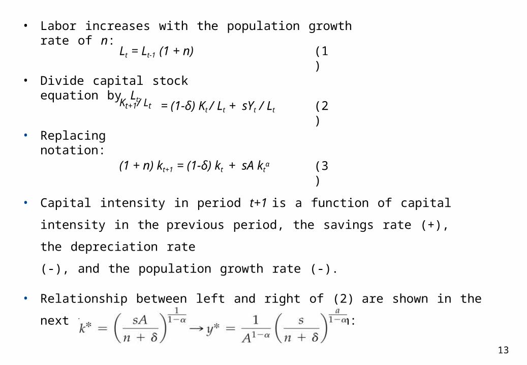
• Labor increases with the population growth rate of n:Lt = Lt-1 (1 + n) (1)

• Divide capital stock equation by Lt: Kt+1/ Lt = (1-δ) Kt / Lt + sYt / Lt (2)

• Replacing notation:

(1 + n) kt+1 = (1-δ) kt + sA ktα (3)

• Capital intensity in period t+1 is a function of capital intensity in

the previous period, the savings rate (+), the depreciation rate(-), and the population growth rate (-).

• Relationship between left and right of (2) are shown in the next figure

and by the “steady state” equation:()

13

Steady State in the Solow Model.

14

15

The Steady State in the Solow Growth Model

•At given rate of savings, population growth, and depreciation, the steady

state is reached where the growth of capital intensity and productivity

(income per capita) is zero.

• Transition growth paths:

If (1 + n) kt+1 > (1-δ) kt + sA ktα capital intensity falls, capital is “diluted”

because I (S) cannot overcome population growth and depreciation.

If (1 + n) kt+1 < (1-δ) kt + sA ktα capital intensity rises because I is high

enough to overcome population growth and depreciation.

• The production function assumes diminishing marginal product of capital. Assuming similar functions, therefore, poor countries that start out with

lower capital intensity have the potential to grow faster than rich

countries.

16

Technological Progress and the Steady State• What drives per capita growth in the steady state?

• Figure of next slide: An increase in TFP from A1 to A2 (represented by

an upward shift in the production function) acts to increase

capital intensity, and, therefore, output per person.•Absent new TFP shocks, the economy will settle into a new steady

state at k*2•In the Solow Model, these positive shocks to TFP are usually thought of as exogenous.

•The possibility of new technology diffusion increases the growth

potential of developing economies.

Technological Progress in the Solow Model.

17

18

The Effect of Different Savings Rates

• An increase in the savings rate leads to an increase in per capita

output in the steady state.• Historically, many high-savings Asian countries also grew fast.High I-rates also encourage adoption of new technology.

• On the other hand, at the time, China, the Soviet Union, and other centrally-planned countries invested at a high rate, but growth

sputtered as government directed investment was often wasted.

•In general, economists agree that while high rate of savings

and investment is important, the efficiency of investment is just as important.

Differences in Human Capital•Human capital is the skills, talents, and knowledge embodied in people (i.e. education).

•Modifying the Solow Model to incorporate h, the level of human capital (average years of schooling for instance):

(1)

And the steady state income per capita increases:

(24)

•Differences in h can explain much cross-country variation in growth and development, and human capital is a better predictor than investment rates.

•However, education does not account for a large part of growth variation, and some

highly educated nations lag in development.

•Moreover, like most factors, the direction of causality between human capital and

economic growth is unclear.19

20

Income Convergence•The most important prediction of the Solow model is income convergence:

poor countries should catch-up in terms of income per capita to rich countries.•Assumes all else being equal (savings, depreciation, but especially similar production functions i.e., s)•A greater marginal product of capital (return) means that poor countries have

the potential to grow faster than rich countries.•There is not much evidence of this convergence in practice, results are mixed: some countries have successfully converged, others have drifted further behind.•Most variation appears to be embodied in TFP (technology development and

adoption) which is exogenous to the Solow Model. How can we

endogenously explain differences in technological change across countries?

21

iv. Endogenous growth theory

Endogenous growth theory suggests that growth is generated by

endogenous technical change resulting from innovation.Boundless Knowledge-Based Growth

• Assuming constant technological change, potential for growth can be

boundless prevailing even limits to resources.• Technology depends on knowledge, and the more knowledge there is in an

economy, the higher the growth rate.• Unlike human capital, human knowledge is not embodied in people but can be

transmitted across time and space.

• Technology and knowledge develop through incentives communicated

through the market and, sometimes, through government policy.• Knowledge can spillover, grow and accumulate indefinitely. It is only

constrained by the number of people producing it.

22

Knowledge as a Non-Rival Good

•Knowledge non-rival good and can be consumed by the seller even after it is sold. It

is also an excludable good. A seller can exclude others from its consumption.

•Enforced property rights (such as patents and copyrights), for example, prevent access

to knowledge. Such exclusions can be important because people and firms need to have

an incentives (monopoly rents) to invest in research and development.

•Imperfect competition is necessary to encourage growth. (Recall that the Solow model

assumes perfect competition). However, a balance must be held between granting

temporary monopoly rights and promoting competition over the long run.

Basic Equations of the Romer Model Labor is divided between the productive sector (Y) and the research sector (A):

Lt = LYt + LAt

(1)

where human capital is the stock of knowledge at time t (At) times productive laborLyt at time t.

• The production function: (2)

• Since knowledge (At) depends on the allocation of labor to research, it isendogenous to the model and can vary over time.

• The increment of knowledge is given by the stock of knowledge multiplied by

the labor force in the research sector and a parameter that can represent, say, the efficiency of research:

23

24

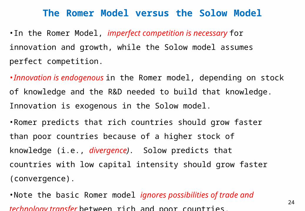
The Romer Model versus the Solow Model

•In the Romer Model, imperfect competition is necessary for

innovation and growth, while the Solow model assumes perfect

competition.

•Innovation is endogenous in the Romer model, depending on stock of knowledge and the R&D needed to build that knowledge. Innovation is

exogenous in the Solow model.

•Romer predicts that rich countries should grow faster than poor

countries because of a higher stock of knowledge (i.e., divergence). Solow predicts that countries with low capital intensity should

grow faster (convergence).

•Note the basic Romer model ignores possibilities of trade and

technology transfer between rich and poor countries.

•Are the protection of intellectual property rights (IPR) beneficial for poor countries?

25

v. Empirical analysis of economic growth

What drives the main differences in economic growth

between rich and poor countries?•Output per worker (labor productivity) is highly correlated with long-term growth.

•Table below: in 1988 Canada’s productivity was about 94% of the U.S. level. The capital-output ratio (K/Y) and TFP (A) level were about the same between

the countries. Most of the difference is explained by lower human capital ratio

(H/L) in Canada.

• The same is generally true with West European economies.

•Between the developed and developing economies differences in TFP

seems to be the main factor. What drives this difference in TFP?

– Geography (Sachs) or Institutions (North)?

– The growing consensus is that countries with stronger institutions develop faster.

Decomposition of Productivity Differences (Ratios to the US).

26

27

• Two geographic factors influencing growth: distance from the equator andgeographical isolation

• Rich countries tend to be located in temperate zones, poor countries in the tropics:

tropical disease (malaria, sleeping sickness),

intense heat makes hard labor (farming, construction) difficult,

rainfall volatility affects agricultural productivity and flooding.

• Landlocked areas tend to be underdeveloped:

lower population density means less challenges and cooperation in using resources,

lack of access to trade and outside influences (e.g., high transportation cost).

• Societies in tropics have not always been poor (e.g., Egypt, Aztecs, Inca, etc.)

Acemoglu, Johnson, and Robinson found negative correlation between urbanization

in 1500 (proxy for development) and income per capita now.

Log GDP per capita in 1995 among former European colonies and urbanization rate in 1500.

28

29

•Douglass North wrote (modern) important analysis arguing that institutions are key to

understanding why some countries developed earlier than others.

•Since then, much empirical analysis has shown a strong causal link from institutional

quality to long term growth. Another paper by Acemoglu, shows that protection from

expropriation risk enhances growth.

•Used instrumental variable technique to establish causation. Extractive or predatory

institutions established where settler mortality was high (e.g., Peru, Mexico, Congo,

etc.) while more efficient institutions established where settler mortality was low (e.g.,

North America, New Zealand, etc.).

•Most of the current research in development economies tries to understand the role of

institutions and their effects.

Average Protection against Risk of Expropriation and Log GDP Per Capita.

30

A negative correlation between settler mortality and protection against expropriation.

31

32