Decision Theory and the Normal Distribution -...

M3-1

1. Understand how the normal curve can be used inperforming break-even analysis.

2. Compute the expected value of perfect informationusing the normal curve.

3. Perform marginal analysis where products have aconstant marginal profit and loss.

After completing this module, students will be able to:

3

LEARNING OBJECTIVE

Decision Theory and theNormal Distribution

MODULE

MODULE OUTLINE

M3.1 Introduction

M3.2 Break-Even Analysis and the Normal Distribution

M3.3 Expected Value of Perfect Information and theNormal Distribution

Summary • Glossary • Key Equations • Solved Problems • Self-Test • Discussion Questions and

Problems • Bibliography

Appendix M3.1: Derivation of the Break-Even Point

Appendix M3.2: Unit Normal Loss Integral

Z00_REND1011_11_SE_MOD3 PP2.QXD 2/19/11 1:28 PM Page M3-1

M3.1 Introduction

In Chapter 3 in your text we look at examples that deal with only a small number of states ofnature and decision alternatives. But what if there were 50, 100, or even thousands of statesand/or alternatives? If you used a decision tree or decision table, solving the problem would bevirtually impossible. This module shows how decision theory can be extended to handleproblems of such magnitude.

We begin with the case of a firm facing two decision alternatives under conditions of nu-merous states of nature. The normal probability distribution, which is widely applicable in busi-ness decision making, is first used to describe the states of nature.

The normal distribution can beused when there are a largenumber of states and/oralternatives.

M3.2 Break-Even Analysis and the Normal Distribution

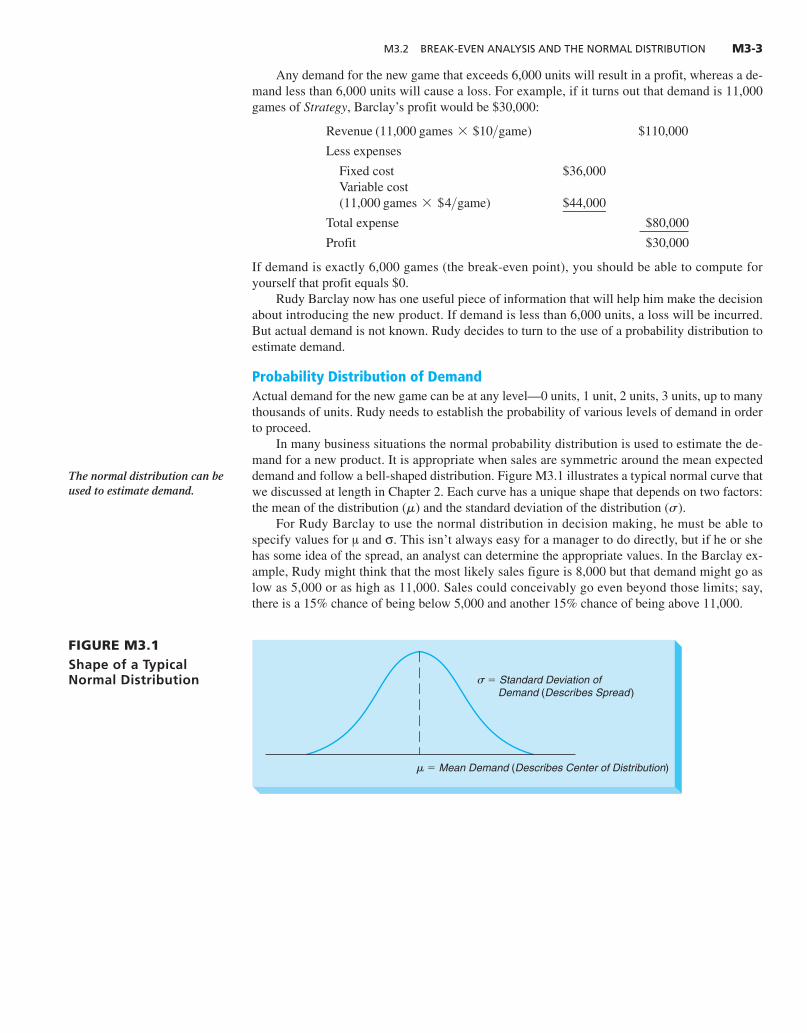
Break-even analysis, often called cost-volume analysis, answers several common managementquestions relating the effect of a decision to overall revenues or costs. At what point will webreak even, or when will revenues equal costs? At a certain sales volume or demand level, whatrevenues will be generated? If we add a new product line, will this action increase revenues? Inthis section we look at the basic concepts of break-even analysis and explore how the normalprobability distribution can be used in the decision making process.

Barclay Brothers Company’s New Product DecisionBarclay Brothers Company is a large manufacturer of adult parlor games. Its marketing vicepresident, Rudy Barclay, must make the decision whether to introduce a new game calledStrategy into the competitive market. Naturally, the company is concerned with costs, potentialdemand, and profit it can expect to make if it markets Strategy.

Rudy identifies the following relevant costs:

Fixed cost ( f ) $36,000 (costs that do not vary with volume produced, such asnew equipment, insurance, rent, and so on)

Variable cost (v) per (costs that are proportional to the number of gamesGame produced $4 produced, such as materials and labor)

The selling price(s) per unit is set at $10.The break-even point is the number of games at which total revenues are equal to total costs.

It can be expressed as follows:1

(M3-1)

So in Barclay’s case,

= 6,000 games of Strategy

Break-even point (games) =

$36,000

$10 - $4=

$36,000

$6

Break-even point (units) =

Fixed cost

Price>unit - Variable cost>unit=

f

s - v

=

=

M3-2 MODULE 3 • DECISION THEORY AND THE NORMAL DISTRIBUTION

1For a detailed explanation of the break-even equation, see Appendix M3.1 at the end of this module.


M3.2 BREAK-EVEN ANALYSIS AND THE NORMAL DISTRIBUTION M3-3

Any demand for the new game that exceeds 6,000 units will result in a profit, whereas a de-mand less than 6,000 units will cause a loss. For example, if it turns out that demand is 11,000games of Strategy, Barclay’s profit would be $30,000:

The normal distribution can beused to estimate demand.

� � Standard Deviation of Demand (Describes Spread )

� � Mean Demand (Describes Center of Distribution)

FIGURE M3.1Shape of a TypicalNormal Distribution

$110,000

Less expenses

Fixed cost $36,000Variable cost

$44,000

Total expense $80,000

Profit $30,000

(11,000 games * $4>game)

Revenue (11,000 games * $10>game)

If demand is exactly 6,000 games (the break-even point), you should be able to compute foryourself that profit equals $0.

Rudy Barclay now has one useful piece of information that will help him make the decisionabout introducing the new product. If demand is less than 6,000 units, a loss will be incurred.But actual demand is not known. Rudy decides to turn to the use of a probability distribution toestimate demand.

Probability Distribution of DemandActual demand for the new game can be at any level—0 units, 1 unit, 2 units, 3 units, up to manythousands of units. Rudy needs to establish the probability of various levels of demand in orderto proceed.

In many business situations the normal probability distribution is used to estimate the de-mand for a new product. It is appropriate when sales are symmetric around the mean expecteddemand and follow a bell-shaped distribution. Figure M3.1 illustrates a typical normal curve thatwe discussed at length in Chapter 2. Each curve has a unique shape that depends on two factors:the mean of the distribution ( ) and the standard deviation of the distribution ( ).

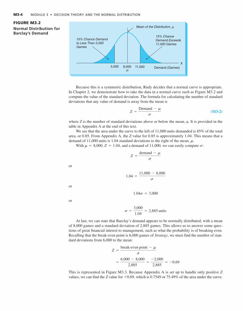
For Rudy Barclay to use the normal distribution in decision making, he must be able tospecify values for µ and σ. This isn’t always easy for a manager to do directly, but if he or shehas some idea of the spread, an analyst can determine the appropriate values. In the Barclay ex-ample, Rudy might think that the most likely sales figure is 8,000 but that demand might go aslow as 5,000 or as high as 11,000. Sales could conceivably go even beyond those limits; say,there is a 15% chance of being below 5,000 and another 15% chance of being above 11,000.

sm


�

Demand (Games)X

5,000 8,000 11,000

Mean of the Distribution, �

15% Chance DemandIs Less Than 5,000Games

15% Chance Demand Exceeds 11,000 Games

FIGURE M3.2Normal Distribution forBarclay’s Demand

Because this is a symmetric distribution, Rudy decides that a normal curve is appropriate.In Chapter 2, we demonstrate how to take the data in a normal curve such as Figure M3.2 andcompute the value of the standard deviation. The formula for calculating the number of standarddeviations that any value of demand is away from the mean is

(M3-2)

where Z is the number of standard deviations above or below the mean, µ. It is provided in thetable in Appendix A at the end of this text.

We see that the area under the curve to the left of 11,000 units demanded is 85% of the totalarea, or 0.85. From Appendix A, the Z value for 0.85 is approximately 1.04. This means that ademand of 11,000 units is 1.04 standard deviations to the right of the mean, .

With and a demand of 11,000, we can easily compute :

or

or

or

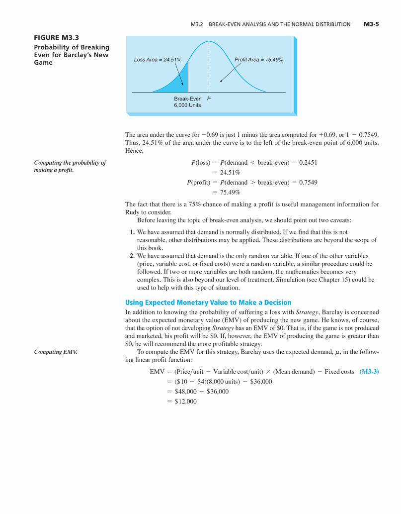
At last, we can state that Barclay’s demand appears to be normally distributed, with a meanof 8,000 games and a standard deviation of 2,885 games. This allows us to answer some ques-tions of great financial interest to management, such as what the probability is of breaking even.Recalling that the break-even point is 6,000 games of Strategy, we must find the number of stan-dard deviations from 6,000 to the mean:

This is represented in Figure M3.3. Because Appendix A is set up to handle only positive Zvalues, we can find the Z value for which is 0.7549 or 75.49% of the area under the curve.+0.69,

=

6,000 - 8,000

2,885=

-2,000

2,885= -0.69

Z =

break-even point - m

s

s =

3,000

1.04= 2,885 units

1.04s = 3,000

1.04 =

11,000 - 8,000

s

Z =

demand - m

s

sm = 8,000, Z = 1.04,m

Z =

Demand - m

s



Break-Even6,000 Units

Profit Area = 75.49%Loss Area = 24.51%

�

FIGURE M3.3Probability of BreakingEven for Barclay’s NewGame

M3.2 BREAK-EVEN ANALYSIS AND THE NORMAL DISTRIBUTION M3-5

Computing the probability ofmaking a profit.

The area under the curve for is just 1 minus the area computed for or Thus, 24.51% of the area under the curve is to the left of the break-even point of 6,000 units.Hence,

The fact that there is a 75% chance of making a profit is useful management information forRudy to consider.

Before leaving the topic of break-even analysis, we should point out two caveats:

1. We have assumed that demand is normally distributed. If we find that this is notreasonable, other distributions may be applied. These distributions are beyond the scope ofthis book.

2. We have assumed that demand is the only random variable. If one of the other variables(price, variable cost, or fixed costs) were a random variable, a similar procedure could befollowed. If two or more variables are both random, the mathematics becomes verycomplex. This is also beyond our level of treatment. Simulation (see Chapter 15) could beused to help with this type of situation.

Using Expected Monetary Value to Make a DecisionIn addition to knowing the probability of suffering a loss with Strategy, Barclay is concernedabout the expected monetary value (EMV) of producing the new game. He knows, of course,that the option of not developing Strategy has an EMV of $0. That is, if the game is not producedand marketed, his profit will be $0. If, however, the EMV of producing the game is greater than$0, he will recommend the more profitable strategy.

To compute the EMV for this strategy, Barclay uses the expected demand, , in the follow-ing linear profit function:

(M3-3)

= $12,000

= $48,000 - $36,000

= ($10 - $4)(8,000 units) - $36,000

EMV = (Price>unit - Variable cost>unit) * (Mean demand) - Fixed costs

m

= 75.49%

P(profit) = P(demand 7 break-even) = 0.7549

= 24.51%

P(loss) = P(demand 6 break-even) = 0.2451

1 - 0.7549.+0.69,-0.69

Computing EMV.



M3.3 Expected Value of Perfect Information and the Normal Distribution

Let’s return to the Barclay Brothers problem to see how to compute the expected value of per-fect information (EVPI) and expected opportunity loss (EOL) associated with introducing thenew game. The two steps follow:

Two Steps to Compute EVPI and EOL

1. Determine the opportunity loss function.2. Use the opportunity loss function and the unit normal loss integral (given in Appendix

M3.2 at the end of this module) to find EOL, which is the same as EVPI.

Opportunity Loss FunctionThe opportunity loss function describes the loss that would be suffered by making the wrong de-cision. We saw earlier that Rudy’s break-even point is 6,000 sets of the game Strategy. If Rudyproduces and markets the new game and sales are greater than 6,000 units, he has made the rightdecision; in this case there is no opportunity loss ($0). If, however, he introduces Strategy andsales are less than 6,000 games, he has selected the wrong alternative. The opportunity loss isjust the money lost if demand is less than the break-even point; for example, if demand is 5,999games, Barclay loses $6 (= $10 price/unit - $4 cost/unit). With a $6 loss for each unit of salesless than the break-even point, the total opportunity loss is $6 multiplied by the number of unitsunder 6,000. If only 5,000 games are sold, the opportunity loss will be 1,000 units less than thebreak-even point times $6 per unit = $6,000. For any level of sales, X, Barclay’s opportunity lossfunction can be expressed as follows:

In general, the opportunity loss function can be computed by

(M3-4)

where

loss per unit when sales are below the break-even point

sales in units

Expected Opportunity LossThe second step is to find the expected opportunity loss. This is the sum of the opportunitylosses multiplied by the appropriate probability values. But in Barclay’s case there are avery large number of possible sales values. If the break-even point is 6,000 games, therewill be 6,000 possible sales values, from 0, 1, 2, 3, up to 6,000 units. Thus, determining theEOL would require setting 6,000 probability values that correspond to the 6,000 possible

X =

K =

Opportunity loss = eK(break-even point - X) for X … break-even point

$0 for X 7 break-even point

Opportunity loss = e $6(6,000 - X) for X … 6,000 games

$0 for X 7 6,000 games

Rudy has two choices at this point. He can recommend that the firm proceed with the newgame; if so, he estimates there is a 75% chance of at least breaking even and an EMV of$12,000. Or, he might prefer to do further market research before making a decision. This bringsup the subject of the expected value of perfect information.


M3.3 EXPECTED VALUE OF PERFECT INFORMATION AND THE NORMAL DISTRIBUTION M3-7

sales values. These numbers would be multiplied and added together, a very lengthy andtedious task.

When we assume that there are an infinite (or very large) number of possible sales valuesthat follow a normal distribution, the calculations are much easier. Indeed, when the unit normalloss integral is used, EOL can be computed as follows:

(M3-5)

where

expected opportunity loss

loss per unit when sales are below the break-even point

standard deviation of the distribution

value for the unit normal loss integral in Appendix M3.2 for a given value of D

(M3-6)

where

absolute value sign

mean sales

Here is how Rudy can compute EOL for his situation:

Now refer to the unit normal loss integral table in Appendix M3.2. Look in the “0.6” row andread over to the “0.9” column. This is N(0.69), which is 0.1453:

Therefore,

Because EVPI and minimum EOL are equivalent, the EVPI is also $2,515.14. This is themaximum amount that Rudy should be willing to spend on additional marketing information.

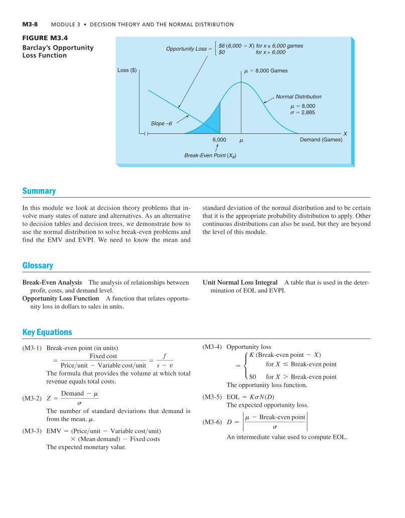
The relationship between the opportunity loss function and the normal distribution is shownin Figure M3.4. This graph shows both the opportunity loss and the normal distribution with amean of 8,000 games and a standard deviation of 2,885. To the right of the break-even point wenote that the loss function is 0. To the left of the break-even point, the opportunity loss functionincreases at a rate of $6 per unit, hence the slope of -6. The use of Appendix M3.2 and Equa-tion M3-5 allows us to multiply the $6 unit loss times each of the probabilities between 6,000units and 0 units and to sum these multiplications.

= ($6)(2,885)(0.1453) = $2,515.14

EOL = KsN(0.69)

N(0.69) = 0.1453

D = 2 8,000 - 6,000

2,8852 = 0.69 = 0.60 + 0.09

s = 2,885

K = $6

m =

ƒ ƒ =

D = 2 m - Break-even point

s2

N(D) =

s =

K =

EOL =

EOL = KsN(D)

Using the unit normal lossintegral.

EVPI and Minimum EOL areequivalent.



Key Equations

(M3-1) Break-even point (in units)

The formula that provides the volume at which totalrevenue equals total costs.

(M3-2)

The number of standard deviations that demand isfrom the mean,

(M3-3)

The expected monetary value.* (Mean demand) - Fixed costs

EMV = (Price>unit - Variable cost>unit)

m.

Z =

Demand - m

s

=

Fixed cost

Price>unit - Variable cost>unit=

f

s - v

(M3-4) Opportunity loss

The opportunity loss function.

(M3-5)The expected opportunity loss.

(M3-6)

An intermediate value used to compute EOL.


s2

EOL = KsN(D)

= c K (Break-even point - X)

for X … Break-even point

$0 for X 7 Break-even point

�6,000

Normal Distribution

Slope –6

Break-Even Point (XB)

Demand (Games)X

Loss ($)

Opportunity Loss �

� � 8,000 Games

$6 (6,000 – X ) for x ≤ 6,000 games$0 for x > 6,000 ⎧

⎨⎩

� � 8,000� � 2,885

FIGURE M3.4Barclay’s OpportunityLoss Function

Summary

In this module we look at decision theory problems that in-volve many states of nature and alternatives. As an alternativeto decision tables and decision trees, we demonstrate how touse the normal distribution to solve break-even problems andfind the EMV and EVPI. We need to know the mean and

standard deviation of the normal distribution and to be certainthat it is the appropriate probability distribution to apply. Othercontinuous distributions can also be used, but they are beyondthe level of this module.

Glossary

Break-Even Analysis The analysis of relationships betweenprofit, costs, and demand level.

Opportunity Loss Function A function that relates opportu-nity loss in dollars to sales in units.

Unit Normal Loss Integral A table that is used in the deter-mination of EOL and EVPI.


SOLVED PROBLEMS M3-9

Solved Problem M3-1Terry Wagner is considering self-publishing a book on yoga. She has been teaching yoga for more than20 years. She believes that the fixed costs of publishing the book will be about $10,000. The variablecosts are $5.50, and the price of the yoga book to bookstores is expected to be $12.50. What is thebreak-even point for Terry?

SolutionThis problem can be solved using the break-even formulas in the module, as follows:

Solved Problem M3-2The annual demand for a new electric product is expected to be normally distributed with a mean of16,000 and a standard deviation of 2,000. The break-even point is 14,000 units. For each unit less than14,000, the company will lose $24. Find the expected opportunity loss.

SolutionThe expected opportunity loss (EOL) is

We are given the following:

Using Equation M3-6, we find

EOL = KsN(1) = 24(2,000)(0.08332) = $3,999.36

N(D) = N(1) = 0.08332 from Appendix M3.2


s2 = 2 16,000 - 14,000

2,0002 = 1

s = 2,000

m = 16,000

K = loss per unit = $24

EOL = KsN(D)

= 1,429 units

=

$10,000

$7

Break-even point in units =

$10,000

$12.50 - $5.50

Solved Problems



Self-Test

Discussion Questions and Problems

Discussion QuestionsM3-1 What is the purpose of conducting break-even analy-

sis?

M3-2 Under what circumstances can the normal distribu-tion be used in break-even analysis? What does itusually represent?

M3-3 What assumption do you have to make about the re-lationship between EMV and a state of nature whenyou are using the mean to determine the value ofEMV?

M3-4 Describe how EVPI can be determined when the dis-tribution of the states of nature follows a normal dis-tribution.

ProblemsM3-5 A publishing company is planning on developing an

advanced quantitative analysis book for graduatestudents in doctoral programs. The company esti-mates that sales will be normally distributed, withmean sales of 60,000 copies and a standard devia-tion of 10,000 books. The book will cost $16 to pro-duce and will sell for $24; fixed costs will be$160,000.

(a) What is the company’s break-even point?(b) What is the EMV?

M3-6 Refer to Problem M3-5.(a) What is the opportunity loss function?(b) Compute the expected opportunity loss.(c) What is the EVPI?(d) What is the probability that the new book will be

profitable?(e) What do you recommend that the firm do?

M3-7 Barclay Brothers Company, the firm discussed inthis module, thinks it underestimated the mean forits game Strategy. Rudy Barclay thinks expectedsales may be 9,000 games. He also thinks that thereis a 20% chance that sales will be less than 6,000games and a 20% chance that he can sell more than12,000 games.(a) What is the new standard deviation of demand?(b) What is the probability that the firm will incur a

loss?(c) What is the EMV?(d) How much should Rudy be willing to pay now

for a market research study?

� Before taking the self-test, refer back to the learning objectives at the beginning of the module and the glossary at the end ofthe module.

� Use the key at the back of the book to correct your answers.� Restudy pages that correspond to any questions that you answered incorrectly or material you feel uncertain about.

5. The minimum EOL is equal to thea. break-even point.b. EVPI.c. maximum EMV.d. Z value for the break-even point.

6. Which of the following would indicate the maximum thatshould be paid for any additional information?a. the break-even pointb. the EVPIc. the EMV of the meand. total fixed cost

7. The opportunity loss function is expressed as a functionof the demand (X) when the break-even point and the lossper unit (K) are known. Which of the following is true ofthe opportunity loss?a. Opportunity loss K (Break-even point - X) for X

Break-even pointb. Opportunity loss K (X - Break-even point) for X

Break-even pointc. Opportunity loss K (Break-even point - X) for

X Break-even pointd. Opportunity loss K (X - Break-even point) for

X Break-even point6

=

6

=

Ú=

Ú=

1. Another name for break-even analysis isa. normal analysis.b. variable-cost analysis.c. cost-volume analysis.d. standard analysis.e. probability analysis.

2. The break-even point is the quantity at whicha. total variable cost equals total fixed cost.b. total revenue equals total variable cost.c. total revenue equals total fixed cost.d. total revenue equals total cost.

3. If demand is greater than the break-even point,a. profit will equal zero.b. profit will be greater than zero.c. profit will be negative.d. total fixed cost will equal total variable cost.

4. If the break-even point is less than the mean, the Z valuewilla. be negative.b. equal zero.c. be positive.d. be impossible to calculate.


DISCUSSION QUESTIONS AND PROBLEMS M3-11

M3-8 True-Lens, Inc., is considering producing long-wearing contact lenses. Fixed costs will be $24,000,with a variable cost per set of lenses of $8. Thelenses will sell to optometrists for $24 per set.(a) What is the firm’s break-even point?(b) If expected sales are 2,000 sets, what should

True-Lens do, and what are the expected profits?

M3-9 Leisure Supplies produces sinks and ranges fortravel trailers and recreational vehicles. The unitprice on its double sink is $28 and the unit cost is$20. The fixed cost in producing the double sink is$16,000. Mean sales for the double sinks have been35,000 units, and the standard deviation has beenestimated to be 8,000 sinks. Determine the ex-pected monetary value for these sinks. If the stan-dard deviation were actually 16,000 units insteadof 8,000 units, what effect would this have on theexpected monetary value?

M3-10 Belt Office Supplies sells desks, lamps, chairs, andother related supplies. The company’s executivelamp sells for $45, and Elizabeth Belt has deter-mined that the break-even point for executivelamps is 30 lamps per year. If Elizabeth does notmake the break-even point, she loses $10 per lamp.The mean sales for executive lamps has been 45,and the standard deviation is 30.(a) Determine the opportunity loss function.(b) Determine the expected opportunity loss.(c) What is the EVPI?

M3-11 Elizabeth Belt is not completely certain that theloss per lamp is $10 if sales are below the break-even point (refer to Problem M3-10). The loss perlamp could be as low as $8 or as high as $15. Whateffect would these two values have on the expectedopportunity loss?

M3-12 Leisure Supplies is considering the possibility ofusing a new process for producing sinks. This newprocess would increase the fixed cost by $16,000.In other words, the fixed cost would double (seeProblem M3-9). This new process will improve thequality of the sinks and reduce the cost it takes toproduce each sink. It will cost only $19 to producethe sinks using the new process.(a) What do you recommend?(b) Leisure Supplies is considering the possibility

of increasing the purchase price to $32 usingthe old process given in Problem M3-9. It is ex-pected that this will lower the mean sales to26,000 units. Should Leisure Supplies increasethe selling price?

M3-13 Quality Cleaners specializes in cleaning apartmentunits and office buildings. Although the work is nottoo enjoyable, Joe Boyett has been able to realize aconsiderable profit in the Chicago area. Joe is nowthinking about opening another Quality Cleaners inMilwaukee. To break even, Joe would need to get

200 cleaning jobs per year. For every job under200, Joe will lose $80. Joe estimates that the aver-age sales in Milwaukee are 350 jobs per year, witha standard deviation of 150 jobs. A market researchteam has approached Joe with a proposition to per-form a marketing study on the potential for hiscleaning business in Milwaukee. What is the mostthat Joe would be willing to pay for the market re-search?

M3-14 Diane Kennedy is contemplating the possibility ofgoing into competition with Primary Pumps, amanufacturer of industrial water pumps. Diane hasgathered some interesting information from afriend of hers who works for Primary. Diane hasbeen told that the mean sales for Primary are 5,000units and the standard deviation is 50 units. Theopportunity loss per pump is $100. Furthermore,Diane has been told that the most that Primary iswilling to spend for market research for the de-mand potential for pumps is $500. Diane is inter-ested in knowing the break-even point for PrimaryPumps. Given this information, compute the break-even point.

M3-15 Jack Fuller estimates that the break-even point forEM5, a standard electrical motor, is 500 motors.For any motor that is not sold, there is an opportu-nity loss of $15. The average sales have been 700motors, and 20% of the time sales have been be-tween 650 and 750 motors. Jack has just been ap-proached by Radner Research, a firm thatspecializes in performing marketing studies for in-dustrial products, to perform a standard marketingstudy. What is the most that Jack would be willingto pay for market research?

M3-16 Jack Fuller believes that he has made a mistake inhis sales figures for EM5 (see Problem M3-15 fordetails). He believes that the average sales are 750instead of 700 units. Furthermore, he estimates that20% of the time, sales will be between 700 and 800units. What effect will these changes have on yourestimate of the amount that Jack should be willingto pay for market research?

M3-17 Patrick’s Pressure Wash pays $4,000 per month tolease equipment that it uses for washing sidewalks,swimming pool decks, houses, and other things.Based on the size of a work crew, the cost of the la-bor used on a typical job is $80 per job. However,Patrick charges $120 per job, which results in aprofit of $40 per job. How many jobs would beneeded to break even each month?

M3-18 Determine the EVPI for Patrick’s Pressure Wash inProblem M3-17 if the average monthly demand is120 jobs, with a standard deviation of 15.

M3-19 If Patrick (see Problem M3-17) charged $150 perjob while his labor cost remained at $80 per job,what would be the break-even point?



Bibliography

Drenzer, Z., and G. O. Wesolowsky. “The Expected Value of Perfect Informa-tion in Facility Location,” Operations Research (March–April 1980):395–402.

Hammond, J. S., R. L. Kenney, and H. Raiffa. “The Hidden Traps inDecision Making,” Harvard Business Review (September–October1998): 47–60.

Keaton, M. “A New Functional Approximation to the Standard NormalLoss Integral,” Inventory Management Journal (Second Quarter1994): 58–62.

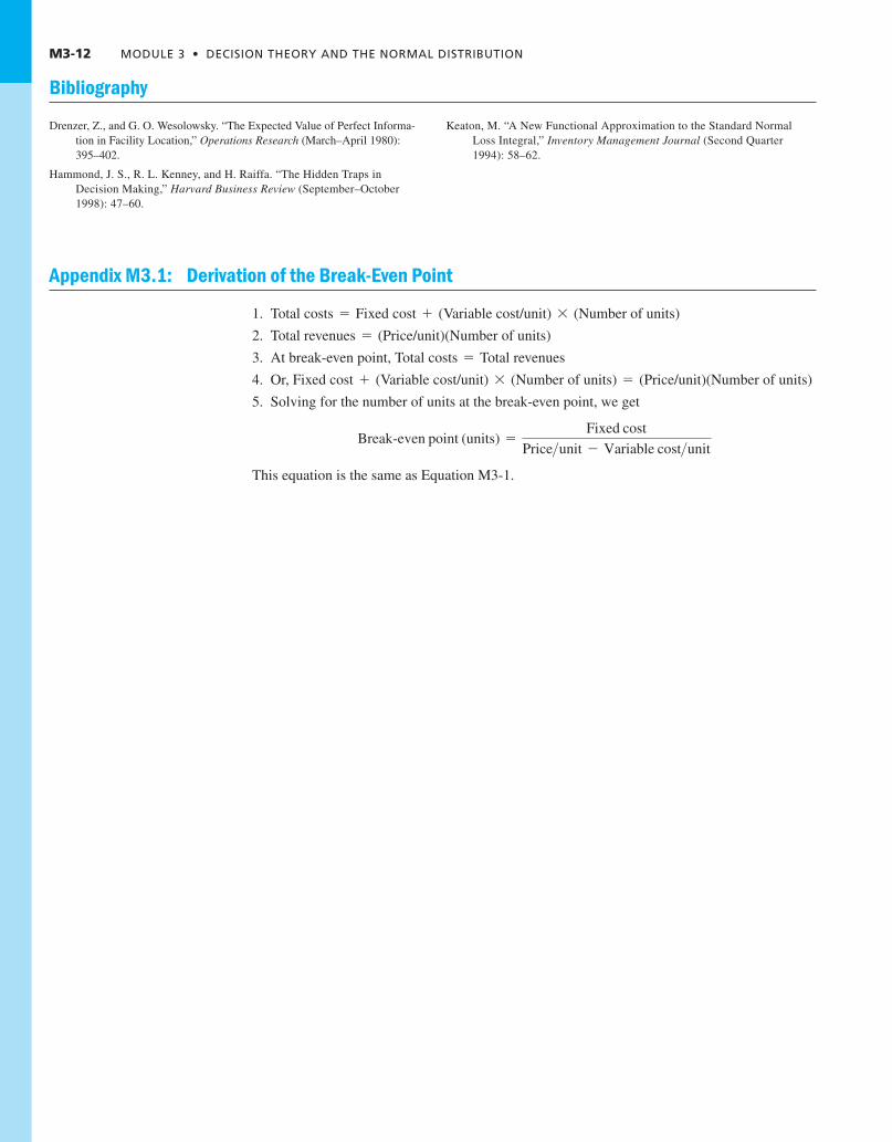
Appendix M3.1: Derivation of the Break-Even Point

1. Total costs Fixed cost (Variable cost/unit) (Number of units)

2. Total revenues (Price/unit)(Number of units)

3. At break-even point, Total costs Total revenues

4. Or, Fixed cost (Variable cost/unit) (Number of units) (Price/unit)(Number of units)

5. Solving for the number of units at the break-even point, we get

This equation is the same as Equation M3-1.

Break-even point (units) =

Fixed cost

Price>unit - Variable cost>unit

=*+

=

=

*+=


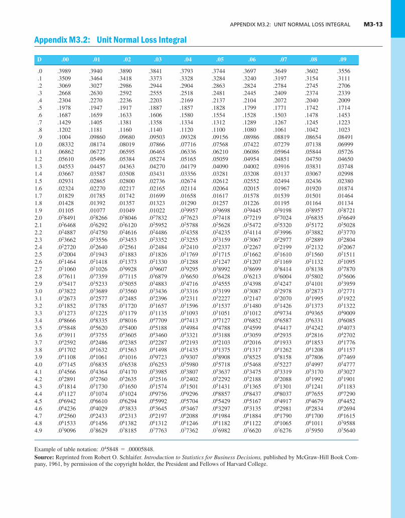
APPENDIX M3.2: UNIT NORMAL LOSS INTEGRAL M3-13

Appendix M3.2: Unit Normal Loss Integral

D .00 .01 .02 .03 .04 .05 .06 .07 .08 .09

.0 .3989 .3940 .3890 .3841 .3793 .3744 .3697 .3649 .3602 .3556

.1 .3509 .3464 .3418 .3373 .3328 .3284 .3240 .3197 .3154 .3111

.2 .3069 .3027 .2986 .2944 .2904 .2863 .2824 .2784 .2745 .2706

.3 .2668 .2630 .2592 .2555 .2518 .2481 .2445 .2409 .2374 .2339

.4 .2304 .2270 .2236 .2203 .2169 .2137 .2104 .2072 .2040 .2009

.5 .1978 .1947 .1917 .1887 .1857 .1828 .1799 .1771 .1742 .1714

.6 .1687 .1659 .1633 .1606 .1580 .1554 .1528 .1503 .1478 .1453

.7 .1429 .1405 .1381 .1358 .1334 .1312 .1289 .1267 .1245 .1223

.8 .1202 .1181 .1160 .1140 .1120 .1100 .1080 .1061 .1042 .1023

.9 .1004 .09860 .09680 .09503 .09328 .09156 .08986 .08819 .08654 .084911.0 .08332 .08174 .08019 .07866 .07716 .07568 .07422 .07279 .07138 .069991.1 .06862 .06727 .06595 .06465 .06336 .06210 .06086 .05964 .05844 .057261.2 .05610 .05496 .05384 .05274 .05165 .05059 .04954 .04851 .04750 .046501.3 .04553 .04457 .04363 .04270 .04179 .04090 .04002 .03916 .03831 .037481.4 .03667 .03587 .03508 .03431 .03356 .03281 .03208 .03137 .03067 .029981.5 .02931 .02865 .02800 .02736 .02674 .02612 .02552 .02494 .02436 .023801.6 .02324 .02270 .02217 .02165 .02114 .02064 .02015 .01967 .01920 .018741.7 .01829 .01785 .01742 .01699 .01658 .01617 .01578 .01539 .01501 .014641.8 .01428 .01392 .01357 .01323 .01290 .01257 .01226 .01195 .01164 .011341.9 .01105 .01077 .01049 .01022 .029957 .029698 .029445 .029198 .028957 .0287212.0 .028491 .028266 .028046 .027832 .027623 .027418 .027219 .027024 .026835 .0266492.1 .026468 .026292 .026120 .025952 .025788 .025628 .025472 .025320 .025172 .0250282.2 .024887 .024750 .024616 .024486 .024358 .024235 .024114 .023996 .023882 .0237702.3 .023662 .023556 .023453 .023352 .023255 .023159 .023067 .022977 .022889 .0228042.4 .022720 .022640 .022561 .022484 .022410 .022337 .022267 .022199 .022132 .0220672.5 .022004 .021943 .021883 .021826 .021769 .021715 .021662 .021610 .021560 .0215112.6 .021464 .021418 .021373 .021330 .021288 .021247 .021207 .021169 .021132 .0210952.7 .021060 .021026 .039928 .039607 .039295 .038992 .038699 .038414 .038138 .0378702.8 .037611 .037359 .037115 .036879 .036650 .036428 .036213 .036004 .035802 .0356062.9 .035417 .035233 .035055 .034883 .034716 .034555 .034398 .034247 .034101 .0339593.0 .033822 .033689 .033560 .033436 .033316 .033199 .033087 .032978 .032873 .0327713.1 .032673 .032577 .032485 .032396 .032311 .032227 .032147 .032070 .031995 .0319223.2 .031852 .031785 .031720 .031657 .031596 .031537 .031480 .031426 .031373 .0313223.3 .031273 .031225 .031179 .031135 .031093 .031051 .031012 .049734 .049365 .0490093.4 .048666 .048335 .048016 .047709 .047413 .047127 .046852 .046587 .046331 .0460853.5 .045848 .045620 .045400 .045188 .044984 .044788 .044599 .044417 .044242 .0440733.6 .043911 .043755 .043605 .043460 .043321 .043188 .043059 .042935 .042816 .0427023.7 .042592 .042486 .042385 .042287 .042193 .042103 .042016 .041933 .041853 .0417763.8 .041702 .041632 .041563 .041498 .041435 .041375 .041317 .041262 .041208 .0411573.9 .041108 .041061 .041016 .059723 .059307 .058908 .058525 .058158 .057806 .0574694.0 .057145 .056835 .056538 .056253 .055980 .055718 .055468 .055227 .054997 .0547774.1 .054566 .054364 .054170 .053985 .053807 .053637 .053475 .053319 .053170 .0530274.2 .052891 .052760 .052635 .052516 .052402 .052292 .052188 .052088 .051992 .0519014.3 .051814 .051730 .051650 .051574 .051501 .051431 .051365 .051301 .051241 .0511834.4 .051127 .051074 .051024 .069756 .069296 .068857 .068437 .068037 .067655 .0672904.5 .066942 .066610 .066294 .065992 .065704 .065429 .065167 .064917 .064679 .0644524.6 .064236 .064029 .063833 .063645 .063467 .063297 .063135 .062981 .062834 .0626944.7 .062560 .062433 .062313 .062197 .062088 .061984 .061884 .061790 .061700 .0616154.8 .061533 .061456 .061382 .061312 .061246 .061182 .061122 .061065 .061011 .0795884.9 .079096 .078629 .078185 .077763 .077362 .076982 .076620 .076276 .075950 .075640

Example of table notation: .045848 .00005848.Source: Reprinted from Robert O. Schlaifer. Introduction to Statistics for Business Decisions, published by McGraw-Hill Book Com-pany, 1961, by permission of the copyright holder, the President and Fellows of Harvard College.

=


Decision Theory and the Normal Distribution -...

Documents

Transcript of Decision Theory and the Normal Distribution -...