Decision-Making Using the Analytic Hierarchy Process (AHP) and

JMP® Scripting Language

Melvin Alexander, University of Maryland Medical Center, Baltimore, MD

ABSTRACT

JMP® scripting language (JSL) can be used to implement the Analytic Hierarchy Process (AHP). AHP helps decision-

makers choose the best solution from several options and selection criteria. Thomas Saaty developed AHP as a

decision-making method in the 1970s. AHP has broad applications in operations research, quality engineering, and

design-for-six-sigma (DFSS) situations. AHP builds a hierarchy (ranking) of decision items using comparisons

between each pair of items expressed as a matrix. Paired comparisons produce weighting scores that measure how

much importance items and criteria have with each other. This presentation will model AHP using personal, business,

and medical decision-making examples. JSL scripts will generate output that includes measures of criteria and

selection importance and data consistency.

INTRODUCTION

This presentation is about one of the most famous methods for making multi-criteria decisions called the Analytic

Hierarchy Process or AHP. AHP was developed to optimize decision making when one is faced with a mix of

qualitative, quantitative, and sometimes conflicting factors that are taken into consideration. AHP has been very

effective in making complicated, often irreversible decisions.

This presentation will show how JSL implements AHP to help decision makers choose the best solution among

several alternatives across multiple criteria. With JSL, I will build an AHP model using the example of choosing a

MDCT scanning device. I will describe some recent uses and present final notes.

Decision-making involves the use of intelligence, wisdom and creativity in order for humans to satisfy basic needs or

to survive. Evaluating a decision requires several considerations such as the benefits derived from making the right

decision, the costs, the risks, and losses resulting from the actions (or non-actions) taken if the wrong decision is

made.

Decision-making methods range from reliance on chance (such as flipping coins, reading tea leaves or tarot cards) to

the use of more structured decision-making tools. Sound decision-making involves weighing all the factors that are

important. Six sigma belts must carefully weigh the advantages and disadvantages of decision choices so that the

future success and survival in business or life can be optimized, nothing is guaranteed.

Modern Day decision-making has been inherently complex when many factors have to be weighed against competing

priorities. One of the modern tools developed in the last 30 years used to assess, prioritize, rank, and evaluate

decision choices is the Analytic Hierarchy Process (AHP) developed by Thomas Saaty [1-4].

Thomas Saaty developed AHP in the 1970s as a way of dealing with weapons tradeoffs, resource and asset

allocation, and decision making when he was a professor at the Wharton School of Business and a consultant with

the U.S. State Department’s Arms Control Disarmament Agency. There he was faced with the problem of dealing

with high costs and a host of considerations with many factors that conflicted with each other or were not easily

specified.

AHP takes the judgments of decision makers to form a decomposition of problems into hierarchies. Problem

complexity is represented by the number of levels in the hierarchy which combine with the decision-maker’s model of

the problem to be solved. The hierarchy is used to derive ratio-scaled measures for decision alternatives and

determines the relative value alternatives have against organizational goals (customer satisfaction, product/service,

financial, human resource, and organizational effectiveness) and project risks. AHP uses matrix algebra to sort out

factors to arrive at a mathematically optimal solution. AHP is a time-tested method that has been used in making

multi-billion dollar decisions.

AHP derives ratio scales from paired comparisons of factors and choice options.

Typical applications where AHP has been used are in:

Prioritizing factors and requirements that impact software development and productivity,

Choosing among several strategies for improving safety features in motor vehicles,

Estimating cost and scheduling options for material requirements planning (MRP),

Selecting desired software components from several software vendors,

Evaluating the quality of research and investment proposals.

AHP uses actual measures like price, counts, or subjective opinions as inputs into a numerical matrix. The outputs

include ratio scales and consistency indices derived by computing eigenvalues and eigenvectors.

Saaty allowed some measures of inconsistency (common with subjective, human judgment) when applied to the logic

of preferences. Inconsistencies arise when comparing three items, A, B, and C. For example, if item A is more

preferred over item B, and item B is more preferred over item C, then by the transitive property, Item A should be

more preferred over item C. If not, then the comparisons are not consistent.

Measures of inconsistency set AHP apart from other multi-criteria methods like goal programming, Multi-Attribute

Utility Theory (MAUT) [16], Conjoint Analysis (CA) or Choice experiments. Goal programming applies linear

programming to achieve the goals subject to changing objectives constrained by adding slack and other variables

representing deviation from the goal.

MAUT assigns numbers that indicate how much attributes are valued by constructing multiattribute utility functions,

scaling factors for each attribute, and estimating probabilities of best-case, intermediate-case and worst-case

outcomes resulting from the decisions. Adjustment of the attribute scales proceeds until the satisfactory optimal

probability is achieved.

AHP is a simpler form of MAUT where the paired comparisons are used to derive the utility functions represented by

the priority or weight vector from contributing criteria and alternatives in the hierarchy.

Conjoint Analysis (CA) is a marketing technique used to measure, analyze, and predict how customers are likely to

respond to existing products or to new features or attributes of new products being developed or existing products.

Choice experiments use surveys to query potential customers about important product or service features they might

prefer before beginning an expensive development process and waiting for the satisfaction results. Product or service

characteristics may change so rapidly that it is crucial to quickly identify the attributes that help the product maker or

service provider to design and build prototypes, or pilot test the proposed service(s).

Both CA and Choice experiments use full-, fractional-factorial, or optimal design matrices made up of specified factor-

setting combinations. Users rank order the factor-setting combinations or choice sets to determine preferences.

AHP uses derived weights that show the importance of various criteria, CA uses a reverse approach by determining

customer "utility curves," that relate attribute-preference features to complex multi-dimensional choices, alternatives,

or trade-offs.

Neither CA nor Choice experiments allow for individual attribute preferences or inconsistency measures, whereas

AHP does. To date, no general consensus has been reached that favors one method over the others.

AHP Preference Scale is shown in Table 1.

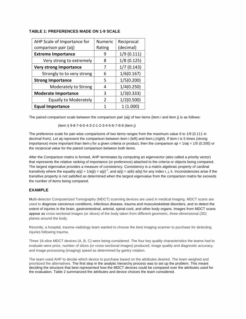
TABLE 1: PREFERENCES MADE ON 1-9 SCALE

AHP Scale of Importance for comparison pair (aij)

Numeric Rating

Reciprocal (decimal)

Extreme Importance 9 1/9 (0.111)

Very strong to extremely 8 1/8 (0.125)

Very strong Importance 7 1/7 (0.143)

Strongly to to very strong 6 1/6(0.167)

Strong Importance 5 1/5(0.200)

Moderately to Strong 4 1/4(0.250)

Moderate Importance 3 1/3(0.333)

Equally to Moderately 2 1/2(0.500)

Equal Importance 1 1 (1.000)

The paired comparison scale between the comparison pair (aij) of two items (item i and item j) is as follows:

(item i) 9-8-7-6-5-4-3-2-1-2-3-4-5-6-7-8-9 (item j) The preference scale for pair-wise comparisons of two items ranges from the maximum value 9 to 1/9 (0.111 in

decimal from). Let aij represent the comparison between item-i (left) and item-j (right). If item-i is 5 times (strong

importance) more important than item-j for a given criteria or product, then the comparison aji = 1/aij = 1/5 (0.200) or

the reciprocal value for the paired comparison between both items.

After the Comparison matrix is formed, AHP terminates by computing an eigenvector (also called a priority vector)

that represents the relative ranking of importance (or preference) attached to the criteria or objects being compared.

The largest eigenvalue provides a measure of consistency. Consistency is a matrix algebraic property of cardinal

transitivity where the equality a(ij) = 1/a(ji) = a(ji)-1

, and a(ij) = a(ik) a(kj) for any index i, j, k. Inconsistencies arise if the

transitive property is not satisfied as determined when the largest eigenvalue from the comparison matrix far exceeds

the number of items being compared.

EXAMPLE

Multi-detector Computerized Tomography (MDCT) scanning devices are used in medical imaging. MDCT scans are

used to diagnose cancerous conditions, infectious disease, trauma and musculoskeletal disorders, and to detect the

extent of injuries in the brain, gastrointestinal, arterial, spinal cord, and other body organs. Images from MDCT scans

appear as cross-sectional images (or slices) of the body taken from different geometric, three-dimensional (3D)

planes around the body.

Recently, a hospital, trauma–radiology team wanted to choose the best imaging scanner to purchase for detecting

injuries following trauma.

Three 16-slice MDCT devices (A, B, C) were being considered. The four key quality characteristics the teams had to

evaluate were price, number of slices (or cross-sectional images) produced, image quality and diagnostic accuracy,

and image-processing (imaging) speed as determined by gantry rotation.

The team used AHP to decide which device to purchase based on the attributes desired. The team weighed and prioritized the alternatives. The first step in the analytic hierarchy process was to set up the problem. This meant deciding the structure that best represented how the MDCT devices could be compared over the attributes used for the evaluation. Table 2 summarized the attributes and device choices the team considered.

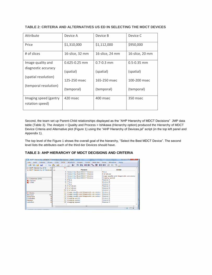
TABLE 2: CRITERIA AND ALTERNATIVES US ED IN SELECTING THE MDCT DEVICES

Attribute Device A Device B Device C

Price $1,310,000 $1,112,000 $950,000

# of slices 16-slice, 32 mm 16-slice, 24 mm 16-slice, 20 mm

Image quality and

diagnostic accuracy

(spatial resolution)

(temporal resolution)

0.625-0.25 mm

(spatial)

125-250 msec

(temporal)

0.7-0.3 mm

(spatial)

165-250 msec

(temporal)

0.5-0.35 mm

(spatial)

100-200 msec

(temporal)

Imaging speed (gantry

rotation speed)

420 msec 400 msec 350 msec

Second, the team set up Parent-Child relationships displayed as the “AHP Hierarchy of MDCT Decisions” JMP data

table (Table 3). The Analyze > Quality and Process > Ishikawa (Hierarchy option) produced the Hierarchy of MDCT

Device Criteria and Alternative plot (Figure 1) using the “AHP Hierarchy of Devices.jsl” script (in the top left panel and

Appendix 1).

The top level of the Figure 1 shows the overall goal of the hierarchy, “Select the Best MDCT Device”. The second

level lists the attributes each of the third-tier Devices should have.

TABLE 3: AHP HIERARCHY OF MDCT DECISIONS AND CRITERIA

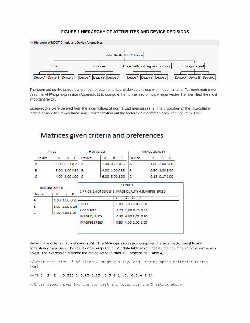
FIGURE 1 HIERARCHY OF ATTRIBUTES AND DEVICE DECISIONS

The team set up the paired comparison of each criteria and device choices within each criteria. For each matrix we

used the AHPexpr expression (Appendix 2) to compute the normalized principal eigenvector that identified the most

important factor.

Eigenvectors were derived from the eigenvalues of normalized measures (i.e., the proportion of the row/column

factors divided the row/column sum). Normalization put the factors on a common scale ranging from 0 to 1.

Below is the criteria matrix shown in JSL. The AHPexpr expression computed the eigenvector weights and

consistency measures. The results were output to a JMP data table which labeled the columns from the rownames

object. The expression returned the dta object for further JSL processing (Table 4).

//Enter the Price, # of slices, Image quality, and Imaging speed criterion matrix

(4x4)

X=[1 3 2 2 , 0.333 1 0.25 0.25, 0.5 4 1 .5, 0.5 4 2 1];

//Enter label names for the row list and total for the X matrix above.

//The last item "Sum" (in the rownames list) is the row sum of the

// row entries. Similarly, the script produces column sum totals.

rownames={"Price", "# of slices", "Image quality", "Imaging speed", "Sum", "Priority

Weight", "Geometric Mean eigenvector"};

//name for the normalized matrix of X above

nmtxname =expr("Relative Decimal Value Matrix for the Device selection criteria

(Price, # of slices,image quality, image processing speed).jmp");

AHPexpr;

dta<< New Column( "Criteria", Character,Nominal,

Set Values({"Price", "# of slices", "Image quality", "Imaging Speed",

"Sum"} ) );

Device_selection_weight = weight ;

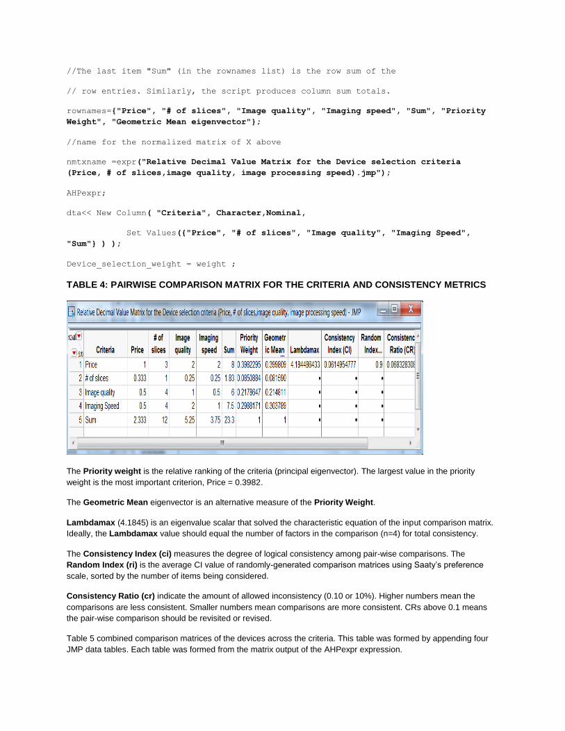
TABLE 4: PAIRWISE COMPARISON MATRIX FOR THE CRITERIA AND CONSISTENCY METRICS

The Priority weight is the relative ranking of the criteria (principal eigenvector). The largest value in the priority

weight is the most important criterion, Price = 0.3982.

The Geometric Mean eigenvector is an alternative measure of the Priority Weight.

Lambdamax (4.1845) is an eigenvalue scalar that solved the characteristic equation of the input comparison matrix.

Ideally, the Lambdamax value should equal the number of factors in the comparison (n=4) for total consistency.

The Consistency Index (ci) measures the degree of logical consistency among pair-wise comparisons. The

Random Index (ri) is the average CI value of randomly-generated comparison matrices using Saaty’s preference

scale, sorted by the number of items being considered.

Consistency Ratio (cr) indicate the amount of allowed inconsistency (0.10 or 10%). Higher numbers mean the

comparisons are less consistent. Smaller numbers mean comparisons are more consistent. CRs above 0.1 means

the pair-wise comparison should be revisited or revised.

Table 5 combined comparison matrices of the devices across the criteria. This table was formed by appending four

JMP data tables. Each table was formed from the matrix output of the AHPexpr expression.

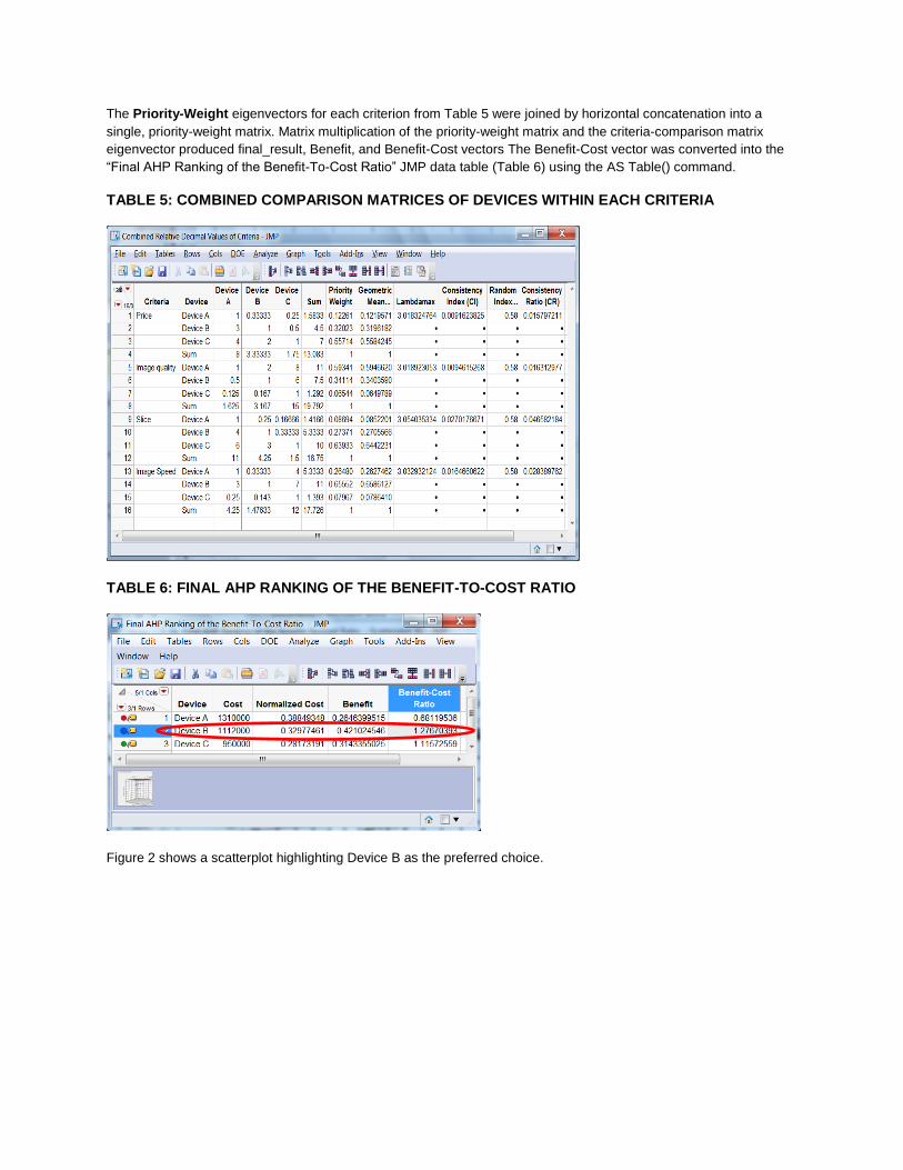
The Priority-Weight eigenvectors for each criterion from Table 5 were joined by horizontal concatenation into a

single, priority-weight matrix. Matrix multiplication of the priority-weight matrix and the criteria-comparison matrix

eigenvector produced final_result, Benefit, and Benefit-Cost vectors The Benefit-Cost vector was converted into the

“Final AHP Ranking of the Benefit-To-Cost Ratio” JMP data table (Table 6) using the AS Table() command.

TABLE 5: COMBINED COMPARISON MATRICES OF DEVICES WITHIN EACH CRITERIA

TABLE 6: FINAL AHP RANKING OF THE BENEFIT-TO-COST RATIO

Figure 2 shows a scatterplot highlighting Device B as the preferred choice.

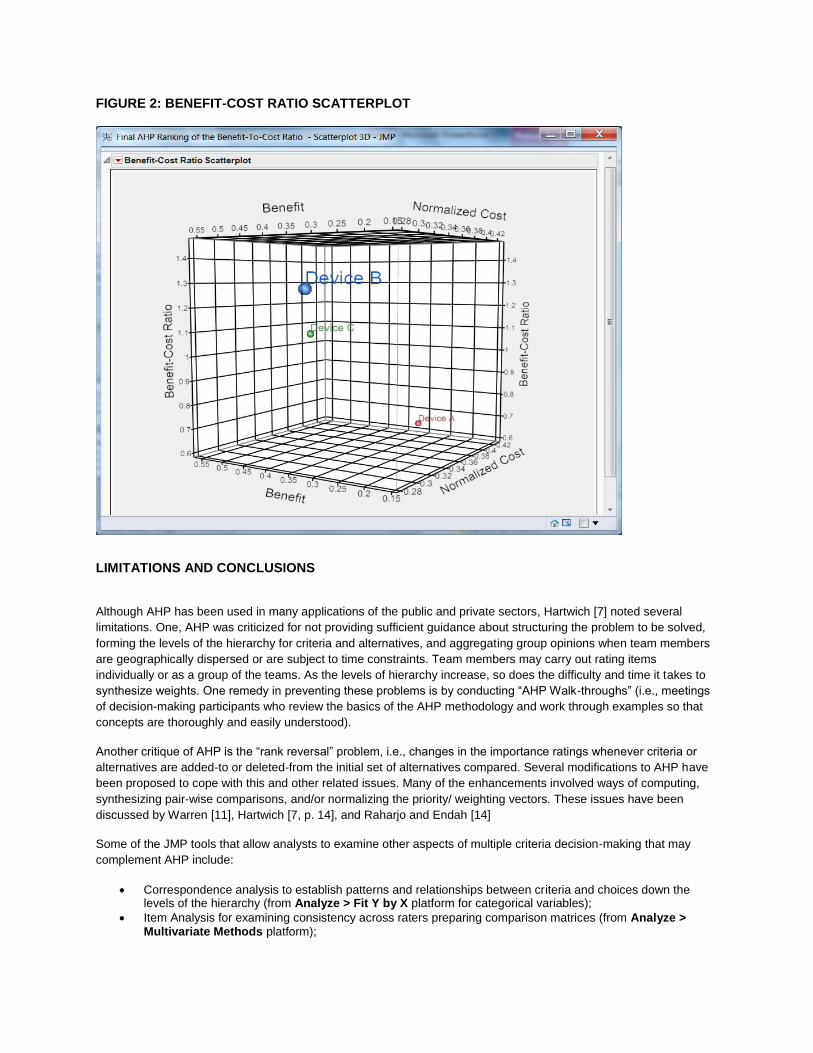
FIGURE 2: BENEFIT-COST RATIO SCATTERPLOT

LIMITATIONS AND CONCLUSIONS

Although AHP has been used in many applications of the public and private sectors, Hartwich [7] noted several

limitations. One, AHP was criticized for not providing sufficient guidance about structuring the problem to be solved,

forming the levels of the hierarchy for criteria and alternatives, and aggregating group opinions when team members

are geographically dispersed or are subject to time constraints. Team members may carry out rating items

individually or as a group of the teams. As the levels of hierarchy increase, so does the difficulty and time it takes to

synthesize weights. One remedy in preventing these problems is by conducting “AHP Walk-throughs” (i.e., meetings

of decision-making participants who review the basics of the AHP methodology and work through examples so that

concepts are thoroughly and easily understood).

Another critique of AHP is the “rank reversal” problem, i.e., changes in the importance ratings whenever criteria or

alternatives are added-to or deleted-from the initial set of alternatives compared. Several modifications to AHP have

been proposed to cope with this and other related issues. Many of the enhancements involved ways of computing,

synthesizing pair-wise comparisons, and/or normalizing the priority/ weighting vectors. These issues have been

discussed by Warren [11], Hartwich [7, p. 14], and Raharjo and Endah [14]

Some of the JMP tools that allow analysts to examine other aspects of multiple criteria decision-making that may

complement AHP include:

Correspondence analysis to establish patterns and relationships between criteria and choices down the levels of the hierarchy (from Analyze > Fit Y by X platform for categorical variables);

Item Analysis for examining consistency across raters preparing comparison matrices (from Analyze > Multivariate Methods platform);

Principal components to extract dimensions defined by the criteria and options (from Graph > Scatterplot 3D platform).

Conjoint Analysis which may be implemented by using JMP’s DOE > Custom Design platform to create a

design matrix data table that generates scenarios of product attributes, levels, and possible options. The Data table may be saved until data to fill the preference ratings for the Y column(s) are available. The data may be analyzed using the model fitting tools from the Analyze platform. Conjoint designs and analysis

were created in JMP Version 8. Pre-version 8 did not have this.

Despite AHP’s criticisms, the methodology has been popular, fairly simple to apply, and is the leading approach used

for multi-criteria decision-making, see Hochbaum and Levin [15]. Other decision-making alternatives have limitations

similar to AHP.

NASA used AHP to design mission-success factors for human MARS Exploration, see Flaherty et al. [6].

Ho and Emrouznejad [8] used SAS/OR, AHP, and Goal Programming to evaluate warehouse performance delivering

products to customers in a logistic distribution network. Emrouznejad and Ho [5] provided other AHP examples.

AHP was used to extract judgmental forecast adjustments of Myrtle Beach, SC golf-course demand [19].

The AHPexpr in JSL performs the basic AHP calculations found in most AHP web-based calculators (e.g.,

www.123AHP.com) or Excel spreadsheets. The AHPexpr expression is customizable, flexible, and expandable. Data

can be input as one multi-dimensional matrix. Most AHP spreadsheets require users to pick specific sheets of

different sizes for paired-comparison data entry. The matrices from the AHPexpr expression can be output as JMP

data tables via the As Table () command in JMP JSL for further data shaping, visualization, and analysis.

This presentation has shown how JMP’s scripting tools can be used to implement the AHP methodology. The data

tables produced are typical of the results found in standard AHP reports. I wrote a similar AHP subroutine that runs

on SAS/IML.

REFERENCES

1. T.L. Saaty, 1977, “A Scaling Method for Priorities in Hierarchical Structures”, Journal of Mathematical Psychology,

15, 234-281.

2. T.L. Saaty, 1980, The Analytic Hierarchy Process, McGraw-Hill, New York.

3. T.L. Saaty 1999, Decision Making for Leaders, 3rd

ed., RWS Publications: Pittsburgh, PA.

4. K. Teknomo, 2006, Analytic Hierarchy Process (AHP) Tutorial, Available from

http://people.revoledu.com/kardi/tutorial/AHP/.

5. A. Emrouznejad and W. Ho, 2011, Applied Operational Research with SAS (2011, Chapter 8). Chapman and

Hall/CRC. Boca Raton, FL.

6. K. Flaherty, M. Grant, et. al., “ESAS-Derived Earth Departure Stage Design for Human Mars Exploration” Available

from http://education.ksc.nasa.gov/esmdspacegrant/Documents/GT_South_SE_Paper.pdf, accessed 03/12/12.

7. F. Hartwich, 1999, “Weighing of Agricultural Research Results: Strength and Limitations of the Analytical Hierarchy

Process (AHP)”, Available from http://www.uni-hohenheim.de/i490a/dps/1999/09-99/dp99-09.pdf, accessed 03/23/07.

8. S.T. Foster and G. LaCava’s data from the AHP.ppt presentation, “The Analytical Hierarchy Process: A Step-by-

Step Approach,” Available from https://acc.dau.mil/CommunityBrowser.aspx, accessed 03/23/07.

9. W. Ho and A. Emrouznejad, 2009, “Multi-criteria logistics distribution network design using SAS/OR,” Expert Systems With Applications, 36, 7288–7298.

10. J. R. Grandzol, “Improving the Faculty Selection Process in Higher Education: a Case for the Analytic Hierarchy

Process,” IR Applications Using Advanced Tools, Techniques, and Methodologies, vol. 6, August 24, 2005,

Association for Institutional Research, Available from http://airweb.org/page.asp?page=295 , accessed 04/12/07.

11. J. Afarin, “Method for Optimizing Research Allocation in a Government Organization,“ NASA Technical

Memorandum 106690, 1994, Available from

http://ntrs.nasa.gov/archive/nasa/casi.ntrs.nasa.gov/19950004838_1995104838.pdf accessed 04/12/07.

12. J. Warren, “Uncertainties in the Analytic Hierarchy Process,” 2004, Available from

http://www.dsto.defence.gov.au/publications/3476/DSTO-TN-0597.pdf, accessed 4/15/07.

13. L. E. Shirland and R.R. Jesse, “Prioritizing Customer Requirements Using Goal Programming,” 1997, American

Society for Quality’s 51st Annual Quality Congress Proceedings, 51. Orlando, FL, 297-308.

14. H. Raharjo and D. Endah, 2006, “Evaluating Relationship of consistency Ratio and Number of Alternatives on

Rank Reversal in the AHP,” Quality Engineering, 18: 39-46.

15. D.S Hochbaum and A. Levin, 2006, “Methodologies and algorithms for group ranking decisions,” p.8, Available

from http://pluto.mscc.huji.ac.il/~levinas/nsf.pdf , accessed 4/15/07.

16. R.L Keeney and H. Raiffa, 1976, Decisions with Multiple Objectives: Preference and Value Tradeoffs, Wiley: New

York.

17. P. Szwed et al, “A Bayesian Paired Comparison Approach for Relative Accident Probability Assessment with

Covariate Information,” Available from

http://www.seas.gwu.edu/~dorpjr/Publications/JournalPapers/EJOR%202004.pdf accessed 04/12/07.

18. D.L. Hallowell , “View via Tollgates in Six Sigma for Software Orientation,” Available from

http://software.isixsigma.com/library/content/c040107b.asp, accessed 4/19/07.

19. S. Parrot, 2012, “Guest Blogger: Len Tashman previews Winter 2012 issue of Foresight,” Available from

http://blogs.sas.com/content/forecasting/2012/01/18/guest-blogger-len-tashman-previews-winter-2012-issue-of-

foresight/.

ACKNOWLEDGMENTS I thank Kathirkamanathan Shanmuganathan for his contributions to this paper. I thank Lucia Ward-Alexander for her review and editorial assistance.

CONTACT INFORMATION

Your comments and questions are valued and encouraged. Contact the author at:

Melvin Alexander

Phone (410) 458-7129

E-mail: Melvin.alexander@verizon.net

JMP, SAS and all other SAS Institute, Inc. product or service names are registered trademarks or trademarks of SAS

Institute Inc. in the USA and other countries. ® indicates USA registration.

Other brand and product names are registered trademarks or trademarks of their respective companies.

APPENDIX 1: JSL SCRIPT TO CREATE THE AHP HIERARCHY OF MDCT SELECTION DECISIONS

New Table( "AHP Hierarchy of MDCT Selection Decisions",

Add Rows( 16 ),

New Script("AHP Hierarchy of Devices",

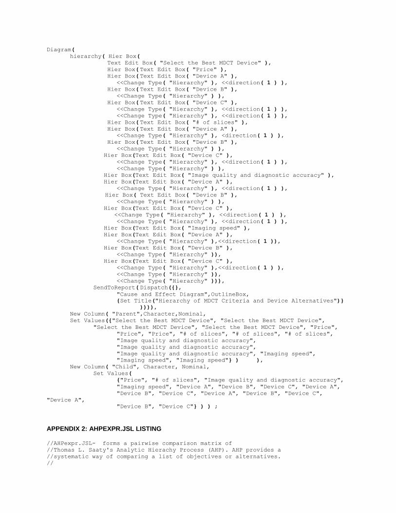
Diagram(

hierarchy( Hier Box(

Text Edit Box( "Select the Best MDCT Device" ),

Hier Box( Text Edit Box( "Price" ),

Hier Box( Text Edit Box( "Device A" ),

<<Change Type( "Hierarchy" ), <<direction( 1 ) ),

Hier Box( Text Edit Box( "Device B" ),

<<Change Type( "Hierarchy" ) ),

Hier Box( Text Edit Box( "Device C" ),

<<Change Type( "Hierarchy" ), <<direction( 1 ) ),

<<Change Type( "Hierarchy" ), <<direction( 1 ) ),

Hier Box( Text Edit Box( "# of slices" ),

Hier Box( Text Edit Box( "Device A" ),

<<Change Type( "Hierarchy" ), <direction( 1 ) ),

Hier Box( Text Edit Box( "Device B" ),

<<Change Type( "Hierarchy" ) ),

Hier Box(Text Edit Box( "Device C" ),

<<Change Type( "Hierarchy" ), <<direction( 1 ) ),

<<Change Type( "Hierarchy" ) ),

Hier Box(Text Edit Box( "Image quality and diagnostic accuracy" ),

Hier Box(Text Edit Box( "Device A" ),

<<Change Type( "Hierarchy" ), <<direction( 1 ) ),

Hier Box( Text Edit Box( "Device B" ),

<<Change Type( "Hierarchy" ) ),

Hier Box(Text Edit Box( "Device C" ),

<<Change Type( "Hierarchy" ), <<direction( 1 ) ),

<<Change Type( "Hierarchy" ), <<direction( 1 ) ),

Hier Box(Text Edit Box( "Imaging speed" ),

Hier Box(Text Edit Box( "Device A" ),

<<Change Type( "Hierarchy" ),<<direction( 1 )),

Hier Box(Text Edit Box( "Device B" ),

<<Change Type( "Hierarchy" )),

Hier Box(Text Edit Box( "Device C" ),

<<Change Type( "Hierarchy" ),<<direction( 1 ) ),

<<Change Type( "Hierarchy" )),

<<Change Type( "Hierarchy" ))),

SendToReport( Dispatch({},

"Cause and Effect Diagram",OutlineBox,

{Set Title("Hierarchy of MDCT Criteria and Device Alternatives")}

)))),

New Column( "Parent",Character,Nominal,

Set Values({"Select the Best MDCT Device", "Select the Best MDCT Device",

"Select the Best MDCT Device", "Select the Best MDCT Device", "Price",

"Price", "Price", "# of slices", "# of slices", "# of slices",

"Image quality and diagnostic accuracy",

"Image quality and diagnostic accuracy",

"Image quality and diagnostic accuracy", "Imaging speed",

"Imaging speed", "Imaging speed"} ) ),

New Column( "Child", Character, Nominal,

Set Values(

{"Price", "# of slices", "Image quality and diagnostic accuracy",

"Imaging speed", "Device A", "Device B", "Device C", "Device A",

"Device B", "Device C", "Device A", "Device B", "Device C",

"Device A",

"Device B", "Device C"} ) ) ;

APPENDIX 2: AHPEXPR.JSL LISTING

//AHPexpr.JSL- forms a pairwise comparison matrix of

//Thomas L. Saaty's Analytic Hierachy Process (AHP). AHP provides a

//systematic way of comparing a list of objectives or alternatives.

//

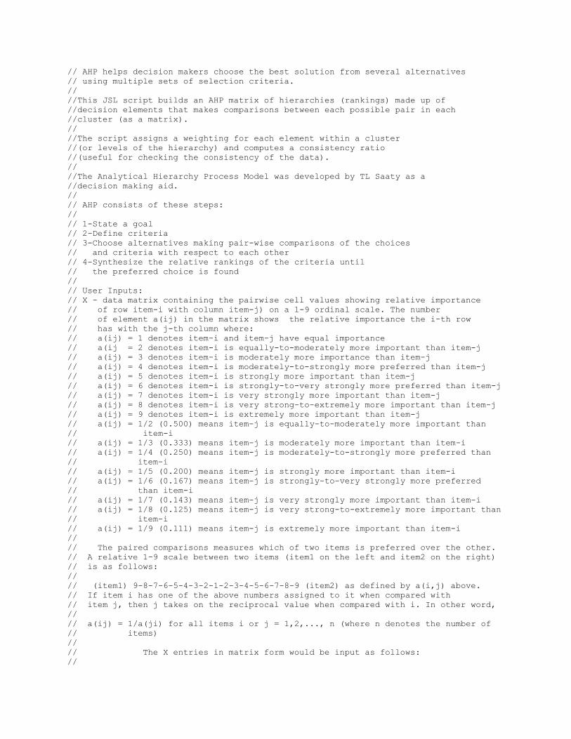
// AHP helps decision makers choose the best solution from several alternatives

// using multiple sets of selection criteria.

//

//This JSL script builds an AHP matrix of hierarchies (rankings) made up of

//decision elements that makes comparisons between each possible pair in each

//cluster (as a matrix).

//

//The script assigns a weighting for each element within a cluster

//(or levels of the hierarchy) and computes a consistency ratio

//(useful for checking the consistency of the data).

//

//The Analytical Hierarchy Process Model was developed by TL Saaty as a

//decision making aid.

//

// AHP consists of these steps:

//

// 1-State a goal

// 2-Define criteria

// 3-Choose alternatives making pair-wise comparisons of the choices

// and criteria with respect to each other

// 4-Synthesize the relative rankings of the criteria until

// the preferred choice is found

//

// User Inputs:

// X - data matrix containing the pairwise cell values showing relative importance

// of row item-i with column item-j) on a 1-9 ordinal scale. The number

// of element a(ij) in the matrix shows the relative importance the i-th row

// has with the j-th column where:

// a(ij) = 1 denotes item-i and item-j have equal importance

// a(ij = 2 denotes item-i is equally-to-moderately more important than item-j

// a(ij) = 3 denotes item-i is moderately more importance than item-j

// a(ij) = 4 denotes item-i is moderately-to-strongly more preferred than item-j

// a(ij) = 5 denotes item-i is strongly more important than item-j

// a(ij) = 6 denotes item-i is strongly-to-very strongly more preferred than item-j

// a(ij) = 7 denotes item-i is very strongly more important than item-j

// a(ij) = 8 denotes item-i is very strong-to-extremely more important than item-j

// a(ij) = 9 denotes item-i is extremely more important than item-j

// a(ij) = 1/2 (0.500) means item-j is equally-to-moderately more important than

// item-i

// a(ij) = 1/3 (0.333) means item-j is moderately more important than item-i

// a(ij) = 1/4 (0.250) means item-j is moderately-to-strongly more preferred than

// item-i

// a(ij) = 1/5 (0.200) means item-j is strongly more important than item-i

// a(ij) = 1/6 (0.167) means item-j is strongly-to-very strongly more preferred

// than item-i

// a(ij) = 1/7 (0.143) means item-j is very strongly more important than item-i

// a(ij) = 1/8 (0.125) means item-j is very strong-to-extremely more important than

// item-i

// a(ij) = 1/9 (0.111) means item-j is extremely more important than item-i

//

// The paired comparisons measures which of two items is preferred over the other.

// A relative 1-9 scale between two items (item1 on the left and item2 on the right)

// is as follows:

//

// (item1) 9-8-7-6-5-4-3-2-1-2-3-4-5-6-7-8-9 (item2) as defined by a(i,j) above.

// If item i has one of the above numbers assigned to it when compared with

// item j, then j takes on the reciprocal value when compared with i. In other word,

//

// a(ij) = 1/a(ji) for all items i or j = 1,2,..., n (where n denotes the number of

// items)

//

// The X entries in matrix form would be input as follows:

//

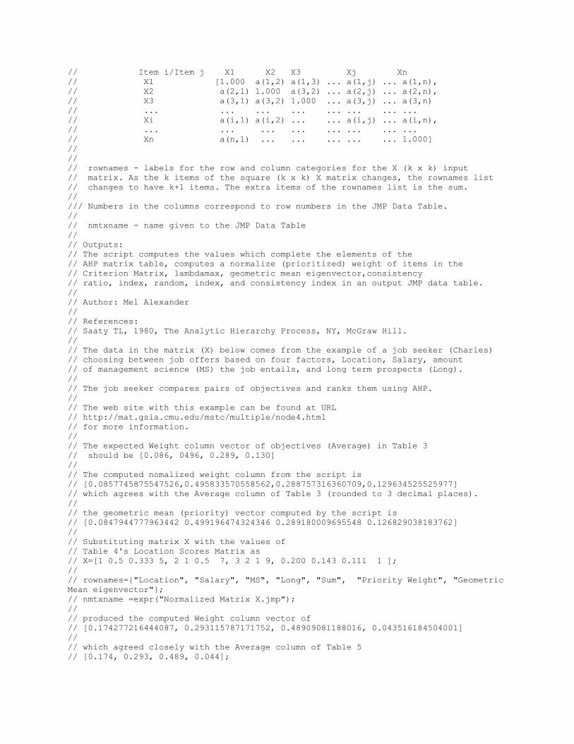
// Item i/Item j X1 X2 X3 Xj Xn

// X1 [1.000 a(1,2) a(1,3) ... a(1,j) ... a(1,n),

// X2 a(2,1) 1.000 a(3,2) ... a(2,j) ... a(2,n),

// X3 a(3,1) a(3,2) 1.000 ... a(3,j) ... a(3,n)

// ... ... ... ... ... ... ... ...

// Xi a(i,1) a(i,2) ... ... a(i,j) ... a(i,n),

// ... ... ... ... ... ... ... ...

// Xn a(n,1) ... ... ... ... ... 1.000]

//

//

// rownames - labels for the row and column categories for the X (k x k) input

// matrix. As the k items of the square (k x k) X matrix changes, the rownames list

// changes to have k+1 items. The extra items of the rownames list is the sum.

//

/// Numbers in the columns correspond to row numbers in the JMP Data Table.

//

// nmtxname - name given to the JMP Data Table

//

// Outputs:

// The script computes the values which complete the elements of the

// AHP matrix table, computes a normalize (prioritized) weight of items in the

// Criterion Matrix, lambdamax, geometric mean eigenvector,consistency

// ratio, index, random, index, and consistency index in an output JMP data table.

//

// Author: Mel Alexander

//

// References:

// Saaty TL, 1980, The Analytic Hierarchy Process, NY, McGraw Hill.

//

// The data in the matrix (X) below comes from the example of a job seeker (Charles)

// choosing between job offers based on four factors, Location, Salary, amount

// of management science (MS) the job entails, and long term prospects (Long).

//

// The job seeker compares pairs of objectives and ranks them using AHP.

//

// The web site with this example can be found at URL

// http://mat.gsia.cmu.edu/mstc/multiple/node4.html

// for more information.

//

// The expected Weight column vector of objectives (Average) in Table 3

// should be [0.086, 0496, 0.289, 0.130]

//

// The computed nomalized weight column from the script is

// [0.0857745875547526,0.495833570558562,0.288757316360709,0.129634525525977]

// which agrees with the Average column of Table 3 (rounded to 3 decimal places).

//

// the geometric mean (priority) vector computed by the script is

// [0.0847944777963442 0.499196474324346 0.289180009695548 0.126829038183762]

//

// Substituting matrix X with the values of

// Table 4's Location Scores Matrix as

// X=[1 0.5 0.333 5, 2 1 0.5 7, 3 2 1 9, 0.200 0.143 0.111 1 ];

//

// rownames={"Location", "Salary", "MS", "Long", "Sum", "Priority Weight", "Geometric

Mean eigenvector"};

// nmtxname =expr("Normalized Matrix X.jmp");

//

// produced the computed Weight column vector of

// [0.174277216444087, 0.293115787171752, 0.48909081188016, 0.043516184504001]

//

// which agreed closely with the Average column of Table 5

// [0.174, 0.293, 0.489, 0.044];

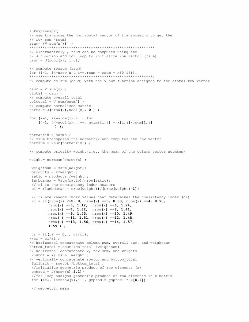
AHPexpr=expr(

// use transpose the horizontal vector of transposed x to get the

// row sum (rsum)

rsum= (V sum(x`))` ;

/********************************************************

// Alternatively , rsum can be computed using the

// J function and for loop to initialize row vector (rsum)

rsum = J(ncol(x), 1,0);

// compute rowsum (rsum)

for (i=1, i<=nrow(x), i++,rsum = rsum + x[0,i];);

********************************************************/

// compute colsum (csum) with the V sum function assigned to the ctotal row vector

csum = V sum(x) ;

ctotal = csum ;

// compute overall total

coltotal = V sum(csum`) ;

// compute normalized matrix

norms = J(nrow(x),ncol(x), 0 ) ;

for (i=1, i<=nrow(x),i++, for

(j=1, j<=ncol(x), j++, norms[i,j] = x[i,j]/csum[1,j]

) );

normatrix = norms ;

// Vsum transposes the normatrix and computes the row vector

normsum = Vsum(normatrix`) ;

// compute priority weight(i.e., the mean of the column vector normsum)

weight= normsum`/nrow(x) ;

weightsum = Vsum(weight);

products = x*weight ;

ratio = products:/weight ;

lambdamax = Vsum(ratio)/nrow(ratio);

// ci is the consistancy index measure

ci = (lambdamax - nrow(weight))/(nrow(weight)-1);

// ri are random index values that determines the consistency index (ci)

ri = if(nrow(x) <=2, 0, nrow(x) ==3, 0.58, nrow(x) ==4, 0.90,

nrow(x) ==5, 1.12, nrow(x) ==6, 1.24,

nrow(x) ==7, 1.32, nrow(x) ==8, 1.41,

nrow(x) ==9, 1.45, nrow(x) ==10, 1.49,

nrow(x) ==11, 1.51, nrow(x) ==12, 1.48,

nrow(x) ==13, 1.56, nrow(x) ==14, 1.57,

1.59 ) ;

cr = if(ri == 0,., ci/ri);

//cr = ci/ri ;

// horizontal concatenate column sum, overall sum, and weightsum

bottom_total = csum||coltotal||weightsum;

// horizontal concatenate x, row sum, and weights

rowtot = x||rsum||weight ;

// vertically concatenate rowtot and bottom_total

fullcrit = rowtot|/bottom_total ;

//initialize geometric product of row elements (x)

gmprod = J(nrow(x),1,1);

//for loop assigns geometric product of row elements in x matrix

for (i=1, i<=nrow(x),i++, gmprod = gmprod :* x[0,i]);

// geometric mean

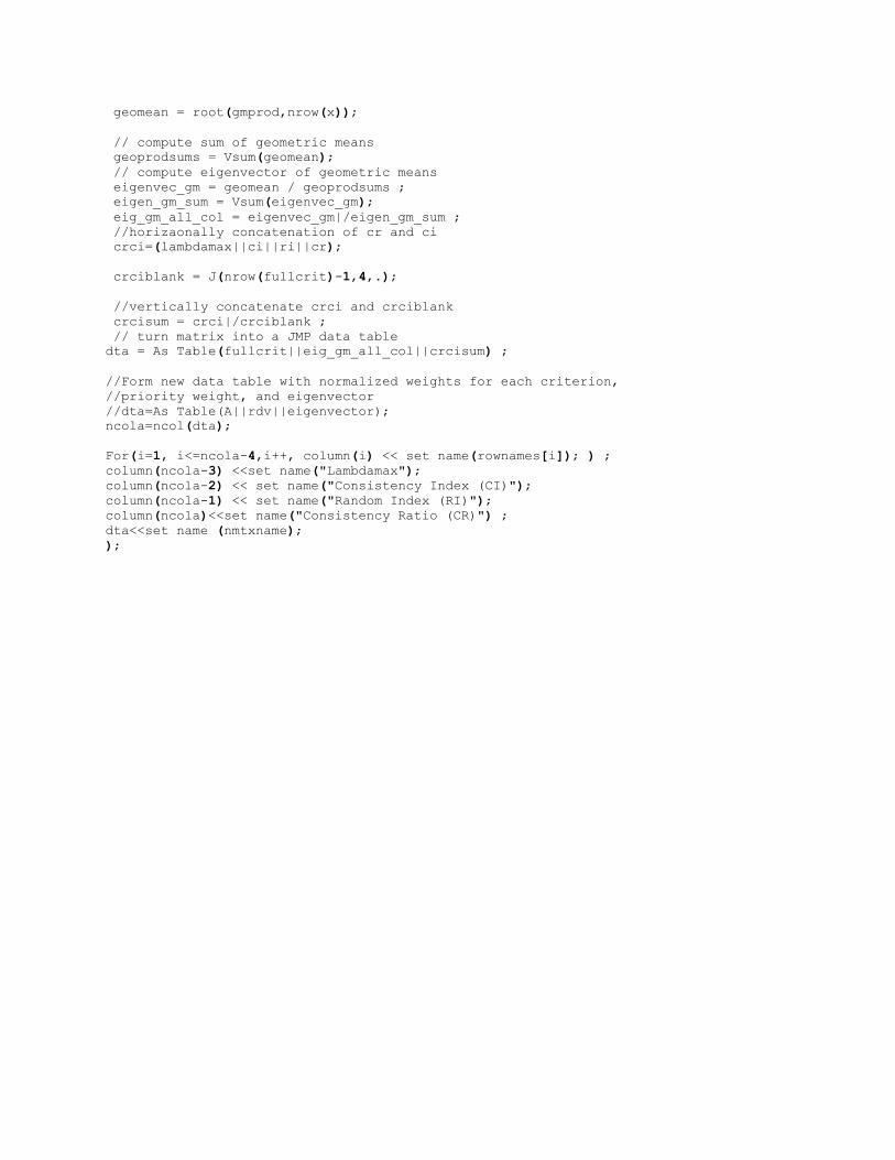
geomean = root(gmprod,nrow(x));

// compute sum of geometric means

geoprodsums = Vsum(geomean);

// compute eigenvector of geometric means

eigenvec_gm = geomean / geoprodsums ;

eigen_gm_sum = Vsum(eigenvec_gm);

eig_gm_all_col = eigenvec_gm|/eigen_gm_sum ;

//horizaonally concatenation of cr and ci

crci=(lambdamax||ci||ri||cr);

crciblank = J(nrow(fullcrit)-1,4,.);

//vertically concatenate crci and crciblank

crcisum = crci|/crciblank ;

// turn matrix into a JMP data table

dta = As Table(fullcrit||eig_gm_all_col||crcisum) ;

//Form new data table with normalized weights for each criterion,

//priority weight, and eigenvector

//dta=As Table(A||rdv||eigenvector);

ncola=ncol(dta);

For(i=1, i<=ncola-4,i++, column(i) << set name(rownames[i]); ) ;

column(ncola-3) <<set name("Lambdamax");

column(ncola-2) << set name("Consistency Index (CI)");

column(ncola-1) << set name("Random Index (RI)");

column(ncola)<<set name("Consistency Ratio (CR)") ;

dta<<set name (nmtxname);

);