Deciphering the Seismic Signature of the Edvard Grieg Field, North Sea Abel O. Ndingwan*, Odd Kolbjørnsen, Knut R. Straith and Morten D. Bjerke (Lundin Norway AS)

Summary

We present a case of seismic reservoir characterization within a multi-source depositional setting. To resolve issues of non-

uniqueness between intrinsic reservoir properties and the seismic data, we use a probabilistic approach. Stochastic rock physics

relationships are used to establish a link between elastic parameters and various lithology classes. We highlight the importance of

concurrently using multiple lithological prior models to achieve an improved understanding of the seismic response of the Edvard

Grieg field. Application of a one-step inversion approach, which assesses the direct conditional (posterior) distribution of elastic

parameters, yields improved reservoir prediction particularly in regions where the reservoir sandstones are thin. Quantitative

prediction and interpretation of impedances and lithology volumes is done in light of selected models and associated uncertainties.

Introduction

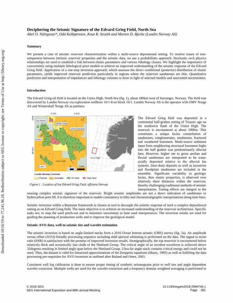
The Edvard Grieg oil field is located on the Utsira High, North Sea (fig. 1), about 180km west of Stavanger, Norway. The field was

discovered by Lundin Norway via exploration wellbore 16/1-8 on block 16/1. Lundin Norway AS is the operator with OMV Norge

AS and Wintershall Norge AS as partners.

The Edvard Grieg field was deposited in a

continental half-graben setting of Triassic age on

the southwest flank of the Utsira High. The

reservoir is encountered at about 1900m. This

constitutes a unique facies constellation of

sandstones, conglomerates, mudstones, fractured

and weathered basement. Multi-source sediment

input from neighboring structural basement highs

into the half graben was predominantly alluvial

fans. However, higher net to gross aeolian and

fluvial sandstones are interpreted to be trans-

axially deposited relative to the alluvial fan

systems. Inter-dune deposits as well as lacustrine

and floodplain mudstones are included in the

ensemble. Significant variability in geologic

facies, thus elastic properties, is observed over

relatively short distances within the reservoir,

thereby challenging traditional methods of seismic

interpretation. Tuning effects are integral to the

ensuing complex seismic signature of the reservoir. Bright seismic amplitudes are not a direct indication of sandstones or

hydrocarbon pore fill. It is therefore important to enable consistency in litho and chronostratigraphic interpretations along time lines.

Seismic inversion within a Bayesian framework is chosen as tool to decouple the seismic response of such a complex depositional

setting as on Edvard Grieg field. The main objective is to achieve an increased understanding of the reservoir architecture. Specific

tasks are; to map the sand pinch-out and to minimize uncertainty in base sand interpretation. The inversion results are used for

guiding the planning of production wells and to improve the geological model.

Seismic AVO data, well-to-seismic ties and wavelet estimation

The seismic inversion is based on angle-limited stacks from a 2016 Ocean bottom seismic (OBS) survey (fig. 2a). An amplitude

versus offset (AVO) friendly processing sequence including mild spectral whitening is performed on the data. The signal to noise

ratio (SNR) is satisfactory with the promise of improved inversion results. Stratigraphically, the top reservoir is encountered below

relatively thick and acoustically fast chalk of the Shetland Group. The critical angle of an incident waveform is achieved above

32degrees resulting in limited angle span below the Shetland Group. Ultra-far angle stack contains critical energy and could not be

used. Thus, the dataset is valid for linearized approximations of the Zeoppritz equations (Shuey, 1985) as well as fulfilling the data

processing pre-requisites for AVO inversion as outlined after Buland and Omre, 2003.

Consistent well log calibration is done to ensure proper timing of synthetic seismograms prior to well ties and angle dependent

wavelet extraction. Multiple wells are used for the wavelet extraction and a frequency domain weighted averaging is performed to

10.1190/segam2018-2994746.1Page 361

© 2018 SEGSEG International Exposition and 88th annual Meeting

Dow

nloa

ded

10/1

6/19

to 7

7.24

1.96

.18.

Red

istr

ibut

ion

subj

ect t

o SE

G li

cens

e or

cop

yrig

ht; s

ee T

erm

s of

Use

at h

ttp://

libra

ry.s

eg.o

rg/

obtain angle varying wavelets. The quality of the ties and ultimately the estimated wavelets are assessed by goodness-of-fit

measures. That is; fraction of explained variability and mean squared residuals.

Building the inversion model

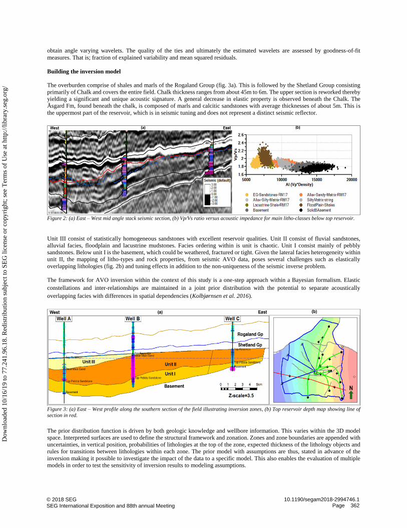
The overburden comprise of shales and marls of the Rogaland Group (fig. 3a). This is followed by the Shetland Group consisting

primarily of Chalk and covers the entire field. Chalk thickness ranges from about 45m to 6m. The upper section is reworked thereby

yielding a significant and unique acoustic signature. A general decrease in elastic property is observed beneath the Chalk. The

Åsgard Fm, found beneath the chalk, is composed of marls and calcitic sandstones with average thicknesses of about 5m. This is

the uppermost part of the reservoir, which is in seismic tuning and does not represent a distinct seismic reflector.

Figure 2: (a) East – West mid angle stack seismic section, (b) Vp/Vs ratio versus acoustic impedance for main litho-classes below top reservoir.

Unit III consist of statistically homogeneous sandstones with excellent reservoir qualities. Unit II consist of fluvial sandstones,

alluvial facies, floodplain and lacustrine mudstones. Facies ordering within is unit is chaotic. Unit I consist mainly of pebbly

sandstones. Below unit I is the basement, which could be weathered, fractured or tight. Given the lateral facies heterogeneity within

unit II, the mapping of litho-types and rock properties, from seismic AVO data, poses several challenges such as elastically

overlapping lithologies (fig. 2b) and tuning effects in addition to the non-uniqueness of the seismic inverse problem.

The framework for AVO inversion within the context of this study is a one-step approach within a Bayesian formalism. Elastic

constellations and inter-relationships are maintained in a joint prior distribution with the potential to separate acoustically

overlapping facies with differences in spatial dependencies (Kolbjørnsen et al. 2016).

Figure 3: (a) East – West profile along the southern section of the field illustrating inversion zones, (b) Top reservoir depth map showing line of

section in red. The prior distribution function is driven by both geologic knowledge and wellbore information. This varies within the 3D model

space. Interpreted surfaces are used to define the structural framework and zonation. Zones and zone boundaries are appended with

uncertainties, in vertical position, probabilities of lithologies at the top of the zone, expected thickness of the lithology objects and

rules for transitions between lithologies within each zone. The prior model with assumptions are thus, stated in advance of the

inversion making it possible to investigate the impact of the data to a specific model. This also enables the evaluation of multiple

models in order to test the sensitivity of inversion results to modeling assumptions.

10.1190/segam2018-2994746.1Page 362

© 2018 SEGSEG International Exposition and 88th annual Meeting

Dow

nloa

ded

10/1

6/19

to 7

7.24

1.96

.18.

Red

istr

ibut

ion

subj

ect t

o SE

G li

cens

e or

cop

yrig

ht; s

ee T

erm

s of

Use

at h

ttp://

libra

ry.s

eg.o

rg/

Three models have been of particular interest. These models are identical with the exception of the parametrization of unit II.

Namely; a full model (FM) which allows for all observed geologic facies in unit II, two specialized models which assumes that unit

II is either dominated by floodplain shale (SM) or an alluvial fan setting dominated by conglomerates (CM).

Results

The inversion algorithm solves for absolute properties and facies probabilities that are directly comparable to impedances and facies

from well data. In addition to the posterior litho-class distributions, we compare the variance in inverted and measured elastic

properties for three models (FM, SM and CM).

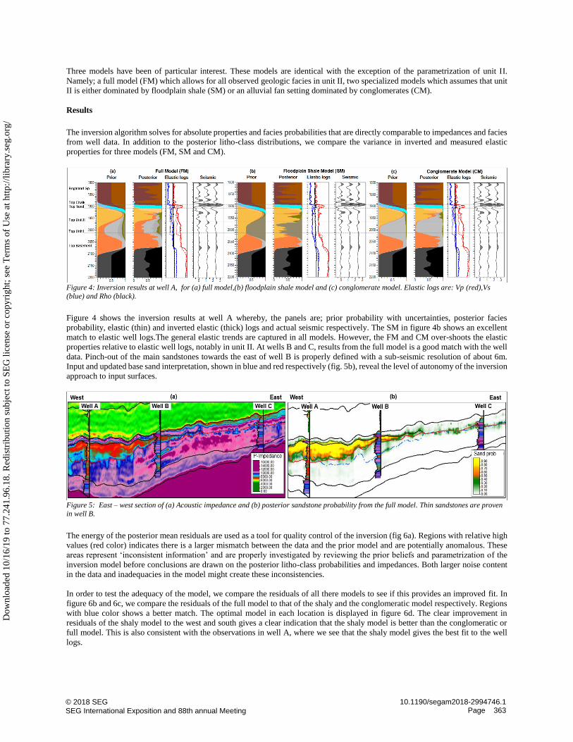
Figure 4: Inversion results at well A, for (a) full model,(b) floodplain shale model and (c) conglomerate model. Elastic logs are: Vp (red),Vs

(blue) and Rho (black). Figure 4 shows the inversion results at well A whereby, the panels are; prior probability with uncertainties, posterior facies

probability, elastic (thin) and inverted elastic (thick) logs and actual seismic respectively. The SM in figure 4b shows an excellent

match to elastic well logs.The general elastic trends are captured in all models. However, the FM and CM over-shoots the elastic

properties relative to elastic well logs, notably in unit II. At wells B and C, results from the full model is a good match with the well

data. Pinch-out of the main sandstones towards the east of well B is properly defined with a sub-seismic resolution of about 6m.

Input and updated base sand interpretation, shown in blue and red respectively (fig. 5b), reveal the level of autonomy of the inversion

approach to input surfaces.

Figure 5: East – west section of (a) Acoustic impedance and (b) posterior sandstone probability from the full model. Thin sandstones are proven

in well B. The energy of the posterior mean residuals are used as a tool for quality control of the inversion (fig 6a). Regions with relative high

values (red color) indicates there is a larger mismatch between the data and the prior model and are potentially anomalous. These

areas represent ‘inconsistent information’ and are properly investigated by reviewing the prior beliefs and parametrization of the

inversion model before conclusions are drawn on the posterior litho-class probabilities and impedances. Both larger noise content

in the data and inadequacies in the model might create these inconsistencies.

In order to test the adequacy of the model, we compare the residuals of all there models to see if this provides an improved fit. In

figure 6b and 6c, we compare the residuals of the full model to that of the shaly and the conglomeratic model respectively. Regions

with blue color shows a better match. The optimal model in each location is displayed in figure 6d. The clear improvement in

residuals of the shaly model to the west and south gives a clear indication that the shaly model is better than the conglomeratic or

full model. This is also consistent with the observations in well A, where we see that the shaly model gives the best fit to the well

logs.

10.1190/segam2018-2994746.1Page 363

© 2018 SEGSEG International Exposition and 88th annual Meeting

Dow

nloa

ded

10/1

6/19

to 7

7.24

1.96

.18.

Red

istr

ibut

ion

subj

ect t

o SE

G li

cens

e or

cop

yrig

ht; s

ee T

erm

s of

Use

at h

ttp://

libra

ry.s

eg.o

rg/

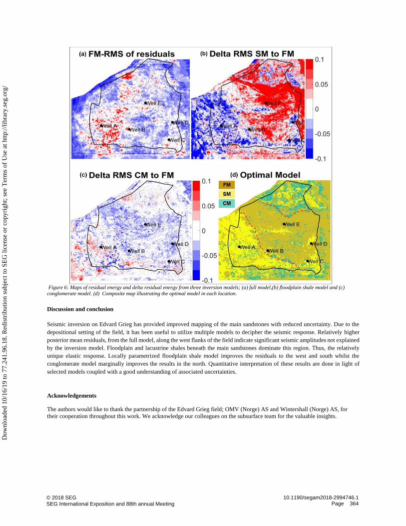
Figure 6: Maps of residual energy and delta residual energy from three inversion models; (a) full model,(b) floodplain shale model and (c)

conglomerate model. (d) Composite map illustrating the optimal model in each location. Discussion and conclusion

Seismic inversion on Edvard Grieg has provided improved mapping of the main sandstones with reduced uncertainty. Due to the

depositional setting of the field, it has been useful to utilize multiple models to decipher the seismic response. Relatively higher

posterior mean residuals, from the full model, along the west flanks of the field indicate significant seismic amplitudes not explained

by the inversion model. Floodplain and lacustrine shales beneath the main sandstones dominate this region. Thus, the relatively

unique elastic response. Locally parametrized floodplain shale model improves the residuals to the west and south whilst the

conglomerate model marginally improves the results in the north. Quantitative interpretation of these results are done in light of

selected models coupled with a good understanding of associated uncertainties.

Acknowledgements

The authors would like to thank the partnership of the Edvard Grieg field; OMV (Norge) AS and Wintershall (Norge) AS, for

their cooperation throughout this work. We acknowledge our colleagues on the subsurface team for the valuable insights.

10.1190/segam2018-2994746.1Page 364

© 2018 SEGSEG International Exposition and 88th annual Meeting

Dow

nloa

ded

10/1

6/19

to 7

7.24

1.96

.18.

Red

istr

ibut

ion

subj

ect t

o SE

G li

cens

e or

cop

yrig

ht; s

ee T

erm

s of

Use

at h

ttp://

libra

ry.s

eg.o

rg/

REFERENCES

Buland, A., and H. Omre, 2003, Bayesian linearized AVO inversion: Geophysics, 68, 185–198, https://doi.org/10.1190/1.1543206.Kolbjørnsen, O., A. Buland, R. Hauge, P. Røe, M. Jullum, R. W. Metcalfe, and ø. Skjæveland, 2016, Bayesian AVO inversion to rock properties using

a local neighborhood in a spatial prior model: The Leading Edge, 35, 431–436, https://doi.org/10.1190/tle35050431.1.Shuey, R. T., 1985, A Simplification of the Zoeppritz equations: Geophysics, 50, 609–614, https://doi.org/10.1190/1.1441936.

10.1190/segam2018-2994746.1Page 365

© 2018 SEGSEG International Exposition and 88th annual Meeting

Dow

nloa

ded

10/1

6/19

to 7

7.24

1.96

.18.

Red

istr

ibut

ion

subj

ect t

o SE

G li

cens

e or

cop

yrig

ht; s

ee T

erm

s of

Use

at h

ttp://

libra

ry.s

eg.o

rg/