Decadal Variability of the ENSO Teleconnection to the...

Decadal Variability of the ENSO Teleconnection to the High-Latitude South PacificGoverned by Coupling with the Southern Annular Mode*

RYAN L. FOGT AND DAVID H. BROMWICH

Polar Meteorology Group, Byrd Polar Research Center, and Atmospheric Sciences Program, Department of Geography, The OhioState University, Columbus, Ohio

(Manuscript received 29 June 2004, in final form 10 August 2005)

ABSTRACT

Decadal variability of the El Niño–Southern Oscillation (ENSO) teleconnection to the high-latitudeSouth Pacific is examined by correlating the European Centre for Medium-Range Weather Forecasts(ECMWF) 40-yr Re-Analysis (ERA-40) and observations with the Southern Oscillation index (SOI) overthe last two decades. There is a distinct annual contrast between the 1980s and the 1990s, with the strongteleconnection in the 1990s being explained by an enhanced response during austral spring. Geopotentialheight anomaly composites constructed during the peak ENSO seasons also demonstrate the decadalvariability.

Empirical orthogonal function (EOF) analysis reveals that the 1980s September–November (SON) tele-connection is weak due to the interference between the Pacific–South American (PSA) pattern associatedwith ENSO and the Southern Annular Mode (SAM). An in-phase relationship between these two modesduring SON in the 1990s amplifies the height and pressure anomalies in the South Pacific, producing thestrong teleconnections seen in the correlation and composite analyses. The in-phase relationship betweenthe tropical and high-latitude forcing also exists in December–February (DJF) during the 1980s and 1990s.

These results suggest that natural climate variability plays an important role in the variability of SAM, inagreement with a growing body of literature. Additionally, the significantly positive correlation betweenENSO and SAM only during times of strong teleconnection suggests that both the Tropics and the highlatitudes need to work together in order for ENSO to strongly influence Antarctic climate.

1. Introduction

The Tropics are an area of high variability on inter-annual and interdecadal time scales. Periods of activeconvection or extreme drought associated with tropicaloscillations can have adverse effects on local climates,such as flooding in western South America or wildfiresin Australia (e.g., Bell et al. 2000; Bell and Halpert1998). El Niño–Southern Oscillation (ENSO), whichis associated with the cycle of warm and cold sea sur-face temperature (SST) anomalies in the central andeastern equatorial Pacific, has impacts that affect globalclimate on interannual and interdecadal time scales

(e.g., Karoly et al. 1996). One area where the ENSOteleconnection appears particularly strong in the highsouthern latitudes is in the South Pacific Ocean, off thecoast of Antarctica and in the vicinity of the DrakePassage (see Turner 2004 for a review).

In the southeast Pacific, a large blocking high pres-sure forms as a response during El Niño, that is, anENSO warm event (Renwick and Revell 1999; Ren-wick 1998; van Loon and Shea 1987). The low-fre-quency variability is readily seen in the amplitude ofthis pressure center, which is part of the Pacific–SouthAmerican (PSA) pattern (Mo and Ghil 1987). Similarto its counterpart in the Northern Hemisphere, the Pa-cific–North American (PNA) pattern (Wallace andGutzler 1981), the PSA represents a series of alternat-ing positive and negative geopotential height anomaliesextending from the west-central equatorial Pacificthrough Australia–New Zealand, to the South Pacificnear Antarctica–South America, and then bendingnorthward toward Africa. This pattern follows a greatcircle trajectory, and has been shown to be induced by

* Byrd Polar Research Center Contribution Number 1315.

Corresponding author address: Ryan L. Fogt, Polar Meteorol-ogy Group, Byrd Polar Research Center, The Ohio State Univer-sity, 1090 Carmack Rd., Columbus, OH 43210.E-mail: [email protected]

15 MARCH 2006 F O G T A N D B R O M W I C H 979

© 2006 American Meteorological Society

JCLI3671

upper-level divergence initiated from tropical convec-tion (Revell et al. 2001), and is thus related to ENSO.

There is a need to better understand the decadal vari-ability of the ENSO signal in high southern latitudes.Results from Cullather et al. (1996) and Bromwich etal. (2000) indicate a strong shift in the correlation be-tween West Antarctic (180°–120°W) precipitation mi-nus evaporation (P � E) and the Southern Oscillationindex (SOI) using atmospheric reanalysis and opera-tional analysis over the last two decades. The time se-ries of P � E was positively correlated with the SOIuntil about 1990, after which it became strongly anti-correlated, a relationship that persisted through at least2000. Furthermore, Genthon et al. (2003) and Genthonand Cosme (2003) note variability in the correlationbetween the SOI and the 500-hPa geopotential heightfield in the southeast Pacific from the 1980s and the1990s using reanalysis and model output. However,Genthon and Cosme (2003) disagree with Bromwichet al. (2000) regarding the switch of the correlation signbetween P � E and the SOI from the 1980s to the1990s, suggesting that the correlation is continuallynegative, albeit weakly during the 1980s. Regardless,both studies agree on the distinct changes betweenthe 1980s and the 1990s. Recently, Bromwich et al.(2004) identified significant shifts in the position of con-vection and the associated amplification of the PSAwave train in December–February (DJF) in the late1990s El Niño � La Niña difference versus the differ-ence between all other El Niños and La Niñas from1979 to 2000. Thus, there appears to be strong decadalvariability of the ENSO signal in the South Pacific;however, the mechanisms forcing the variability remainundetermined.

In trying to understand these mechanisms, moreknowledge is needed on the variability of the SouthernHemisphere circulation. In the high southern latitudes,the dominant mode of the circulation variability is thehigh-latitude mode, which has also been referred to asboth the Antarctic Oscillation (AAO) and the South-ern Annular Mode (SAM) (Thompson and Wallace2000; Gong and Wang 1999). Represented as the firstempirical orthogonal function (EOF) in the month-to-month 500-hPa geopotential heights (i.e., Rogers andvan Loon 1982; Kiladis and Mo 1998) as well as SLP(Rogers and van Loon 1982; Gong and Wang 1999), theSAM is characterized by zonal pressure anomalies inthe midlatitudes having the opposite sign of the zonalpressure anomalies over Antarctica and the high south-ern latitudes.

This study examines the ENSO teleconnection to theSouth Pacific–Drake Passage region on decadal timescales in an attempt to determine the mechanisms lead-

ing to the low-frequency variability. Section 2 describesthe data and methodology used in the study. The dec-adal variability of the ENSO teleconnection is exam-ined in section 3 using both reanalysis data and obser-vations. Section 4 details the mechanisms responsiblefor the decadal variability seen in section 3. A discus-sion is presented in section 5, and a summary is offeredin section 6.

2. Data and methods

Atmospheric data are provided by the EuropeanCentre for Medium-Range Weather Forecasts 40-yrRe-Analysis (ERA-40), including the monthly mean500-hPa geopotential heights and mean sea level pres-sure (MSLP). Data from the 2.5° � 2.5° latitude–longitude grid were used for the time period from 1979to 2001, and were obtained from the ECMWF Web site(available online at http://data.ecmwf.int/data/). ERA-40 has been proven to have many shortcomings in highsouthern latitudes (Bromwich and Fogt 2004; Sterl2004) that limit its applicability before 1979. ERA-40 ischosen here due to its superior performance in themodern satellite era over the National Centers for En-vironmental Predication–National Center for Atmo-spheric Research (NCEP–NCAR) reanalysis (Brom-wich and Fogt 2004); however, the NCEP–NCAR re-analysis provides similar conclusions and is used occa-sionally to independently validate the ERA-40 results.

Monthly mean MSLP observations at 28 stationspoleward of 30°S are also used to confirm the qualityand accuracy of ERA-40. MSLP observations for Ant-arctica were obtained from the British Antarctic SurveyREADER project Web site (available online at http://www.antarctica.ac.uk/met/READER/). The MSLPdata for the remaining stations were obtained until 1998through the NCAR ds570.0 dataset, with the recentyears completed from data available through the Na-tional Climatic Data Center (NCDC; http://www.ncdc.noaa.gov/oa/ncdc.html).

The SOI was calculated using the monthly mean sealevel pressure differences between Tahiti (17.5°S,149.6°W) and Darwin, Australia (12.4°S, 130.9°E), ob-tained from the Climate Prediction Center (CPC, seeonline at http://www.cpc.noaa.gov). To be consistentwith our analysis, the SOI was standardized over the1979–2001 interval. An index for the SAM was calcu-lated based on the definition of Gong and Wang (1999),using the difference between the standardized zonalmonthly sea level pressure anomalies from ERA-40 at40° and 65°S. As with the SOI, these anomalies werestandardized over the 1979–2001 interval. A positive

980 J O U R N A L O F C L I M A T E VOLUME 19

SAM index indicates lower (higher) pressures overAntarctica (midlatitudes).

Annual means, averaged from May to the followingApril (Trenberth and Caron 2000), are used to removethe seasonal cycle and to capture the evolution of anENSO event, which generally peaks during Septemberthrough February. However, the seasonal cycle is oftenimportant when considering the effects of ENSO and iscalculated based on the traditional seasons of australspring [September–November (SON)], austral summer(DJF), austral fall [March–May (MAM)], and australwinter [June–August (JJA)]. Seasonal means are used,where the three months are averaged together to rep-resent the respective season, unless otherwise stated.

Spatial correlation analysis is used to demonstratethe ENSO teleconnections across the Southern Hemi-sphere. Significance levels of the correlation valueswere determined using a two-tailed Student’s t test,with eight degrees of freedom per decade since the an-nual and seasonal mean time series do not show anyautocorrelation and are thus assumed independent.With eight degrees of freedom, correlations �0.76,�0.63, and �0.55 are significant at the 99%, 95%, and90% confidence levels, respectively.

EOF analysis was employed using seasonal anoma-lies of the ERA-40 500-hPa geopotential height fieldsfrom 1979 to 2001. Seasonal anomalies, defined as theindividual seasonal average minus the seasonal grandmean for the 23 years, were interpolated to a 31 � 31Cartesian grid centered over the South Pole with aspacing of 450 km. Thus, the domain has edges at about12.5°S at the corners and around 30°S at the midpointsof each side. Principal components (PCs) were con-structed using the covariance matrix, and Varimax ro-tation was performed on the EOFs and used through-out the analysis; rotation of EOFs is encouraged (Rich-man 1986; Trenberth et al. 2005). For the seasonalEOFs, four factors were retained for the Varimax ro-tation. Four factors were chosen since the first fourmodes explained over 60% of the total variance and thescree plot (not shown) becomes fairly linear after thefifth eigenvalue. Retaining more factors does not sig-nificantly influence the variability in each principalcomponent time series; only small changes result in theamount of explained variance for each loading patternwhen retaining more factors.

3. Decadal variability of the ENSO teleconnection

a. Reanalysis depictions

First, the spatial correlations between ERA-40MSLP and the SOI at each grid point in the 2.5° � 2.5°reanalysis domain south of 30°S were constructed using

annual means as defined earlier, as in Guo et al. (2004).The correlations were calculated using calendar de-cades (e.g., the 1980s represent the 10 annual meansfrom 1980 to 1989). Bromwich et al. (2000) and Gen-thon et al. (2003), who demonstrated that the AntarcticENSO variability operates on calendar decades, verifythe use of them in the current study. Also presented onthese plots are the correlations determined from MSLPobservations at 28 stations south of 30°S. Results usingthe ERA-40 MSLP are given in Fig. 1 for the two de-cades; similar findings are observed using the NCEP–NCAR reanalysis (not shown).

In the 1980s (Fig. 1a), the teleconnection appears inthe South Pacific in a band centered on 60°S, significantat �95% level. The pattern produced by ERA-40agrees well with the observations, giving confidencethat this center is robust. During the 1990s, a markedchange occurs from the 1980s, with correlations nowhighly significant (�99% level) across nearly the entireAmundsen–Bellingshausen Seas and over the AntarcticPeninsula (Fig. 1b). The pattern again aligns well withthe observations, indicated by the correlations sur-rounding the Drake Passage region, namely, at Fara-day, Halley, Orcadas, and Punta Arenas (see Fig. 2 fora location map of the South Pacific–Drake Passage re-gion). It becomes clear from Fig. 1 that a marked vari-ability is operating on near-calendar decades, similar toGenthon et al. (2003) who observed the decadal vari-ability in the 500-hPa geopotential height fields. Thesimilarities between the surface and the midtropo-sphere are due to the equivalent barotropic nature ofthe high southern latitudes.

To view the seasonal cycle, seasonal correlations areperformed using the ERA-40 500-hPa geopotentialheights. Through the four seasons the correlation val-ues change substantially and the annual mean plots arebest explained by the SON (Fig. 3) and DJF (Fig. 4)correlations, the peak seasons of ENSO. During MAMand JJA (not shown), essentially no significant correla-tion exists during either decade. Thus, the discussion ofdecadal variability seen in the annual mean plotslargely pertains to the variability noted in the SON andDJF patterns.

The SON plot (Fig. 3) is consistent with Fig. 1, show-ing substantial variability between the decades. Theteleconnection in the 1980s (Fig. 3a) is weak and morezonally elongated than the 1990s, suggesting a disrup-tion in the circulation or in the propagation of the tropi-cal signal to the high southern latitudes during australspring. Notably, the 1990s demonstrate a statisticallysignificant (�99% level) teleconnection across a muchlarger region in the South Pacific compared to the1980s.


The DJF plots produce quite a different picture interms of the variability between the decades (Fig. 4).Instead of the large differences between the 1980s and1990s as seen in the annual mean and SON plots, the1980s and 1990s are quite similar, both maintaining a

strong teleconnection to the South Pacific althoughwith a different spatial representation: the teleconnec-tion maximum is located near 60°S, 135°W during the1980s (Fig. 4a) but shifts both south and east in the1990s, placing the maximum along the BellingshausenSea–Antarctic Peninsula coastline (Fig. 4b).

Through examination of the seasonal correlationplots, the variability presented in the annual mean plots(Fig. 1) is better understood. Although there are differ-ences between the 1980s and the 1990s DJF patterns,the correlations in the majority of the South Pacific aresignificant at �95% level and only the spatial pattern ischanged. In SON, large changes occur between the1980s and the 1990s, from essentially no significant cor-relation in the 1980s to a large area across the SouthPacific significant at �99% level in the 1990s. Thus, thedifferences noted between the annual mean patternsfor the 1980s and the 1990s can primarily be explainedby the substantial differences in SON between the twodecades.

b. ENSO composites for SON and DJF

When looking at ENSO variability in the South Pa-cific, many previous studies have used composite tech-niques based on the tropical Pacific SSTs (e.g., Karoly1989; Harangozo 2000; Turner 2004). However, thesestudies have only examined the ENSO teleconnectionduring austral winter, when no significant correlation isfound in either decade. Thus, it is not surprising thatprevious studies have not described the decadal vari-ability of the ENSO teleconnection. It has only ap-peared in studies that used annual means (e.g., Brom-wich et al. 2000; Genthon et al. 2003), thus capturingthe significant teleconnections during austral spring andaustral summer, as described earlier. Kwok and Comiso(2002) also constructed ENSO composites based on thesign of the SOI from 1982 to 1998 and found seasonalvariability in the anomaly signal in the South Pacific.However, their study does not find the decadal variabil-ity in these composites, despite breaking the time in-terval into two 8-yr periods. Kwok and Comiso do notexplicitly examine the seasonality in these two 8-yr pe-riods, and this could explain why they did not observedecadal variability in their composites.

Notably, ENSO composites (El Niño minus La Niña)for SON and DJF do resemble the decadal variabilityseen in the correlation plots (Fig. 5). There were threewarm events during SON and DJF in both the 1980sand 1990s; during these two seasons there were also twoand three cold events for the 1980s and 1990s, respec-tively. These events are based on the definition of Tren-berth (1997) and are listed in Table 1. Trenberth’s cal-culation used a SST threshold of 0.4°C (positive for

FIG. 1. Spatial correlations of ERA-40 MSLP and the SOI forthe (a) 1980s and (b)1990s. Also plotted are the observed MSLP–SOI correlations for select stations south of 30°S; at the SouthPole station surface pressure was used instead of MSLP. Signifi-cance levels for correlation values are listed under the key.


warm El Niño events, negative for cold La Niña events)from a 5-month running mean of the SST anomalies inthe Niño-3.4 region (5°N–5°S, 120°–170°W). To be con-sidered an event, the threshold must persist for sixmonths. Additionally, Trenberth (1997) cautions on theuse of the unsmoothed SOI to construct seasonalENSO composites, noting that many high-frequencyphenomena (including the Madden–Julian oscillation)can influence an unsmoothed SOI time series, and notrepresent variability within the Southern Oscillation it-self.

The negative correlation contours in the South Pa-cific in Figs. 3 and 4 indicate higher pressures/heights inthese regions during El Niño events (SOI � 0), whilethe composites (Fig. 5) indicate that heights in theSouth Pacific are significantly higher during El Niñoevents than they are during La Niña events (shadingrepresents the �95% confidence level tested againstthe null hypothesis that the difference between El Niñoand La Niña events is zero). Thus, the composites con-structed for each season and decade reproduce the dec-adal variability seen in the preceding correlation plots.Previous studies, such as Turner (2004), miss the dec-adal variability by both averaging over a longer period

and not considering the austral spring or summer tele-connections. Although Turner (2004) displays similarcomposites for austral winter as those seen above, themagnitudes of the anomaly centers are weaker andlikely not statistically significant. However, the presentresults indicate that compositing techniques can cap-ture the decadal variability when seasonality andshorter time intervals are considered.

c. Observational depictions

Decadal changes in the atmospheric circulation as aresponse to the large ENSO-induced variability in theSouth Pacific should be seen in the observations as well.The negative correlation isolines in the South Pacific inFig. 1 can be treated as isobars. They suggest that dur-ing an El Niño event (SOI � 0) a stronger high pressureforms in this region, in agreement with previous studies(e.g., Renwick 1998; van Loon and Shea 1987). Thecorrelation pattern also observed in the 500-hPa geo-potential heights creates a southerly (off Antarctic)geostrophic wind in the vicinity of Drake Passage. Fur-thermore, because of the large area of positive corre-lations across the subtropical jet region (�30°S), thelocal pressure gradient is weakened, causing weaker

FIG. 2. Locations of stations and box regions in the South Pacific as referenced in the text.


westerly winds during El Niño conditions (SOI � 0)across southern South America. More southerly (posi-tive �) and easterly (negative u) winds during an ElNiño event, when the SOI is negative, suggest a nega-tive correlation with the meridional wind over the Ant-arctic Peninsula and a positive correlation with thezonal wind over southern South America.

Upper-air observations from Bellingshausen, on theAntarctic Peninsula, and Punta Arenas, Chile (Fig. 2),verify the upper-level meridional and zonal wind cor-relations described above and are displayed in Fig. 6 forthe 1980s and the 1990s, the period of available data.The 500-hPa winds were chosen over surface winds sothat the complex topography at both Punta Arenas andBellingshausen would not significantly affect the re-sults. The missing daily values in the radiosonderecords were estimated by bilinearly interpolating theERA-40 values to the station locations; however, this

FIG. 3. ERA-40 SON 500-hPa geopotential height correlationswith the SOI for the (a) 1980s and (b) 1990s. Significance levelsare listed below the key.

FIG. 4. As in Fig. 3 but for DJF; see key in Fig. 3.


interpolation does not affect the results on the annualtime scales shown here. In Fig. 6b, ERA-40 meridionalwinds were used to extend the radiosonde record inorder to capture the El Niño event of 1997–98; radio-sonde data for Bellingshausen were unavailable after1996.

In the 1980s there is a marginally significant correla-tion of the SOI and ERA-40 MSLP west of the DrakePassage region (Fig. 1a). As a result, this should reduce

correlations of upper-level winds at these two locationswith the SOI. This is seen in Fig. 6, as the correlationsduring the 1980s are well below significant levels.

During the 1990s when the strong negative correla-tions of the SOI and ERA-40 MSLP arise across muchof the South Pacific (Fig. 1b), a pronounced reflectionbecomes evident in the upper-air observations in Fig. 6as the correlations with the SOI are now statisticallysignificant at �99% level. Thus, the observations also

FIG. 5. ERA-40 500-hPa geopotential height anomaly ENSO composites (El Niño minus La Niña) for the events listed in Table 1:(a) SON 1980s, (b) SON 1990s, (c) DJF 1980s, and (d) DJF 1990s. Contour interval is 10 gpm, shaded regions denote differencessignificant at �95% confidence level.


verify the strong decadal variability from the 1980s tothe 1990s, set up by the implied modulation of the localpressure gradients in the 1990s by ENSO. The decadalchanges are especially large and statistically significantat �99% confidence level at Punta Arenas.

4. Mechanisms leading to decadal variability

A previous study by Mo and Higgins (1998) showsthe linkage between the tropical convection and thePSA modes. They identify two PSA modes in the SHwinter, PSA1 and PSA2, using the NCEP–NCAR andthe NASA Data Assimilation Office reanalyses. ThePSA1 mode is associated with enhanced convection inthe Pacific between 140°E and 170°W and suppressedconvection over the Indian Ocean. Spatially, theirPSA1 mode appears as a large center in the South Pa-cific Ocean. The PSA2 mode is forced by positive con-vective anomalies in the central Pacific from 160°E to150°W just south of the equator and suppressed con-vection over the western Pacific and appears as awave-3 pattern in the high southern latitudes. Mo andPeagle (2001) later infer that the PSA1 mode is linkedwith the interannual component of ENSO, positive dur-ing El Niño events and negative during La Niña events.They also find that the PSA2 mode has ties to the quasi-biennial (22–28 months) component of ENSO, againpositive during El Niño events and negative during LaNiña events. The PSA mode associated with eachENSO event is largely governed by the position of thetropical convection.

Turner (2004) provides a contemporary summary re-garding the dynamics of the ENSO signal transmissionto higher latitudes, detailing that this tropical signal istransported to the high southern latitudes via the PSA.He shows that there is much variability in this trans-mission (e.g., Houseago et al. 1998), but does not pro-

vide a definitive explanation leading to the variabilitybetween the PSA and the magnitude of the ENSO tele-connection. Turner (2004) also suggests a need formore research on the linkage between the SAM (thedominant circulation pattern in the high southern lati-tudes) and Antarctic climate. It is likely that the dec-adal variability in the ENSO teleconnection is coupledwith the variability of the SAM, especially in light ofthe findings of Mo (2000) who relates the SAM to tropi-cal convection.

a. SON ENSO and SAM interactions

By averaging the 500-hPa geopotential heights in aSouth Pacific region (55°–65°S, 135°–100°W; labeled“SON box” in Fig. 2) for SON, a time series represent-ing the ENSO teleconnection is generated. This region

TABLE 1. SON and DJF ENSO events (1980–99) followingTrenberth (1997). DJF events are defined from the December ofeach year.

Year Type

1982 Warm1984 Cold1986 Warm1987 Warm1988 Cold1991 Warm1994 Warm1995 Cold1997 Warm1998 Cold1999 Cold

FIG. 6. Annual mean time series of (a) observed 500-hPa zonalwind at Punta Arenas, Chile, vs SOI and (b) observed (solid line)and ERA-40 (dashed line) 500-hPa meridional wind speed at Bell-ingshausen, Antarctica, vs SOI. ERA-40 meridional winds wereused in (b) so that the record is extended to capture the pro-nounced El Niño and La Niña events in the late 1990s. Correla-tions are listed in the upper-left-hand corner for each figure; theboldface correlations in the 1990s are significant at �99% level.


was chosen as it represents the area of the maximumcorrelation seen in the SON seasonal mean plot duringthe 1980s and 1990s (Fig. 3). Looking at this time seriesfor SON versus the austral spring SOI (Fig. 7a), the lowcorrelations in the 1980s and the strong anticorrelationin the 1990s can be identified. However, there is a sig-nificant positive height anomaly during the 1982 ElNiño, yet interestingly no significant negative heightanomaly response during the 1988 La Niña. Further-more, in the 1990s there is a phase-locked response withthe SOI and the height anomalies where the heightfields respond to nearly all of the small changes in theSOI; the strong anticorrelation persists until the year2000. The seasonal means used here effectively includethe lag time for the atmosphere to respond to the forc-ing in the Tropics, which operates on time scales of lessthan a month (Thompson and Lorenz 2004; Mo andPeagle 2001).

To examine the phase locking between the SOI andthe height anomalies in the South Pacific during SON interms of the circulation variance, EOF analysis is per-formed using the SON seasonal anomalies throughoutthe time period. EOF results obtained using monthlyanomalies (not shown) are representative of previousresults (e.g., Kiladis and Mo 1998; Mo 2000), givingconfidence to the results displayed here using seasonalanomalies.

The rotated EOF (REOF) patterns constructed fromthe ERA-40 reanalysis are presented in Fig. 8. Afterrotation, in SON the SAM pattern appears as the firstmode, explaining 24.9% of the variance. The PSA1mode appears next with 17.8% of the variance and thePSA2 mode appears third with 13.4% of the variance.The fourth pattern is a wave-3 pattern in the highsouthern latitudes that is not related to either SAM orENSO activity. Correlations of the ERA-40 RPCs withthe SOI and SAM are listed in Table 2.

REOF results conducted using the NCEP–NCAR re-analysis are very similar (Fig. 9), except that the PSA1mode dominates with 21.7% of the variance and theSAM is second with 20.2%. However, these two modesexplain very similar proportions of the total varianceand are thus not separable (North et al. 1982). The thirdand fourth ranked REOF patterns represent wave-3modes and appear in a different order in terms of ex-plained variance than in ERA-40. The third patternfrom the NCEP–NCAR also correlates with the SAM,due to its general structure in which anomalies of onesign reside in the high latitudes, and anomalies of theopposite sign reside in the middle latitudes (except theSouth Pacific). Despite the slight changes in variance,the rotated principal component (RPC) time series are

very similar for ERA-40 and NCEP–NCAR, especiallyin terms of the PSA1 mode. Thus, both ERA-40 andNCEP–NCAR capture the high southern latitudeENSO variability quite well, and the NCEP–NCAR re-sults stand to validate those of ERA-40 for this timeperiod.

Although of different sign (which are arbitrary inEOF patterns) and position, it is noteworthy that bothPSA modes and SAM all have large loading centers inthe South Pacific and Amundsen–Bellingshausen Seasregion. The spatial overlap of these loading centers in-dicates that both ENSO and the SAM significantly in-fluence the 500-hPa geopotential height variance in thisregion. Notably, the overlap occurs in the location ofhighest correlation seen in the SON plot during the1990s (Fig. 3b). This finding was seen earlier in the500-hPa time series extracted from the 55°–65°S, 135°–100°W box, where the 500-hPa height anomalies duringthe 1990s responded strongly to the variability in theSOI (Fig. 7a). It can be seen that the height fields alsorespond to changes in the SAM in the 1990s (Fig. 7b).In the 1980s, the 500-hPa height anomalies in this re-gion respond to nearly every oscillation in the SAM, yetthe ENSO teleconnection in this decade and season isnot significant because the coupling with ENSO is ab-sent. Figure 7c displays the coupling between the SOIand the SAM; the two oscillations are significantly cor-related (0.71) only in the 1990s. This finding is in agree-ment with Silvestri and Vera (2003), who find signifi-cant correlation in the austral spring SAM and ENSOover the 1979–99 time period, despite the fact that theirstudy overlooked the decadal variability in the ENSO–SAM relationship. Additionally, the decadal variabilityin the SAM–SOI correlation can be seen in other SAMindices, such as the SON RPC1 time series (Table 2).

During the 1988 La Niña in SON, the SAM and theSOI have opposing signs (Fig. 7c), indicating that theseoscillations are out of phase. Harangozo (2000) de-scribes the coupling between the zonal circulation andthe ENSO teleconnection in the South Pacific, notingthat westerlies in the central South Pacific are modu-lated by Rossby wave activity. The lack of couplingbetween the SAM and ENSO in the 1980s indicatesthat the Rossby waves did not modify the westerlywind, thereby disrupting the transport of the signal dur-ing this period. In turn, no marked anomaly response isproduced in this decade (Fig. 7a). It is the combinationof both mechanisms working in phase that leads to thestrong ENSO teleconnection in the South Pacific.

The composites for SON (Figs. 5a and 5b) also showthat the coupling between ENSO and the SAM amplifythe response in the South Pacific. The 1980s composite


FIG. 7. ERA-40 500-hPa geopotential height anomalies averaged in a box (55°–65°S,135°–100°W) 1979–2001 SON plotted with the SON average: (a) SOI, (b) SAM, (c)SONSOI vs SON SAM. Asterisks denote correlations significant at �95% level; boldfacecorrelations significant at �99% level.


(Fig. 5a) shows that the positive anomaly center is notstatistically significant and is located near the SouthAmerican coast away from the Antarctic continent.Additionally, the height anomalies over the Antarcticcontinent are of opposite sign to the ENSO-relatedheight anomalies. During the 1990s (Fig. 5b), theanomaly center is amplified, now significant at �95%confidence level, and is the same sign as the heightanomalies over Antarctica. The structure of the 1990s

composite shows a marked similarity to the SAM pat-tern seen in Fig. 8a. This further demonstrates the roleof the coupling between ENSO and the SAM in pro-ducing the strong teleconnection. The SAM signal isalso significantly amplified in the midlatitudes in nearlyall of the loading centers (cf. Figs. 5b and 8a, the SAMREOF for SON) in the 1990s, while in the 1980s (Fig.5a) the ENSO composite does not have a zonal signa-ture in the midlatitudes.

FIG. 8. The first four leading Varimax-rotated EOFs of SON 500-hPa geopotential height anomalies constructed from ERA-40 for1979–2001. Percentage of variance explained is given in the bottom-right-hand corner of each figure: (a) REOF1, (b) REOF2, (c)REOF3, and (d) REOF4. The signs of the loading centers are arbitrary.


b. Extension to DJF

In DJF, the ENSO teleconnection appears pro-nounced in both the 1980s and the 1990s (Fig. 4) butshifts south and east in the South Pacific between thetwo decades. During the 1980s, the strongest correla-tions are seen around 55°–65°S, 150°–120°W, while inthe 1990s the teleconnection is stronger, yet muchcloser to the West Antarctic coast and the AntarcticPeninsula, around 65°–75°S, 60°–150°W.

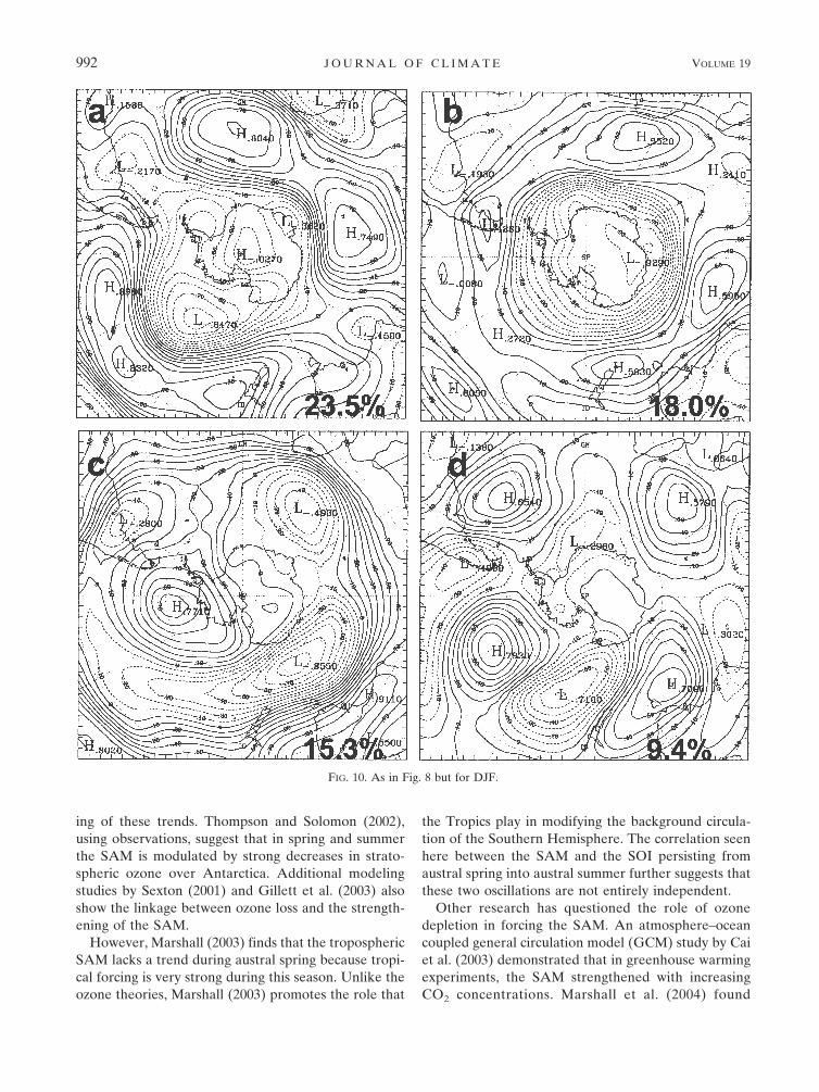
Examining the REOF patterns for this season (Fig.10) demonstrates again that the first two modes, repre-senting ENSO and the SAM, respectively, influence theheight variance in the South Pacific, especially theREOF1 pattern. Notably, the ENSO–RPC1 pattern issignificantly correlated with both the SAM and the SOIin the 1980s (Table 2), while in the 1990s the SAM issignificantly correlated with both the ENSO–RPC1 pat-tern and the more zonally symmetric structure in SAM–RPC2. The changes in the correlations of the SAMindex between the two RPC time series suggest changesin the structure of the SAM between the two decades,perhaps due to the marked strengthening of the SAMduring the 1990s in DJF (Marshall 2003).

Similar to the analysis for SON, the DJF ERA-40500-hPa geopotential height anomalies were averagedin the region 55°–65°S, 150°–120°W (labeled “DJF box80s” in Fig. 2), the area of strongest correlation seen inthe 1980s DJF (Fig. 4a). Notably, this region corre-sponds with the loading center in the South Pacific fromthe ENSO–REOF1 pattern (Fig. 10a). The anomaliesfrom this region are plotted along with the SOI andSAM in Fig. 11a. During the 1980s, it is clear that theheight anomalies respond to fluctuations in both theSOI and the SAM, giving physical meaning to the sig-nificant correlation of SAM and SOI with the RPC1time series and suggesting that these two modes work-ing together amplify the anomaly response. The nega-tive correlations persist into the 1990s, but drop belowthe 95% significance level, as the overall pattern shifts

away from this region (Fig. 4b). To account for thissouth and eastward shift, ERA-40 500-hPa geopotentialheight anomalies were averaged in the region 65°–75°S,60°–150°W (labeled “DJF box 90s” in Fig. 2) as beforeand are presented in Fig. 11b. From the time series inFig. 11b, it can be seen that the height anomalies aresignificantly correlated with both the SOI and the SAMin the 1990s, again supporting the finding that the re-gion where the ENSO teleconnection in the South Pa-cific appears strongest is governed by coupling with theSAM forcing.

The south and east shifting seen in the DJF correla-tion plots (Fig. 4) and the DJF composites (Figs. 5c and5d) from the 1980s to the 1990s is brought about notonly by the aforementioned changes in the spatial rep-resentation of the SAM, but also from the intereventvariability in ENSO. Changes in the SAM from the1980s to the 1990s explain the southward shift; theREOF2 pattern (Fig. 10b) associated with the RPC2time series confines the height anomalies closer to theAntarctic continent than the REOF1 pattern (Fig. 10a).Similarly, the eastward shift between the two decades isexplained by the strong ENSO events in the late 1990sin this season, which produced an amplified PSA2(REOF3, Fig. 10c) pattern during the austral summerseason (Bromwich et al. 2004). The PSA2–REOF3(Fig. 10c) center is located much farther east toward theAntarctic Peninsula compared to the PSA1–REOF1(Fig. 10a) center, in agreement with Mo and Peagle(2001). Thus, the strong ENSO events in the late 1990saustral summer and the changing SAM pattern duringthis season shift the annual mean teleconnection (Fig.1b) and DJF teleconnection (Fig. 4b).

The SAM–ENSO coupling is again seen in the DJFENSO composites for both the 1980s and the 1990s(Figs. 5c and 5d). Both decades show a SAM signature;the statistically significant height anomaly in the SouthPacific has the same sign as the height anomalies overthe Antarctic continent, and there are zonally symmet-ric anomalies of the opposite sign in the midlatitudes.Notably, the 1990s (Fig. 5d) show a very strong SAMpattern with an increased area of statistical significancetightly confined to the continent, in agreement withthe marked strengthening during this decade and sea-son; this is also in agreement with the stronger corre-lation of the SAM with the RPC2 time series in the1990s (Table 2).

c. Extension to previous knowledge on decadalENSO variability, 1980–2000

The results presented here indicate that the signifi-cant correlation between ENSO and the SAM createheight anomalies that amplify the ENSO response in

TABLE 2. SON and DJF ERA-40 RPC correlations with theSOI and the SAM for the 1980s and 1990s: asterisks indicatesignificance at �95% level; boldface at �99% level.

Timeseries Decade

SON DJF

SOI SAM SOI SAM

RPC1 1980s 0.16 �0.88 0.66* 0.861990s �0.50 �0.75* 0.57 0.66*

RPC2 1980s 0.79 �0.11 0.56 0.591990s 0.83 0.74* 0.39 0.64*

RPC3 1980s �0.88 �0.12 �0.40 �0.051990s �0.16 0.35 �0.39 0.19


the South Pacific and Amundsen–Bellingshausen Seas.This finding is important as it explains much of thedecadal ENSO variability with the West Antarctic pre-cipitation minus evaporation (P � E) time series seenin previous studies (e.g., Cullather et al. 1996; Brom-wich et al. 2000; Genthon and Cosme 2003). In light ofthe findings here, the persistence of a circulationanomaly during the times of strong SAM–ENSO cor-relation leads to an increased (decreased) moisture fluxonto West Antarctica during ENSO warm (cold)events. As seen in the current study, the SAM–ENSO

correlation has notable decadal changes and this, inturn, governs the large changes in the correlation be-tween the 1980s and 1990s in the West Antarctic P � Etime series and the SOI.

5. Discussion

Observations (Marshall 2003) and statistical studies(Thompson et al. 2000) have displayed large trends inthe SAM in austral summer and autumn, and thereforemany theories have been proposed regarding the forc-

FIG. 9. As in Fig. 8 but constructed using the NCEP–NCAR reanalysis.


ing of these trends. Thompson and Solomon (2002),using observations, suggest that in spring and summerthe SAM is modulated by strong decreases in strato-spheric ozone over Antarctica. Additional modelingstudies by Sexton (2001) and Gillett et al. (2003) alsoshow the linkage between ozone loss and the strength-ening of the SAM.

However, Marshall (2003) finds that the troposphericSAM lacks a trend during austral spring because tropi-cal forcing is very strong during this season. Unlike theozone theories, Marshall (2003) promotes the role that

the Tropics play in modifying the background circula-tion of the Southern Hemisphere. The correlation seenhere between the SAM and the SOI persisting fromaustral spring into austral summer further suggests thatthese two oscillations are not entirely independent.

Other research has questioned the role of ozonedepletion in forcing the SAM. An atmosphere–oceancoupled general circulation model (GCM) study by Caiet al. (2003) demonstrated that in greenhouse warmingexperiments, the SAM strengthened with increasingCO2 concentrations. Marshall et al. (2004) found

FIG. 10. As in Fig. 8 but for DJF.


through a coupled GCM run that trends in the SAMbegin prior to any observed decreases in the strato-spheric ozone. Their study concludes that the trendsresult from a combination of anthropogenic forcing (bygreenhouse gases) and natural climate variability. In astudy by Jones and Widmann (2004), a SAM recon-struction based upon sea level pressure observationsfrom 1905 to 2000 shows strong positive and negativetrends in the middle of the record that do not match anytrends in stratospheric ozone or greenhouse gases.

Thus, they claim that natural forcing factors, such assolar and volcanic variability, and internal processes inthe climate system can strongly influence the variabilityin the SAM.

There is also some support for the SAM being modu-lated by tropical SSTs. Mo (2000) regressed the scoresfrom her EOF1 (which represented SAM) on SSTs andfound that the SAM is linearly related to the tropicalSSTs, similar to the correlation seen here between theSAM and the SOI. To examine the decadal variability

FIG. 11. DJF ERA-40 500-hPa box-averaged geopotential height anomalies averaged in the region(a) 55°–65°S, 150°–120°W and (b) 65°–75°S, 150°–60°W vs the DJF SOI and SAM. Boldface corre-lations are significant at �99% level; asterisks denote correlations significant at �95% level.


in this relationship, the SON SAM was regressed ontothe SON SST anomalies between 45°S and 45°N in asimilar manner to Mo (2000). The regression coeffi-cients were then multiplied by the change in SST ateach grid point to represent the changes in SAM ex-plained by the SST changes. The SST data were ob-tained from the National Oceanic and AtmosphericAdministration (NOAA) extended reconstructed Reyn-old’s SST dataset made available by the Climate Diag-nostics Center (CDC, available online at http://www.cdc.noaa.gov/cdc/data.noaa.ersst.html). The changessignificant at �95% confidence level are displayed inFig. 12a for the whole time series and for the two de-cades individually (Figs. 12b,c). The overall results (Fig.12a) do not demonstrate any large areas where changesin the SST are related to changes in the SAM, a findingthat also exists during the 1980s (Fig. 12b). This is ex-pected and verifies the fact that no significant SAMevents occurred with the significant ENSO events dur-ing this decade in SON. The 1990s (Fig. 12c), however,

are much different in that there is a strong and signifi-cant relationship (�95% level) between the SAM andthe tropical and subtropical Pacific SST anomalies thatextend into the eastern tropical Indian Ocean, unlikethat seen in the previous decade. Interestingly, thechanges in Fig. 12c are spatially arranged in a promi-nent horseshoe pattern similar to the SSTs anomaliesseen during a La Niña event. Notably, during the 1990s(Fig. 12c) the southern branch of the horseshoe patternis well marked. Terray and Dominiak (2005) relate thissouthern branch of the SST horseshoe pattern to theenhanced upper-level convergence brought about bythe modulation of the regional meridional Hadley cir-culation. This upper-level convergence is associatedwith an upper-level low, which acts as a Rossby wavesource region for the associated PSA pattern. From Fig.12c, the negative (positive) changes in the equatorialand subtropical (western) Pacific suggests a weakeningof the SAM during times of warm (cold) SSTs in thisregion (i.e., El Niño conditions), in agreement with the

FIG. 12. SON SAM changes associated with SON SST variations from 45°S to 45°N for (a)1979–99, (b) 1980–89, and (c) 1990–99. Contour interval is one standardized unit of the SAM;only the changes significant at �95% confidence interval are plotted. Changes are calculatedby multiplying the slope of the linear regression of the SAM onto the SST anomalies by thechange in SST.


positive correlation between the SAM and the SOI inthe 1990s. Terray and Dominiak (2005) demonstrate areduction in speed of the polar front jet in the SouthPacific associated with the ENSO SST anomalies thatalso confirms the link between the ENSO and theSAM.

L’Heureux and Thompson (2006) also use regressionanalysis to examine the SAM–ENSO coupling for1979–2004. Their study demonstrates that both oscilla-tions are significantly related to the strength of the zon-ally averaged zonal wind in the high southern latitudesduring austral summer. However, they do not examinethe decadal variability in this relationship. An exten-sion of their analysis (not shown) by decade reveals thatthe strong summer relationships seen during 1979–2004masks the decadal variability presented in this paper.Notably, the significant relationship between ENSOand the zonally averaged zonal wind shifts from mid-summer (January) during the 1980s to late fall–earlysummer (October–December), in agreement with thestrong decadal variability of the SAM–ENSO relation-ship in spring and the persistence of this relationshipthrough both decades during the summer seen here.Indeed, L’Heureux and Thompson (2006) find a signifi-cant correlation between ENSO and the SAM from1979 to 2004 during austral summer.

Although the regression analyses do not explicitlyshow a cause and effect relationship of the tropical forc-ing on the high-latitude circulation due to the simulta-neous correlation of the SOI and SAM, they do clearlydemonstrate the decadal variability in this linear rela-tionship. Partial correlation analyses do not show anyconnections of the SAM with the tropical Pacific SSTs;however, this statistical method only examines the lin-ear connection with the residual variability after thecross correlation is removed. Because of the strong co-variance between these two time series, the residualpart of the SAM not explained by the SOI is small, andis also unlikely to depict the actual physical variabilityin the SAM.

Recently, a modeling study conducted using version2 of the NCAR Community Atmosphere Model(CAM2) model confirmed the tropical SST forcing ofthe SAM (i.e., Zhou and Yu 2004). They also noted asignificant relationship between the SAM and tropicalPacific SSTs in austral summer, where warm tropicalPacific SSTs lead to negative phases of the SAM, givingfurther credence to the significant positive correlationseen here between the SOI (�0 when Pacific SSTs arewarm) and SAM during this season.

Thus, an increasing body of literature points towardlarge trends in the SAM being explained not solely by

ozone depletion, but also by anthropogenic and naturalclimate variability, including the variability in the tropi-cal Pacific SSTs. In light of the fact that the ENSOfrequency and magnitude have been increasing in thelast 50 years (Diaz et al. 2001) and were particularlymarked in the 1990s with four El Niño events and twoLa Niña events (see online at http://www.cpc.ncep.noaa.gov/products/analysis_monitoring/ensostuff/ensoyears.shtml), it is not surprising to see the signifi-cant correlations between ENSO and the SAM occur-ring primarily in the 1990s and only during seasonswhen ENSO activity is particularly strong.

Although the concept of the tropical SSTs forcing theSAM may be questioned in the SH, similar connectionshave been established in the NH. Hoerling et al. (2001)using both observations and an atmospheric general cir-culation model (AGCM) show that the North AtlanticOscillation (NAO), which is alternatively termed theArctic Oscillation or Northern Annular Mode (e.g.,Thompson and Wallace 2000), is related to tropicalSSTs in both the Pacific and Indian Oceans. Their studyargues that the observed boreal winter trend in theNAO is intimately linked with the warming in the tropi-cal SSTs, suggesting that the SSTs are forcing the NHextratropical climate. Their earlier work was later up-dated by more modeling experiments where they fur-ther conclude that the tropical Indian Ocean SSTs sig-nificantly modulate the NAO (Hurrell et al. 2004;Hoerling et al. 2004).

The exact mechanism controlling the coupling needsfurther study, and many questions remain unanswered.Examining the role of the meridional circulation acrossthe Southern Hemisphere in relation to the SAM andENSO variability might help to unlock some of theseanswers. Additional modeling work, both regionallyand globally, can help to demonstrate nonlinear com-ponents that lead to the coupling, especially sinceHoerling et al. (2004) find that the NAO is stronglymodulated by nonlinear atmospheric processes arisingfrom the increasing tropical Indian Ocean SSTs.

6. Summary

Decadal variability of the ENSO teleconnection inthe South Pacific has been presented. This decadal vari-ability is observed in many fields including the annualmean MSLP and the 500-hPa geopotential height. An-nual mean upper-level wind and MSLP observationsare also used to demonstrate the decadal variability andsupport the spatial representations produced by theERA-40 reanalysis used in the study. Results in these


annual mean fields indicate a weak teleconnection inthe 1980s in a small region in the South Pacific followedby a strong response during the 1990s across nearly theentire South Pacifc and Amundsen–BellingshausenSeas.

Examining the decadal variability demonstrates thatthe strong ENSO teleconnection seen in the annualmean plots is accounted for by the teleconnections dur-ing SON and DJF. The reduced annual teleconnectionduring the 1980s is readily explained by the lack ofresponse during SON in the 1980s; during DJF the tele-connection remains strong for both the 1980s and the1990s although its spatial representation is different.ENSO composites that concentrate on these seasonsconfirm the decadal variability seen in the correlationplots. Previous studies have not observed the decadalvariability as they have averaged over a time interval ofmore than one decade and only examined connectionsduring austral winter, a season for which no significantcorrelation was found in the current study.

Through empirical orthogonal function analysis itwas found that the patterns correlated with the ENSOand SAM have large loading centers in the South Pa-cific. As such, the high southern latitude ENSO tele-connection is amplified in the South Pacific duringtimes when the SAM is positively correlated with theSOI, and can be weakened during times of insignificantor negative correlation. The connections between theENSO and SAM appear only in the seasons when theENSO forcing is particularly strong, namely, australspring and summer.

The results presented here, in combination with agrowing body of literature, suggest that tropical ENSOactivity plays an important role in the forcing of thehigh southern latitude tropospheric circulation. It is un-clear whether the coupling observed here between thehigh-latitude SH circulation and ENSO is part of natu-ral climate variability or climate change; the quality ofthe available reanalyses limits the study to roughly thelast two decades. However, the associations depicted inthe 1990s are the strongest observed during this timeperiod, in agreement with other recent studies (e.g.,Bromwich et al. 2004).

Acknowledgments. The authors thank Zhichang Guofor the original design of the program used in calculat-ing the correlations with the SOI, Sheng-Hung Wangfor EOF assistance, and Jorge Carrasco for supplyingthe 500-hPa zonal wind data for Punta Arenas. Com-ments from two anonymous reviewers helped to clarifyand strengthen the manuscript. Discussions with DavidThompson are appreciated and also helped to improvethe paper. This research was funded in part by NSF

Grant OPP-0337948 and UCAR Subcontract SO1-22961.

REFERENCES

Bell, G. D., and M. S. Halpert, 1998: Climate assessment for 1997.Bull. Amer. Meteor. Soc., 79, S1–S50.

——, and Coauthors, 2000: Climate assessment for 1999. Bull.Amer. Meteor. Soc., 81, S1–S50.

Bromwich, D. H., and R. L. Fogt, 2004: Strong trends in the skillof the ERA-40 and NCEP–NCAR reanalyses in the high andmiddle latitudes of the Southern Hemisphere, 1958–2001. J.Climate, 17, 4603–4619.

——, A. N. Rogers, P. Kallberg, R. I. Cullather, J. W. C. White,and K. J. Kreutz, 2000: ECMWF analyses and reanalyses de-piction of ENSO signal in Antarctic precipitation. J. Climate,13, 1406–1420.

——, A. J. Monaghan, and Z. Guo, 2004: Modeling the ENSOmodulation of Antarctic climate in the late 1990s with PolarMM5. J. Climate, 17, 109–132.

Cai, W. J., P. H. Whetton, and D. J. Karoly, 2003: The response ofthe Antarctic Oscillation to increasing and stabilized atmo-spheric CO2. J. Climate, 16, 1525–1538.

Cullather, R. I., D. H. Bromwich, and M. L. van Woert, 1996: In-terannual variations in Antarctic precipitation related to ElNiño–Southern Oscillation. J. Geophys. Res., 101, 19 109–19 118.

Diaz, H. F., M. P. Hoerling, and J. K. Eischeid, 2001: ENSO vari-ability, teleconnections and climate change. Int. J. Climatol.,21, 1845–1862.

Genthon, C., and E. Cosme, 2003: Intermittent signature ofENSO in west-Antarctic precipitation. Geophys. Res. Lett.,30, 2081, doi:10.1029/2003GL018280.

——, G. Krinner, and M. Sacchettini, 2003: Interannual Antarctictropospheric circulation and precipitation variability. ClimateDyn., 21, 289–307.

Gillett, N. P., M. R. Allen, and K. D. Williams, 2003: Modellingthe atmospheric response to doubled CO2 and depletedstratospheric ozone using a stratosphere-resolving coupledGCM. Quart. J. Roy. Meteor. Soc., 129, 947–966.

Gong, D., and S. Wang, 1999: Definition of Antarctic oscillationindex. Geophys. Res. Lett., 26, 459–462.

Guo, Z., D. H. Bromwich, and K. M. Hines, 2004: Modeled Ant-arctic precipitation. Part II: ENSO modulation over WestAntarctica. J. Climate, 17, 448–465.

Harangozo, S. A., 2000: A search for ENSO teleconnections in theWest Antarctic Peninsula climate in austral winter. Int. J.Climatol., 20, 663–679.

Hoerling, M. P., J. W. Hurrell, and T. Xu, 2001: Tropical originsfor recent North Atlantic climate change. Science, 292, 90–92.

——, ——, ——, G. T. Bates, and A. S. Phillips, 2004: Twentiethcentury North Atlantic climate change. Part II: Understand-ing the effect of Indian Ocean warming. Climate Dyn., 23,391–405.

Houseago, R., G. R. McGregor, J. C. King, and S. A. Harangozo,1998: Climate anomaly wave train patterns linking southernlow and high latitudes during South Pacific warm and coldevents. Int. J. Climatol., 20, 793–801.

Hurrell, J. W., M. P. Hoerling, A. S. Phillips, and T. Xu, 2004:Twentieth century North Atlantic climate change. Part I: As-sessing determinism. Climate Dyn., 23, 371–389.

Jones, J. M., and M. Widmann, 2004: Atmospheric science—Earlypeak in Antarctic oscillation index. Nature, 432, 290–291.


Karoly, D. J., 1989: Southern Hemisphere circulation features as-sociated with El Niño–Southern Oscillation events. J. Cli-mate, 2, 1239–1252.

——, P. Hope, and P. D. Jones, 1996: Decadal variations of theSouthern Hemisphere circulation. Int. J. Climatol., 16, 723–738.

Kiladis, G. N., and K. C. Mo, 1998: Interannual and intraseasonalvariability in the Southern Hemisphere. Meteorology of theSouthern Hemisphere, D. J. Karoly and D. G. Vincent, Eds.,Amer. Meteor. Soc., 307–336.

Kwok, R., and J. C. Comiso, 2002: Southern Ocean climate andsea ice anomalies associated with the Southern Oscillation. J.Climate, 15, 487–501.

L’Heureux, M. L., and D. W. J. Thompson, 2006: Observed rela-tionships between the El Niño–Southern Oscillation and theextratropical zonal-mean circulation. J. Climate, 19, 276–287.

Marshall, G. J., 2003: Trends in the Southern Annular Mode fromobservations and reanalyses. J. Climate, 16, 4134–4143.

——, P. A. Stott, J. Turner, W. M. Connolley, J. C. King, andT. A. Lachlan-Cope, 2004: Causes of exceptional atmo-spheric circulation changes in the Southern Hemisphere.Geophys. Res. Lett., 31, L14205, doi:10.1029/2004GL019952.

Mo, K. C., 2000: Relationships between low-frequency variabilityin the Southern Hemisphere and sea surface temperatureanomalies. J. Climate, 13, 3599–3610.

——, and M. Ghil, 1987: Statistics and dynamics of persistentanomalies. J. Atmos. Sci., 44, 877–901.

——, and W. Higgins, 1998: The Pacific–South American modesand tropical convection during the Southern Hemispherewinter. Mon. Wea. Rev., 126, 1581–1596.

——, and J. N. Peagle, 2001: The Pacific–South American modesand their downstream effects. Int. J. Climatol., 21, 1211–1229.

North, G. R., T. L. Bell, R. F. Cahalan, and F. J. Moeng, 1982:Sampling errors in the estimation of empirical orthogonalfunctions. Mon. Wea. Rev., 110, 699–706.

Renwick, J. A., 1998: ENSO-related variability in the frequency ofSouth Pacific blocking. Mon. Wea. Rev., 126, 3117–3123.

——, and M. J. Revell, 1999: Blocking over the South Pacific andRossby wave propagation. Mon. Wea. Rev., 127, 2233–2247.

Revell, M. J., J. W. Kidson, and G. N. Kiladis, 2001: Interpretinglow-frequency modes of Southern Hemisphere atmosphericvariability as the rotational response to divergent forcing.Mon. Wea. Rev., 129, 2416–2425.

Richman, M. B., 1986: Rotation of principal components. J. Cli-matol., 6, 293–335.

Rogers, J. C., and H. van Loon, 1982: Spatial variability of sealevel pressure and 500-mb height anomalies over the South-ern Hemisphere. Mon. Wea. Rev., 110, 1375–1392.

Sexton, D. M. H., 2001: The effect of stratospheric ozone deple-tion on the phase of the Antarctic Oscillation. Geophys. Res.Lett., 28, 3697–3700.

Silvestri, G. E., and C. S. Vera, 2003: Antarctic Oscillation signalon precipitation anomalies over southeastern South America.Geophys. Res. Lett., 30, 2115, doi:10.1029/2003GL018277.

Sterl, A., 2004: On the (in)homogeneity of reanalysis products. J.Climate, 17, 3866–3873.

Terray, P., and S. Dominiak, 2005: Indian Ocean sea surface tem-peratures and El Niño–Southern Oscillation: A new perspec-tive. J. Climate, 18, 1351–1368.

Thompson, D. W., and J. M. Wallace, 2000: Annular modes in theextratropical circulation. Part I: Month-to-month variability.J. Climate, 13, 1000–1016.

——, and S. Solomon, 2002: Interpretation of recent SouthernHemisphere climate change. Science, 296, 895–899.

——, and D. J. Lorenz, 2004: The signature of the annular modesin the tropical troposphere. J. Climate, 17, 4330–4342.

——, J. M. Wallace, and G. C. Hegerl, 2000: Annular modes in theextratropical circulation. Part II: Trends. J. Climate, 13, 1018–1036.

Trenberth, K. E., 1997: The definition of El Niño. Bull. Amer.Meteor. Soc., 78, 2771–2777.

——, and J. M. Caron, 2000: The Southern Oscillation revisited:Sea level pressures, surface temperatures, and precipitation.J. Climate, 13, 4358–4365.

——, D. P. Stepaniak, and L. Smith, 2005: Interannual variabilityof patterns of atmospheric mass distribution. J. Climate, 18,2812–2825.

Turner, J., 2004: Review: The El Niño-Southern Oscillation andAntarctica. Int. J. Climatol., 24, 1–31.

van Loon, H., and D. J. Shea, 1987: The Southern Oscillation. PartVI: Anomalies of sea level pressure on the Southern Hemi-sphere and of Pacific sea surface temperature during the de-velopment of a warm event. Mon. Wea. Rev., 115, 370–379.

Wallace, J. M., and D. S. Gutzler, 1981: Teleconnection in thegeopotential height field during the Northern Hemispherewinter. Mon. Wea. Rev., 109, 784–812.

Zhou, T. and R. Yu, 2004: Sea-surface temperature induced vari-ability of the Southern Annular Mode in an atmospheric gen-eral circulation model. Geophys. Res. Lett., 31, L24206,doi:10.1029/2004GL021473.


Decadal Variability of the ENSO Teleconnection to the...

Documents

Transcript of Decadal Variability of the ENSO Teleconnection to the...