A Teleconnection between the West Siberian Plain and the ENSO Region

STEFAN LIESS

Department of Earth Sciences, University of Minnesota, Minneapolis, Minnesota

SAURABH AGRAWAL

Department of Computer Science and Engineering, University of Minnesota, Minneapolis, Minnesota

SNIGDHANSU CHATTERJEE

Department of Statistics, University of Minnesota, Minneapolis, Minnesota

VIPIN KUMAR

Department of Computer Science and Engineering, University of Minnesota, Minneapolis, Minnesota

(Manuscript received 14 December 2015, in final form 21 July 2016)

ABSTRACT

TheWalker circulation is linked to extratropical waves that are deflected from theNorthernHemisphere polarregions and travel southeastward over central Asia toward the western Pacific warm pool during northern winter.The wave pattern resembles the east Atlantic–west Russia pattern and influences the El Niño–Southern Oscil-lation (ENSO) region. A tripole pattern between theWest Siberian Plain and the two centers of action of ENSOindicates that the background state of ENSO with respect to global sea level pressure (SLP) has a significantnegative correlation to theWest Siberian Plain. The correlationwith the background state, which is defined by thesumof the two centers of action of ENSO, is higher than eachof the pairwise correlationswith either of theENSOcenters alone. The centers are defined with a clustering algorithm that detects regions with similar characteristics.The normalizedmonthly SLP time series for the two centers of ENSO (aroundDarwin, Australia, and Tahiti) arearea averaged, and the sumof both regions is considered as the background state of ENSO.This wave train can bedetected throughout the troposphere and the lower stratosphere. Its origins can be traced back to Rossby waveactivity triggered by convection over the subtropical North Atlantic that emanates wave activity toward theWestSiberian Plain. The samewave train also propagates to the central PacificOcean aroundTahiti and can be used topredict the background state over the ENSO region. This background state also modifies the subtropical bridgebetween tropical eastern Pacific and subtropical North Atlantic leading to a circumglobal wave train.

1. Introduction

Interannual variations of the climate over the tropicalPacific are dominated by El Niño–Southern Oscillation(ENSO) and the low-frequency variability of ENSO isoften attributed to the Pacific decadal oscillation(PDO). El Niño (La Niña) patterns are stronger and

more consistent during the positive (negative) phase ofthe PDO (Gershunov and Barnett 1998). The empiricalorthogonal function (EOF) calculation for the PDO in-dex is restricted to the North Pacific (208–708N), but thespatial pattern of sea surface temperature (SST) anom-alies associated with the PDO is similar to that associatedwithENSO (Deser et al. 2010, their Fig. 10) except for therelative weighting between the northern and tropicalPacific. The amplitudes of the SST anomalies in theequatorial eastern Pacific for the PDO are comparablewith those in the North Pacific but they are weaker thanthe ENSO signal (Zhang et al. 1997; Dettinger et al. 2000;Deser et al. 2004, 2010).The PDO is stronger influencing the eastern part of

the Walker circulation over the central and eastern

Supplemental information related to this paper is available at theJournals Online website: http://dx.doi.org/10.1175/JCLI-D-15-0884.s1.

Corresponding author address: Stefan Liess, Departmentof Earth Sciences, University of Minnesota, 310 PillsburyDr., Minneapolis, MN 55455.E-mail: liess@umn.edu

1 JANUARY 2017 L I E S S ET AL . 301

DOI: 10.1175/JCLI-D-15-0884.1

! 2017 American Meteorological Society

Pacific (Gershunov and Barnett 1998; Verdon andFranks 2006; Deser et al. 2010) than the western part. Asimilar relationship exists between the Walker circula-tion and the North Pacific Gyre Oscillation (Chhak et al.2009; Di Lorenzo et al. 2010), which is predominantly anocean response to large-scale atmospheric forcing overthe North Pacific. An anomalous lower-troposphericanticyclone (cyclone) located in the western North Pa-cific bridges the warm (cold) ENSOevents in the easternPacific and the weak (strong) East Asian winter mon-soon (EAWM) (Wang et al. 2000). However, Wanget al. (2008) point out that the phase of the PDO shouldbe taken into account in the ENSO-based prediction ofwintertime climate over East Asia. The ENSO impacton the EAWM is stronger when the PDO is in its neg-ative phase. Also, rainfall and crop yields over Australiaare more predictable during the negative PDO period(Power et al. 1999). However, interannual hydroclimatevariations in central Asia are more significant during thepositive PDOphase (Fang et al. 2014). Thus, the PDOcanbe described as a background state for decadal ENSOvariability such as the recent shift from low-frequencyeastern Pacific El Niño events toward higher-frequencycentral Pacific El Niño events (Kim et al. 2009; Kuget al. 2009; Xie et al. 2015).ENSO-related eastward propagating Rossby waves

produce generally wetter (drier) conditions over NorthAmerica during El Niño (La Niña) events (Ropelewskiand Halpert 1986; Trenberth and Guillemot 1996), butmore refined results can be obtained by taking spatialENSO characteristics into account (Larkin and Harrison2005) and investigating the combined effect of ENSO andthe Pacific–North American (PNA) pattern (Garfinkeland Hartmann 2008). Similarly, although El Niño eventsare generally accompanied by negative North AtlanticOscillation (NAO) periods (Gouirand and Moron 2003;Brönnimann et al. 2007), this relationship ismostly true forEl Niño events with maximum SST anomalies over thecentral Pacific, whereas El Niño events with maximumSSTanomalies over the easternPacific can even contributeto positive NAO periods (Graf and Zanchettin 2012).Traditionally, the stationary patterns in wave trains

that encompass planetary-scale regions have been de-scribed as teleconnections (e.g., Wallace and Gutzler1981; Barnston and Livezey 1987). These teleconnectionswith frequencies of 10–60 days are often identified asmain contributors to blocking patterns. For example,during boreal summer 2010, a strong eastern Europeanblocking and its quasi-stationary wave structure wassupported by a combination of a La Niña event and anenhanced polar Arctic dipole mode (Schneidereit et al.2012). Wave trains that commenced over both the NorthPacific and North Atlantic propagated toward eastern

Europe and the polar region, and continued southeastwardtoward South Asia (Schneidereit et al. 2012). The latter isthe east Atlantic–west Russia (EA–WR) pattern (Krichakand Alpert 2005) that was originally referred to as theEurasia-2 pattern (Barnston and Livezey 1987). Itsplanetary-scale impacts can even be related to vege-tation productivity over the Amazon region (Gonsamoet al. 2015).Here, we introduce an SLP-based index that describes

the background state of the ENSO region and shows howthis background state is connected to the West SiberianPlain via a Rossby wave train. Similar to the PDO, thiswave train can be used to predict the atmospheric stateover the ENSO region and the preferences for the spatialdistribution of ENSO activity. However, it should benoted that the slowly evolving oceanic PDO index doesnot constrain the atmospheric variability in subsequentmonths (Kumar et al. 2013). The significance ofmean SLPanomalies over the West Siberian Plain on NorthernHemispheric climate has previously been described bySmoliak and Wallace (2015), but their analysis has notfocused on interactions with tropical climate.Section 2 of this paper introduces the statistical method

used to identify the relationship between the West Sibe-rian Plain and the ENSO region, and the physical mech-anisms that govern this relationship are described insection 3. Section 4 links this relationship to a circum-global wave pattern over the Northern Hemisphere andthe results are summarized and discussed in section 5.

2. Identification of tripole patterns

This study uses detrended multiyear monthly meananomalies of the National Centers for EnvironmentalPrediction (NCEP)–U.S. Department of Energy (DOE)Reanalysis-2 (NCEP-2) SLP data (Kanamitsu et al.2002) and alternatively the Modern-Era RetrospectiveAnalysis for Research andApplications (MERRA) SLPdata (Rienecker et al. 2011) for December–February(DJF) during 1979–2014. MERRA SLP data were in-terpolated to the 2.58 3 2.58 horizontal resolution ofNCEP-2 and both datasets were normalized by dividingSLP over each grid point with its respective temporalstandard deviation. This normalization reduces thestronger SLP variability over high and midlatitudescompared to low latitudes. The SLP data have beendetrended to reduce the influence of multidecadal os-cillations and long-term climate change, which are un-likely initiated by atmospheric Rossby wave activity.Positive long-term SLP trends over the West SiberianPlain and negative trends over eastern Europe andeastern Canada would have contributed to negativecorrelations (Simmonds 2015, his Fig. 7). Long-term

302 JOURNAL OF CL IMATE VOLUME 30

SLP trends over the equatorial region are much lower(Gillett and Stott 2009, their Fig. 1).In this study, we define tripole patterns as patterns

that comprise of three regions R1, R2, and R3 with theircorresponding normalized and area-averaged SLP timeseries denoted by T1, T2, and T3 respectively, such thatT3 shows a stronger correlation with T11 T2 comparedto the correlations between T1 and T3 and between T2and T3. As a result, a tripole captures a relationshipbetween R3 and the area comprising the combined re-gions R1 and R2, which is stronger than the two indi-vidual relationships between R3 and R1 and betweenR3 and R2. The strength of a tripole is measured as thecorrelation between T1 1 T2 and T3. For normalizedtime series where all the three pairwise correlationsbetween R1, R2, and R3 are negative, the combinedcorrelation can be directly computed using the followingrelation:

corr(T11T2, T3)5corr(T1, T3)1 corr(T2, T3)ffiffiffiffiffiffiffiffiffiffiffiffiffiffiffiffiffiffiffiffiffiffiffiffiffiffiffiffiffiffiffiffiffiffiffiffiffiffiffiffi

2[11 corr(T1, T2)]p . (1)

As seen in Eq. (1), the negative correlation, or strength,of a tripole increases as the absolute values of each of thethree pairwise negative correlations increases. A detailedproof is discussed in the appendix.To detect negative tripoles, we use a graph-based

approach (Kawale et al. 2011, 2013; Liess et al. 2014)that has been used to identify pairs of negatively cor-related regions. Such pairs can be found by graph-basedmethods without requiring a priori region selection orimposing an orthogonality constraint, as in singularvalue decomposition (SVD) or EOF analysis (Newmanand Sardeshmukh 1995; Dommenget and Latif 2002).Our method to find tripoles consists of two steps. In

the first step, pairs of negatively correlated regions arefound, and in the second step, we search for all the re-gions that show a negative correlation with both ends ofthe initial pair of regions.Within a global SLP dataset, first all pairs of grid

points that are strongly negatively correlated with eachother are identified as initial centers of the regions R1and R2. R1 and R2 are then constructed such that allgrid points in R1 and R2 show 1) a positive correlation of0.85 or larger with their corresponding centers and 2) anegative correlation of 20.3 or lower with at least oneof the grid points in the opposite region.In the second step, for each pair (R1, R2) found

above, grid points that are most negatively correlatedwith a grid point in either of the two regions R1 or R2are used as centers for regions R3. R3 contains gridpoints that have 1) a positive correlation of 0.85 or largerwith their center and 2) a negative correlation of 20.15

or lower with at least one of the grid points in eitherregion R1 or R2. All the grid points included in R3 arethen excluded from being selected as centers of sub-sequent regions and step 2 is repeated to obtain multiplecandidates for R3. Only those triplets of regions R1, R2,and R3 are considered as tripoles where 1) the correla-tion between R11 R2 and R3 is statistically significant,2) a substantial improvement exists in the strength ofcorrelation between R1 1 R2 and R3 compared to R1and R3 and to R2 and R3, respectively, and 3) each ofthe three regions consists of at least 40 grid points. In theNCEP-2 SLP dataset, this algorithm identifies 124 tripolesincluding parts of the PNA pattern, but many tripoles canbe classified as either spurious or overlapping with pre-viously detected regions. If the correlation thresholdschange from 0.85 to 0.8 and from 20.15 to 20.2, the al-gorithm identifies 178 tripoles in very similar locations.The alternative regions corresponding to the index de-scribed in the next section are shown in Fig. S1a in thesupplemental material. Additional details about the al-gorithm can be found in Agrawal et al. (2015). A detaileddiscussion about the statistical significance of the corre-lation thresholds based on field significance (Wilks2006, 2016) and a multiple testing correction for thefalse discovery rate (FDR; Benjamini and Hochberg1995; Benjamini and Yekutieli 2001) is included in thesupplemental material. The algorithm was initially runon NCEP-2 SLP and the tripole patterns discoveredwere verified onMERRASLP andHadley Centre SLPdata (HadSLP2; Allan and Ansell 2006).

3. A link between the West Siberian Plain and theENSO region

Figure 1 shows three regions forming a tripole patternbetween the tropical Pacific and theWest Siberian PlainduringDJF. The background state of ENSO is describedby the normalized and area-averaged SLP values over aregion in the western Pacific warm pool (green), here-after named R1, and a region in the central Pacific justsouth of where the Niño-3.4 and Niño-4 regions overlap(cyan), hereafter named R2. It should be noted that al-though we identify a tripole pattern, we combine regionsR1 and R2 to show their combined relation to the WestSiberian Plain (magenta), hereafter named R3. Thecombination of R1 and R2 describes a background stateover the ENSO region that contains information aboutits area-averaged SLP strength compared to the globalaverage SLP, which varies only by 0.5 hPa (Trenberth1981). Thus, our definition of a tripole pattern includes anoscillation between R1 and R2 in the Pacific basin, and anoscillation between the combined region R1 1 R2 in thePacific basin and a third region R3 outside the Pacific

1 JANUARY 2017 L I E S S ET AL . 303

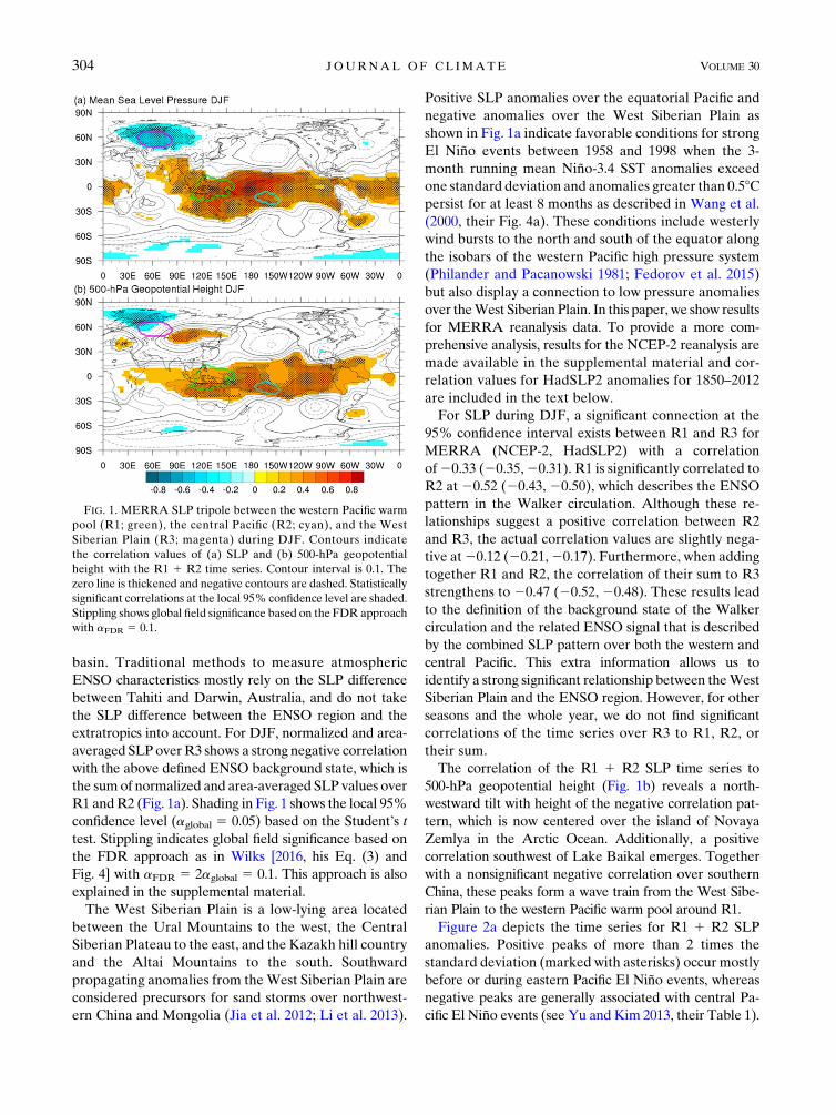
basin. Traditional methods to measure atmosphericENSO characteristics mostly rely on the SLP differencebetween Tahiti and Darwin, Australia, and do not takethe SLP difference between the ENSO region and theextratropics into account. For DJF, normalized and area-averaged SLPoverR3 shows a strong negative correlationwith the above defined ENSO background state, which isthe sumof normalized and area-averaged SLP values overR1 andR2 (Fig. 1a). Shading in Fig. 1 shows the local 95%confidence level (aglobal 5 0.05) based on the Student’s ttest. Stippling indicates global field significance based onthe FDR approach as in Wilks [2016, his Eq. (3) andFig. 4] with aFDR 5 2aglobal 5 0.1. This approach is alsoexplained in the supplemental material.The West Siberian Plain is a low-lying area located

between the Ural Mountains to the west, the CentralSiberian Plateau to the east, and the Kazakh hill countryand the Altai Mountains to the south. Southwardpropagating anomalies from theWest Siberian Plain areconsidered precursors for sand storms over northwest-ern China and Mongolia (Jia et al. 2012; Li et al. 2013).

Positive SLP anomalies over the equatorial Pacific andnegative anomalies over the West Siberian Plain asshown in Fig. 1a indicate favorable conditions for strongEl Niño events between 1958 and 1998 when the 3-month running mean Niño-3.4 SST anomalies exceedone standard deviation and anomalies greater than 0.58Cpersist for at least 8 months as described in Wang et al.(2000, their Fig. 4a). These conditions include westerlywind bursts to the north and south of the equator alongthe isobars of the western Pacific high pressure system(Philander and Pacanowski 1981; Fedorov et al. 2015)but also display a connection to low pressure anomaliesover theWest SiberianPlain. In this paper, we show resultsfor MERRA reanalysis data. To provide a more com-prehensive analysis, results for the NCEP-2 reanalysis aremade available in the supplemental material and cor-relation values for HadSLP2 anomalies for 1850–2012are included in the text below.For SLP during DJF, a significant connection at the

95% confidence interval exists between R1 and R3 forMERRA (NCEP-2, HadSLP2) with a correlationof20.33 (20.35,20.31). R1 is significantly correlated toR2 at 20.52 (20.43, 20.50), which describes the ENSOpattern in the Walker circulation. Although these re-lationships suggest a positive correlation between R2and R3, the actual correlation values are slightly nega-tive at20.12 (20.21,20.17). Furthermore, when addingtogether R1 and R2, the correlation of their sum to R3strengthens to 20.47 (20.52, 20.48). These results leadto the definition of the background state of the Walkercirculation and the related ENSO signal that is describedby the combined SLP pattern over both the western andcentral Pacific. This extra information allows us toidentify a strong significant relationship between theWestSiberian Plain and the ENSO region. However, for otherseasons and the whole year, we do not find significantcorrelations of the time series over R3 to R1, R2, ortheir sum.The correlation of the R1 1 R2 SLP time series to

500-hPa geopotential height (Fig. 1b) reveals a north-westward tilt with height of the negative correlation pat-tern, which is now centered over the island of NovayaZemlya in the Arctic Ocean. Additionally, a positivecorrelation southwest of Lake Baikal emerges. Togetherwith a nonsignificant negative correlation over southernChina, these peaks form a wave train from the West Sibe-rian Plain to the western Pacific warm pool around R1.Figure 2a depicts the time series for R1 1 R2 SLP

anomalies. Positive peaks of more than 2 times thestandard deviation (marked with asterisks) occur mostlybefore or during eastern Pacific El Niño events, whereasnegative peaks are generally associated with central Pa-cific El Niño events (see Yu and Kim 2013, their Table 1).

FIG. 1. MERRA SLP tripole between the western Pacific warmpool (R1; green), the central Pacific (R2; cyan), and the WestSiberian Plain (R3; magenta) during DJF. Contours indicatethe correlation values of (a) SLP and (b) 500-hPa geopotentialheight with the R1 1 R2 time series. Contour interval is 0.1. Thezero line is thickened and negative contours are dashed. Statisticallysignificant correlations at the local 95% confidence level are shaded.Stippling shows global field significance based on the FDR approachwith aFDR 5 0.1.

304 JOURNAL OF CL IMATE VOLUME 30

The positive peaks of more than 2 times the standarddeviation in R3 are marked with crosses. During thepositive R3 peaks of December 1984, June 1989,September 1992, November 1996, and December 2012,the related R1 1 R2 values are outside one standarddeviation. Only the June 1989 value relates to a positiveR11 R2 value. The same markers are applied to the R3time series (Fig. 2b). Since most of the R11 R2 markersdo not correspond to peaks in the R3 time series, it issuggested that the R11R2 regions do not play a big rolein the signal detected over the R3 region. In contrast,Fig. 2a suggests that positive peaks over the R3 regionmay be influencing the negative peaks over the R11 R2regions during northern fall and winter. Positive peaks ofmore than 1.5 times the standard deviation corroborate theabove result with two-thirds of the peaks in R3 occurringduring negativeR11R2phases and10 (4) peaks occurringoutside the negative (positive)R11R2 standard deviationmostly during boreal winter (summer) months (Fig. S10 inthe supplemental material).Composite maps of geopotential height fields in

Figs. 3 and 4 include the temporally averaged pattern of

all positive minus all negative monthly events outsideone standard deviation as detected in the R11 R2 timeseries in Fig. 2a. Here, we refer to these average patternsoutside one standard deviation as positive and negativephases of the wave activity. The dates that contribute tothe positive and negative phases are listed in Table S1 inthe supplemental material. Composites also display thenorthward shift of the center of action with height overthe R3 region during DJF. Regions with locally signifi-cant differences between the positive and negativephase are identified with the Student’s t test at a 95%confidence interval (shaded in Figs. 3 and 4) and globalfield significance that corrects for spatial autocorrelationis based on the FDR approach with aFDR 5 0.1 (stipp-ling in Figs. 3 and 4). The 850-hPa geopotential heightpattern during DJF in Fig. 3a resembles the SLP cor-relation pattern in Fig. 1a. The strongest negative am-plitudes occur over the West Siberian Plain and NovayaZemlya, and strong positive amplitudes occur over theR1 and R2 regions, similar to the eastern Pacific El Niñophase minus the central Pacific El Niño phase (Graf andZanchettin 2012, their Fig. 3, right panel).The composite pattern during JJA (Fig. 3b) reveals

statistically significant positive connections throughoutcentral Asia from theWest Siberian Plain to the tropicalPacific indicating a nonlinear significant relationshipthat cannot be found with linear correlation (not shown)but is corroborated by the positive relation during June1989 (see Fig. 2a). The composite pattern also shows anegative connection over the Ross Sea near Antarctica.At 500 hPa, the four peaks of the wave train are depictedduring DJF (Fig. 3c). Compared to DJF, these peaks areshifted westward during JJA starting with a negativecenter northwest of Norway, positive centers over theWest Siberian Plain and the tropical Pacific, and a smallnonsignificant negative peak over the Hindu Kush(Fig. 3d). However, there is no apparent vertical tilt in theJJA geopotential height pattern, suggesting the occur-rence of a stationary wave during this season. In general,the relationship between R1 1 R2 and R3 has a seasonaldependence that can influence the sign of its correlation.The transitional seasons of MAM and SON show similarcharacteristics to DJF, but the patterns are less significant(not shown).

4. A circumglobal wave train

Geopotential height fields in the upper troposphere andthe lower stratosphere (Fig. 4) corroborate the results ofFig. 3. Amplitudes are generally stronger at these levels(please note the different contour intervals in Figs. 3 and 4)and the tropical atmosphere is less significantly impacted.However, although Figs. 4a and 4c indicate the interplay

FIG. 2. Time series of MERRA SLP divided by its standarddeviation for (a) area averages over R1 1 R2 with asterisks in-dicating values above two standard deviations and (b) the areaaverage over R3 with crosses indicating values above two standarddeviations.Marks for each time series are shown in both time seriesfor easier comparison.Horizontal lines indicate plus andminus onestandard deviation.

1 JANUARY 2017 L I E S S ET AL . 305

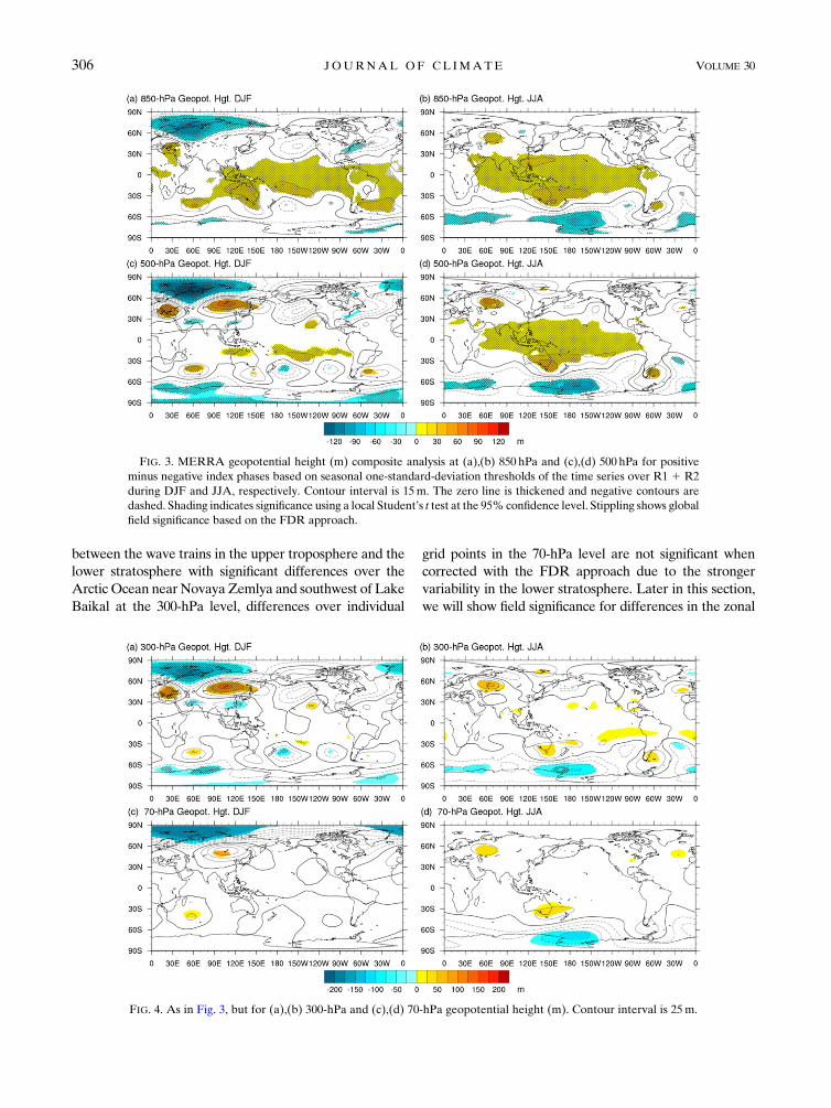
between the wave trains in the upper troposphere and thelower stratosphere with significant differences over theArctic Ocean near Novaya Zemlya and southwest of LakeBaikal at the 300-hPa level, differences over individual

grid points in the 70-hPa level are not significant whencorrected with the FDR approach due to the strongervariability in the lower stratosphere. Later in this section,we will show field significance for differences in the zonal

FIG. 3. MERRA geopotential height (m) composite analysis at (a),(b) 850 hPa and (c),(d) 500 hPa for positiveminus negative index phases based on seasonal one-standard-deviation thresholds of the time series over R1 1 R2during DJF and JJA, respectively. Contour interval is 15m. The zero line is thickened and negative contours aredashed. Shading indicates significance using a local Student’s t test at the 95% confidence level. Stippling shows globalfield significance based on the FDR approach.

FIG. 4. As in Fig. 3, but for (a),(b) 300-hPa and (c),(d) 70-hPa geopotential height (m). Contour interval is 25m.

306 JOURNAL OF CL IMATE VOLUME 30

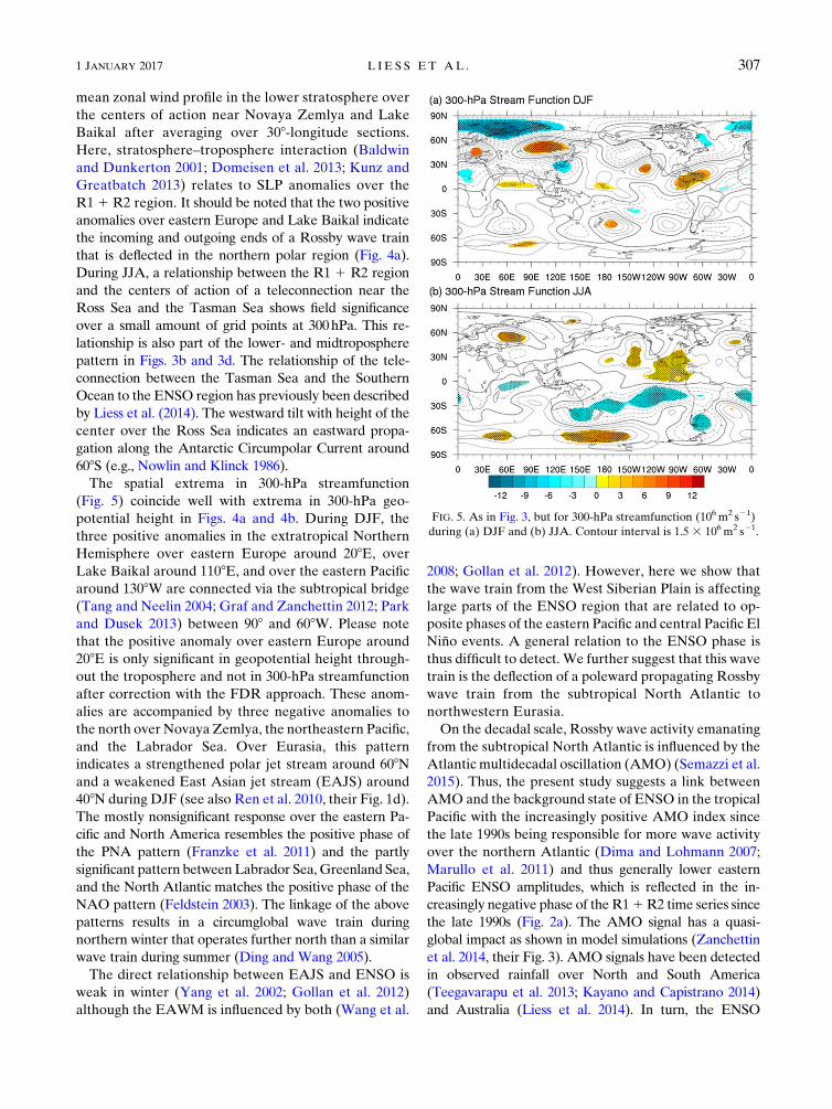
mean zonal wind profile in the lower stratosphere overthe centers of action near Novaya Zemlya and LakeBaikal after averaging over 308-longitude sections.Here, stratosphere–troposphere interaction (Baldwinand Dunkerton 2001; Domeisen et al. 2013; Kunz andGreatbatch 2013) relates to SLP anomalies over theR1 1 R2 region. It should be noted that the two positiveanomalies over eastern Europe and Lake Baikal indicatethe incoming and outgoing ends of a Rossby wave trainthat is deflected in the northern polar region (Fig. 4a).During JJA, a relationship between the R1 1 R2 regionand the centers of action of a teleconnection near theRoss Sea and the Tasman Sea shows field significanceover a small amount of grid points at 300hPa. This re-lationship is also part of the lower- and midtropospherepattern in Figs. 3b and 3d. The relationship of the tele-connection between the Tasman Sea and the SouthernOcean to the ENSO region has previously been describedby Liess et al. (2014). The westward tilt with height of thecenter over the Ross Sea indicates an eastward propa-gation along the Antarctic Circumpolar Current around608S (e.g., Nowlin and Klinck 1986).The spatial extrema in 300-hPa streamfunction

(Fig. 5) coincide well with extrema in 300-hPa geo-potential height in Figs. 4a and 4b. During DJF, thethree positive anomalies in the extratropical NorthernHemisphere over eastern Europe around 208E, overLake Baikal around 1108E, and over the eastern Pacificaround 1308W are connected via the subtropical bridge(Tang and Neelin 2004; Graf and Zanchettin 2012; Parkand Dusek 2013) between 908 and 608W. Please notethat the positive anomaly over eastern Europe around208E is only significant in geopotential height through-out the troposphere and not in 300-hPa streamfunctionafter correction with the FDR approach. These anom-alies are accompanied by three negative anomalies tothe north over Novaya Zemlya, the northeastern Pacific,and the Labrador Sea. Over Eurasia, this patternindicates a strengthened polar jet stream around 608Nand a weakened East Asian jet stream (EAJS) around408N during DJF (see also Ren et al. 2010, their Fig. 1d).The mostly nonsignificant response over the eastern Pa-cific and North America resembles the positive phase ofthe PNA pattern (Franzke et al. 2011) and the partlysignificant pattern between Labrador Sea,Greenland Sea,and the North Atlantic matches the positive phase of theNAO pattern (Feldstein 2003). The linkage of the abovepatterns results in a circumglobal wave train duringnorthern winter that operates further north than a similarwave train during summer (Ding and Wang 2005).The direct relationship between EAJS and ENSO is

weak in winter (Yang et al. 2002; Gollan et al. 2012)although the EAWM is influenced by both (Wang et al.

2008; Gollan et al. 2012). However, here we show thatthe wave train from the West Siberian Plain is affectinglarge parts of the ENSO region that are related to op-posite phases of the eastern Pacific and central Pacific ElNiño events. A general relation to the ENSO phase isthus difficult to detect. We further suggest that this wavetrain is the deflection of a poleward propagating Rossbywave train from the subtropical North Atlantic tonorthwestern Eurasia.On the decadal scale, Rossby wave activity emanating

from the subtropical North Atlantic is influenced by theAtlantic multidecadal oscillation (AMO) (Semazzi et al.2015). Thus, the present study suggests a link betweenAMO and the background state of ENSO in the tropicalPacific with the increasingly positive AMO index sincethe late 1990s being responsible for more wave activityover the northern Atlantic (Dima and Lohmann 2007;Marullo et al. 2011) and thus generally lower easternPacific ENSO amplitudes, which is reflected in the in-creasingly negative phase of the R11R2 time series sincethe late 1990s (Fig. 2a). The AMO signal has a quasi-global impact as shown in model simulations (Zanchettinet al. 2014, their Fig. 3). AMO signals have been detectedin observed rainfall over North and South America(Teegavarapu et al. 2013; Kayano and Capistrano 2014)and Australia (Liess et al. 2014). In turn, the ENSO

FIG. 5. As in Fig. 3, but for 300-hPa streamfunction (106m2 s21)during (a) DJF and (b) JJA. Contour interval is 1.5 3 106m2 s21.

1 JANUARY 2017 L I E S S ET AL . 307

influence on the AMO has been described by Park andDusek (2013). They find that themultivariate ENSO indexleads the expression of ENSO in the AMO by an averageof 6 months.As already shown in Figs. 3b and 3d, the meridional

oscillation between Novaya Zemlya and the IndianOcean during JJA is weaker and mostly stationary(Fig. 5b). It is suggested that a wave train originates fromdeep convection in the Indian summer monsoon region,propagates northward, and is then deflected back to theIndian Ocean and the Maritime Continent. This wavetrain also strengthens the EAJS (see alsoRen et al. 2010,their Fig. 1b) as suggested by the negative stream-function anomaly to the north and the positive anomalyto the south between 608 and 1208E (see also Liao et al.2004, their Fig. 4a). In the Southern Hemisphere, sig-nificant negative streamfunction anomalies occur nearthe R2 region and the eastern Pacific El Niño regionover the tropical eastern Pacific cold tongue that maybe connected to the subtropical bridge over CentralAmerica during JJA.Figure 6 shows the differences of the positive and

negative phases of the three-dimensional wind fieldduring DJF for three longitude sectors over the easternAtlantic region between 208W and 108E, central Asiabetween 508 and 808E, and East Asia between 808 and1108E. Over the eastern Atlantic region (Fig. 6a), thedifference in wind pattern between the positive and neg-ative phase is consistent with the difference between thepositive and negative northern annular mode (NAM)phase (Limpasuvan and Hartmann 1999; Greatbatch2000). As mentioned earlier in this section, the averagingover 308-longitude sections reduces the strong variabilityin the stratospheric signal identified in Fig. 4c, so that thedifference in stratospheric zonal wind north of 608N isstatistically significant after applying the FDR correctionwith aFDR 5 0.1. The difference in zonal wind deepensover the Eastern Hemisphere (Figs. 6b,c) where thestratospheric signal propagates downward and generatesthe equatorward section of the previously described wavetrain. However, in contrast to the decadal-scale PDO andAMO signals, the wave train described here operates onthemonthly to seasonal scale and is connected to the polarstratospheric circulation, similar to the NAM and itsvariability (Baldwin andDunkerton 2001; Domeisen et al.2013; Kunz and Greatbatch 2013). This modification ofstratospheric dynamics in turn has been linked to surfacetemperatures (Cohen et al. 2009) and snowfall (Fosteret al. 2013), especially over Siberia (Cohen et al. 2014).The Eliassen–Palm (EP) flux is used to identify wave

propagation between the eastern Atlantic and the WestSiberian Plain, and its propagation toward the ENSOregion. The EP flux [Edmon et al. 1980, their Eqs. (3.1a)

FIG. 6. As in Fig. 3, but for meridional cross sections of zonal wind(contours; m s21) and meridional circulation (vectors; m s21 andhPa day21) during DJF over (a) the eastern Atlantic, (b) centralAsia, and (c)EastAsia. Contour interval is 1m s21. Shading indicatesglobal field significance of the differences in zonal wind using theStudent’s t test and the FDR approach.

308 JOURNAL OF CL IMATE VOLUME 30

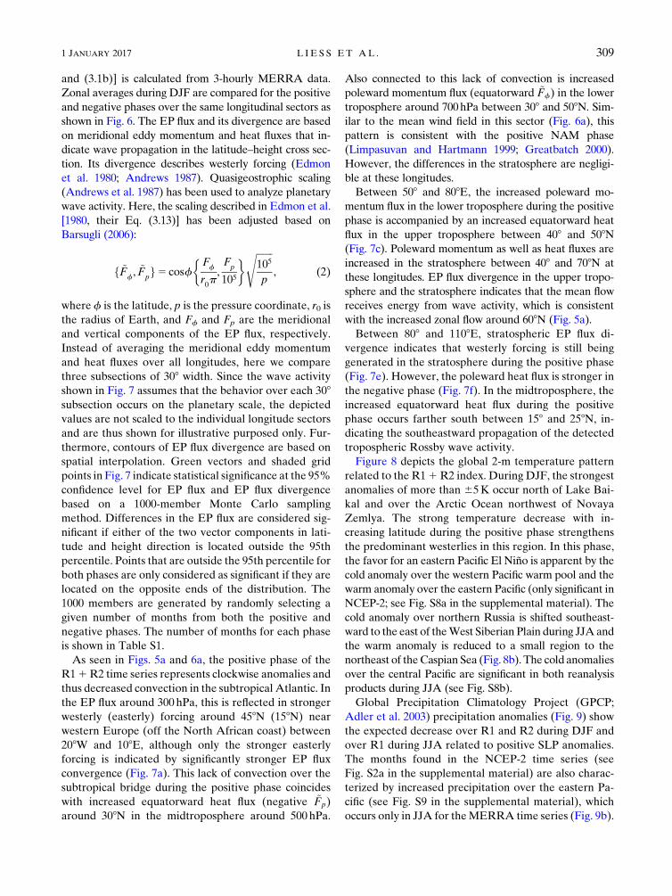
and (3.1b)] is calculated from 3-hourly MERRA data.Zonal averages during DJF are compared for the positiveand negative phases over the same longitudinal sectors asshown in Fig. 6. The EP flux and its divergence are basedon meridional eddy momentum and heat fluxes that in-dicate wave propagation in the latitude–height cross sec-tion. Its divergence describes westerly forcing (Edmonet al. 1980; Andrews 1987). Quasigeostrophic scaling(Andrews et al. 1987) has been used to analyze planetarywave activity. Here, the scaling described in Edmon et al.[1980, their Eq. (3.13)] has been adjusted based onBarsugli (2006):

f ~Ff, ~F

pg5 cosf

"Ff

r0p,Fp

105

# ffiffiffiffiffiffiffi105

p

s

, (2)

where f is the latitude, p is the pressure coordinate, r0 isthe radius of Earth, and Ff and Fp are the meridionaland vertical components of the EP flux, respectively.Instead of averaging the meridional eddy momentumand heat fluxes over all longitudes, here we comparethree subsections of 308 width. Since the wave activityshown in Fig. 7 assumes that the behavior over each 308subsection occurs on the planetary scale, the depictedvalues are not scaled to the individual longitude sectorsand are thus shown for illustrative purposed only. Fur-thermore, contours of EP flux divergence are based onspatial interpolation. Green vectors and shaded gridpoints in Fig. 7 indicate statistical significance at the 95%confidence level for EP flux and EP flux divergencebased on a 1000-member Monte Carlo samplingmethod. Differences in the EP flux are considered sig-nificant if either of the two vector components in lati-tude and height direction is located outside the 95thpercentile. Points that are outside the 95th percentile forboth phases are only considered as significant if they arelocated on the opposite ends of the distribution. The1000 members are generated by randomly selecting agiven number of months from both the positive andnegative phases. The number of months for each phaseis shown in Table S1.As seen in Figs. 5a and 6a, the positive phase of the

R11R2 time series represents clockwise anomalies andthus decreased convection in the subtropical Atlantic. Inthe EP flux around 300 hPa, this is reflected in strongerwesterly (easterly) forcing around 458N (158N) nearwestern Europe (off the North African coast) between208W and 108E, although only the stronger easterlyforcing is indicated by significantly stronger EP fluxconvergence (Fig. 7a). This lack of convection over thesubtropical bridge during the positive phase coincideswith increased equatorward heat flux (negative ~Fp)around 308N in the midtroposphere around 500 hPa.

Also connected to this lack of convection is increasedpoleward momentum flux (equatorward ~Ff) in the lowertroposphere around 700hPa between 308 and 508N. Sim-ilar to the mean wind field in this sector (Fig. 6a), thispattern is consistent with the positive NAM phase(Limpasuvan and Hartmann 1999; Greatbatch 2000).However, the differences in the stratosphere are negligi-ble at these longitudes.Between 508 and 808E, the increased poleward mo-

mentum flux in the lower troposphere during the positivephase is accompanied by an increased equatorward heatflux in the upper troposphere between 408 and 508N(Fig. 7c). Poleward momentum as well as heat fluxes areincreased in the stratosphere between 408 and 708N atthese longitudes. EP flux divergence in the upper tropo-sphere and the stratosphere indicates that the mean flowreceives energy from wave activity, which is consistentwith the increased zonal flow around 608N (Fig. 5a).Between 808 and 1108E, stratospheric EP flux di-

vergence indicates that westerly forcing is still beinggenerated in the stratosphere during the positive phase(Fig. 7e). However, the poleward heat flux is stronger inthe negative phase (Fig. 7f). In the midtroposphere, theincreased equatorward heat flux during the positivephase occurs farther south between 158 and 258N, in-dicating the southeastward propagation of the detectedtropospheric Rossby wave activity.Figure 8 depicts the global 2-m temperature pattern

related to the R11R2 index. During DJF, the strongestanomalies of more than 65K occur north of Lake Bai-kal and over the Arctic Ocean northwest of NovayaZemlya. The strong temperature decrease with in-creasing latitude during the positive phase strengthensthe predominant westerlies in this region. In this phase,the favor for an eastern Pacific El Niño is apparent by thecold anomaly over the western Pacific warm pool and thewarm anomaly over the eastern Pacific (only significant inNCEP-2; see Fig. S8a in the supplemental material). Thecold anomaly over northern Russia is shifted southeast-ward to the east of theWest Siberian Plain during JJA andthe warm anomaly is reduced to a small region to thenortheast of theCaspian Sea (Fig. 8b). The cold anomaliesover the central Pacific are significant in both reanalysisproducts during JJA (see Fig. S8b).Global Precipitation Climatology Project (GPCP;

Adler et al. 2003) precipitation anomalies (Fig. 9) showthe expected decrease over R1 and R2 during DJF andover R1 during JJA related to positive SLP anomalies.The months found in the NCEP-2 time series (seeFig. S2a in the supplemental material) are also charac-terized by increased precipitation over the eastern Pa-cific (see Fig. S9 in the supplemental material), whichoccurs only in JJA for theMERRA time series (Fig. 9b).

1 JANUARY 2017 L I E S S ET AL . 309

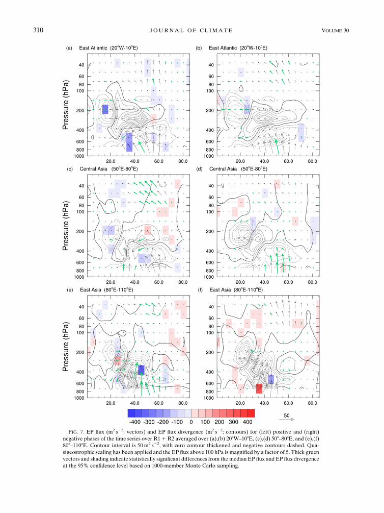
FIG. 7. EP flux (m2 s22; vectors) and EP flux divergence (m2 s22; contours) for (left) positive and (right)negative phases of the time series over R11 R2 averaged over (a),(b) 208W–108E, (c),(d) 508–808E, and (e),(f)808–1108E. Contour interval is 50 m2 s22, with zero contour thickened and negative contours dashed. Qua-sigeostrophic scaling has been applied and the EP flux above 100 hPa is magnified by a factor of 5. Thick greenvectors and shading indicate statistically significant differences from the median EP flux and EP flux divergenceat the 95% confidence level based on 1000-member Monte Carlo sampling.

310 JOURNAL OF CL IMATE VOLUME 30

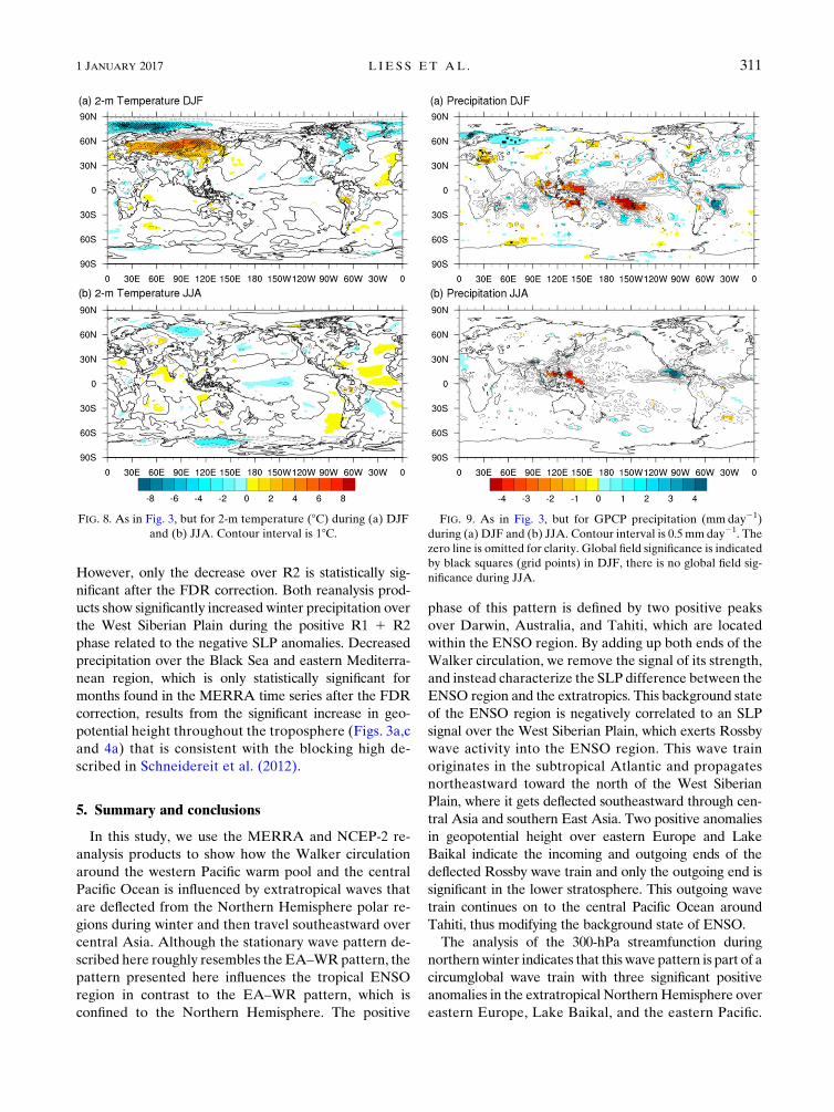
However, only the decrease over R2 is statistically sig-nificant after the FDR correction. Both reanalysis prod-ucts show significantly increased winter precipitation overthe West Siberian Plain during the positive R1 1 R2phase related to the negative SLP anomalies. Decreasedprecipitation over the Black Sea and eastern Mediterra-nean region, which is only statistically significant formonths found in the MERRA time series after the FDRcorrection, results from the significant increase in geo-potential height throughout the troposphere (Figs. 3a,cand 4a) that is consistent with the blocking high de-scribed in Schneidereit et al. (2012).

5. Summary and conclusions

In this study, we use the MERRA and NCEP-2 re-analysis products to show how the Walker circulationaround the western Pacific warm pool and the centralPacific Ocean is influenced by extratropical waves thatare deflected from the Northern Hemisphere polar re-gions during winter and then travel southeastward overcentral Asia. Although the stationary wave pattern de-scribed here roughly resembles the EA–WRpattern, thepattern presented here influences the tropical ENSOregion in contrast to the EA–WR pattern, which isconfined to the Northern Hemisphere. The positive

phase of this pattern is defined by two positive peaksover Darwin, Australia, and Tahiti, which are locatedwithin the ENSO region. By adding up both ends of theWalker circulation, we remove the signal of its strength,and instead characterize the SLP difference between theENSO region and the extratropics. This background stateof the ENSO region is negatively correlated to an SLPsignal over the West Siberian Plain, which exerts Rossbywave activity into the ENSO region. This wave trainoriginates in the subtropical Atlantic and propagatesnortheastward toward the north of the West SiberianPlain, where it gets deflected southeastward through cen-tral Asia and southern East Asia. Two positive anomaliesin geopotential height over eastern Europe and LakeBaikal indicate the incoming and outgoing ends of thedeflected Rossby wave train and only the outgoing end issignificant in the lower stratosphere. This outgoing wavetrain continues on to the central Pacific Ocean aroundTahiti, thus modifying the background state of ENSO.The analysis of the 300-hPa streamfunction during

northernwinter indicates that this wave pattern is part of acircumglobal wave train with three significant positiveanomalies in the extratropical NorthernHemisphere overeastern Europe, Lake Baikal, and the eastern Pacific.

FIG. 9. As in Fig. 3, but for GPCP precipitation (mmday21)during (a) DJF and (b) JJA. Contour interval is 0.5mmday21. Thezero line is omitted for clarity. Global field significance is indicatedby black squares (grid points) in DJF, there is no global field sig-nificance during JJA.

FIG. 8. As in Fig. 3, but for 2-m temperature (8C) during (a) DJFand (b) JJA. Contour interval is 18C.

1 JANUARY 2017 L I E S S ET AL . 311

A fourth positive anomaly over the tropical Pacific andsubtropical Atlantic reveals the subtropical bridge(Tang and Neelin 2004; Graf and Zanchettin 2012;Park and Dusek 2013). Negative anomalies exist to thenorth over Novaya Zemlya, the northeastern Pacific,and the Labrador Sea. Over Eurasia, this patternindicates a strengthened polar jet stream around 608Nand a weakened East Asian jet stream (EAJS) around408N. The positive phase of the above described wavetrain can also be associated with positive phases of thePNA and NAO patterns. Most prominently however,the association of this circumglobal wave train withthe ENSO region indicates that the wave train from theWest Siberian Plain is related to opposite phases of theeastern Pacific and central Pacific El Niño events.A similar but less significant signal can be detected

during northern spring and fall (not shown here). Duringsummer, however, the signal of the correlation is re-versed and not significant. Only a composite analysis ofJJA reanalysis data shows significant patterns of a sta-tionary wave over central and East Asia. The seasonalchanges in the detected signal make it difficult to use thissignal as a predictive tool and more interpretation isnecessary to fully understand the implications of theteleconnections described here.In general, the AMO influence on Rossby wave activity

in the subtropical North Atlantic suggests a multidecadalcomponent in the detectedwave train.Hu andFeng (2012)investigated the combined impact of ENSO and AMO onsummertime precipitation in North America. The AMOcauses an asymmetry in precipitation response to El Niñoand La Niña, whereby summertime precipitation has amuch larger positive anomaly in El Niño years occurringduring the warm phase of the AMO than during the coldphase of the AMO. Although the impact of the detectedwave train on regional precipitation is largely confined tothe regions R1, R2, andR3, as well as to the Black Sea andeasternMediterranean region in our analysis, temperatureanomalies can be as large as 65K north of Lake Baikaland over the Arctic Ocean northwest of Novaya Zemlya.In conclusion, it should be noted that the atmosphericimpact on the ENSO region should be taken into accountfor the characterization of global ENSO signals.

Acknowledgments. The authors thank three anony-mous reviewers for detailed criticisms that led to animproved paper. MERRA reanalysis data were pro-vided by NASA’s Modeling and Assimilation Data andInformation Services Center, the NCEP-2 reanalysisand GPCP data were received from NOAA’s EarthSystem Research Laboratory, and HadSLP2 data wereobtained from the Met Office (UKMO). This study wassupported by theU.S. National Science Foundation under

Grant 1029711, the National Aeronautics and Space Ad-ministration underGrantNNX16AB21G, and theGeorgeR. and Orpha Gibson Foundation at the University ofMinnesota. Computing facilities were made available bythe Minnesota Supercomputing Institute.

APPENDIX

Combining Correlations

For three normalized time series T1, T2, and T3, eachobserved over T time stamps, the covariance obeys theidentity

cov(T11T

2,T

3)5 cov(T

1,T

3)1 cov(T

2,T

3) (A1)

(Snedecor and Cochran 1989).This identity can be used for correlations so that

corr(T1 1T2,T3)

5cov(T

1,T

3)1 cov(T

2,T

3)

ffiffiffiffiffiffiffiffiffiffiffiffiffiffiffiffiffiffiffiffiffiffiffiffiffiffiffiffiffiffiffiffiffiffiffiffiffiffiffiffiffiffiffiffiffiffiffiffiffiffiffiffiffiffiffiffiffiffiffiffiffiffiffiffiffiffiffiffivar(T

1)1 var(T

2)1 2cov(T

1,T

2)

p ffiffiffiffiffiffiffiffiffiffiffiffiffiffiffiffivar(T

3)

p :

(A2)

Since all time series are normalized, var(Ti) 5 1, andthus

corr(T1 1T2,T3)

5corr(T

1,T

3)1 corr(T

2,T

3)

ffiffiffiffiffiffiffiffiffiffiffiffiffiffiffiffiffiffiffiffiffiffiffiffiffiffiffiffiffiffiffiffiffiffiffiffiffiffiffiffiffiffiffi11 11 2corr(T

1,T

2)

p ffiffiffi1

p or

5corr(T

1,T

3)1 corr(T

2,T

3)

ffiffiffiffiffiffiffiffiffiffiffiffiffiffiffiffiffiffiffiffiffiffiffiffiffiffiffiffiffiffiffiffiffiffiffiffiffiffi2[11 corr(T

1,T

2)]

p . (A3)

REFERENCES

Adler, R. F., and Coauthors, 2003: The version-2 Global Pre-cipitation Climatology Project (GPCP) monthly precipitationanalysis (1979–present). J. Hydrometeor., 4, 1147–1167,doi:10.1175/1525-7541(2003)004,1147:TVGPCP.2.0.CO;2.

Agrawal, S., G. Atluri, S. Liess, S. Chatterjee, and V. Kumar, 2015:Tripoles: A new class of climate teleconnections. University ofMinnesotaDepartment of Computer Science andEngineeringTech. Rep. TR 15-020, 22 pp. [Available online at https://www.cs.umn.edu/sites/cs.umn.edu/files/tech_reports/15-020.pdf.]

Allan, R., and T. Ansell, 2006: A new globally complete monthlyhistorical griddedmean sea level pressure dataset (HadSLP2):1850–2004. J. Climate, 19, 5816–5842, doi:10.1175/JCLI3937.1.

Andrews, D. G., 1987: On the interpretation of the Eliassen-Palmflux divergence. Quart. J. Roy. Meteor. Soc., 113, 323–338,doi:10.1002/qj.49711347518.

——, F. W. Taylor, and M. E. McIntyre, 1987: The influence ofatmospheric waves on the general circulation of the middleatmosphere. Philos. Trans. Roy. Soc. London, 323A, 693–705,doi:10.1098/rsta.1987.0115.

312 JOURNAL OF CL IMATE VOLUME 30

Baldwin, M. P., and T. J. Dunkerton, 2001: Stratospheric harbin-gers of anomalous weather regimes. Science, 294, 581–584,doi:10.1126/science.1063315.

Barnston, A. G., and R. E. Livezey, 1987: Classification, sea-sonality and persistence of low-frequency atmospheric cir-culation patterns.Mon.Wea. Rev., 115, 1083–1126, doi:10.1175/1520-0493(1987)115,1083:CSAPOL.2.0.CO;2.

Barsugli, J., 2006: EP fluxes. NOAA/ESRL Physical Sciences Di-vision. [Available online at http://www.esrl.noaa.gov/psd/data/epflux/.]

Benjamini, Y., and Y. Hochberg, 1995: Controlling the false dis-covery rate: A practical and powerful approach to multipletesting. J. Roy. Stat. Soc., 57B, 289–300. [Available online athttp://www.jstor.org/stable/2346101.]

——, andD. Yekutieli, 2001: The control of the false discovery ratein multiple testing under dependency. Ann. Stat., 29, 1165–1188, doi:10.1214/aos/1013699998.

Brönnimann, S., E. Xoplaki, C. Casty, A. Pauling, andJ. Luterbacher, 2007: ENSO influence on Europe during thelast centuries. Climate Dyn., 28, 181–197, doi:10.1007/s00382-006-0175-z.

Chhak, K. C., E. Di Lorenzo, N. Schneider, and P. F. Cummins,2009: Forcing of low-frequency ocean variability in thenortheast Pacific. J. Climate, 22, 1255–1276, doi:10.1175/2008JCLI2639.1.

Cohen, J., M. Barlow, and K. Saito, 2009: Decadal fluctuations inplanetary wave forcing modulate global warming in late borealwinter. J. Climate, 22, 4418–4426, doi:10.1175/2009JCLI2931.1.

——, J. C. Furtado, J. Jones, M. Barlow, D. Whittleston, andD.Entekhabi, 2014: Linking Siberian snowcover to precursors ofstratospheric variability. J. Climate, 27, 5422–5432, doi:10.1175/JCLI-D-13-00779.1.

Deser, C., A. S. Phillips, and J. W. Hurrell, 2004: Pacific interdecadalclimate variability: Linkages between the tropics and the NorthPacific during boreal winter since 1900. J.Climate, 17, 3109–3124,doi:10.1175/1520-0442(2004)017,3109:PICVLB.2.0.CO;2.

——,M. A. Alexander, S.-P. Xie, and A. S. Phillips, 2010: Sea surfacetemperature variability: Patterns and mechanisms. Annu. Rev.Mar. Sci., 2, 115–143, doi:10.1146/annurev-marine-120408-151453.

Dettinger,M.D.,D.R.Cayan,G. J.McCabe, and J.A.Marengo, 2000:Multiscale streamflowvariability associatedwithElNiño/SouthernOscillation. El Niño and the Southern Oscillation: MultiscaleVariability and Global and Regional Impacts, H. F. Diaz andV. Markgraf, Eds., Cambridge University Press, 113–146.

Di Lorenzo, E., K. M. Cobb, J. C. Furtado, N. Schneider, B. T.Anderson,A. Bracco,M.A.Alexander, andD. J. Vimont, 2010:Central Pacific El Niño and decadal climate change in theNorthPacific Ocean. Nat. Geosci., 3, 762–765, doi:10.1038/ngeo984.

Dima, M., and G. Lohmann, 2007: A hemispheric mechanism forthe Atlantic multidecadal oscillation. J. Climate, 20, 2706–2719, doi:10.1175/JCLI4174.1.

Ding, Q., and B. Wang, 2005: Circumglobal teleconnection in theNorthern Hemisphere summer. J. Climate, 18, 3483–3505,doi:10.1175/JCLI3473.1.

Domeisen, D. I. V., L. Sun, andG. Chen, 2013: The role of synopticeddies in the tropospheric response to stratospheric variabil-ity. Geophys. Res. Lett., 40, 4933–4937, doi:10.1002/grl.50943.

Dommenget, D., and M. Latif, 2002: A cautionary note on the in-terpretation of EOFs. J. Climate, 15, 216–225, doi:10.1175/1520-0442(2002)015,0216:ACNOTI.2.0.CO;2.

Edmon,H. J., B. J.Hoskins, andM.E.McIntyre, 1980:Eliassen–Palmcross sections for the troposphere. J. Atmos. Sci., 37, 2600–2616,doi:10.1175/1520-0469(1980)037,2600:EPCSFT.2.0.CO;2.

Fang, K., F. Chen, A. K. Sen, N. Davi, W. Huang, J. Li, andH. Seppä, 2014: Hydroclimate variations in central and mon-soonal Asia over the past 700 years. PLoS One, 9, e102751,doi:10.1371/journal.pone.0102751.

Fedorov, A. V., S. Hu, M. Lengaigne, and E. Guilyardi, 2015: Theimpact of westerly wind bursts and ocean initial state on thedevelopment, and diversity of El Niño events. Climate Dyn.,44, 1381–1401, doi:10.1007/s00382-014-2126-4.

Feldstein, S. B., 2003: The dynamics of NAO teleconnection pat-tern growth and decay. Quart. J. Roy. Meteor. Soc., 129, 901–924, doi:10.1256/qj.02.76.

Foster, J. L., J. Cohen, D. A. Robinson, and T. W. Estilow, 2013:A look at the date of snowmelt and correlations with theArctic Oscillation. Ann. Glaciol., 54, 196–204, doi:10.3189/2013AoG62A090.

Franzke, C., S. B. Feldstein, and S. Lee, 2011: Synoptic analysis ofthe Pacific–North American teleconnection pattern. Quart.J. Roy. Meteor. Soc., 137, 329–346, doi:10.1002/qj.768.

Garfinkel, C. I., and D. L. Hartmann, 2008: Different ENSO tele-connections and their effects on the stratospheric polar vortex.J. Geophys. Res., 113, D18114, doi:10.1029/2008JD009920.

Gershunov, A., and T. P. Barnett, 1998: Interdecadal modulation ofENSO teleconnections.Bull. Amer.Meteor. Soc., 79, 2715–2725,doi:10.1175/1520-0477(1998)079,2715:IMOET.2.0.CO;2.

Gillett, N. P., and P. A. Stott, 2009: Attribution of anthropogenicinfluence on seasonal sea level pressure. Geophys. Res. Lett.,36, L23709, doi:10.1029/2009GL041269.

Gollan, G., R. J. Greatbatch, and T. Jung, 2012: Tropical impact onthe East Asian winter monsoon. Geophys. Res. Lett., 39,L17801, doi:10.1029/2012GL052978.

Gonsamo, A., J. M. Chen, and P. D’Odorico, 2015: Under-estimated role of east Atlantic–west Russia pattern on Ama-zon vegetation productivity. Proc. Natl. Acad. Sci. USA, 112,E1054–E1055, doi:10.1073/pnas.1420834112.

Gouirand, I., and V. Moron, 2003: Variability of the impact of ElNiño–Southern Oscillation on sea-level pressure anomaliesover the North Atlantic in January to March (1874–1996). Int.J. Climatol., 23, 1549–1566, doi:10.1002/joc.963.

Graf, H.-F., and D. Zanchettin, 2012: Central Pacific El Niño, the‘‘subtropical bridge,’’ and Eurasian climate. J. Geophys. Res.,117, D01102, doi:10.1029/2011JD016493.

Greatbatch, R. J., 2000: The North Atlantic Oscillation. StochasticEnviron. Res. Risk Assess., 14, 213–242, doi:10.1007/s004770000047.

Hu, Q., and S. Feng, 2012: AMO- and ENSO-driven summertimecirculation and precipitation variations in North America.J. Climate, 25, 6477–6495, doi:10.1175/JCLI-D-11-00520.1.

Jia, L.-H., H.-Y. Li, R.-Q. Li, H. Tang, and W. Huo, 2012: Nu-merical simulation and diagnosis analysis of ‘‘3.12’’ sandstormin south Xinjiang. J. Desert Res., 32, 1135–1141. [Availableonline at http://zgsm.westgis.ac.cn/EN/abstract/abstract2258.shtml.]

Kanamitsu, M., W. Ebisuzaki, J. Woollen, S.-K. Yang, J. J. Hnilo,M. Fiorino, and G. L. Potter, 2002: NCEP–DOE AMIP-IIreanalysis (R-2). Bull. Amer. Meteor. Soc., 83, 1631–1643,doi:10.1175/BAMS-83-11-1631.

Kawale, J., M. Steinbach, and V. Kumar, 2011: Discovering dynamicdipoles in climate data. Proc. 2011 SIAM Int. Conf. on DataMining, Philadelphia, PA, Society for Industrial and AppliedMathematics, 107–118, doi:10.1137/1.9781611972818.10.

——, and Coauthors, 2013: A graph-based approach to find tele-connections in climate data. Stat. Anal. Data Min., 6, 158–179,doi:10.1002/sam.11181.

1 JANUARY 2017 L I E S S ET AL . 313

Kayano, M. T., and V. B. Capistrano, 2014: How the Atlanticmultidecadal oscillation (AMO)modifies the ENSO influenceon the South American rainfall. Int. J. Climatol., 34, 162–178,doi:10.1002/joc.3674.

Kim, H.-M., P. J. Webster, and J. A. Curry, 2009: Impact ofshifting patterns of Pacific Ocean warming on North At-lantic tropical cyclones. Science, 325, 77–80, doi:10.1126/science.1174062.

Krichak, S. O., and P. Alpert, 2005: Decadal trends in the eastAtlantic–west Russia pattern and Mediterranean pre-cipitation. Int. J. Climatol., 25, 183–192, doi:10.1002/joc.1124.

Kug, J.-S., F.-F. Jin, and S.-I. An, 2009: Two types of El Niñoevents: Cold tongue El Niño and warm pool El Niño.J. Climate, 22, 1499–1515, doi:10.1175/2008JCLI2624.1.

Kumar, A., H. Wang, W. Wang, Y. Xue, and Z.-Z. Hu, 2013: Doesknowing the oceanic PDO phase help predict the atmosphericanomalies in subsequent months? J. Climate, 26, 1268–1285,doi:10.1175/JCLI-D-12-00057.1.

Kunz, T., and R. J. Greatbatch, 2013: On the northern annularmode surface signal associated with stratospheric variability.J. Atmos. Sci., 70, 2103–2118, doi:10.1175/JAS-D-12-0158.1.

Larkin, N. K., and D. E. Harrison, 2005: On the definition ofEl Niño and associated seasonal average U.S. weatheranomalies. Geophys. Res. Lett., 32, L13705, doi:10.1029/2005GL022738.

Li, Y.-P., G. Dele, Q. Si, and X.-H. Wu, 2013: A synoptic analysison forecasting of sand-dust storm in November over InnerMongolia. J. Desert Res., 33, 1483–1491. [Available online athttp://zgsm.westgis.ac.cn/EN/abstract/abstract2550.shtml.]

Liao, Q.-H., S.-Y. Tao, andH.-J.Wang, 2004: Interannual variationof summer subtropical westerly jet in East Asia and its impactson the climate anomalies of EastAsia summermonsoon.Chin.J. Geophys., 47, 12–21, doi:10.1002/cjg2.449.

Liess, S., and Coauthors, 2014: Different modes of variability overthe Tasman Sea: Implications for regional climate. J. Climate,27, 8466–8486, doi:10.1175/JCLI-D-13-00713.1.

Limpasuvan,V., andD. L.Hartmann, 1999: Eddies and the annularmodes of climate variability. Geophys. Res. Lett., 26, 3133–3136, doi:10.1029/1999GL010478.

Marullo, S., V. Artale, and R. Santoleri, 2011: The SST multi-decadal variability in the Atlantic–Mediterranean region andits relation to AMO. J. Climate, 24, 4385–4401, doi:10.1175/2011JCLI3884.1.

Newman, M., and P. D. Sardeshmukh, 1995: A caveat concerningsingular value decomposition. J. Climate, 8, 352–360, doi:10.1175/1520-0442(1995)008,0352:ACCSVD.2.0.CO;2.

Nowlin, W. D., Jr., and J. M. Klinck, 1986: The physics of theAntarctic Circumpolar Current. Rev. Geophys., 24, 469–491,doi:10.1029/RG024i003p00469.

Park, J., and G. Dusek, 2013: ENSO components of the Atlanticmultidecadal oscillation and their relation to North Atlanticinterannual coastal sea level anomalies. Ocean Sci., 9, 535–543, doi:10.5194/os-9-535-2013.

Philander, S. G. H., and R. C. Pacanowski, 1981: Response ofequatorial oceans to periodic forcing. J. Geophys. Res., 86,1903–1916, doi:10.1029/JC086iC03p01903.

Power, S., T. Casey, C. Folland, A. Colman, and V. Mehta,1999: Inter-decadal modulation of the impact of ENSO onAustralia. Climate Dyn., 15, 319–324, doi:10.1007/s003820050284.

Ren, X., X. Yang, and C. Chu, 2010: Seasonal variations of thesynoptic-scale transient eddy activity andpolar front jet overEastAsia. J. Climate, 23, 3222–3233, doi:10.1175/2009JCLI3225.1.

Rienecker, M. M., and Coauthors, 2011: MERRA: NASA’sModern-Era Retrospective Analysis for Research andApplications. J. Climate, 24, 3624–3648, doi:10.1175/JCLI-D-11-00015.1.

Ropelewski, C. F., and M. S. Halpert, 1986: North Americanprecipitation and temperature patterns associated with theEl Niño/Southern Oscillation (ENSO). Mon. Wea. Rev.,114, 2352–2362, doi:10.1175/1520-0493(1986)114,2352:NAPATP.2.0.CO;2.

Schneidereit, A., S. Schubert, P. Vargin, F. Lunkeit, X. Zhu,D. H. W. Peters, and K. Fraedrich, 2012: Large-scale flowand the long-lasting blocking high over Russia: Summer2010. Mon. Wea. Rev., 140, 2967–2981, doi:10.1175/MWR-D-11-00249.1.

Semazzi, F., and Coauthors, 2015: Decadal variability of the EastAfrican monsoon. CLIVAR Exchanges, No. 66, InternationalCLIVARProjectOffice, Southampton,UnitedKingdom, 15–19.[Available online at http://www.clivar.org/sites/default/files/documents/CLIVAR_Exchanges_No_66_Final_with_bleed_23_June_15.pdf.]

Simmonds, I., 2015: Comparing and contrasting the behaviour ofArctic and Antarctic sea ice over the 35 year period 1979–2013. Ann. Glaciol., 56, 18–28, doi:10.3189/2015AoG69A909.

Smoliak, B. V., and J. M. Wallace, 2015: On the leading patterns ofNorthern Hemisphere sea level pressure variability. J. Atmos.Sci., 72, 3469–3486, doi:10.1175/JAS-D-14-0371.1.

Snedecor, G.W., andW. G. Cochran, 1989: Statistical Methods. 8thed. Iowa State University Press, 503 pp.

Tang, B. H., and J. D. Neelin, 2004: ENSO influence on Atlantichurricanes via tropospheric warming. Geophys. Res. Lett., 31,L24204, doi:10.1029/2004GL021072.

Teegavarapu, R. S. V., A. Goly, and J. Obeysekera, 2013: In-fluences of Atlantic multidecadal oscillation phases on spatialand temporal variability of regional precipitation extremes.J. Hydrol., 495, 74–93, doi:10.1016/j.jhydrol.2013.05.003.

Trenberth, K. E., 1981: Seasonal variations in global sea levelpressure and the total mass of the atmosphere. J. Geophys.Res., 86, 5238–5246, doi:10.1029/JC086iC06p05238.

——, and C. J. Guillemot, 1996: Physical processes involved inthe 1988 drought and 1993 floods in North America.J. Climate, 9, 1288–1298, doi:10.1175/1520-0442(1996)009,1288:PPIITD.2.0.CO;2.

Verdon, D. C., and S. W. Franks, 2006: Long-term behaviour ofENSO: Interactions with the PDO over the past 400 yearsinferred from paleoclimate records. Geophys. Res. Lett., 33,L06712, doi:10.1029/2005GL025052.

Wallace, J. M., and D. S. Gutzler, 1981: Teleconnections inthe geopotential height field during the Northern Hemi-sphere winter. Mon. Wea. Rev., 109, 784–812, doi:10.1175/1520-0493(1981)109,0784:TITGHF.2.0.CO;2.

Wang, B., R. Wu, and X. Fu, 2000: Pacific–East Asian teleconnec-tion: How does ENSO affect East Asian climate? J. Climate,13, 1517–1536, doi:10.1175/1520-0442(2000)013,1517:PEATHD.2.0.CO;2.

Wang, L., W. Chen, and R. Huang, 2008: Interdecadal modulationof PDO on the impact of ENSO on the East Asian wintermonsoon. Geophys. Res. Lett., 35, L20702, doi:10.1029/2008GL035287.

Wilks, D. S., 2006: On ‘‘field significance’’ and the false discoveryrate. J. Appl. Meteor. Climatol., 45, 1181–1189, doi:10.1175/JAM2404.1.

——, 2016: ‘‘The stippling shows statistically significant grid-points’’: How research results are routinely overstated and

314 JOURNAL OF CL IMATE VOLUME 30

overinterpreted, and what to do about it. Bull. Amer. Meteor.Soc., doi:10.1175/BAMS-D-15-00267.1, in press.

Xie, R., F. Huang, F.-F. Jin, and J. Huang, 2015: The impact of basicstate on quasi-biennial periodicity of central Pacific ENSO overthe past decade. Theor. Appl. Climatol., 120, 55–67, doi:10.1007/s00704-014-1150-y.

Yang, S., K.-M. Lau, and K.-M. Kim, 2002: Variations of theEast Asian jet stream and Asian–Pacific–American winterclimate anomalies. J. Climate, 15, 306–325, doi:10.1175/1520-0442(2002)015,0306:VOTEAJ.2.0.CO;2.

Yu, J.-Y., and S. T. Kim, 2013: Identifying the types of major El Niñoevents since 1870. Int. J. Climatol., 33, 2105–2112, doi:10.1002/joc.3575.

Zanchettin, D., O. Bothe, W. Müller, J. Bader, and J. H.Jungclaus, 2014: Different flavors of the Atlantic multi-decadal variability. Climate Dyn., 42, 381–399, doi:10.1007/s00382-013-1669-0.

Zhang, Y., J. M. Wallace, and D. S. Battisti, 1997: ENSO-like in-terdecadal variability: 1900–93. J. Climate, 10, 1004–1020,doi:10.1175/1520-0442(1997)010,1004:ELIV.2.0.CO;2.

1 JANUARY 2017 L I E S S ET AL . 315